Article

Experimental Study and Modeling of Ground-SourceHeat Pumps with Combi-Storage in Buildings

Wessam El-Baz* 1 ID , Peter Tzscheutschler 1 ID and Ulrich Wagner 1

1 Institute of Energy Economy and Application Technology, Technical University of Munich. Arcisstr. 21 80333Munich, Germany

* Correspondence: wessam.elbaz@tum.de; Tel.: +49-(0)89-289-28314

Abstract: There is a continuous growth of heat pump installations in residential buildings in Germany.The heat pumps are not only used for space heating and domestic hot water consumption but alsoto offer flexibility to the grid. The high coefficient of performance and the low cost of heat storagesmade the heat pumps one of the optimal candidates for the power to heat applications. Thus, severalquestions are raised about the optimal integration and control of the heat pump system with bufferstorages to maximize its operation efficiency and minimize the operation costs. In this paper, anexperimental investigation is performed to study the performance of a ground source heat pump(GSHP) with a combi-storage under several configurations and control factors. The experiments wereperformed on an innovative modular testbed that is capable of emulating a ground source to providethe heat pump with different temperature levels at different times of the day. Moreover, it can emulatethe different building loads such as the space heating load and the domestic hot water consumptionin real-time. The data gathered from the testbed and different experimental studies were used todevelop a simulation model based on Modelica that can accurately simulate the dynamics of a GSHPin a building. The model was validated based on different metrics. Energetically, the differencebetween the developed model and the measured values was only 3% and 4% for the heat generationand electricity consumption, respectively.

Keywords: Modelica; testbed; control requirements; modeling; EMS; sensor placement;

0. Introduction

In the German power sector, an ongoing increase of renewable energy integration can be witnessed.In 2016, 29% of gross generated electricity was produced from renewable energy sources’ (RES’s),which represents 192 TWh [1]. Such increase in the RES’s integration is empowered by several policiessuch as the renewable energy act (EEG) [2]. The act guarantees the generator a fixed price overa specific term, which gives a priority to the RES in the electricity market. Having such weatherdependent fluctuating RES in the market, raised the demand for flexibility to balance the fluctuatinggeneration. Sector coupling presented one way to mitigate the fluctuating RES and offer flexibilityto the grid. Hence, it is receiving continuous attention not only within the research communities butalso on the political and industrial level. Coupling the power to the heat sector is seen as one of themost influential and attractive approaches to decarbonize the heat sector and gain additional flexibilityin power gird [3]. Considering that the consumed heat energy in Germany within different sectorswas 1,373 TWh in 2016 [4], there is a substantial room for power to heat application integration. Anadvantage of such applications is its attractive costs due to its dependency on heat storage that hassignificantly lower costs compared to batteries.

The heat pump is a major role player in sector coupling due to the progressive improvementof the coefficient of performance (COP) [5]. Hence, the number of heat pumps installations are on

Preprints (www.preprints.org) | NOT PEER-REVIEWED | Posted: 13 April 2018 doi:10.20944/preprints201804.0183.v1

© 2018 by the author(s). Distributed under a Creative Commons CC BY license.

Peer-reviewed version available at Energies 2018, 11, 1174; doi:10.3390/en11051174

2 of 18

continuous growth on yearly basis, especially in the residential sector. According to [6], the heat pumpinstallations in new buildings in 2016 reached 31.8%. Heat pump represents 34% of the market shareof the single-family houses, 16% of the multi-family houses and 13.6% of the non-residential buildings.Such widespread of the heat pump raised research questions focusing not only on the heat pumpcycle and components improvement but also on a better integration and control of the heat pump as asystem.

The topics discussed within the literature covered large scope such as the thermodynamic cycleand compressor optimizations [7–10] hydraulic system configurations [11], performance evaluation[12,13], and integration in district heating and smart grids [5,14]. The research presented can bedivided into experimental studies and numerical studies. The experimental studies were mostlyoriented towards cycle and components optimization of the heat pumps. In [15], a carbon dioxidedirect-expansion heat pump was investigated in different operating conditions. [16] studied theperformance of solar ground source heat pump in dual heat source coupling modes to optimizethe average system COP. Furthermore, [17] experimentally tested a gas engine driven heat pumpfor different operation modes. The author developed a prototype to test the heating and coolingperformance for different evaporator’s inlet temperatures, ambient temperatures, and gas enginespeeds. The numerical studies and simulations were utilized, where experimental studies wouldbe costly. In [18], a heat pump was simulated to cover the load of a multi-zone office building.While in [19], a simulation model was developed to analyze the flow pumping of ground source heatpumps. [20] developed a numerical model for a reversible multi-function heat pump to evaluate itsperformance in summer for domestic hot water (DHW) and space cooling. The numerical model wasthen evaluated against a model in TRNSYS.

In the residential sector, several studies were performed on air-source heat pumps (ASHP)and ground-source heat pumps (GSHP). The presented studies were mostly numerical. Also, it isoriented towards optimizing the heat pump control, system dimension and hydraulics to minimizethe operation costs and maximize the use of renewable energies within the residential building asin [21–25]. Although numerical studies can provide relatively proper indicator of the behavior of asystem, it is exposed to several uncertainties and its accuracy is always questioned, especially if thestudied object is a thermodynamic system. Studies analyzing large models on the district level ormicro grid levels have mostly 1-h resolution as in the review of [3], consequently, all dynamics of theheat pump systems are concealed. Moreover, in several cases, the COP is assumed to be constant andall the nonlinearities are ignored so that the optimization problem can converge faster. Yet, this exposesthe model to inevitable uncertainties. On the building level, dynamic systems simulation programs areused such as TRNSYS or Modelica-based software as Simulation X [26]. These programs can detail thedynamics of the systems, yet as discussed in [27], calibration is rather complicated. Moreover, thesemodels are mostly validated by a plausibility check, but not against measured values. Field tests wereperformed to investigate the performance of heat pumps [12]. These studies can provide a realisticinvestigation of the performance of heat pumps in general, yet it does not offer the flexibility of anexperimental system to vary different parameter and it can conceal several details that can contributeto the understanding of the system.

0.1. Objectives

To provide realistic reliable results, numerical studies have to be always supported byexperimental results. Otherwise, any presented control system, mathematical model, or simulationmodel might be exposed to imminent uncertainties. In this paper, an experimental study is performedto validate a numerical model and present the optimal control requirements for a GSHP in a residentialbuilding. The experimental study does not only include a residential commercial heat pump and acombi-buffer storage but also a building load emulator to integrate the real space heating (SH) andDHW load of the building. The objectives of this paper can be summarized in the following:

Preprints (www.preprints.org) | NOT PEER-REVIEWED | Posted: 13 April 2018 doi:10.20944/preprints201804.0183.v1

Peer-reviewed version available at Energies 2018, 11, 1174; doi:10.3390/en11051174

3 of 18

• Presenting a novel modular heat pump testbed design that emulates a complete residentialhouse. It includes a ground-source emulator, combi-buffer heat storage, and a building loademulator. The testbed is designed to be integrated with different heat pump types and hydraulicconnections, so that it can be used for standardization applications, control and optimizationmethods performance testing, and models validation• Based on multiple experimental testing, the real-life optimal control criteria for a commercial

residential GSHP under the given constraints of the heat pumps manufactures have beenidentified.• Demonstrating a modelica-based heat pump model that can be easily integrated into building

and district simulations due to its minimal computational requirements. The model was alsovalidated and calibrated based on the experimental data of the presented testbed.

The structure of this paper is as follows: Section 1 describes the design and components of the testbed.Moreover, it introduces the measurements system used and discusses the testbed control dynamics.Section 2 presents the experimental testing procedure and its purpose. Section 3 presents the validatedModelica heat pump model and its structure. Section 4 discusses the results of the experimental testingand the validation of the Modelica model. Section 5 presents a conclusive summary of the experimentalstudy and the model performance.

1. Experimental System Description

1.1. Overview

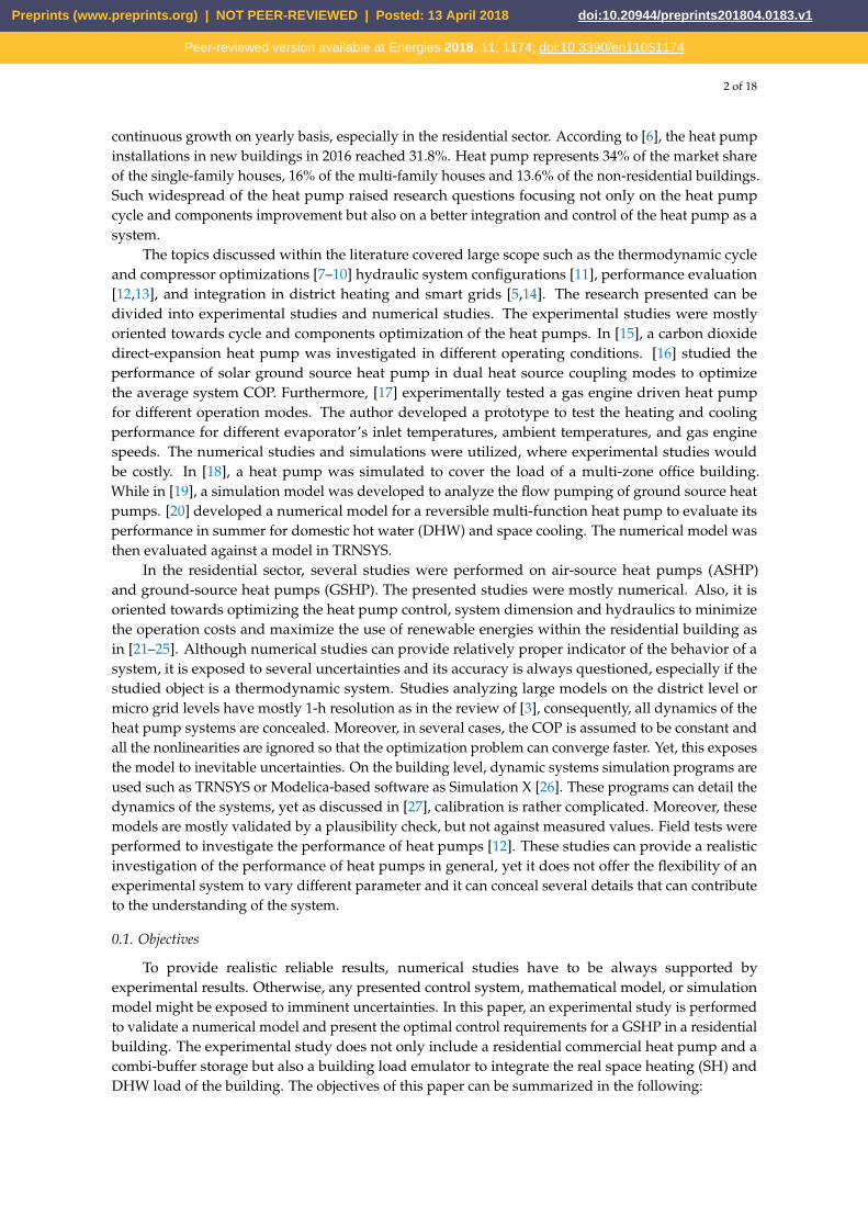
The testbed consists of 3 different modules: ground-source emulator (A), combi-storage (B), andthe building loads emulator (C). Figure 1 and 2 show a simplified hydraulic scheme and the realtestbed, respectively. The presented hydraulic configuration is not a permanent configuration, butrather the one used for the experiments documented in this paper. Other possible configuration can bealso implemented such as a direct connection between the heat pump and module C, replacing moduleB with a DHW tank module, or having two separate modules for a DHW tank and a buffer tank.Each module has its own independent control and measurement system to facilitate the integration ofdifferent modules. The GSHP used is a STIEBEL ELTRON WPF10 heat pump with a thermal powerof 10.31 kW and a COP of 5.02 by B0/W35 according to the standard EN 14511. A brine pump andheating system circulation pump is already integrated within the GSHP. Moreover, the GSHP is alsoequipped with an emergency/backup electrical heater of 8.8 kW.

Figure 1. Simplified hydraulic scheme of the testbed

Preprints (www.preprints.org) | NOT PEER-REVIEWED | Posted: 13 April 2018 doi:10.20944/preprints201804.0183.v1

Peer-reviewed version available at Energies 2018, 11, 1174; doi:10.3390/en11051174

4 of 18

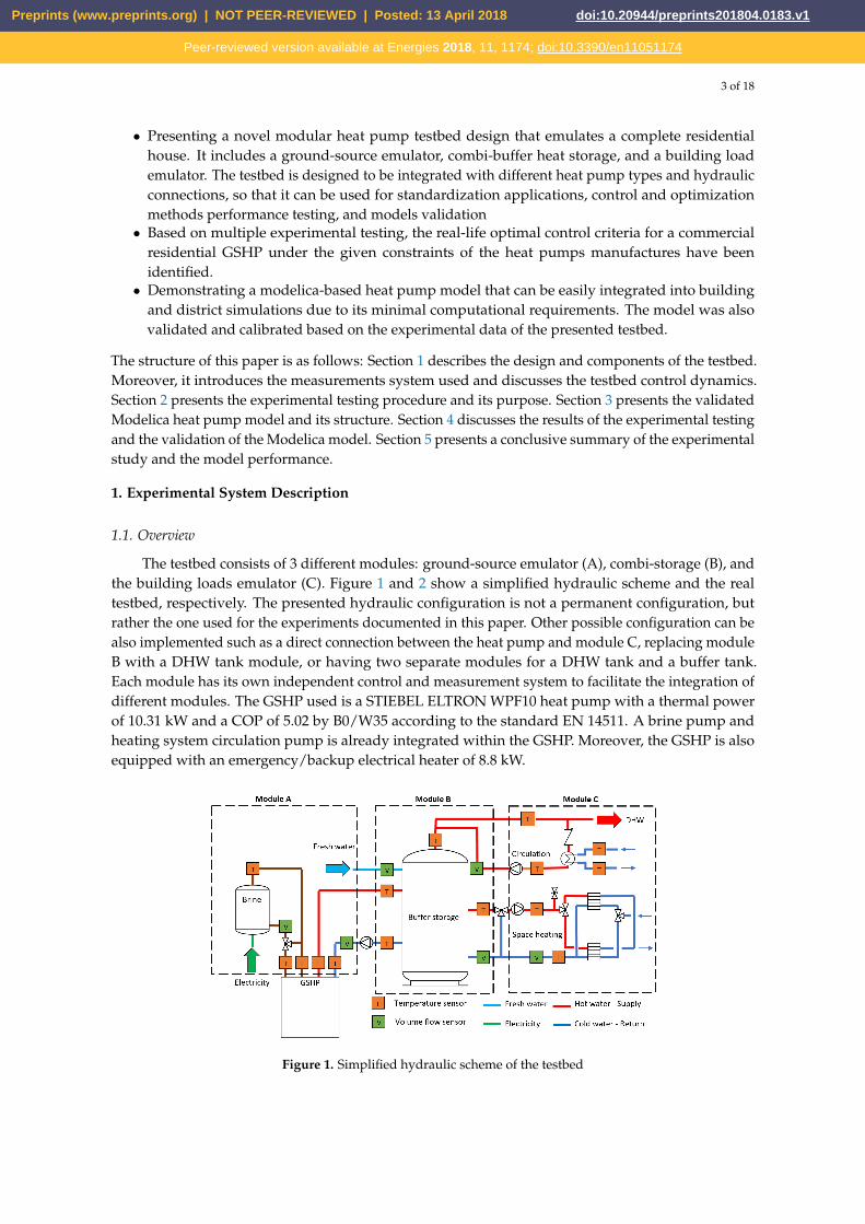
Figure 2. The 3 modules and the heat pump installation in the lab

1.2. Module A: ground-source emulator

Module A emulates a ground-source, which is equivalent to a controlled environment room forthe ASHP. The module consists of a 300-liter storage that is heated by a 12.5 kW electrical heater. Thisstorage is filled with a water-glycol mixture as an anti-freezing heat transfer fluid. The electrical heateris controlled via a hysteresis regulator to maintain a maximum set-temperature for the whole tank of40◦C. The hysteresis limits can be adjusted based on the user settings. To deliver a specific temperatureprofile to the heat pump, a conventional SH mixer is used to mix the supply of the storage with thereturn of the heat pump till it reaches the required temperature. This types of mixers can lead to a slowreaction towards changes in the set points but provides a rather stable output as discussed later insection 1.6.

1.3. Module B: Combi-storage module

This module represents one of the storage system configurations in a residential household. Thestorage system consists of a 749 l combi-hygienic buffer storage for SH and DHW consumption. Thecold water is heated via a stainless steel heat exchanger that goes through the length of the tank tosupply DHW. Furthermore, a coaxial pipe is inserted in this heat exchanger to enable DHW circulationand maintain a proper hot water temperature in the pipes.

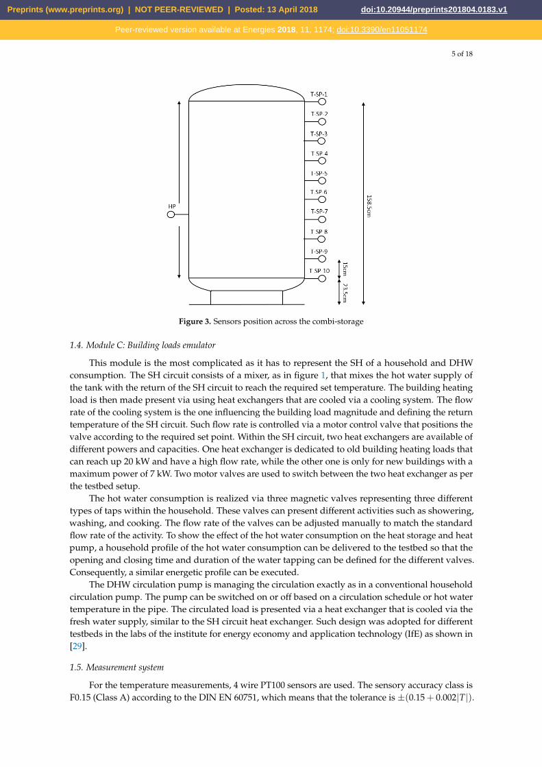
To assess the energetic content of the buffer storage over time, 10 temperature sensors are placedover the length of the tank as shown in figure 3. T-SP-1 refers to the sensor on the top of the tank, whileT-SP-10 refers to the sensor at the bottom of the tank. The sensors are placed at equidistant distances of15 cm. Through this sensors’ set, the energy at each layer of the tank as well as the overall tank contentcan be evaluated. This data represents a necessary input to the energy management systems (EMS)and control algorithms to decide on the load shifting potential and the available flexibility that can beoffered to the grid. Further information about the storage management system can be found in [28]. onthe left side, the heat pump buffer sensor is installed. According to the installation manual of the heatpump, this sensor has to be placed at the bottom of the tank. Within this paper, the sensor position willvary to show its influence on the system performance as shown in section 2. It will be referred to as theDHW/SH sensor.

Preprints (www.preprints.org) | NOT PEER-REVIEWED | Posted: 13 April 2018 doi:10.20944/preprints201804.0183.v1

Peer-reviewed version available at Energies 2018, 11, 1174; doi:10.3390/en11051174

5 of 18

Figure 3. Sensors position across the combi-storage

1.4. Module C: Building loads emulator

This module is the most complicated as it has to represent the SH of a household and DHWconsumption. The SH circuit consists of a mixer, as in figure 1, that mixes the hot water supply ofthe tank with the return of the SH circuit to reach the required set temperature. The building heatingload is then made present via using heat exchangers that are cooled via a cooling system. The flowrate of the cooling system is the one influencing the building load magnitude and defining the returntemperature of the SH circuit. Such flow rate is controlled via a motor control valve that positions thevalve according to the required set point. Within the SH circuit, two heat exchangers are available ofdifferent powers and capacities. One heat exchanger is dedicated to old building heating loads thatcan reach up 20 kW and have a high flow rate, while the other one is only for new buildings with amaximum power of 7 kW. Two motor valves are used to switch between the two heat exchanger as perthe testbed setup.

The hot water consumption is realized via three magnetic valves representing three differenttypes of taps within the household. These valves can present different activities such as showering,washing, and cooking. The flow rate of the valves can be adjusted manually to match the standardflow rate of the activity. To show the effect of the hot water consumption on the heat storage and heatpump, a household profile of the hot water consumption can be delivered to the testbed so that theopening and closing time and duration of the water tapping can be defined for the different valves.Consequently, a similar energetic profile can be executed.

The DHW circulation pump is managing the circulation exactly as in a conventional householdcirculation pump. The pump can be switched on or off based on a circulation schedule or hot watertemperature in the pipe. The circulated load is presented via a heat exchanger that is cooled via thefresh water supply, similar to the SH circuit heat exchanger. Such design was adopted for differenttestbeds in the labs of the institute for energy economy and application technology (IfE) as shown in[29].

1.5. Measurement system

For the temperature measurements, 4 wire PT100 sensors are used. The sensory accuracy class isF0.15 (Class A) according to the DIN EN 60751, which means that the tolerance is ±(0.15 + 0.002|T|).

Preprints (www.preprints.org) | NOT PEER-REVIEWED | Posted: 13 April 2018 doi:10.20944/preprints201804.0183.v1

Peer-reviewed version available at Energies 2018, 11, 1174; doi:10.3390/en11051174

6 of 18

Hence, for a temperature T of 65◦C, the tolerance is ±0.28 ◦C. To maximize the accuracy further, atemperature sensor calibration device of a higher accuracy was used.

Magnetic inductive flow measurements devices are used to measure the volume flow rate. Theflow measurements devices were already calibrated by the manufacturer, consequently no additionalcalibration was performed. For the nominal flow rate, the error of the devices varied between 0.2%and 0.5% depending on the sensor type and the size of the pipe.

The electrical power of the heat pump is measured via a 3-phase electricity meter (KDK PRO380) of class B accuracy, which is 1% according to the EN 50470-1/3. The meter is connected to themeasurement system via MODBUS RTU connection, that communicates the power, currents, andvoltages of the 3 phases each second.

The sensors and actuators of the whole testbed are connected to National instruments (NI)compact reconfigurable IO (cRIO) chassis and modules that receive and send different digital or analoginputs and outputs. The control program and data logger are based on LabVIEW that runs on aconventional PC.

1.6. System and control dynamics

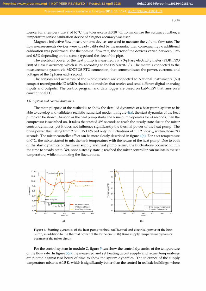
The main purpose of the testbed is to show the detailed dynamics of a heat pump system to beable to develop and validate a realistic numerical model. In figure 4(a), the start dynamics of the heatpump can be shown. As soon as the heat pump starts, the brine pump operates for 24 seconds, then thecompressor is switched on. It takes the testbed 393 seconds to reach the steady state due to the mixercontrol dynamics, yet it does not influence significantly the thermal power of the heat pump. Thebrine power fluctuating from 2.5 till 15.1 kW led only to fluctuations of 10±2.5 kWth, within those 393seconds. The mixer controller effect can be more clearly described in figure 4(b). For a set temperatureof 0◦C, the mixer started to mix the tank temperature with the return of the heat pump. Due to bothof the start dynamics of the mixer supply and heat pump return, the fluctuations occurred withinthe time to steady state. Yet, once a steady state is reached the mixer controller can maintain the settemperature, while minimizing the fluctuations.

0 100 200 300 400 500 600Time [ ]

−5.0

−2.5

0.0

2.5

5.0

7.5

10.0

12.5

15.0

Powe

r [kW

]

Brine pump on

Time to teady-state

HP-Thermal PowerHP-Electrical PowerBrine-Thermal Power

5 10 15 20 250.00.1

(a)

0 100 200 300 400 500 600Time [s]

−7.5

−5.0

−2.5

0.0

2.5

5.0

7.5

10.0

Tempe

rature [°

C]

Brine-Supply TemperatureBrine-Set Temperature

(b)

Figure 4. Starting dynamics of the heat pump testbed, (a)Thermal and electrical power of the heatpump, in addition to the thermal power of the Brine circuit (b) Brine supply temperature dynamicsbecause of the mixer circuit

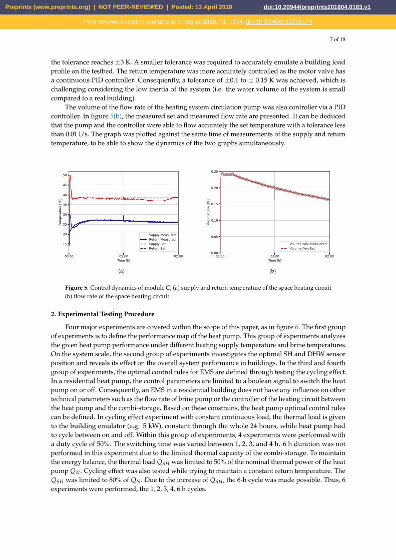
For the control system in module C, figure 5 can show the control dynamics of the temperatureof the flow rate. In figure 5(a), the measured and set heating circuit supply and return temperaturesare plotted against two hours of time to show the system dynamics. The tolerance of the supplytemperature mixer is ±0.5 K, which is significantly better than the control in realistic buildings, where

Preprints (www.preprints.org) | NOT PEER-REVIEWED | Posted: 13 April 2018 doi:10.20944/preprints201804.0183.v1

Peer-reviewed version available at Energies 2018, 11, 1174; doi:10.3390/en11051174

7 of 18

the tolerance reaches ±3 K. A smaller tolerance was required to accurately emulate a building loadprofile on the testbed. The return temperature was more accurately controlled as the motor valve hasa continuous PID controller. Consequently, a tolerance of ±0.1 to ± 0.15 K was achieved, which ischallenging considering the low inertia of the system (i.e. the water volume of the system is smallcompared to a real building).

The volume of the flow rate of the heating system circulation pump was also controller via a PIDcontroller. In figure 5(b), the measured set and measured flow rate are presented. It can be deducedthat the pump and the controller were able to flow accurately the set temperature with a tolerance lessthan 0.01 l/s. The graph was plotted against the same time of measurements of the supply and returntemperature, to be able to show the dynamics of the two graphs simultaneously.

00:00 01:00 02:00Time [h]

15

20

25

30

35

40

45

50

Tempe

rature [°

C]

Supply-MeasuredReturn-MeasuredSupply-Set Return-Set

(a)

00:00 01:00 02:00Time [h]

0.00

0.05

0.10

0.15

0.20

0.25

Volume flo

w [l/s]

Volume flow-MeasureedVolume flow-Set

(b)

Figure 5. Control dynamics of module C, (a) supply and return temperature of the space heating circuit(b) flow rate of the space heating circuit

2. Experimental Testing Procedure

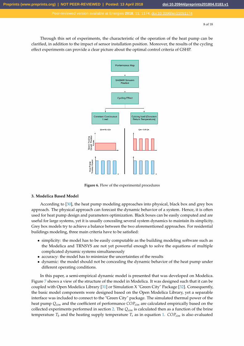
Four major experiments are covered within the scope of this paper, as in figure 6. The first groupof experiments is to define the performance map of the heat pump. This group of experiments analyzesthe given heat pump performance under different heating supply temperature and brine temperatures.On the system scale, the second group of experiments investigates the optimal SH and DHW sensorposition and reveals its effect on the overall system performance in buildings. In the third and fourthgroup of experiments, the optimal control rules for EMS are defined through testing the cycling effect.In a residential heat pump, the control parameters are limited to a boolean signal to switch the heatpump on or off. Consequently, an EMS in a residential building does not have any influence on othertechnical parameters such as the flow rate of brine pump or the controller of the heating circuit betweenthe heat pump and the combi-storage. Based on these constrains, the heat pump optimal control rulescan be defined. In cycling effect experiment with constant continuous load, the thermal load is givento the building emulator (e.g. 5 kW), constant through the whole 24 hours, while heat pump hadto cycle between on and off. Within this group of experiments, 4 experiments were performed witha duty cycle of 50%. The switching time was varied between 1, 2, 3, and 4 h. 6 h duration was notperformed in this experiment due to the limited thermal capacity of the combi-storage. To maintainthe energy balance, the thermal load QSH was limited to 50% of the nominal thermal power of the heatpump QN . Cycling effect was also tested while trying to maintain a constant return temperature. TheQSH was limited to 80% of QN . Due to the increase of QSH , the 6-h cycle was made possible. Thus, 6experiments were performed, the 1, 2, 3, 4, 6 h cycles.

Preprints (www.preprints.org) | NOT PEER-REVIEWED | Posted: 13 April 2018 doi:10.20944/preprints201804.0183.v1

Peer-reviewed version available at Energies 2018, 11, 1174; doi:10.3390/en11051174

8 of 18

Through this set of experiments, the characteristic of the operation of the heat pump can beclarified, in addition to the impact of sensor installation position. Moreover, the results of the cyclingeffect experiments can provide a clear picture about the optimal control criteria of GSHP.

Figure 6. Flow of the experimental procedures

3. Modelica Based Model

According to [30], the heat pump modeling approaches into physical, black box and grey boxapproach. The physical approach can forecast the dynamic behavior of a system. Hence, it is oftenused for heat pump design and parameters optimization. Black boxes can be easily computed and areuseful for large systems, yet it is usually concealing several system dynamics to maintain its simplicity.Grey box models try to achieve a balance between the two aforementioned approaches. For residentialbuildings modeling, three main criteria have to be satisfied:

• simplicity: the model has to be easily computable as the building modeling software such asthe Modelica and TRNSYS are not yet powerful enough to solve the equations of multiplecomplicated dynamic systems simultaneously

• accuracy: the model has to minimize the uncertainties of the results• dynamic: the model should not be concealing the dynamic behavior of the heat pump under

different operating conditions.

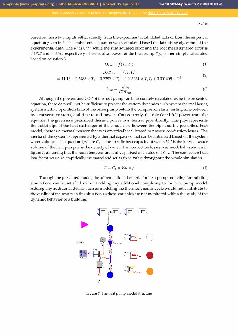
In this paper, a semi-empirical dynamic model is presented that was developed on Modelica.Figure 7 shows a view of the structure of the model in Modelica. It was designed such that it can becoupled with Open Modelica Library [31] or Simulation X "Green City" Package [32]. Consequently,the basic model components were designed based on the Open Modelica Library, yet a separableinterface was included to connect to the "Green City" package. The simulated thermal power of theheat pump Qsim and the coefficient of performance COPsim are calculated empirically based on thecollected experiments performed in section 2. The Qsim is calculated then as a function of the brinetemperature Tb and the heating supply temperature Ts as in equation 1. COPsim is also evaluated

Preprints (www.preprints.org) | NOT PEER-REVIEWED | Posted: 13 April 2018 doi:10.20944/preprints201804.0183.v1

Peer-reviewed version available at Energies 2018, 11, 1174; doi:10.3390/en11051174

9 of 18

based on those two inputs either directly from the experimental tabulated data or from the empiricalequation given in 2. This polynomial equation was formulated based on data fitting algorithm of theexperimental data. The R2 is 0.99, while the sum squared error and the root mean squared error is0.1727 and 0.0759, respectively. The electrical power of the heat pump Psim is then simply calculatedbased on equation 3.

Qsim = f (Tb, Ts) (1)

COPsim = f (Tb, Ts)

= 11.16 + 0.2488× Tb − 0.2282× Ts − 0.003031× TbTs + 0.001405× T2s

(2)

Psim =Qsim

COPsim(3)

Although the powers and COP of the heat pump can be accurately calculated using the presentedequation, these data will not be sufficient to present the system dynamics such system thermal losses,system inertial, operation time of the brine pump before the compressor starts, resting time betweentwo consecutive starts, and time to full power. Consequently, the calculated full power from theequation 1 is given as a prescribed thermal power to a thermal pipe directly. This pipe representsthe outlet pipe of the heat exchanger of the condenser. Between the pipe and the prescribed heatmodel, there is a thermal resistor that was empirically calibrated to present conduction losses. Theinertia of the system is represented by a thermal capacitor that can be initialized based on the systemwater volume as in equation 4,where Cp is the specific heat capacity of water, Vol is the internal watervolume of the heat pump, ρ is the density of water. The convection losses was modeled as shown infigure 7, assuming that the room temperature is always fixed at a value of 18 ◦C. The convection heatloss factor was also empirically estimated and set as fixed value throughout the whole simulation.

C = Cp ×Vol × ρ (4)

Through the presented model, the aforementioned criteria for heat pump modeling for buildingsimulations can be satisfied without adding any additional complexity to the heat pump model.Adding any additional details such as modeling the thermodynamic cycle would not contribute tothe quality of the results in this situation as these variables are not monitored within the study of thedynamic behavior of a building.

Figure 7. The heat pump model structure

Preprints (www.preprints.org) | NOT PEER-REVIEWED | Posted: 13 April 2018 doi:10.20944/preprints201804.0183.v1

Peer-reviewed version available at Energies 2018, 11, 1174; doi:10.3390/en11051174

10 of 18

4. Results

4.1. Experimental Analysis

4.1.1. System Performance

As explained in section 2, the initial phase of the experimental study is to analyze the performancemap of the given heat pump. Figure 8 shows the behavior of the COP as a function of the supplytemperature and the brine temperature. At each of the measured points of Tb and Ts, the set pointswere held constant and measurement was taken as an average of 40 minutes of operation to maintain aproper steady and accurate measurements. The set points are defined as a discrete set of integers suchthat Ts ∈ {35, 40, 45, 50, 55, 60, 65} and Tb ∈ {−5, 0, 10, 15, 20}. In figure 8, the measurements at 65◦Cwas eliminated, as the heat pump can not operate at Tb = −5 and Ts = 65 simultaneously. As shown,the COP increases as the supply temperature decrease and the brine temperature increases. The rangeof the COP is quite wide between 1.6 and 8.0. This means that the costs of operation of the heat pumpto generate 1 kWh of heat can reach up to 500% compared to the cost of the most optimal possibleoperation. Consequently, it is a must to supply the numerical models with an accurate measured data,otherwise building model can be exposed to high uncertainties.

−5 0 5 10 15Brine temperature [°C]

35

40

45

50

55

60

Supp

ly te

mpe

rature [°

C]

1.6

2.4

3.2

4.0

4.8

5.6

6.4

7.2

8.0COP

Figure 8. Performance map of the integrated GSHP

4.1.2. Sensors Position

System setup and configuration in the building has also a significant influence on the behaviorof the COP of the heat pump. In the field study of [12], the impact of an efficient planning andinstallation on the heat pump seasonal performance factor was investigated. The installation processdoes not only include hydraulic system but also the DWH and SH sensors positioning on the storagesystem. Although direct connection of the SH circuit to the buildings without any buffer storage canlead to the most optimal operation, buffer storages are necessary to offer flexibility as in [33]. In theliterature, different research discussed the sensor position. In [11], different sensors positions alonga combi-storage were tested based on a simulation model. It was found that as the DHW sensorsdistances from the SH zone, the lower is the number of starts per year. In [26,34], it was stated thatthe DHW sensor has no influence on the performance of the heat pump, yet the higher the positionthe better. Moreover, the author stated that sensors at a lower position can help in decreasing the settemperature while maintaining comfort.

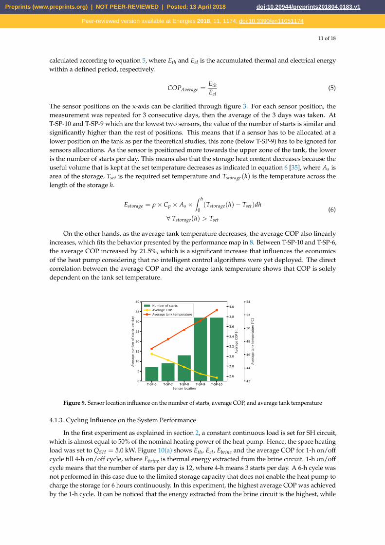
Within this experimental study, one sensor was set in different position across the combi-storageto analyze the behavior of the heat pump and the heat storage as well. Additional sensors connectionto the control of the heat pump manufacturer was not possible. Figure 9 shows the average number ofstarts, average COP and average tank temperature at different sensors positions. The average COP is

Preprints (www.preprints.org) | NOT PEER-REVIEWED | Posted: 13 April 2018 doi:10.20944/preprints201804.0183.v1

Peer-reviewed version available at Energies 2018, 11, 1174; doi:10.3390/en11051174

11 of 18

calculated according to equation 5, where Eth and Eel is the accumulated thermal and electrical energywithin a defined period, respectively.

COPAverage =EthEel

(5)

The sensor positions on the x-axis can be clarified through figure 3. For each sensor position, themeasurement was repeated for 3 consecutive days, then the average of the 3 days was taken. AtT-SP-10 and T-SP-9 which are the lowest two sensors, the value of the number of starts is similar andsignificantly higher than the rest of positions. This means that if a sensor has to be allocated at alower position on the tank as per the theoretical studies, this zone (below T-SP-9) has to be ignored forsensors allocations. As the sensor is positioned more towards the upper zone of the tank, the loweris the number of starts per day. This means also that the storage heat content decreases because theuseful volume that is kept at the set temperature decreases as indicated in equation 6 [35], where As isarea of the storage, Tset is the required set temperature and Tstorage(h) is the temperature across thelength of the storage h.

Estorage = ρ× Cp × As ×∫ h

0(Tstorage(h)− Tset)dh

∀ Tstorage(h) > Tset

(6)

On the other hands, as the average tank temperature decreases, the average COP also linearlyincreases, which fits the behavior presented by the performance map in 8. Between T-SP-10 and T-SP-6,the average COP increased by 21.5%, which is a significant increase that influences the economicsof the heat pump considering that no intelligent control algorithms were yet deployed. The directcorrelation between the average COP and the average tank temperature shows that COP is solelydependent on the tank set temperature.

T-SP-6 T-SP-7 T-SP-8 T-SP-9 T-SP-10Sensor location

0

5

10

15

20

25

30

35

40

Average number of starts per day

7 9 13 32322.6

2.8

3.0

3.2

3.4

3.6

3.8

4.0

Average COP [-]

Number of startsAverage COPAverage tank temperature

42

44

46

48

50

52

54

Average tank temperature [°C]

Figure 9. Sensor location influence on the number of starts, average COP, and average tank temperature

4.1.3. Cycling Influence on the System Performance

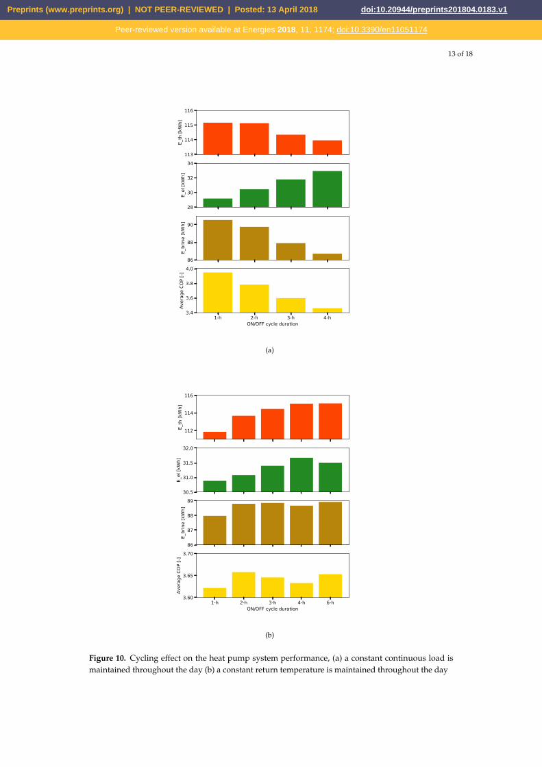
In the first experiment as explained in section 2, a constant continuous load is set for SH circuit,which is almost equal to 50% of the nominal heating power of the heat pump. Hence, the space heatingload was set to QSH = 5.0 kW. Figure 10(a) shows Eth, Eel , Ebrine and the average COP for 1-h on/offcycle till 4-h on/off cycle, where Ebrine is thermal energy extracted from the brine circuit. 1-h on/offcycle means that the number of starts per day is 12, where 4-h means 3 starts per day. A 6-h cycle wasnot performed in this case due to the limited storage capacity that does not enable the heat pump tocharge the storage for 6 hours continuously. In this experiment, the highest average COP was achievedby the 1-h cycle. It can be noticed that the energy extracted from the brine circuit is the highest, while

Preprints (www.preprints.org) | NOT PEER-REVIEWED | Posted: 13 April 2018 doi:10.20944/preprints201804.0183.v1

Peer-reviewed version available at Energies 2018, 11, 1174; doi:10.3390/en11051174

12 of 18

the electricity consumed is the lowest. The heat generated is almost constant. It has varied onlybetween 113.85 kWh to 115.2.

Although 1-h cycle has the highest number of starts, it achieved the highest COP because itmaintained the lowest possible tank temperature. Having the heat pump operating for 4 hours thenstopping for 4 hours while having a constant demand from the SH circuit means that the heat pumphas to heat the buffer storage to higher temperatures to satisfy the demand during the off (i.e. restingtime). Although the 4-h cycle minimized the number of starts to only 3 times per day, it does not leadto an optimal efficient operation. The average COP was lowered by 13%. The lower number of startsmight increase the lifetime of the compressor, yet this is not a measurable factor that can be assessedeasily by a testbed or even within a field study at the moment. If it would be included, a cost of starthas to be evaluated to reach an optimal control schedule.

In the second experiment, the QSH was increased to 8 kW and the QSH was not set to becontinuous, but cycling similar to the heat pump. The reason behind increasing the power of the loadand the simultaneous cycling is to consume immediately the delivered power of the heat pump and tomaintain the lowest possible return temperature Tr. In this case, 1-h to 6-h cycles were used as theheat storage was almost not used. Through this experiment, it can be noticed that the average COP isalmost constant and was not influenced by either the long or short duration of heat pump operation.The energies Eth, Eel , and Ebrine varied only by 2.7%, 1.5% and 1.136 %, respectively. Such variationis partially due to the measurement errors and the minor difference in the initial conditions of theexperiment.

To summarize the output of these experiments, it can be deduced that if a buffer or combi-storageare combined with the heat pump:

• The long operation duration to minimize the heat pump number of starts reduces the averageCOP and consequently can lead to a lower seasonal performance factor (SPF)• If the heat pump is delivering directly while minimally using the heat storage or without a heat

storage, the long duration of operation has no impact on the average COP of the system

Consequently, if a combi-storage has to be installed to minimize the number of starts per day, acost of start has to be considered within the optimization. In case the heat pump has to offer flexibilityto the grid, the incentives should be making up for the decrease in COP that can lead in this case to aminimum of 13% increase in costs. Additionally, thermal losses of the storage have to be considered.

Preprints (www.preprints.org) | NOT PEER-REVIEWED | Posted: 13 April 2018 doi:10.20944/preprints201804.0183.v1

Peer-reviewed version available at Energies 2018, 11, 1174; doi:10.3390/en11051174

13 of 18

113

114

115

116

E_th [k

Wh]

28

30

32

34

E_el [k

Wh]

86

88

90

E_brine [kWh]

1-h 2-h 3-h 4-hON/OFF cycle duration

3.4

3.6

3.8

4.0

Averag

e CO

P [-]

(a)

112

114

116

E_th

[kW

h]

30.5

31.0

31.5

32.0

E_el

[kW

h]

86

87

88

89

E_br

ine

[kW

h]

1-h 2-h 3-h 4-h 6-hON/OFF cycle duration

3.60

3.65

3.70

Aver

age

COP

[-]

(b)

Figure 10. Cycling effect on the heat pump system performance, (a) a constant continuous load ismaintained throughout the day (b) a constant return temperature is maintained throughout the day

Preprints (www.preprints.org) | NOT PEER-REVIEWED | Posted: 13 April 2018 doi:10.20944/preprints201804.0183.v1

Peer-reviewed version available at Energies 2018, 11, 1174; doi:10.3390/en11051174

14 of 18

4.2. Model Validation

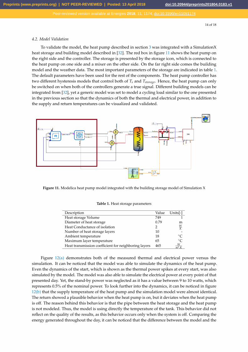
To validate the model, the heat pump described in section 3 was integrated with a SimulationXheat storage and building model described in [32]. The red box in figure 11 shows the heat pump onthe right side and the controller. The storage is presented by the storage icon, which is connected tothe heat pump on one side and a mixer on the other side. On the far right side comes the buildingmodel and the weather data. The most important parameters of the storage are indicated in table 1.The default parameters have been used for the rest of the components. The heat pump controller hastwo different hysteresis models that control both of Ts and Tstorage. Hence, the heat pump can onlybe switched on when both of the controllers generate a true signal. Different building models can beintegrated from [32], yet a generic model was set to model a cycling load similar to the one presentedin the previous section so that the dynamics of both the thermal and electrical power, in addition tothe supply and return temperatures can be visualized and validated.

Figure 11. Modelica heat pump model integrated with the building storage model of Simulation X

Table 1. Heat storage parameters

Description Value Units[-]Heat storage Volume 749 lDiameter of heat storage 0.79 mHeat Conductance of isolation 2 W

KNumber of heat storage layers 10 -Ambient temperature 18 ◦CMaximum layer temperature 65 ◦CHeat transmission coefficient for neighboring layers 465 W

m2.K

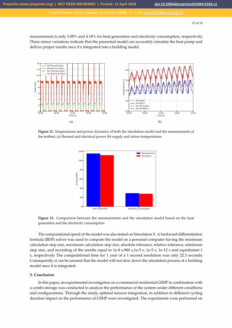
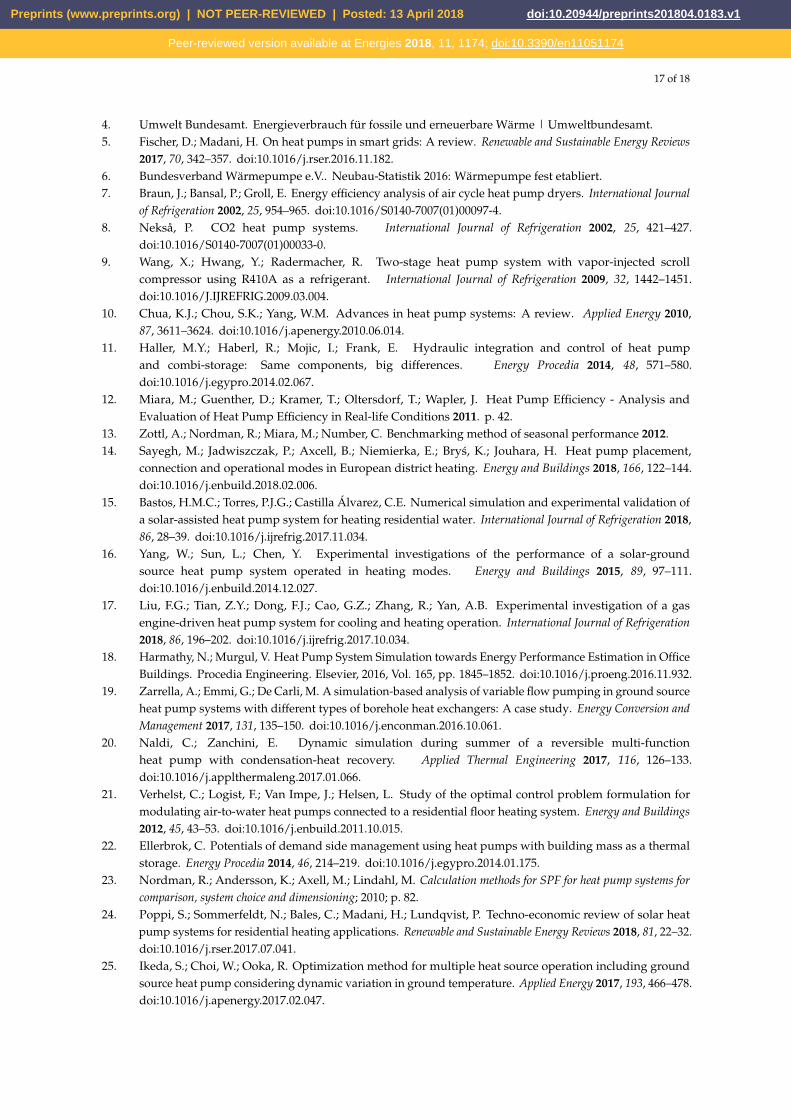
Figure 12(a) demonstrates both of the measured thermal and electrical power versus thesimulation. It can be noticed that the model was able to simulate the dynamics of the heat pump.Even the dynamics of the start, which is shown as the thermal power spikes at every start, was alsosimulated by the model. The model was also able to simulate the electrical power at every point of thatpresented day. Yet, the stand-by power was neglected as it has a value between 9 to 10 watts, whichrepresents 0.5% of the nominal power. To look further into the dynamics, it can be noticed in figure12(b) that the supply temperature of the heat pump and the simulation model were almost identical.The return showed a plausible behavior when the heat pump is on, but it deviates when the heat pumpis off. The reason behind this behavior is that the pipe between the heat storage and the heat pumpis not modeled. Thus, the model is using directly the temperature of the tank. This behavior did notreflect on the quality of the results, as this behavior occurs only when the system is off. Comparing theenergy generated throughout the day, it can be noticed that the difference between the model and the

Preprints (www.preprints.org) | NOT PEER-REVIEWED | Posted: 13 April 2018 doi:10.20944/preprints201804.0183.v1

Peer-reviewed version available at Energies 2018, 11, 1174; doi:10.3390/en11051174

15 of 18

measurement is only 3.08% and 4.18% for heat generation and electricity consumption, respectively.These minor variations indicate that the presented model can accurately simulate the heat pump anddeliver proper results once it’s integrated into a building model.

00:00 06:00 12:00 18:00 23:59Time [h]

0

2

4

6

8

10

12

14

16

Powe

r [kW

]

HP-Thermal PowerHP-Electrical PowerSim-Thermal PowerSim-Electrical Power

(a)

00:00 06:00 12:00 18:00 23:59Time [h]

20

25

30

35

40

Tempe

ratu

re [°

C]

HP SupplyHP ReturnSim-HP SupplySim-HP Return

(b)

Figure 12. Temperatures and power dynamics of both the simulation model and the measurements ofthe testbed, (a) thermal and electrical power (b) supply and return temperatures

Heat Generation Electricity Consumption0

20

40

60

80

100

120

Energy

[kWh]

MeasurementSimulation

Figure 13. Comparison between the measurements and the simulation model based on the heatgeneration and the electricity consumption

The computational speed of the model was also tested on Simulation X. A backward differentiationformula (BDF) solver was used to compute the model on a personal computer having the minimumcalculation step size, maximum calculation step size, absolute tolerance, relative tolerance, minimumstep size, and recording of the results equal to 1e-8 s,900 s,1e-5 s, 1e-5 s, 1e-12 s and equidistant 1s, respectively The computational time for 1 year of a 1 second resolution was only 22.3 seconds.Consequently, it can be assured that the model will not slow down the simulation process of a buildingmodel once it is integrated.

5. Conclusion

In this paper, an experimental investigation on a commercial residential GSHP in combination witha combi-storage was conducted to analyze the performance of the system under different conditionsand configurations. Through the study, optimal sensors integration, in addition to different cyclingduration impact on the performance of GSHP were investigated. The experiments were performed on

Preprints (www.preprints.org) | NOT PEER-REVIEWED | Posted: 13 April 2018 doi:10.20944/preprints201804.0183.v1

Peer-reviewed version available at Energies 2018, 11, 1174; doi:10.3390/en11051174

16 of 18

a modular testbed that can emulate the behavior of the ground source, as it can deliver a profile ofbrine temperatures in real-time. Moreover, it can emulate loads of space heating and domestic hotwater consumption for different building sizes and ages. Through the experimental investigation itcan be concluded the following:

• SH/DHW sensor position influence the number of starts and might lead to short cycling, yet it isnot the main parameter influencing the COP• Tank set temperature has a direct impact on COP. Thus, for the same required supply temperature,

having a sensor at a higher position along with a high set temperature could be exactly equal tohaving the sensor at a lower position with a low set temperature• Having short cycles do not always lead to a lower COP, it can actually increase the average COP

of the system as it maintains a lower temperature in the tank• In case the heat pump is delivering directly to the building without a storage or once there is a

consumption from storage, the long or short cycles do not have an impact on the COP• Higher number of starts might lead to a shorter life for the compressor, consequently, a cost of

start has to be included to balance the benefit of the higher COP with short cycles. Otherwise,the EMS might tend to increase the number of starts per day of the heat pump, if no flexibility isrequired from the grid

The aforementioned experimental data was used to develop a Modelica model that can accuratelymodel the dynamics and behavior of the heat pump. Comparing the daily energy consumption of themeasurements of the testbed to the model, it was found that the difference in heat generation and theelectricity consumption is only 3% and 4%, respectively. Moreover, the model can be easily solved fora 1-year time horizon of one-second resolution in 22.3 seconds on a personal computer. Thus, it can beeasily integrated into a complete building model without slowing down the solver.

The developed testbed opens the horizon towards several other investigations and demonstrationof multiple methods. As a next step, it is planned to integrate the testbed as part of a hardware in theloop (HiL) system as presented in [36]. Through that HiL system, a communication can be performedwith different models to emulate real-life conditions.

6. Acknowledgment

This work was supported by the German Research Foundation (DFG) and the Technical Universityof Munich within the Open Access Publishing Funding Program. The research project is supported bythe Federal Ministry for Economic Affairs and Energy, Bundesministerium für Wirtschaft und Energie,as a part of the SINTEG project C/sells. Responsibility for the content of this publication lies on theauthors.

7. Author Contributions

Wessam El-Baz designed the experiments and the model. Peter Tzscheutschler and Ulrich Wagnerprovided a detailed critical review. All the authors discussed the documents results and contributed tothe preparation of the manuscript.

8. Conflicts of Interest

The authors declare no conflict of interest

References

1. Bundesministrium für Wirtschaft und Energie. BMWi - Erneuerbare Energien.2. Wüstenhagen, R.; Bilharz, M. Green energy market development in Germany: effective public policy and

emerging customer demand. Energy Policy 2006, 34, 1681–1696. doi:10.1016/j.enpol.2004.07.013.3. Bloess, A.; Schill, W.P.; Zerrahn, A. Power-to-heat for renewable energy integration: A review of

technologies, modeling approaches, and flexibility potentials. Applied Energy 2018, 212, 1611–1626.doi:10.1016/j.apenergy.2017.12.073.

Preprints (www.preprints.org) | NOT PEER-REVIEWED | Posted: 13 April 2018 doi:10.20944/preprints201804.0183.v1

Peer-reviewed version available at Energies 2018, 11, 1174; doi:10.3390/en11051174

17 of 18

4. Umwelt Bundesamt. Energieverbrauch für fossile und erneuerbare Wärme | Umweltbundesamt.5. Fischer, D.; Madani, H. On heat pumps in smart grids: A review. Renewable and Sustainable Energy Reviews

2017, 70, 342–357. doi:10.1016/j.rser.2016.11.182.6. Bundesverband Wärmepumpe e.V.. Neubau-Statistik 2016: Wärmepumpe fest etabliert.7. Braun, J.; Bansal, P.; Groll, E. Energy efficiency analysis of air cycle heat pump dryers. International Journal

of Refrigeration 2002, 25, 954–965. doi:10.1016/S0140-7007(01)00097-4.8. Nekså, P. CO2 heat pump systems. International Journal of Refrigeration 2002, 25, 421–427.

doi:10.1016/S0140-7007(01)00033-0.9. Wang, X.; Hwang, Y.; Radermacher, R. Two-stage heat pump system with vapor-injected scroll

compressor using R410A as a refrigerant. International Journal of Refrigeration 2009, 32, 1442–1451.doi:10.1016/J.IJREFRIG.2009.03.004.

10. Chua, K.J.; Chou, S.K.; Yang, W.M. Advances in heat pump systems: A review. Applied Energy 2010,87, 3611–3624. doi:10.1016/j.apenergy.2010.06.014.

11. Haller, M.Y.; Haberl, R.; Mojic, I.; Frank, E. Hydraulic integration and control of heat pumpand combi-storage: Same components, big differences. Energy Procedia 2014, 48, 571–580.doi:10.1016/j.egypro.2014.02.067.

12. Miara, M.; Guenther, D.; Kramer, T.; Oltersdorf, T.; Wapler, J. Heat Pump Efficiency - Analysis andEvaluation of Heat Pump Efficiency in Real-life Conditions 2011. p. 42.

13. Zottl, A.; Nordman, R.; Miara, M.; Number, C. Benchmarking method of seasonal performance 2012.14. Sayegh, M.; Jadwiszczak, P.; Axcell, B.; Niemierka, E.; Brys, K.; Jouhara, H. Heat pump placement,

connection and operational modes in European district heating. Energy and Buildings 2018, 166, 122–144.doi:10.1016/j.enbuild.2018.02.006.

15. Bastos, H.M.C.; Torres, P.J.G.; Castilla Álvarez, C.E. Numerical simulation and experimental validation ofa solar-assisted heat pump system for heating residential water. International Journal of Refrigeration 2018,86, 28–39. doi:10.1016/j.ijrefrig.2017.11.034.

16. Yang, W.; Sun, L.; Chen, Y. Experimental investigations of the performance of a solar-groundsource heat pump system operated in heating modes. Energy and Buildings 2015, 89, 97–111.doi:10.1016/j.enbuild.2014.12.027.

17. Liu, F.G.; Tian, Z.Y.; Dong, F.J.; Cao, G.Z.; Zhang, R.; Yan, A.B. Experimental investigation of a gasengine-driven heat pump system for cooling and heating operation. International Journal of Refrigeration2018, 86, 196–202. doi:10.1016/j.ijrefrig.2017.10.034.

18. Harmathy, N.; Murgul, V. Heat Pump System Simulation towards Energy Performance Estimation in OfficeBuildings. Procedia Engineering. Elsevier, 2016, Vol. 165, pp. 1845–1852. doi:10.1016/j.proeng.2016.11.932.

19. Zarrella, A.; Emmi, G.; De Carli, M. A simulation-based analysis of variable flow pumping in ground sourceheat pump systems with different types of borehole heat exchangers: A case study. Energy Conversion andManagement 2017, 131, 135–150. doi:10.1016/j.enconman.2016.10.061.

20. Naldi, C.; Zanchini, E. Dynamic simulation during summer of a reversible multi-functionheat pump with condensation-heat recovery. Applied Thermal Engineering 2017, 116, 126–133.doi:10.1016/j.applthermaleng.2017.01.066.

21. Verhelst, C.; Logist, F.; Van Impe, J.; Helsen, L. Study of the optimal control problem formulation formodulating air-to-water heat pumps connected to a residential floor heating system. Energy and Buildings2012, 45, 43–53. doi:10.1016/j.enbuild.2011.10.015.

22. Ellerbrok, C. Potentials of demand side management using heat pumps with building mass as a thermalstorage. Energy Procedia 2014, 46, 214–219. doi:10.1016/j.egypro.2014.01.175.

23. Nordman, R.; Andersson, K.; Axell, M.; Lindahl, M. Calculation methods for SPF for heat pump systems forcomparison, system choice and dimensioning; 2010; p. 82.

24. Poppi, S.; Sommerfeldt, N.; Bales, C.; Madani, H.; Lundqvist, P. Techno-economic review of solar heatpump systems for residential heating applications. Renewable and Sustainable Energy Reviews 2018, 81, 22–32.doi:10.1016/j.rser.2017.07.041.

25. Ikeda, S.; Choi, W.; Ooka, R. Optimization method for multiple heat source operation including groundsource heat pump considering dynamic variation in ground temperature. Applied Energy 2017, 193, 466–478.doi:10.1016/j.apenergy.2017.02.047.

Preprints (www.preprints.org) | NOT PEER-REVIEWED | Posted: 13 April 2018 doi:10.20944/preprints201804.0183.v1

Peer-reviewed version available at Energies 2018, 11, 1174; doi:10.3390/en11051174

18 of 18

26. Glembin, J.; Büttner, C.; Steinweg, J.; Rockendorf, G. Optimal Connection of Heat Pump andSolar Buffer Storage under Different Boundary Conditions. Energy Procedia 2016, 91, 145–154.doi:10.1016/j.egypro.2016.06.190.

27. Le, K.X.; Shah, N.; Huang, M.J.; Hewitt, N.J. High Temperature Air-Water Heat Pump and Energy Storage :Validation of TRNSYS Models 2017. II.

28. Wehmhörner, U. Multikriterielle Regelung mit temperaturbasierter Speicherzustandsbestimmung fürMini-KWK-Anlagen 2012.

29. Mühlbacher, H. Verbrauchsverhalten von Wärmeerzeugern bei dynamisch variierten Lasten undÜbertragungskomponenten 2007. p. 127.

30. Ljubijankic, M.; Nytsch-Geusen, C.; Rädler, J.; Löffler, M. Numerical coupling of Modelica and CFD forbuilding energy supply systems. Proceedings of the 8th International Modelica Conference 2011, pp. 286–294.

31. Open Modelica. OpenModelica.32. ESI ITI. SimulationX 3.8 | Green City.33. El-Baz, W.; Tzscheutschler, P. Autonomous Coordination of Smart Buildings in Microgrids based on a

Double-Sided Auction. IEEE Power and Energy Society General Meeting; , 2017; Number August.34. Glembin, J.; Büttner, C.; Steinweg, J.; Rockendorf, G. Thermal storage tanks in high efficiency heat pump

systems - Optimized installation and operation parameters. Energy Procedia. Elsevier B.V., 2015, Vol. 73,pp. 331–340. doi:10.1016/j.egypro.2015.07.700.

35. Lipp, J.; Sänger, F. Potential of power shifting using a micro-CHP units and heat storages; Microgen3:Naples, Italy, 2013.

36. El-Baz, W.; Sänger, F.; Tzscheutschler, P. HARDWARE IN THE LOOP ( HIL ) FOR MICRO CHP SYSTEMS.The Fourth Internatinal Conference on Microgeneration and related Technologies; Microgen4: Tokyo,Japan, 2015.

Preprints (www.preprints.org) | NOT PEER-REVIEWED | Posted: 13 April 2018 doi:10.20944/preprints201804.0183.v1

Peer-reviewed version available at Energies 2018, 11, 1174; doi:10.3390/en11051174