Embed Size (px)
Citation preview
0369-000017
Experimental Studies of Viscous Loss in a Hydraulic Flywheel Accumulator
Kyle G. Strohmaier, Paul M. Cronk, Anthony L. Knutson, James D. Van de Ven, Ph.D. University of Minnesota-Twin Cities
ABSTRACT
The hydraulic flywheel accumulator, a novel hydro-kinetic energy storage device, consists of a piston-style hydraulic accumulator which rotates at high speed about the longitudinal axis. In comparison to traditional accumulator storage, this rotation significantly increases energy density and decouples system pressure from state-of-charge. Angular acceleration during operation causes the fluid within the device to depart from rigid body rotation. It is important to model the resultant three-dimensional flow, as it has implications on viscous energy dissipation and transient response of accumulator pressure. The computational cost of a full CFD simulation makes it undesirable for modeling and optimization. This paper details the development of a simplified quasi-empirical model for fluid behavior in the hydraulic flywheel accumulator.
INTRODUCTION
BACKGROUND
Hydraulics are widely used for power transmission in the agricultural, industrial, aerospace, mining, and construction sectors. The prevalence of hydraulic systems is due largely to the durability, reliability, high power density, and low cost of their components. Traditionally, energy for hydraulic systems is stored pneumatically in an accumulator, which is a pressure vessel containing a gas volume and an oil volume separated by a piston or bladder. Adding or extracting oil charges or discharges the accumulator by compressing or expanding the gas. Traditional hydraulic accumulators are extremely power dense, but have relatively little energy capacity. Current high-performance composite hydraulic accumulators offer an energy density of about
1), two orders of
magnitude lower than advanced electrochemical batteries or advanced flywheels
2). This large
discrepancy makes it difficult for hydraulic power to compete with other technologies in mobile applications with energy regeneration, where energy density is important. In addition to being quite limited in energy density, the utility of a traditional hydraulic accumulator is hindered by the fact that its pressure is coupled to the amount of energy stored. Consequently, all hydraulic system components must be sized for the high flow rates that are required to meet a power demand at low pressure.
The hydraulic flywheel accumulator (HFA) proposed by Van de Ven
3) has the potential to overcome both of the
major drawbacks of a traditional hydraulic accumulator, significantly increasing energy storage density while decoupling system pressure from the state of charge (SOC).
HYDRAULIC FLYWHEEL ACCUMULATOR CONCEPT
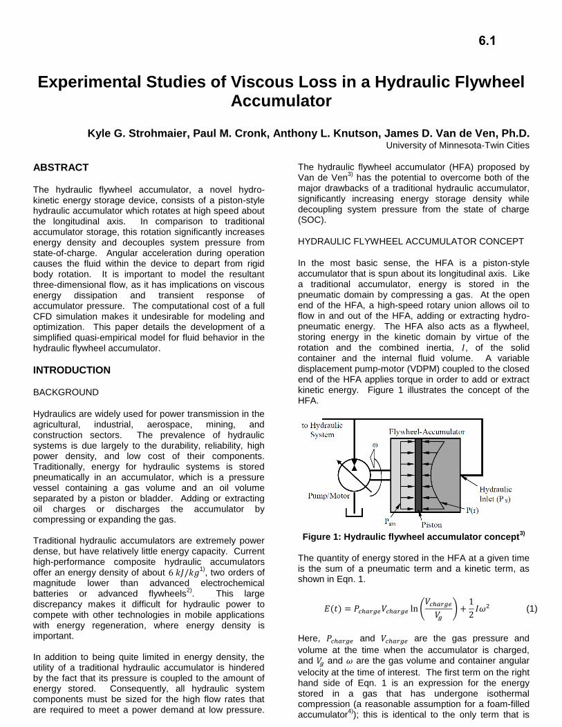
In the most basic sense, the HFA is a piston-style accumulator that is spun about its longitudinal axis. Like a traditional accumulator, energy is stored in the pneumatic domain by compressing a gas. At the open end of the HFA, a high-speed rotary union allows oil to flow in and out of the HFA, adding or extracting hydro-pneumatic energy. The HFA also acts as a flywheel, storing energy in the kinetic domain by virtue of the rotation and the combined inertia, , of the solid container and the internal fluid volume. A variable displacement pump-motor (VDPM) coupled to the closed end of the HFA applies torque in order to add or extract kinetic energy. Figure 1 illustrates the concept of the HFA.
Figure 1: Hydraulic flywheel accumulator concept
3)
The quantity of energy stored in the HFA at a given time is the sum of a pneumatic term and a kinetic term, as shown in Eqn. 1.
(1)
Here, and are the gas pressure and
volume at the time when the accumulator is charged, and and are the gas volume and container angular
velocity at the time of interest. The first term on the right hand side of Eqn. 1 is an expression for the energy stored in a gas that has undergone isothermal compression (a reasonable assumption for a foam-filled accumulator
4)); this is identical to the only term that is
6.1
present in the stored energy equation for a traditional accumulator. The second term in Eqn. 1 is an expression for the kinetic energy stored in a rotating body. Equation 1 is written for steady state, a condition where the fluid volume is rotating as a rigid body at the same angular velocity as the container. The kinetic energy term suggests that increasing the angular velocity of the HFA causes a quadratic increase in the stored kinetic energy without directly affecting the mass of the system. Clearly, then, utilization of the kinetic domain allows for a significant improvement in energy density over traditional accumulator storage. Imposing an angular velocity on the HFA not only increases energy storage density, but also leads to internal fluid phenomena that can be exploited for an additional benefit. A force balance on a fluid element in rigid body rotation yields a radially-dependent parabolic oil pressure distribution
3). The practical result of this
parabolic pressure distribution is that the inlet/outlet pressure, which is at the center of the HFA and is the pressure experienced by the rest of the hydraulic system, is lower than the average pressure of the accumulator. The difference between the average and center pressures is proportional to angular velocity. This concept is expressed mathematically as:
(2)
The parameter refers to system (center) pressure, is fluid density, and is the inner radius of the container. The first term on the right side of the equality represents the average accumulator pressure. Like the stored energy equation (Eqn. 1), Eqn. 2 is written for steady state. All parameters on the right hand sides of both of these equations are constant throughout the HFA operation, except for angular velocity and gas volume. It is therefore useful to consider these two variables as fully describing the operating state. From examination of Eqns. 1 and 2, it is easy to see that the two controllable operating parameters, angular velocity and gas volume, can be independently modulated such that system pressure is decoupled from SOC. MOTIVATION FOR FLUID MODELING In the application of a hydraulic hybrid passenger vehicle, the HFA is subject to an unpredictable and highly transient power profile. Regenerative braking makes energy available for addition to the HFA, while vehicle acceleration and road loads require extraction of energy. The inertial and pressure responses to a transient power profile have implications on performance metrics (eg. energy conversion efficiency, pressure fluctuation) and necessary design features (eg. wall thickness, rated bearing speed). For purposes of design optimization, it is necessary to accurately characterize the dynamic response of the HFA to such a transient power profile.
The simplest way to simulate HFA performance would be to assume the fluid volume behaves as a solid. In this case, the fluid would always be at steady state, rotating as a rigid body at the speed of the container. In modeling inertial behavior, Newton’s second law could be applied simply using the sum of the fluid and solid inertias, and no viscous dissipation would occur. Pressure at the fluid inlet could be inferred at any time by simply measuring the velocity of the container (which, by virtue of the present assumption, would also indicate the velocity of the fluid volume). The assumption that the fluid volume behaves as a solid, where no viscous losses are incurred and pressure responds instantly to a change in container angular velocity, has been used to drive a preliminary design optimization
5). By neglecting fluid behavior and viscous
losses (as well as all other energy loss mechanisms) this study aimed to provide only general insight into what an optimal HFA design might resemble. For a detailed design optimization, however, these phenomena must be included in the performance modeling, and therefore a more thorough understanding of transient fluid behavior is sought. Storing energy in two domains leads to two distinct types of transients. Use of the pneumatic domain requires changing the volume of oil in the HFA. While this certainly results in interesting transient phenomena by altering the inertia of the HFA, it is not the topic of this paper, and therefore constant oil volume is implied in all of the following discussion. This paper instead focuses on modeling the transient fluid behavior resultant from utilizing the kinetic domain. In this mode of energy exchange, the HFA experiences angular acceleration or deceleration by the application of positive or negative torque. Leaving exact details for later discussion, it is intuitive that, as a torque is applied to the container, the fluid volume will not necessarily behave as a solid. Should the container maintain a constant angular velocity for a sufficiently long period of time, the fluid volume will eventually return to steady state. Understanding the nature by which the fluid volume departs from steady state is important for two reasons:
Fluid behavior impacts the applicability of Eqns. 1 and 2 to regions of transient operation
Viscous dissipation of energy occurs whenever the fluid is not rotating as a rigid body
To model transient HFA behavior for any power profile of reasonable duration and temporal resolution, full CFD would result in far too much computational cost. This is especially true in the context of a heuristic design optimization, where the thousands of potential HFA designs must be evaluated via simulation
5). The ideal
model for fluid behavior, therefore, must be accurate enough to realistically predict HFA behavior and computationally cheap enough that simulation and

optimization can be carried out in an reasonable amount of time. The remainder of this paper describes the method by which the desired model is developed. The first section reviews some theory on rotating flows, then puts forth and defends a key assumption for the fluid model. In the next section, the general approach to fluid modeling is presented and a dimensional analysis is carried out. The following section describes the experimental methods and results used to develop the fluid model. The final section mates the theory with the experimental results and provides an evaluation of the model.
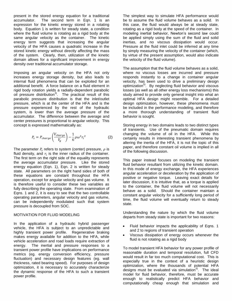
THEORY AND ASSUMPTIONS EKMAN SPIN-UP THEORY A rich body of research, which could be collectively called “Ekman spin-up theory”, provides valuable insight into the expected transient behavior of the fluid volume. Most of the research is a variation on the following theme: An axisymmetric fluid is initially rotating at steady state when its container is impulsively accelerated to a new angular velocity. Generally, the process of fluid spin-down is the reverse of spin-up, so the following brief review of Ekman spin-up theory can be applied to a container which is impulsively accelerated or decelerated. Figure 2 shows a container of finite wall thickness with important dimensions labeled.
Figure 2: Container and fluid volume with
dimensions In the limiting case of an infinitely long ( ) cylindrical fluid volume, any departure from fluid rigid body rotation manifests itself as a two-dimensional flow relative to the container. In this special case, transport of momentum within the fluid is accomplished purely through viscous diffusion. However, for any reasonable set of geometric dimensions, the HFA aspect ratio ( ) is far too low for infinite length to be a suitable approximation
5).
Instead, it turns out that the relative flow during transience is quite three-dimensional (though still axisymmetric), with the end walls playing an extremely important role
6). Due to the no-slip condition, an
impulsive increase in the container angular velocity results in a thin layer of fluid at the walls which rotates faster than the core flow. These thin layers of fluid are subject, then, to a centrifugal field that overcomes the prevailing pressure gradient (the pressure gradient imposed by the rotation of the core flow). Consequently, fluid at the end walls is accelerated radially outward in what has become known as an Ekman boundary layer. To satisfy continuity, the radial outflow is accompanied by an axial inflow to the Ekman layer along the longitudinal axis of the cylinder. Fluid leaving the Ekman layer at the outer radius is turned and travels axially within the sidewall boundary layer. Near the meridian, the flow is turned again, such that it travels radially inward to replace the axial inflow to the Ekman layer. The radial inflow at the meridian can be envisioned as fluid rings which approximately conserve angular momentum; as they travel inward, their angular velocity increases, tending to spin-up the fluid. It is clear, then, that the dominant mechanism for fluid spin-up is advective, not viscous. As a result, spin-up is accomplished much faster than it would be were viscosity the dominant mechanism. Specifically, spin-up is complete in a time on the order of
(3)
where is the kinematic viscosity of the fluid and is a
characteristic angular velocity6)
. Generally, is chosen as larger of and , the initial and final angular
velocities, respectively, that define the impulsive spin-up event. Note that the use of upper-case omegas in this paper is reserved for constants which describe a spin-up event, while lower-case omegas refer to an instantaneous and time-varying angular velocity. For reference, consider a cylindrical container of roughly length and aspect ratio . The container is filled with hydraulic oil ( ) initially at steady state and is impulsively accelerated from its original speed to 5000 RPM. Equation 3 predicts (and experiments have confirmed
6)) that spin-up is essentially complete in a time
on the order of seconds. If the end wall Ekman effects were not present and momentum exchange was accomplished purely via viscous diffusion, spin-up would
be accomplished on a time scale . This turns out to be seconds – three orders of magnitude higher than the advective spin-up time. Though conceptually useful, the theory developed in Ekman spin-up literature is insufficient to actually model transient HFA behavior. Scenarios studied in the literature analyze discrete spin-up events with well-defined initial and final states of steady state rotation at specified angular velocities. The present situation is quite different, in that an arbitrary power profile (as opposed to an angular velocity step change) is the simulation input, and steady state rotation may never be reached. To the authors’ knowledge, none of the
literature treats the energy, which must include viscous dissipation, required to accomplish a spin-up event, and none attempts to model fluid behavior over an arbitrary power profile. Despite the infeasibility of direct application to a simulation, the Ekman spin-up theory will be used to justify a key modeling assumption – and several extensions thereof – for the development of the HFA fluid model. FLUID RIGID BODY ASSUMPTION At all times, the fluid volume will be presumed to act approximately as a rigid body spinning at angular velocity . The difference between the fluid angular
velocity and its container is
(4)
At steady state, , but during transience, . The proceeding arguments provide justification for the fluid rigid body assumption, which may at first seem contradictory to the flow phenomena described in the preceding section. Benton
7) provides the following rough approximations for
the absolute radial, azimuthal, and axial components of velocity in the core of the fluid. The equations are valid for the case of an impulsive change in angular velocity of the container, from an initial state of rigid-body rotation.
(5)
(6)
(7)
In these equations, and are radial location and time. It is clear from Eqns. 5 through 7 that, for any appreciable angular velocity and fluid viscosity, the azimuthal component of fluid velocity is much greater than the radial and axial components, which arise only due to Ekman circulation. The absolute kinetic energy in the fluid consequently manifests itself primarily in the azimuthal flow component. Therefore, although they are essential to the advective nature of fluid spin-up, the radial and axial components of fluid velocity will be henceforth neglected in quantifying the instantaneous amount of kinetic energy stored in the fluid. Equation 6 offers two important points. First, azimuthal velocity is linearly dependent on radial location and is independent of axial and tangential location. This is the definition of rigid body rotation, and therefore Benton’s azimuthal velocity equation is the primary justification for the fluid rigid body assumption.
The same equation also leads to the first extension of the fluid rigid body assumption: The fluid angular velocity exhibits a first-order time response to a change in container angular velocity. In the case of Benton’s equation, the change in container angular velocity is impulsive. To make it applicable to a simulation, several modifications to Eqn. 6 must be introduced. Specifically, the linear velocity distribution is replaced by a fluid angular velocity, the constant is replaced by the
variable , and the time constant defined by Eqn. 3 is
replaced by a dynamic time constant, .
(8)
The qualifier “dynamic” for is used to reflect the fact that, if Eqn. 8 is applied to each time step in a simulation, it is not expected that Eqn. 3 should provide an appropriate time constant (indeed, the constant does not exist for an arbitrary angular velocity profile). Instead, the degree to which the fluid “catches up” during a time step is expected to depend on various parameters that describe the state of the HFA. Wiedman
8) discusses the scenario where the container
spins up at a constant finite rate of acceleration. While he does not provide a time constant, he suggests that the response of the fluid depends on the parameters in Eqn. 3, as well as the rate of acceleration of the container, . Because our drive cycle is arbitrary, the theory presented by neither Benton nor Weidman is directly applicable. The second important extension of the fluid rigid body assumption is that the pressure at the center is indicative of the kinetic energy contained in the fluid volume. For any flow, the kinetic energy contained in the fluid is equal to the volume integral of the specific kinetic energy. For a constant-density fluid in rigid body rotation, with negligible radial and axial velocity components, this becomes
(9)
Evaluation of the integral in Eqn. 9, unsurprisingly, yields an expression for kinetic energy identical to that for a solid body.
(10)
Since we are assuming constant rigid body fluid rotation, the pressure equation (Eqn. 2, with should hold,
even during transients. Rearranging, we obtain Eqn. 11, which can be inserted into Eqn. 10 to produce Eqn. 12, an expression for kinetic energy as a function of inlet pressure.

(11)
(12)
Thus, fluid angular velocity and fluid kinetic energy can be inferred from the pressure at the inlet of the HFA. The final extension of the fluid rigid body assumption relates to regions of viscous dissipation. It can be assumed that viscous effects are essentially confined to the boundary layers
7)9). Besides lending credibility to the
rigid fluid body model by implying that velocity gradients in the core are quite small, this notion helps in identifying parameters that are important to viscous dissipation rate. The picture of spin-up developed so far illustrates a viscous flow scenario similar to cylindrical Couette flow where the fluid and solid volumes are, respectively, the inner and outer cylinders, and the boundary layers mate the tangential velocities of each. Whereas in canonical Couette flow there is only a cylindrical viscous flow, in the present situation there is also a boundary layer at each end wall (the Ekman layers). Both the Ekman and side wall boundary layers scale as
(13)
and are roughly constant throughout the spin-up process
7).
MODELING APPROACH SIMULATION STRATEGY To take into account viscous losses and fluid inertial behavior, simulation of HFA response to a power profile is more complicated than simply applying Newton’s second law. Instead, the energy equation below is used,
where is HFA power, the known input to the simulation.
(14)
Notice that HFA power (positive when charging the HFA) is distributed to three terms: One which changes the kinetic energy of the solid components, ; one which changes the kinetic energy of the fluid components, ; and one which represents viscous dissipation rate,
. The latter, which is always positive, acts to
decrease the amount of kinetic energy gain during charging and increase the necessary kinetic energy loss during discharging. Evaluating the derivatives in Eqn. 14 and using the fluid rigid body assumption leads to a new form of the energy equation:
(15)
To highlight the expected nature of the fluid response, it is convenient to express as the average acceleration
over a time step for a first order response.
(16)
Equations 15 and 16 represent a system of two
equations and four unknowns ( , , , and ). We
therefore seek two empirical correlations, one for the dynamic time constant and one for the viscous dissipation rate, so that the simulation is solvable. Algorithmically, the simulation is carried out by sequentially solving the following equations, which are written in finite difference form.
(17)
(18)
(19)
(20)
(21)
(22)
Note that Eqn. 19 is a rearranged version of the energy equation (Eqn. 15). Equations 21 and 22 are generic representations of the two desired correlations, where the ellipses represent some combination of known parameters from time step . The following sections
detail the process of estimating actual equations for and . POSING THE DIMENSIONAL ANALYSIS PROBLEM The first step in developing the full predictive equations represented in Eqns. 21 and 22 is to perform dimensional analysis. It is reasonable to assume that viscous dissipation rate during a fluid transient will be affected by fluid properties, container geometry, the boundary layer thickness, and the difference between the fluid and container angular velocities. Given these assumptions, the dimensional analysis problem is posed as
(23)
This yields four dimensionless groups, each of which has been oriented (i.e. selection of numerator versus denominator) to reflect its expected impact on viscous dissipation rate.

(24)
Scaling parameters in the dependent dimensionless group are chosen such that viscous dissipation rate goes to zero as goes to zero, a condition that is physically expected. Returning to the expression for boundary layer thickness (Eqn. 13), the first independent group in Eqn. 24 can be considered the inverse of a dimensionless boundary layer thickness (It could also be considered the square root of a Reynold’s number). The second independent term is a container aspect ratio, defined to be consistent with the notion that spin-up in longer cylinders tends to be dominated by viscous, not advective, effects. The final independent dimensionless group is deemed the dynamic Rossby number (a transient counterpart to the Rossy number, , used in spin-up literature to describe an impulsive acceleration event
6)) Again, this
group is oriented such that its value goes to zero when there is no relative velocity between the fluid and its container. In consideration of the discussion of spin-up literature, it is expected that angular velocity and acceleration of the container, as well as fluid viscosity and container length, are important parameters in predicting the dynamic time constant. The dimensional analysis problem is therefore posed as
(25)
This yields the following dimensionless relationship.
(26)
To avoid a divide-by-zero error for , container acceleration must be placed in the numerator of the independent groups. Then, the dynamic time constant is placed in the denominator of the dependent group to reflect the experimentally observed physics. Equations 24 and 26 indicate the dimensionless groups that are expected to be important in predicting the viscous dissipation rate and dynamic time constant, respectively. We now wish to use experiments in order to obtain actual mathematical expressions that relate these groups.
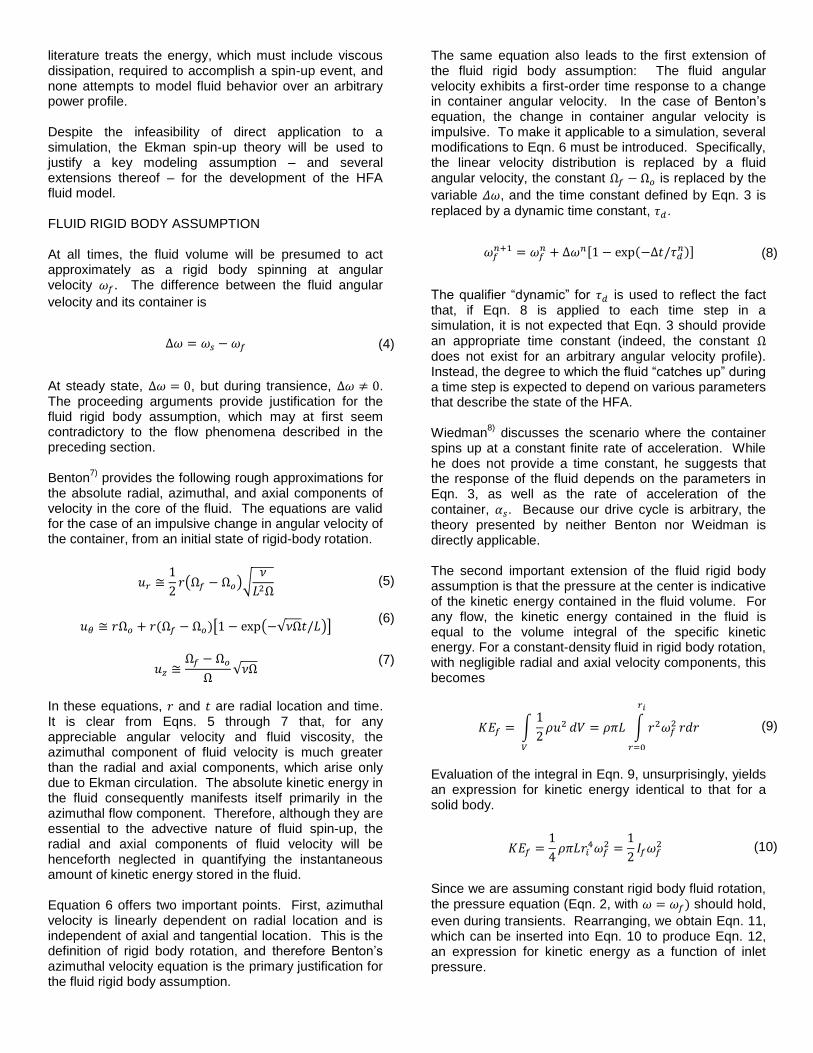
EXPERIMENTAL APPROACH The experimental apparatus must apply a transient power trace to a rotating fluid volume. During an experiment, it is necessary to measure several physical quantities is order to calculate the various parameters in Eqns. 24 and 26. Then, a curve-fitting algorithm can be used to derive an actual mathematical relationship
between the dimensionless groups. Figure 3 illustrates the experimental setup.
Figure 3: Experimental setup with instrumentation
A rotating cylinder filled with oil is driven by a hydraulic motor. Flow rate through the motor is metered using a proportioning flow control valve in a feedback control loop. In this way, the angular velocity of the rotating cylinder can be well-controlled. A rotary torque sensor and shaft encoder facilitate torque and speed measurements, and a rotary union allows for an internal pressure tap at the center of an end cap. Because the cylinder is not charged, Eqn. 2 indicates that gage pressure at the center should be negative for any nonzero rotational speed. Table 1 provides relevant specifications for some of the experimental equipment.
Table 1: Specifications for the experimental setup
Oil length,
Oil radius,
Oil density,
Oil kinematic viscosity, ( )
Maximum speed
Maximum torque
Sampling frequency
Note that angular velocity is the prescribed physical quantity for any given experiment, and therefore the applied power is, in a sense, incidental. For the purposes of characterizing viscous dissipation rate and dynamic time constant, this is perfectly acceptable, as the actual shape of the power profile is non-critical; the important point is that power can be extracted from the measured data. To confirm repeatability of measurements, the prescribed angular velocity traces are non-arbitrary. Instead, they resemble near-impulsive acceleration events. To maximize the signal to noise ratio, the angular velocity traces are rather aggressive. Figure 4 shows an example angular velocity trace used for model development, along with its equivalent ideal (step change) trace. Though not fully shown Figure 4, container angular velocity is held constant both before and after the transient for a time deemed sufficient to guarantee
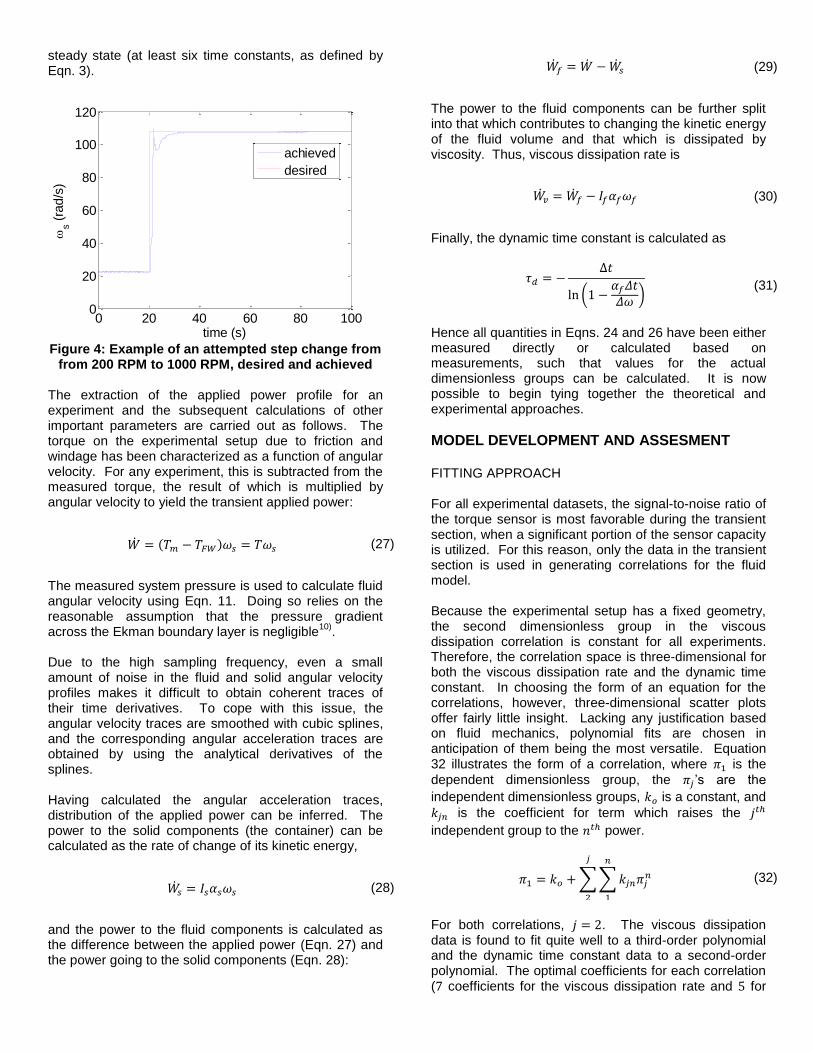
steady state (at least six time constants, as defined by Eqn. 3).
Figure 4: Example of an attempted step change from
from 200 RPM to 1000 RPM, desired and achieved The extraction of the applied power profile for an experiment and the subsequent calculations of other important parameters are carried out as follows. The torque on the experimental setup due to friction and windage has been characterized as a function of angular velocity. For any experiment, this is subtracted from the measured torque, the result of which is multiplied by angular velocity to yield the transient applied power:
(27)
The measured system pressure is used to calculate fluid angular velocity using Eqn. 11. Doing so relies on the reasonable assumption that the pressure gradient across the Ekman boundary layer is negligible
10).
Due to the high sampling frequency, even a small amount of noise in the fluid and solid angular velocity profiles makes it difficult to obtain coherent traces of their time derivatives. To cope with this issue, the angular velocity traces are smoothed with cubic splines, and the corresponding angular acceleration traces are obtained by using the analytical derivatives of the splines. Having calculated the angular acceleration traces, distribution of the applied power can be inferred. The power to the solid components (the container) can be calculated as the rate of change of its kinetic energy,
(28)
and the power to the fluid components is calculated as the difference between the applied power (Eqn. 27) and the power going to the solid components (Eqn. 28):
(29)
The power to the fluid components can be further split into that which contributes to changing the kinetic energy of the fluid volume and that which is dissipated by viscosity. Thus, viscous dissipation rate is
(30)
Finally, the dynamic time constant is calculated as
(31)
Hence all quantities in Eqns. 24 and 26 have been either measured directly or calculated based on measurements, such that values for the actual dimensionless groups can be calculated. It is now possible to begin tying together the theoretical and experimental approaches.
MODEL DEVELOPMENT AND ASSESMENT FITTING APPROACH For all experimental datasets, the signal-to-noise ratio of the torque sensor is most favorable during the transient section, when a significant portion of the sensor capacity is utilized. For this reason, only the data in the transient section is used in generating correlations for the fluid model. Because the experimental setup has a fixed geometry, the second dimensionless group in the viscous dissipation correlation is constant for all experiments. Therefore, the correlation space is three-dimensional for both the viscous dissipation rate and the dynamic time constant. In choosing the form of an equation for the correlations, however, three-dimensional scatter plots offer fairly little insight. Lacking any justification based on fluid mechanics, polynomial fits are chosen in anticipation of them being the most versatile. Equation 32 illustrates the form of a correlation, where is the
dependent dimensionless group, the ’s are the
independent dimensionless groups, is a constant, and
is the coefficient for term which raises the
independent group to the power.
(32)
For both correlations, . The viscous dissipation data is found to fit quite well to a third-order polynomial and the dynamic time constant data to a second-order polynomial. The optimal coefficients for each correlation ( coefficients for the viscous dissipation rate and for
0 20 40 60 80 1000
20
40
60
80
100
120
time (s)
s (
rad/s
)
achieved
desired

the time constant) are found by using a genetic algorithm that minimizes the sum of squared errors. Eleven experiments have been run with the desired angular velocity trace shown in Fig. 4 ( to
, near-impulsive). Each experiment yields a dataset from which both a viscous dissipation and a dynamic time constant correlation can be developed. The two correlations from each dataset can and should be assessed completely independently from one another. That is, the time constant correlation from experiment #1 is no more “related” to the viscous dissipation correlation from experiment #1 than it is to the viscous dissipation correlation from experiment #2. Therefore, the experiments yield twenty-two independent correlations, eleven candidates for the best viscous dissipation correlation and eleven candidates for the best dynamic time constant correlation. CORRELATION ASSESSMENT CRITERIA The validity of each of the correlations is assessed by applying it to each of the power profiles from the other ten experimental datasets. In other words, a correlation developed by curve-fitting data from experiment #1 can be tested by running a simulation where the power profile from experiment #2 is the input, and then comparing the resultant simulated data (viscous dissipation rate, fluid and solid angular velocity, etc.) to the measured data from experiment #2. In this way, twenty-two different correlations (eleven each for the two desired parameters) are evaluated via 220 simulations. Over the course of a simulation, the accuracy of the dynamic time constant correlation affects the indicated accuracy of the viscous dissipation correlation, and vice versa. For example, should the dynamic time constant correlation tend to under-predict the correct (measured) value, the viscous dissipation rate will consequently be under-predicted. This is intuitive, as a lower-than-realistic should result in lower-than-realistic viscous dissipation. For this reason, while the viscous dissipation correlations are being evaluated and compared, the dynamic time constant is intentionally forced to its measured value. Then, once the best viscous dissipation correlation has been identified, it is permanently embedded in the simulation code, such that its effects are included during the evaluation and comparison of the candidate dynamic time constant correlations. Quantitatively, the performance of a correlation is judged by how well it predicts container and fluid angular velocities. To produce such a judgment, the coefficient of determination, defined as
(33)
is used, where
(34)
To provide more qualitative insight into how a given correlation performs, two different coefficients of determination can be calculated:
, which includes the highly transient region
between the initial acceleration and the time at which the measured fluid angular velocity has reached 95% of its steady state value, and
, which includes the region between the initial
acceleration and the time at which the measured fluid angular velocity has reached 99% of its steady state value. This generally includes a much larger amount of near-steady state behavior
Any given correlation might perform quite differently in the highly transient section compared to the near-steady state section; examination of the two different coefficients of determination defined above provides insight into this difference. CORRELATION PERFORMANCE AND SELECTION
Table 2 shows the values of ,
, and
, for each of the eleven candidate viscous
dissipation correlations. All of these values encompass data from all ten simulations for a given correlation, such that they represent its average
performance. The correlations are ranked by .
Table 2: Ranked performance of the viscous
dissipation rate correlations, based on coefficient of determination
Corr. # Rank
7 1 0.99845 0.998825 0.998067 9 2 0.99843 0.999039 0.997830 3 3 0.99816 0.998836 0.997490 4 4 0.99805 0.998773 0.997335 1 5 0.99795 0.999171 0.996733 6 6 0.99794 0.998850 0.997036 8 7 0.99781 0.998125 0.997489 2 8 0.99685 0.998603 0.995093
11 9 0.99675 0.998599 0.994908 5 10 0.99646 0.998460 0.994452
10 11 0.99624 0.998629 0.993850
Average 0.99755 0.998719 0.996389 Standard Dev. 0.00081 0.000284 0.001511
On average a viscous dissipation correlation predicts the
container and fluid angular velocities with at
. Quantitatively, there is relatively little difference in how well the correlations behave through 95% of steady state. Including data through 99% causes in increase in total squared error for all correlations and reveals more
variation amongst them, increasing standard deviation by an order of magnitude. In other words, there is a wider range of performance amongst the correlations for steady state, but each performs worse at steady state than it does during transience.
Because it produces the highest value of ,
viscous dissipation correlation #7 is selected for use in the fluid model. As indicated in Table 2, this correlation performs better than all but two in transience, and better than any other when data through 99% of steady state is included. The full expression for the selected viscous dissipation correlation is:
(35)
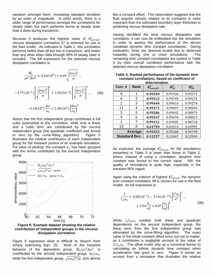
Notice that the first independent group contributes a full cubic polynomial to the correlation, while only a linear and a cubic term are contributed by the second independent group (the quadratic coefficient was forced to zero by the curve-fitting algorithm). Figure 5 illustrates the relative contribution of each independent group for the transient portion of an example simulation. For ease of plotting, the constant has been grouped with the terms contributed by the second independent group.
Figure 5: Example dataset showing the relative
contribution of independent groups in the viscous dissipation correlation
Figure 5 expresses what is difficult to discern from simply examining Eqn. 35. Most of the transient
behavior of the dependent group,
, is
contributed by the second independent group, ,
while the first independent group, , acts almost
like a constant offset. This observation suggests that the fluid angular velocity relative to its container is more important than the estimated boundary layer thickness in predicting viscous dissipation rate. Having identified the best viscous dissipation rate correlation, it can now be embedded into the simulation in order to assess the performance of the eleven candidate dynamic time constant correlations. During evaluation, three are deemed invalid due to observed instability during one or more simulations. The remaining time constant correlations are ranked in Table 3 by their overall combined performance with the selected viscous dissipation correlation.
Table 3: Ranked performance of the dynamic time constant correlations, based on coefficient of
determination
Corr. # Rank
8 1 0.99549 0.99726 0.99371
6 2 0.99513 0.99749 0.99276
2 3 0.99444 0.99614 0.99274
11 4 0.99371 0.99697 0.99045
5 5 0.99286 0.99692 0.98879
9 6 0.99247 0.99670 0.98823
1 7 0.99151 0.99585 0.98718
10 8 0.64704 0.64414 0.64995
Average 0.95033 0.95268 0.94798
Standard Dev. 0.12257 0.12467 0.12044
As expected, the average for the simulations
presented in Table 3 is lower than those in Table 2, where, instead of using a correlation, dynamic time constant was forced to the correct value. Still, the quality of simulations is quite high, especially in the transient 95% region.
Again using the criterion of highest , the dynamic
time constant correlation #8 is chosen for use in the fluid model. Its full expression is:
(36)
While exhibits both linear and quadratic dependence on the second independent group, the linear term from the first independent group was eliminated by the curve-fitting algorithm. The exact value of the small constant offset turns out not to matter, as it contributes a negligible amount to the value of . The offset exists only as a numerical barrier to calculating an infinite dynamic time constant when acceleration rate goes to zero. Figure 6 shows an excerpt from a simulation that illustrates the relative
60 62 64 66 68 70 720
1000
2000
3000
4000
5000
time (s)
dim
ensio
nle
ss v
alu
e

importance of the two independent groups in the dynamic time constant correlation.
Figure 6: Example dataset showing the relative
contribution of terms in the dynamic time constant correlation
As was the case for the viscous dissipation correlation, the relative contribution from the two independent variables is rather lopsided. The dependent variable response is dictated mostly by the behavior of the term
and corrected only slightly by the term .
It is worth noting that, as steady state is approached, error in the predicted dynamic time constant becomes simultaneously greater in value and less important in effect. The former is true because the time constant is inversely proportional to the container acceleration and therefore sensitive to error as acceleration goes to zero. The latter is true because, as steady state is approached, shrinks, and therefore any error in the predicted time constant is multiplied by a smaller value in the calculation of the fluid velocity for the subsequent time step. FLUID MODEL ASSESSMENT The predictive model whose development has been detailed in the preceding sections can be executed with only a few lines of code. Simulations were run using MATLAB
® on a modest processor. Even without any
attempt to maximize computational efficiency, a three minute simulation with one millisecond temporal resolution can be completed in approximately one second. In this regard, the requirement that the model be computationally inexpensive has been overwhelmingly achieved. Before presenting the model performance, a certain unanticipated nuance in the measured fluid behavior is described. In experiments with significant overshoot and rapid recovery of container angular velocity, a negative time constant can be observed for a small period of time. An example is illustrated in Fig. 7, where the fluid angular velocity can be seen to follow a qualitatively similar profile as the container angular velocity, spiking
and beginning to decrease, even though never ceases to be positive.
Figure 7: Example of a region with an observed
negative time constant To the authors’ knowledge, there is no physical explanation for the region of observed negative time constant shown in Fig. 7; the fluid angular velocity should increase as long as it remains below the container angular velocity. It is therefore postulated that, during strong acceleration, flow phenomena in the Ekman boundary layer generate a pressure gradient that causes the pressure sensor to read somewhat lower (more vacuum) than the true value in the fluid core. This is translated via Eqn. 11 to a somewhat over-predicted fluid angular velocity. A sudden deceleration of the container is accompanied by a reversal in the aforementioned flow phenomena, the net result of which is to generate a fluid angular velocity trace which exhibits some non-physical behavior. It must be noted that characterizing a dynamic time constant is extremely useful, regardless of how well the measured pressure indicates fluid angular velocity. The ability to predict the transient response of pressure itself is essential in developing a control strategy that effectively regulates hydraulic system pressure. The detrimental effect of the behavior shown in Fig. 7, then, is to overestimate (in positive acceleration) the rate of change of fluid kinetic energy, thereby introducing some error into the energy equation (Eqn. 15). For the purposes of assessing model performance, the remainder of the discussion relies on the assumption that the calculated fluid angular velocity is reasonably accurate. In addition the requirement of computational simplicity, the fluid model must realistically predict HFA behavior. As a general illustration of the performance of the model, Figures 8, 9 and 10 show angular velocities, dynamic time constant, and viscous dissipation rate, respectively, for the transient portion of an example simulation. The plots show simulated quantities and their corresponding measured quantities. This example comes from a dataset that, importantly, is not the same one that
60 60.5 61 61.5 62-0.1
0
0.1
0.2
0.3
0.4
0.5
0.6
time (s)
dim
ensio
nle
ss v
alu
e
60 61 62 63 6460
70
80
90
100
110
time (s)
angula
r velo
city (
rad/s
)
container
fluid
generated either of the correlations chosen for the fluid
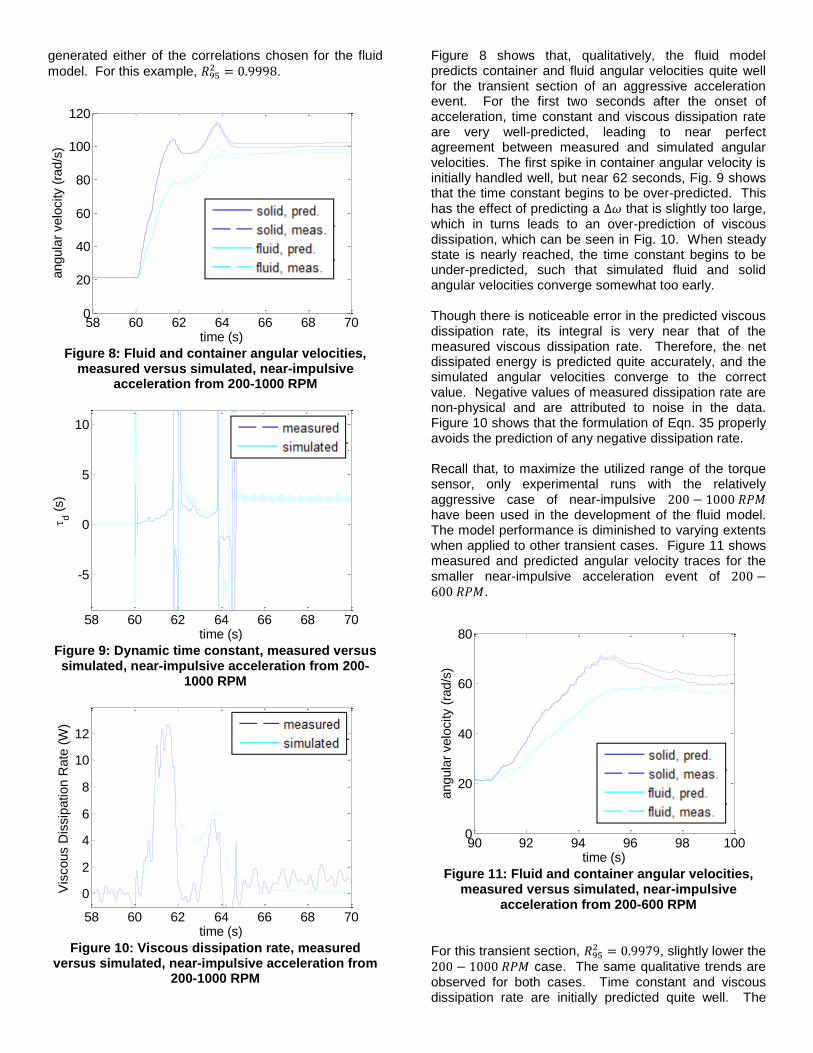
model. For this example, .
Figure 8: Fluid and container angular velocities,
measured versus simulated, near-impulsive acceleration from 200-1000 RPM
Figure 9: Dynamic time constant, measured versus simulated, near-impulsive acceleration from 200-
1000 RPM
Figure 10: Viscous dissipation rate, measured
versus simulated, near-impulsive acceleration from 200-1000 RPM
Figure 8 shows that, qualitatively, the fluid model predicts container and fluid angular velocities quite well for the transient section of an aggressive acceleration event. For the first two seconds after the onset of acceleration, time constant and viscous dissipation rate are very well-predicted, leading to near perfect agreement between measured and simulated angular velocities. The first spike in container angular velocity is initially handled well, but near 62 seconds, Fig. 9 shows that the time constant begins to be over-predicted. This has the effect of predicting a that is slightly too large, which in turns leads to an over-prediction of viscous dissipation, which can be seen in Fig. 10. When steady state is nearly reached, the time constant begins to be under-predicted, such that simulated fluid and solid angular velocities converge somewhat too early. Though there is noticeable error in the predicted viscous dissipation rate, its integral is very near that of the measured viscous dissipation rate. Therefore, the net dissipated energy is predicted quite accurately, and the simulated angular velocities converge to the correct value. Negative values of measured dissipation rate are non-physical and are attributed to noise in the data. Figure 10 shows that the formulation of Eqn. 35 properly avoids the prediction of any negative dissipation rate. Recall that, to maximize the utilized range of the torque sensor, only experimental runs with the relatively aggressive case of near-impulsive have been used in the development of the fluid model. The model performance is diminished to varying extents when applied to other transient cases. Figure 11 shows measured and predicted angular velocity traces for the smaller near-impulsive acceleration event of .
Figure 11: Fluid and container angular velocities,
measured versus simulated, near-impulsive acceleration from 200-600 RPM
For this transient section, , slightly lower the
case. The same qualitative trends are observed for both cases. Time constant and viscous dissipation rate are initially predicted quite well. The
58 60 62 64 66 68 700
20
40
60
80
100
120
time (s)
angula
r velo
city (
rad/s
)
solid, pred.
solid, meas.
fluid, pred.
fluid, meas.
58 60 62 64 66 68 70
-5
0
5
10
time (s)
d (
s)
measured
simulated
58 60 62 64 66 68 70
0
2
4
6
8
10
12
time (s)
Vis
cous D
issip
ation R
ate
(W
)
measured
simulated
90 92 94 96 98 1000
20
40
60
80
time (s)
angula
r velo
city (
rad/s
)
solid, pred.
solid, meas.
fluid, pred.
fluid, meas.

spike in container angular velocity has a small detrimental effect on the latter, causing the simulated angular velocities to reach steady state too soon. A slight over-prediction in net dissipated energy causes the final simulated angular velocity to be a few radians per second lower than the measured value. In full, the model proves to be fairly robust for the near-impulsive case. The model performance suffers much more when the initial angular velocity is different than that which was used to produce the correlations. Figure 12 shows the case of near-impulsive acceleration from .
Figure 12: Fluid and container angular velocities,
measured versus simulated, near-impulsive acceleration from 600-1000 RPM
In this case, , which is significantly lower
than either of the previously presented cases. The model substantially over-predicts the dynamic time constant from the beginning of the transient. While predicted container angular velocity is initially quite accurate, the artificially large generates an erroneously high simulated rate of viscous diffusion. This drags the predicted steady state angular velocity down to a value significantly below the correct value. As a final example of the versatility of the fluid model, it is useful to examine the case of a non-impulsive acceleration. Figure 13 shows the predicted and measured angular velocities for the case of a mild acceleration from over the course of
about seconds. Compared to the near-impulsive
example illustrated in Figures 8 through 10, the average acceleration for this milder case is lower by a factor of three, and the maximum observed rate of acceleration is lower by a factor of ten. Qualitatively, the model performance for this transient section falls somewhere between the two shorter, near-impulsive cases shown in Figures 11 and 12. Here, however, the viscous dissipation rate is the more error-prone correlation. The measured viscous dissipation rate is so close to zero that the model tends to over-
predict it. The result of this it under-predict both angular velocities, even though the time constant is reasonably accurate.
Figure 13: Fluid and container angular velocities, measured versus simulated, gradual acceleration
from 100-800 RPM
CONCLUSION This paper detailed the theory and experiments used to develop a model for the transient behavior of a rotating fluid volume. The model relies on the assumption that, under applied power, the fluid volume accelerates roughly as a rigid body and lags behind its container in a manner that can be modeled as a first-order time response. The simplicity of the model allows it to simulate the transient HFA performance orders of magnitude more quickly than would be possible if CFD were used. This makes it quite applicable to a highly-resolved drive cycle simulation nested within a comprehensive design optimization. The fluid model relies on correlating dimensionless groups of relevant parameters for viscous dissipation rate and dynamic time constant. The structure of these two correlations was chosen to be, respectively, a third- and second-order polynomial, excluding binomial terms. A genetic algorithm was used to find the set of
polynomial coefficients that produced the smallest value when fit to experimental data. By comparing simulations to measured data, the fluid model was shown to perform well for transient sections of intense acceleration and large . To varying degrees, the performance of the model was observed to decrease when applied to other types of transients. For intense accelerations in general, the model predicts viscous dissipation rate quite well. However, when the initial angular velocity is very far from that used to develop the correlation ( ), prediction of the dynamic time constant is notably hindered. Conversely, for cases where acceleration is milder, time constant is accurately predicted, while viscous dissipation rate tends to be over-predicted. To improve the robustness of the
60 62 64 66 68 7050
60
70
80
90
100
110
120
130
time (s)
angula
r velo
city (
rad/s
)
solid, pred.
solid, meas.
fluid, pred.
fluid, meas.
60 65 70 75 800
20
40
60
80
100
time (s)
angula
r velo
city (
rad/s
)
solid, pred.
solid, meas.
fluid, pred.
fluid, meas.

model, experimental data representing a wider variety of transients will be used in future work. During experimental data collection, pressure was measured at at the face of one of the container end caps. There is some uncertainty as to how well this pressure measurement indicates the true pressure in the fluid core. Future work will deal with this uncertainty by either modifying the experimental apparatus to measure pressure away from the end cap, or by attempting to characterize the pressure gradient across the boundary layer that might arise from Ekman flow phenomena. Finally, it is important to note that the model developed and assessed in this paper is specific to the experimental setup used to create it. Container aspect ratio, which was included as an independent group in the dimensional analysis, was not varied in the experiments, and was therefore not correlated. To make the model fully applicable to a design optimization, all relevant dimensionless groups must be correlated. Future work will include the ability to vary the geometry of the container and/or the fluid properties used in the experiments. Then, the experimental methods and computational tools described in this paper can be used to explore the full dimensionless space that characterizes the transient response of a rotating fluid to an arbitrary power profile.
ACKNOWLEDGMENTS
This work was sponsored by the National Science Foundation through the Center for Compact and Efficient Fluid Power, grant EEC-0540834.
REFERENCES
1) Pourmovahed, A., “Sizing Energy Storage Units for
Hydraulic Hybrid Vehicle Applications,” ASME
Dynamic Systems and Controls Div., New York, NY,
1993, 52, pp. 231-246
2) Sclater, N., “Electronic Technology Handbook,”
McGraw-Hill, New York, NY, 1999
3) Van de Ven, J.D., “Increasing Hydraulic Energy
Storage Capacity: Flywheel-Accumulator,”
International Journal of Fluid Power, Vol. 10, No. 3,
2009, pp. 41-50
4) Pourmovahed, A., Baum, S.A., Fronczak, F.J., and
Beachley, N.H., “Experimental Evaluation of
Hydraulic Accumulator Efficiency With and Without
Elastomeric Foam,” Journal of Propulsion and
Power, Vol. 4, No. 2, 1988, pp. 185-192
5) Strohmaier, K.G. and Van de Ven, J.D., “Constrained
Multi-Objective Optimization of a Hydraulic Flywheel
Accumulator,” ASME/Bath Symposium on Fluid
Power and Motion Control, 2013
6) Greenspan, H.P. and Howard, L.N., “On a time-
dependent motion of a rotating fluid,” Journal of
Fluid Mechanics, Vol. 17, No. 3, 1963, pp. 385-404
7) Benton, E.R. and Clark Jr., A., “Spin-up,” Annual
Review of Fluid Mechanics, Vol.6, No. 1, 1974, pp.
257-280
8) Wiedman, P.D., “On the spin-up and spin-down of a
rotating fluid. Part 1. Extending the Wedemeyer
model,” Journal of Fluid Mechanics, Vol. 77, No. 4,
1976, pp. 685-708
9) Duck, P.W. and Foster, M.R., “Spin-up of
homogeneous and stratified fluids,” Annual Review
of Fluid Mechanics, Vol. 33, No. 1, 2001, pp. 231-
263
10) Wedemeyer, E.H., “The unsteady flow within a
spinning cylinder,” Journal of Fluid Mechanics, Vo.
20, No. 3, 1964, pp. 383-399
CONTACT
Kyle G. Strohmaier M.S.M.E. candidate Department of Mechanical Engineering University of Minnesota [email protected] James D. Van de Ven, PhD Assistant Professor Department of Mechanical Engineering University of Minnesota [email protected]