Embed Size (px)
Citation preview
Experimental Investigation of Nonlinear Mode Shape in
Microscale Beams
An Undergraduate Honor Thesis
Presented in Partial Fulfillment of the Requirements for Graduation with Distinction
Mechanical Engineering at The Ohio State University
By
Min Ma
The Ohio State University
Spring, 2017
Committee: Dr. Hanna Cho; Dr. Jason Dreyer

Copyright by
Min Ma
Spring 2017
i
Abstract
Micro-electro-mechanical-systems (MEMS) have drawn a great interest over last serval decades due
to its wide applications including accelerometers and pressure sensors, micro-mirrors, radiofrequency
(RF) switches, microphones, and inertia sensors. The moving mechanical element integrated in MEMS
devices is typically operating in its resonant mode. Due to its small size and low damping, the micro-
beams often exhibit the nonlinear resonance, which is being widely investigated to overcome the
limitations of linear mode in term of its levels of sensitivity and reliability. This work covers an
experimental study of the dynamic responses of micro-beams, including the nonlinear mode shape and
resonances by improving the experimental tool and accuracy. The characterization is performed on a
silicon-polymer micro-beam that is excited near its fundamental mode frequency by a piezoelectric
shaker. The nonlinearity of this micro-beam originates geometrically from the elongation of the
polymer part during large flexural oscillations of the silicon part. Its amplitude of oscillation is detected
by Laser Doppler Vibrometer (LDV) while the excitation frequency is varied. To study the nonlinear
mode shape, the points of measurement are scanned along the longitudinal direction of the micro-beam
located on a 2-axis piezoelectric stage. A custom LabVIEW program which can precisely control the
movable stage and collect the vibration amplitude data at different locations was developed. The
experimental measurement provides the most realistic mode shape of the micro-beam and gives a
better understanding of the vibration behavior of MEMS resonators.

ii
Acknowledgments
First and foremost, I would like to thank my research advisor, Professor Hanna Cho. Without her
guidance and dedicated involvement in every step throughout the process, this paper would have never
been accomplished. I would like to thank her very much for her support and understanding over the past
year on this project.
I greatly appreciate Mr. Keivan Asadi’s help. He has being so generous with his time in processing
partial experiment data and explaining to me. I also would to like to thank for Dr. Hatem Brahmi for
his time revising my thesis and fundamental explanation of this research.
iii
Vita
June, 1991 --------------------------------------------------------------------------------------- Changzhi, China
2010 to 2012 -------------------------------------------------------------------------- Xiamen University, China
2013 to 2014 ------------------------------------------------------------------- Arizona State University, U.S.A
2014 to 2017 ---------------------------------------------------------------------- Ohio State University, U.S.A
Fields of Study
Major Field: Mechanical Engineering
iv
Table of Contents
Abstract ................................................................................................................................................... i
Acknowledgments.................................................................................................................................. ii
Vita ....................................................................................................................................................... iii
List of Figures ........................................................................................................................................ v
List of Tables ......................................................................................................................................... vi
Chapter 1: Introduction .......................................................................................................................... 1
1.1 Motivation .................................................................................................................................... 1
1.2 Objective ...................................................................................................................................... 5
Chapter 2: Fundamental Background .................................................................................................... 6
2.1 Linear Vibration ........................................................................................................................... 6
2.2 Nonlinear Vibration.................................................................................................................... 12
Chapter 3. Experiment Setup and Measurements ................................................................................ 15
3.1 Experimental setup..................................................................................................................... 15
3.2 Measurement Procedure............................................................................................................. 19
Chapter 4. Results and Discussion……………………………………………………………………25 4.1 LabVIEW Programs ................................................................................................................... 23
4.2. Experimental results and processed data: ................................................................................. 30
Chapter 5: Conclusion and Future works............................................................................................. 41
Appendix: ............................................................................................................................................. 42
Custom LabVIEW part 1 ................................................................................................................. 43
Custom LabVIEW part 2 ................................................................................................................. 44
MATLAB code..................................................................................................................................... 45
Reference ............................................................................................. Error! Bookmark not defined.
v
List of Figures Figure 1: Challenge of MEMS ............................................................................................................... 3 Figure 2: Spring-Mass-Damper System................................................................................................. 6 Figure 3: Bode plot for different zeta values ......................................................................................... 8 Figure 4: Linear mode shapes of cantilever beam and corresponding frequency response ................... 9 Figure 5: Linear mode shape (1st, 2nd and 3rd modes) of a fixed-fixed beam ................................... 10 Figure 6: Free body diagram of a section of beam under transverse vibration .................................... 10 Figure 7: Mode shape of Cantilever beam ........................................................................................... 12 Figure 8: SDOF spring-mass- damper system with nonlinear stiffness .............................................. 13 Figure 9: Linear and Nonlinear response ............................................................................................. 14 Figure 10:Sechmatic experimental setup ............................................................................................. 15 Figure 11: Experimental setup ............................................................................................................. 16 Figure 12: Piezoelectric stage .............................................................................................................. 17 Figure 13: Logic Statement of moving piezoelectric stage ................................................................. 18 Figure 14: Schematic image of the silicon beam microstructure ......................................................... 19 Figure 15: SEM image of the silicon beam/polymer microstructure ................................................... 19 Figure 16: User interface panel and LabVIEW program diagram for the thermal frequency measurement ........................................................................................................................................ 21 Figure 17: User Panel for the main LabVIEW program ...................................................................... 23 Figure 18: E873_Configuration_Setup.vi ............................................................................................ 25 Figure 19: Switch Servo on program’s diagram .................................................................................. 26 Figure 20: FRF and FRF? Program’s diagram ..................................................................................... 27 Figure 21: MOV and ONT? Program .................................................................................................. 28 Figure 22: MVR and POS? .................................................................................................................. 29 Figure 23: Thermal Frequency response showing the 3 first natural frequencies of silicon micro cantilever .............................................................................................................................................. 30 Figure 24: Frequency response of cantilever for first mode ................................................................ 31 Figure 25: First mode shape of micro cantilever beam........................................................................ 32 Figure 26: Second model shape of micro cantilever beam .................................................................. 32 Figure 27: Third model shape of micro cantilever beam ..................................................................... 33 Figure 28 Normalized first mode shape of micro cantilever ............................................................... 34 Figure 29: Normalized third mode shape of micro cantilever ............................................................. 35 Figure 30 Normalized second mode shape of micro cantilever ........................................................... 35 Figure 31 Thermal Frequency response showing the three first natural frequencies of polymer/silicon micro beam structure............................................................................................................................ 36 Figure 32: First mode shape of the fixed-fixed micro beam ................................................................ 38 Figure 33: Third mode shape of the fixed-fixed micro beam .............................................................. 39
vi
List of Tables Table 1 E873_Configuration_Setup value ........................................................................................... 25 Table 2 SVO settings ........................................................................................................................... 26 Table 3 SVO? settings .......................................................................................................................... 26 Table 4 FRF settings ............................................................................................................................ 27 Table 5 FRF? settings ........................................................................................................................... 27 Table 6 MOV settings .......................................................................................................................... 28 Table 7 ONT? Settings ......................................................................................................................... 28 Table 8: MVR settings ......................................................................................................................... 29 Table 9 Natural frequencies of the micro cantilever beam .................................................................. 37 Table 10 Silicon Material Properties .................................................................................................... 37 Table 11 Theoretical coefficient value of c .......................................................................................... 40 Table 12 Natural frequencies of the fixed-fixed micro beam .............................................................. 40 Table 13 measurement data .................................................................................................................. 30 Table 14 coefficient of first mode shape of fixed-fixed beam ............................................................. 33 Table 15 coefficient of second mode shape of fixed-fixed beam ........................................................ 34
1
Chapter 1: Introduction
1.1 Motivation
Several decades have passed by since the discovery and development of micro-electro-
mechanical-systems (MEMS). This technology has reached a level of maturity that delivers
commodity products for our everyday life, such as integrated multi-sensor modules (9 degrees-of-
freedom inertial, gas, pressure, temperature, and flow), actuators (inkjet nozzles, digital mirror
displays), communication components (RF filters, oscillators, duplexers), and other transducers
(power harvesters). Nowadays, hundreds of foundries around the world offer numerous fabrication
services that can translate the imagination of a MEMS designer of a device into reality. Even with the
development of fabrication processes and commercialization, MEMS are still one of the hottest
evolving areas in science and engineering. Scientists from across various disciplines investigate,
brainstorm, and collaborate to invent smarter devices, develop new technologies, and innovate unique
solutions. The forecasts for the MEMS market shows a compound annual growth rate of 5–24% for
the period 2013–2019 [1]. The increasing impact that MEMS have on markets is caused by their
typically small size, which makes them minimally invasive into larger systems.
The easiest way to introduce MEMS is referring to the acronym MEMS itself. MEMS stands for
micro-electro-mechanical-systems. Hence, they are devices in the “micro” scale, in which one or more
of their dimensions are in the micrometer range. The “electro” part indicates that they use electric
signals and power. “Mechanical” means these devices rely on some sort of mechanical motion, action,
or mechanism. The word “system” refers to the fact that they function as integrated systems and not

2
as individual components. Thereby, MEMS are attributed to the integration of mechanical elements,
sensors, actuators, and electronics on a common silicon substrate through micro-fabrication technology.
MEMS technology covers different fields including sensors, actuators, RF-MEMS, Optical-
MEMS, Microfluidic-MEMS, and Bio-MEMS [2]. So far the sensor industry is the most-developed
and productive sector for MEMS and shows top-notch technology with high efficiency and long life
performance. Examples of MEMS sensor areas include pressure sensors, accelerometers, gas and mass
sensors, temperature sensors, force sensors, and humidity sensors. Historically speaking, the early
generation of MEMS researchers has relied on journals and conferences of sensors and actuators to
disseminate their research on miniature devices before the introduction of specialized MEMS
conferences and journals in the early 1990s.
The fascination in the MEMS technology comes from their distinguished characteristics. MEMS
are characterized by low cost which is a direct consequence of the batch fabrication. This means that
each fabrication batch can produce thousands of MEMS devices all at once. They are lightweight and
small which is desirable for compactness and convenience reasons. The fabrication of MEMS devices
usually starts with single crystal silicon wafers which come in many standard sizes. Silicon is the ideal
material due to its excellent thermal and mechanical properties [2] (stable mechanism, high melting
point, high toughness, and smallest thermal expansion coefficient). In addition, their small size allows
the implementation of MEMS in tight locations where large devices do not fit, such as engines in cars
[3] and inside the human body [4]. Moreover, they consume very low power which not only reduces
the operational cost but also enables the development of long-life and self-powered devices that can
3
harvest a small amount of energy they need from the environment during their operation. Furthermore,
MEMS devices have enabled many superior performances, smart functionalities, and complicated
tasks that cannot be achieved in other technologies. For proof of their uniqueness one can cite examples
of ultra-sensitive mass detectors [5], high isolation and low-insertion-loss RF switches [6], lab-on-a-
chip bio-sensors [6], tiny directional microphones for hearing aids [6], high-temperature pressure
sensors for automobile engines [6], and precise controlled liquid droplets for ink-jet printers [6].
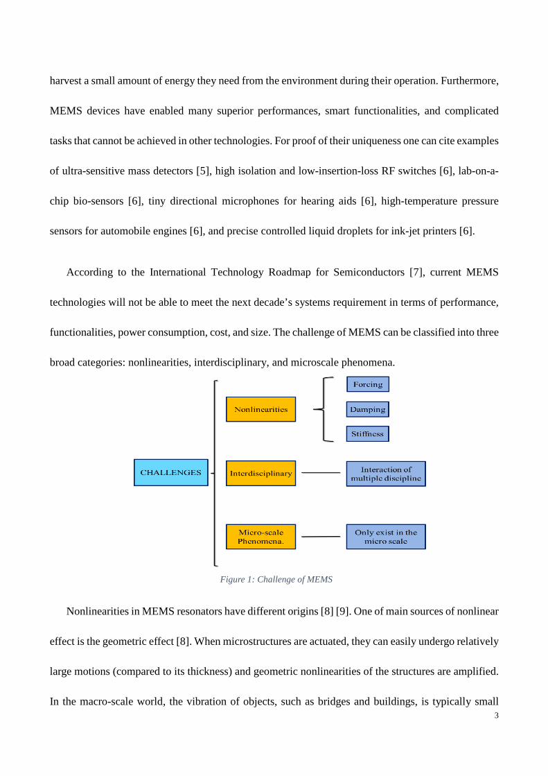
According to the International Technology Roadmap for Semiconductors [7], current MEMS
technologies will not be able to meet the next decade’s systems requirement in terms of performance,
functionalities, power consumption, cost, and size. The challenge of MEMS can be classified into three
broad categories: nonlinearities, interdisciplinary, and microscale phenomena.
Nonlinearities in MEMS resonators have different origins [8] [9]. One of main sources of nonlinear
effect is the geometric effect [8]. When microstructures are actuated, they can easily undergo relatively
large motions (compared to its thickness) and geometric nonlinearities of the structures are amplified.
In the macro-scale world, the vibration of objects, such as bridges and buildings, is typically small
Figure 1: Challenge of MEMS
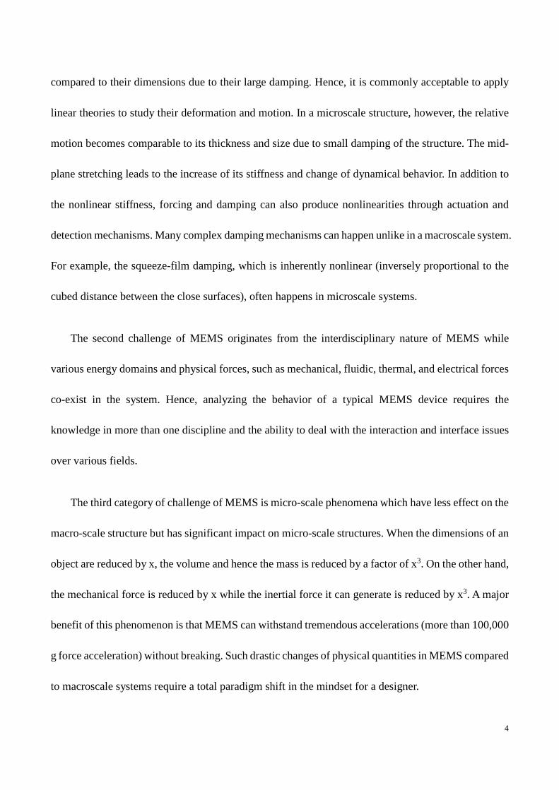
4
compared to their dimensions due to their large damping. Hence, it is commonly acceptable to apply
linear theories to study their deformation and motion. In a microscale structure, however, the relative
motion becomes comparable to its thickness and size due to small damping of the structure. The mid-
plane stretching leads to the increase of its stiffness and change of dynamical behavior. In addition to
the nonlinear stiffness, forcing and damping can also produce nonlinearities through actuation and
detection mechanisms. Many complex damping mechanisms can happen unlike in a macroscale system.
For example, the squeeze-film damping, which is inherently nonlinear (inversely proportional to the
cubed distance between the close surfaces), often happens in microscale systems.
The second challenge of MEMS originates from the interdisciplinary nature of MEMS while
various energy domains and physical forces, such as mechanical, fluidic, thermal, and electrical forces
co-exist in the system. Hence, analyzing the behavior of a typical MEMS device requires the
knowledge in more than one discipline and the ability to deal with the interaction and interface issues
over various fields.
The third category of challenge of MEMS is micro-scale phenomena which have less effect on the
macro-scale structure but has significant impact on micro-scale structures. When the dimensions of an
object are reduced by x, the volume and hence the mass is reduced by a factor of x3. On the other hand,
the mechanical force is reduced by x while the inertial force it can generate is reduced by x3. A major
benefit of this phenomenon is that MEMS can withstand tremendous accelerations (more than 100,000
g force acceleration) without breaking. Such drastic changes of physical quantities in MEMS compared
to macroscale systems require a total paradigm shift in the mindset for a designer.

5
Many researchers and engineers focus on the mechanical behavior of MEMS devices and their
statics and dynamics behavior to improve the performance of MEMS. In this work, we focus on
understanding nonlinear behavior of MEMS devices induced by the geometric originations. The linear
dynamics of microstructure, such as micro beam or microcantilever, are successfully predicted by
Euler-Bernoulli theory [9]. Even though the nonlinear resonance has been widely investigated in both
theoretical and experimental ways, the nonlinear mode shape of various mirco-resonators has not been
studied rigorously.
1.2 Objective
The first purpose of this research is to characterize the dynamic behavior of two type micro-beams
by experimentally capturing their nonlinear mode shape. To do so, measurement of the vibration
amplitude was performed at multiple scan points using Laser Dropper Vibrometer. Then the collected
data was processed and analyzed in MATLAB to extract the vibration mode shape.
The second purpose of this research is to improve the current measurement setup. To achieve this
goal, the capability of an existing experimental setup was enhanced by integrating an automated scan
of different locations of the vibrating micro-beams. Using a piezoelectric linear stage, an accurate scan
step as small as 4 nm was achieved. All the measurement equipment was controlled through one main
LabVIEW program.
6
Chapter 2: Fundamental Background
2.1 Linear Vibration
2.1.1 Dynamics of single degree of freedom systems
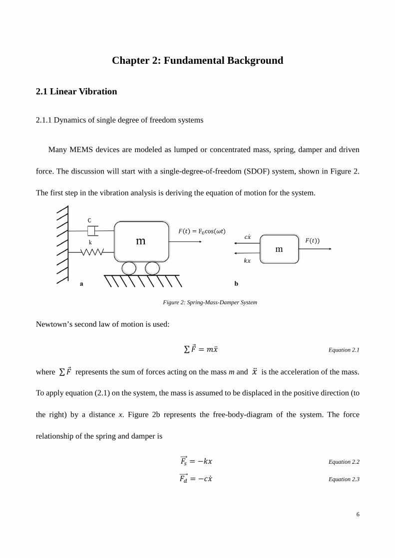
Many MEMS devices are modeled as lumped or concentrated mass, spring, damper and driven
force. The discussion will start with a single-degree-of-freedom (SDOF) system, shown in Figure 2.
The first step in the vibration analysis is deriving the equation of motion for the system.
Newtown’s second law of motion is used:
∑ �⃗�𝐹 = 𝑚𝑚�̈�𝑥 Equation 2.1
where ∑ �⃗�𝐹 represents the sum of forces acting on the mass m and �̈�𝑥 is the acceleration of the mass.
To apply equation (2.1) on the system, the mass is assumed to be displaced in the positive direction (to
the right) by a distance x. Figure 2b represents the free-body-diagram of the system. The force
relationship of the spring and damper is
𝐹𝐹𝑠𝑠���⃗ = −𝑘𝑘𝑥𝑥 Equation 2.2
𝐹𝐹𝑑𝑑����⃗ = −𝑐𝑐�̇�𝑥 Equation 2.3
Figure 2: Spring-Mass-Damper System
7
where k is the spring stiffness, c is the damping coefficient, and the negative sign indicates that the
force is in the opposite direction of motion. The systems are driven by a harmonic force excitation
given by
𝐹𝐹(𝑡𝑡) = 𝐹𝐹𝑜𝑜𝑐𝑐𝑐𝑐𝑐𝑐 (𝜔𝜔𝑡𝑡) Equation 2.4
where 𝐹𝐹𝑜𝑜 is the harmonic force amplitude and 𝜔𝜔 is the excitation frequency. Appling Eqs. 2.2-2.4,
we get the second order, linear ordinary differential equation governing the displacement of the SDOF
system:
𝑚𝑚�̈�𝑥 + 𝑐𝑐�̇�𝑥 + 𝑘𝑘𝑥𝑥 = 𝐹𝐹𝑜𝑜𝑐𝑐𝑐𝑐 𝑐𝑐(𝜔𝜔𝑡𝑡). Equation 2.5
Dividing Equation 2.5 by m yields
�̈�𝑥 + 2𝜉𝜉𝜔𝜔𝑛𝑛�̇�𝑥 + 𝜔𝜔𝑛𝑛2𝑥𝑥 =𝑓𝑓𝑜𝑜𝑐𝑐𝑐𝑐𝑐𝑐 (𝜔𝜔𝑡𝑡) Equation 2.6
where 𝑓𝑓𝑜𝑜 = 𝐹𝐹0𝑚𝑚
, and 𝜉𝜉 is the damping ratio, a nondimensional quantity described by
𝜉𝜉 = 𝑐𝑐2𝑚𝑚𝜔𝜔𝑛𝑛
Equation 2.7
where 𝜔𝜔𝑛𝑛 is called underdamped natural frequency in rad/sec, defined as:
𝜔𝜔𝑛𝑛 = �𝑘𝑘 𝑚𝑚� Equation 2.8
The steady state response of this system can be written as:
𝑥𝑥(𝑡𝑡) = 𝐴𝐴 𝑐𝑐𝑐𝑐𝑐𝑐(𝜔𝜔𝑡𝑡) + 𝐵𝐵𝑐𝑐𝐵𝐵𝐵𝐵 (𝜔𝜔𝑡𝑡) Equation 2.9
A more convenient way to express this solution is:
𝑥𝑥(𝑡𝑡) = 𝐴𝐴𝑐𝑐𝑐𝑐𝑐𝑐 (𝜔𝜔𝑡𝑡 − 𝜃𝜃) Equation 2.10
8
where
𝐴𝐴 = 𝑓𝑓0
��𝜔𝜔𝑛𝑛2−𝜔𝜔2�2+(2𝜉𝜉𝜔𝜔𝑛𝑛𝜔𝜔)2
Equation 2.11
𝜃𝜃 = 𝑡𝑡𝑡𝑡𝐵𝐵−1(2𝜉𝜉𝜔𝜔𝑛𝑛𝜔𝜔𝜔𝜔𝑛𝑛2−𝜔𝜔2) Equation 2.12
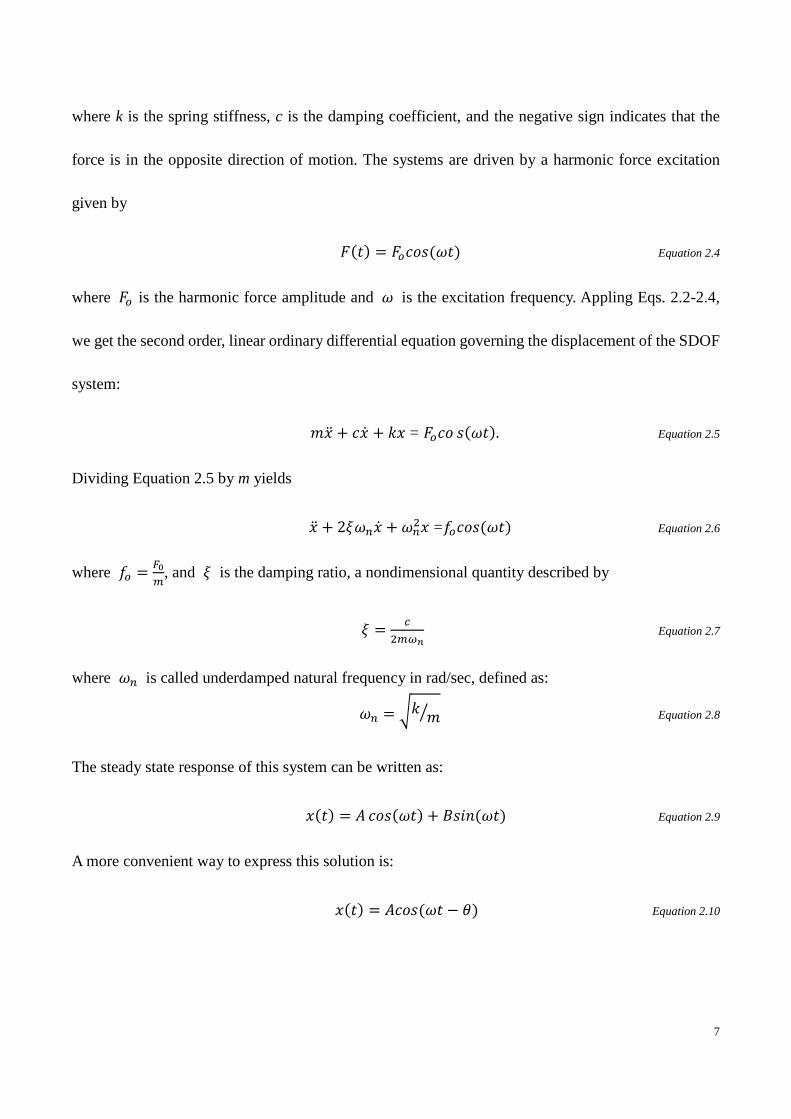
Figure 3 shows the amplitude A and phase angle 𝜃𝜃 of the spring-mass-damper system when the
input frequency is varied. The frequency response of a small ξ (smaller than 0.707) has a peak near
𝜔𝜔 = 𝜔𝜔𝑛𝑛, called resonance phenomenon. When the excitation frequency is equal or near to the natural
frequency, the system with low damping oscillates at a large amplitude. A system with ξ larger than
0.707 does not have any peak, i.e., no resonance occurs. Most MEMS resonators exhibit this resonance
behavior owing to the lower values of damping ratio. In MEMS, quality factor Q is more commonly
used to characterize the system’s damping, defined as:
𝑄𝑄 = 12𝜉𝜉
Equation 2.13
Figure 3: Bode plot for different zeta values
9
Q factor describes how an under-damped oscillator or resonator is and characterizes a resonator's
bandwidth relative to its center frequency. Higher Q indicates a lower rate of energy loss relative to
the stored energy of the resonator and a higher oscillation amplitude, as shown in Fig. 3.
2.1.2 Dynamics of a continuous system
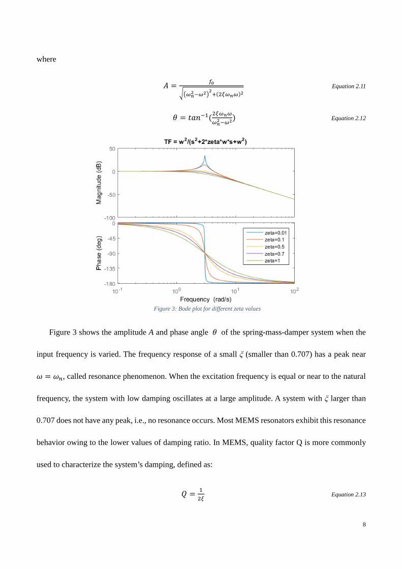
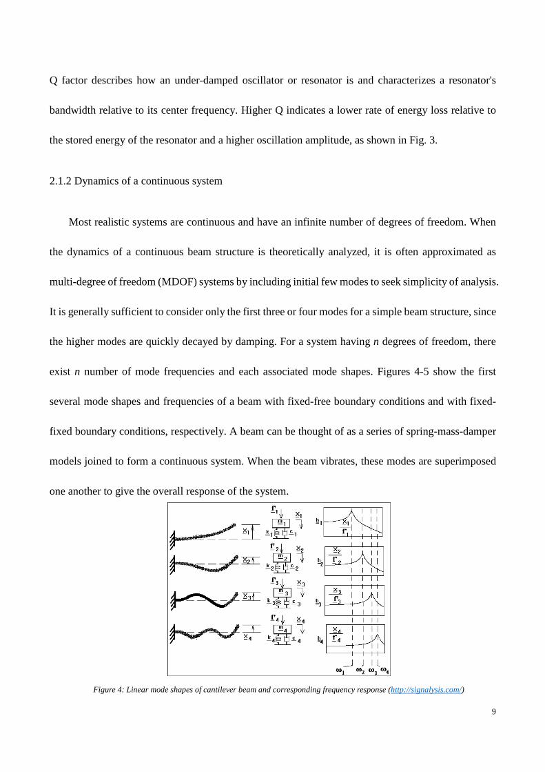
Most realistic systems are continuous and have an infinite number of degrees of freedom. When
the dynamics of a continuous beam structure is theoretically analyzed, it is often approximated as
multi-degree of freedom (MDOF) systems by including initial few modes to seek simplicity of analysis.
It is generally sufficient to consider only the first three or four modes for a simple beam structure, since
the higher modes are quickly decayed by damping. For a system having n degrees of freedom, there
exist n number of mode frequencies and each associated mode shapes. Figures 4-5 show the first
several mode shapes and frequencies of a beam with fixed-free boundary conditions and with fixed-
fixed boundary conditions, respectively. A beam can be thought of as a series of spring-mass-damper
models joined to form a continuous system. When the beam vibrates, these modes are superimposed
one another to give the overall response of the system.
Figure 4: Linear mode shapes of cantilever beam and corresponding frequency response (http://signalysis.com/)

10
Figure 5: Linear mode shape (1st, 2nd and 3rd modes) of a fixed-fixed beam
To derive the mode shape and mode frequency analytically, the beam structure should be modeled
more accurately as a continuous or distributed-parameter system of distributed mass, stiffness,
damping, and forcing. Its dynamical behavior is then governed by a partial differential equation that
vary in space and time as opposed to the ordinary differential equation in time like in the case of
lumped-parameter systems.
Figure 6: Free body diagram of a section of beam under transverse vibration
11
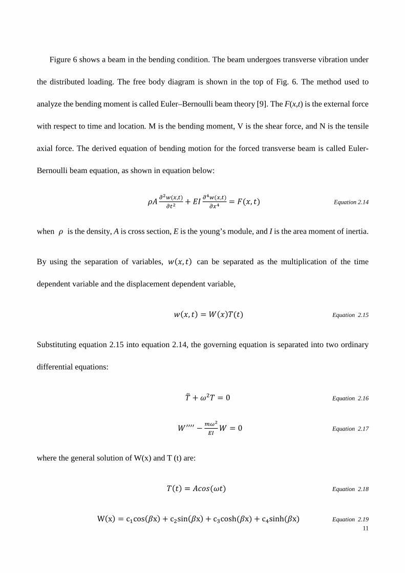
Figure 6 shows a beam in the bending condition. The beam undergoes transverse vibration under
the distributed loading. The free body diagram is shown in the top of Fig. 6. The method used to
analyze the bending moment is called Euler–Bernoulli beam theory [9]. The F(x,t) is the external force
with respect to time and location. M is the bending moment, V is the shear force, and N is the tensile
axial force. The derived equation of bending motion for the forced transverse beam is called Euler-
Bernoulli beam equation, as shown in equation below:
𝜌𝜌𝐴𝐴 𝜕𝜕2𝑤𝑤(𝑥𝑥,𝑡𝑡)𝜕𝜕𝑡𝑡2
+ 𝐸𝐸𝐸𝐸 𝜕𝜕4𝑤𝑤(𝑥𝑥,𝑡𝑡)𝜕𝜕𝑥𝑥4
= 𝐹𝐹(𝑥𝑥, 𝑡𝑡) Equation 2.14
when 𝜌𝜌 is the density, A is cross section, E is the young’s module, and I is the area moment of inertia.
By using the separation of variables, 𝑤𝑤(𝑥𝑥, 𝑡𝑡) can be separated as the multiplication of the time
dependent variable and the displacement dependent variable,
𝑤𝑤(𝑥𝑥, 𝑡𝑡) = 𝑊𝑊(𝑥𝑥)𝑇𝑇(𝑡𝑡) Equation 2.15
Substituting equation 2.15 into equation 2.14, the governing equation is separated into two ordinary
differential equations:
�̈�𝑇 + 𝜔𝜔2𝑇𝑇 = 0 Equation 2.16
𝑊𝑊′′′′ − 𝑚𝑚𝜔𝜔2
𝐸𝐸𝐸𝐸𝑊𝑊 = 0 Equation 2.17
where the general solution of W(x) and T (t) are:
𝑇𝑇(𝑡𝑡) = 𝐴𝐴𝑐𝑐𝑐𝑐𝑐𝑐(𝜔𝜔𝑡𝑡) Equation 2.18
W(x) = c1cos(𝛽𝛽x) + c2sin(𝛽𝛽x) + c3cosh(𝛽𝛽x) + c4sinh(𝛽𝛽x) Equation 2.19
12
Equation 2.19 is the mode shape function. c1, c2, c3, c4 and 𝛽𝛽 are constant which can be found by
applying the boundary conditions.
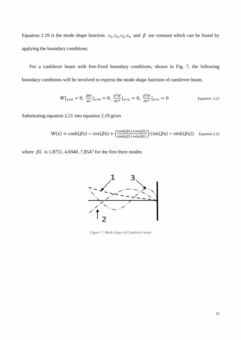
For a cantilever beam with free-fixed boundary conditions, shown in Fig. 7, the following
boundary conditions will be involved to express the mode shape function of cantilever beam.
𝑊𝑊|𝑥𝑥=0 = 0, 𝑑𝑑𝑑𝑑𝑑𝑑𝑥𝑥
|𝑥𝑥=0 = 0, 𝑑𝑑2𝑑𝑑𝑑𝑑𝑥𝑥2
|𝑥𝑥=𝐿𝐿 = 0, 𝑑𝑑3𝑑𝑑𝑑𝑑𝑥𝑥3
|𝑥𝑥=𝐿𝐿 = 0 Equation 2.21
Substituting equation 2.21 into equation 2.19 gives
W(x) = cosh(𝛽𝛽x) − cos(𝛽𝛽x) + �cosh(𝛽𝛽𝐿𝐿)+cos(𝛽𝛽𝐿𝐿)sinh(𝛽𝛽𝐿𝐿)+sin(𝛽𝛽𝐿𝐿)� (sin(𝛽𝛽x) − sinh(𝛽𝛽x)) Equation 2.22
where 𝛽𝛽𝛽𝛽 is 1.8751, 4.6940, 7,8547 for the first three modes.
Figure 7: Mode shape of Cantilever beam
13
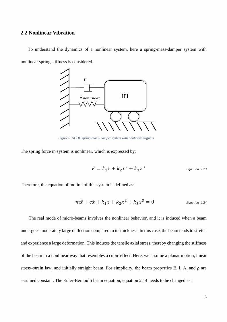
2.2 Nonlinear Vibration
To understand the dynamics of a nonlinear system, here a spring-mass-damper system with
nonlinear spring stiffness is considered.
The spring force in system is nonlinear, which is expressed by:
𝐹𝐹 = 𝑘𝑘1𝑥𝑥 + 𝑘𝑘2𝑥𝑥2 + 𝑘𝑘3𝑥𝑥3 Equation 2.23
Therefore, the equation of motion of this system is defined as:
𝑚𝑚�̈�𝑥 + 𝑐𝑐�̇�𝑥 + 𝑘𝑘1𝑥𝑥 + 𝑘𝑘2𝑥𝑥2 + 𝑘𝑘3𝑥𝑥3 = 0 Equation 2.24
The real mode of micro-beams involves the nonlinear behavior, and it is induced when a beam
undergoes moderately large deflection compared to its thickness. In this case, the beam tends to stretch
and experience a large deformation. This induces the tensile axial stress, thereby changing the stiffness
of the beam in a nonlinear way that resembles a cubic effect. Here, we assume a planar motion, linear
stress–strain law, and initially straight beam. For simplicity, the beam properties E, I, A, and ρ are
assumed constant. The Euler-Bernoulli beam equation, equation 2.14 needs to be changed as:
Figure 8: SDOF spring-mass- damper system with nonlinear stiffness
14
𝜌𝜌𝐴𝐴 𝜕𝜕2𝑤𝑤𝜕𝜕𝑡𝑡2
+ 𝐸𝐸𝐸𝐸 𝜕𝜕4𝑤𝑤𝜕𝜕𝑥𝑥4
= 𝑇𝑇 𝜕𝜕2𝑤𝑤𝜕𝜕𝑥𝑥2
+ 𝐹𝐹 Equation 2.21
where T is the tension in the beam. The tension is:
Δ𝐿𝐿𝐿𝐿
=∫ 𝑑𝑑𝑤𝑤�1+�𝜕𝜕𝑤𝑤𝜕𝜕𝑥𝑥�
2−𝛽𝛽𝛽𝛽
0
𝛽𝛽 Equation 2.22
𝑇𝑇 = 𝐸𝐸𝐴𝐴 Δ𝐿𝐿𝐿𝐿
= 𝐸𝐸𝐴𝐴2𝛽𝛽 ∫ 𝑑𝑑𝑤𝑤�𝜕𝜕𝑤𝑤𝜕𝜕𝑥𝑥�2𝛽𝛽
0 Equation 2.23
Substituting equation 2.22 and equation 2.23 into equation 2.21 will give the final expression of
nonlinear equation of motion:
ρA ∂2y∂t2
+ c ∂y∂t
+ EI ∂4y∂t4
− 𝐸𝐸𝐸𝐸2𝐿𝐿 ∫ 𝑑𝑑𝑑𝑑 �𝜕𝜕𝜕𝜕
𝜕𝜕𝑥𝑥�2𝐿𝐿
0 = Fcosωt Equation 2.24
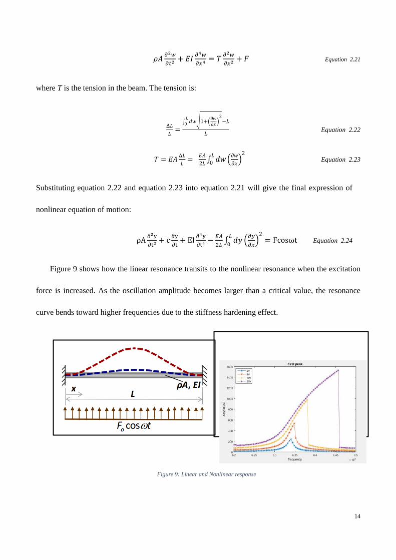
Figure 9 shows how the linear resonance transits to the nonlinear resonance when the excitation
force is increased. As the oscillation amplitude becomes larger than a critical value, the resonance
curve bends toward higher frequencies due to the stiffness hardening effect.
Figure 9: Linear and Nonlinear response
15
Chapter 3. Experiment Setup and Measurements
3.1 Experimental setup
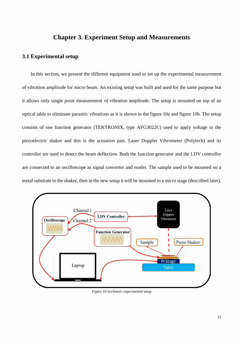
In this section, we present the different equipment used to set up the experimental measurement
of vibration amplitude for micro beam. An existing setup was built and used for the same purpose but
it allows only single point measurement of vibration amplitude. The setup is mounted on top of an
optical table to eliminate parasitic vibrations as it is shown in the figure 10a and figure 10b. The setup
consists of one function generator (TEKTRONIX, type AFG3022C) used to apply voltage to the
piezoelectric shaker and this is the actuation part. Laser Doppler Vibrometer (Polytech) and its
controller are used to detect the beam deflection. Both the function generator and the LDV controller
are connected to an oscilloscope as signal converter and reader. The sample used to be mounted on a
metal substrate to the shaker, then in the new setup it will be mounted to a micro stage (described later).
Figure 10:Sechmatic experimental setup
16
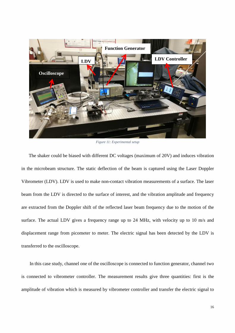
Figure 11: Experimental setup
The shaker could be biased with different DC voltages (maximum of 20V) and induces vibration
in the microbeam structure. The static deflection of the beam is captured using the Laser Doppler
Vibrometer (LDV). LDV is used to make non-contact vibration measurements of a surface. The laser
beam from the LDV is directed to the surface of interest, and the vibration amplitude and frequency
are extracted from the Doppler shift of the reflected laser beam frequency due to the motion of the
surface. The actual LDV gives a frequency range up to 24 MHz, with velocity up to 10 m/s and
displacement range from picometer to meter. The electric signal has been detected by the LDV is
transferred to the oscilloscope.
In this case study, channel one of the oscilloscope is connected to function generator, channel two
is connected to vibrometer controller. The measurement results give three quantities: first is the
amplitude of vibration which is measured by vibrometer controller and transfer the electric signal to
Function Generator
Oscilloscope
LDV LDV Controller
17
oscilloscope, and two phase shift, one is given by function generator and another is measured by
vibrometer controller. The difference between the two phases represent sample’s phase shift of
vibration. All the equipment are controlled using one LabVIEW program that allow to set the input
parameters and read the output data.
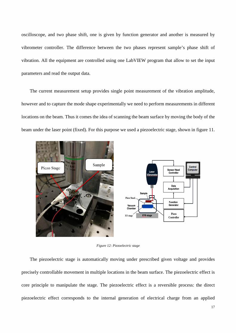
The current measurement setup provides single point measurement of the vibration amplitude,
however and to capture the mode shape experimentally we need to perform measurements in different
locations on the beam. Thus it comes the idea of scanning the beam surface by moving the body of the
beam under the laser point (fixed). For this purpose we used a piezoelectric stage, shown in figure 11.
Figure 12: Piezoelectric stage
The piezoelectric stage is automatically moving under prescribed given voltage and provides
precisely controllable movement in multiple locations in the beam surface. The piezoelectric effect is
core principle to manipulate the stage. The piezoelectric effect is a reversible process: the direct
piezoelectric effect corresponds to the internal generation of electrical charge from an applied
18
mechanical force, and the reverse piezoelectric effect consists of the internal generation of a
mechanical displacement under applied electrical field. The piezoelectric stage is fabricated by Physik
Instrumente (PI), type Q-522. It is 22 mm wide and 10 mm high and provides displacement within a
maximum travel range of 6.5mm and with a resolution (smallest displacement) down to 4nm. The
velocity of stage is up to 10 mm/ s. and it can hold 1 N force.
LabVIEW [10] software is used to control the stage movement as well as the input/output signals
thus the communication between the equipment and the computer. The software consists of a collection
of virtual instrument (VI) drivers. All functionalities involves one or more VIs with the appropriate
parameters and variables settings.
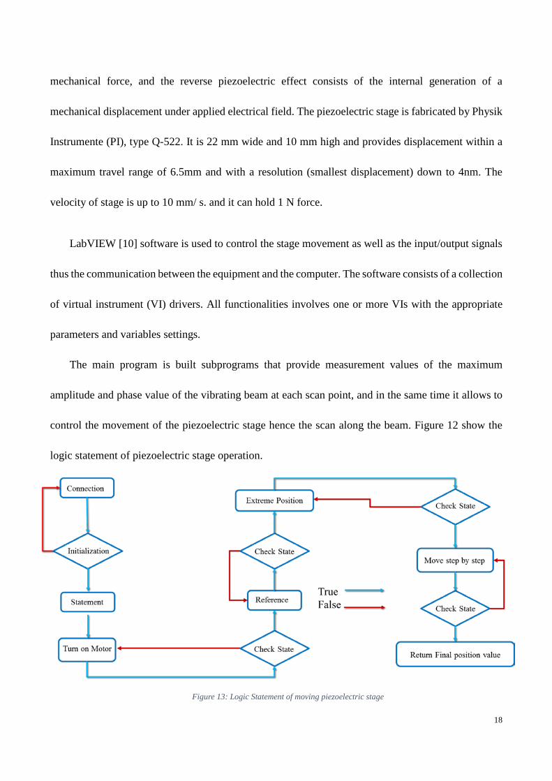
The main program is built subprograms that provide measurement values of the maximum
amplitude and phase value of the vibrating beam at each scan point, and in the same time it allows to
control the movement of the piezoelectric stage hence the scan along the beam. Figure 12 show the
logic statement of piezoelectric stage operation.
Figure 12: Figure 13: Logic Statement of moving piezoelectric stage
19
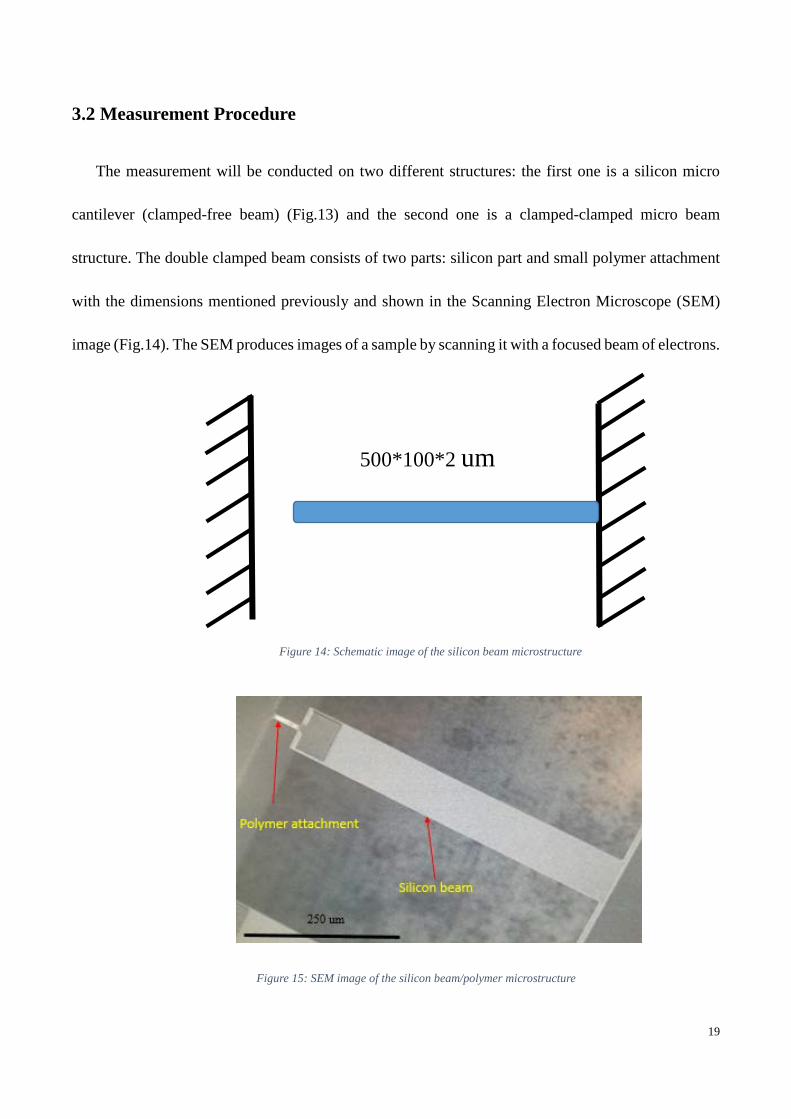
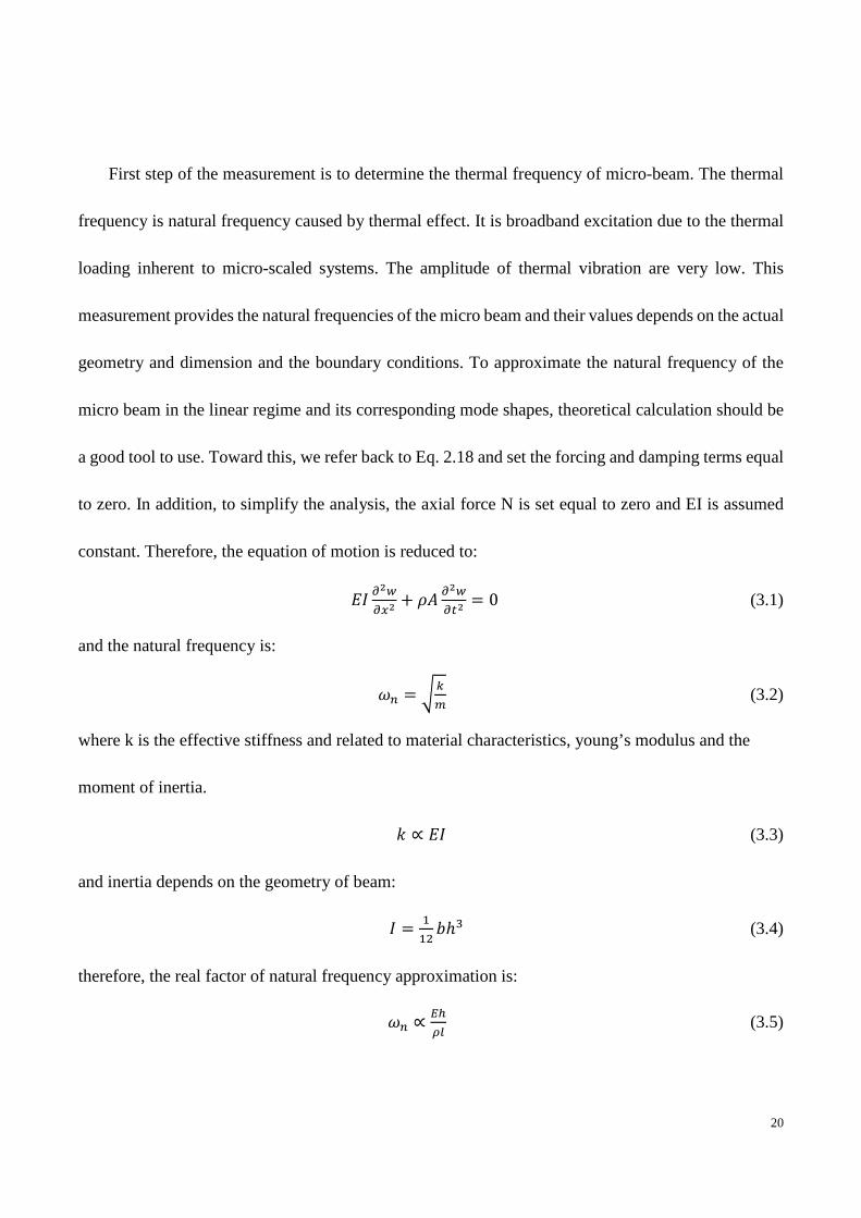
3.2 Measurement Procedure
The measurement will be conducted on two different structures: the first one is a silicon micro
cantilever (clamped-free beam) (Fig.13) and the second one is a clamped-clamped micro beam
structure. The double clamped beam consists of two parts: silicon part and small polymer attachment
with the dimensions mentioned previously and shown in the Scanning Electron Microscope (SEM)
image (Fig.14). The SEM produces images of a sample by scanning it with a focused beam of electrons.
500*100*2 um
Figure 14: Schematic image of the silicon beam microstructure
Figure 15: SEM image of the silicon beam/polymer microstructure
20
First step of the measurement is to determine the thermal frequency of micro-beam. The thermal
frequency is natural frequency caused by thermal effect. It is broadband excitation due to the thermal
loading inherent to micro-scaled systems. The amplitude of thermal vibration are very low. This
measurement provides the natural frequencies of the micro beam and their values depends on the actual
geometry and dimension and the boundary conditions. To approximate the natural frequency of the
micro beam in the linear regime and its corresponding mode shapes, theoretical calculation should be
a good tool to use. Toward this, we refer back to Eq. 2.18 and set the forcing and damping terms equal
to zero. In addition, to simplify the analysis, the axial force N is set equal to zero and EI is assumed
constant. Therefore, the equation of motion is reduced to:
𝐸𝐸𝐸𝐸 𝜕𝜕2𝑤𝑤𝜕𝜕𝑥𝑥2
+ 𝜌𝜌𝐴𝐴 𝜕𝜕2𝑤𝑤𝜕𝜕𝑡𝑡2
= 0 (3.1)
and the natural frequency is:
𝜔𝜔𝑛𝑛 = �𝑘𝑘𝑚𝑚
(3.2)
where k is the effective stiffness and related to material characteristics, young’s modulus and the
moment of inertia.
𝑘𝑘 ∝ 𝐸𝐸𝐸𝐸 (3.3)
and inertia depends on the geometry of beam:
𝐸𝐸 = 112𝑏𝑏ℎ3 (3.4)
therefore, the real factor of natural frequency approximation is:
𝜔𝜔𝑛𝑛 ∝𝐸𝐸ℎ𝜌𝜌𝜌𝜌
(3.5)
21
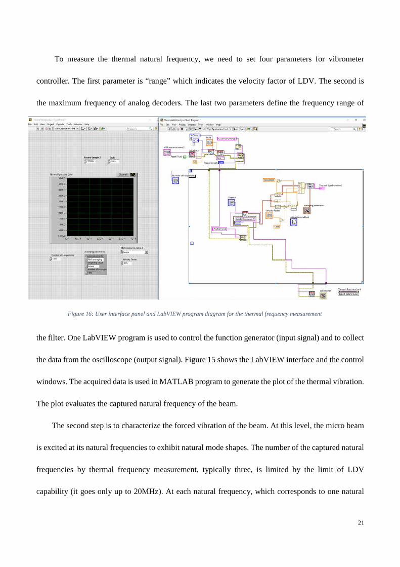
To measure the thermal natural frequency, we need to set four parameters for vibrometer
controller. The first parameter is “range” which indicates the velocity factor of LDV. The second is
the maximum frequency of analog decoders. The last two parameters define the frequency range of
the filter. One LabVIEW program is used to control the function generator (input signal) and to collect
the data from the oscilloscope (output signal). Figure 15 shows the LabVIEW interface and the control
windows. The acquired data is used in MATLAB program to generate the plot of the thermal vibration.
The plot evaluates the captured natural frequency of the beam.
The second step is to characterize the forced vibration of the beam. At this level, the micro beam
is excited at its natural frequencies to exhibit natural mode shapes. The number of the captured natural
frequencies by thermal frequency measurement, typically three, is limited by the limit of LDV
capability (it goes only up to 20MHz). At each natural frequency, which corresponds to one natural
Figure 16: User interface panel and LabVIEW program diagram for the thermal frequency measurement
22
mode shape, the frequency response and the vibration amplitude measurement were performed at
different locations in the beam using the new capability of the setup.
Here as we add the moving stage, a sub program has been added to the main LabVIEW program
to manipulate the stage during measurement. Once everything is integrated, the new setup controlled
with the new LabVIEW program makes possible the measurement of the dynamic response of the
beam at different locations of the beam geometry. The measurement is continuous and stages are
moving automatically for the next location (measurement point). The moving step is defined by giving
the length of the beam and the number of points that will be covered. The custom LabVIEW will be
introduced in Chapter 4.
23
Chapter 4: Results and Discussion
This Chapter covers two main parts: The first part describes the components and the steps to
follow to build the control of the stages as an added value to the measurement procedure. In the
second part the dynamic response measurement and mode shape are presented for two micro beams.
4.1 LabVIEW Programs
4.1.1 User Panel
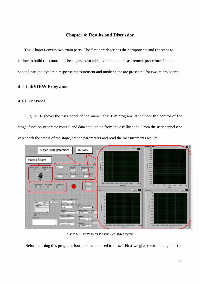
Figure 16 shows the user panel of the main LabVIEW program. It includes the control of the
stage, function generator control and data acquisition from the oscilloscope. From the user pannel one
can check the status of the stage, set the parameters and read the measurements results.
Figure 17: User Panel for the main LabVIEW program
Before running this program, four parameters need to be set. First we give the total length of the
24
microbeam in micrometer. The sign of value must be included because it indicates the orientation of
moving stage. Positive sign indicates that the stage is moving to the right from starting point, and to
the left at negative sign. The second parameter is the total scanning points N and it should be an integer.
This value tells the stage how many movement needs to be achieved and it corresponds to N-1 steps.
The step between two movements is calculated as the quotient of total length by total number of
movement. The third parameter is the velocity factor which controls the vibrometer measurement. The
last parameter is the frequency and it corresponds to one natural frequency of the beam. The value of
the frequency indicates the mode frequency of the sample. This number is used to calculate two values
of output, maximum amplitude value and phase value. The frequency response curve is also provided
at each point measurement. When running the LabVIEW program, the delay time between moving the
stage and measuring can be controlled.
4.1.2 Stage Controller Program
This section describes how to build custom LabVIEW program to control PI stage. This program
is integrate in the main LabVIEW program (described earlier) to run the experiment.
The first step is running ‘E873_Configuration_Setup.vi’. This sub vi file will initialize vi with all
necessary steps automatically. Then the following steps are performed in order: 1. Open the
communications port. 2. Define the IDs for the connected axes. 3. Set references to the connected
stages (if appropriate), depending on if the controller requires a referencing before axes can be moved
and on your custom settings. 4. Define the controller name. After these steps, parameters are saved in
global variables, so that other vis invoked during the same LabVIEW session can access this data at
runtime. For successful run, we select the flowing setting shown in table 1. After running
25
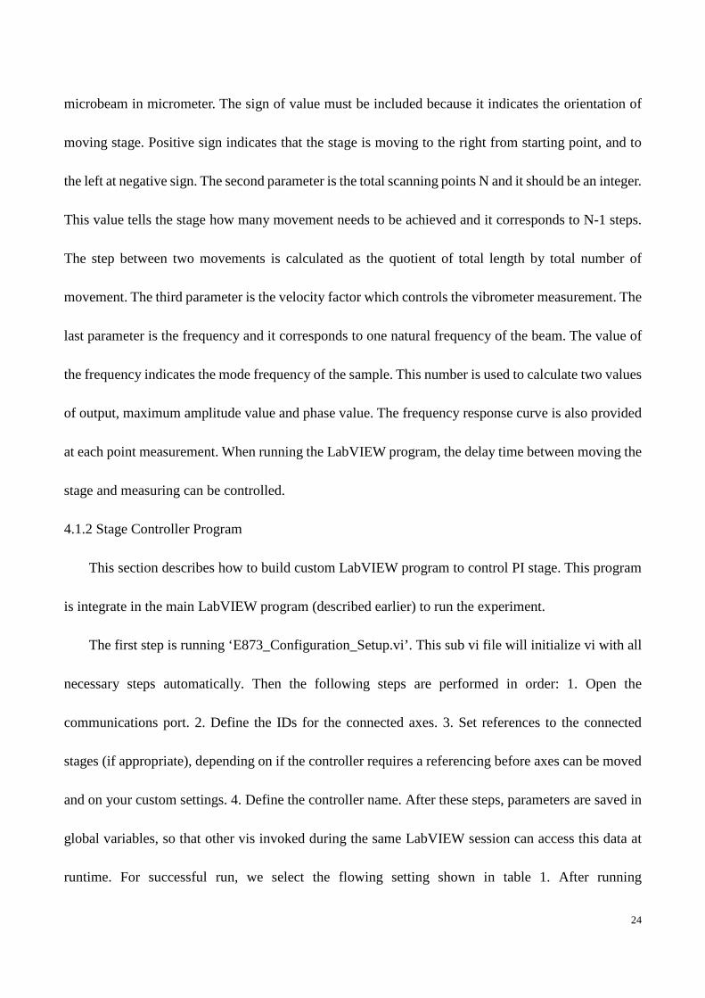
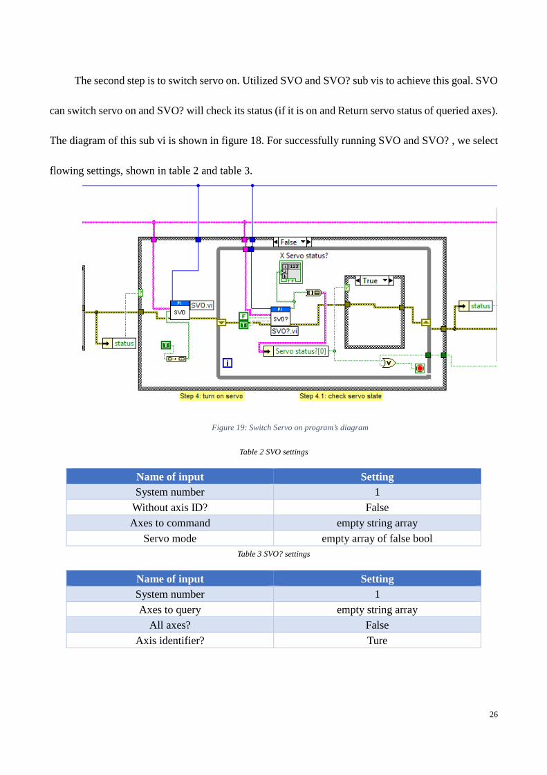
‘E873_Configuration_Setup.vi’, this sub vi will communicate one cluster to the next sub vi which
contain three elements, status, code and source. The other sub vis will do the same assignment and
pass one cluster to the next sub vi function. Figure 17 shows the diagram of
“E873_Configuration_Setup.vi” and its different components.
Table 1 E873_Configuration_Setup value
Name of Input Setting Function
Interface Settings Multiple value, shown in Fig,22
System number 1 The 1 refers to the axis Referencing FRF To reference the stage
Interface USB All axes? F Only one axes
Axes to move 1 Stage selection Multiple value, shown in Fig,22
Switch servo on? F Only check status of stage
Interface Settings
Stage selection
Figure 18: E873_Configuration_Setup.vi
26
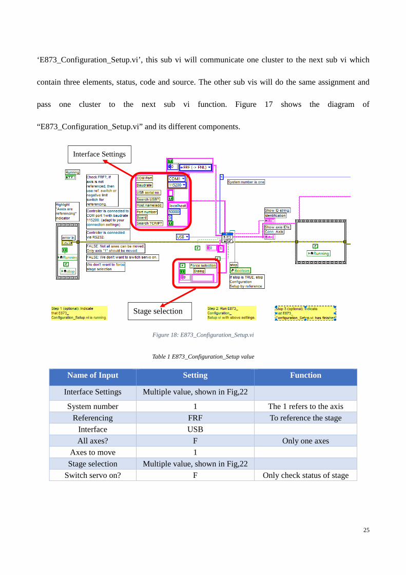
The second step is to switch servo on. Utilized SVO and SVO? sub vis to achieve this goal. SVO
can switch servo on and SVO? will check its status (if it is on and Return servo status of queried axes).
The diagram of this sub vi is shown in figure 18. For successfully running SVO and SVO? , we select
flowing settings, shown in table 2 and table 3.
Table 2 SVO settings
Name of input Setting System number 1
Without axis ID? False Axes to command empty string array
Servo mode empty array of false bool Table 3 SVO? settings
Name of input Setting System number 1 Axes to query empty string array
All axes? False Axis identifier? Ture
Figure 19: Switch Servo on program’s diagram
27
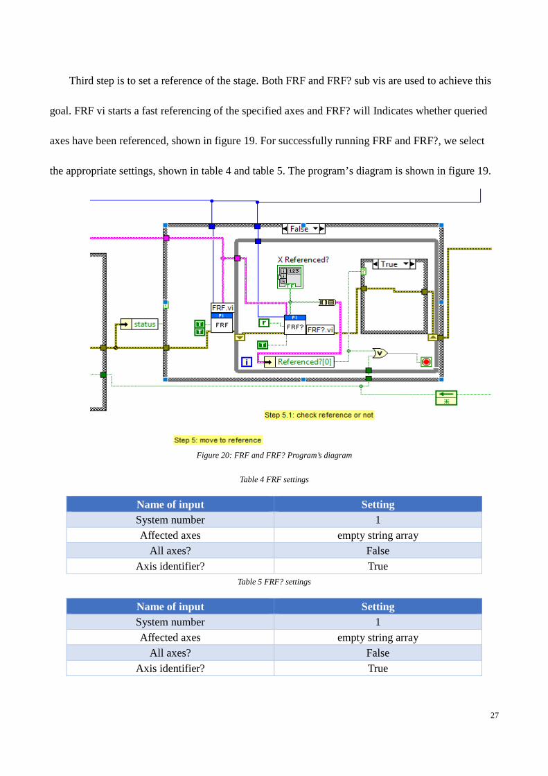
Third step is to set a reference of the stage. Both FRF and FRF? sub vis are used to achieve this
goal. FRF vi starts a fast referencing of the specified axes and FRF? will Indicates whether queried
axes have been referenced, shown in figure 19. For successfully running FRF and FRF?, we select
the appropriate settings, shown in table 4 and table 5. The program’s diagram is shown in figure 19.
Figure 20: FRF and FRF? Program’s diagram
Table 4 FRF settings
Name of input Setting System number 1 Affected axes empty string array
All axes? False Axis identifier? True
Table 5 FRF? settings
Name of input Setting System number 1 Affected axes empty string array
All axes? False Axis identifier? True
28
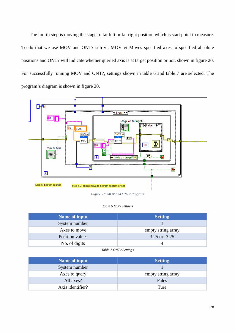
The fourth step is moving the stage to far left or far right position which is start point to measure.
To do that we use MOV and ONT? sub vi. MOV vi Moves specified axes to specified absolute
positions and ONT? will indicate whether queried axis is at target position or not, shown in figure 20.
For successfully running MOV and ONT?, settings shown in table 6 and table 7 are selected. The
program’s diagram is shown in figure 20.
Table 6 MOV settings
Name of input Setting System number 1 Axes to move empty string array
Position values 3.25 or -3.25 No. of digits 4
Table 7 ONT? Settings
Name of input Setting System number 1 Axes to query empty string array
All axes? Fales Axis identifier? Ture
Figure 21: MOV and ONT? Program
29
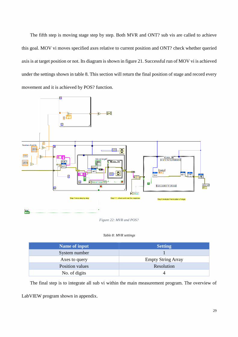
The fifth step is moving stage step by step. Both MVR and ONT? sub vis are called to achieve
this goal. MOV vi moves specified axes relative to current position and ONT? check whether queried
axis is at target position or not. Its diagram is shown in figure 21. Successful run of MOV vi is achieved
under the settings shown in table 8. This section will return the final position of stage and record every
movement and it is achieved by POS? function.
Table 8: MVR settings
Name of input Setting System number 1 Axes to query Empty String Array Position values Resolution
No. of digits 4
The final step is to integrate all sub vi within the main measurement program. The overview of
LabVIEW program shown in appendix.
Figure 22: MVR and POS?
30
4.2. Experimental results and processed data:
4.2.1 Micro cantilever beam
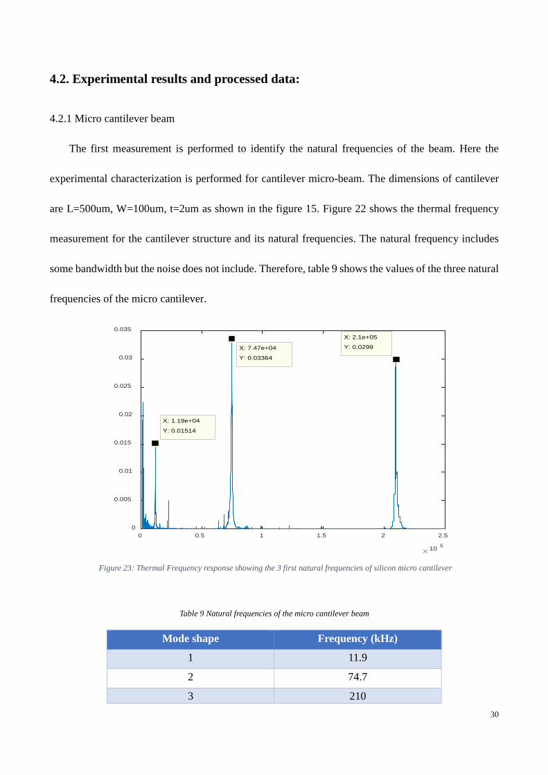
The first measurement is performed to identify the natural frequencies of the beam. Here the
experimental characterization is performed for cantilever micro-beam. The dimensions of cantilever
are L=500um, W=100um, t=2um as shown in the figure 15. Figure 22 shows the thermal frequency
measurement for the cantilever structure and its natural frequencies. The natural frequency includes
some bandwidth but the noise does not include. Therefore, table 9 shows the values of the three natural
frequencies of the micro cantilever.
Table 9 Natural frequencies of the micro cantilever beam
Mode shape Frequency (kHz)
1 11.9
2 74.7
3 210
10 5
0 0.5 1 1.5 2 2.50
0.005
0.01
0.015
0.02
0.025
0.03
0.035
X: 1.19e+04
Y: 0.01514
X: 7.47e+04
Y: 0.03364
X: 2.1e+05
Y: 0.0299
Figure 23: Thermal Frequency response showing the 3 first natural frequencies of silicon micro cantilever
31
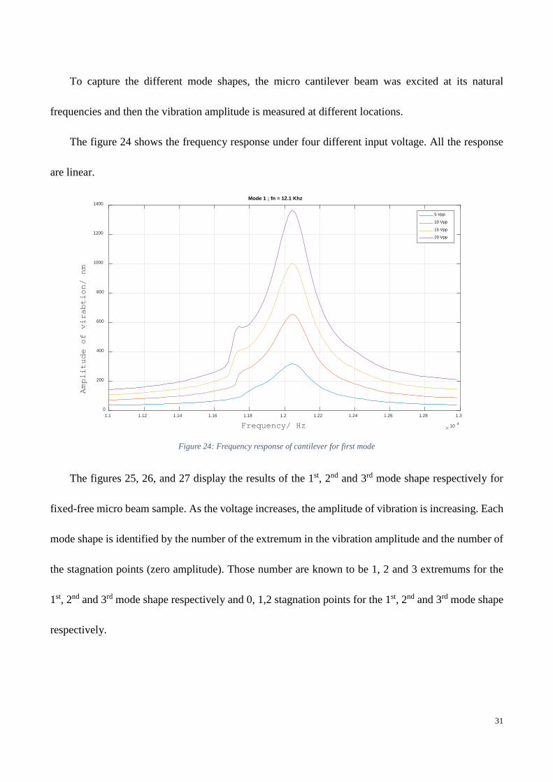
To capture the different mode shapes, the micro cantilever beam was excited at its natural
frequencies and then the vibration amplitude is measured at different locations.
The figure 24 shows the frequency response under four different input voltage. All the response
are linear.
Figure 24: Frequency response of cantilever for first mode
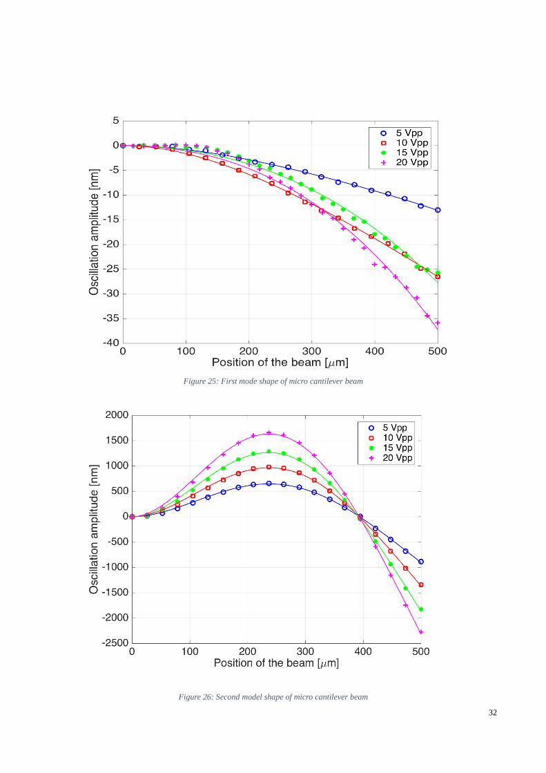
The figures 25, 26, and 27 display the results of the 1st, 2nd and 3rd mode shape respectively for
fixed-free micro beam sample. As the voltage increases, the amplitude of vibration is increasing. Each
mode shape is identified by the number of the extremum in the vibration amplitude and the number of
the stagnation points (zero amplitude). Those number are known to be 1, 2 and 3 extremums for the
1st, 2nd and 3rd mode shape respectively and 0, 1,2 stagnation points for the 1st, 2nd and 3rd mode shape
respectively.
1.1 1.12 1.14 1.16 1.18 1.2 1.22 1.24 1.26 1.28 1.3
Frequency/ Hz 10 4
0
200
400
600
800
1000
1200
1400
Amplitude of virabtion/ nm
Mode 1 ; fn = 12.1 Khz
5 Vpp
10 Vpp
15 Vpp
20 Vpp
32
Figure 25: First mode shape of micro cantilever beam
Figure 26: Second model shape of micro cantilever beam
33
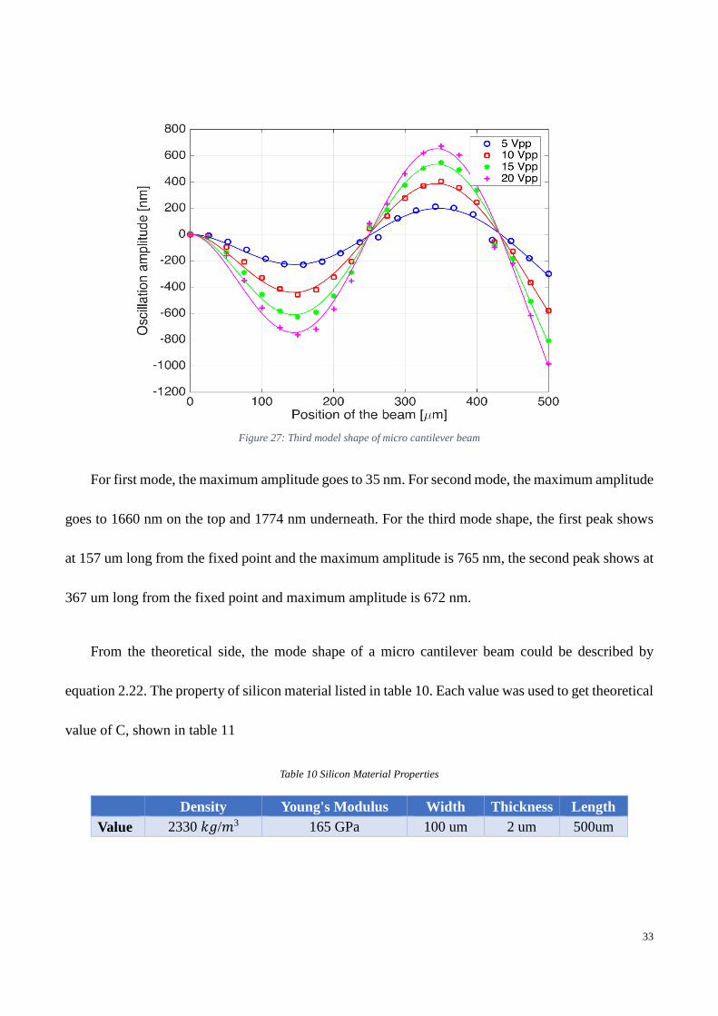
Figure 27: Third model shape of micro cantilever beam
For first mode, the maximum amplitude goes to 35 nm. For second mode, the maximum amplitude
goes to 1660 nm on the top and 1774 nm underneath. For the third mode shape, the first peak shows
at 157 um long from the fixed point and the maximum amplitude is 765 nm, the second peak shows at
367 um long from the fixed point and maximum amplitude is 672 nm.
From the theoretical side, the mode shape of a micro cantilever beam could be described by
equation 2.22. The property of silicon material listed in table 10. Each value was used to get theoretical
value of C, shown in table 11
Table 10 Silicon Material Properties
Density Young's Modulus Width Thickness Length Value 2330 𝑘𝑘𝑘𝑘/𝑚𝑚3 165 GPa 100 um 2 um 500um
34
Table 11 Theoretical coefficient value of c
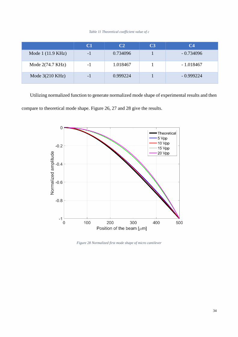
Utilizing normalized function to generate normalized mode shape of experimental results and then
compare to theoretical mode shape. Figure 26, 27 and 28 give the results.
C1 C2 C3 C4
Mode 1 (11.9 KHz) -1 0.734096 1 - 0.734096
Mode 2(74.7 KHz) -1 1.018467 1 - 1.018467
Mode 3(210 KHz) -1 0.999224 1 - 0.999224
Figure 28 Normalized first mode shape of micro cantilever
35
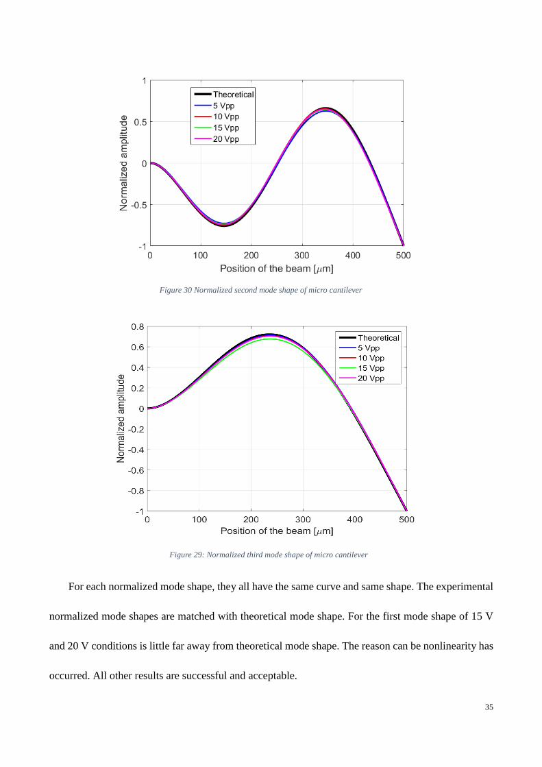
For each normalized mode shape, they all have the same curve and same shape. The experimental
normalized mode shapes are matched with theoretical mode shape. For the first mode shape of 15 V
and 20 V conditions is little far away from theoretical mode shape. The reason can be nonlinearity has
occurred. All other results are successful and acceptable.
Figure 30 Normalized second mode shape of micro cantilever
Figure 29: Normalized third mode shape of micro cantilever
36
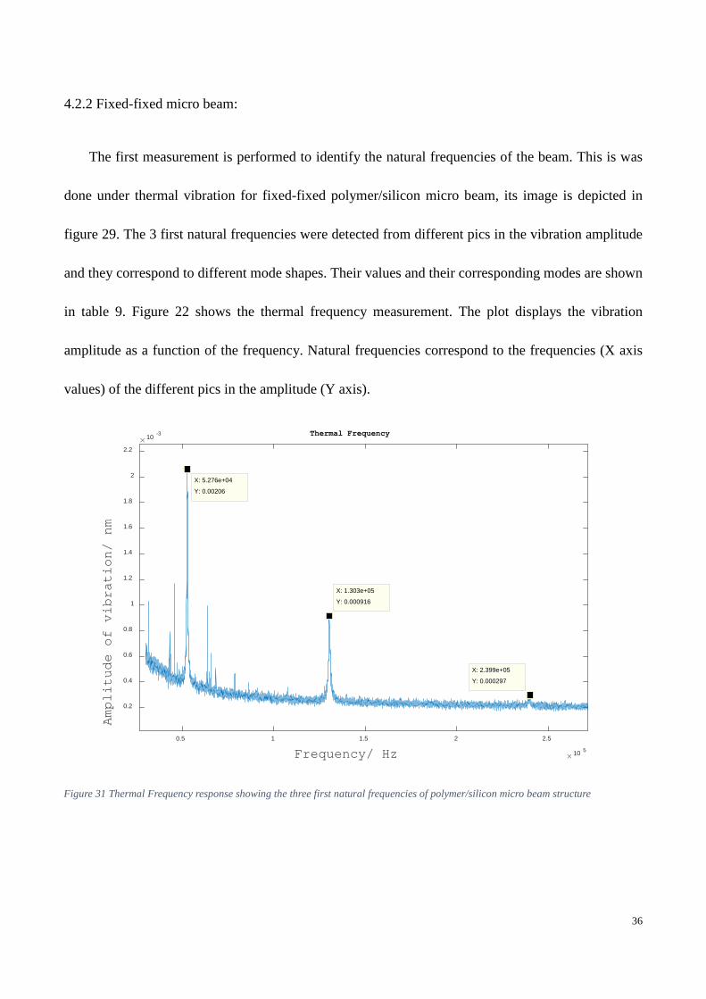
4.2.2 Fixed-fixed micro beam:
The first measurement is performed to identify the natural frequencies of the beam. This is was
done under thermal vibration for fixed-fixed polymer/silicon micro beam, its image is depicted in
figure 29. The 3 first natural frequencies were detected from different pics in the vibration amplitude
and they correspond to different mode shapes. Their values and their corresponding modes are shown
in table 9. Figure 22 shows the thermal frequency measurement. The plot displays the vibration
amplitude as a function of the frequency. Natural frequencies correspond to the frequencies (X axis
values) of the different pics in the amplitude (Y axis).
Figure 31 Thermal Frequency response showing the three first natural frequencies of polymer/silicon micro beam structure
0.5 1 1.5 2 2.5
Frequency/ Hz 10 5
0.2
0.4
0.6
0.8
1
1.2
1.4
1.6
1.8
2
2.2
Amplitude of vibration/ nm
10 -3 Thermal Frequency
X: 5.276e+04
Y: 0.00206
X: 1.303e+05
Y: 0.000916
X: 2.399e+05
Y: 0.000297
37
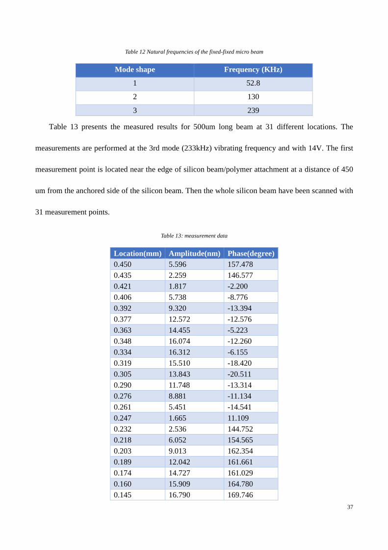
Table 12 Natural frequencies of the fixed-fixed micro beam
Mode shape Frequency (KHz)
1 52.8
2 130
3 239
Table 13 presents the measured results for 500um long beam at 31 different locations. The
measurements are performed at the 3rd mode (233kHz) vibrating frequency and with 14V. The first
measurement point is located near the edge of silicon beam/polymer attachment at a distance of 450
um from the anchored side of the silicon beam. Then the whole silicon beam have been scanned with
31 measurement points.
Table 13: measurement data
Location(mm) Amplitude(nm) Phase(degree) 0.450 5.596 157.478 0.435 2.259 146.577 0.421 1.817 -2.200 0.406 5.738 -8.776 0.392 9.320 -13.394 0.377 12.572 -12.576 0.363 14.455 -5.223 0.348 16.074 -12.260 0.334 16.312 -6.155 0.319 15.510 -18.420 0.305 13.843 -20.511 0.290 11.748 -13.314 0.276 8.881 -11.134 0.261 5.451 -14.541 0.247 1.665 11.109 0.232 2.536 144.752 0.218 6.052 154.565 0.203 9.013 162.354 0.189 12.042 161.661 0.174 14.727 161.029 0.160 15.909 164.780 0.145 16.790 169.746
38
0.131 17.069 163.774 0.116 16.437 164.740 0.102 14.855 173.716 0.087 12.709 165.292 0.073 10.530 165.077 0.058 7.766 162.938 0.044 5.168 166.067 0.029 2.627 155.626 0.015 0.626 151.967 0 0 0
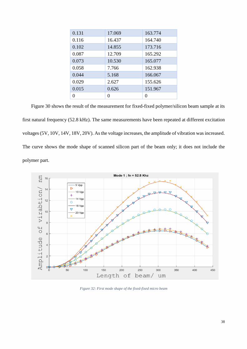
Figure 30 shows the result of the measurement for fixed-fixed polymer/silicon beam sample at its
first natural frequency (52.8 kHz). The same measurements have been repeated at different excitation
voltages (5V, 10V, 14V, 18V, 20V). As the voltage increases, the amplitude of vibration was increased.
The curve shows the mode shape of scanned silicon part of the beam only; it does not include the
polymer part.
Figure 32: First mode shape of the fixed-fixed micro beam
39
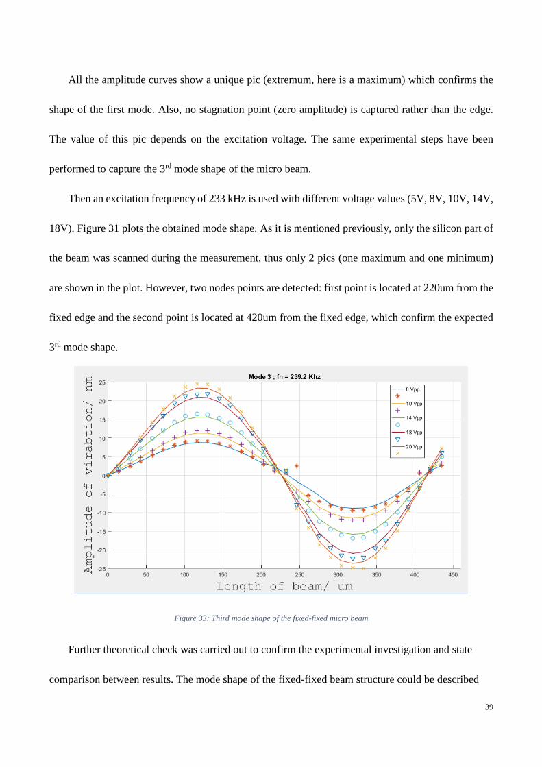
All the amplitude curves show a unique pic (extremum, here is a maximum) which confirms the
shape of the first mode. Also, no stagnation point (zero amplitude) is captured rather than the edge.
The value of this pic depends on the excitation voltage. The same experimental steps have been
performed to capture the 3rd mode shape of the micro beam.
Then an excitation frequency of 233 kHz is used with different voltage values (5V, 8V, 10V, 14V,
18V). Figure 31 plots the obtained mode shape. As it is mentioned previously, only the silicon part of
the beam was scanned during the measurement, thus only 2 pics (one maximum and one minimum)
are shown in the plot. However, two nodes points are detected: first point is located at 220um from the
fixed edge and the second point is located at 420um from the fixed edge, which confirm the expected
3rd mode shape.
Figure 33: Third mode shape of the fixed-fixed micro beam
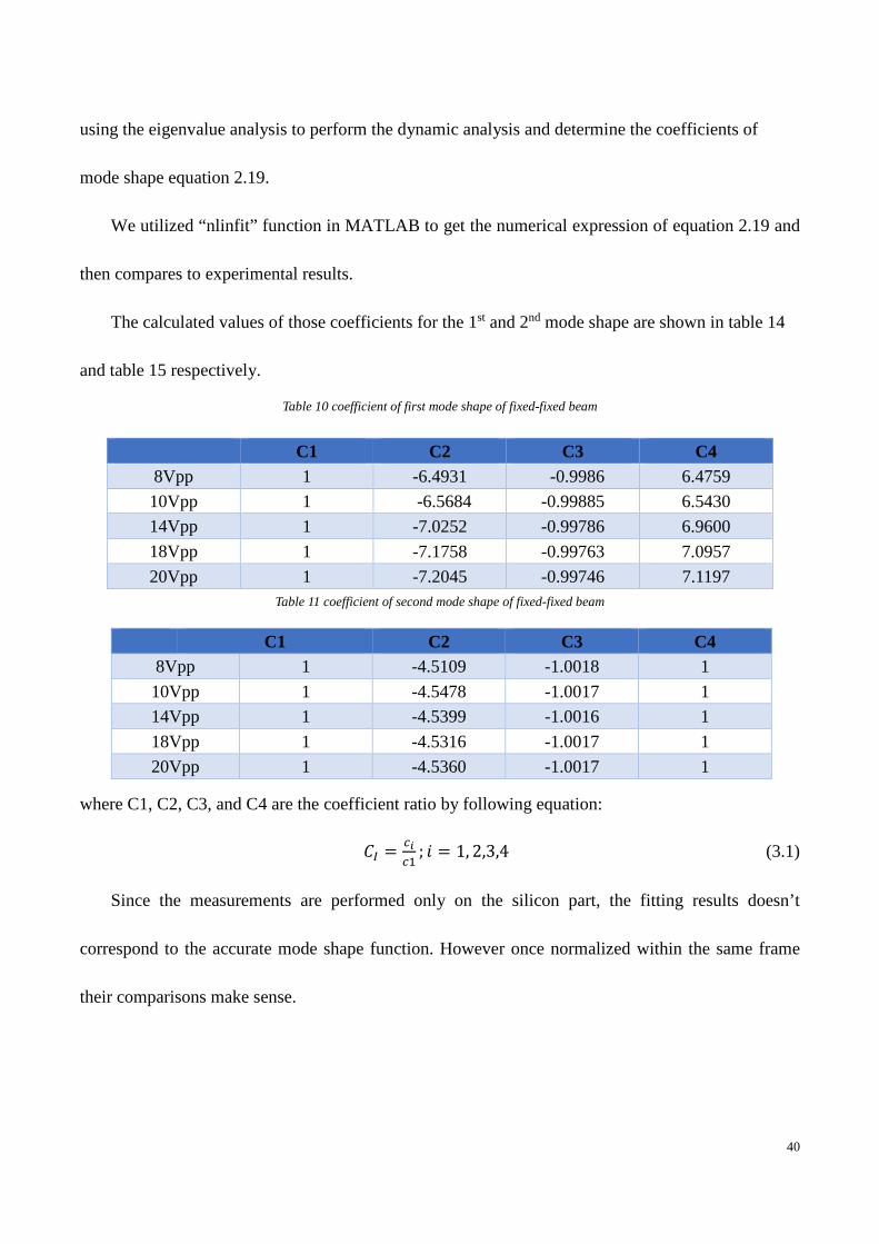
Further theoretical check was carried out to confirm the experimental investigation and state
comparison between results. The mode shape of the fixed-fixed beam structure could be described
40
using the eigenvalue analysis to perform the dynamic analysis and determine the coefficients of
mode shape equation 2.19.
We utilized “nlinfit” function in MATLAB to get the numerical expression of equation 2.19 and
then compares to experimental results.
The calculated values of those coefficients for the 1st and 2nd mode shape are shown in table 14
and table 15 respectively.
Table 10 coefficient of first mode shape of fixed-fixed beam
Table 11 coefficient of second mode shape of fixed-fixed beam
C1 C2 C3 C4 8Vpp 1 -4.5109 -1.0018 1 10Vpp 1 -4.5478 -1.0017 1 14Vpp 1 -4.5399 -1.0016 1 18Vpp 1 -4.5316 -1.0017 1 20Vpp 1 -4.5360 -1.0017 1
where C1, C2, C3, and C4 are the coefficient ratio by following equation:
𝐶𝐶𝐸𝐸 = 𝑐𝑐𝑖𝑖𝑐𝑐1
; 𝐵𝐵 = 1, 2,3,4 (3.1)
Since the measurements are performed only on the silicon part, the fitting results doesn’t
correspond to the accurate mode shape function. However once normalized within the same frame
their comparisons make sense.
C1 C2 C3 C4 8Vpp 1 -6.4931 -0.9986 6.4759 10Vpp 1 -6.5684 -0.99885 6.5430 14Vpp 1 -7.0252 -0.99786 6.9600 18Vpp 1 -7.1758 -0.99763 7.0957 20Vpp 1 -7.2045 -0.99746 7.1197

41
Chapter 5: Conclusion and Future Works
This research presents an experimental identification of mode shapes for vibrating micro beam.
However, a theoretical study of the linear and nonlinear vibration regimes has been covered as well.
As a start point, an old experimental setup has been and this allows only single point measurement
which was not enough to build the mode shape of the structure. Then most part of this research was
allocated to build an automatic measurement setup that covers different locations in the structure
geometry. The requirement was to custom a general and flexible LabVIEW control program. The
design of the setup takes in consideration the limitations and the sensitivity of the stage and a minimum
step size of 4nm is allowable which is very accurate for micro scale structures.
As accuracy is concerned, as we increase the number of the scanned point as clear and more
defined the mode shape is. Also here only the scan in the X axis is presented which draws only 1D
(line) mode shape, however combining the measurements in two axes (X and Y) will provide a 2D
(surface) images of the mode shape.
Giving the size of the moving stage, the actual measurements were conducted in ambient air
condition which increase the error factor and add unwanted factors specially the air damping. Thus a
further work will be carried out to perform the experiment in large vacuum chamber in order to exclude
external factors. Different results is expected to be generated and would be more accurate
42
References
[1] Y. Développement, "MEMS Markets Status of the MEMS Industry 2015.," 2015. [2] Z. S. a. I. Stanimirović, "Mechanical Properties of MEMS Materials," December 1, 2009. [3] "MEMS Sensors for automotive appkications, life.augmented," [Online]. Available:
http://www.st.com/en/mems-and-sensors.html. [4] "MEMS in Healthcare," [Online]. Available: http://www.eeherald.com/section/design-
guide/mems_medical.html. [5] H. X. T. &. M. L. R. Mo Li1, "Ultra-sensitive NEMS-based cantilevers for sensing, scanned
probe and very high-frequency applications," Nature Nanotechnology, 2007. [6] "Introduction to Microelectromechanical Systems (MEMS)," [Online]. Available:
https://compliantmechanisms.byu.edu/content/introduction-microelectromechanical-systems-mems.
[7] T. I. T. R. f. Semiconductors, "Micro-Electro-Mechanical Systems (MEMS)," 2013. [8] R. L. a. M. C. Cross, "Nonlinear Dynamics of Nanomechanical and Micromechanical
Resonators". [9] L. G. Villanueva, "Nonlinearity in nanomechanical cantilever," 2013. [10] LabVIEW (Vison 2015).

43
Appendix:
Custom LabVIEW part 1
44
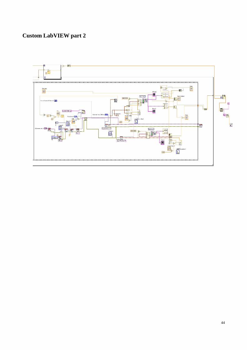
Custom LabVIEW part 2
45
MATLAB code for free-fixed beam clc;clear all; close all; load V5test1.txt load V10test1.txt load V15test1.txt load V20test1.txt L=0.5; %[mm] %% 5V L5 = V5test1(:,1); A5 = V5test1(:,2); P5 = V5test1(:,3); n5 = length(P5); for i = 1:n5 if P5(i)<=0 A5(i)=-A5(i); end if P5(i)>0 A5(i)=A5(i); end end A5 = (A5-A5(1)); L5 = (L5-L5(1))/(L5(n5)-L5(1))*L; c50 = [max(abs(A5))/2 9.388 1]; modelfun5 = @(c5,x)c5(1)*(-cos(c5(2)*x)+c5(3)*sin(c5(2)*x)+1*cosh(c5(2)*x)-
c5(3)*sinh(c5(2)*x)); c5f = nlinfit(L5,A5,modelfun5,c50); %% 10V L10 = V10test1(:,1); A10 = V10test1(:,2); P10 = V10test1(:,3); n10 = length(P10);
46
for i = 1:n10 if P10(i)<=0 A10(i)=-A10(i); end if P10(i)>0 A10(i)=A10(i); end end A10 = (A10-A10(1)); L10 = (L10-L10(1))/(L10(n10)-L10(1))*L; c100 = [max(abs(A10))/2 9.388 1]; modelfun10 = @(c10,x)c10(1)*(-
cos(c10(2)*x)+c10(3)*sin(c10(2)*x)+1*cosh(c10(2)*x)-c10(3)*sinh(c10(2)*x)); c10f = nlinfit(L10,A10,modelfun10,c100); %% 15 L15 = V15test1(:,1); A15 = V15test1(:,2); P15 = V15test1(:,3); n15 = length(P15); for i = 1:n15 if P15(i)<=0 A15(i)=-A15(i); end if P15(i)>0 A15(i)=A15(i); end end A15 = (A15-A15(1)); L15 = (L15-L15(1))/(L15(n15)-L15(1))*L; c150 = [max(abs(A15))/2 9.388 1]; modelfun15 = @(c15,x)c15(1)*(-
cos(c15(2)*x)+c15(3)*sin(c15(2)*x)+1*cosh(c15(2)*x)-c15(3)*sinh(c15(2)*x));
47
c15f = nlinfit(L15,A15,modelfun15,c150); %% L20 = V20test1(:,1); A20 = V20test1(:,2); P20 = V20test1(:,3); n20 = length(P20); for i = 1:n20 if P20(i)<=0 A20(i)=-A20(i); end if P20(i)>0 A20(i)=A20(i); end end A20 = (A20-A20(1)); L20 = (L20-L20(1))/(L20(n20)-L20(1))*L; c200 = [max(abs(A20))/2 9.388 1]; modelfun20 = @(c20,x)c20(1)*(-
cos(c20(2)*x)+c20(3)*sin(c20(2)*x)+1*cosh(c20(2)*x)-c20(3)*sinh(c20(2)*x)); c20f = nlinfit(L20,A20,modelfun20,c200) %% figure(1) figure(1) % experimental data plot(L5*1000,A5,'bo','LineWidth',2, 'MarkerSize',7); hold on plot(L10*1000,A10,'rs','LineWidth',2, 'MarkerSize',7) plot(L15*1000,A15,'g*','LineWidth',2, 'MarkerSize',7) plot(L20*1000,A20,'m+','LineWidth',2, 'MarkerSize',7) % calculate fittings xx=linspace(0,0.5,1000); ww5=c5f(1)*(-cos(c5f(2)*xx)+c5f(3)*sin(c5f(2)*xx)+1*cosh(c5f(2)*xx)-
c5f(3)*sinh(c5f(2)*xx)); ww10=c10f(1)*(-cos(c10f(2)*xx)+c10f(3)*sin(c10f(2)*xx)+1*cosh(c10f(2)*xx)-
48
c10f(3)*sinh(c10f(2)*xx)); ww15=c15f(1)*(-cos(c15f(2)*xx)+c15f(3)*sin(c15f(2)*xx)+1*cosh(c15f(2)*xx)-
c15f(3)*sinh(c15f(2)*xx)); ww20=c20f(1)*(-cos(c20f(2)*xx)+c20f(3)*sin(c20f(2)*xx)+1*cosh(c20f(2)*xx)-
c20f(3)*sinh(c20f(2)*xx)); % plot fittings plot(xx*1000,ww5,'b','Linewidth',1) plot(xx*1000,ww10,'r','Linewidth',1) plot(xx*1000,ww15,'g','Linewidth',1) plot(xx*1000,ww20,'m','Linewidth',1); hold off xlabel ('Position of the beam [\mum]','FontSize', 18) ylabel ('Oscillation amplitude [nm]','FontSize', 18) legend('5 Vpp','10 Vpp','15 Vpp','20 Vpp') set(gca,'Fontsize',16) grid on print('cant_mode1_a','-dtiff','-r300') %% % theoretical value of c L=500e-6; Ct1 = -1 ; Ct3 = 1; betaL=1.875; beta=betaL/L; Ct2 = (cosh(betaL)+cos(betaL))/(sinh(betaL)+sin(betaL)); Ct4 = -Ct2; x = (0:1e-6:L); fprintf('theoretical value of C1 is %f, C2 is %f, C3 is %f, C4
is %f\n',Ct1,Ct2,Ct3,Ct4) w = Ct1*cos(beta*x)+Ct2*sin(beta*x)+Ct3*cosh(beta*x)+Ct4*sinh(beta*x); %normalize w=w/max(abs(w)); ww5=ww5/max(abs(ww5)); ww10=ww10/max(abs(ww10)); ww15=ww15/max(abs(ww15)); ww20=ww20/max(abs(ww20));

49
figure(2) plot(x*1e6,-w,'k','LineWidth',4, 'MarkerSize',7) hold on plot(xx*1e3,ww5,'b','LineWidth',2, 'MarkerSize',7) plot(xx*1e3,ww10,'r','LineWidth',2, 'MarkerSize',7) plot(xx*1e3,ww15,'g','LineWidth',2, 'MarkerSize',7) plot(xx*1e3,ww20,'m','LineWidth',2, 'MarkerSize',7) hold off %title('Mode 1 ; f_n = 11.9 kHz') xlabel ('Position of the beam [\mum]','FontSize', 18) ylabel ('Normalized amplitude','FontSize', 18) set(gca,'Fontsize',16) legend('Theoretical','5 Vpp','10 Vpp','15 Vpp','20 Vpp') grid on print('cant_mode1_b','-dtiff','-r300') Fixed-Fixed beam
clc;clear all; close all; format short load V5test1.txt load V8test1.txt load V10test1.txt load V14test1.txt load V18test1.txt load V20test1.txt % 5Vpp conditions L5 = V5test1(:,1); A5 = V5test1(:,2); P5 = V5test1(:,3); n5 = length(P5); for i = 1:n5 if P5(i)<=0 A5(i)=-A5(i); end
50
if P5(i)>0 A5(i)=A5(i); end end A5 = A5-A5(31); L5 = L5-L5(31); c50 = [1 1 1 1]; modelfun5 = @(c5,x)(c5(1)*cos(x)+c5(2)*sin(x)+c5(3)*cosh(x)+c5(4)*sinh(x)); beta5 = nlinfit(L5,A5,modelfun5,c50); fprintf('The model function
is: %f*cos(x)+%f*sin(x)+%f*cosh(x)+%f*sinh(x)\n',beta5(1),beta5(2),beta5(3),beta5
(4)) C5 = beta5./beta5(1); % 8Vpp conditions % 10Vpp conditions L10 = V10test1(:,1); A10 = V10test1(:,2); P10 = V10test1(:,3); n10 = length(P10); for i = 1:n10 if P10(i)<=0 A10(i)=-A10(i); end if P10(i)>0 A10(i)=A10(i); end end A10 = A10-A10(31); L10 = L10-L10(31); c100 = [1 1 1 1]; modelfun10 = @(c10,x)(c10(1)*cos(x)+c10(2)*sin(x)+c10(3)*cosh(x)+c10(4)*sinh(x)); beta10 = nlinfit(L10,A10,modelfun10,c100); fprintf('The model function
51
is: %f*cos(x)+%f*sin(x)+%f*cosh(x)+%f*sinh(x)\n',beta10(1),beta10(2),beta10(3),be
ta10(4)) C10 = beta10./beta10(1); % 14Vpp conditions L14 = V14test1(:,1); A14 = V14test1(:,2); P14 = V14test1(:,3); n14 = length(P14); for i = 1:n14 if P14(i)<=0 A14(i)=-A14(i); end if P14(i)>0 A14(i)=A14(i); end end A14 = A14-A14(31); L14 = L14-L14(31); c140 = [1 1 1 1]; modelfun14 = @(c14,x)(c14(1)*cos(x)+c14(2)*sin(x)+c14(3)*cosh(x)+c14(4)*sinh(x)); beta14 = nlinfit(L14,A14,modelfun14,c140); fprintf('The model function
is: %f*cos(x)+%f*sin(x)+%f*cosh(x)+%f*sinh(x)\n',beta14(1),beta14(2),beta14(3),be
ta14(4)) C14 = beta14./beta14(1); % 18Vpp conditions L18 = V18test1(:,1); A18 = V18test1(:,2); P18 = V18test1(:,3); n18 = length(P18); for i = 1:n18 if P18(i)<=0 A18(i)=-A18(i); end
52
if P18(i)>0 A18(i)=A18(i); end end A18 = A18-A18(31); L18 = L18-L18(31); c180 = [1 1 1 1]; modelfun18 = @(c18,x)(c18(1)*cos(x)+c18(2)*sin(x)+c18(3)*cosh(x)+c18(4)*sinh(x)); beta18 = nlinfit(L18,A18,modelfun18,c180); fprintf('The model function
is: %f*cos(x)+%f*sin(x)+%f*cosh(x)+%f*sinh(x)\n',beta18(1),beta18(2),beta18(3),be
ta18(4)) C18 = beta18./beta18(1); % 20Vpp conditions L20 = V20test1(:,1); A20 = V20test1(:,2); P20 = V20test1(:,3); n20 = length(P20); for i = 1:n20 if P20(i)<=0 A20(i)=-A20(i); end if P20(i)>0 A20(i)=A20(i); end end A20 = A20-A20(31); L20 = L20-L20(31); c200 = [1 1 1 1]; modelfun20 = @(c20,x)(c20(1)*cos(x)+c20(2)*sin(x)+c20(3)*cosh(x)+c20(4)*sinh(x)); beta20 = nlinfit(L20,A20,modelfun20,c200); fprintf('The model function
is: %f*cos(x)+%f*sin(x)+%f*cosh(x)+%f*sinh(x)\n',beta20(1),beta20(2),beta20(3),be
ta20(4)) C20 = beta20./beta20(1);
53
c1 = [C5(1);C10(1);C14(1);C18(1);C20(1)]; c2 = [C5(2);C10(2);C14(2);C18(2);C20(2)]; c3 = [C5(3);C10(3);C14(3);C18(3);C20(3)]; c4 = [C5(4);C10(4);C14(4);C18(4);C20(4)]; Name = {'5Vpp','10Vpp','14Vpp','18Vpp','20Vpp'}; T = table(c1,c2,c3,c4,'RowNames',Name) % A moving average filter smooths data % by replacing each data point with the average of the neighboring % data points defined within the span hold on grid on A55 = smooth(A5); plot (L5*1000,A55,L5*1000,A5,'>','LineWidth',1, 'MarkerSize',7) A100 = smooth(A10); plot (L10*1000,A100,L10*1000,A10,'+','LineWidth',1, 'MarkerSize',7) A1414 = smooth(A14); plot (L14*1000,A1414,L14*1000,A14,'o','LineWidth',1, 'MarkerSize',7) A1818 = smooth(A18); plot (L18*1000,A1818,L18*1000,A18,'v','LineWidth',1, 'MarkerSize',7) A2020 = smooth(A20); plot (L20*1000,A2020,L20*1000,A20,'x','LineWidth',1, 'MarkerSize',7) title('Mode 3 ; fn = 239.2 Khz') xlabel ('Length of beam/ um','FontSize', 22, 'FontName', 'FixedWidth') ylabel ('Amplitude of virabtion/ nm','FontSize', 22, 'FontName', 'FixedWidth') legend('5 Vpp','','10 Vpp','','14 Vpp','','18 Vpp','','20 Vpp','') xlim([0 450]) ylim([0 16]) figure; hold on grid on A5m = max(abs(A5)); A5n = A5/(A5m); A55n = smooth(A5n);

54
plot(L5*1000,A55n) A10m = max(abs(A10)); A10n = A10/(A10m); A1010n = smooth(A10n); plot(L10*1000,A1010n) A14m = max(abs(A14)); A14n = A14/(A14m); A1414n = smooth(A14n); plot(L14*1000,A1414n) A18m = max(abs(A18)); A18n = A18/(A18m); A1818n = smooth(A18n); plot(L18*1000,A1818n) A20m = max(abs(A20)); A20n = A20/(A20m); A2020n = smooth(A20n); plot(L20*1000,A2020n) title('Mode 3 ; fn = 239.2 Khz') xlabel ('Length of beam/ um','FontSize', 18, 'FontName', 'FixedWidth') ylabel ('Amplitude of virabtion/ nm','FontSize', 18, 'FontName', 'FixedWidth') legend('5 Vpp','10 Vpp','14 Vpp','18 Vpp','20 Vpp')