Embed Size (px)
Citation preview
Journal of Engineering Volume 23 October 2017 Number 10
1
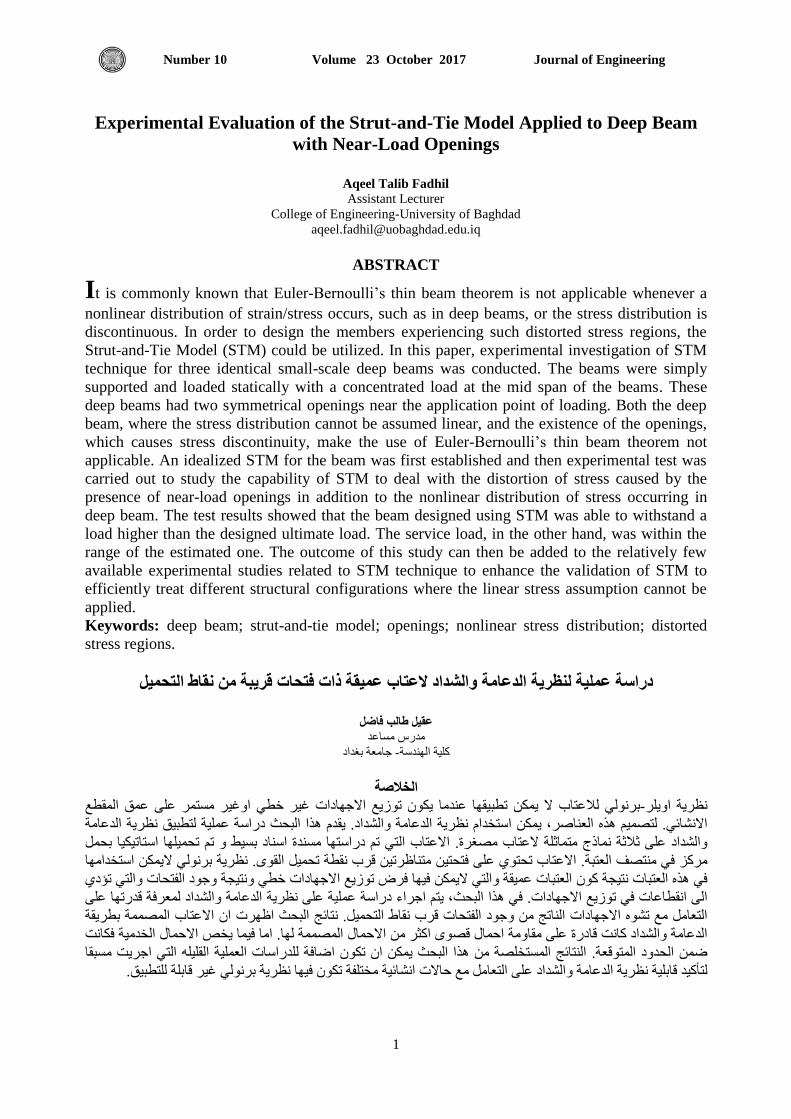
Experimental Evaluation of the Strut-and-Tie Model Applied to Deep Beam
with Near-Load Openings
Aqeel Talib Fadhil
Assistant Lecturer
College of Engineering-University of Baghdad
ABSTRACT
It is commonly known that Euler-Bernoulli’s thin beam theorem is not applicable whenever a
nonlinear distribution of strain/stress occurs, such as in deep beams, or the stress distribution is
discontinuous. In order to design the members experiencing such distorted stress regions, the
Strut-and-Tie Model (STM) could be utilized. In this paper, experimental investigation of STM
technique for three identical small-scale deep beams was conducted. The beams were simply
supported and loaded statically with a concentrated load at the mid span of the beams. These
deep beams had two symmetrical openings near the application point of loading. Both the deep
beam, where the stress distribution cannot be assumed linear, and the existence of the openings,
which causes stress discontinuity, make the use of Euler-Bernoulli’s thin beam theorem not
applicable. An idealized STM for the beam was first established and then experimental test was
carried out to study the capability of STM to deal with the distortion of stress caused by the
presence of near-load openings in addition to the nonlinear distribution of stress occurring in
deep beam. The test results showed that the beam designed using STM was able to withstand a
load higher than the designed ultimate load. The service load, in the other hand, was within the
range of the estimated one. The outcome of this study can then be added to the relatively few
available experimental studies related to STM technique to enhance the validation of STM to
efficiently treat different structural configurations where the linear stress assumption cannot be
applied.
Keywords: deep beam; strut-and-tie model; openings; nonlinear stress distribution; distorted
stress regions.
قريبة من نقاط التحميل فتحاتالذعامة والشذاد العتاب عميقة رات دراسة عملية لنظرية
عقيل طالة فاضل
يذسط يساعذ
خايعت بغذاد -كهت انذست
الخالصة
انقطع عق عه يسخش اغش خط غشاالخاداث حصع ك عذيا احطبق ك ال نالعخاب بشن-اهش ظشت
انذعايت ظشت نخطبق عهت دساست انبحث زا قذو .انشذاد انذعايت ظشت اسخخذاو ك, انعاصشز نخصى. االشائ
بحم اسخاحكا ححها حى بسط اساد يسذة خ حى دساسخاان االعخاب. يصغشة العخاب يخاثهت ارج ثالثت عه انشذاد
اسخخذايا الك بشن ظشت. انق ححم قطت قشب يخاظشح فخحخ عه ححخ االعخاب. انعخبت يخصف ف يشكض
حؤد انخ انفخحاث خد خدت خط االخاداث حصع فشض فا الك انخ عقت انعخباث ك دتخ انعخباث ز ف
عه قذسحا نعشفت انشذاد انذعايت ظشت عه عهت دساست اخشاء خى ,انبحث زا ف. االخاداث حصع ف اقطاعاث ان
بطشقت انصت االعخاب ا اظشث انبحث خائح. انخحم قاط قشب انفخحاث خد ي اناحح االخاداث حش يع انخعايم
فكاج انخذيت االحال خص فا ايا. نا انصت االحال ي اكثش قص احال يقايت عه قادسة كاج انشذاد انذعايت
يسبقا اخشج انخ انقهه انعهت نهذساساث اضافت حك ا ك انبحث زا ي انسخخهصت انخائح. انخقعت حذدان ض
.نهخطبق قابهت غش بشن ظشت فا حك يخخهفت اشائت حاالث يع انخعايم عه انشذاد انذعايت ظشت قابهت نخأكذ
Journal of Engineering Volume 23 October 2017 Number 10
2
.تشوه االجهادات, توزيع االجهادات الالخطيعتب عميق, نظرية الدعامة والشداد, فتحات, : رئيسيةلمات الالك
1. INTRODUCTION
Structural members come in a variety of configurations to comply with different structural
demands. It is, therefore, hard to presume a unified assumption that can be applied precisely to
all structural members. Euler-Bernoulli’s thin beam theorem is one of those theories that cannot
be applied to all structural components.
In general, structural elements can be grouped in two categories, Wight and MacGregor 2012,:
B-regions (Beam regions) where the assumptions of Euler-Bernoulli’s thin beam theorem
can be applied including linear stress distribution assumption.
D-regions (Disturbed or Discontinuous regions) where Euler-Bernoulli’s thin beam
theory cannot be used.
Strut-and–tie modeling approach is considered a valuable technique to design D-regions or
nonlinear stress regions including deep beams. The strut-and–tie model was first introduced in
the ACI 318-02 code, 2002, in 2002 as an appendix. After that, it has been included within the
code context as a main chapter including the latest ACI code 318-14, 2014. The strut-and-tie
model is a simple method that is basically derived from the truss analogy. The idea is to draw the
flow of forces inside the structural member as struts and ties. The force in struts is resisted by
concrete while reinforcement is designed and placed to resist the tension in ties. Several patterns
of load paths may be constructed for the same loading conditions provided that the truss pattern
and components satisfy the recommendations specified by the ACI code, as it is the reference
code for this study, or the provisions specified by other codes of practice.
ACI 318-14 code, 2014, defines the beam as a deep beam if a concentrated load acts within a
distance less than twice the depth of the beam, or if the clear span between the beam’s supports
is less than fourth times the depth of the beam. Once the beam is identified as a deep beam, ACI
318-14 code, 2014, recommends two methods to design the beam; either by taking into
consideration the nonlinear distribution of the strains, without mentioning further details, or by
using the strut-and-tie model.
One of the earliest and pioneering studies to address the design of deep beams with web
openings was carried out by Kong and Sharp, 1977. The study continued earlier pilot tests that
had also been conducted by Kong and Sharp, 1973, which focused on “Shear strength of
lightweight reinforced concrete deep beams with web openings.” The total beams tested in both
studies were 56 deep beams with various beam and opening dimensions and different openings
locations. At that time, no regulations within the codes of practice covered the design of deep
beam with web opening. The researchers implicitly used the basics of the strut-and-tie model for
the design. The final outcome made by Kong and Sharp, 1977, was a modified shear strength
formula and hints for the design of similar cases.
Following Kong and sharp several researches addressed the design of deep beams with web
openings aiming to introduce a design method for such cases. Many of these researches used in
some parts the load path method to bypass the existence of openings in the beam. The results of
these assumptions proved that it was a good structural treatment for the presence of openings.
After that, the load path treatment was developed to the strut-and-tie model approach as a simple
yet a powerful design method. Among these researchers are Kong et al., 1978, Kubik, 1980,
Mansur and Alwis, 1984, Haque et al., 1986, and Schlaich et al., 1987.
Several theoretical studies have been introduced later in order to address the use of strut-and-ties
models in different structural members. However, a relatively few experimental verification tests
Journal of Engineering Volume 23 October 2017 Number 10
3
have been made related to the implementation of the strut-and-ties models in various scenarios
including tests carried out by Maxwell and Breen, 2000, Chen et al., 2002, Ley et al., 2007,
Zhang and Tan, 2007, Campione and Minafò, 2011, Arabzadeh et al., 2011, Nagrodzka-
Godycka and Piotrkowski, 2012, He et al., 2012, and Tuchscherer et al., 2014. Good amount
of experimental verifications will support and encourage engineers to better utilize this simple
method in many structural cases where the linear stress beam theory cannot be utilized. It was
noted by reviewing the previous experimental tests that the web opening in most of these studies
were placed relatively away from the loading source and closer to the supports or to the middle
region of the beam. Therefore, it was intended herein to place two openings closer to loading
area of beams tested to show that a good strut-and-tie model design can overcome the high stress
distortions that occur between the loading point and the openings. The intent from this study is to
introduce, test, and verify different untraditional structural problem to help increasing the
number of experimental studies that ensure the capabilities of the strut-and–tie model to treat
variety of structural scenarios.
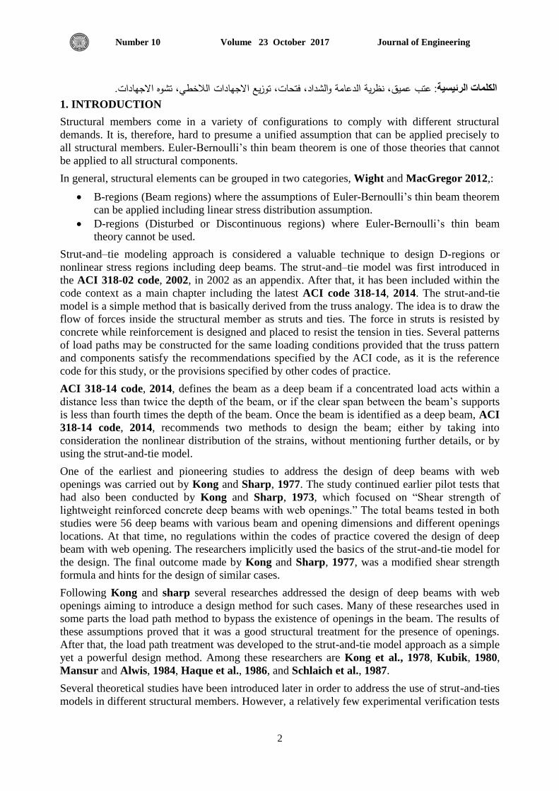
2. SPECIMEN DETAILS
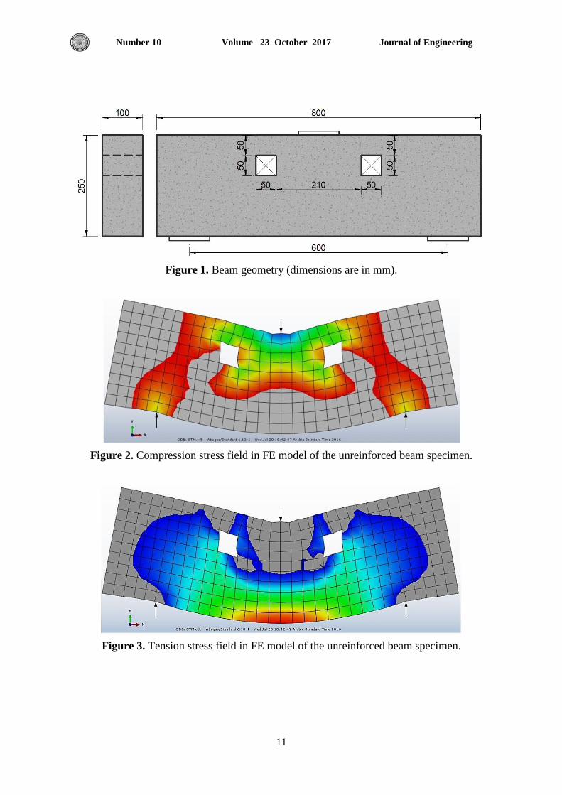
The test involved three identical small-scale deep beam specimens. The geometry of the beam is
shown in Fig. 1. The specimen had a full length of 800mm and a depth of 250mm. The width of
the beam was 100mm. The beam had two symmetrical 50mm by 50mm openings near the
application of the load.
Regarding the size of the openings, there are no available limitations in the current codes of
practice. Many researchers label the openings in their work as "small" or "large" openings
without a clear definition of the size limits between both labels. Mansur M. A., 1998, related
"small" and "large" openings definitions based on the beam response where the large openings
result in Vierendeel action. Beams with large openings require special treatment.
The beam was simply supported with a span length of 600mm center-to-center of the support
which makes the ratio of clear span to overall beam depth equals to 2.0. ACI 318 code, 2014,
classifies the beam as a deep beam if the aforementioned ratio is less than 4. Deep beams can
either be designed by taking into consideration the nonlinearity of strain along the depth or by
using the strut-and-tie model.
Steel bearing plates of 100mm by 100mm were provided at each support to provide the required
bearing width and to simulate the bearing width provided by the columns or supporting girders.
The beam was loaded at the mid span through a steel bearing plate of 100mm by 100mm.
When designed, the beam was intended to carry an ultimate concentrated load of 50kN at the
middle of the beam. This load was supposed to be a combination of factored dead and live load
according to the ACI 318 code, 2014, with load factors equal to 1.2 for the dead load and 1.6 for
the live load. The related service load could then be approximated by dividing the ultimate load
by an average load factor of 1.4 for both dead and live load combined, Maxwell and Breen,
2000, to obtain an equivalent service condition with load factor of 1.0 resulting in a related
service load of 35.71 kN.
3. MATERIAL PROPERTIES
To accommodate the small-scale beam specimen, small reinforcing bar diameters and proper
maximum size of coarse aggregate were adopted. Steel reinforcement and concrete used for this
Journal of Engineering Volume 23 October 2017 Number 10
4
study were tested based on the test methods and procedures recommended by the ASTM
international standards.
Two different reinforcing steel bars were used in this research;
4mm diameter deformed reinforcing bars with cross sectional area of 15.69 mm2, and
6mm diameter deformed reinforcing bars with cross sectional area of 32.15 mm2.
The reinforcing steel used in the study complies with ASTM A615 specifications titled
“Standard Specification for Deformed and Plain Carbon Steel Bars for Concrete
Reinforcement.” The results showed that Ø4mm deformed bars had an average yield strength of
(457 MPa) and an ultimate strength of (606 MPa) while the average yield strength of Ø6mm
deformed bars was (544 MPa) and the ultimate strength was (688 MPa).
Fine and coarse aggregate used in the study complies with ASTM C33 titled “Standard
Specification for Concrete Aggregates” including grading limits for both fine and coarse
aggregate which was conducted in accordance with ASTM C136 “Standard Test Method for
Sieve Analysis of Fine and Coarse Aggregates.”
Mix design was carried out based on the procedure provided by ACI 211.1 titled “Standard
Practice for Selecting Proportions for Normal, Heavyweight, and Mass Concrete” after
gathering the required information from sieve analysis as well as mass densities of fine and
coarse aggregates conducted in accordance with ASTM C127 “Standard Test Method for
Density, Relative Density (Specific Gravity), and Absorption of Coarse Aggregate” and ASTM
C128 “Standard Test Method for Density, Relative Density (Specific Gravity), and Absorption of
Fine Aggregate” The cylinders that were taken at the day of casting the beams were tested
according to ASTM C39 “Standard Test Method for Compressive Strength of Cylindrical
Concrete Specimens” and showed that the concrete had an average specified compressive
strength (fc’) of (29.6 MPa) at the age of 28 days resulting in modulus of elasticity equal to
(25500 MPa) and modulus of rupture equal to (3.3 MPa).
4. STRUT-AND-TIE MODEL DESIGN
4.1 Concept
The design using the strut-and-tie model basically depends on visualizing the stress fields inside
the structural member caused by the applied loads. These stress fields are then illustrated based
on the truss analogy as a combination of struts, for compression stress fields, and ties, for tension
stress fields. Struts and ties are assumed to be connected at nodes to form the complete geometry
of the truss.
Different truss configurations can be drawn for the same loading conditions. The process of the
design using the strut-and-tie model may involve some iterations to select the optimum truss for
the given load. The optimum truss should be able to resist the designed factored load with a
minimal use of reinforcement tie weight which ensures that the selected truss satisfies the
strength requirement as well as the economic considerations. The final truss selected for design
should not only satisfy the strength and economic requirements but also the safety needs
regarding the failure type. In order to prevent brittle failure, a safe design can be accomplished
by attempting to provide a design that allows the beam to deflect to a minimum deflection of
(L/100) at failure, Ley et al., 2007. This ratio is usually considered among the structural
engineers because it is generally thought to be close to the limit of deflection that is noticeable to
the human eye.
Journal of Engineering Volume 23 October 2017 Number 10
5
4.2 Finite Element Implementatıon
As advised by Schlaich et al., 1987, finite elements model can be utilized to get a better
understanding of the stress fields inside the unreinforced structural member. It has not been an
obligation for the researchers to implement the use of finite element when designing using the
strut-and-tie model as it is supposed to be an optional tool for a better design.
For this study, a two-dimensional finite element modeling was performed for the unreinforced
specimen in order to get a better picture about the compression and tension field stresses in the
beam which, in turns, could help configuring the outline of the truss. The two-dimensional finite
element modeling was carried out using Abaqus FEA software.
Since it is a 2D FE Analysis, the element CPS4R was chosen to model the beam. CPS4R element
is a 4-node bilinear plane stress quadrilateral, reduced integration, hourglass control,
Abaqus/CAE, 2011. The beam was sketched with dimensions equal to 800mm in length and
250mm in depth. Two openings were drawn with dimensions of 50mm by 50mm and placed in
its designated position in the tested beam shown in Fig. 1. As it is recommended by Schlaich et
al., 1987, to model the unreinforced beam in the FE model to view the stress path in the concrete
without the help of reinforcement, the only material that was fed to the program is concrete
properties with a mass density of (2400 kg/m3), Young’s Modulus of (25500 MPa) and Poisson’s
Ratio of (0.15). A concentrated load was applied at the middle of the beam to simulate the
loading case at the testing. The output of the major ranges of compression stress field and tension
stress field are shown in Figs. 2 and 3.
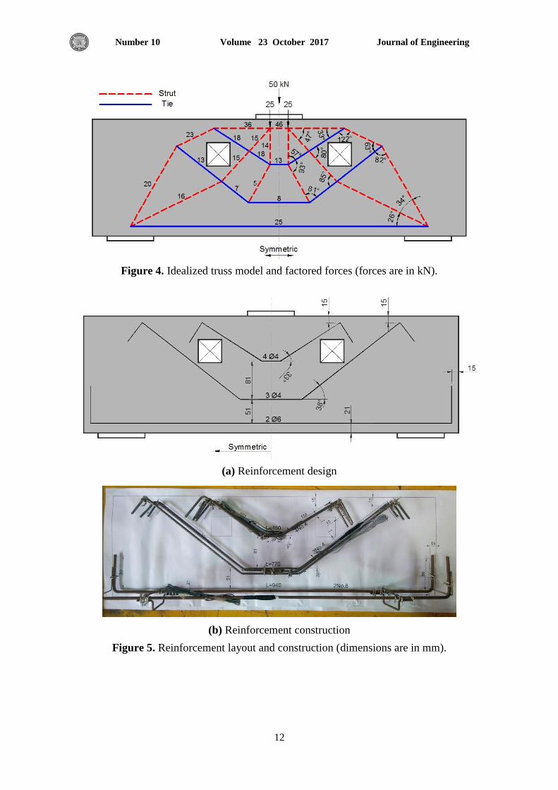
4.3 Idealızed Truss Model
After an extensive study and several iterations of different truss configurations, the idealized
truss shown in Fig. 4 was adopted. The selected truss complies with recommendations of the
ACI 318 code, 2014, found in Chapter 23 which is titled “The Strut-and-Tie Models.”
The limitation of the ACI 318 code, 2014, of providing a minimum angle of (25˚) between any
strut and tie connecting at a single node was considered when designing the idealized truss
layout. Also, the strengths of the ties, struts, and nodal zones of the idealized truss were checked
to satisfy the following ACI criteria, ACI 318 code, 2014.
( ) ( )
( ) ( )
( ) ( )
where Fns, Fnt, and Fnn represent the nominal strength of struts, ties, and at nodal zones
respectively while Fus and Fut represent the factored compressive force in struts and tensile force
in ties respectively. The strength reduction factor (ϕ) equals to 0.75 as specified in the ACI 318
code, 2014.
The factored forces in each strut and tie were calculated after performing the analysis on the
idealized truss as shown in Fig. 4. The nominal strengths of each strut, tie and node were
calculated based on the criteria detailed in the ACI 318 code, 2014. For each member of the
truss, the inequalities of Eqs. (1) - (3) were checked and; hence, the designed truss should be able
to transfer the concentrated load thought the truss to the supports.
Journal of Engineering Volume 23 October 2017 Number 10
6
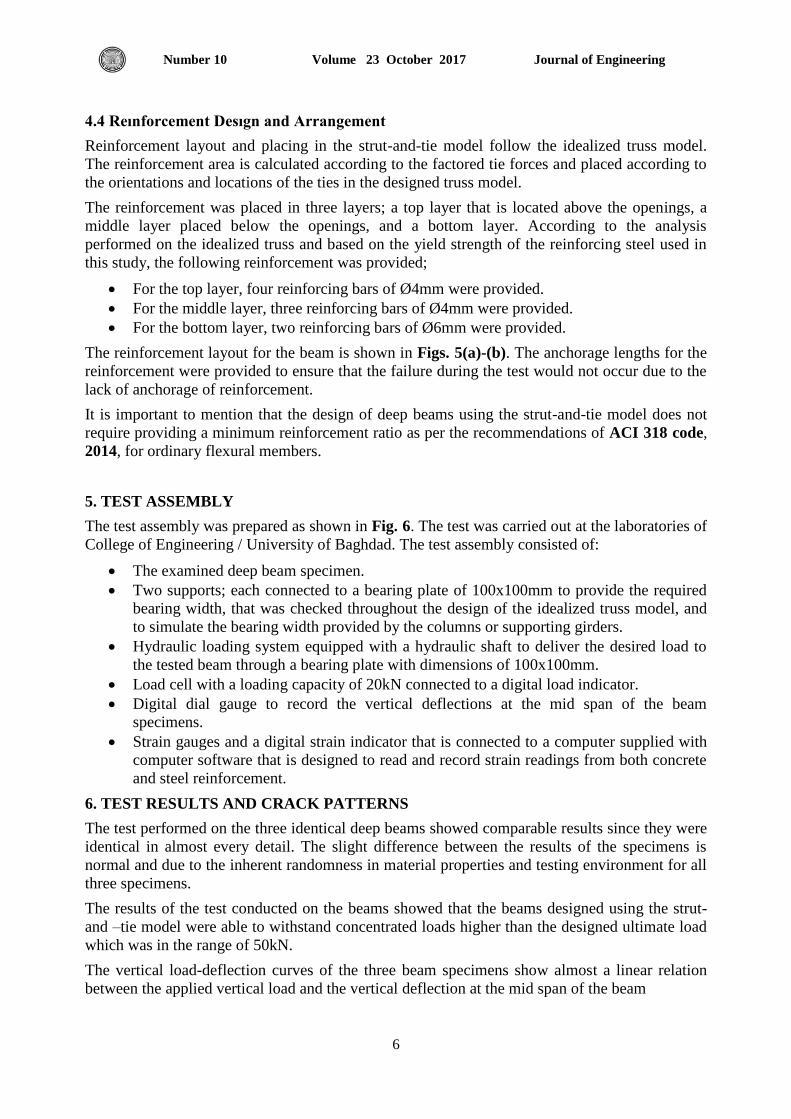
4.4 Reınforcement Desıgn and Arrangement
Reinforcement layout and placing in the strut-and-tie model follow the idealized truss model.
The reinforcement area is calculated according to the factored tie forces and placed according to
the orientations and locations of the ties in the designed truss model.
The reinforcement was placed in three layers; a top layer that is located above the openings, a
middle layer placed below the openings, and a bottom layer. According to the analysis
performed on the idealized truss and based on the yield strength of the reinforcing steel used in
this study, the following reinforcement was provided;
For the top layer, four reinforcing bars of Ø4mm were provided.
For the middle layer, three reinforcing bars of Ø4mm were provided.
For the bottom layer, two reinforcing bars of Ø6mm were provided.
The reinforcement layout for the beam is shown in Figs. 5(a)-(b). The anchorage lengths for the
reinforcement were provided to ensure that the failure during the test would not occur due to the
lack of anchorage of reinforcement.
It is important to mention that the design of deep beams using the strut-and-tie model does not
require providing a minimum reinforcement ratio as per the recommendations of ACI 318 code,
2014, for ordinary flexural members.
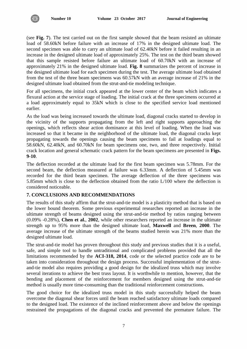
5. TEST ASSEMBLY
The test assembly was prepared as shown in Fig. 6. The test was carried out at the laboratories of
College of Engineering / University of Baghdad. The test assembly consisted of:
The examined deep beam specimen.
Two supports; each connected to a bearing plate of 100x100mm to provide the required
bearing width, that was checked throughout the design of the idealized truss model, and
to simulate the bearing width provided by the columns or supporting girders.
Hydraulic loading system equipped with a hydraulic shaft to deliver the desired load to
the tested beam through a bearing plate with dimensions of 100x100mm.
Load cell with a loading capacity of 20kN connected to a digital load indicator.
Digital dial gauge to record the vertical deflections at the mid span of the beam
specimens.
Strain gauges and a digital strain indicator that is connected to a computer supplied with
computer software that is designed to read and record strain readings from both concrete
and steel reinforcement.
6. TEST RESULTS AND CRACK PATTERNS
The test performed on the three identical deep beams showed comparable results since they were
identical in almost every detail. The slight difference between the results of the specimens is
normal and due to the inherent randomness in material properties and testing environment for all
three specimens.
The results of the test conducted on the beams showed that the beams designed using the strut-
and –tie model were able to withstand concentrated loads higher than the designed ultimate load
which was in the range of 50kN.
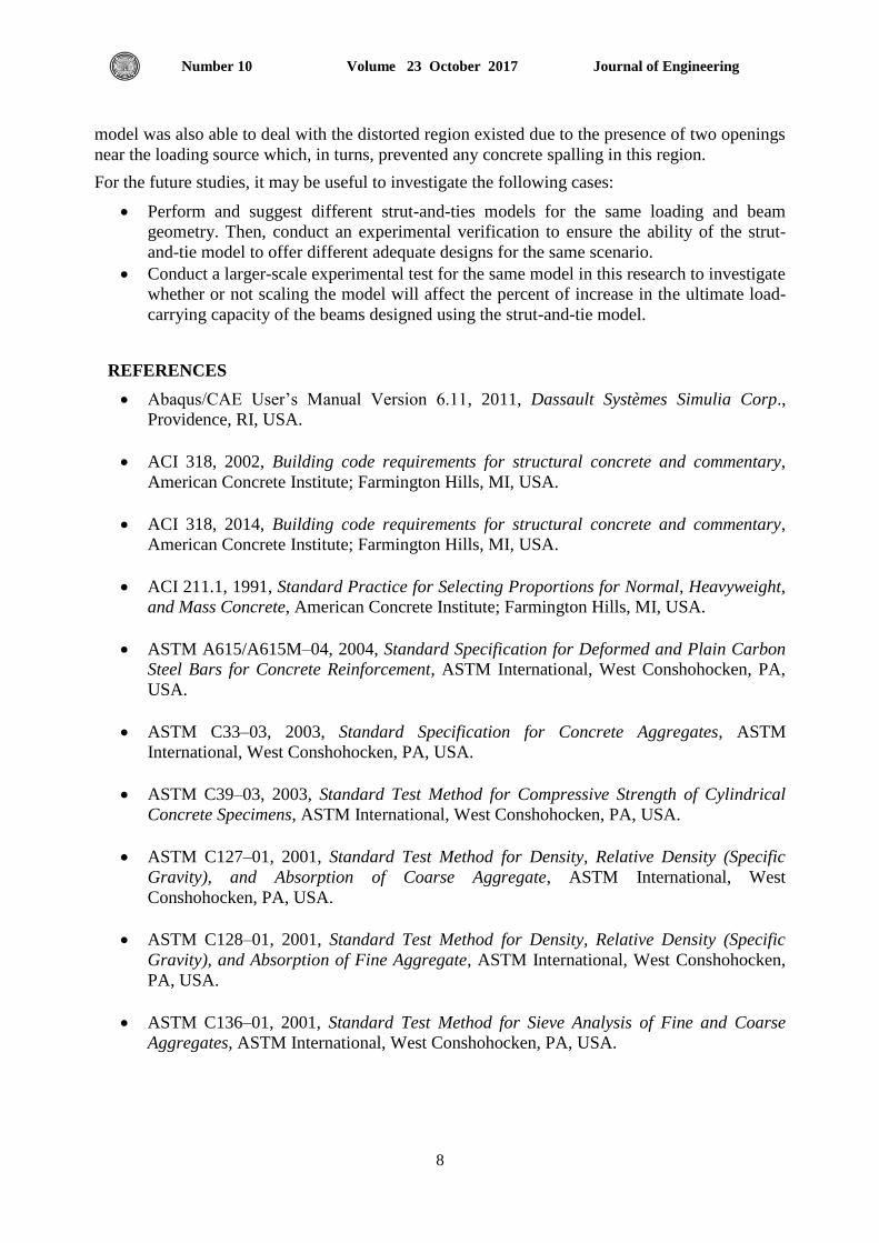
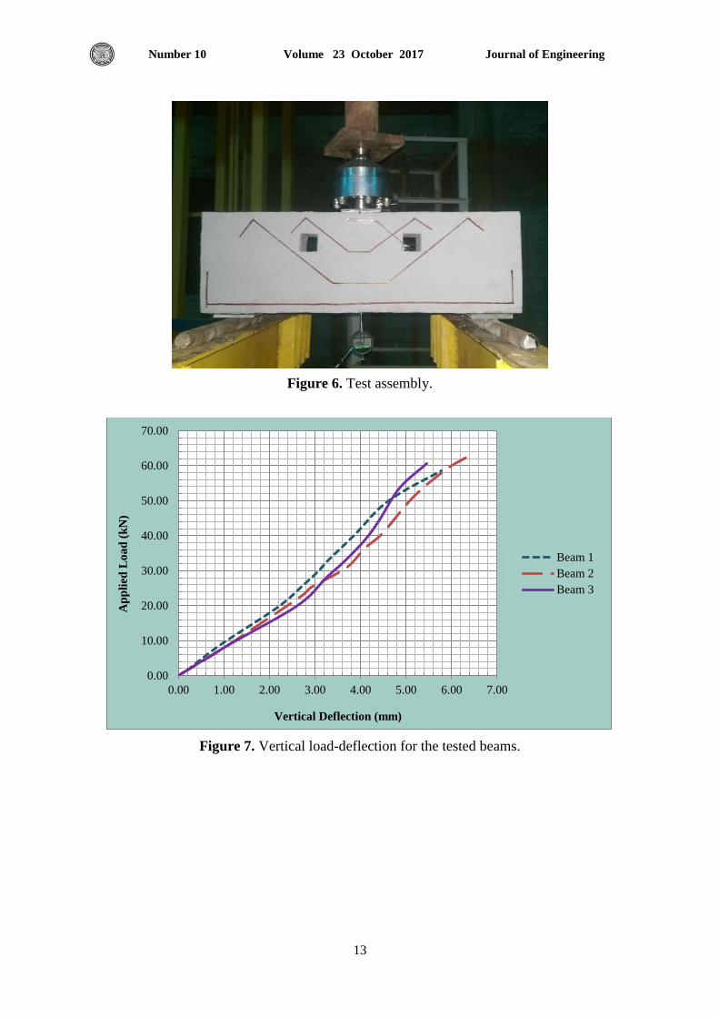
The vertical load-deflection curves of the three beam specimens show almost a linear relation
between the applied vertical load and the vertical deflection at the mid span of the beam
Journal of Engineering Volume 23 October 2017 Number 10
7
(see Fig. 7). The test carried out on the first sample showed that the beam resisted an ultimate
load of 58.60kN before failure with an increase of 17% in the designed ultimate load. The
second specimen was able to carry an ultimate load of 62.40kN before it failed resulting in an
increase in the designed ultimate load of approximately 25%. The test on the third beam showed
that this sample resisted before failure an ultimate load of 60.70kN with an increase of
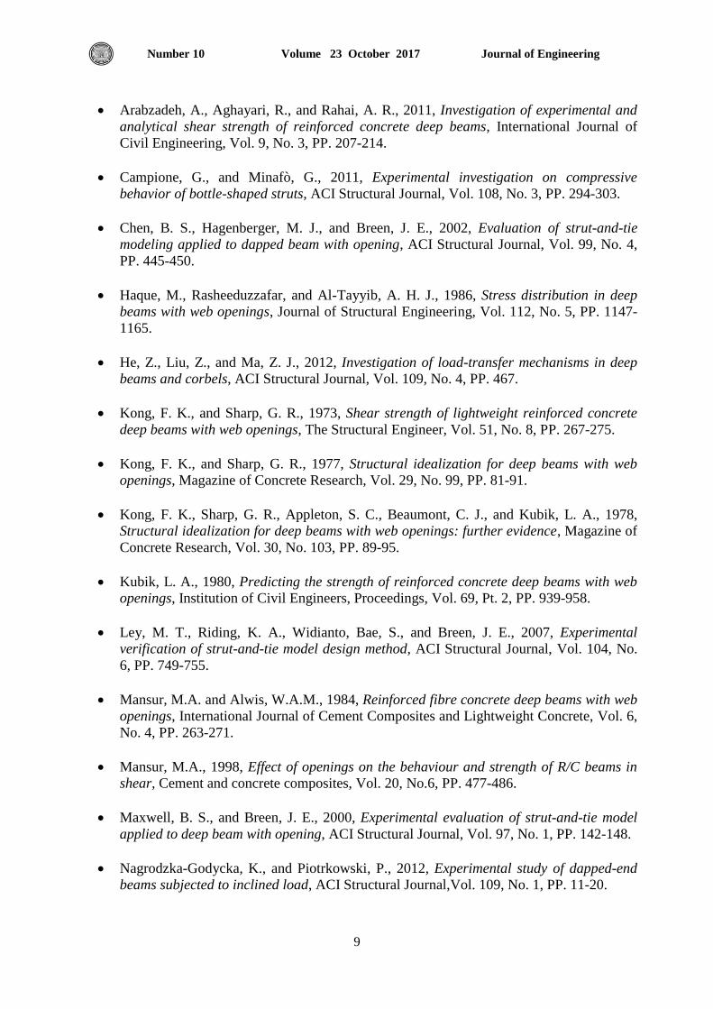
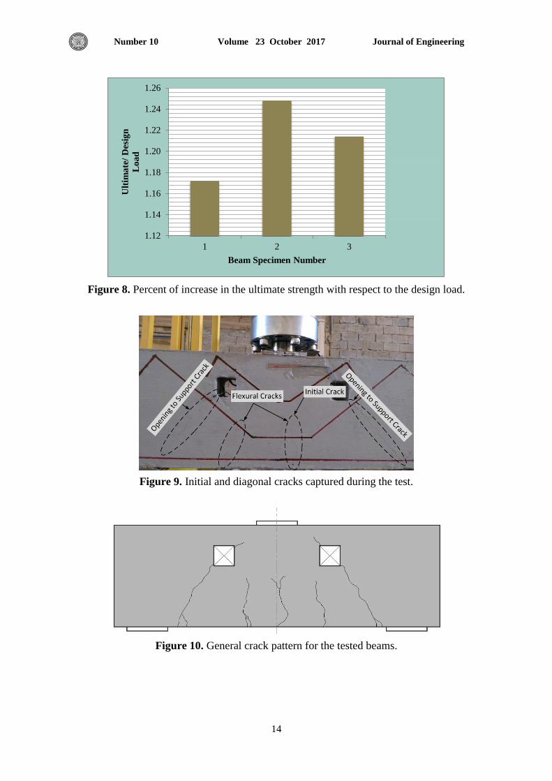
approximately 21% in the designed ultimate load. Fig. 8 summarizes the percent of increase in
the designed ultimate load for each specimen during the test. The average ultimate load obtained
from the test of the three beam specimens was 60.57kN with an average increase of 21% in the
designed ultimate load obtained from the strut-and-tie modeling technique.
For all specimens, the initial crack appeared at the lower center of the beam which indicates a
flexural action at the service stage of loading. The initial crack at the three specimens occurred at
a load approximately equal to 35kN which is close to the specified service load mentioned
earlier.
As the load was being increased towards the ultimate load, diagonal cracks started to develop in
the vicinity of the supports propagating from the left and right supports approaching the
openings, which reflects shear action dominance at this level of loading. When the load was
increased so that it became in the neighborhood of the ultimate load, the diagonal cracks kept
propagating towards the openings causing the beam specimens to fail at loadings equal to
58.60kN, 62.40kN, and 60.70kN for beam specimens one, two, and three respectively. Initial
crack location and general schematic crack pattern for the beam specimens are presented in Figs.
9-10.
The deflection recorded at the ultimate load for the first beam specimen was 5.78mm. For the
second beam, the deflection measured at failure was 6.33mm. A deflection of 5.45mm was
recorded for the third beam specimen. The average deflection of the three specimens was
5.85mm which is close to the deflection obtained from the ratio L/100 where the deflection is
considered noticeable.
7. CONCLUSIONS AND RECOMMENDATIONS
The results of this study affirm that the strut-and-tie model is a plasticity method that is based on
the lower bound theorem. Some previous experimental researches reported an increase in the
ultimate strength of beams designed using the strut-and-tie method by ratios ranging between
(0.09% -0.28%), Chen et al., 2002, while other researchers reported an increase in the ultimate
strength up to 95% more than the designed ultimate load, Maxwell and Breen, 2000. The
average increase of the ultimate strength of the beams studied herein was 21% more than the
designed ultimate load.
The strut-and-tie model has proven throughout this study and previous studies that it is a useful,
safe, and simple tool to handle untraditional and complicated problems provided that all the
limitations recommended by the ACI-318, 2014, code or the selected practice code are to be
taken into consideration throughout the design process. Successful implementation of the strut-
and-tie model also requires providing a good design for the idealized truss which may involve
several iterations to achieve the best truss layout. It is worthwhile to mention, however, that the
bending and placement of the reinforcement for members designed using the strut-and-tie
method is usually more time-consuming than the traditional reinforcement constructions.
The good choice for the idealized truss model in this study successfully helped the beam
overcome the diagonal shear forces until the beam reached satisfactory ultimate loads compared
to the designed load. The existence of the inclined reinforcement above and below the openings
restrained the propagations of the diagonal cracks and prevented the premature failure. The
Journal of Engineering Volume 23 October 2017 Number 10
8
model was also able to deal with the distorted region existed due to the presence of two openings
near the loading source which, in turns, prevented any concrete spalling in this region.
For the future studies, it may be useful to investigate the following cases:
Perform and suggest different strut-and-ties models for the same loading and beam
geometry. Then, conduct an experimental verification to ensure the ability of the strut-
and-tie model to offer different adequate designs for the same scenario.
Conduct a larger-scale experimental test for the same model in this research to investigate
whether or not scaling the model will affect the percent of increase in the ultimate load-
carrying capacity of the beams designed using the strut-and-tie model.
REFERENCES
Abaqus/CAE User’s Manual Version 6.11, 2011, Dassault Systèmes Simulia Corp.,
Providence, RI, USA.
ACI 318, 2002, Building code requirements for structural concrete and commentary,
American Concrete Institute; Farmington Hills, MI, USA.
ACI 318, 2014, Building code requirements for structural concrete and commentary,
American Concrete Institute; Farmington Hills, MI, USA.
ACI 211.1, 1991, Standard Practice for Selecting Proportions for Normal, Heavyweight,
and Mass Concrete, American Concrete Institute; Farmington Hills, MI, USA.
ASTM A615/A615M–04, 2004, Standard Specification for Deformed and Plain Carbon
Steel Bars for Concrete Reinforcement, ASTM International, West Conshohocken, PA,
USA.
ASTM C33–03, 2003, Standard Specification for Concrete Aggregates, ASTM
International, West Conshohocken, PA, USA.
ASTM C39–03, 2003, Standard Test Method for Compressive Strength of Cylindrical
Concrete Specimens, ASTM International, West Conshohocken, PA, USA.
ASTM C127–01, 2001, Standard Test Method for Density, Relative Density (Specific
Gravity), and Absorption of Coarse Aggregate, ASTM International, West
Conshohocken, PA, USA.
ASTM C128–01, 2001, Standard Test Method for Density, Relative Density (Specific
Gravity), and Absorption of Fine Aggregate, ASTM International, West Conshohocken,
PA, USA.
ASTM C136–01, 2001, Standard Test Method for Sieve Analysis of Fine and Coarse
Aggregates, ASTM International, West Conshohocken, PA, USA.
Journal of Engineering Volume 23 October 2017 Number 10
9
Arabzadeh, A., Aghayari, R., and Rahai, A. R., 2011, Investigation of experimental and
analytical shear strength of reinforced concrete deep beams, International Journal of
Civil Engineering, Vol. 9, No. 3, PP. 207-214.
Campione, G., and Minafò, G., 2011, Experimental investigation on compressive
behavior of bottle-shaped struts, ACI Structural Journal, Vol. 108, No. 3, PP. 294-303.
Chen, B. S., Hagenberger, M. J., and Breen, J. E., 2002, Evaluation of strut-and-tie
modeling applied to dapped beam with opening, ACI Structural Journal, Vol. 99, No. 4,
PP. 445-450.
Haque, M., Rasheeduzzafar, and Al-Tayyib, A. H. J., 1986, Stress distribution in deep
beams with web openings, Journal of Structural Engineering, Vol. 112, No. 5, PP. 1147-
1165.
He, Z., Liu, Z., and Ma, Z. J., 2012, Investigation of load-transfer mechanisms in deep
beams and corbels, ACI Structural Journal, Vol. 109, No. 4, PP. 467.
Kong, F. K., and Sharp, G. R., 1973, Shear strength of lightweight reinforced concrete
deep beams with web openings, The Structural Engineer, Vol. 51, No. 8, PP. 267-275.
Kong, F. K., and Sharp, G. R., 1977, Structural idealization for deep beams with web
openings, Magazine of Concrete Research, Vol. 29, No. 99, PP. 81-91.
Kong, F. K., Sharp, G. R., Appleton, S. C., Beaumont, C. J., and Kubik, L. A., 1978,
Structural idealization for deep beams with web openings: further evidence, Magazine of
Concrete Research, Vol. 30, No. 103, PP. 89-95.
Kubik, L. A., 1980, Predicting the strength of reinforced concrete deep beams with web
openings, Institution of Civil Engineers, Proceedings, Vol. 69, Pt. 2, PP. 939-958.
Ley, M. T., Riding, K. A., Widianto, Bae, S., and Breen, J. E., 2007, Experimental
verification of strut-and-tie model design method, ACI Structural Journal, Vol. 104, No.
6, PP. 749-755.
Mansur, M.A. and Alwis, W.A.M., 1984, Reinforced fibre concrete deep beams with web
openings, International Journal of Cement Composites and Lightweight Concrete, Vol. 6,
No. 4, PP. 263-271.
Mansur, M.A., 1998, Effect of openings on the behaviour and strength of R/C beams in
shear, Cement and concrete composites, Vol. 20, No.6, PP. 477-486.
Maxwell, B. S., and Breen, J. E., 2000, Experimental evaluation of strut-and-tie model
applied to deep beam with opening, ACI Structural Journal, Vol. 97, No. 1, PP. 142-148.
Nagrodzka-Godycka, K., and Piotrkowski, P., 2012, Experimental study of dapped-end
beams subjected to inclined load, ACI Structural Journal,Vol. 109, No. 1, PP. 11-20.

Journal of Engineering Volume 23 October 2017 Number 10
10
Schlaich, J., Schäfer, K., and Jennewein, M., 1987, Toward a consistent design of
structural concrete, PCI Journal, Vol. 32, No. 3, PP. 74-150.
Tuchscherer, R. G., Birrcher, D. B., Williams, C. S, Deschenes, D. J., and Bayrak, O.,
2014, Evaluation of existing strut-and-tie methods and recommended improvements, ACI
Structural Journal, Vol. 111, No. 6, PP. 1451.
Wight, J.K. and MacGregor, J.G., 2012, Reinforced Concrete Mechanics and Design, 6th
Edition, Pearson Education. Inc., Upper Saddle River. NJ, USA.
Zhang, N., and Tan, K., 2007, Size effect in RC deep beams: Experimental investigation
and STM verification, Engineering Structures, Vol. 29, No. 12, PP. 3241-3254.
Journal of Engineering Volume 23 October 2017 Number 10
11
Figure 1. Beam geometry (dimensions are in mm).
Figure 2. Compression stress field in FE model of the unreinforced beam specimen.
Figure 3. Tension stress field in FE model of the unreinforced beam specimen.
Journal of Engineering Volume 23 October 2017 Number 10
12
Figure 4. Idealized truss model and factored forces (forces are in kN).
(a) Reinforcement design
(b) Reinforcement construction
Figure 5. Reinforcement layout and construction (dimensions are in mm).
Journal of Engineering Volume 23 October 2017 Number 10
13
Figure 6. Test assembly.
Figure 7. Vertical load-deflection for the tested beams.
0.00
10.00
20.00
30.00
40.00
50.00
60.00
70.00
0.00 1.00 2.00 3.00 4.00 5.00 6.00 7.00
Ap
pli
ed L
oa
d (
kN
)
Vertical Deflection (mm)
Beam 1
Beam 2
Beam 3
Journal of Engineering Volume 23 October 2017 Number 10
14
Figure 8. Percent of increase in the ultimate strength with respect to the design load.
Figure 9. Initial and diagonal cracks captured during the test.
Figure 10. General crack pattern for the tested beams.
1.12
1.14
1.16
1.18
1.20
1.22
1.24
1.26
1 2 3
Ult
ima
te/
Des
ign
Lo
ad
Beam Specimen Number
Series1
Journal of Engineering Volume 23 October 2017 Number 10
15
Mismanagement Reasons of the Projects Execution Phase
Dr. Hatem Khaleefah Al-Agele Abdulmajeed Jafar Ali
Assistant Professor Researcher
Engineering College-Baghdad University Engineering College-Baghdad University
[email protected] [email protected]
ABSTRACT
The execution phase of the project is most dangerous and the most drain on the resources
during project life cycle, therefore, its need to monitor and control by specialists to exceeded
obstructions and achieve the project goals. The study aims to detect the actual reasons behind
mismanagement of the execution phase. The study begins with theoretical part, where it deals
with the concepts of project, project selection, project management, and project processes. Field
part consists of three techniques: 1- brainstorming, 2- open interviews with experts and 3-
designed questionnaire (with 49 reason. These reasons result from brainstorming and
interviewing with experts.), in order to find the real reasons behind mismanagement of the
execution phase. The most important reasons which are negatively impact on management of the
execution phase that proven by the study were (Inability of company to meet project
requirements because it's specialized and / or large project, Multiple sources of decision and
overlap in powers, Inadequate planning, Inaccurate estimation of cost, Delayed cash flows by
owners, Poor performance of project manager, inefficient decision making process, and the
Negative impact of people in the project area). Finally, submitting a set of recommendations
which will contribute to overcome the obstructions of successful management of the execution
phase.
Key words: execution phase, project mismanagement, brainstorming.
سوء االدارة في مزحلت تنفيذ المشاريع أسباب
عبذالمجيذ جعفز علي
تاحث اجسرش
جاؼح تغذاد -ميح اىهذسح
الخالصت
دوسج حاج اىششوع, ىزك فه ذحراج اىى خالهذؼرثش شحيح ذفز اىششوع ه اىشحيح االخطش واالمثش اسرضافا ىيىاسد
شاقثح وسطشج دققح قى تها اصحاب االخرصاص اجو ذجاوص اىؼقثاخ وذحقق اهذاف اىششوع. إ اىهذف اىذساسح
ىء اداسج اىششوع ف شحيح اىرفز. تذأ اىثحث تاىذساسح اىظشح وإسرطالع ادتاخ هى ىثحث واجاد االسثاب اىحققح وساء س
-2اىؼصف اىزه, -1اىىضىع. تؼذ رىل تذأخ اىذساسح اىذاح واىر اسرذخ ػيى اسرخذا ثالثح ذقاخ ؼرذج وه:
ذ اسرثاطها اىؼصف اىزه واىقاتالخ غ سثثا 49)حرىي ػيى ذص اسرثا -3اىقاتالخ اىفرىحح غ اىخثشاء, و
السثاب اىراىح اجو إجاد االسثاب اىحققح اىؤدح إىى سىء إداسج اىششوع ف شحيح اىرفز. اثثرد اىذساسح ا ااىخثشاء(
ىنىه اىشاسغ اىرخصصح و/ )ػذ قذسج اىششمح ػيى ذيثح رطيثاخ اىششوعاداسج شحيح اىرفز: ػيى ه االمثش ذأثشا
ذأخش صشف , ػذ دقح ذخ اىنيفح, ضؼف اىرخطط ىيششوع, ذؼذد صادس اىقشاس واىرذاخو ف اىصالحاخ, او اىنثشج
واىرأثش اىسيث ىسنا ضؼف ػيح اذخار اىقشسا,, ضؼف اداء ذش اىششوع, سرحقاخ اىقاوه قثو صاحة اىؼو
شحيح اىرفز.ىداسج اىاجحح االذجاوص ؼشقالخ ف سرسه رىصاخ جىػح اىواخشا ذقذ .طقح اىششوع(
حاتم خليفت العجيلي د. إسرار ساػذ
جاؼح تغذاد -ميح اىهذسح
Journal of Engineering Volume 23 October 2017 Number 10
16
1. INTRODUCTION
After 2003, Iraq has got a high income and this have encouraged the successive governments to
adopt a quick and ambitious programs for reconstruction, either by establish new projects for
public infrastructure or by developing the old facilities which are necessary to grow needs of all
sectors. Unfortunately, there are many problems in reconstruction programs because
improvisatory and unplanned. Therefore, they do not achieve their goals. The selection of an
appropriate project for implementation and provide the necessary financial allocations in
addition to proper management, all of which are required to achieve a success project.
2. CONSTRUCTION PROJECT
Construction projects are complex, time-consuming undertakings. The development of a project
typically consists of several stages requiring a diverse range of specialized services. To some
extent each project is unique-no two jobs are ever exactly the same, Sears, et al., 2008. The construction project goal is to build something. What differentiates the industry of
construction from other industries is that its project is large, built on –site, and generally unique,
Gould, 1997.
The major characteristics of a project are as follows:
1- An established objective.
2- A defined life span with a beginning and an end.
3- Usually, the involvement of several departments and professionals.
4- Typically, doing something that has never been done before.
5- Specific time, cost, and performance requirements, Larson, and Gray, 2011.
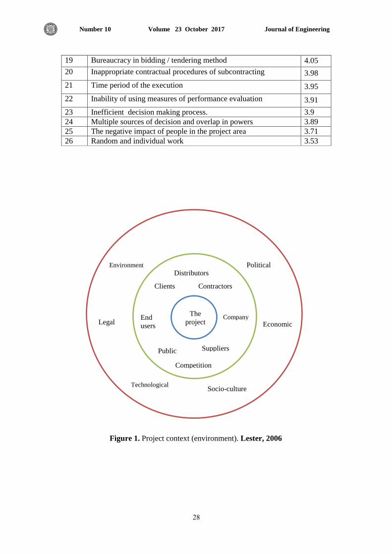
2.1 Project Context (Environment)
Construction project is influenced by multiple factors which can be internal or external to the
organization responsible for its execution and management. The external factors which making
this environment includes the client or customer, contractors, various external consultants,
suppliers, national and local government agencies, competitors, politicians, pressure group,
public utilities, and the end user. Internal influences include the organization's management, the
project team, internal departments, (technical and financial) and possibly the shareholders.
The important thing for the project manager is to recognize what these factors are and how they
impact on the project during the various phases from inception to final handover, or even
disposal, Fig.1 illustrates the project surrounded by its external environment, Lester, 2006.
2.2 Project Selection
The process of projects selection for implementation is subject to several considerations such as;
the needs of organization, realistic expectations for deliverables sophistication, strategic plans,
project success attributes, and the restrictions for the project's success. To make logical and
consistent decisions in prioritizing and projects selection, a company shall establish a specific
process of evaluating projects. Projects ranking is commonly conducted according to certain
criteria and in terms of importance with the use of an index, sometimes called a metric, or a
group of indices called a model. Indices used for project selection tend to fall into two major
categories. The first category includes quantitative indices that are generally based on financial
characteristics such as: total cost, cash flow demand, cost-benefit ratio, Payback period, average
internal rate of return, net present value. The second category includes qualitative indices that are
intended to measure subjective issues, such as operational necessity, competitive necessity,
product line extension, market constraints, Profitability, Feasibility, desirability, recognition, and

Journal of Engineering Volume 23 October 2017 Number 10
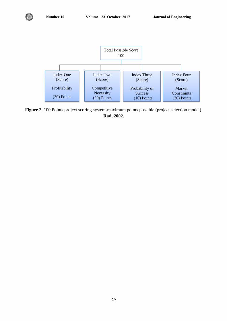
17
success. Fig. 2 shows a simple weighted summation for the results of the of graphical depiction
indices to a selection model that is composed of four indices, Rad, 2002.
2.3 Project Success Criteria One of the topics in the project management plan is the project success criteria. These are the
most important attributes and objectives which must be met to enable the project to be termed a
success. For example if one of the project success criteria is that the project finishes by or before
a certain date, then there can be no compromise of the date, but the cost may increase or quality
may be sacrificed, Lester, 2006.
A project is generally considered to be successfully implemented if it:
a) Comes in on-schedule (time criterion).
b) Comes in on-budget (monetary criterion).
c) Achieves basically all the goals originally set for it (effectiveness criterion).
d) Is accepted and used by the clients for whom the project is intended (client satisfaction
criterion), Pinto, and Slevin, 1987.
2.4 Project Management Is the planning, monitoring and control of all aspects of a project and the motivation of all those
involved in it, in order to achieve the project objectives within agreed criteria of time, cost and
performance. Lester 2006.
2.4.1 Need for project management
It can be summarized the great importance of project management in the following aspects:
a) Project management allows managers to plan and manage strategic initiatives.
b) Project management tools decrease time to market, manage expenses, ensure quality
products, and enhance profitability.
c) Project management helps sell products and services by positively differentiating them
from their competitors.
d) Project management is one of the most important management techniques for ensuring
the success of an organization, Richman, 2011.
2.4.2 Poor project management
The lack of project management by owners or contractors on projects leads to construction
delays and extra costs for both parties. In addition to the problems that occur during
construction, poor project management can also result in a completed facility that fails to meet
the specified quality and suitability of materials, fails to produce the intended products, or
cannot be operated for its intended life. Reasons for project failure that are often cited during
disputes: King, 2015.
1- The failure of the project management team to adequately plan the work, or, when a plan
developed, to properly execute that plan.
2- The failure to provide adequate human resources, staff or direct labor, to the project.
3- The failure to develop adequate project schedules, or to maintain those schedules
throughout project execution.
4- The failure to control costs and changes throughout the execution of the project.

Journal of Engineering Volume 23 October 2017 Number 10
18
3. UNDERSTANDING PROJECT PROCESSES
All projects progress through five project management process groups:
3.1 Initiating Process
The Initiating process determines which projects should be undertaken (project selection). It
examines whether the project is worth doing and if it is beneficial to the company when all is
said and done, PMBOK, 2013.
3.2 Planning Process
The planning process requires establish the scope of the project, refine the objectives, and define
the course of action required to attain the objectives that the project was undertaken to achieve, PMBOK, 2013.
3.3 Executing Process
It is involves the actual "work" of the project. Materials and resources are procured, the project is
produced, and performance capabilities are verified. There are two aspects to the process of
project execution. One is to execute the work that must be done to create the product of the
project. This is properly called technical work. Executing also refers to implementing the project plan, since without a plan there is no control, Heagney, 2012. Executing means carrying out the activities described in the work plan, and where visions and
plans become reality, Dillon, 2008.
3.4 Monitoring and Controlling Process
Monitoring and controlling can actually be thought of as two separate processes, but because
they go hand in hand, they are considered one activity, Heagney, 2012.
Monitoring: Collecting, recording, and reporting information concerning project performance
that project manager and others wish to know.
Controlling: Uses data from monitor activity to bring actual performance to planned
performance, Meredith, and Mantel, 2000.
3.5 Closing Process
Finishing your assigned tasks is only part of bringing your project to a close, Portny, 2010.
If you did a good job of planning and execution, the close-out phase should be fairly simple and
fun. Some project leaders avoid close out because there are unresolved problems with the
project: There are unhappy customers or team members, overrun budgets, and late schedule
dates, Martin, and Tate, 2001.
4. THE TECHNIQUES
The researcher provides detail explanation about the techniques which are used in this part of
the study.
4.1 Brainstorming Technique
It is a creating technique and popular tool of generating ideas to solve a problem. The main
outcome of a brainstorm session may be a full solution to the problem, a set of ideas for an
approach to a subsequent solution, or a set of ideas resulting in a plan to find a solution.
Brainstorming can be used in:
Journal of Engineering Volume 23 October 2017 Number 10
19
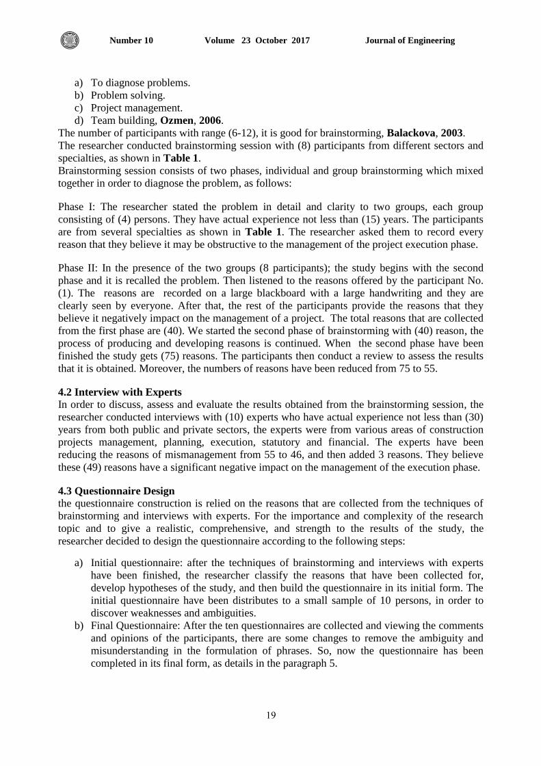
a) To diagnose problems.
b) Problem solving.
c) Project management.
d) Team building, Ozmen, 2006. The number of participants with range (6-12), it is good for brainstorming, Balackova, 2003.
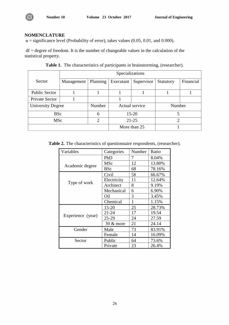
The researcher conducted brainstorming session with (8) participants from different sectors and
specialties, as shown in Table 1.
Brainstorming session consists of two phases, individual and group brainstorming which mixed
together in order to diagnose the problem, as follows:
Phase I: The researcher stated the problem in detail and clarity to two groups, each group
consisting of (4) persons. They have actual experience not less than (15) years. The participants
are from several specialties as shown in Table 1. The researcher asked them to record every
reason that they believe it may be obstructive to the management of the project execution phase.
Phase II: In the presence of the two groups (8 participants); the study begins with the second
phase and it is recalled the problem. Then listened to the reasons offered by the participant No.
(1). The reasons are recorded on a large blackboard with a large handwriting and they are
clearly seen by everyone. After that, the rest of the participants provide the reasons that they
believe it negatively impact on the management of a project. The total reasons that are collected
from the first phase are (40). We started the second phase of brainstorming with (40) reason, the
process of producing and developing reasons is continued. When the second phase have been
finished the study gets (75) reasons. The participants then conduct a review to assess the results
that it is obtained. Moreover, the numbers of reasons have been reduced from 75 to 55.
4.2 Interview with Experts
In order to discuss, assess and evaluate the results obtained from the brainstorming session, the
researcher conducted interviews with (10) experts who have actual experience not less than (30)
years from both public and private sectors, the experts were from various areas of construction
projects management, planning, execution, statutory and financial. The experts have been
reducing the reasons of mismanagement from 55 to 46, and then added 3 reasons. They believe
these (49) reasons have a significant negative impact on the management of the execution phase.
4.3 Questionnaire Design
the questionnaire construction is relied on the reasons that are collected from the techniques of
brainstorming and interviews with experts. For the importance and complexity of the research
topic and to give a realistic, comprehensive, and strength to the results of the study, the
researcher decided to design the questionnaire according to the following steps:
a) Initial questionnaire: after the techniques of brainstorming and interviews with experts
have been finished, the researcher classify the reasons that have been collected for,
develop hypotheses of the study, and then build the questionnaire in its initial form. The
initial questionnaire have been distributes to a small sample of 10 persons, in order to
discover weaknesses and ambiguities.
b) Final Questionnaire: After the ten questionnaires are collected and viewing the comments
and opinions of the participants, there are some changes to remove the ambiguity and
misunderstanding in the formulation of phrases. So, now the questionnaire has been
completed in its final form, as details in the paragraph 5.
Journal of Engineering Volume 23 October 2017 Number 10
20
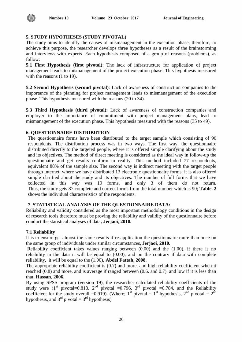
5. STUDY HYPOTHESES (STUDY PIVOTAL)
The study aims to identify the causes of mismanagement in the execution phase; therefore, to
achieve this purpose, the researcher develops three hypotheses as a result of the brainstorming
and interviews with experts. Each hypothesis composed of a group of reasons (problems), as
follow:
5.1 First Hypothesis (first pivotal): The lack of infrastructure for application of project
management leads to mismanagement of the project execution phase. This hypothesis measured
with the reasons (1 to 19).
5.2 Second Hypothesis (second pivotal): Lack of awareness of construction companies to the
importance of the planning for project management leads to mismanagement of the execution
phase. This hypothesis measured with the reasons (20 to 34).
5.3 Third Hypothesis (third pivotal): Lack of awareness of construction companies and
employer to the importance of commitment with project management plans, lead to
mismanagement of the execution phase. This hypothesis measured with the reasons (35 to 49).
6. QUESTIONNAIRE DISTRIBUTION
The questionnaire forms have been distributed to the target sample which consisting of 90
respondents. The distribution process was in two ways. The first way, the questionnaire
distributed directly to the targeted people, where it is offered simple clarifying about the study
and its objectives. The method of direct meeting is considered as the ideal way in follow-up the
questionnaire and get results conform to reality. This method included 77 respondents,
equivalent 88% of the sample size. The second way is indirect meeting with the target people
through internet, where we have distributed 13 electronic questionnaire forms, it is also offered
simple clarified about the study and its objectives. The number of full forms that we have
collected in this way was 10 forms, and only 3 of them do not return.
Thus, the study gets 87 complete and correct forms from the total number which is 90; Table. 2
shows the individual characteristics of the respondents.
7. STATISTICAL ANALYSIS OF THE QUESTIONNAIRE DATA:
Reliability and validity considered as the most important methodology conditions in the design
of research tools therefore must be proving the reliability and validity of the questionnaire before
conduct the statistical analyses of data, Jerjaoi, 2010.
7.1 Reliability
It is to ensure get almost the same results if re-application the questionnaire more than once on
the same group of individuals under similar circumstances, Jerjaoi, 2010.
Reliability coefficient takes values ranging between (0.00) and the (1.00), if there is no
reliability in the data it will be equal to (0.00), and on the contrary if data with complete
reliability, it will be equal to the (1.00), Abdel Fattah, 2008. The appropriate reliability coefficient is (0.7) and more, and high reliability coefficient when it
reached (0.8) and more, and is average if ranged between (0.6. and 0.7), and low if it is less than
that, Hassan, 2006.
By using SPSS program (version 19), the researcher calculated reliability coefficients of the
study were (1st pivotal=0.813, 2
nd pivotal =0.796, 3
rd pivotal =0.784, and the Reliability
coefficient for the study overall =0.919). (Where; 1st pivotal = 1
st hypothesis, 2
nd pivotal = 2
nd
hypothesis, and 3rd
pivotal = 3rd
hypothesis)
Journal of Engineering Volume 23 October 2017 Number 10
21
7.2 Validity It is the degree to which a questionnaire reflects reality. The researcher calculates the validity
coefficient from calculating the root of reliability coefficient, Abdel Fattah, 2008.
Validity coefficients of the study were (1st pivotal =0.902, 2
nd pivotal =0.892, 3
rd pivotal =0.885,
and the Validity coefficient of the study overall =0.959).
Aarbitrators validity is one of the most common and easy methods of validity and the best
known among researchers, Jerjaoi, 2010. As ti ti mentioned earlier, the questionnaire is designed in consulting with ten experts; therefore,
we also won the validity of arbitrators
7.3 Test of Normality Applied researchers should always look at the shape of their data before conducting statistical
tests. Looking at data can give you some idea about whether your data are normality distributed,
Larson-Hall, 2010. The researcher adopted two tests, Shapiro-wilks and Kolmogorov to test the distribution type of
answers is it normal (equinoctial) or not. These tests are necessary to check the study hypotheses, because most of parametric tests require normal distribution for data, Abu Dakka, and Safi,
2013. By using (assume) a significance level (α = 0.05), we will test the type of answers distribution of
all reasons. In the beginning we assume two hypotheses, the first is the null hypothesis (H0),
and the second is the alternative hypothesis (H1). Null hypothesis means that the distribution of
the sample answers behaves as normal, accepts this hypothesis if the value of significance (sig.
which computed by SPSS program) is greater than (α), and reject if the value of sig. is smaller
than (α).
The alternative hypothesis H1 means that the distribution of the answers is random. This
hypothesis is accepted if the value of computed sig. is smaller than (α) and it is rejected if the
value of computed sig. is greater than value of (α). As it is shown in Table. 3, the sig. values are
computed for the first four reasons were less than of (α=0.05), therefore, the null hypothesis is
rejected and accepts the alternative hypothesis which means that the distribution is random,
Larson-Hall, 2010. The results of normality test for all answers show that the distribution are random.
7.4 Likert Scale
A psychometric response scale mainly used in questionnaires to get participant’s preferences or
degree of agreement with a statement or group of statements. Ask Respondents to indicate their
agreement level with a given statement by using an ordinal scale, Johns, 2010. The design of the questionnaire is based on that the answer of each question is one of five
options. So, the likert scale quintet is used. It is usually enter values (weights) as in the Table. 4.
Abdel Fattah, 2008.
7.5 The Mean It is the algebraic sum of a set of items divided by their number. It uses with quantitative
variables in the case of similar distributions (almost), especially if we take into account all the
values, Larson-Hall, 2010.
By using SPSS program (Version 19), the mean of all reasons are calculate, and then compare
with the weighted mean to know the trend of answers on each reason, whether it is acceptable or
not, or neutral.
Journal of Engineering Volume 23 October 2017 Number 10
22
7.6 Chi-Square
Chi-square: As it is proved in the paragraph “test of normality”, the distributions of respondents'
answers were random. Here, non-parametric tests are used, including chi-square. The chi-square
test is used to examine the presence of statistically significant differences between answers
(approval, neutrality, and disapproval). This test is based on comparison the calculated chi-
square against scheduled chi-square at a significance level (α = 0.05). It is supposed that:
1) The null hypothesis or (H0) stated: (distribution of the respondents answers are regular, and
the differences in those answers can be attributed to chance), this hypothesis is accepted if
calculated chi-square is less than scheduled chi-square and it is rejected if calculated chi-square
is greater than scheduled one.
2) Alternative hypothesis (H1) stated: (distribution of the respondents answers are irregular),
this hypothesis is accepted if the value of calculated chi-square is greater than the value of
scheduled chi-square and it is rejects if calculated chi-square is less than a scheduled one, Bousnina, 2011.
8. RESULTS
After the statistical operations on the data have finished, it is reached the following results:
8.1 First:
After the statistical analysis on the questionnaire data have been finished, the researcher
identified the reasons which have a significant negative impact on the management of project
execution phase, which are (26) reasons; below it is mention some of them:
1- Inability of company to meet project requirements because it's specialized and / or large
project, with agreement ratio reached (4.68).
2- Inefficient and non- professional supervision committees, with agreement ratio 4.66.
3- Inadequate planning, with agreement ratio 4.62.
4- Relying on manager only to control the project, with agreement ratio 4.53.
5- Unrealistic project plan, with agreement ratio 4.51.
6- Inaccurate estimation of cost, with an agreement ratio 4.48.
7- Poor performance of Project Manager, with agreement ratio 4.39.
8- Delayed cash flows by owners, with agreement ratio 4.37.
9- Poor performance of contractor, with agreement ratio 4.14.
10- Inefficient decision making process, with agreement ratio 3.9.
11- Multiple sources of decision and the overlap in powers, with agreement ratio 3.89.
12- Negative impact of people in the project area, with agreement ratio 3.71.
The agreement ratio on each reason is represent the mean value according to Likert scale quintet.
The total (26) reasons which are lead to mismanagement of the execution phase are descendingly
arranged according to value of the mean as it is shown in Table. 5. All reasons that have been
approved by the study have statistically significant differences, since the value of calculated chi
is greater than the scheduled chi.

Journal of Engineering Volume 23 October 2017 Number 10
23
8.2 Second
Prove the hypotheses of the study overall, as follows:
1) Prove the first hypothesis of the study which states that, the lack of infrastructure for
application of project management leads to mismanagement of the execution phase, where the
ratio of those who agree with this hypothesis reached 54.63%, and the chi calculated (513)
greater than chi scheduled (9.488) which indicates the presence of statistically significant
difference between answers.
2) Prove the second hypothesis of the study which states that, lack of awareness of construction
companies to the importance of planning for project management leads to mismanagement of the
execution phase, where the ratio of those who agree with this hypothesis reached 71.34%, and
the chi calculated (615) greater than chi scheduled (9.488) which indicates the presence of
statistically significant difference between answers.
3) Prove the third hypothesis of the study which states that, lack of awareness of construction
companies and employer to the importance of commitment with project management plans leads
to mismanagement of the execution phase, where the ratio of those who agree with this
hypothesis reached 68.28%, and the chi calculated (553) greater than chi scheduled (9.488)
which indicates the presence of statistically significant difference between answers.
9. CONCLUSIONS
The most important conclusions are:
1. The agreement of respondents on hypotheses of the study will imparts realism to the study and
its results, (Ranking: 1- 2nd
hypothesis, 2- 3rd
hypothesis, and 3- 1st hypothesis).
2. The choice of construction project for implementation is subject to improvisational and chaos
with a lack of clear criteria in the selection process.
3. The full absence of vocational rehabilitation centers which increases in loss of skilled workers
in the construction industry.
4. Most contractors have not any managerial skill.
5. Reliance on personal experience only in full control of the project with full absence of
standard tools of performance evaluation.
6. Weakness in the supervision and follow up by employer
7. Inability of company to meet project requirements, because it's specialized and / or large
project, is considered as most important factor that leads to mismanagement of the execution
phase.
8. The failure of execution management can be considered as the problems that are not borne by
one party alone, but due to all parties of the project.
9. Inaccurate estimation of costs is one of mismanagement causes
Journal of Engineering Volume 23 October 2017 Number 10
24
10. RECOMMENDATIONS
The study presents a group of recommendations which may help to eliminate or reduce the
negative impact of the reasons of mismanagement of the project execution phase:
1. Restricted to clauses (2, 11, 14, 15, 42, 44, 47, and 62) of the general conditions for contracts
of civil engineering works. because they can help to overcome the reasons of mismanagement.
2. Activating the role of council of reconstruction in provinces and give it wide powers within
the terms of reference. It must play a major role to follow the basic design of province and
protect it, and to take a consultative role in feasibility studies of the projects and also in prepare
their documents.
3. Communicate with competent international bodies is necessary to train the managerial and
technical leadership according to international standards.
4. Encourage the site meetings because their necessity for all parties to the project.
5. The construction companies must rely on trained professional staff in the fields of planning
and execution, even if the wages are high.
6. The importance of communication between the designers and executants for project's success.
7. Importance of statistical databases of previous projects to the planning process for future
projects.
8. Encourage the staff of project, either in the planning or execution and give them reward and
incentives to induce them to do work efficiently.
9. Punish those who aggress on public property, (especially in project area).
10. Do not let the contractor who does not fit his financial and technical ability with project to
offer the bid for implementation of the work by (list qualified contractors or company selection
criteria).
11. Prepare cost estimation depending on WBS, final drawings and direct market surveys.
REFERENCES
Abdel Fattah, A., 2008, Introduction to Descriptive and Inferential Statistics by using
SPSS.
Abu Dakka, S. A., and Safi, S. K., 2013, Practical Applications by using the (Statistical
Packages for Social Sciences) in Educational and Psychological Research.
Balackova, H., 2003, Brainstorming: a creative problem-solving method, Masaryk
Institute of Advanced Studies, Czech Technical University, Prague, Czech Republic.
Johns, R., 2010, Likert Items and Scales, (University of Strathclyde) SQB Methods Fact
Sheet 1 (March 2010)
Bousnina, M. A., 2011, Study the Delays in Construction Projects Because of the Owner.
Journal of Engineering Volume 23 October 2017 Number 10
25
Dillon, L. B., 2008, Project Implementation, published on (http://www.sswm.info/).
Gould, F. E., 1997, Managing the Construction Process. Estimating, Scheduling, and
Project Control.
Hassan, M. A., 2006, The Psychometric Characteristics of Measurement Tools in
Psychological and Educational Research by using SPSS.
Heagney, J., 2012, Fundamentals of Project Management, Fourth Edition, American
Management Association.
Jerjaoi, Z. A., 2010, The Educational Methodology Rules for the Construction of the
Questionnaire.
King, T. D., 2015, Assessment of Problems Associated with Poor Project Management
Performance, Long International, Inc.
Larson, E. W., and Gray, C. F., 2011, Project Management, the managerial process, fifth
edition, by The McGraw-Hill Companies.
Larson-Hall, J., 2010, A guide to Doing Statistics in second language using SPSS, 1st
Edition, by Taylor and Francis.
Lester, A., 2006, Project Management, planning and control, fifth edition.
Martin, P., and Tate, K., 2001, Getting Started in Project Management, Published by
John Wiley & Sons, Inc.
Meredith, J. R., and Mantel, S. J., 2000, Project Management: A Managerial Approach
4/e, Published by John Wiley & Sons, Inc., Presentation prepared by RTBM Web Group
Copyright © 2000.
Ozmen, H., 2006, Brainstorming, www.brainstorming.co.uk/extra/productservices.html.
Pinto, J. K., and Slevin, D. P., 1987, Critical Success Factors in Effective Project
Implementation.
PMBOK, 2013, A Guide to the Project Management Body of Knowledge.
Portny, S. E., 2010, Project Management for Dummies, 3rd Edition.
Rad, P. F., 2002, Project Estimating and Cost Management.
Richman, L., 2011, Successful Project Management, Third Edition.
Sears, S. K., Sears, G. A., and Clough, R. H., 2008, Construction Project Management. A
Practical Guide to Field Construction Management.
Journal of Engineering Volume 23 October 2017 Number 10
26
NOMENCLATURE
α = significance level (Probability of error), takes values (0.05, 0.01, and 0.000).
df = degree of freedom. It is the number of changeable values in the calculation of the
statistical property.
Table 1. The characteristics of participants in brainstorming, (researcher).
Sector
Specializations
Management Planning Executant Supervisor Statutory Financial
Public Sector 1 1 1 1 1 1
Private Sector 1 1
University Degree Number Actual service Number
BSc 6 15-20 5
MSc 2 21-25 2
More than 25 1
Table 2. The characteristics of questionnaire respondents, (researcher).
Variables Categories Number Ratio
Academic degree
PhD 7 8.04% MSc 12 13.80% BSc 68 78.16%
Type of work
Civil 58 66.67% Electricity 11 12.64% Architect 8 9.19% Mechanical 6 6.90% Oil 3 3.45% Chemical 1 1.15%
Experience (year)
15-20 25 28.73% 21-24 17 19.54 25-29 24 27.59 30 & more 21 24.14
Gender Male 73 83.91% Female 14 16.09%
Sector Public 64 73.6% Private 23 26.4%
Journal of Engineering Volume 23 October 2017 Number 10
27
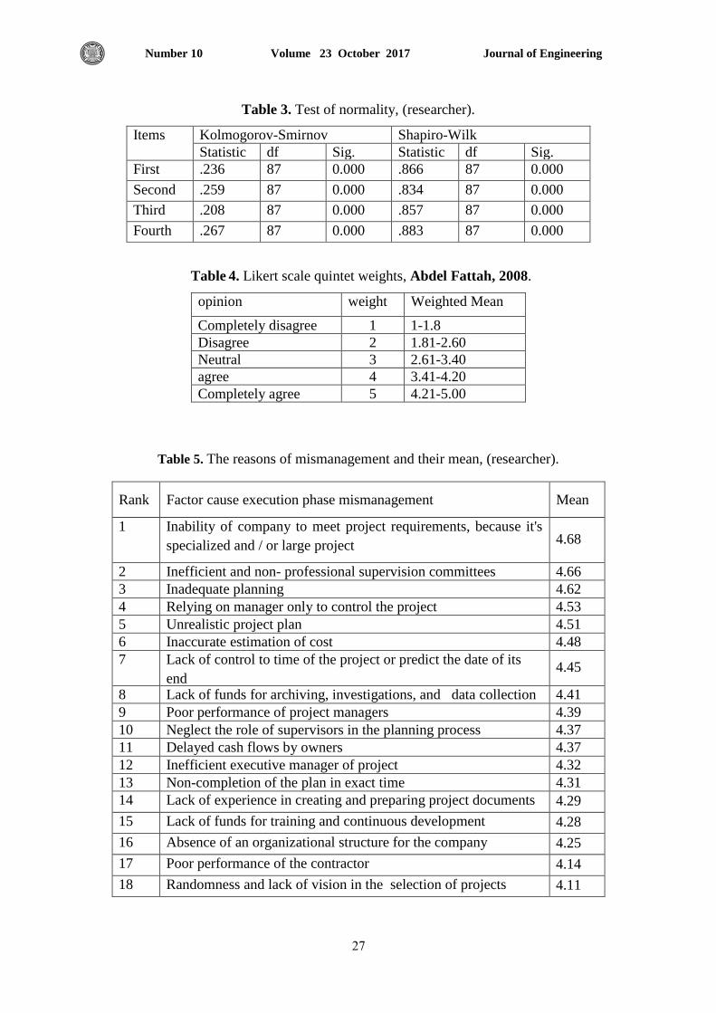
Table 3. Test of normality, (researcher).
Items Kolmogorov-Smirnov Shapiro-Wilk
Statistic df Sig. Statistic df Sig.
First .236 87 0.000 .866 87 0.000
Second .259 87 0.000 .834 87 0.000
Third .208 87 0.000 .857 87 0.000
Fourth .267 87 0.000 .883 87 0.000
Table 4. Likert scale quintet weights, Abdel Fattah, 2008.
opinion weight Weighted Mean
Completely disagree 1 1-1.8
Disagree 2 1.81-2.60
Neutral 3 2.61-3.40
agree 4 3.41-4.20
Completely agree 5 4.21-5.00
Table 5. The reasons of mismanagement and their mean, (researcher).
Rank Factor cause execution phase mismanagement Mean
1 Inability of company to meet project requirements, because it's
specialized and / or large project 4.68
2 Inefficient and non- professional supervision committees 4.66
3 Inadequate planning 4.62
4 Relying on manager only to control the project 4.53
5 Unrealistic project plan 4.51
6 Inaccurate estimation of cost 4.48
7 Lack of control to time of the project or predict the date of its
end 4.45
8 Lack of funds for archiving, investigations, and data collection 4.41
9 Poor performance of project managers 4.39
10 Neglect the role of supervisors in the planning process 4.37
11 Delayed cash flows by owners 4.37
12 Inefficient executive manager of project 4.32
13 Non-completion of the plan in exact time 4.31
14 Lack of experience in creating and preparing project documents 4.29
15 Lack of funds for training and continuous development 4.28
16 Absence of an organizational structure for the company 4.25
17 Poor performance of the contractor 4.14
18 Randomness and lack of vision in the selection of projects 4.11
Journal of Engineering Volume 23 October 2017 Number 10
28
19 Bureaucracy in bidding / tendering method 4.05
20 Inappropriate contractual procedures of subcontracting 3.98
21 Time period of the execution 3.95
22 Inability of using measures of performance evaluation 3.91
23 Inefficient decision making process. 3.9
24 Multiple sources of decision and overlap in powers 3.89
25 The negative impact of people in the project area 3.71
26 Random and individual work 3.53
Figure 1. Project context (environment). Lester, 2006
The
project Legal
Environment Political
Economic
Technological Socio-culture
Distributors
Clients
End
users
Public
Competition
Suppliers
Company
Contractors
Journal of Engineering Volume 23 October 2017 Number 10
29
Figure 2. 100 Points project scoring system-maximum points possible (project selection model).
Rad, 2002.
Total Possible Score
100
Index One
(Score)
Profitability
(30) Points
Index Two
(Score)
Competitive
Necessity
(20) Points
Index Three
(Score)
Probability of
Success
(10) Points
Index Four
(Score)
Market
Constraints
(20) Points
Journal of Engineering Volume 23 October 2017 Number 10
30
Application of Building Information Modeling (3D and 4D) in Construction Sector in Iraq
Kadhim Raheem Erzaij
Assistant Professor
Collage of Engineering-University Of Baghdad E-mail: [email protected]
Ayad Abbas Obaid
MSc student
Collage of Engineering-University Of Baghdad E-mail:[email protected]
ABSTRACT
Building Information Modeling (BIM) is becoming a great known established collaboration
process in Architecture, Engineering, and Construction (AEC) industry. In various cases in
many countries, potential benefits and competitive advantages have been reported. However,
despite the potentials and benefits of BIM technologies, it is not applied in the construction
sector in Iraq just like many other countries of the world.
The purpose of this research is to understand the uses and benefits of BIM for construction
projects in Iraq. This purpose has been done by establishing a framework to application of BIM
and identifying the benefits of this technology that would convince stakeholders for adopting
BIM in the construction sector in Iraq.
Through this research, the use of this technology has been clarified by using the proposed
framework (application Revit software and linking it with the MS Project and Navisworks
Manage software on the case study) to identify the important benefits to be the beginning to
apply the Building Information Modeling technology in the construction sector in Iraq.
The research results indicated that such proposed framework can greatly improve the
performance of the current state of project management through improving the project quality,
cost saving and time-saving.
Keywords: Building information modeling, Architectural Engineering and Construction (AEC)
industry, BIM knowledge, BIM benefits, The construction sector in Iraq.
في العزاق االنشاءفي قطاع (4Dو 3D) تطبيق نمذجة معلومات البناء
اياد عباس عبيذ
طالة ماجسريس
جامعح تغداد-كليح الهندسح
كاظم رحيم ارسيجد.
مساعدسراذ ا
جامعح تغداد-كليح الهندسح
الخالصة
وذشبببييد فببب صبببناعح الر ببب ي ين أعضبببا القسابببل الهندسببب ذعببباو تببب وسبببيلح (BIM) رجبببح معلىمببباخ الثنبببا أصبببثند
فببب عبببدج تلبببدا ف وذببب معسفبببح القىامبببد ال نر لبببح وال لاابببا الرنافسبببيحا ومببب ذلببب وعلببب البببس مبببن م ا يببباخ (AEC) الثنبببا
فببب العبببساك مدبببم العدابببد مبببن الثلبببدا دفببب م ببباا الثنبببا والرشبببيي اوفىامبببد ذ نىلىجيبببا رجبببح معلىمببباخ الثنبببا ف ابببر ذ ثينهببب
األخسيا
الغببسم مببن اببرا الثنبب اببى فهبب اسببرنداماخ وفىامببد رجببح معلىمبباخ الثنببا لل شببازا ا شبباميح فبب العببساكف ومببد ذبب ا
ذلببب الغبببسم مبببن خبببر ا شبببا طببباز ع بببم لر ثيبببل رجبببح معلىمببباخ الثنبببا والرعبببس علببب فىامبببد ابببر الر نىلىجيبببا الرببب
ف العساكا دىماخ الثنا ف م اا الثنا والرشييمن شا ها ا ذنن أصناب ال لنح من اجم اعر اد رجح معل
علببب ةالبببح دزاسبببيح لر بببىان بببىذ ر ببب ا تعببباد (Revit)تس بببام لومبببد ذببب ذىتبببي اسبببرندال ابببر الر نىلىجيبببا تر ثيببب
(ا للرعبببس علببب Navisworks Manage فببب تس بببام (MS Project)ال رىلبببد مبببن وزت بببع مببب اللبببدو اللمنببب
ى تدااح لر ثيل ذ نىلىجيا رجح معلىماخ الثنا ف م اا الثنا والرشييد ف العساكالر ه حالقىامد ال
وأشبببازخ ربببام الثنببب ا طببباز الع بببم ال نربببسر ا بببن ا انسبببن كديبببسا مبببن أدا الىتببب النبببال دازج ال شبببسوا مبببن
خر ذنسين ىعيح ال شسواف ذىفيس الىمد والر اليفا
Journal of Engineering Volume 23 October 2017 Number 10
31
1. INTRODUCTION
1.1 General
The benefits of Building Information Modeling (BIM) are being realized by
construction firms around the world. However, in Iraq it is not applied until now. The
Researcher will explore how the engineers in construction sector can take advantage of
the benefits that BIM allows. BIM is more than just a process; it paves the way to a
new form of project procurement and delivery. To realize the full potential of BIM and
work with the models in the most productive way it needs to have the correct tools and
knowledge.
BIM is a technological system to conveying and storing information for the buildings,
with an ability to visually display buildings parts in a 3-D view. The 3-D capability is
enhanced by the parametric modeling engine, which automatically interrelates building
objects to other objects and coordinates changes and revisions across the project
deliverables, Rundell and Stowe, 2005. For instance, a change to the length of a wall
in a building drawing is automatically reflected in the walls that connect to it. The idea
is that the BIM produces a faster, cheaper, more accurate, and better-coordinated
project experience during design, construction, and future use. With the growth of
information technologies in the field of construction industry over the last years,
numerical building information modeling and process simulation has evolved to a fully
accepted and widely used tool for the project life circle management. Building
information is present through the whole life cycle of the engineering and construction
phases. Due to the long time and the numerous contractors, the phenomena of mass
information and information attenuation occur throughout the life cycle. The traditional
methods of information exchange cannot meet the mass information processing
requirements of modern large-scale construction projects, Ding, L. and X. Xu, 2014.
1.2 Definitions
Due to the different perceptions, overview and experiences of researchers and
professionals in the AEC industry, they can define BIM in different ways
Khosrowshahi and Arayici, 2012. For example, Gu and London, 2010 said that BIM
is an information technology (IT) enabled approach that involves applying and
maintaining an integral digital representation of all building information for different
phases of the project lifecycle in the form of a data repository. On the other hand,
Eastman et al., 2008 emphasized that BIM is not only a tool, but also a process that
allows project team members to have an unprecedented ability to collaborate over the
course of a project, from early design to occupancy. Stebbins, 2009 agreed that BIM is
a process rather than a piece of software. He clearly identified BIM as a business and
management decision. BIM implementation is strongly related to managerial aspects of
professional practices for different working styles and cultures, Ahmad et al., 2012.
BIM has a broad range of applications cross the design; construction; and operation
process ,Baldwin, 2012. BIM is important to develop the design process by managing
the changes in the design. It is efficient in checking and updating all the views (plans,
sections and elevations) when any changes occur, CRC construction innovation,
2007. BIM is a new way of approaching the design and documentation of building
projects.
Journal of Engineering Volume 23 October 2017 Number 10
32
1.3 Objective
The aim of this research is to develop a clear understanding about BIM for identifying
the different factors that provide useful information to consider adopting BIM
technology in projects by practitioners in the construction sector in Iraq. In achieving
this aim, two main objectives have been outlined as follows:
A. To identify the BIM system.
B. To identify the top BIM benefits that would convince professionals for
adopting BIM in the construction sector in Iraq.
2. UNDERSTANDING OF BIM CONCEPT
BIM has been in use internationally for several years, and its use continues to grow. It is one of
the most promising developments in the Architecture, Engineering, Construction (AEC) industry
and it has the potential to become the information backbone of a whole new AEC industry
Stanley and Thurnell, 2014. BIM is continuously developing as a concept because the
boundaries of its capabilities continue to expand as technological advances are made, Joannides
et al., 2012. BIM is now considered the ultimate in project delivery within the AEC industry. It
is motivating an extraordinary shift in the way the construction industry functions. This
fundamental change involves using digital modeling software to more effectively design, build
and manage projects, Azhar et al., 2008.
3. TYPES OF BIM
Many new terms, concepts and BIM applications have been developed such as 4D; 5D;
six-dimensional (6D); and seven-dimensional (7D). The (D) in the term of 3D BIM
means “dimensional” and it has many different purposes for the construction industry.
Wang, 2011 explained BIM types as the following:
3D: three-dimensional means the height, length and width.
4D: 3D plus time for construction planning and project scheduling.
5D: 4D plus cost estimation.
Recent advances in BIM have disseminated the utilization of multidimensional nD
CAD information in the construction industry. In addition to the parametric properties
of 3D BIM, the technology also has 4D and 5D capabilities. Recent advancements in
software have allowed contractors to add the parameters of cost and scheduling to
models to facilitate value engineering studies; estimating and quantity take offs; and
even simulate project phasing.
4. DIFFERENCES BETWEEN BIM AND CAD
The differences between BIM and computer-aided design (CAD) is that a traditional CAD
system uses many separate (usually 2D) documents to explain a building. CAD output is
essentially a collection of lines, numbers and text on a page. Because CAD documents are
created separately, there is little to no correlation or intelligent connection among them. For
example, a door is represented as a line or a curve, without a detailed understanding of its basic
attributes and without any inherent understanding. A wall in a plan view is represented by two
parallel lines, with no understanding that those lines which represent the same wall in a section.
The possibility of uncoordinated data in a CAD based work environment is very high, Eastman
et al., 2008.
Journal of Engineering Volume 23 October 2017 Number 10
33
BIM takes a different approach in comparison with CAD. The BIM model serves as a central
database, by collecting all information into one location and cross-linking that data among
associated objects, Azhar et al., 2008.
All documents within the BIM model are interdependent and share intelligence. A change
anywhere in the BIM model is propagated throughout all relevant views and documents for the
project. The BIM application has an intelligent understanding of the fact that objects created by
users represent real-world components of building such as windows, walls, doors and roofs.
Thus, BIM objects have characteristics similar to their real-world counterparts such as windows,
which can only exist in a wall, and walls always have a thickness attribute. Use of such
intelligent objects distinguishes the geometry created by BIM from a 3D model, Joannides et
al., 2012.
5. AWARENESS LEVEL OF BIM
There is a pressing demand for improved awareness and understanding of BIM across
the AEC industry, according to many studies related to BIM. Lack of knowledge
regarding BIM has led to a slow uptake of this technology and ineffective management
of adoption, Mitchell and Lambert, 2013.
In general, many studies, such as Arayici et al., 2009, Khosrowshahi and Arayici
2012 and Elmualim and Gilder, 2013 who concluded that there are a lack in the
awareness of BIM and its benefits in the field of construction industry as well as the
business value of BIM from a financial perspective. More precisely, there is a large
lack in understanding of BIM (the core concepts of BIM) and its practical applications
throughout the life of projects. In addition, there is a lack in technical skills that
professionals need to have for using the BIM software as well as lack in knowledge of
how to implement the BIM software to be helpful in construction processes, Azhar et
al., 2008.
6. DEVELOPMENT AND IMPLEMENTATION OF THE BIM MODEL
The researcher selected a case study to describe the results obtained from using the
software’s. The case study chosen is State Company for Industrial Design and
Implementation (SCIDC)/ Ministry of Industry and Minerals because the researcher
has cooperation contract with this organization and because of the ability to access data
necessary.
This section will illustrate the benefits of BIM tools for construction projects through
applying these tools on a project completed by using AutoCAD software. The project
sample is the project named “Administration Building for the industrial compound at
Dhi-Qar” province in southern Iraq, which is one of many projects the State Company
for Industrial Design and Implementation executes over the country (Iraq), and it was
completed by the company in November (2012). The total area of the building is 1840
m2 with (11 m) height.
6.1 The proposed framework to Create BIM model (3D and 4D)
The proposed framework to create 3-D and 4-D by using BIM tools can be described
as shown in Fig.1
6.2 Evaluation of the proposed framework
The researcher gave a training course about the application of Building Information
Modeling by taking the administration building of industrial complex in Dhi-Qar
Journal of Engineering Volume 23 October 2017 Number 10
34
province in southern Iraq as a case study to evaluate the proposed framework.
Participated in this course 13 engineers with different managerial positions and
experiences belonging to State Company for Industrial Design and Implementation
from the various disciplines. The aim of the training course is to evaluate the efficiency
of the BIM technology through its impact on quality, cost and time of the project. After
the end of the training course was evaluated the benefits of BIM system by engineers
through the questions set. Figure 2 and Fig.3 show the engineering fields and years of
experience respectively.
As for the result, the researcher has concluded by using simple statistics for each item
of evaluation form that are distributed after interviewing to get the most important
results as shown in Table 1 the percentage regarding evaluating BIM system as shown
in Table 2.
According to the analysis and results of the evaluation which are presented in the
researcher’s conclusions that the use of the BIM system is high useful for engineers in
the construction sector and will help them to make their mission easier, faster and more
accurate.
7. CONCLUSIONS
The extensive review of the literature was conducted to achieve the object of the study.
The object of this study was to improve a clear understanding about Building
Information Modeling system for finding the different factors that provide suitable
information to consider utilizing BIM tools in projects by a stockholder in the
construction sector in Iraq. The research leads to the following conclusions:
1. The study shows that the awareness level of BIM system is low and not
satisfactory. This is because of many reasons, for instance:
a. The lack of education for Building Information Modeling and programs to
implement it in universities and organizations.
b. The lack of adequate training for the application of the Building Information
Modeling in the construction projects.
c. The lack of demand for this system by the customer or the government.
d. The lack of publicity and awareness for this system.
e. Lack of clarity of the benefits of BIM system.
f. The cost of staff training for BIM system.
g. The lack of standards and clear guidelines for the application of this system.
2. It is required to improve the knowledge level of engineers with respect to BIM
software.
3. According to the study, the proposed framework can improve and develop the
performance of project management through the many solutions, benefits and
features the proposed framework provides, for instance:
a. Achieving integration, cooperation, and communication between the work
teams.
b. Submission designs without error.
c. Improving productivity of the work.
d. Improving the quality of the work.
e. Improving information of security management.
f. Facilitating the preparation and management of documents and consolidated.
g. Reducing the risks for the project.
h. Generating drawings and construction details with high accuracy.
Journal of Engineering Volume 23 October 2017 Number 10
35
i. Improving communication between different parties of the project.
j. Improving accounts of the necessary quantities of materials.
k. Cost savings.
l. Reducing waste of materials.
m. Reducing change orders.
n. Reducing the need to re-work of the design.
o. Time saving.
p. Improving logistics.
q. Early involvement of the owner to make quick decisions.
r. The arrangement of needs for off-site prefabrication.
4. Adopting such system does not mean moving completely and immediately from the
current state to the new state, but the process should happen gradually to ensure
integrating the system with the operations and procedures in the organizations and
projects and in order for the employees and project members to be familiar with the
new system.
5. The information that is extracted from Revit software requires skill in the
management and understanding of databases for the program, optimum
management for databases within the program Revit to fit with any other project, all
information entered to configure the model in BIM Revit is available for use in
Navis work manage.
8. RECOMMENDATIONS
Based on the achieved purposes of this study as stated earlier, the recommendations
below were drawn as a result of the research findings. The recommendations are as
follow:
1. Education And Training To Increase BIM Awareness And Interest
a. The use of BIM system should be encouraged through educational and training
courses to get the precision and clarity, speed and a high standard in the
construction industry and to implement the terms of the sustainability of access to
green building.
b. Academic institutions and universities must take the lead to highlight new ways to
engage BIM in the construction industry.
c. Improving and developing the cooperation, coordination, and interaction between
the construction organizations and scientific and research organizations largely.
2. Government support to apply this system
The government agencies must take progressive steps to apply BIM in the
construction sector in Iraq such as:
a. Through developing a guide to BIM that will be a reference for all parties involved
in the construction sector in Iraq.
b. Providing legal benchmarks for business improvement, where the absence of
standard BIM contract documents is preventing people from adopting and utilizing
BIM with security in the construction sector.
c. Supporting and developing incentives and rewards systems.
d. Supporting and developing incentives and rewards systems for the effective
employee.
Journal of Engineering Volume 23 October 2017 Number 10
36
REFERENCES
Ahmad A. M, Demian P and Price A.D.F, 2012, BIM implementation plans: A
comparative analysis In: Smith, S.D (Ed) Procs 28th Annual ARCOM Conference, 3-
5 September 2012, Edinburgh, UK, Association of Researchers in Construction
Management, 33-42.
Arayici, Y., Khosrowshahi, F., Ponting, A. M., and Mihindu, S., 2009, Towards
implementation of building information modelling in the construction industry,
Proceedings of the Fifth International Conference on Construction in the 21st Century
“collaboration and integration in Engineering, Management and Technology”.
Istanbul, Turkey: Middle East Technical University and Florida International
University, PP. 1342-1351.
Azhar, S., M. Hein, and B. Sketo, 2008, Building Information Modeling (BIM):
Benefits, Risks and Challenges. McWhorter School of Building Science. Auburn
University. Auburn. Alabama, AL.
Baldwin, M., 2012, BIM implementation & execution plans, BIM Journal, Vol. 3, No.
35, PP. 73-76.
CRC for Construction Innovation, 2007, Adopting bim for facilities management:
solutions for managing the Sydney opera house, Brisbane, Australia: Cooperative
Research Centre for Construction Innovation, Icon.Net Pty Ltd.
Ding, L. and X. Xu, 2014, Application of Cloud Storage on BIM Life-cycle
Management, International Journal of Advanced Robotics Systems, 11, PP. 129.
Eastman, C., Teicholz, P., Sacks, R., and Liston, K., 2008, BIM handbook " a guide
to building information modeling for owners, managers, designers, engineers, and
contractors". Hoboken, New Jersey: John Wiley & Sons, Inc.
Elmualim, A., and Gilder, J., 2013, BIM: innovation in design management, influence
and challenges of implementation. Architectural Engineering and Design
Management, Vol. 10, No. 1080, PP. 1745-2007.
Gu, N. and K. London, 2010, Understanding and facilitating BIM adoption in the
AEC industry, Automation in construction, Vol. 19, No. 8, PP. 988-999.
Joannides, M. M., Olbina, S., and Issa, R. R., 2012, Implementation of building
information modeling into accredited programs in architecture and construction
education, International Journal of Construction Education and Research, Vol. 8, No.
2, PP. 83-100.
Khosrowshahi, F. and Y. Arayici, 2012, Roadmap for implementation of BIM in the
UK construction industry. Engineering, Construction and Architectural Management,
Vol. 19, No.6, PP. 610-635.
Journal of Engineering Volume 23 October 2017 Number 10
37
Mitchell, D., and Lambert, S., 2013, BIM: rules of engagement. CIB World Building
Congress (Cib Bc13), Brisbane, Australia: Cibwbc, PP. 1-5.
Rundell, R. and Stowe, K., 2005, Building Information Modeling and Integrated
Project Delivery-Design-Build Synergy in Action, Design-Build Dateline, June
2005: 20-23.
Stanley , R., & Thurnell, D., 2014, The benefits of, and barriers to, implementation of
5d BIM for quantity surveying in new Zealand, Australasian Journal of Construction
Economics and Building, Vol. 14, No. 1, PP. 105-117.
Stebbins. J, 2009, Successful BIM Implementation: Transition from 2D to 3D BIM,
“Digital Vision Automation”.
Wang, M. 2011. Building information modeling (BIM): site-building interoperability
methods. MSc Thesis, Interdisciplinary Construction Project Management, Faculty of
the Worcester Polytechnic Institute, U.S.A.
List of abbreviations
Abbreviation The interpretation of the abbreviation
BIM = building Information Modeling
AEC = architecture, Engineering, and Construction
MEP = mechanical, Electrical and Plumbing
OM = operation and Maintenance
D = dimensional
2D = two dimensions: x, y
3D = three-dimensional: x, y, z (the height, length and width)
4D = four-dimensional; 3D model connected to a time line
5D = five-dimensional; 4D model connected to cost estimations
6D = six-dimensional; 6D model which is 5D plus site
7D = seven-dimensional; 7D model: BIM for life cycle facility management
nD = a term that covers any other information
CAD = computer Aided Design
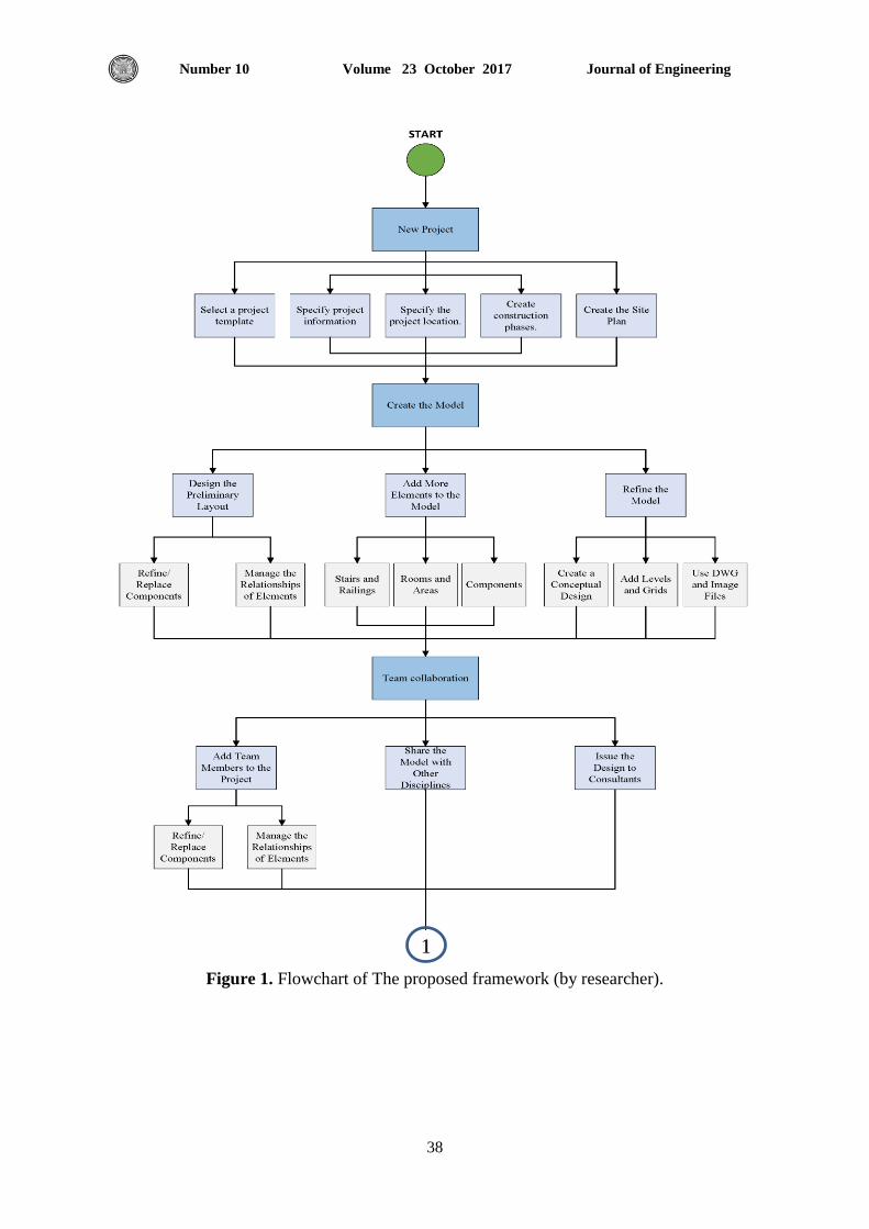
Journal of Engineering Volume 23 October 2017 Number 10
38
Figure 1. Flowchart of The proposed framework (by researcher).
1
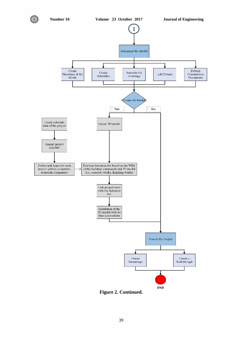
Journal of Engineering Volume 23 October 2017 Number 10
39
Figure 2. Continued.
1
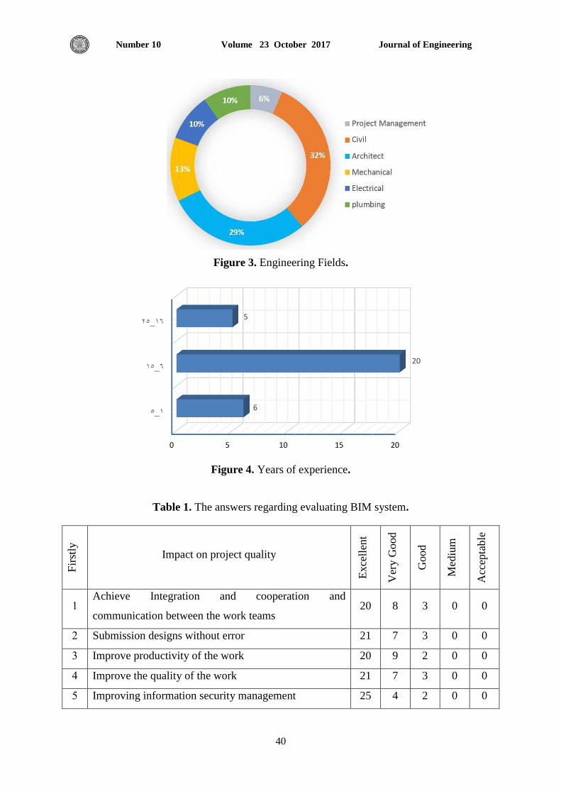
Journal of Engineering Volume 23 October 2017 Number 10
40
Figure 3. Engineering Fields.
Figure 4. Years of experience.
Table 1. The answers regarding evaluating BIM system.
Fir
stly
Impact on project quality
Exce
llen
t
Ver
y G
ood
Good
Med
ium
Acc
epta
ble
3 Achieve Integration and cooperation and
communication between the work teams 20 8 3 0 0
2 Submission designs without error 21 7 3 0 0
1 Improve productivity of the work 20 9 2 0 0
4 Improve the quality of the work 21 7 3 0 0
5 Improving information security management 25 4 2 0 0
0 5 10 15 20
1_5
6_15
16_25
6
20
5
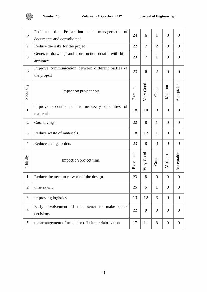
Journal of Engineering Volume 23 October 2017 Number 10
41
6 Facilitate the Preparation and management of
documents and consolidated 24 6 1 0 0
7 Reduce the risks for the project 22 7 2 0 0
8 Generate drawings and construction details with high
accuracy 23 7 1 0 0
9 Improve communication between different parties of
the project 23 6 2 0 0
Sec
ondly
Impact on project cost
Exce
llen
t
Ver
y G
ood
Good
Med
ium
Acc
epta
ble
3 Improve accounts of the necessary quantities of
materials 18 10 3 0 0
2 Cost savings 22 8 1 0 0
1 Reduce waste of materials 18 12 1 0 0
4 Reduce change orders 23 8 0 0 0
Thir
dly
Impact on project time
Exce
llen
t
Ver
y G
ood
Good
Med
ium
Acc
epta
ble
3 Reduce the need to re-work of the design 23 8 0 0 0
2 time saving 25 5 1 0 0
1 Improving logistics 13 12 6 0 0
4 Early involvement of the owner to make quick
decisions 22 9 0 0 0
5 the arrangement of needs for off-site prefabrication 17 11 3 0 0
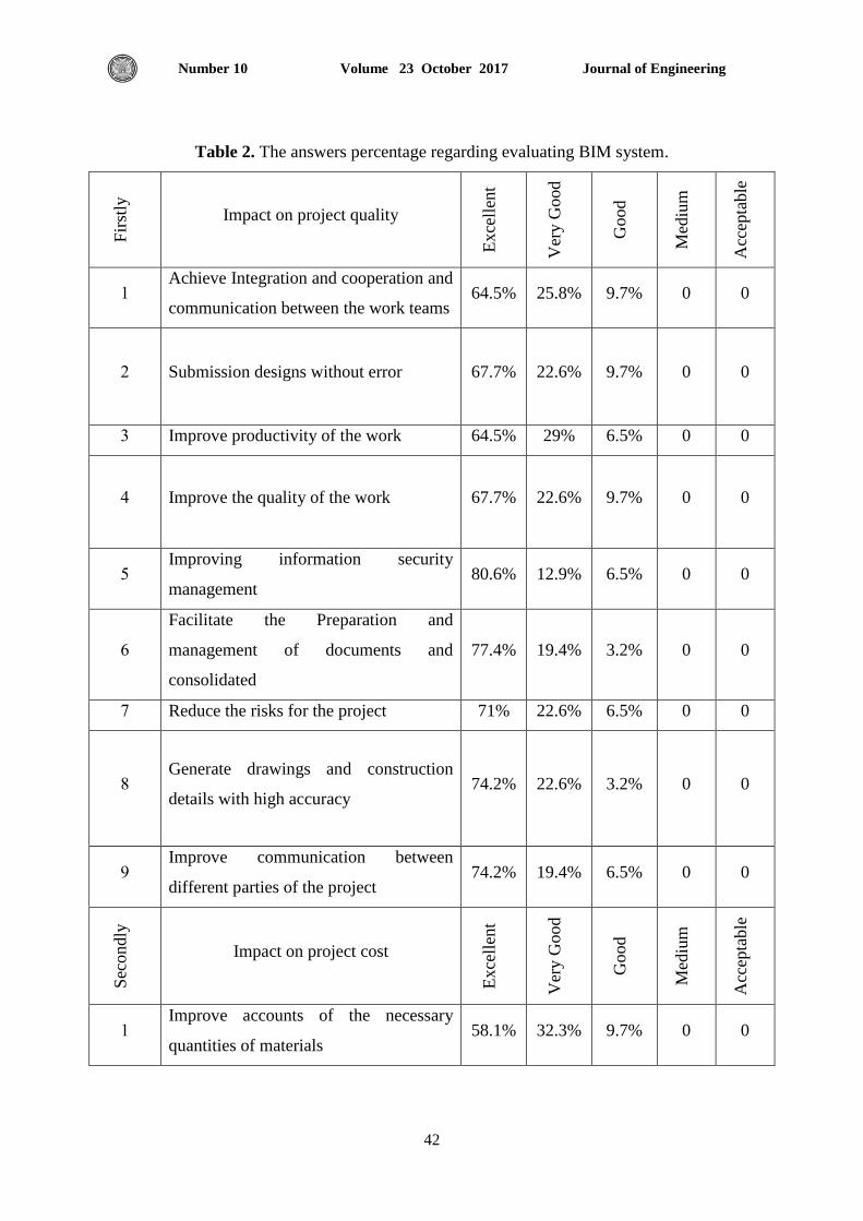
Journal of Engineering Volume 23 October 2017 Number 10
42
Table 2. The answers percentage regarding evaluating BIM system.
Fir
stly
Impact on project quality
Exce
llen
t
Ver
y G
ood
Good
Med
ium
Acc
epta
ble
3 Achieve Integration and cooperation and
communication between the work teams 64.5% 25.8% 9.7% 0 0
2 Submission designs without error 67.7% 22.6% 9.7% 0 0
1 Improve productivity of the work 64.5% 29% 6.5% 0 0
4 Improve the quality of the work 67.7% 22.6% 9.7% 0 0
5 Improving information security
management 80.6% 12.9% 6.5% 0 0
6
Facilitate the Preparation and
management of documents and
consolidated
77.4% 19.4% 3.2% 0 0
7 Reduce the risks for the project 71% 22.6% 6.5% 0 0
8 Generate drawings and construction
details with high accuracy 74.2% 22.6% 3.2% 0 0
9 Improve communication between
different parties of the project 74.2% 19.4% 6.5% 0 0
Sec
ondly
Impact on project cost
Exce
llen
t
Ver
y G
ood
Good
Med
ium
Acc
epta
ble
3 Improve accounts of the necessary
quantities of materials 58.1% 32.3% 9.7% 0 0
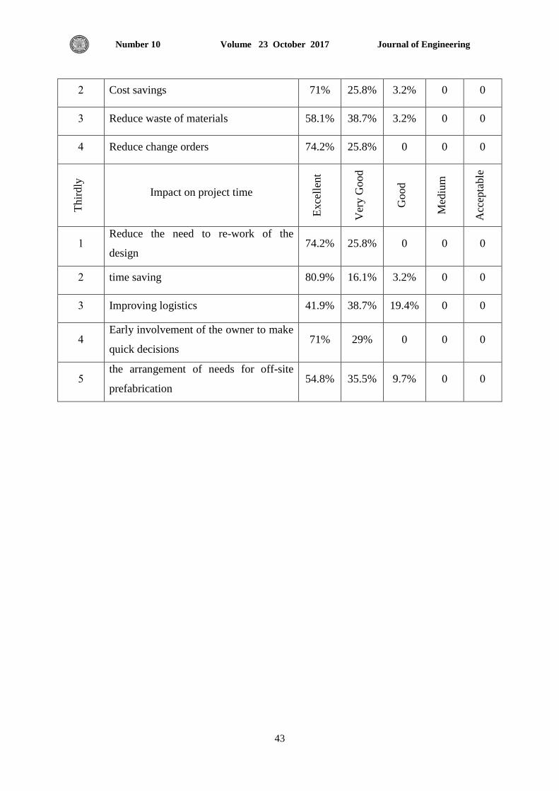
Journal of Engineering Volume 23 October 2017 Number 10
43
2 Cost savings 71% 25.8% 3.2% 0 0
1 Reduce waste of materials 58.1% 38.7% 3.2% 0 0
4 Reduce change orders 74.2% 25.8% 0 0 0
Thir
dly
Impact on project time
Exce
llen
t
Ver
y G
ood
Good
Med
ium
Acc
epta
ble
3 Reduce the need to re-work of the
design 74.2% 25.8% 0 0 0
2 time saving 80.9% 16.1% 3.2% 0 0
1 Improving logistics 41.9% 38.7% 19.4% 0 0
4 Early involvement of the owner to make
quick decisions 71% 29% 0 0 0
5 the arrangement of needs for off-site
prefabrication 54.8% 35.5% 9.7% 0 0
Journal of Engineering Volume 23 October 2017 Number 10
44
Improvement of Gypseous Soil Using Cutback Asphalt
Zainab Hassan Shakir Assistant Lecturer
Building and Construction Engineering Department, University of Technology/ Baghdad
ABSTRACT
Gypseous soils are widely distributed and especially in Iraq where arid area of hot climatic is
present. These soils are considered as problematic soils; therefore this work attends to improve
the geotechnical properties of such soil and reduce the dangers of collapse due to wetting
process. In this research, undisturbed soil sample of 30 % gypsum content from Karbala city is
used. The Single Oedometer collapse test is used in order to investigate the collapse
characteristics of natural soil and after treatment with 3%, 6%, 9%, 12% and 15% of Cutback
Asphalt. Moreover, two selected additive percentages (9% and 12%) are used to evaluate the
suitability of using the Cutback Asphalt for improvement of the bearing capacity of gypseous
soils. A steel model box is used for this purpose, the treatment depth is equal to one and twice
the footing width. The tests results showed that the total settlement of 25 mm of treated soil with
(MC-30) material can be achieved at vertical stress lower than that value required for natural
soil. Also, thickness of treated layer with (MC-30) material below the proposed foundation has a
significant effect on the value of bearing capacity of the soil. The rate of salt dissolved (C.V) is
extremely decreased especially at all percentages of Cutback Asphalt. The best bearing
improvement ratio is found at 9% asphalt and at a depth equal to foundation width. However, the
Cutback Asphalt can be successfully used by 12% for collapse potential treatment while it is not
suitable for improvement of the bearing capacity of gypseous soils.
Key words: gypsum soil, cutback asphalt, collapse potential.
السائلالسفلت ابأستخدام الجبسية التربةتثبيت
زينب حسن شاكر
يذسط يغاعذ
تغذاد /نركنخأندايع أالشاءاخ،أنثاء أ حذعلغى
لخالصهأ
راخ ححث ذراخذ اناؽك انماحه ي انعانى تشكم عاو تانعشاق عه خ انخظص جيحذدتاؽك حاندثغذرشش انرشب
انحاس. اناخ
حذحغ خظائض ز انرشت حن يحاننزنك ذف زا انثحث ا حاالاس حراخ انشاكم انذع ذعرثش ز انرشب ي انرشب
ذمهم خطش االاس عذ ذعشػا نهرشؽة .
حنهرشت حاالاس حانطال ع رحشانذى 30%كشتالء تغث خثظ حي يحافظ حزا انثحث ذى اعرخذاو رج انرشتف
تاعرخذاو فحض االديرش انفشد .
ح( تغثCutback Asphalt( )MC-30) جتاعرخذاو ياد حف ز انرشت االاس حيشكه حالرشحد يعاند حانذساع
تد ذظف انرشب حػعف عشع االعاط .رائح انعاند نعشع االعاط حتاعاق يغا %3,%6,%9,%12,%15
ػحد انرائح ا ك أ. %01االاس ان حؽال حي انع انخطش تغثة اسذفاع ل حذع حيشكهراخ حتاا ذشت حاندثغ
ايثم نالعفهد ف يحر حنغا حئض االاس نهرشب اندثغتداذ ف ذحغ خظا (MC-30ع ) اعرخذاو ياد االعفهد
. حذذسد جغث االعفهد انؼاف تظس جتضاد حاندثغ حهرشتانرحم ن ح. تاء عه رنك فا ذخفغ لاته% 01 حتغث حانرشت
ذحد اخاد mm 25( ذظم ان انثؽ انكه انثانغMC-30االعفهد ) جتاد حانعاند حنمذ اظشخ رائح انفحض ا انرشت
حا عك انطثم . كا حانطثع حفظ يمذاس انثؽ نهرشتاالخاد انعد انطهب نهحظل عه حعد الم ي ل
ا يعذل رتا . حانرحم نهرشب اندثغ حنا ذاثش كثش عه يمذاس لاته ( ذحد االعاطMC-30تاد االعفهد ) حانعاند
Journal of Engineering Volume 23 October 2017 Number 10
45
نرحغ حخذ ا احغ غثانرائح حي خالل دساع االعفهد انؼاف. حغث جعذ صاد حخاط جتظس كثشا االيالذ خفغ
تد رائح انفحص اؼا تأ يادج االعفهد .االعفهد عم عك يغا ان عشع االعاط جي ياد9%انرحم حف لاته
.حتهح انرحم نهرشب اندثغدحد تشكم كثش ف ذحغ خظائض االاس نكا غش يالئح نرحغ لا
1. INTRODUCTION
Gypseous soils are of the most complex materials that challenge the geotechnical engineers. It is
a well-known fact that gypseous soils demonstrate high bearing capacity and very low
compressibility when they are in the dry state. Conversely sudden collapsible disposal was
reported when the gypseous soils are exposed to water. The collapsibility of gypseous soils
scores from the direct contact of water. The rate of dissolution of gypsum depends primarily on
environmental changes in moisture content generating from fluctuation of ground water table
and/or surface water, permeability and state of flow conditions in addition to the type and
content of gypsum, Al-Saoudi et.al, 2013. The dissolution of gypsum particles within the soil
mass due to wetting can cause many problems to the engineering structures and road network the
structure of gypseous soil can be transformed from stable condition to unstable when undergo to
increase in moisture content. The gypseous soil is defined as soil that contains sufficient
quantities of gypsum (calcium sulphate), FAO, 1990. This soil is commonly formed at dry state
particularly due to the cementation of the soil particles by gypsum, but the issue turnoff intricate
when the water flow through the gypseous soils causing nominate and reasonable collapse
behavior in the soil structure. Many studies have been conducted on gypseous soils in Iraq
because they are covering a wide area of nearly 31.7% of the surface sediments of Iraq with
gypsum content ranging between 10-70%, Ismail, 1994, and are 0.6% of the world, Alphen and
Romero, 1971. Gypsiferous soils have been studied in the past within the classical framework of
soil mechanics that is related to saturated condition. As such, they are characterized as
collapsible, problematic soils that suffer large settlement and have significant loss of strength
under long term of flooding, Khalid, 2013. When salt firmness soils are undergoing softening
due to raising in moisture content can cause degeneration of same gypsum. Practically softening
can occur in various ways like local shallow wetting, deep local wetting. Many problems have
been notified on damages happened to structures supported on gypseous soils like cracks,
overturning of structures. These problems are very dangerous, thus improvement of gypseous
soils are urgently necessary. On the other hand, asphalt material can be used as improvement
material for the problematic soils where the main function of asphalt is to reduce the effect of
water on gypsum particles and to increase the strength parameters of the soil, Al-Obaydi et.al,
2007. In Iraq, asphalt is a cheap and available material; it can be easily used to improve the
properties of gypseous soil. Many forms of asphalt are available such as asphaltic bitumen, tars,
Cutback Asphalt and emulsion asphalt or bitumen can be added to the base soil of roads,
Kadhim, 2014.
The Cutback Asphalt is most common and economical type of asphaltic materials used for soil
stabilization especially medium-curing types where it’s produced from the refineries, Transport
and Road Research Laboratory, 1987. Moreover, Jasim, 2015 assessed the durability of
asphalt stabilized gypseous soil by using emulsion asphalt. It was stated that after exposing the
specimens to cycles of (heating – cooling), the undrained shear strength increased up to 10
cycles then decreased with further increased number of cycles. The dissolution of gypsum due to
Journal of Engineering Volume 23 October 2017 Number 10
46
distillation, irrigation and hail water or from other provenance is a risky case in gypseous soil
age. This process will command to on undue and sometimes tragic settlement. Shear strength of
soil will minimize as a result of this process. The safety and good execution of the foundation of
structures particularly in hydraulic structures and earth structure like embankments and dams
will be administered by the changes in the properties of these soils.
2. PREVIOUS EXPERIENCES
The behavior of gypseous soils and its improvements attempts were carried out by many
research works which can be outlined as follows:
Al-Rawi, 1971 suggested that both cutback and emulsion asphalt could be used to stabilize Iraqi
soils.
Epps et.al, 1971 studied the mixture of sandy soil with asphalt and found that 4-5% is the
optimum cutback percent for maximum stability.
Al-Kawaaz, 1990 studied the behavior of sandy gypesous soil asphalt mix in Oedometer test; the
main conclusion is the increase in binder content.
Al-Shakayree, 2003 showed that, in sandy soil the maximum dry unit weight decreases, and the
optimum water content increases with the increase in gypsum content result in increase in
rebound strain.
Al-Obaidi, 2003 used two materials in order to improve the collapsibility characteristics of
sandy gypseous soil with gypsum content of 70% from Al-Ramady city west of Iraq. The first
material was Glass sand as a natural residual material, and the second was powder of destroyed
ceramic as a residual of industrial material. Both materials succeeded to improve the collapse
deformation of gypseous soil with more than 50%, where the collapse potential reduced from
about 10% to 4.5%.
Al-Harbawy and Al-Khashab, 2004 reported the effect of stabilizing gypseous soil using liquid
asphalt types such as cutback and emulsion on its behavior of shear strength is considerably
observed. Addition of liquid asphalt provides cohesion strength to the soil mass and also acts as a
waterproofing agent. Cutback Asphalt increases the resistance of gypseous soil to permeability,
such resistance increases as void ratio increases.
Al-Saidi et.al, 2011 demonstrated that the stabilizing of gypseous soil using the optimum fluid
content of 16% (5%Cutback Asphalt+11% water) led to improve the unconfined compressive
strength, compressibility, and rebound consolidation. The additive acts as waterproofing of
gypseous soil. While under absorbed condition, lime-cutback mixture was used in order to
satisfy the base course construction requirements.
Aziz, 2011 showed that fuel oil is a good material to modify the basic properties of the gypseous
soil such as collapsibility and permeability, which are the main problems of this soil. The fuel oil
Journal of Engineering Volume 23 October 2017 Number 10
47
provides an appropriate amount of the cohesion in the soil which is suitable for carrying the
loads from the structure.
3. MATERIALS
3.1 Gypseous Soil
The soil samples were taken from Eaan Tamur city, Karbala governorate, south west of Iraq.
From a depth of 3m up to 6m below the natural ground level. The samples are packed in a
double nylon bags and transported to the soil mechanics laboratory at University of Technology
in Baghdad for testing.
3.2 Asphalt
The type of asphalt used in this research is medium curing cutback (MC-30) liquid asphalt which
is used in maintenance of surface layers of asphalt produced by Al- Dora Refinery in Baghdad
Governorate. This type is fabricated by one step:
91.2 % [(40-50) asphalt cement] + 8.8% [kerosene] → (MC-30) (1)
Properties of Cutback Asphalt (MC-30) used are given in Table 1.
4. PROPERTIES OF GYPSEOUS SOILS
4.1 Physical Properties
The summary of the physical tests results are shown in Table 2.
4.1.1 Grain size distribution
The grain size distribution was determined according to (ASTM D422- 63, (2007)) using dry
sieving. The grain size distribution curve of the soil is clarified in Fig.1.
4.1.2 Specific gravity
The specific gravity was determined according to BS 1377: 1975, Test No.6 (B). Kerosene was
used instead of distilled water because of the dissolving action of gypsum by water, Head, 1980.
4.1.3 Water content
This was determined in accordance to BS 1377:1975, Test (A).The oven dry temperature was
kept at 45◦C due to dehydration of gypsum.
4.1.4 Compaction test
Standard compaction tests are carried out on soil sample to determine the water content –unit
weight relationship according to, ASTM D698, 2000.
4.2 Chemical Properties
The gypsum content is determined according to the method presented by, Al-Mufty and Nashat,
2000. This method consists of oven drying the soil at C until the weight of the sample
becomes constant. The weight of the sample at C is recorded, then the same sample is dried
at C for 24 hrs and the weight is recorded again. The gypsum content is then calculated
according to the following equation:
Journal of Engineering Volume 23 October 2017 Number 10
48
X (%) =⟦
⟧
x4.778x100 (2)
Where:
x= gypsum content (%).
C.
.
4.3 Geotechnical Properties
4.3.1 Collapsibility
Gypseous soils exhibits collapse behavior as results of volume change upon wetting. The term of
"collapse"commonly refers to the deformation of the soil mass due to reduction in its volume
when exposed to water. Jennings and Knight, 1957 proposed a single Oedometer collapse test
to predict the collapsibility of the soil under the foundation. The collapse potential C.P is defined
as:
C.P =
(3)
Where:
∆e = the difference in void ratio of the sample at a specific stress.
= the natural void ratio.
The severity of collapse according to the collapse potential is shown in Table 3.
It was found that, the value of collapse potential for the natural soil is (10%), and according to
the specification listed in Table.3 the case of severity is classified as trouble to severe, and hence
the soil needs to be treated.
5. EXPERIMENTAL PROGRAM
The experimental program in this study can be categorized into the following groups:
Group (A): Consisting of five mixtures which were prepared from various percentages of
Cutback Asphalt and added to the natural gypseous soil samples in order to perform the testing
program. The percentages of Cutback Asphalt are 3%, 6%, 9%, 12%, and 15% and expressed as
binder content (%) these values were chosen depending on numerous references that stated and
specified. The range of the binder content used by, Kadhim, 2014 who employed percentages of
binder was equal 2%, 4%, 6%, 8%, 10%. The mixed samples were tested by single Oedometer
collapse test, the sample was prepared in Oedometer ring with initial condition unit weight equal
12.5
.The loading sequence of single Oedometer collapse test is 25, 50, 100, 200 and 400 kPa,
and the loading interval is 1 hour for each vertical stress. However, the loading duration for the
collapse stress of 200 kPa is 24 hours for both unsaturated (drying) and saturated (soaking)
Journal of Engineering Volume 23 October 2017 Number 10
49
conditions. The loading sequence of single Oedometer test is according to Jennings and Knight,
1957 and ASTM D5333, 2003.
Group (B): The geotechnical model tests of this group were conducted in proposed steel model
box with dimensions of 30 cm in length, 30 cm in width and 35 cm in depth. The filter layer of
fine gravel material was placed to a depth of 5cm from the bottom of steel box. The soil was
prepared at the same properties used in group A. The soil strata extend to the depth of 2B from
the surface filter where B is the footing width. The model is soaked with water by means of
flexible pipe connected at the container bottom. Two values of collapse potential (6.2% and
2.6%) were chosen to be treated, which are corresponding to asphalt contents of (9% and 12%)
respectively. These values of asphalt contents represented the best treatment percentages, which
succeeded to obtain significant reduction in collapse potential from single Oedometer collapse
test. This treatment can be induced to a depth of 6 cm and 12 cm under model foundation. A
square footing of dimension 6 × 6 cm was placed on the surface of the treated soil layer and
subjected to vertical static loading where the loads are applied at regular time intervals of (4-15)
min according to ASTM D1194, 1994 for each load increments. One dial gauge was used and
the vertical settlement of the footing for each increment of load was recorded.
6. DISCUSSION OF TEST RESULTS
6.1 Collapse Test
The results of single Oedometer collapse test can be shown in Table 4. and Fig.2 The reduction
in collapse potential of gypsum soil is clearly observed as a result of adding the Cutback Asphalt
material (MC-30) as shown in Fig.2. The collapse potential (C.P) is considerably decreased from
10% to 2.6% with the increase in the percentage of (MC-30) to 12%. This behavior is attributed
to the action of asphalt material as water proofing for gypsum particles, in other words the (MC-
30) film fill the air voids in soil mass as well as covering the gypsum grain and reduce its ability
to dissolve by water. The improvement results showed that 12% of Cutback Asphalt additive is
the optimum value for collapse reduction. Adding (MC-30) material such as 15% leads to a
reverse behavior where the deformation of the soil mass increased dramatically as shown in
Fig.2 The increasing of soil deformation with high percentage of (MC-30) asphalt can be related
to two reasons, the first reason is the lubricant action of (MC-30) layer which causes sliding of
soil particles each one on other during loading. The second one can be related to the increase of
the total volume and liquidity of the soil mass with the increase of (MC-30) content which may
cause direct decrease in the value of dry density and increases the collapse potential.
6.2 Effect of Cutback Additive on the Coefficient of Salt Dissolved
Firstly, the material of Cutback Asphalt additive tries to reduce the water accessibility to the
gypsum particles. Then, the presence of Cutback Asphalt as a thin layer surrounded the soil
particle also leads to decreasing the interaction between the water and gypsum subsequently, the
reaction between them would be slow. Thus, the salts dissolution need more time to be
significantly settled. It is worthy mentioned, that (C.V) is expressed as the rate of settlement of
soil or by other words represents the coefficient of salt dissolved during soaking.
Journal of Engineering Volume 23 October 2017 Number 10
50
The addition of Cutback Asphalt to the gypseous soil shows a good reduction in settlement value
so that the asphalt percentage has a proportional relation with the time required for collapse to
occur. Table 5 presents the variation the coefficient of salt dissolved with different amounts of
asphalt ranging from 0 to 15%. It is noticed that, adding (0%, 3%, 6%, 9%, 12%, and 15%)
asphalt require to (8, 11, 13, 15, 31, and 33) minutes to achieve 90% of total dissolve of salts.
However, the test results indicated the high suitability of Cutback Asphalt to be used as
improvement material for collapsibility of gypseous soils. The results also demonstrate an
excellent indication on the asphalt efficiency to be used in reducing the gypsum soil collapse.
The effect of asphalt content on the coefficient of salt dissolved can be displayed in Fig.3 to 8.
From the Fig.3 to 8 it was observed that, the irregular shapes of curves upon loading are
attributed to the addition of asphalt to the gypseous soil reduce the amount of dissolved gypseous
and coefficient of salt dissolved (C.V).
6.3 Bearing Capacity Test
The bearing capacity of gypseous soil after treatment with 9% and 12% of (MC-30) asphalt was
investigated using proposed foundation model with treatment depth of 6 cm and 12 cm. The
results of load-settlement relationship shown in Fig.11 indicate that, the bearing capacity
decreases after treatment with (MC-30) material. The total settlement of 25 mm of treated soil
can be achieved at vertical stress lower than those value required for natural soil. Moreover,
treatment of gypseous soil to a depth deeper than 1B (i.e. 6 cm) causes more reduction in the
value of bearing capacity of the soil. This behavior can be attributed to decreasing of the shear
strength of the soil with adding of (MC-30) material as a result of decrease in angle of internal
friction. Moreover, the load distribution under proposed foundation extends normally to a depth
of 2B, therefore in this case study it can be observed that the bearing capacity in the first case of
treatment (i.e. to a depth 2B of 12 cm) is lower than the first case of treatment (i.e. to a depth 1B
of 6 cm). That is clearly shown in Fig.13.
On the other hand at a depth equivalent to foundation width, it was noted that the bearing
improvement ratio (B.I.R) increased from 136% to 192% when the asphalt amount in soil
decreased from 12% to 9% respectively. This could be explained that the best percent of
improvement was gained when the amount of asphalt is 9%. In other words, any increase in
asphalt percent could lead to a negative effect on the bearing capacity. This could be attributed to
the amount of asphalt existed in the soil at 12% which causes increasing the soil compressibility
and reducing the shear strength at this percent more than its effect on soil collapse; hence,
reducing the bearing capacity and increasing the settlement value. This is clear in Fig.11. When
the depth of soil-asphalt mixture equals to double foundation width, the asphalt presence at any
percent at this depth reduces significantly the bearing capacity because: a large area of influence
zone beneath the foundation would be increased in terms of compressibility and decreased in
terms of modulus of elasticity. Thus, the shear properties (C and φ) would considerably reduce
and this explains the reduction in (B.I.R) value with respect to asphalt percent. Fig.13 clarifies
the result.
Journal of Engineering Volume 23 October 2017 Number 10
51
In sequence the settlement values after using the admixture was less than their corresponding
values without admixture. The value of settlement reduction ratio (S.R.R) decreased to 0.52 and
0.68 at an admixture ratio of 12% and 9% respectively. Therefore, the best percent in reducing
the settlement at depth (asphalt + soil) equal to foundation width was 9%, as clearly is shown in
Fig. 11.
Regarding the stabilized soil with asphalt at a depth of double value of foundation width, it was
found that, the settlement in both cases of asphalt 9% and 12% increases the settlement with
respect to that calculated from the untreated soils. Thus, stabilizing at a depth of 2B at any
admixture percent would has a negative effect on the settlement values. This is clearly shown in
Fig.13.
7. CONCLUSIONS
1. The Cutback Asphalt (MC-30) material can be used successfully to improve the collapsibility
characteristics of gypseous soil and the optimum (MC-30) asphalt recommended is 12 %.
2. The bearing capacity of the soil decreases after treatment with (MC-30) asphalt. Thus this
additive is not suitable for improvement of the bearing capacity of gypseous soils.
3. The total settlement of 25 mm of treated soil with (MC-30) material can be achieved at
vertical stress lower than that value required for natural soil.
4. The thickness of treated layer with Cutback Asphalt material below the proposed foundation
has a significant effect on the value of bearing capacity of the footing.
5. The rate of collapse (C.V) extremely decreases using all the percentages of Cutback Asphalt.
6. The best percent of bearing improvement ratio (B.I.R) and settlement reduction ratio (S.R.R)
are acquired at a depth equal to foundation width, and when the asphalt content is 9%.
REFERENCES
Al-Harbawy, A.F.Q., Al-Khashab, M.N., 2004, The Effect of Emulsified Asphalt Addition
on Some of the Engineering Properties of Expansive Clayey Soils, Eng. And Technology,
Vol.2, No. 23, PP.51-71.
Al-Kawaaz, N., 1990, Characteristics of Soil Asphalt Mixture, M.Sc. Thesis, College of
Engineering, University of Baghdad.
Al-Mufty, A. A, and Nashat, E. H., 2000, Gypsum Content Determination in Gypseous
Soil and Rock, Proceedings of the Jordanian International Mining Conference
Amman, Vol.2, PP.485-492.
Al-Obaydi, A. A. H., Mohmmed, Y. T., and Omar, M. E. T., 2007, The Use of Liquid
Asphalt to Improve Gypseous Soils, internet reference www.iasj.net/iasj.
Al-Obaidi, Q.A.J., 2003, Studies in Geotechnical and Collapsible Characteristics of
Gypseous soil, M.Sc. Thesis, Civil Engineering Department, College of Engineering, Al-
Mustansiriyah University, Baghdad, Iraq.
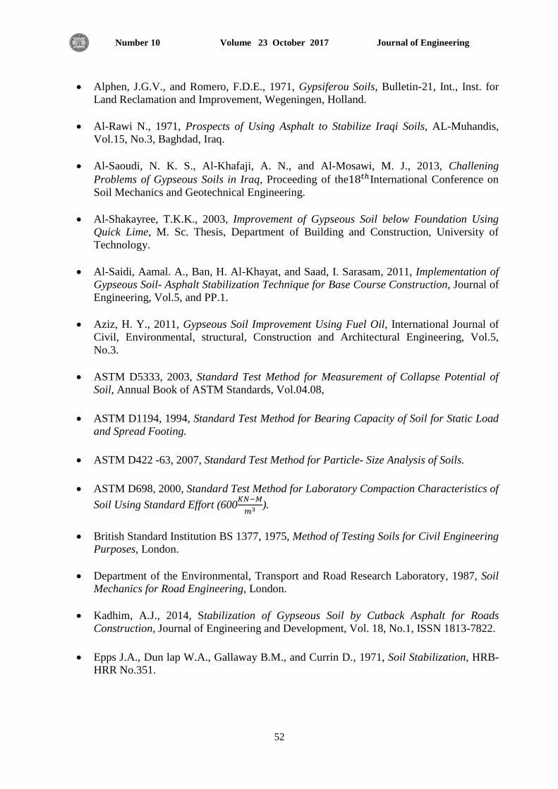
Journal of Engineering Volume 23 October 2017 Number 10
52
Alphen, J.G.V., and Romero, F.D.E., 1971, Gypsiferou Soils, Bulletin-21, Int., Inst. for
Land Reclamation and Improvement, Wegeningen, Holland.
Al-Rawi N., 1971, Prospects of Using Asphalt to Stabilize Iraqi Soils, AL-Muhandis,
Vol.15, No.3, Baghdad, Iraq.
Al-Saoudi, N. K. S., Al-Khafaji, A. N., and Al-Mosawi, M. J., 2013, Challening
Problems of Gypseous Soils in Iraq, Proceeding of the International Conference on
Soil Mechanics and Geotechnical Engineering.
Al-Shakayree, T.K.K., 2003, Improvement of Gypseous Soil below Foundation Using
Quick Lime, M. Sc. Thesis, Department of Building and Construction, University of
Technology.
Al-Saidi, Aamal. A., Ban, H. Al-Khayat, and Saad, I. Sarasam, 2011, Implementation of
Gypseous Soil- Asphalt Stabilization Technique for Base Course Construction, Journal of
Engineering, Vol.5, and PP.1.
Aziz, H. Y., 2011, Gypseous Soil Improvement Using Fuel Oil, International Journal of
Civil, Environmental, structural, Construction and Architectural Engineering, Vol.5,
No.3.
ASTM D5333, 2003, Standard Test Method for Measurement of Collapse Potential of
Soil, Annual Book of ASTM Standards, Vol.04.08,
ASTM D1194, 1994, Standard Test Method for Bearing Capacity of Soil for Static Load
and Spread Footing.
ASTM D422 -63, 2007, Standard Test Method for Particle- Size Analysis of Soils.
ASTM D698, 2000, Standard Test Method for Laboratory Compaction Characteristics of
Soil Using Standard Effort (600
).
British Standard Institution BS 1377, 1975, Method of Testing Soils for Civil Engineering
Purposes, London.
Department of the Environmental, Transport and Road Research Laboratory, 1987, Soil
Mechanics for Road Engineering, London.
Kadhim, A.J., 2014, Stabilization of Gypseous Soil by Cutback Asphalt for Roads
Construction, Journal of Engineering and Development, Vol. 18, No.1, ISSN 1813-7822.
Epps J.A., Dun lap W.A., Gallaway B.M., and Currin D., 1971, Soil Stabilization, HRB-
HRR No.351.
Journal of Engineering Volume 23 October 2017 Number 10
53
FAO, 1990, Management of Gypseous Soils, Soil Resources, Management and
Conservation Service, FAO Land and Water Development Division.
Head, K.H., 1980, Manual of Soil Laboratory Testing, Vol. 1, Prentch Press, London.
Ismail, H.N., 1994, The Use of Gypseous Soils, Symposium on the Gypseous Soils and
Their Effect on Strength, NCCL, Baghdad.
Jasim .A. L., 2015, Assessing the Durability of Asphalt Stabilized Gypseous Soil
Embankment, M. Sc. Thesis, Department of Civil Engineering, University of Baghdad.
Jennings J.E., and Knight K., 1957, The Additional Settlement of Foundation Sandy
Subsoil on Wetting, Proceeding 4th Int. Conf. Soil mechanics and foundation
engineering, Vol.1, PP.316-319.
Khalid, I. A., 2013, Effect of Gypsum on The Hydro Mechanical Characteristics of
Partially Saturated Sandy Soil, Ph.D Thesis, College of Cardiff School of Engineering,
Cardiff University, British.
NOMENCLATURE
Cc = coefficient of curvature.
Cu = coefficient of uniformly.
C.P = collapse potential (%).
C.V = coefficient of salt dissolve.
= is the natural void ratio.
Gs = specific gravity.
X = gypsum content (%).
C.
.
angle of internal friction.
∆e = is the difference in void ratio of the sample at a specific stress.
Figure 1. Grain size distribution of soil.
0
20
40
60
80
100
0.010.1110
(%)
fin
er p
erce
nt
grain size (mm)
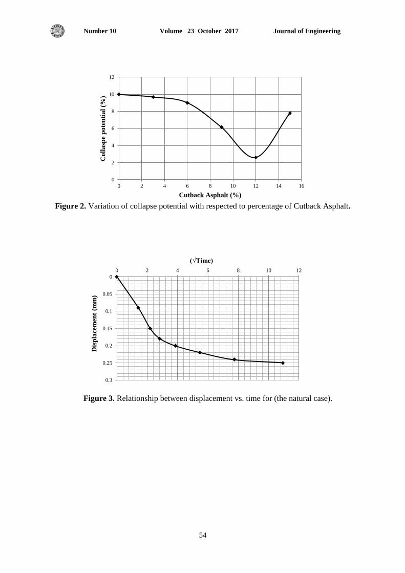
Journal of Engineering Volume 23 October 2017 Number 10
54
Figure 2. Variation of collapse potential with respected to percentage of Cutback Asphalt.
Figure 3. Relationship between displacement vs. time for (the natural case).
0
2
4
6
8
10
12
0 2 4 6 8 10 12 14 16
Co
lla
spe
po
ten
tia
l (%
)
Cutback Asphalt (%)
0
0.05
0.1
0.15
0.2
0.25
0.3
0 2 4 6 8 10 12
Dis
pla
cem
ent
(mm
)
(√Time)
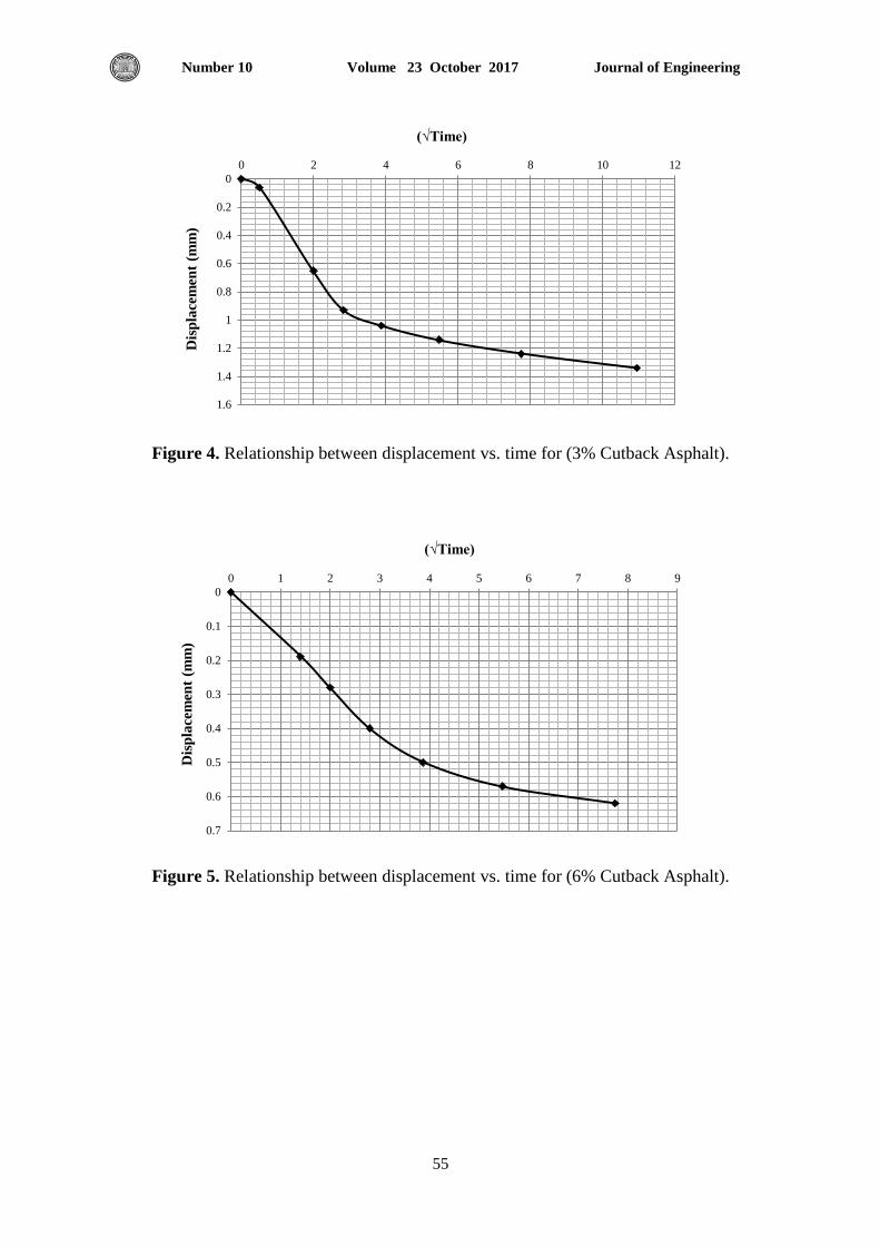
Journal of Engineering Volume 23 October 2017 Number 10
55
Figure 4. Relationship between displacement vs. time for (3% Cutback Asphalt).
Figure 5. Relationship between displacement vs. time for (6% Cutback Asphalt).
0
0.2
0.4
0.6
0.8
1
1.2
1.4
1.6
0 2 4 6 8 10 12
Dis
pla
cem
ent
(mm
)
(√Time)
0
0.1
0.2
0.3
0.4
0.5
0.6
0.7
0 1 2 3 4 5 6 7 8 9
Dis
pla
cem
ent
(mm
)
(√Time)
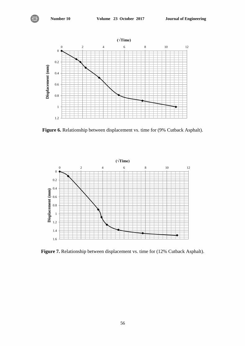
Journal of Engineering Volume 23 October 2017 Number 10
56
Figure 6. Relationship between displacement vs. time for (9% Cutback Asphalt).
Figure 7. Relationship between displacement vs. time for (12% Cutback Asphalt).
0
0.2
0.4
0.6
0.8
1
1.2
0 2 4 6 8 10 12D
isp
lace
men
t (m
m)
(√Time)
0
0.2
0.4
0.6
0.8
1
1.2
1.4
1.6
0 2 4 6 8 10 12
Dis
pla
cem
ent
(mm
)
(√Time)
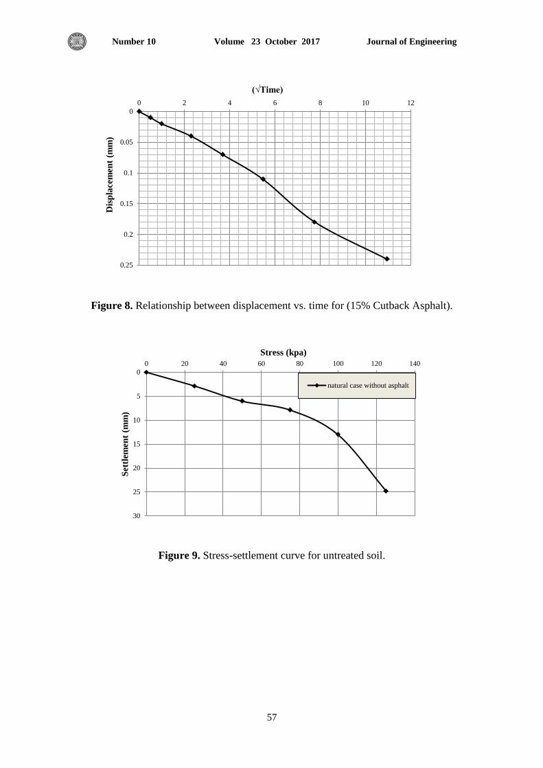
Journal of Engineering Volume 23 October 2017 Number 10
57
Figure 8. Relationship between displacement vs. time for (15% Cutback Asphalt).
Figure 9. Stress-settlement curve for untreated soil.
0
0.05
0.1
0.15
0.2
0.25
0 2 4 6 8 10 12D
isp
lace
men
t (m
m)
(√Time)
0
5
10
15
20
25
30
0 20 40 60 80 100 120 140
Set
tlem
ent
(mm
)
Stress (kpa)
natural case without asphalt
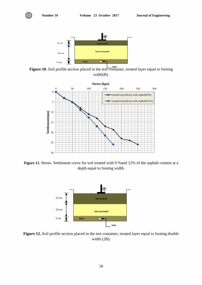
Journal of Engineering Volume 23 October 2017 Number 10
58
Figure 10. Soil profile section placed in the test container, treated layer equal to footing
width(B).
Figure 11. Stress- Settlement curve for soil treated with 9 %and 12% of the asphalt content at a
depth equal to footing width.
Figure 12. Soil profile section placed in the test container, treated layer equal to footing double
width (2B).
0
5
10
15
20
25
30
0 50 100 150 200 250 300
Set
tlem
ent(
mm
)
Stress (kpa)
treated layer(6cm) with asphalt(9%)
treated layer(6cm) with asphalt(12%)
Filter
Inlet
Soil treated
Soil untreated 19 cm
5 cm
6 cm
Soil treated
Soil untreated
Inlet
Filter
12 cm
13 cm
5 cm
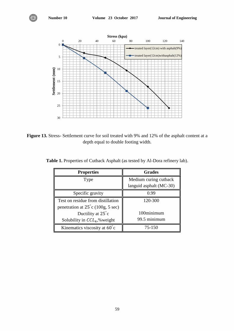
Journal of Engineering Volume 23 October 2017 Number 10
59
Figure 13. Stress- Settlement curve for soil treated with 9% and 12% of the asphalt content at a
depth equal to double footing width.
Table 1. Properties of Cutback Asphalt (as tested by Al-Dora refinery lab).
Properties Grades
Type Medium curing cutback
languid asphalt (MC-30)
Specific gravity 0.99
Test on residue from distillation
penetration at c (100g, 5 sec)
Ductility at c
Solubility in ,%weight
120-300
100minimum
99.5 minimum
Kinematics viscosity at c 75-150
0
5
10
15
20
25
30
0 20 40 60 80 100 120 140
Set
tlem
ent
(mm
)
Stress (kpa)
treated layer(12cm) with asphalt(9%)
treated layer(12cm)withasphalt(12%)
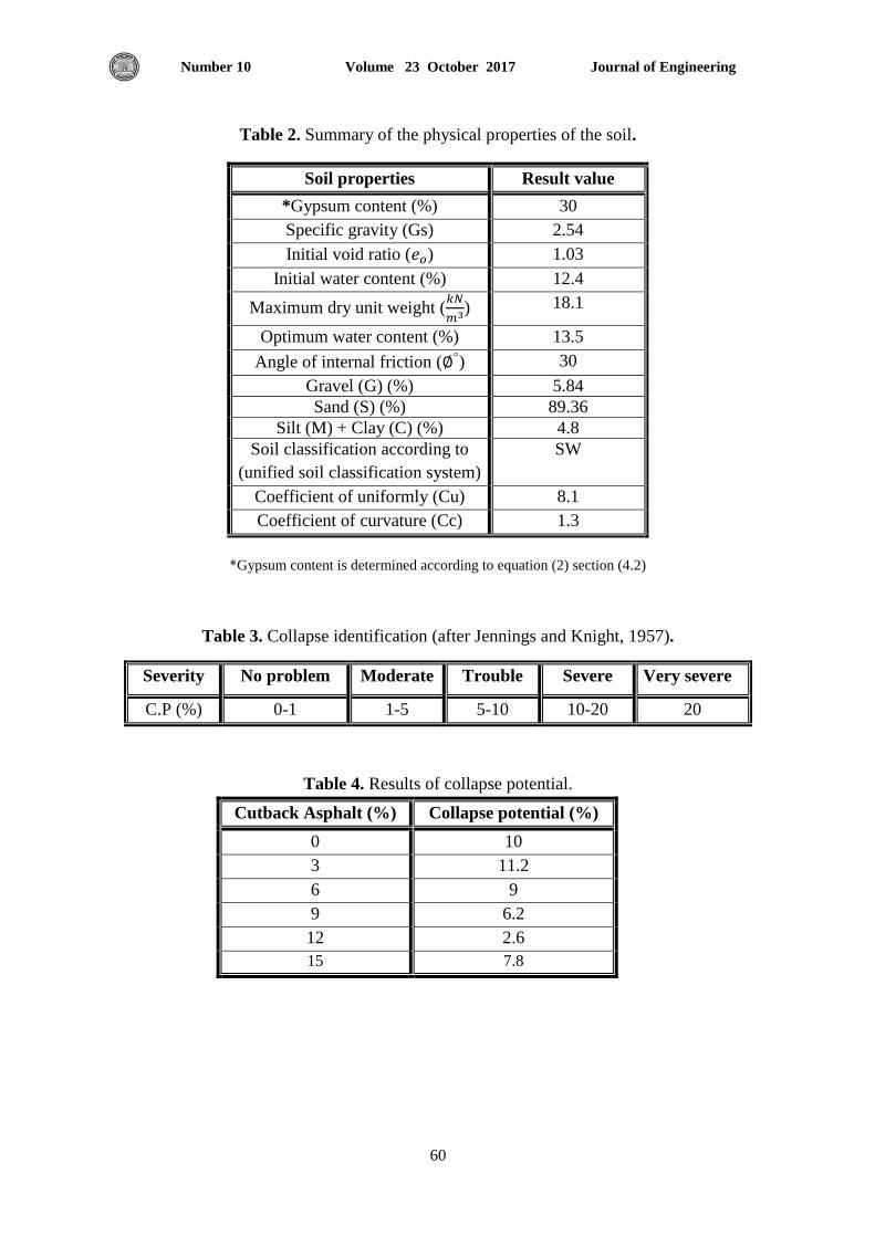
Journal of Engineering Volume 23 October 2017 Number 10
60
Table 2. Summary of the physical properties of the soil.
Soil properties Result value
*Gypsum content (%) 30
Specific gravity (Gs) 2.54
Initial void ratio ( ) 1.03
Initial water content (%) 12.4
Maximum dry unit weight (
) 18.1
Optimum water content (%) 13.5
Angle of internal friction ( ) 30
Gravel (G) (%) 5.84
Sand (S) (%) 89.36
Silt (M) + Clay (C) (%) 4.8
Soil classification according to
(unified soil classification system)
SW
Coefficient of uniformly (Cu) 8.1
Coefficient of curvature (Cc) 1.3
*Gypsum content is determined according to equation (2) section (4.2)
Table 3. Collapse identification (after Jennings and Knight, 1957).
Severity No problem Moderate Trouble Severe Very severe
C.P (%) 0-1 1-5 5-10 10-20 20
Table 4. Results of collapse potential.
Cutback Asphalt (%) Collapse potential (%)
0 10
3 11.2
6 9
9 6.2
12 2.6
15 7.8

Journal of Engineering Volume 23 October 2017 Number 10
61
Table 5. The coefficient of salt dissolve results with respect to asphalt percentages.
Asphalt content (%) C.V
0 8 0.432
3 11 0.3
6 13 0.26
9 15 0.2301
12 31 0.108
15 33 0.102
Journal of Engineering Volume 23 October 2017 Number 10
62
Optimization of Surface Roughness For Al-alloy in Electro-chemical
Machining (ECM) Using Taguchi Method
Mostafa Adel Abdullah
Dept. of Production Engineering and Metallurgy
University of Technology/Baghdad. Iraq
Email [email protected]
Dr. Shukry Hammed Aghdeab Safaa Kadhim Ghazi
Assistant Prof Assistant Lecturer
Dept. of Production Engineering and Metallurgy Dept. of Production Engineering and Metallurgy
University of Technology/Baghdad. Iraq University of Technology/Baghdad. Iraq
Email [email protected] Email [email protected]
ABSTRACT
Electro-chemical Machining is significant process to remove metal with using anodic
dissolution. Electro-chemical machining use to removed metal workpiece from (7025)
aluminum alloy using Potassium chloride (KCl) solution .The tool used was made from copper.
In this present the optimize processes input parameter use are ( current, gap and electrolyte
concentration) and surface roughness (Ra) as output. The experiments on electro-chemical
machining with use current (30, 50, 70)A, gap (1.00, 1.25, 1.50) mm and electrolyte
concentration (100, 200, 300) (g/L). The method (ANOVA) was used to limited the large
influence factors affected on surface roughness and found the current was the large influence
factors with (72.17%) . The results of the optimization of comparison of experimental and
prediction conditions current at level-1(30 A), gap at level-1 (1.00mm ) and electrolyte
concentration at level-1(100(g/L)) shown the average experiments and prediction surface
roughness (1.352 μm) and (1.399 μm) respectively..
Keywords: Electro-chemical machining, surface roughness, optimization, taguchi, ANOVA.
تاكىش طرقة باستخذاو انكهروكاوي انتشغم ف نسبكة االننىو انسطحة انخشىنة ايثهة
هللا عبذ عادل يصطفى
ساعذ ذسط
بغذاد اىعشاق/ اىخنىخت اىداعت/ اىعاد االخاج ذست
غازي كاظى صفاء غضب حذ شكري. د
ساعذ ذسط ساعذ اسخار
بغذاد اىعشاق/ اىخنىخت اىداعت/ اىعاد االخاج ذست بغذاد اىعشاق/ اىخنىخت اىداعت/ اىعاد االخاج ذست
انخالصة
اىخشغو اىبحث زا ف. حيه احاله باسخخذا اىعاد إلصاىت ةؤثش طشقت اىخشغو اىنشما
ميسذحيه يح ) باسخخذا( 5025) األى سبائل اىن اىشغىتت عذ صاىسخعو إل اىنشما
اىفدة ،اىخاس يت باسخعاهذخاى ف ز اىعيت ححذذاىخغشاث ح . اىحاط صع سخخذتاى داةاأل (اىبحاس
مخشج اىسطح خشت حن.األثو ىيحصه عي اىخداسب ححيو ىخص حامش أسيب اسخخذبا. اىحيه حشمض
اك ابش(50 ،50 ،30) باسخعاه ق حاس اخشج اىخشغو اىنشما اىخداسب(. 5024) ع األى ىسبنت
ىخحذذ ا ( أفا) أسيب اسخخذا ح(. ىخش/ غشا( )300 ،200 ،100) هحياى حشمض ي( 1.50 ،1.25 ،1.00) فدة
Journal of Engineering Volume 23 October 2017 Number 10
63
خائح٪(. 52.15) بسبت احأثش اىعاو امبش ما اىخاس أ خذ . اىسطح خشت عي خأثشاىمبش ن اىعاو
اىسخ ف اىفدة ،ابش(30) االه اىسخ اىخاس باسخعاه اىخدشبت اىظشف سخاث ب ىقاستا األثو االسخغاله
اىسطح خشتىي اىخبؤ اىخداسب خسط أظش()غشا/ىخش( 100) االه اىسخ ف هحياى حشمض ي ) 1.00) االه
.اىخاى عي انش (1.311) انش (1.352 )
.اىخشت اىسطحت ،االثيت ،حامش،افا,اىنشما اىخشغو انكهات انرئسة :
1. INTRODUCTION
Electro-chemical machining (ECM) is a non-conventional process that depends on the
removal of workpiece atoms by electro-chemical dissolution process, Al-Hofy, 2005.The
removal process of use anodic dissolution, where anode is workpiece and tool is cathode. To
dissolve metal from the work piece, electrolyte is push on the gap between metal and electrode,
while the current is passed on the cell ,Hiba, 2011, focused on the effect of the change in
current , gap on surface roughness of . The results obtained show that, increasing of the gap
size between the tool and the workpiece from (1mm) to (3mm) leads to increase of (46%) in
the surface roughness of the workpiece, increasing of the current density from (2.4485
Amp/cm2) to (3.6728 Amp/cm
2) leads the to decrease in surface roughness of the workpiece by
approximately (31%). Used the Statistical Package for the Social Sciences (SPSS) software to
prediction the results. Babar, et al, 2013, discuss the effect and condition optimization of ECM
process used titanium based alloy. The condition of process that use are applied voltage,
electrolyte concentration sodium chloride (NaCl) and feed ,which optimization according to
material removal rate (MRR) as output. Analysis of variation contribution to performance
characteristics. The results shown that the large influnance condition is voltage and then the
electrolyte concentration and feed. The raise material removal rate (MRR) lead to raise in
electrolyte concentration and voltage. The optimum values of process parameters are
(electrolyte concentration (15 wt%), applied voltage (20 V)), tool feed rate (0.32mm/min).
Mohanty, et al., 2014, studied the effect of process parameter (voltage, electrolytic
concentration and feed rate) on performance characteristics such as roughness average (Ra)
affecting the surface roughness. The surface roughness initially increases with concentration,
but it decreases at maximum concentration. The optimal condition for SR was found to be at (30
g/l) concentration of when electro-chemical machining used a tool of copper in an aqueous
sodium chloride (NaCl). ANOVA were used to study the effect of parameters on cutting
machining. It was observed that an increase in voltage where is roughness average (Ra)
decreased. Voltage was found to be significantly electrolyte, (15V) voltage and ( 0.2 mm/min)
feed rate. Habib, 2014, studied the effect of (ECM) cutting condition (voltage, electrode feed,
and current) on the surface roughness. Taguchi method and analysis of variance (ANOVA) are
used to optimization the electro-chemical machining process. The results show that maximum
factor effect on surface roughness are current with (53%)then feed with (21%), voltage
(11.5%). The optimum parameter(30V) voltage, (1 mm/min) feed rate used to get better
roughness average (Ra=3.218 μm).
2. THEORY OF TAGUCHI
Taguchi discovers a novel conception for the quality control method named as (Taguchi
parameter design). The method stated that the quality of manufactured part must be computed
by the deviation amount from the required value. He takes into consideration not only the
Journal of Engineering Volume 23 October 2017 Number 10
64
operation mean, but also the variation magnitude or (noise) created with manipulating the inputs
parameters or operation variables. The technique is focus on two major groups; a unique matrix
type called orthogonal array (OA), all the columns include number of experiment depending on
the level number for the control factor, in addition to (signal to noise ratio) S/N Abbas,2009 .
n
i
iyn
NS1
2)(
1log10/ ; i=1, 2,……… ……………(1)
The formula is utilized to calculating signal to noise ratio are given Eq(2):
n
i iynNS
1
2 )1(1
log10/ ; i=1,2,………. ……………(2)
Where, yi the measurements of output , and n is the measurements of input.
The final design of input parameter for work done according to MINITAB16 software as follow:
STAT DOE Taguchi Create Taguchi Design
3. ANALYSIS OF VARIANCE
The results using (ANOVA) to explain the effect of machining condition on the
roughness average (Ra) depend on machining condition current, gap and electrolyte construct
while others are independent variables., F- ratio refer to mean square error and (%) percent is
refer to influence rate of operation variables to (Ra), Mohammed,2016.
4. EXPERIMENTAL WORK
In electro-chemical machining design using drilling machine and other parts accessories
with workpiece (7024)Aluminum alloy .The percentages of chemical composition is given in
Table 1. with anode workpiece dimension (40x 30) mm and thickness (20) mm as shown in
Fig 1,with using nine simple with change in machining parameter and constant machining
time(5)min and different depth of hole.
4.1 The ECM machine
The ECM cell used in these experiments is shown in Fig 2. It consists of :
The drilling machine, workpiece fixture, electrolyte pump and power supply.
The drilling machine Provides a rigid base and good control of the tool feeding with
manual controlling to maintain the gap size between tool and workpiece. workpiece fixture is
made from cast iron. Pumps the electrolyte in the reaction chamber to gap between tool and
workpiece. The used power supply in the experiment is a (D.C) welding machine with current
(5 A/10 V-400 A/36V) type CEBORA .
Journal of Engineering Volume 23 October 2017 Number 10
65
4.2 Cathode Tool
In this paper, copper tool used with purity is (99.9%). The reason for using copper metals
is because they are (easy to machine, have high electric conductivity and high corrosion
resistance). with diameter (10 mm) , length (5 cm) and roughness average (Ra) (0.475 μm) as
shown in Fig 3.
4.3 Electrolyte
The electrolyte use to creates appropriate conditions for anodic dissolution ( workpiece),
conducts the current and removes the waste from the gap. In this work as KCl as electrolyte
with compost, listed in Table 2.
4.4 Design of Experiments
The total of experiments machining is (nine experiments) with (3) levels (3) parameters
as (33). A partial factorial design was done use (9)to study the effect of parameter on surface
roughness (Ra). The cutting parameters used ( current, gap and electrolyte construct). The levels
of cutting parameters are listed in Table 3.
4.5 Surface Roughness measurements
The Pocket Surf gauge is portable surface measurements use ,with selectable traverse
length (1, 3 or 5)mm as shown in Fig 4 .
5. RESULTS AND DISCUSSION
The experiments work using the design parameter array Table 4. as shown in Fig 5. The
complete response data to get minimize surface roughness. The Signal-to-Noise ratio (S/N)
should be as small as possible, because the quality characteristic “smaller is better” was used.
S/N values were calculated from Eq.(1), and the results have been arranged in the last column
of array in Table 4. The results were analyzed by using main effects for both surface roughness
values and signal-to-noise ratio, and ANOVA analyses. Then the estimate results which
obtained checked experimentally to insure the estimate value. In terms of the average effects,
the average value of surface roughness for each parameter (A, B and C) listed in Table 4.
5.1 Analysis of Variance
The results are analyzed by using (ANOVA) method to find the effect of machining
condition on the surface roughness, surface roughness as the output, current, gap and electrolyte
concentration as input. Therefore, the most influential parameter is the current (72.17%), gap
(17.81%) and minimize effect electrolyte concentration (5.63%) as shown in Table 5.
"
Journal of Engineering Volume 23 October 2017 Number 10
66
5.2 Optimal Design Conditions For Surface Roughness
The main effects figure used to find the better design parameter to get the better surface
roughness and to select the better machining parameters using Fig 6. which shows the main
effect figure conditions for minimum surface roughness were: current at level-1 (30 A), gap at
level-1 (1.00 mm and electrolyte concentration at level-1(100(g/L)).
The Fig 6.and Fig 7. depending on data in Table 4. Because of using “smaller is better”
quality characteristic in this study, The difference (max-min) parameter of three levels for each
parameter indicates that the current has the highest effect on the surface roughness followed by
a gap and electrolyte concentration.
6. CONCLUSION
This research used Taguchi’s design (minimum number of experiments can use this
method )for get optimum parameter with lowest surface roughness,.
The Maximum surface roughness when current (70 A) , gap (1.50 mm) and electrolyte
concentration (300(g/L)).
Through ANOVA method , found current is very important factor influnes (72.17%) on
surface roughness.
The compare of experimental and prediction conditions levels ( A1B1C1 ) (current at level-
1(30 A), gap at level-1 (1.00 mm ) and electrolyte concentration at level-1(100(g/L)). shown
the average experiments measure and prediction surface roughness from Taguchi (1.352 μm)
and (1.399 μm) respectively .
REFERENCES
Al-Hofy. H,2005, Advanced Machining Process, Nontraditional and Hybrid Machining
Process, Mcgraw-Hill Company, Egypt.
Hiba. H. Alwan , 2011,Study of Some Electrochemical Machining Characteristics Of Steel
Ck35, M.Sc Thesis University Of Technology, Iraq.
- Babar.P. D, B. R. Jadhav ,2013,Experimental Study On Parametric Optimization Of
Titanium Based Alloys (Ti-6al-4v) In Electrochemical Machining Process, International
Journal Of Innovations In Engineering And Technology , Vol. 2, pp.171-175,India.
Mohanty. A, Gangadharudu Talla, S. Dewangan, S.Gangopadhyay,2014 ,Experimental Study
of Material Removal Rate, Surface Roughness & Microstructure In Electrochemical
Machining Of Inconel 825, International & All India Manufacturing Technology, India.
Habib. S. S,2014 , Experimental Investigation of Electrochemical Machining Process Using
Taguchi Approach, International Journal of Scientific Research In Chemical Engineering
,Vol.1,No. 6, Pp. 93-105, Egypt, .
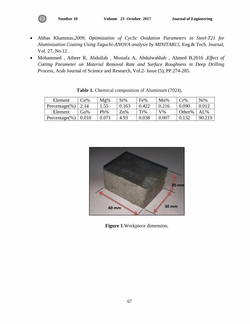
Journal of Engineering Volume 23 October 2017 Number 10
67
Abbas Khammas,2009, Optimization of Cyclic Oxidation Parameters in Steel-T21 for
Aluminization Coating Using Taguchi-ANOVA analysis by MINITAB13, Eng.& Tech. Journal,
Vol. 27, No.12 .
Mohammed , Atheer R, Abdullah , Mostafa A, Abdulwahhab , Ahmed B,2016 ,Effect of
Cutting Parameter on Material Removal Rate and Surface Roughness in Deep Drilling
Process, Arab Journal of Science and Research, Vol.2- Issue (5), PP.274-285.
Table 1. Chemical composition of Aluminum (7024).
Element Cu% Mg% Si% Fe% Mn% Cr% Ni%
Percentage(%) 2.14 1.55 0.163 0.422 0.216 0.090 0.012
Element Ga% Pb% Zn% Ti% V% Other% AL%
Percentage(%) 0.010 0.071 4.93 0.038 0.007 0.132 90.219
Figure 1.Workpiece dimension.
40 mm 30 mm
20 mm
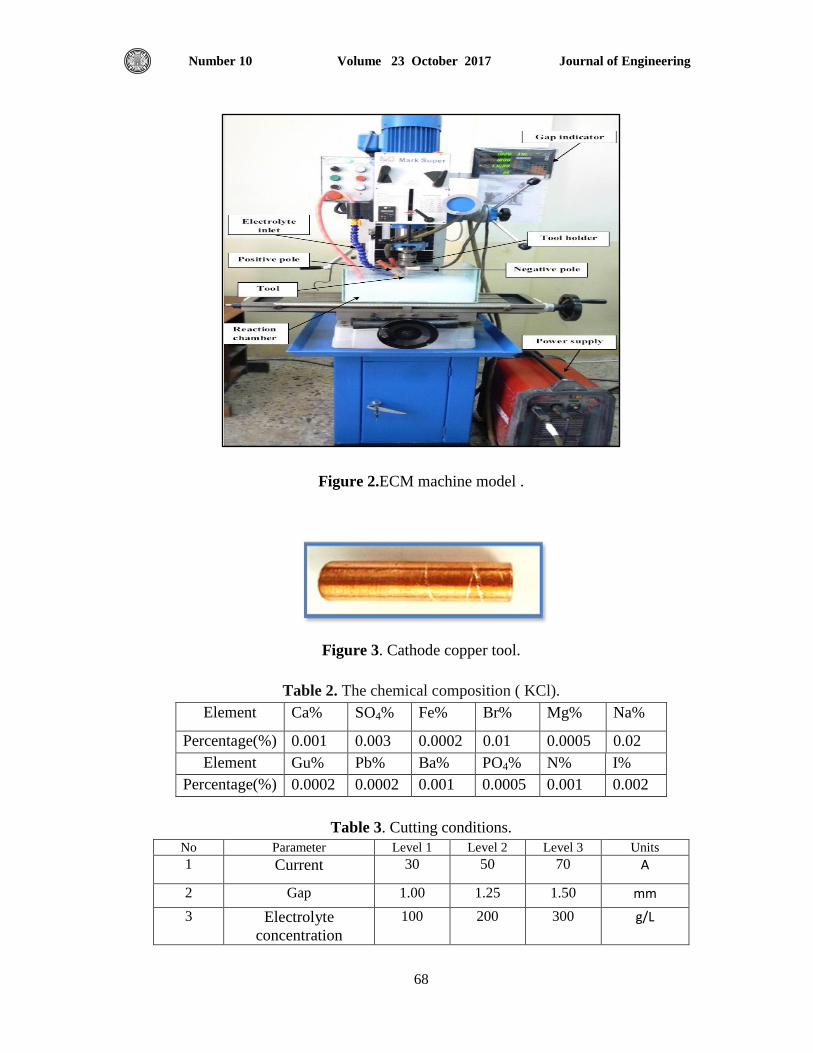
Journal of Engineering Volume 23 October 2017 Number 10
68
Figure 2.ECM machine model .
Figure 3. Cathode copper tool.
Table 2. The chemical composition ( KCl).
Element Ca% SO4% Fe% Br% Mg% Na%
Percentage(%) 0.001 0.003 0.0002 0.01 0.0005 0.02
Element Gu% Pb% Ba% PO4% N% I%
Percentage(%) 0.0002 0.0002 0.001 0.0005 0.001 0.002
Table 3. Cutting conditions.
Units Level 3 Level 2 Level 1 Parameter No
A 70 50 30 Current 1
mm 1.50 1.25 1.00 Gap 2
g/L 300 200 100 Electrolyte
concentration
3
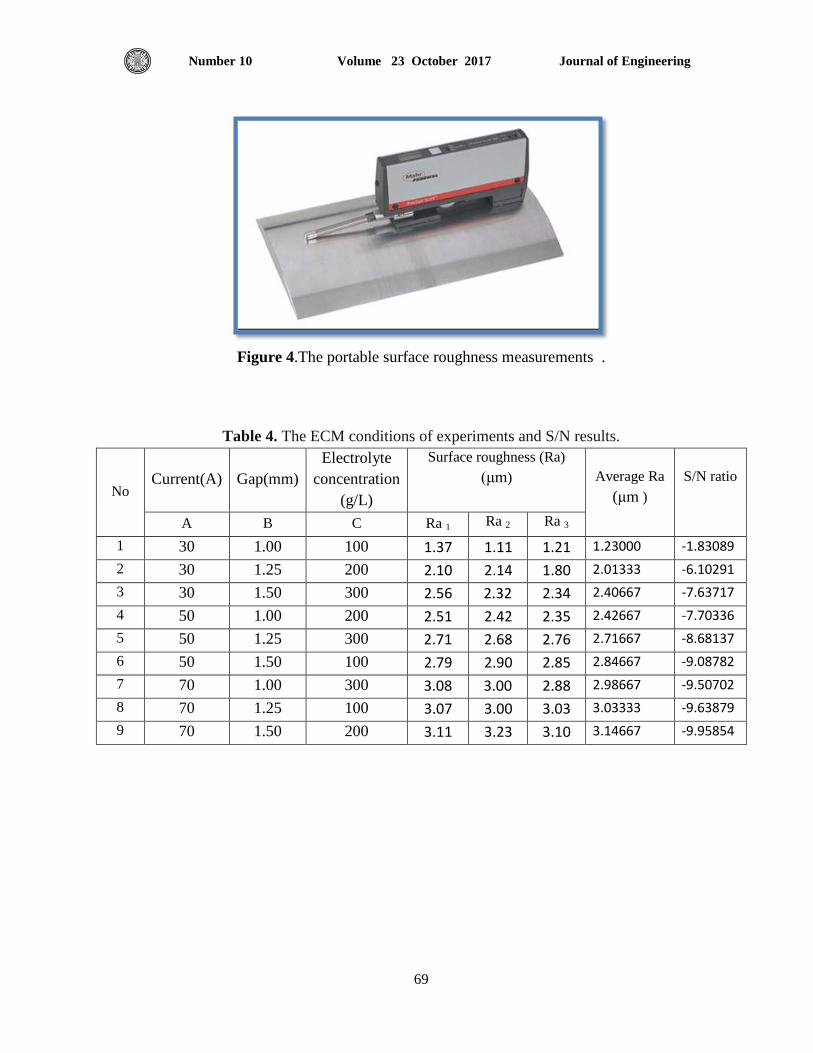
Journal of Engineering Volume 23 October 2017 Number 10
69
Figure 4.The portable surface roughness measurements .
Table 4. The ECM conditions of experiments and S/N results.
S/N ratio
Average Ra
(μm )
Surface roughness (Ra)
(μm)
Electrolyte
concentration
(g/L)
Gap(mm) Current(A) No
Ra 3 Ra 2 Ra 1 C B A
-1.83089 1.23000 1.21 1.11 1.37 100 1.00 30 1
-6.10291 2.01333 1.80 2.14 2.10 200 1.25 30 2
-7.63717 2.40667 2.34 2.32 2.56 300 1.50 30 3
-7.70336 2.42667 2.35 2.42 2.51 200 1.00 50 4
-8.68137 2.71667 2.76 2.68 2.71 300 1.25 50 5
-9.08782 2.84667 2.85 2.90 2.79 100 1.50 50 6
-9.50702 2.98667 2.88 3.00 3.08 300 1.00 70 7
-9.63879 3.03333 3.03 3.00 3.07 100 1.25 70 8
-9.95854 3.14667 3.10 3.23 3.11 200 1.50 70 9
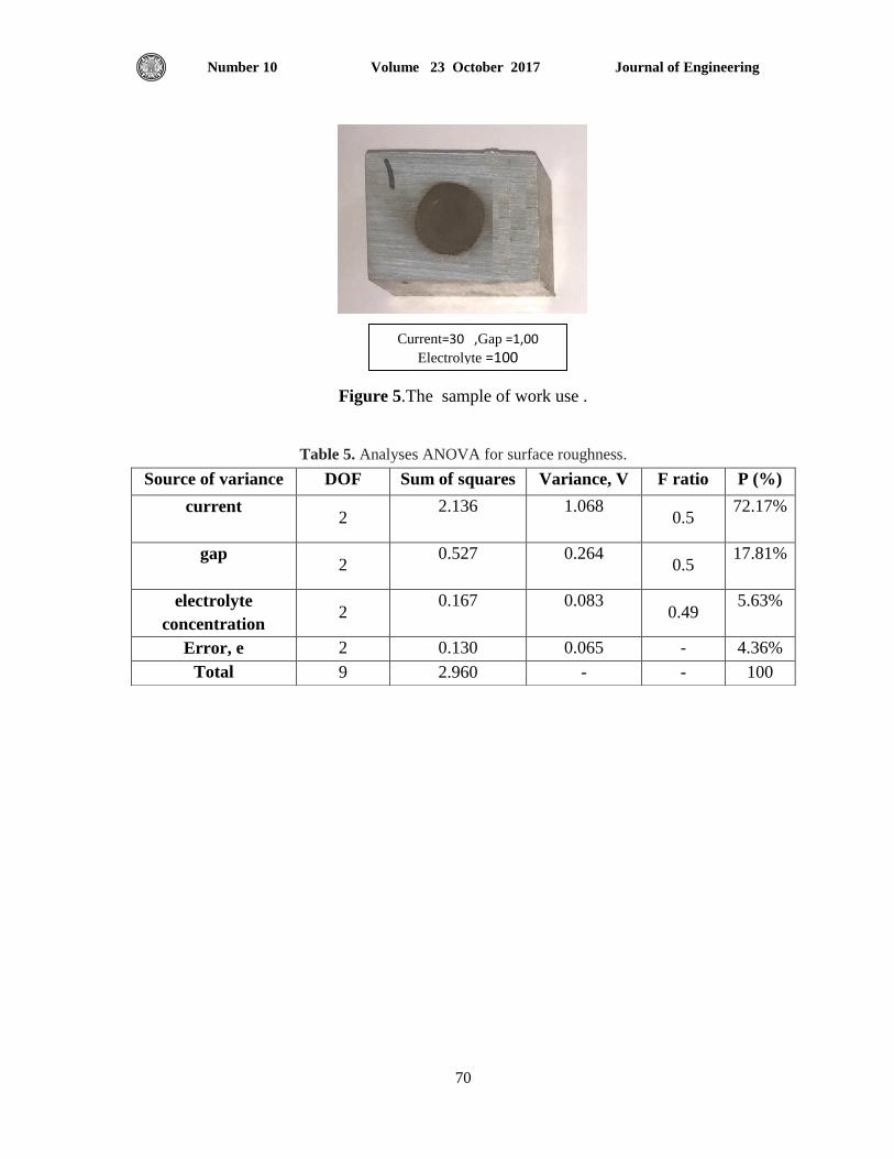
Journal of Engineering Volume 23 October 2017 Number 10
70
Figure 5.The sample of work use .
Table 5. Analyses ANOVA for surface roughness.
Source of variance DOF Sum of squares Variance, V F ratio P (%)
current 2
2.136 1.068 0.5
72.17%
gap 2
0.527
0.264
0.5
17.81%
electrolyte
concentration 2
0.167
0.083
0.49
5.63%
Error, e 2 0.130 0.065 - 4.36%
Total 9 2.960 - - 100
Current=30 ,Gap =1,00
Electrolyte =100
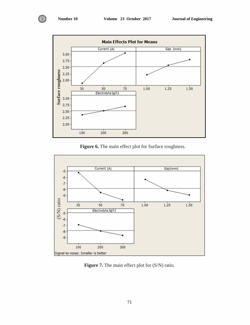
Journal of Engineering Volume 23 October 2017 Number 10
71
Figure 7. The main effect plot for (S/N) ratio.
Figure 6. The main effect plot for Surface roughness.
(A) (mm)
(g/L)
(A) (mm)
(g/L)
Su
rfa
ce r
ou
gh
nes
s (S
/N)
rati
o
Journal of Engineering Volume 23 October 2017 Number 10
72
Dry Sliding Wear Behavior of EN25 Steel Treated by Different Quenching
Media
Bassam Ali Ahmed
Assistant Lecturer
Department of Electromechanical Engineering
University of Technology
Email: [email protected]
ABSTRACT
The present investigation aims to study the effect of heat treatment by quenching in different
quenching media (salt water, water and oil) following by tempering on wear resistance of EN25
steel. EN25 steel is an alloy of medium carbon low alloy steel which is used for many applications
requiring high tensile strength and wear resistance such as connecting rods, adapters and in power
sectors extensively. The specimens are machined to 20 mm in length and 10 mm in diameter. This
study is done by two stages: The first stage is done by austenitizing EN25 steel to 850 for 1 hr
by quenching the specimens in three different quenching media and then tempered at 300 in air.
While the second stage is performed by wear test. Dry sliding wear test is done by using pin –on-
disc technique by varying the loads as 5, 10, 15, 20 and 25 N, also varying the time as 5, 10, 15,
20, 25 and 30 min respectively. The microstructure examination, hardness and followed roughness
tests are also done for the specimens before and after wear test. The results of this work showed
that an improving in wear resistance and hardness for the specimen quenched by salt water more
than for water and oil. At the same time the roughness decreasing for the specimen quenched by
salt water more than for water and oil.
Key Word: EN25 steel, quenching heat treatment, quenching media, wear.
المعالج بأوساط تقسية مختلفة En 25 لى االنزالقي الجاف للفوالذسلوك الب
بسام علي أحمد
يذسط يغاعذ
قغى انذعت انكشيكاكت
انجايعت انخكنجت
الخالصة
انعايهت انحشاست بانخقغت ف اعاط يخخهفت )ياء يانح، ياء، صج( عهى يقايت انبهى ذف انبحذ انحان نذساعت حأرش
عبكت ي فالر يخعط انكاسب يخفض انغبائكت غخخذو ف عذة حطبقاث انخ En 25. انفالر En 25نهفالر
يهى 02 بطلحخطهب يقايت شذ يقايت بهى عانخ يزم ارسع انخطم ،انحالث قاطعاث انقذسة. حى حشغم انعاث
زالد اعاط حقغت يخخهفت عذ دسجت يهى . اجشج ز انذساعت بشحهخ: االنى حى فا حقغت انعاث ب 02قطش
و 052حشاست o
و 022بعذ رنك حخى عهت انشاجعت عذ عاعت، 0نذة o
اناء. ف فعاعت ي رى انخبشذ 0نذة
انقشص -عهى -باعخخذاو حقت انغاسانشحهت انزات اجشي اخخباس انبهى. حى اخخباس انبهى االضالق انجاف با ف
Journal of Engineering Volume 23 October 2017 Number 10
73
دققت عهى انخان. 02،05،02،05،02،5حى حغش انضي بقذاس كزنك ، ح 05،02،05،02،5 رنك بخغش االحال
كزنك حى فحض انبت انجشت اجشج اخخباساث انظالدة انخشت قبم بعذ اخخباس انبهى.
باناء انانح اكزش يا عه نهعاث انقغاة اظشث خائج انبحذ ححغ ف يقايت انبهى انظالدة نهعت انقغاة
باناء انضج. بفظ انقج قظا انخشت نهعت انقغاة باناء انانح اكزش يا عه نهعاث انقغاة باناء
.انضج .، يعايهت حشاست بانخقغت ، أعاط انخقغت ، انبهى EN25فالر الكلمات الرئيسية:
1. INTRODUCTION
Today steel is an important alloy for the rapid development of technologies to obtain the
best performance of service; this can be achieved by different heat treatments processes,
Murugan, and Mathews, 2013. Heat treatment is defined as the heating of such carbon or
alloying steel depending on the percentage of carbon and then cooling to change particulate
characteristics of an alloy to achieve a suitable for a certain kind of application, Fadara, et al.,
2011. Heat treatment affected on mechanical properties such as strength, hardness and ductility
and also improving wear resistance. The purpose of heat treatment for the carbon steel is to
alter the microstructure by using a certain heating and then cooling in a suitable quenching
media to obtain the preferred characteristics, Ismail, et al., 2016. Wear is defined as surface
phenomena including an important three mechanisms acting simultaneously, such as adhesive
wear, abrasive wear, and erosive wear. Thus the heat treatment is important to reduce the wear
of machinery components at minimum level, Naveena, et al., 2015. Many researchers were
worked about heat treatment of steel such as Jasiwal, et al. 2015, they studied the effect of
different quenching media such as cold water, hot water and vegetable oil on the microstructure
and hardness of AISI 1050 carbon steel. While Motagi, and Bhosle, 2012, studied the effect of
heat treatment by quenching and tempering on mechanical properties and microstructure of two
different steel alloys with and without copper. Whilst Alabi, et al., 2012, studied the effect of
the temperature of the water as a quenchant on mechanical properties of two different medium
carbon steel containing 0.33 wt.%C and 0.4 wt. %C. Whilst Tukur, et al., 2014, were studied
the effect of quenching heat treatment at 900Cofor 45min and then tempering at aurous
tempering temperature 250Co, 350C
o, 450C
o and 550C
o on mechanical properties (tensile
strength, hardness) of medium carbon steel. The results of this work showed that increasing the
hardness, yield strength, ductility and the optimum values of the mechanical properties attained
at temperature of 250Co, while Karthikeyan, et al., 2014, studied the effect of subzero
treatment on hardness, toughness and the amount of retained austenite present in the structure
of EN24 steel alloy. They are using two different heat treatments in this work, the conventional
heat treatment (CHT) and shallow cryogenic treatment (SCT). The results of this investigation
reveals that the amount of the retained austenite for heat treatment (SCT) less than 2%, but for
heat treatment (CHT) about 15%, at the sometime increasing in toughness and ductility.
Journal of Engineering Volume 23 October 2017 Number 10
74
2. EXPERIMENTAL PROCEDURE
2.1. Material Used
The selected material for this work is EN25. Table 1 and Table 2 show the chemical
composition and mechanical properties of EN25 steel respectively, Funda, 2012.
2.2. Preparation of The Specimens
The EN25 steel specimens have been prepared by machining them to suitable dimensions,
20 mm in length and 10 mm in diameter. Then all the specimens are grinded with emery paper
(320, 500 and 1000 m) by using Al2O3 with 1 m in size and polished with suitable polishing
cloth by using diamond paste.
2.3. Heat Treatment
The prepared test specimens were adapted to treat by quenching. The specimens were
heated at 850co for 1hr. in an electrical furnace. After heating, the specimens were cooled
rapidly in three different quenching media (salt water, water and oil). After quenching, the
specimens were tempered at 300 for 1 hr. and then cooling in air Senthilkumar, and
Ajiboye, 2012. The electrical furnace used in this work as shown in Fig.1.
2.4. Hardness Test
The hardness values of all the specimens before and after hardening by quenching were
measured by Vickers method using 20 Kg for 15 Sec. Vickers hardness number can be
calculated by using the following formula, Bolton, 1988. For each specimen three readings
were taken to define the average value of the hardness.
V.H.N (1)
3. WEAR TEST
Wear test is carried out by using pin-on-disc technique to define the wear rate for all the
specimens before and after heat treatment by quenching in the different quenchants (salt water,
water and oil). Fig.2 shows the setup of wear test.
The specimens of this project are machined to suitable dimensions 20mm in height and 10mm
in diameter. Specimens for wear test are grinded and polished before and after treatment by
quenching, wear test is done by fixing the specimen against the hardened disc (45 HRC)
rotating at 750 r.p.m.
Wear test was done by changing the vertical applied loads as 5, 10, 15, 20 and 25 N and
changing the time as 5, 10, 15, 20, 25 and 30 min respectively. For each specimen before and
Journal of Engineering Volume 23 October 2017 Number 10
75
after heat treatment the loss in weight is computed by sensitive electronic balance with
accuracy about 0.1 mg (Type Mettler AE-60- made in China).
Wear rate of all the specimens was computed by using the following formula:
Wear rate = w/ 2 . r.n.t (2)
w= w1 w2 (3)
4. SURFACE ROUGHNESS TEST
Table 3 shows the average values of roughness before and after wear test. Surface
roughness of the specimens before and after wear test was carried out by using apparatus type
Talysurf_4 products by English Taylor_Hobson company to measure roughness average (Ra),
as shown in Fig.3.
5. RESULTS AND DISCUSION
5.1 Microstructure Evaluation
The microstructures of the specimens before heat treatment by quenching consist of ferrite
and pearlite. Heat treatment by quenching is carried out at austenization temperature, and then
the specimens rapidly cooling in quenching media. In this work the quenching media are salt
water, water, oil respectively. Since the cooling is rapidly by the quenching, martensite phase
forming immediately with some amount of the retained austenite which affected with
temperature of quenching and the percentage of carbon for the steel. Since the martensite is
brittle and hard, it leads to form internal stresses, Joshua, et al., 2014. However heat treatment
by tempering must be carried out to minimize the internal stresses. Quenching by salt water
leads to obtain more martensite with little retained austenite due to the cooling for salt water
more rapidly than for another quechants as shown in Fig.4.
5.2. Effect of Different Quenchants on Hardness
The effect of different quenchants on the hardness of the specimens is shown in Table 4.
From this table it is showed that the highest value of hardness obtained by cooling in salt
water more than for water and oil, it is attributed to that the cooling rate for salt water more
than for another quenchants, which in turn leads to form a large amount of martensite
comparing with another quenchants with little amount of retained austenite as shown in Fig.5.
The results of the hardness of the specimens treated by different quenchants are agreed with
Singh, and Mondal, 2014.
Journal of Engineering Volume 23 October 2017 Number 10
76
5.3. Effect of Diffrent Quenchants on Wear Rate
Increasing the loads and the time for wear test leads to increase the wear rate for all the
specimens as shown in Fig.6 and Fig.7.
Since the cooling rates are different for the quenchants, therefore the wear rates are different
also. It can be noted clearly from these figures that the higher wear rate is for quenching by oil
and then for water and salt water respectively. It exhibits that wear rate can be minimized
significantly by hardening in suitable quenchant, it is due to generation the martensite phase
which leads to increasing the hardness and then decreasing wear rate, this agrees with Hasson,
2013. It can be noted clearly that for salt water the wear rate less than for water and oil
because of the rapidly cooling for salt water producing the hardened martensite which in turn
gave highest wear resistance. Here the results agreed with Sultana, and Islam, 2014.
5.4. Effect of Different Quenchants on Surface Topography
Fig.8 shows the micrographs of surface topography of the specimens quenching by
different quenchants. Through the wear test, there are three mechanisms observed for the
treated specimens, there are adhesive, material transfer and oxidation with plowing. By
changing the loads and the time many grooves were formed as a result of micro cutting of the
worn surfaces without plastic deformation, which in turn lead to make the surface more
roughness. Increasing the loads of wear test leads to increase the roughness, because of the
formation of the grooves as a result of wear mechanism. The roughness for salt water less than
for water and oil, it is attributed to that the hardness for the quenching by oil more than for
water and oil and it than decreases the roughness, Boded, et al., 2011. The visible plowing
grooves are smoother for the specimen surface quenched by salt water because of highest
hardness, while the worn surfaces for the specimens quenched by water and oil have deeper
grooves and parallel respectively. At the same time fine wear debris were formed as a result of
the rotating between the specimens and the hardened disc, as well as forming layers of oxides.
The oxidation layers obtained because of the heating occurred as a result of friction between
the specimens and the rotating disc.
6. CONCLUSIONS
1- Wear rate increases with increasing the loads and time for all the specimens before and
after quenching heat treatment for all the quechants.
2- Wear resistance and hardness for the specimen quenched by salt water more than for
water and oil.
3- Roughness for the specimen quenched by Salt water lower than for Water and Oil.
Journal of Engineering Volume 23 October 2017 Number 10
77
7. REFRENCES
- Alabi, A. A., Obi A. I., Yawas, D. S., Samotu, I. A. and Stephen S. I., 2012, Effect of
Water Temperature on Mechanical Properties of Water Quenched Medium Carbon Steel,
Journal of Energy Technologies and Policy, Vol.2, No.4, pp.40-45.
- Bolton W., 1988, Engineering Materials Technology, Butter Worth Heinemann Oxford.
- Boded, O. R., Ojo, P. O., Ayodele, O. R., Owa, A. F. and Ajayi, O. B., 2011, Evaluation of
As-Quenched Hardness of 1.2% Carbon Steel in Different Quenching Media, Journal of
Emerging Trends in Engineering and Applied Sciences, Vol.3, No.1, pp.127-130.
- Fadara,D. A., Fadara T. G., and Akanabi, O. Y., 2011, Effect of Heat Treatment on
Mechanical Properties and Microstructure of NST 37-2 Steel, Journal of Mineral and
Materials characterization and Engineering ,Vol.10, No.3, pp.299-308.
- Funda, E., 2012, Properties of Carbon Steel EN25 (AISI4340).
- Hasson, E. O., 2013, Effect of Quenching Media on Wear Resistance of AISI 52100
Bearing Steel Alloy, Engineering and Technology Journal, Vol.31, No.14, pp2692-2699.
- Ismail, N. M., Katif N. A., Kamil M. A., and Hanafiah, M. A., 2016, The effect of Heat
Treatment on the Hardness and the Impact properties of Medium Carbon Steel, Material
Science and Engineering,Vol.114, pp.1-8.
- Jasiwal, S. K., Sharma, T., and Rajesh, M., 2015, Study the Effect of Heat Treatment
processes on Hardness and the Microstructure of Medium Carbon Steel, International
Journal of Emerging Technology and Advanced Engineering, Vol.5, pp.229-239.
- Joshua, T. O., Alao, O.A., and Oluyori, R.T., 2014, Effect of Various Quenching Media on
the Mechanical Properties of Inter Critically Annealed 0.267%C- 0.83% Mn Steel,
International Journal of Engineering and Advanced Technology, Vol.3, Issue.6, pp.121-127.
- Karthikeyan, K.M., Raj, R.J., Dinesh, R., and Kuman, R.A., 2014, Effect of Subzero
Treatment on Microstructure and Material Properties of EN24 Steel, International Journal of
Modren Engineering Research, Vol.4, Issue.11, pp.2249-6645.
- Murugan, V. K., and Mathews, P. K., 2013, Effect of Tempering Behavior on Heat Treated
Medium Carbon (C35Mn75) steel, International Journal of Innovative Research in Science
Engineering and Technology,Vol.2, Issue 4, pp.945-950.
Journal of Engineering Volume 23 October 2017 Number 10
78
- Motagi, B.S., and Bhosle R., 2012 , Effect of Heat Treatment on Microstructure and
Mechanical Properties of Medium Carbon Steel, International Journal of Engineering
Research and Development, Vol.2, Issue1, pp.7-13.
- Naveena H. S., Ramesha C. M., and Harish K. R., 2015, A study on Mechanical Properties
of Heat Treated Medium Carbon Low Alloy Steels, International Journal for Technological
Research In Engineering, Vol.2, Issue11, pp.2649-2654.
- Singh, D., and Mondal, D. P., 2014, Effect of Quenching and Tempering Process and Shoot
Peening intensity on Wear Behavior of SA-6150 Steel, International Journal of Engineering
and Materials Science, Vol.21, pp.168-178.
- Senthikumar, T, and Ajiboye, T.K., 2012, Effect of Heat Treatment Processes on the
Mechanical Properties of Medium Carbon Steel, Journal of Minerals and Materials
Characterization and Engineering, Vol.11, No.2, pp. 143-152.
- Sultana, N.F., and Islam, M., 2014, Analysis of Mechanical Properties of Mild Steel
Applying Various Heat Treatment, International Conference on Mechanical, Industrial and
Energy Engineering, pp.1-4.
- Tukur, S.A., Usman, M.M., Muhammad, I., and Sulaiman, N.A., 2014, Effect of Tempering
Temperature on Mechanical Properties of Medium Carbon Steel, International Journal of
Emerging Trends and Technology, Vol.9, No.15, pp. 798-800.
NOMENCLUTURE
dave = average indenter diameter, mm.
F = applied load, Kgf.
N = number of rotating’s of the hardened disc.
R = the radius of the distance from the center of the center of the disc to the center of the
specimen, mm.
T = time of the test, second.
V.H.N = vickers hardness number, Kgf/mm2.
w = the changing in weight, (gm).
w1, w2 = the weight of the specimen before and after wear test, (gm).
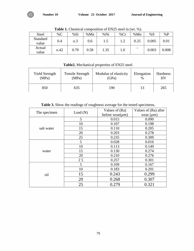
Journal of Engineering Volume 23 October 2017 Number 10
79
Table 1. Chemical composition of EN25 steel in (wt. %).
Steel %C %Si %Mn %Ni %Cr %Mo %S %P
Standard
value 0.4 o.3 0.6 1.5 1.2 0.25 0.005 0.01
Actual
value o.42 0.79 0.58 1.35 1.0
- 0.003 0.008
Table2. Mechanical properties of EN25 steel.
Table 3. Show the readings of roughness average for the tested specimens.
The specimen Load (N) Values of (Ra)
before wear( )
Values of (Ra) after
wear ( )
salt water
5 0.015 0.090
10 0.107 0.198
15 0.110 0.205
20 0.203 0.278
25 0.235 0.309
water
5 0.028 0.016
10 0.113 0.149
15 0.130 0.274
20 0.210 0.276
2 5 0.257 0.301
oil
5 0.109 0.167
10 0.183 0.201
15 0.243 0.299
20 0.268 0.307
25 0.279 0.321
Yield Strength
(MPa)
Tensile Strength
(MPa)
Modulus of elasticity
(GPa)
Elongation
%
Hardness
HV
850 635 190 13 265
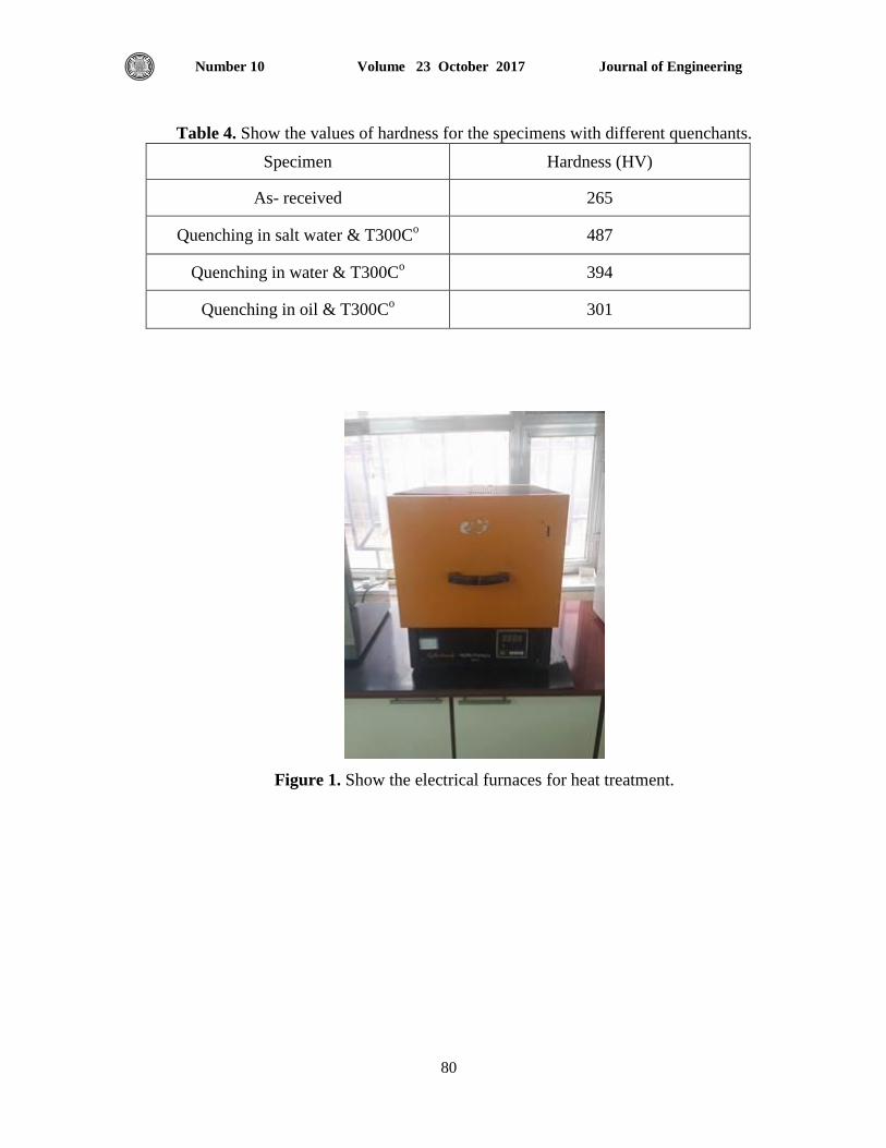
Journal of Engineering Volume 23 October 2017 Number 10
80
Table 4. Show the values of hardness for the specimens with different quenchants.
Specimen Hardness (HV)
As- received 265
Quenching in salt water & T300Co
487
Quenching in water & T300Co 394
Quenching in oil & T300Co 301
Figure 1. Show the electrical furnaces for heat treatment.
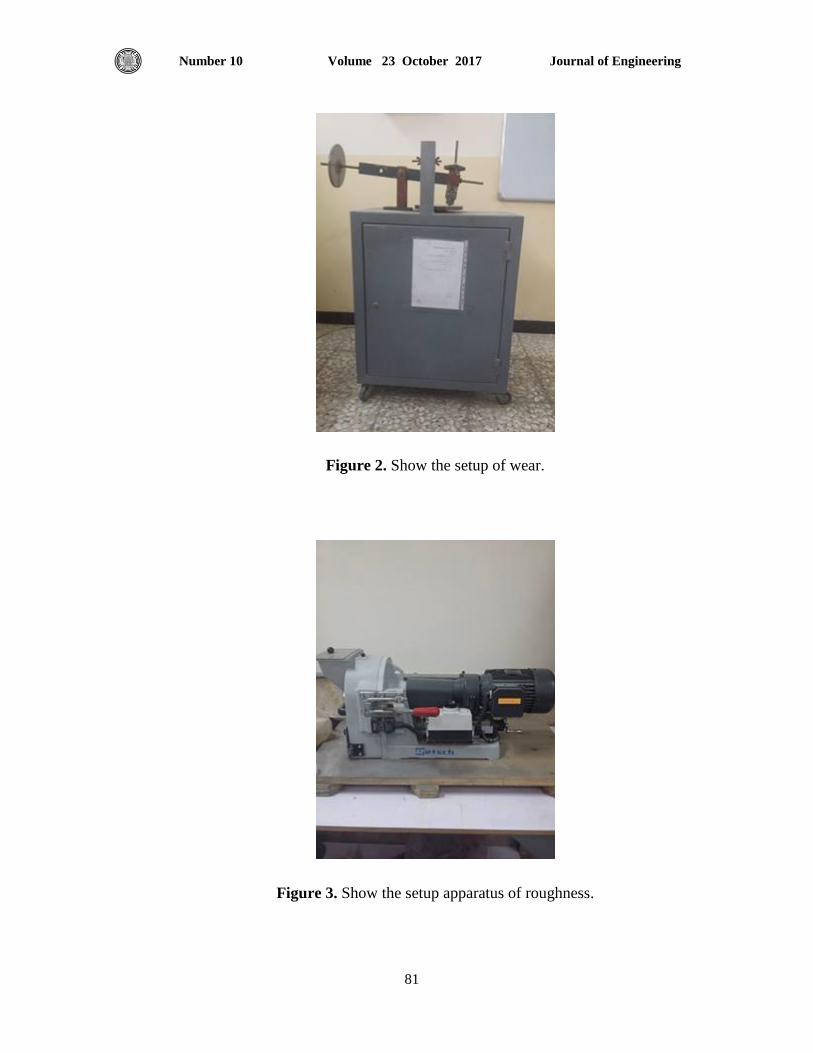
Journal of Engineering Volume 23 October 2017 Number 10
81
Figure 2. Show the setup of wear.
Figure 3. Show the setup apparatus of roughness.
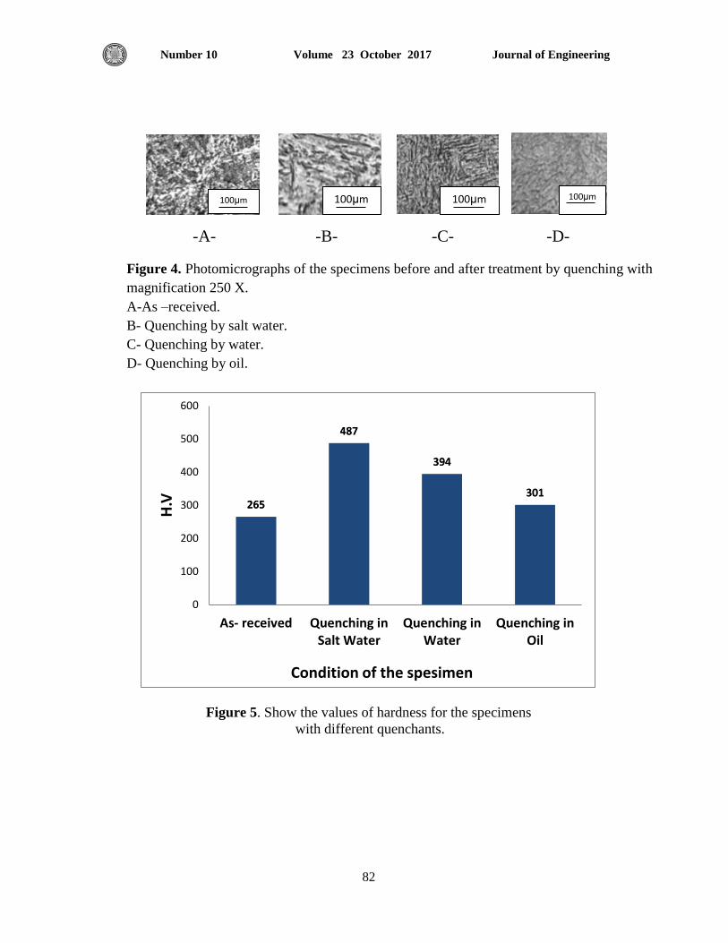
Journal of Engineering Volume 23 October 2017 Number 10
82
-A- -B- -C- -D-
Figure 4. Photomicrographs of the specimens before and after treatment by quenching with
magnification 250 X.
A-As –received.
B- Quenching by salt water.
C- Quenching by water.
D- Quenching by oil.
Figure 5. Show the values of hardness for the specimens
with different quenchants.
265
487
394
301 265
487
394
301
0
100
200
300
400
500
600
As- received Quenching inSalt Water
Quenching inWater
Quenching inOil
H.V
Condition of the spesimen
100µm 100µm 100µm
Table
100µm
Table
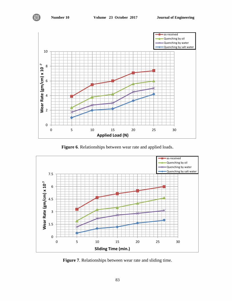
Journal of Engineering Volume 23 October 2017 Number 10
83
Figure 6. Relationships between wear rate and applied loads.
Figure 7. Relationships between wear rate and sliding time.
0
2
4
6
8
10
0 5 10 15 20 25 30
Wea
r R
ate
(gm
/cm
) x
10
-7
Applied Load (N)
as-received
Quenching by oil
Quenching by water
Quenching by salt water
0
1.5
3
4.5
6
7.5
0 5 10 15 20 25 30
Wea
r R
ate
(gm
/cm
) x
10
-7
Sliding Time (min.)
as-received
Quenching by oil
Quenching by water
Quenching by salt water

Journal of Engineering Volume 23 October 2017 Number 10
84
-A- -B- -C- -D-
Figure 8. Show the worn surfaces for the specimens treated by different quenchants before
and after wear test at load 15N.
A. As –received.
B. Quenching by salt water.
C. Quenching by water.
D. Quenching by oil.
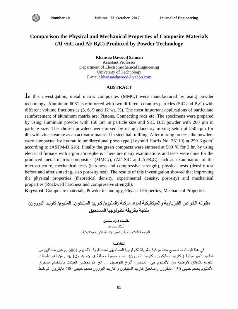
Journal of Engineering Volume 23 October 2017 Number 10
85
Comparison the Physical and Mechanical Properties of Composite Materials
(Al /SiC and Al/ B4C) Produced by Powder Technology
Khansaa Dawood Salman
Assistant Professor
Department of Electromechanical Engineering
University of Technology
E-mail: [email protected]
ABSTRACT
In this investigation, metal matrix composites (MMCs) were manufactured by using powder
technology. Aluminum 6061 is reinforced with two different ceramics particles (SiC and B4C) with
different volume fractions as (3, 6, 9 and 12 wt. %). The most important applications of particulate
reinforcement of aluminum matrix are: Pistons, Connecting rods etc. The specimens were prepared
by using aluminum powder with 150 µm in particle size and SiC, B4C powder with 200 µm in
particle size. The chosen powders were mixed by using planetary mixing setup at 250 rpm for
4hr.with zinc stearate as an activator material in steel ball milling. After mixing process the powders
were compacted by hydraulic unidirectional press type (Leybold Harris No. 36110) at 250 Kg/cm2
according to (ASTM-D 618). Finally the green compacts were sintered at 500 for 3 hr. by using
electrical furnace with argon atmosphere. There are many examinations and tests were done for the
produced metal matrix composites (MMCS), (Al/ SiC and Al/B4C) such as examination of the
microstructure, mechanical tests (hardness and compressive strength), physical tests (density test
before and after sintering, also porosity test). The results of this investigation showed that improving
the physical properties (theoretical density, experimental density, porosity) and mechanical
properties (Rockwell hardness and compressive strength).
Keyword: Composite materials, Powder technology, Physical Properties, Mechanical Properties.
(بيذ البورونرالمنيوم/ كاربيذ السليكون، المنيوم/ كا)مقارنة الخواص الفيزياوية والميكانيكية لمواد مركبة
منتجة بطريقة تكنولوجيا المساحيق
خنساء داود سلمان
أسخار هساػذ
لسن الهذست الكهشوهيكايكيت / الجاهؼت الخكىلىجيت
الخالصة
بىػيي هخخلفيي هي 6061في هزا البحث حن حظيغ هادة هشكبت بطشيمت حكىلىجيا الوساحيك. حوج حمىيت األلويىم
% . هي أهن حطبيماث 12، و9، 6، 3حجويت هخخلفت بسب (كاسبيذ السليكىى ، كاسبيذ البىسوى ) السيشاهيكيتالذلائك
الخمىيت بالذلائك ألسضيت هي األلويىم هي: الوكابس، أرسع الخىطيل . . الخ. حن ححضيش الؼياث بأسخخذام هسحىق
حن خلظ هايكشوى. 200كاسبيذ البىسوى بحجن حبيبي هايكشوى وهساحيك كاسبيذ السليكىى و 150األلويىم بحجن حبيبي
Journal of Engineering Volume 23 October 2017 Number 10
86
ساػاث هغ هادة سخشاث الزك كوادة 4دوسة / دليمت لوذة 250الوساحيك الوسخخذهت باسخخذام خالط كىكبي بسشػت
وليكي أحادي األحجا ىع بوكبس هيذس هشطت هغ كشاث طحي هي الفىالر. بؼذ ػوليت الخلظ حن حذهيج الوساحيك
(Leybold Harris No. 36110) كغن/ سن 250بومذاس2
(. أخيشآ حن حلبيذ ASTM-D 618بوىجب الوىاطفت )
م500جاث الخضشاء ػذ دسجت حشاسة الوذهo
ساػاث بأسخخذام فشى كهشبائي في جى هي اآلسكىى. أجشيج الؼذيذ 3لوذة
هثل فحض ( ألويىم / كاسبيذ السليكىى ، ألويىم/ كاسبيذ البىسوى )الوخجت والفحىطاث للوىاد الوشكبت هي األخخباساث
أجشي أخخباس الوساهيت. ث الكثافت لبل وبؼذ الخلبيذ، كزلكالبيت الوجهشيت ، أخخباساث الظالدة وهماوهت الضغظ، أخخباسا
( والخىاص الخجشيبيت، الوساهيت ، الكثافت )الكثافت الظشيت أظهشث خائج هزا البحث ححسي واضح في الخىاص الفيزياويت
الويكايكيت )طالدة سوكىيل، هماوهت األضغاط(.
حكىلىجيا الوساحيك، خىاص فيزيائيت، خىاص هيكايكيت. ،هشكبت هىاد: الكلمات الرئيسية
1. INTRODUCTION
In recent years an important researches were done to enhance the mechanical
properties of aluminum alloys by reinforcing them with ceramics particles such as SiC, B4C,
TiC and Al2O3, Zhenga, et al., 2014. Since the aluminum and its alloys have an attention as
an important metal to obtain metal matrix composites (MMCS) and more applications in
technology. To combine the light weight, corrosion resistance with mechanical properties
such as the strength, hardness and impact resistance leads to make the aluminum and its
alloys important matrix materials, Muthukrishnan, et al., 2008, Khairaldien, et al., 2008,
and Ahmed, et al., 2009. There are many reinforcement materials used for aluminum
matrix because of their strength are related with their particle size, the microstructure and
how they are distributed in the matrix which in turn improving the mechanical and physical
properties of the producing aluminum matrix composites, Attar, et al., 2015. Powder
metallurgy is an important technique using to obtain metal matrix composites with high
homogeneity more than for other methods, Nazik, et al., 2016. There are many researches
were published in this field like, Ekiki, et al., 2010. Investigated the effect of SiC and B4C
on the characteristics of the surface for the composites material. This study concluded that
there are many factors affected on the produced composites materials such as particle size,
volume fraction of the additive reinforced material. While Nagard, et al., 2013, studied the
effect of the addition of Al2O3 on the mechanical and wear behavior of the composites
materials of 6061 Al alloy metal matrix composites. The results of this work showed that the
wear resistance of B4C is lower than that of SiC particulate reinforcement of metal matrix
composites (MMCS). The aim of this work is to study the physical and mechanical properties
of metal matrix composites reinforced by two different of particulate reinforced materials
SiC and B4C for the matrix Al – 6061 alloy.
Journal of Engineering Volume 23 October 2017 Number 10
87
2. EXPERIMENTAL PROCEDURE
In this work, the composite materials Al/SiC and Al/ B4C are manufactured by using
powder technology as the following stages:
2.1 Preparing the Powders
The aluminum 6061 powder at 150 µm was in particle size, while the particulate
reinforcement SiC and B4C at 200µm in particle size. Table 1 shows the characteristics of
the powders used in this investigation.
2.2 Mixing the Powders
Two different composite materials were prepared by mixing the aluminum 6061
powders as a matrix at 150µm in the particle size with SiC and B4C as a reinforcement
material at 200µm in the particle size and adding zinc stearate as activator. Mixing process
was carried out by using planetary mixture as shown in Fig.1 with steel ball mill in 10 mm
diameter at 250 rpm for 3 hr.
2.3 Compacting Process
Compacting process for a mixture of the powders about 30gm in uniaxial hydraulic
press type (Leybold Harris No.36110), and then the mixed powders were pressed at 250 Kg/
cm2
in punch – die set assembly as shown in Fig.2. Inside die wall and the surface of punch
touch with the die were lubricated with graphite powder to prevent the green compacts from
adhesion with die wall and don’t crush during get out the die. The green compacts were
weighing by accuracy balance to calculate the density of them.
2.4 Sintering Process
Sintering process was done at 500 for 3 hr. in electrical furnace with inert atmosphere
(argon), sintering temperature increases with increasing the percentage of particulate
reinforcements to obtain the composites with high strength. After sintering, it must be to
calculate the density by divided the weight of the specimen to the volume.
2.5 Examinations and Tests
2.5.1 Microstructure examination
Microstructure examination of the Al/ Si and Al/ B4C composites were done by using
optical microscopy, before the examination of the microstructure, the specimens were cutting
and machined by lathe, and then grinded by grinding device with emery paper (500 and 1000)
µm in particle size. Following the grinding, the specimens were polished by polishing device
using diamond paste at size 0.7 µm for 30 min to obtain surfaces like mirror. Final stage for
preparing the composite specimens is etching them with 1% Keller reagent for 30 sec and then
washing with water before the examination for the microstructure.
Journal of Engineering Volume 23 October 2017 Number 10
88
2.5.2 Density test
Density test was carried out for the specimen before and after sintering. The differences in
values of density mean that there is porosity in the specimens. Porosity of the specimens before
and after sintering was calculated by using Archimedes formula.
The theoretical densities of metal matrix composites are measured by using the following
equation, Venkatesh, and Harish, 2015.
For Al/SiC
For Al/B4C
While the actual density after the sintering was calculated by using the following equation, Jain,
et al., 2016.
The porosity of the specimen was calculated by the following equation:
Porosity % 1
2.5.3 Hardness test
Hardness test was carried out for the specimens before and after sintering by using Rockwell
hardness equipment (Wilson Hardness machine, USA Model: LM 2481 T). Composites
specimens were tested by using (B) scale of Rockwell machine with hardened steel ball as an
indenter of 100 Kg were used for all the specimens. For each specimen, three readings were
taken at least and then determine the average of the three readings.
2.5.4 Compressive test
Compressive test was carried out for the specimens before and after sintering by using
Instron Universal Tester (type Instron 1195 machine with full capacity 2.5 ton). The specimens
were manufactured with 1.5 cm in height and 1 cm in diameter. All the specimens were
compressed at 1 ton until the specimen were crushed. Stress – Strain curve was plotted for each
composite material to obtain modulus of elasticity, yield strength and compressive strength.
Compression strength is calculated by the following formula:
Journal of Engineering Volume 23 October 2017 Number 10
89
3. RESULTS AND DISCUSION
3.1 Microstructure Analysis
The morphology of the sintered metal matrix composites was done by using optical
microscopy. SiC and B4C particulates were agglomerated in small volume fractions of them,
while increasing the volume fractions of SiC and B4C lead to make the particles to distribute
homogeneously in aluminum matrix and strong bonding was created between the particulate
reinforcement material and matrix as shown in Fig.3. As a result of compacting and
sintering, there are pores defects were obtained in the composites materials. During
sintering the particles of the mixing powders were joining together as a result of the welding
between them, also during sintering process, zinc stearate evaporated and then causes to
form porosity as a substitution of it is observed from Fig.4 that the increasing wt% of Sic
and B4C leads to increase % porosity, and then decreasing % porosity for SiC and B4C more
than 9% of them. It is perhaps at attributed to that the porosity acts as internal stresses at the
interfaces between the Sic, B4C particles and aluminum matrix.
3.2 Compacting and Sintering
The particulate reinforcement material increases the density during compacting and
sintering. Condensation occurs during compacting process and the particles close together with
increasing the pressing force, while during the sintering process as a result of thermal welding
between the particles, and then forming the necking between them which in turn causes the
shrinkage of the sintered specimens and in turn lead to improve the density which represents an
important of physical property, Khairaldien, et al., 2007. At the same time the temperature of
sintering process created a strong binding between the particulate reinforcement materials and
the matrix which affected on mechanical properties such as yield strength, ultimate tensile
strength and hardness because of the dispersion of particulate reinforcement materials in the
matrix, which causes a higher density of dislocation and make dislocation loop around a
reinforcement particles preventing them from any motion between them. Sun, et al., 2011, in
general, the density of composite material decreases with increasing the volume fraction of the
additive nanoparticles; it is attributed to that the decreasing of the wettability with increasing the
volume fraction of SiC, B4C and at the same time forming the pores at the interfaces between
SiC, B4C and the matrix, the density with SiC more than for B4C and also higher than for the
aluminum matrix. Fig.5 shows that obviously.
3.3 Effect of SiC and B4C on the Hardness of Composite Material
Mechanical properties of composite material dependent strongly on the volume fraction,
properties of the particulate reinforcement material, size of the additive particles. Increasing the
Journal of Engineering Volume 23 October 2017 Number 10
90
volume of SiC and B4C leads to increase the hardness of the manufactured of composite
manufactured of composite material. The hardness of composite material with SiC higher than
for composite material with B4C, it is return to that the SiC was made strong binding with
aluminum matrix higher than for B4C, also the particles of SiC prevent the dislocations and
pining them at their sites, and then increasing the hardness of the manufactured composite
material. This result is agreed with that of Jeevan, et al., 2012. Fig.6 shows that increasing the
volume fraction of SiC and B4C leads to increase the Rockwell hardness.
3.4 Effect of SiC and B4C on Compressive Strength
The compressive strength of a particle reinforced metal matrix composite is extremely
dependent on volume fraction of the additive particles and their sizes. Increasing the percentage
of SiC and B4C leads to increase the yield strength and compressive strength, it is attributed to
that the reaction between particles and the matrix which created thermal stresses because of the
differences between the melting point of SiC, B4C and aluminum as a matrix, and then in turn
increases the dislocation density. The reinforced particles obstacle the dislocation to move from
one particle to another and then increases the yield strength and compressive strength. Fig.7
shows that the increasing of volume fraction of SiC, B4C increases the compressive strength.
SiC increases the compressive strength more than B4C for the same reasons mentioned
previously. The result of this test is agreed with Shorowordi, et al., 2003.
4. CONCLUSIONS
Increasing the volume fractions of SiC and B4C for 6061 Al matrix leads to improve the
mechanical properties such as hardness and compressive strength.
1. Increasing the volume fractions of SiC and B4C for 6061 Al matrix leads to improve the
physical properties such as theoretical density, experimental density and porosity.
2. Small volume fractions of SiC and B4C were agglomerated in 6061 Al matrix, while
increasing the volume fractions of SiC and B4C were distributed homogeneously in 6061 Al
matrix, and the prefer percentage of SiC and B4C is (9%).
3. Improving the mechanical properties and physical properties for SiC more than for B4C.
Journal of Engineering Volume 23 October 2017 Number 10
91
5. REFRENCES
- Ahmed, A. R., Asokan, P., and Aravindan, S., 2009, EDM of hybrid Al-SiCP –GlassP
MMCS, International Journal of advanced manufacturing technology, Vol.44, No.5, , pp.520-
528.
- Attar, S., Nagaral, M., Reddapa, H. N., and Auradi, V., 2015, A review on particulate
reinforced aluminum metal matrix Composites, Journal of emerging technologies and
innovative research (JETIR), Vol. 2, Issue, pp.225-229.
- Callister, W. D., and JR., 2003, Material Science and Engineering, An Introduction, John
Wiely and Sons Inc., New York.
- Ekiki, R., Apalak, M. K., Yildirim, M., and Nair, F., 2010, Effect of random particle
dispersion and size on the indentation behavior of SiC particle reinforced metal matrix
composites, Materials and Design, Vol. 31, pp. 2818-2833.
- Jain, S., Rana, R. S., and Jain, P., 2016, Study of Microstructure and Mechanical
Properties of Al-Cu matrix reinforced with B4C particles Composite, International research
Journal of engineering and technology (IRJET), Vol.3, Issue. 1, pp 499-504.
- Jeevan, V., Rao, C.S., and Selvaraj, N., 2012, Compaction, sintering and mechanical
properties of Al-SiCp composites, International Journal of mechanical engineering and
technology (IJMET), Vol.3, Issue.3, pp. 565-573.
- Khairaldien, W. M., Khalil, A. A., and Bayoumi, M. R., 2007, Production of Aluminum-
Silicon Carbide Composites using Powder Metallurgy at sintering temperature above the
aluminum melting point, Journal of testing and evaluation, Vol. 35, No.6, pp. 111-125.
- Khairaldien,W.M., Khalil, A.A., Bayoumi, M.R., 2007, Production of aluminum-silicon
carbide composites using powder metallurgy at sintering temperatures above the aluminum
melting point, Journal of Testing and Evaluation. 35(6)111-125.
- Muthukrishnan, N., and Murugan, M., Rao, K. P., 2008, Machinability Issue in turning
Al-SiC (10%) metal matrix Composites, International Journal of advanced manufacturing
technology, Vol.17, No.3, pp. 1220-1228.
- Nazik, C., Tarakcioglu, N., Ozkaya, S., Erdemir, F., and Canakci, A., 2016, Determination
of effect of B4C content on Density and Tensile Strength of AA 7075/ B4C Composite
produced Via Powder Technology, International Journal of Materials, Mechanics and
Manufacturing, Vol.4, No.4, pp.251-254.
- Nagard, M., Bharath, V. and Auradi, V., 2013, Effect of Al2O3 particles on mechanical and
wear properties of 6061 Al alloy metal matrix composites, Journal of Material science and
Engineering, Vol. 2, No. 1, pp. 120-128.
Journal of Engineering Volume 23 October 2017 Number 10
92
- Sun, C., Song, M., Wang, Z., and He, Y, 2011, Effect of Particle Size on the
Microstructures and Mechanical Properties of SiC-Reinforced Pure Aluminum
Composites, Journal of Materials Engineering and Performance. 20(9) 1606-1612.
- Shorowordi, H.A., Laoui, T., Haseeb, A.S., Celis, I.P., and Froyen, L., 2003,
Microstructure and interface characteristics of B4C, SiC and Al2O3 reinforced Al matrix
composites: a comparative study, Journal of materials processing technology, Vol.14, pp.
738-743.
- Venkatesh, B., and Harish, B., 2015, Mechanical Properties of Metal Matrix Composites
(Al SiCP) particles produced by Powder Metallurgy, International Journal of Engineering
Research and General Science, Vol.3, Issue, pp. 1277-1284.
- Zhenga, R., chena, J., Zhanga, Y., and Mab, K. A., 2014, Fabrication and characterization
of hybrid structured Al alloy matrix coposites reinforced by high volume fraction of B4C
paticles, ELSEUIER, Materials Science and Engineering Al6061, pp20-28.
NOMENCLUTURE
d: diameter of the specimen(mm).
F: applied load (N).
h: height of the specimen(mm).
weight of the specimen in air (gm).
weight of the specimen in water (gm).
Al weight fraction of aluminum.
W SiC weight fraction of silicon carbide.
W B4C weight fraction of boron carbide.
c composite density (g /cm3).
Al density of aluminum (2.7 g/ cm3).
SiC density of silicon carbide (3.1 g/ cm3).
B4C density of boron carbide (2.51 g/ cm3).
: density of sintered specimen (gm/ cm3).
density of water (gm/ cm3).
s density of sintered specimen (gm/cm3).
th theoretical density of the specimen(gm/ cm3).
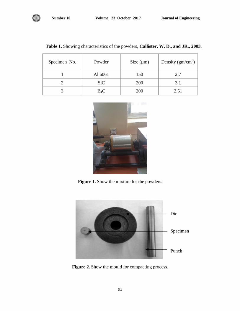
Journal of Engineering Volume 23 October 2017 Number 10
93
Table 1. Showing characteristics of the powders, Callister, W. D., and JR., 2003.
Specimen No. Powder Size (µm) Density (gm/cm3)
1 Al 6061 150 2.7
2 SiC 200 3.1
3 B4C 200 2.51
Figure 1. Show the mixture for the powders.
Figure 2. Show the mould for compacting process.
Specimen
Punch
Die
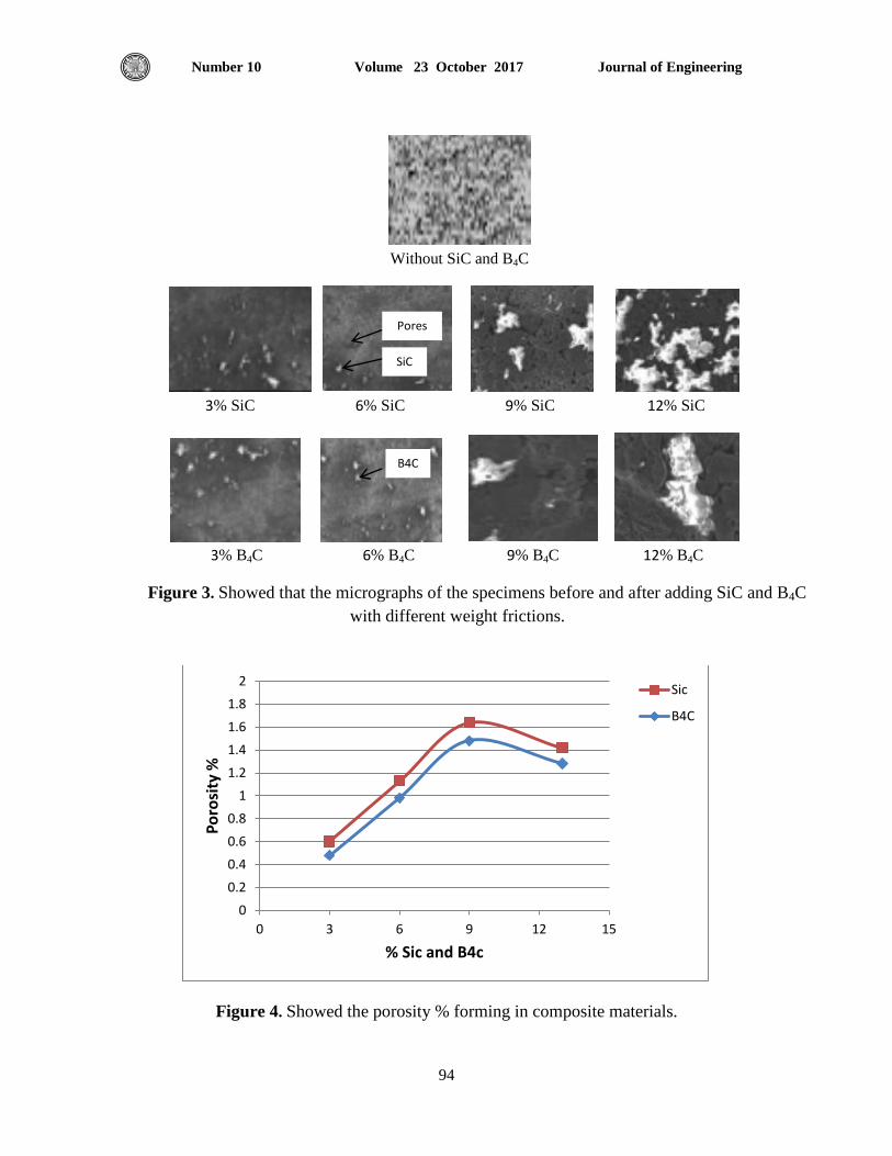
Journal of Engineering Volume 23 October 2017 Number 10
94
Figure 4. Showed the porosity % forming in composite materials.
0
0.2
0.4
0.6
0.8
1
1.2
1.4
1.6
1.8
2
0 3 6 9 12 15
Po
rosi
ty %
% Sic and B4c
Sic
B4C
Without SiC and B4C
3% SiC 6% SiC 9% SiC 12% SiC
3% B4C 6% B4C 9% B4C 12% B4C
Figure 3. Showed that the micrographs of the specimens before and after adding SiC and B4C
with different weight frictions.
Pores
SiC
B4C
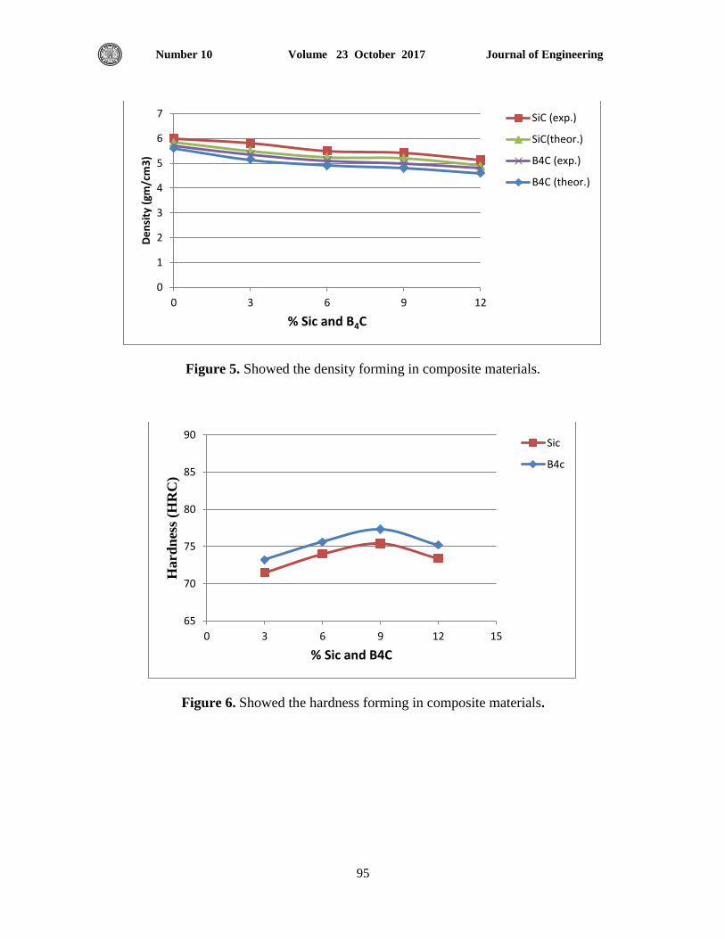
Journal of Engineering Volume 23 October 2017 Number 10
95
Figure 5. Showed the density forming in composite materials.
Figure 6. Showed the hardness forming in composite materials.
0
1
2
3
4
5
6
7
0 3 6 9 12
De
nsi
ty (
gm/c
m3
)
% Sic and B4C
SiC (exp.)
SiC(theor.)
B4C (exp.)
B4C (theor.)
65
70
75
80
85
90
0 3 6 9 12 15
Hard
nes
s (H
RC
)
% Sic and B4C
Sic
B4c
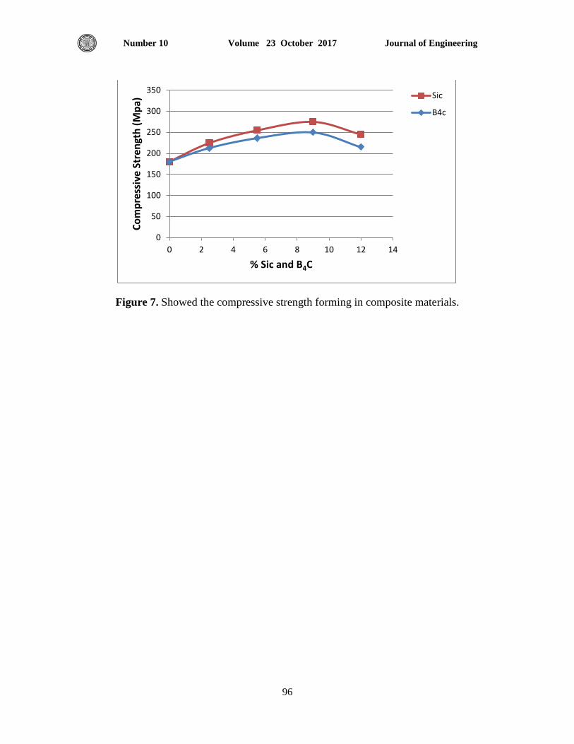
Journal of Engineering Volume 23 October 2017 Number 10
96
Figure 7. Showed the compressive strength forming in composite materials.
0
50
100
150
200
250
300
350
0 2 4 6 8 10 12 14
Co
mp
ress
ive
Stre
ngt
h (
Mp
a)
% Sic and B4C
Sic
B4c
Journal of Engineering Volume 23 October 2017 Number 10
:8
Bit Record Analysis for Bits Evaluating and Selection
Amel Habeeb Assi
Teacher assistant
College of Engineering - Baghdad University
E-mail: [email protected]
ABSTRACT
The bit record is a part from the daily drilling report which is contain information about the
type and the number of the bit that is used to drill the well, also contain data about the used
weight on bit WOB ,revolution per minute RPM , rate of penetration ROP, pump pressure
,footage drilled and bit dull grade. Generally we can say that the bit record is a rich brief about
the bit life in the hole. The main purpose of this research is to select the suitable bit to drill the
next oil wells because the right bit selection avoid us more than one problems, on the other hand,
the wrong bit selection cause more than one problem. Many methods are related to bit selection,
this research is familiar with four of those methods, which they are: specific energy method, bit
dullness way, cost per foot method, offset well bit record and geological information way. Five
oil wells have been studied in Rumaila Oil Field in South of Iraq which they are R-531, R-548,
R-536, R-544 and R-525. The wells R-531, R-536 and R-525 are vertical wells; the wells R-548
and R-544 are directional wells at angle of inclination 8.79◦ and 16.62
◦ respectively.
Key words: bit record, selection, bit, rate of penetration.
تحليل سجالث الحافرة من اجل تقييم اختيار الحافراث
امل حبيب عاصي
مدرس مساعد
جامعه بغداد–كليه الهندسه
الخالصت
لذي تضمن معلومات عن نوع وعدد وحجم الحافرات المستخدمة سجل الحافرة عبارة عن جزء من التقرر الوم للحفر واوتضمن سجل الحافرة اضا معلومات مهمة اخرى مثل مقدار الوزن المسلط على الحافرة ومقدار معدل .لحفر ذلك البئر
تضمن هذا دوران عمود الحفر ف الدققة الواحدة ومقدار معدل االختراق وعدد االقدام المحفورة وضغط المضخة واضا بعبارة اخرى مكن القول بان سجل الحافرة هو ملخص لحاة الحافرة السجل معدل تلف او تضرر الحافرة نتجة عملة الحفر.
الهدف الرئس من هذا البحث هو الختار الحافرات المناسبة لحفر االبار الجددة وذلك من .داخل الئر اثناء عملة الحفرالنه االختار الصحح لحافرة جنبنا الكثر من المشاكل اثناء الحفروالعكس البار نحفورة سابقا خالل تحلل سجل الحافرة
وطرقة كلفة حفر القدم لطاقة المحددة وطرقة تلف الحافرةمنها طرقة ا.توجد اكثر من طرقة الختار الحافرات صححثالثة من هذه قل الرملة جنوب العراق اخترت للدراسةف حابار 6 وطرقة سجل الحافرة والمعلومات الجلوجة. الواحد
. وتم حفر تلك االبار باستخدام انواع على التوال درجة 27773درجة و :978االبار عمودة واالخران موجهان بزاوت اختار الحافراتمادا على اسس طرق اعت ك الحافراتتقم ادائة تلتم مختلفة من الحافرات منتجة من ثالث شركات مختلفة و
سجل الحافرة,اختيار,حافرة,معدل االختراق7;الرئيست الكلماث
7

Journal of Engineering Volume 23 October 2017 Number 10
:9
1. INTRODUCTION All rig parts have one main purpose: to put a bit on the bottom of a hole and turn it to the right.
Rig owners and operators want a bit that gives a good rate of penetration. They also want the bit
to have longevity. The consideration that most affects bit selections the type of rock, or
formation, the bit must drill. Even though many types of formation exit, it is not practical for rig
operators to change bits every time. In this case, the rig operators would probably select a bit
designed to drill medium-soft rock or medium-hard. Manufactures make bits to drill various
formations hardness Bela, 2012. This research shows how to get benefit of the data from bit record to select the suitable bit for
drilling the next oil wells. These data belongs to five oil wells in south of Iraq. Since the bits that
drilled those sections didn't enter to the well and get out from it without any damaging, bit dull
grading is the window that from it, it can be known what happened to the bit that drilled those
depths. To get most footage and fastest penetration rate, and therefore the lowest cost, the
operator or contractor must choose the right bit for the job. Operators have several ways of
getting information to make this decision. Dull bit records from nearby wells show wear to the
bits used to drill them. For each well, the driller keeps a record of the depth, type of rock, fluids,
and anything else interesting about the operation. Bit record is helpful when drilling subsequent
wells in the same field. Aswad, 1996.
2. BIT SELECTION AND EVALUATION:
There is more than one way for choosing the best bit for drilling the oil wells, which they are:
1-specific energy way
2-bit dullness way
3- Offset well bit record and geological information way. Allen, 1980.
4-cost per foot way
The SE method depend on the minimum energy that is loosed at the bit to choose the bit, while
bit dull grade method depending on the degree of the dull characteristic that occurred at the bit
during drilling the well. A little bit damage mean good bit type and manufacturing and more bit
damaging, mean bad bit manufacturing and type. Generally, not the good bit manufacturing and
type effect on the bit dull grade, the drilling parameters, hydraulic and the type of formation, all
of them affect in great degree on bit dull grade. This study deals with all of pervious ways
Rabia ,1982 .Depending on available data, this research is interested with the all the above ways
of bit selection .
2.1 Specific Energy Method
The specific energy method gives an easy method for the suitable bits. It is defined as the
demanded energy to remove one unit volume from the drilled rock.it can be taken any
homogenous units. The equation of specific energy it can be derived by depending on the losses
force at the bit in one minute.so,
E=W*2
Where:
E: The mechanical energy, lb.-inch.
W: Weight on bit, lb.
N: Revolution per minute, RPM.
R: Radius of bit, inch.
The equation of raised rock volume in one minute is:

Journal of Engineering Volume 23 October 2017 Number 10
::
V= …………………………………………………………………………...2
Where:
PR: rate of penetration ft. /hr.
By dividing equation 1 and equation 2 to get the equation of specific energy
SE=E/V………………………………………………………………………………….3
SE= W*2 ……………………………………………………………..4
Where:
SE: Specific Energy,lb-inch/inch3
The equation of SE in lb-inch/inch3
units is:
SE=10 WN/R*ROP………………………………………………………………………5
By using the diameter of bit D in equation 5 instead of R where R=D/2, the equation 5
Will be:
SE=20 WN/D*ROP………………………………………………………………………6
From equation 6, it's clear that any changeable in the value of WOB and N lead to change in the
value of ROP, and that effect on the value of SE Rabia ,1985. It can be said that the SE method
represent direct measurement for bit performance for the formation to be drilled, also it is an
indicator to describe the interaction between the formation and the bit Harold J., 2013.
The value of SE don’t represent an essential properties of drilled rock, it is depend in great
degree on the bit design and type and manufacturing. The value of SE that result from drilling
soft formation different completely from the value of SE that result from drilling hard formation,
which mean the type of formation effect in great degree on the value of SE.it can be say that the
SE method is accurate method to select the suitable bit type. The more economical bit (optimum
bit), is the bit that give minimum value of SE R.Harmer , 2013.
Fig.1 shows the relation between the SE and the cumulative footage for three vertical oil wells
which they are: R-525, R-531 and R-536, the value of SE is calculated by using eq.6. The
columns 2, 3, 4 in Table 1,Table 2 and Table 3 represent the input data to get the column 4 in
those tables by using eq.6.
For the vertical oil wells, the following points are found:
1- The smith bit of GS105BVC model is the best bit to drill 17.5 " ,R-531 from 454.2 ft. to
1862.22 ft. hole section by depending on the SE method.
2- From 1862 ft. to 4287.6 ft., 12.25" hole section .Comparing with the other two wells, the
Baker H. Bit of HC606Z-PDC model in R-531 well is the best bit.
3- The Halliburton bit of SFD75H model that drilled 12.25 " hole section in R-536 well
from 4287 ft. to 5874 ft. is the best bit.
4- From 5874ft to 7358ft, 8.5"hole section in well R-531. Baker H. bit of Q506X-PDC
model gave the lowest value of SE.
Fig.2 Show the relation between the SE and the cumulative footage for tow directional oil
wells which they are: R-544 and R-548, the value of SE is calculated by using Eq. (6) ,the
column 2,3,4 in Table 4 and Table 5 represent the input data to get column 4 in those tables
by using Eq.(6):
For directional oil wells, the following points are found:
1- From 454ft to 1862 ft., 17.5"hole section in well R-548. Baker bit of GTX-CG1 model
gave the lowest SE value.
2- From 1862 ft. to 4000 ft., 12.25" hole section in well R-548. Baker bit of EP7199 model
gave the lowest SE value.
Journal of Engineering Volume 23 October 2017 Number 10
211
3- From 4000ft to 6510 ft., 12.25" hole section in well R-544. SMITH bit of MSI616LPX
model gave the lowest SE value.
4- From 6510 ft. to 7409ft 8.5" hole section in well R-544. Smith bit of MDi616LPX model
gave the lowest SE value. As we can see above, by using the SE method, it can be make
selection for the suitable bit to drill the next oil wells. The bits that gave the lowest values
of SE is the preferred bits. Fig. 3 show the relation between the SE and the cumulative
footage for all the studied oil wells
For the all (five oil wells), the following points are found:
1- The R-548 well gave the lowest value of SE compared with the other studied oil wells
for the 17.5"hole section.
2- The R-531 well gave the lowest value of SE compared with the other studied oil wells
for the 12.25 "hole section.
3- The R-531 well gave the lowest value of SE compared with the other studied oil wells
for the 8.5 "hole section.
2.2 Dull Bits Grading:
It is very important to grade dull bits properly. Grading a dull bit means estimating how much
and where it has worn. Proper dull bit grading helps the operator and the contractor correct poor
drilling practices, select the best type of bit for specific conditions, and make decisions that
affect the cost of future drilling. It is a form of ongoing field testing that benefits all drilling
contractors and operators Nollely, 1986. Roller cone bits and fixed –head (diamond) bits are both
graded using an International Association of Drilling Contractor (IADC) dull bit classification
system with eight categories as in Table 6 Since fixed-head bits have no bearing, the column for
bearing wear (B) always has an x in it when grading diamond bits. Roller con bits and fixed-head
bits use the same dull bit grading system. They are grading on the basis of cutter wear, bearing
wear (not for fixed-head), and gage wear Glowka, 1983.
Five wells have been studied each well consist of more than one section, the data that we have
belong to 17.5",12.25" and 8.5" hole sections for each well. Five wells mean five 17.5" hole
section and five 12.25" hole section and 8.5"hole section. Each section drilled by one bit or more
than one bit, that depend on if that the bit is good and able to drill the planed footage .sometimes
there are problems lead to use more than one bit. This study includes comparison each section in
each well with the other same section size for the other wells. The comparing between those
sections is about the degree of dullness to find the best bit from those bits to use it for drilling the
next oil wells.
Table 7 and Table 11 show that the 17.5"hole section in all studied wells drilled by using one
bit type because this hole section is not deep and the drilled footage not more than 600ft . Also,
the drilled formation in this hole section are Dibdiba, Lower Fars,Ghar,Dammam. The 17.5" hole
section is drilled by using milled teeth bits in many wells. The first part from 12.25"hole section
is drilled by using insert teeth bits and the second part is drilled by using PDC bits. The 8.5" hole
section is drilled by using PDC bits also.
Our data show that the 12.25" is drilled by using more than one bit type because the 12.25" hole
section is the longest drilled section compared with 17.5" and 8.5" hole section. From the other

Journal of Engineering Volume 23 October 2017 Number 10
212
hand the drilled formation in this hole section are Rus,UmmEr-
Radhuma,Tayarat,Shiranish,Hartha and Sadi . In the case of directional section, the bit which
drill vertical section differs from the bit which drill directional section because the directional
section is drilled by using PDC bit and different BHA than those which is used in vertical
section. The Roller cone bit (insert teeth bit or milled teeth bit) is just right for vertical section
only, but the PDC bit is used to drill directional section and vertical section. The drilling of
directional section needs special BHA like mud motor and Rotary Steerable System (RSS), PDC
bit can be run with those BHA. Table 12 and Table 13 contain more details about the bits that
was used to drill the studied oil wells.
The 12.25" hole size is drilled by using tow bit type in R-525 well and three bit in R-531well
and tow bit in R-536 well and tow bit type in R-544 well and three bit in R-548 well. For the
well R-525 the first bit is MDi616 bit, it was pulled due to slow ROP, Calcite stringer
interbedded at top of Tayarat may have been cause of damage, the second bit MDi616E Bit was
pulled at TD of 12 1/4" hole section. Bit was missing two cutters with three slightly chipped.
Smith Bit of model MDI616EPX was drilled 8.5"hole section in well R-525, the bit was in
relatively good condition, no chipped cutters, one nozzle lightly plugged, it can Rerun able to
drill other well. This bit is used to drill the 8.5"hole section in well R-548, and as in Table 9
Smith Bit of model MDI616EPX gave good bit dull grade, it can Rerun able to drill other well.
Depending on the degree of dull characteristic, the following points are found for vertical oil
wells and as in Tables 7, 8 and 9:
1- From 136 ft to 1566 ft, 17.5" hole section R-536 the Halliburton bit ofEBXT08SLCmodel
gave the lowest dull characteristic comparing with the others studied bits.
2- From 1696 ft to 4391 ft ,12.25" hole section R-525 Smith bit of MDi616 model gave the
lowest dull characteristic comparing with the others studied bits.
3- From 4420 ft to 5723 ft ,12.25" hole section R-525 the Smith bit of MDi616Emodel gave the
lowest dull characteristic comparing with the others studied bits.
4- From 5739 ft to 7327ft, 8.5" hole section R-525 the Smith bit of MDI616EPX model gave the
lowest dull characteristic comparing with the others studied bits.
Depending on the degree of dull characteristic, the following points are found for directional oil
wells and as in Table 10 and Table 11:
1- From 136 ft. to 1566 ft., 17.5" hole section.R-544 and R-548 both of the bit have the same dull
characteristic. Both of them gave good dull grade.
2- From 1696 ft. to 4391 ft ,12.25" hole section R-544 Smith bit oGFS10BVCf model gave the
lowest dull characteristic comparing with the others studied bits.
3- From 4420 ft. to 5723 ft., 12.25" hole section R-544 the Smith bit of MSI616LPXmodel gave
the lowest dull characteristic comparing with the others studied bits.

Journal of Engineering Volume 23 October 2017 Number 10
213
4- From 5739 ft. to 7327 ft,8.5" hole section R-548the Smith bit of MDi616LEPX model gave
the lowest dull characteristic comparing with the others studied bits.
2.3 cost per foot method
The cost per foot method and as in Eq. depends on the cost of bit, the total drilled footage, trip
time and rotating time and neglected the effect on the WOB, RPM and ROP on the bit
selection.Eq.7 represent the cost per foot equation
CPF=CB+CR (T+tr)/F………………………………………………………………….. (7)
Where:
CPF: cost per foot $/ft.
CB: bit cost $.
CR: Rig cost $/hr.
T: Total rotating time hr.
tr: trip time hr., t= RIH time+ POOH time……………………………………………..(8)
F: Total footage drilled.
Table 14 illustrates the cost per foot for the 17.5" hole section for all the studied oil wells, from
this table it's clear that the bit that drill the 17.5" hole section in R-536 Well is the best bit
compared with the other studied oil wells. This bit gave the lowest CPF compared with the other
studied oil wells while the bit that drill R-544 well show the biggest cost per foot. Table 15
illustrates the cost per foot for the 8.5" hole section for all the studied oil wells, from this table
it's clear that the bit that drill the 17.5" hole section in R-531 Well is the best bit compared with
the other studied oil wells. This bit gave the lowest CPF compared with the other studied oil
wells while the bit that drill R-548 well show the biggest cost per foot.
Note: for the 12.25" hole section, we have no accurate data concerning to the bits price and trip
time, so the studying is related only for 17.5" and 8.5"hole sections.
3. COMPARISON BETWEEN THE METHODS OF BIT SELECTION
Selecting the right bits is easier when drilling additional oil wells in the field because the
operator knows what formations to expect and which bit drills them best. Many methods are
used for bit selection, each way of them depending on one parameter or tow and neglected the
other, so it is from important to make connection between those methods for the accurate bit
selection. Sometimes tow method select the same bit type. The SE method depends on the
following drilling parameters: WOB, RPM and ROP but neglected the effect cost per foot and as
in Eq.6. Depending on the SE method we have the following results: the bits that drill the well
R-531 is the best bits compared with the other studied wells for vertical oil wells and the bits that
drill the both of wells R-544 and R-548 for directional oil wells. Depending on the cost per foot
method the CPF method, the Halliburton bit of EBXT08SLC model in well R-536, 17.5" hole
section has the lowest CPF value compared with the other studied oil wells. Also, depending on
the cost per foot method the CPF method, the bit Baker of Q506X-PDC model in well R-531, 8.5"
hole section has the lowest CPF value compared with the other studied oil wells
Journal of Engineering Volume 23 October 2017 Number 10
214
It is from important to put describing to the bit dull characteristic that occurs through drilling the
oil wells to get the benefit from it and the bit that gave low bit dull grade, is the bit that will be
used to drill the next oil wells. The bit dull grade method depends on the degree of dull grade
that occurred on the bit during drilling. The bits that drill the will R-525 is the best bits compared
with the other studied wells for vertical oil wells. The bits that drill the will R-544 is the best bits
compared with the other studied wells for directional oil wells. Generally, it should be take all
the above methods in our consideration during bit selection, which will be treated with all
parameters and not one parameters and that the key for the right bit selection. In other words, it
should be make combination between those methods.
Table 16 and Table 17. show the comparison between SE method and bit dull grade method for
vertical oil wells and directional oil wells. It's clear that each of those methods of bit selection
preferred bit model differ from the other method because each method followed specific line
different from the other.
4. CONCLUSIONS
1- Halliburton bit of EBXT08SLC model that drilled 17.5" hole section in well R-536 is the best
bit from the studied wells( it is gave the lowest dull characteristic compared with the other
studied bit in this study), is the best bit to drill 17.5"hole section in Rumaila oil field depending
on the bit dull grade method . It's drilled about 501 m in 33 hr. Also. For the same section and
depending on the SE method, the Smith bit of GS105BVC model in well R-531 has the lowest
SE value compared with the other studied vertical oil wells.
2- For directional well, 17.5" hole section, Smith bit of well R-544 of GFS10BVC model gave
the good dull characteristic, for the same section the Baker H.in well R-548 of GTX-CG1 model
gave the lowest value of SE.
3- SMITH bit of MSI616LPX model which was drilled12.25" hole section (directional part) in
R-548 well and the same section in R-544 well. It's drilled about 200 ft. in well R-548 and 950 ft.
in well R-544 in 99.97 hr. It gave good dull grade .It is recommended to use this bit to drill
12.25"hole sections (directional part) in this field.
4- Smith Bit of model MDI616EPX which was drilled 8.5"hole section in well R-525 and the
same section in well R-548,its drilled about 447 ft. in well R-548and 443ft in well R-525 ,its
drilled about 980 ft. This bit gave good dull grade, it is recommended to use this bit to drill
8.5"hole sections in this field.
5- Depending on the cost per foot method the CPF method, Halliburton bit of EBXT08SLC
model in well R-536, 17.5" hole section has the lowest CPF value compared with the other
studied oil wells.
6- Depending on the cost per foot method the CPF method, Baker H. bit of Q506XPDC
model in well R-531, 8.5" hole section has the lowest CPF value compared with the other studied
oil wells.
Journal of Engineering Volume 23 October 2017 Number 10
215
NOMENCLATURES:
BHA= bottom hole assembly.
ROP= rate of penetration, ft. /sec.
RPM= revolution per minute, Rev. /min.
WOB= weight on bit, lb.
DMLR= daily Mud Logger Report.
POOH = pull out of hole.
PCD = polly crystalline diamond.
BT= broken teeth.
HC= heat checking.
CT= chipped cutter.
WT= worn teeth.
ER= erosion.
PN=plugged nozzle.
RIH=running in hole
REFRENCES
Allen, J.H., 1980, Bit selection guidelines in vertical and directional oil wells, Oil and Gas J.,
94.
Aswad, Z. A. R., 1996, Advanced Drilling Engineering, M. Sc. Course at University of
Baghdad, Petroleum Engineering Dept.
Bela Liptak, April 2012, Control for Drilling Oil and Gas Wells.
Glowka, D., Febuary.1983, Optimization of Bit Configurations, Soc. Pet. Eng. J. pp.21-32.
Harold J. Flanagan, 2013, The Effect of drilling parameters on the value of Rate of
Penetration.
Nollely, J.P. 1986, An Analysis of Hydrualic Factors Affecting the Rate of Penetration of
Drag- Type Rotary Bits , Drill and Prod Prac., API , Dallas 23.
R.Harmer June 2013, Improving Drilling Results with A real-time Performance Advisory
System, Schlumberger, World Oil.
Rabia H."Specific energy as a csitesion for drill performance prediction" ,Int.J.Rock
Mech.Min Sci.19 ,No.1 Feb.(1982)
Rabia H."Oil well drilling engineering principles and practice" , Graham and Trotman
publishing Co.,(1985 )
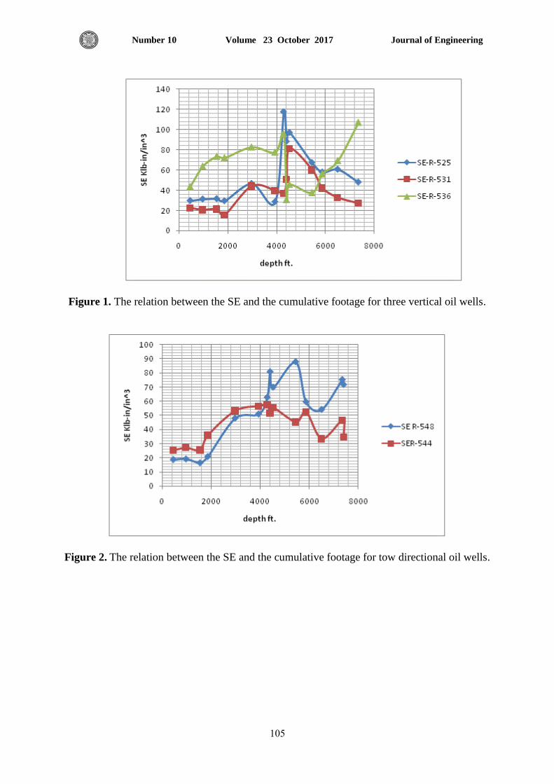
Journal of Engineering Volume 23 October 2017 Number 10
216
Figure 1. The relation between the SE and the cumulative footage for three vertical oil wells.
Figure 2. The relation between the SE and the cumulative footage for tow directional oil wells.
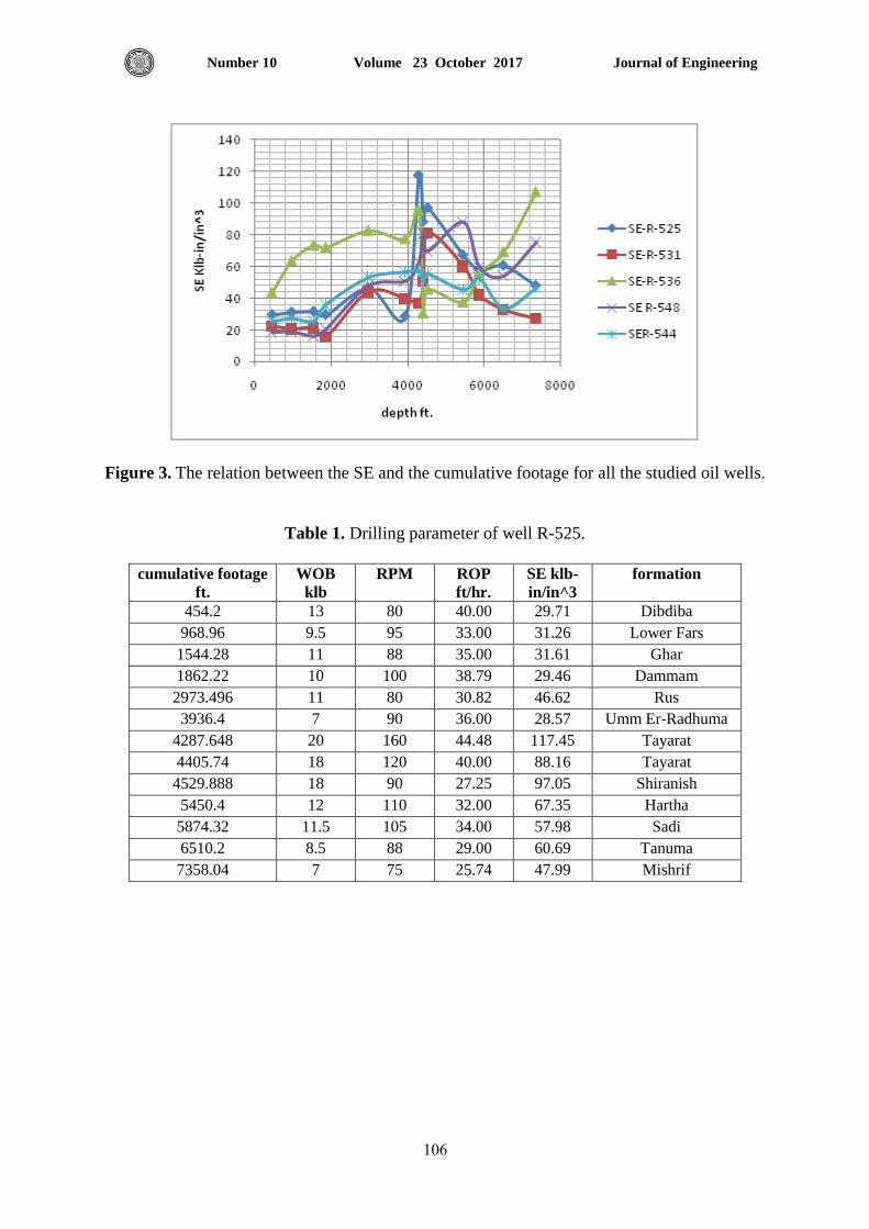
Journal of Engineering Volume 23 October 2017 Number 10
217
Figure 3. The relation between the SE and the cumulative footage for all the studied oil wells.
Table 1. Drilling parameter of well R-525.
cumulative footage
ft.
WOB
klb
RPM ROP
ft/hr.
SE klb-
in/in^3
formation
454.2 13 80 40.00 29.71 Dibdiba
968.96 9.5 95 33.00 31.26 Lower Fars
1544.28 11 88 35.00 31.61 Ghar
1862.22 10 100 38.79 29.46 Dammam
2973.496 11 80 30.82 46.62 Rus
3936.4 7 90 36.00 28.57 Umm Er-Radhuma
4287.648 20 160 44.48 117.45 Tayarat
4405.74 18 120 40.00 88.16 Tayarat
4529.888 18 90 27.25 97.05 Shiranish
5450.4 12 110 32.00 67.35 Hartha
5874.32 11.5 105 34.00 57.98 Sadi
6510.2 8.5 88 29.00 60.69 Tanuma
7358.04 7 75 25.74 47.99 Mishrif
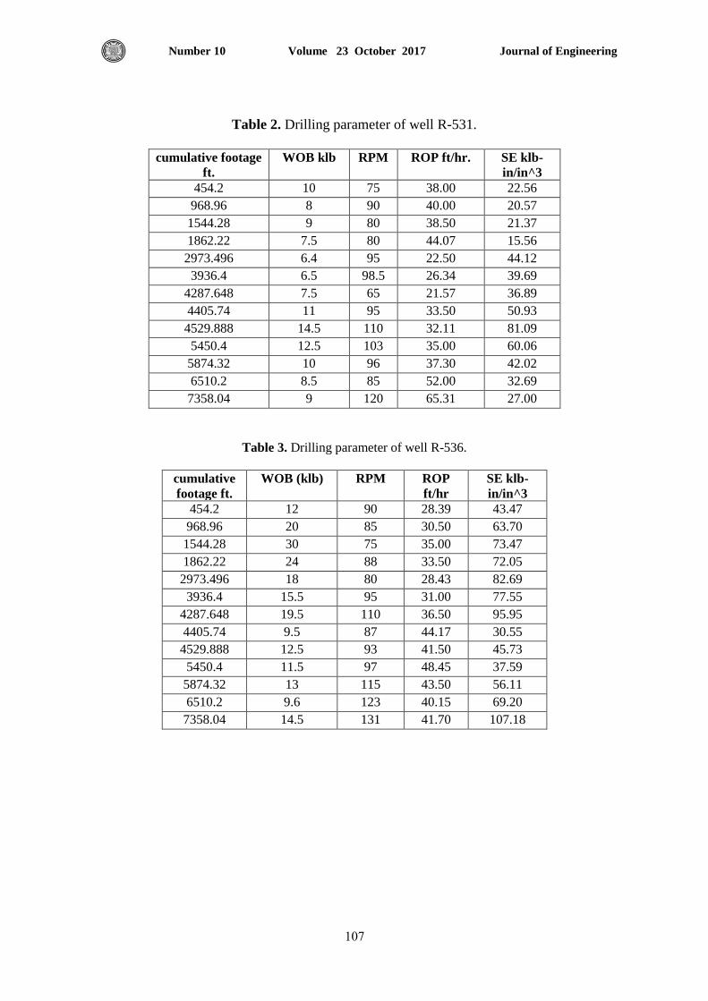
Journal of Engineering Volume 23 October 2017 Number 10
218
Table 2. Drilling parameter of well R-531.
cumulative footage
ft.
WOB klb RPM ROP ft/hr. SE klb-
in/in^3
454.2 10 75 38.00 22.56
968.96 8 90 40.00 20.57
1544.28 9 80 38.50 21.37
1862.22 7.5 80 44.07 15.56
2973.496 6.4 95 22.50 44.12
3936.4 6.5 98.5 26.34 39.69
4287.648 7.5 65 21.57 36.89
4405.74 11 95 33.50 50.93
4529.888 14.5 110 32.11 81.09
5450.4 12.5 103 35.00 60.06
5874.32 10 96 37.30 42.02
6510.2 8.5 85 52.00 32.69
7358.04 9 120 65.31 27.00
Table 3. Drilling parameter of well R-536.
cumulative
footage ft.
WOB (klb) RPM ROP
ft/hr
SE klb-
in/in^3
454.2 12 90 28.39 43.47
968.96 20 85 30.50 63.70
1544.28 30 75 35.00 73.47
1862.22 24 88 33.50 72.05
2973.496 18 80 28.43 82.69
3936.4 15.5 95 31.00 77.55
4287.648 19.5 110 36.50 95.95
4405.74 9.5 87 44.17 30.55
4529.888 12.5 93 41.50 45.73
5450.4 11.5 97 48.45 37.59
5874.32 13 115 43.50 56.11
6510.2 9.6 123 40.15 69.20
7358.04 14.5 131 41.70 107.18
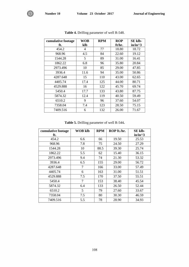
Journal of Engineering Volume 23 October 2017 Number 10
219
Table 4. Drilling parameter of well R-548.
cumulative footage
ft.
WOB
klb
RPM ROP
ft/hr.
SE klb-
in/in^3
454.2 4 77 18.80 18.72
968.96 4.5 84 22.60 19.12
1544.28 5 89 31.00 16.41
1862.22 6.8 96 35.80 20.84
2973.496 10 85 29.00 47.85
3936.4 11.6 94 35.00 50.86
4287.648 15 110 43.00 62.65
4405.74 17.4 125 44.00 80.71
4529.888 16 122 45.70 69.74
5450.4 17.7 133 43.80 87.75
5874.32 12.4 119 40.50 59.49
6510.2 9 96 37.60 54.07
7358.04 7.4 123 28.50 75.15
7409.516 6 132 26.00 71.67
Table 5. Drilling parameter of well R-544.
cumulative footage
ft.
WOB klb RPM ROP ft./hr. SE klb-
in/in^3
454.2 6.6 66 19.50 25.53
968.96 7.8 75 24.50 27.29
1544.28 10 88.5 39.30 25.74
1862.22 5.5 62 15.40 36.15
2973.496 9.4 74 21.30 53.32
3936.4 6.5 155 29.00 56.72
4287.648 7 166 33.00 57.49
4405.74 6 163 31.00 51.51
4529.888 7.5 170 37.50 55.51
5450.4 7 153 38.40 45.54
5874.32 6.4 133 26.50 52.44
6510.2 5 79 27.60 33.67
7358.04 7.5 80 30.30 46.59
7409.516 5.5 78 28.90 34.93

Journal of Engineering Volume 23 October 2017 Number 10
21:
Table 6. IADC Bit Dull Grade.
IADC : Dull Bit Grading
Cutting structure Example of bit grading : 2, 4, BT, M, E, X, (CT,WO), DTF.
Inner Outer Dull Char LocationBearings seals Gauge Other dull char Reason pulled
1 2 3 4 5 6 7 8
1 - Inner cutting structure (All inner rows.) 4 - Location
2 - Outer cutting structure ( Gauge rows only.) Roller cone Fixed cutterIn columns 1 and 2 a linear scale of 0 ---> 8 is used to describe the condition of the cutting
structure according to the following guidelines for specific bit types. N- Nose row G - Gauge row C - Cone S - Shoulder
Steel toothed bits Measure of lost tooth height due to abrasion and / or damage M - Middle row A - All Rows N - Nose G - Guage
0 - No loss of tooth height State cone # or #'s I.e. 1, 2, or 3. T - Taper A - All areas
8 - Total loss of tooth
Insert bits Measures total cutting structure reduction of lost, worn, & or broken inserts 5 - Bearings and seals
0 - No lost worn and / or broken inserts Non sealed bearings Sealed bearings
8 - 0% of inserts and / or cutting structure remaining. A linear scale estimating bearing life is used E - Seals effective F - Seals failed
Fixed cutter bits Measure of lost tooth height due to abrasion and / or damage 0 = No life used ---> 8, 100% bearing life used N - Not able to grade X - Fixed cutter bit
0 - No lost, worn and / or broken cutting structure 6 - Gauge
8 - 100% of cutting structure lost, worn and / or broken x - in gauge 1/16 - 1/16" out of gauge 1/8 - 1/8" ut of gauge 3/16-3/16" out of gauge
3 - Dull characteristics 1/4 - 1/14" out of gauge 5/16 - 5/16" out of gauge 3/8 -3/8" out of gauge 7/16 - 7/16" out of gauge
Note: use only cutting structure related codes 1/2 - 1/2" out of gauge 9/16 - 9/16" out of gauge 5/8 - 5/8" out of gauge etc.
BC - Broken cone * LN - Lost nozzle 7 - Other dull characteristicsBF - Bond failure LT - Lost teeth and cutters Refer to column 3 codes
BT - Broken teeth and cutters OC - Off centre wear 8 - Reasons bit was pulled or run completedBU - Balled up bit PB - Pinched bit BHA- Change bottom hole assembly HR - Hours on bit
CC - Cracked cone * PN- Plugged nozzle or flow by areas DMF - Downhole motor failure LOG - Run logs
CD - Cone dragged * RG - Rounded gauge DTF - Downhole tool failure PP - Pump pressure
CI - Cone interference RO - Ring out DSF - Drill string failure PR - Penetration rate
CR - Cored SD - Shirttail damage DST - Drill stem test Rig - Rig repair
CT - Chipped Teeth & cutters SS - Shelf sharpening wear DP - Drill Plug TD - Total depth / casing depth
ER - Erosion TR - Cone tracking CM - Condition mud TW - Twist off
FC - Flat crested wear WO - Wash out CP - Core point TQ - Torque
HC - Heat checking WT - Worn teeth or cutters FM - Formation change WC - Weather conditions
LD - Junk damage NO - No dull characteristics HP - Hole problems
LC - Lost cone * * Show cone # or #'s under location 4 LIH - Left in hole
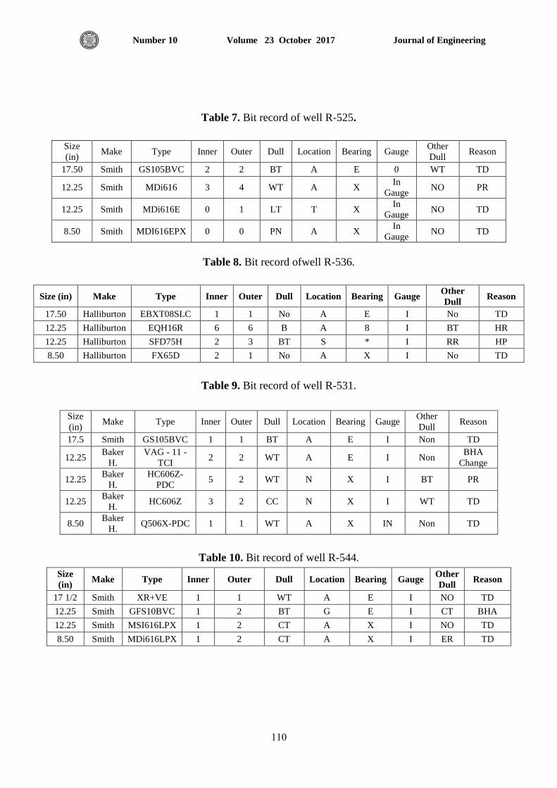
Journal of Engineering Volume 23 October 2017 Number 10
221
Table 7. Bit record of well R-525.
Size
(in) Make Type Inner Outer Dull Location Bearing Gauge
Other
Dull Reason
17.50 Smith GS105BVC 2 2 BT A E 0 WT TD
12.25 Smith MDi616 3 4 WT A X In
Gauge NO PR
12.25 Smith MDi616E 0 1 LT T X In
Gauge NO TD
8.50 Smith MDI616EPX 0 0 PN A X In
Gauge NO TD
Table 8. Bit record ofwell R-536.
Size (in) Make Type Inner Outer Dull Location Bearing Gauge Other
Dull Reason
17.50 Halliburton EBXT08SLC 1 1 No A E I No TD
12.25 Halliburton EQH16R 6 6 B A 8 I BT HR
12.25 Halliburton SFD75H 2 3 BT S * I RR HP
8.50 Halliburton FX65D 2 1 No A X I No TD
Table 9. Bit record of well R-531.
Size
(in) Make Type Inner Outer Dull Location Bearing Gauge
Other
Dull Reason
17.5 Smith GS105BVC 1 1 BT A E I Non TD
12.25 Baker
H.
VAG - 11 -
TCI 2 2 WT A E I Non
BHA
Change
12.25 Baker
H.
HC606Z-
PDC 5 2 WT N X I BT PR
12.25 Baker
H. HC606Z 3 2 CC N X I WT TD
8.50 Baker
H. Q506X-PDC 1 1 WT A X IN Non TD
Table 10. Bit record of well R-544.
Size
(in) Make Type Inner Outer Dull Location Bearing Gauge
Other
Dull Reason
17 1/2 Smith XR+VE 1 1 WT A E I NO TD
12.25 Smith GFS10BVC 1 2 BT G E I CT BHA
12.25 Smith MSI616LPX 1 2 CT A X I NO TD
8.50 Smith MDi616LPX 1 2 CT A X I ER TD
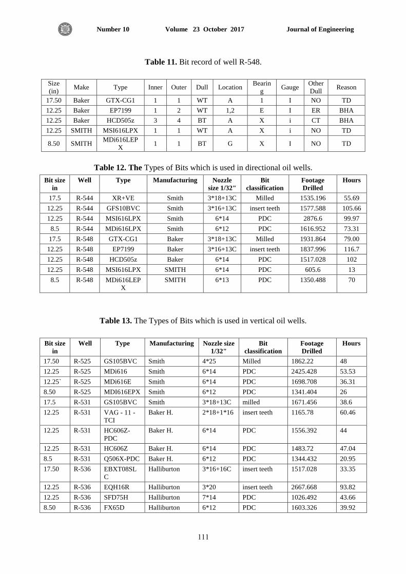
Journal of Engineering Volume 23 October 2017 Number 10
222
Table 11. Bit record of well R-548.
Size
(in) Make Type Inner Outer Dull Location
Bearin
g Gauge
Other
Dull Reason
17.50 Baker GTX-CG1 1 1 WT A 1 I NO TD
12.25 Baker EP7199 1 2 WT 1,2 E I ER BHA
12.25 Baker HCD505z 3 4 BT A X i CT BHA
12.25 SMITH MSI616LPX 1 1 WT A X i NO TD
8.50 SMITH MDi616LEP
X 1 1 BT G X I NO TD
Table 12. The Types of Bits which is used in directional oil wells.
Bit size
in
Well Type Manufacturing Nozzle
size 1/32"
Bit
classification
Footage
Drilled
Hours
17.5 R-544 XR+VE Smith 3*18+13C Milled 1535.196 55.69
12.25 R-544 GFS10BVC Smith 3*16+13C insert teeth 1577.588 105.66
12.25 R-544 MSI616LPX Smith 6*14 PDC 2876.6 99.97
8.5 R-544 MDi616LPX Smith 6*12 PDC 1616.952 73.31
17.5 R-548 GTX-CG1 Baker 3*18+13C Milled 1931.864 79.00
12.25 R-548 EP7199 Baker 3*16+13C insert teeth 1837.996 116.7
12.25 R-548 HCD505z Baker 6*14 PDC 1517.028 102
12.25 R-548 MSI616LPX SMITH 6*14 PDC 605.6 13
8.5 R-548 MDi616LEP
X
SMITH 6*13 PDC 1350.488 70
Table 13. The Types of Bits which is used in vertical oil wells.
Bit size
in
Well Type Manufacturing Nozzle size
1/32"
Bit
classification
Footage
Drilled
Hours
17.50 R-525 GS105BVC Smith 4*25 Milled 1862.22 48
12.25 R-525 MDi616 Smith 6*14 PDC 2425.428 53.53
12.25` R-525 MDi616E Smith 6*14 PDC 1698.708 36.31
8.50 R-525 MDI616EPX Smith 6*12 PDC 1341.404 26
17.5 R-531 GS105BVC Smith 3*18+13C milled 1671.456 38.6
12.25 R-531 VAG - 11 -
TCI
Baker H. 2*18+1*16 insert teeth 1165.78 60.46
12.25 R-531 HC606Z-
PDC
Baker H. 6*14 PDC 1556.392 44
12.25 R-531 HC606Z Baker H. 6*14 PDC 1483.72 47.04
8.5 R-531 Q506X-PDC Baker H. 6*12 PDC 1344.432 20.95
17.50 R-536 EBXT08SL
C
Halliburton 3*16+16C insert teeth 1517.028 33.35
12.25 R-536 EQH16R Halliburton 3*20 insert teeth 2667.668 93.82
12.25 R-536 SFD75H Halliburton 7*14 PDC 1026.492 43.66
8.50 R-536 FX65D Halliburton 6*12 PDC 1603.326 39.92
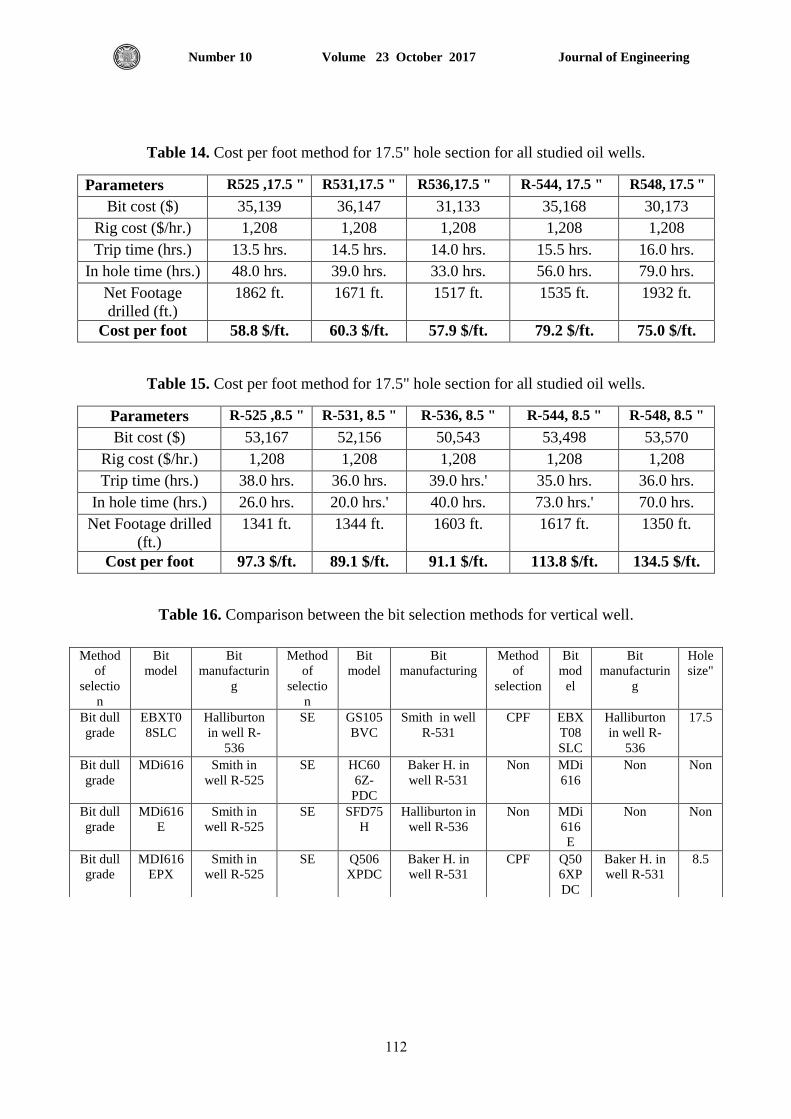
Journal of Engineering Volume 23 October 2017 Number 10
223
Table 14. Cost per foot method for 17.5" hole section for all studied oil wells.
Parameters R525 ,17.5 " R531,17.5 " R536,17.5 " R-544, 17.5 " R548, 17.5 "
Bit cost ($) 35,139 36,147 31,133 35,168 30,173
Rig cost ($/hr.) 1,208 1,208 1,208 1,208 1,208
Trip time (hrs.) 13.5 hrs. 14.5 hrs. 14.0 hrs. 15.5 hrs. 16.0 hrs.
In hole time (hrs.) 48.0 hrs. 39.0 hrs. 33.0 hrs. 56.0 hrs. 79.0 hrs.
Net Footage
drilled (ft.)
1862 ft. 1671 ft. 1517 ft. 1535 ft. 1932 ft.
Cost per foot 58.8 $/ft. 60.3 $/ft. 57.9 $/ft. 79.2 $/ft. 75.0 $/ft.
Table 15. Cost per foot method for 17.5" hole section for all studied oil wells.
Parameters R-525 ,8.5 " R-531, 8.5 " R-536, 8.5 " R-544, 8.5 " R-548, 8.5 "
Bit cost ($) 53,167 52,156 50,543 53,498 53,570
Rig cost ($/hr.) 1,208 1,208 1,208 1,208 1,208
Trip time (hrs.) 38.0 hrs. 36.0 hrs. 39.0 hrs.' 35.0 hrs. 36.0 hrs.
In hole time (hrs.) 26.0 hrs. 20.0 hrs.' 40.0 hrs. 73.0 hrs.' 70.0 hrs.
Net Footage drilled
(ft.)
1341 ft. 1344 ft. 1603 ft. 1617 ft. 1350 ft.
Cost per foot 97.3 $/ft. 89.1 $/ft. 91.1 $/ft. 113.8 $/ft. 134.5 $/ft.
Table 16. Comparison between the bit selection methods for vertical well.
Method
of
selectio
n
Bit
model
Bit
manufacturin
g
Method
of
selectio
n
Bit
model
Bit
manufacturing
Method
of
selection
Bit
mod
el
Bit
manufacturin
g
Hole
size"
Bit dull
grade
EBXT0
8SLC
Halliburton
in well R-
536
SE GS105
BVC
Smith in well
R-531
CPF EBX
T08
SLC
Halliburton
in well R-
536
17.5
Bit dull
grade
MDi616 Smith in
well R-525
SE HC60
6Z-
PDC
Baker H. in
well R-531
Non MDi
616
Non Non
Bit dull
grade
MDi616
E
Smith in
well R-525
SE SFD75
H
Halliburton in
well R-536
Non MDi
616
E
Non Non
Bit dull
grade
MDI616
EPX
Smith in
well R-525
SE Q506
XPDC
Baker H. in
well R-531
CPF Q50
6XP
DC
Baker H. in
well R-531
8.5

Journal of Engineering Volume 23 October 2017 Number 10
224
Table 17. Comparison between the SE method and bit dull grade method for directional wells.
Bit model Bit
manufacturing Method
of
selection
Bit model Bit
manufacturing Method
of
selection
Section
GFS10BVC Smith bit of
well R-544 Bit dull
grade GTX-CG1 Baker H.in
well R-548 SE 17.5
GFS10BVCf Smith bit of
well R-544 Bit dull
grade EP7199 Baker in well
R-548 SE 12.25
MSI616LPX Smith bit of
well R-548 Bit dull
grade MSI616LPX SMITH in
well R-544. SE 12.25
MDi616LEPX Smith bit of
well R-548 Bit dull
grade MDi616LPX . Smith bit of
well R-544 SE 8.5
Journal of Engineering Volume 23 October 2017 Number 10
114
Strength of Reinforced Concrete Columns with Transverse Openings
Dr. Ihsan A.S. AL-Shaarbaf Dr. Abbas AbdulMajeed Allawi Nabeel H. AlSalim Assistant Professor Assistant Professor Lecturer
Civil Engineering Department Civil Engineering Department Civil Engineering Department
Al-Israa University College College of Engineering College of Engineering
University of Baghdad Babylon University
ABSTRACT
The present work is concerned with the investigation of the behavior and ultimate capacity of
axially loaded reinforced concrete columns in presence of transverse openings under axial load plus
uniaxial bending. The experimental program includes testing of twenty reinforced concrete columns
(150 × 150 × 700 mm) under concentric and eccentric load. Parameters considered include opening
size, load eccentricity and influence of the direction of load eccentricity with respect to the
longitudinal axis of the opening. Experimental results are discussed based on load – lateral mid
height deflection curves, load – longitudinal shortening behavior, ultimate load and failure modes. It
is found that when the direction of load eccentricity is parallel to the longitudinal axis of openings,
column behavior is more pronounced when than the direction is normal to the longitudinal axis of
openings.
Keywords: RC Columns, Transverse Openings, Load eccentricity, Ultimate Load.
تحمل األعمدة الخرسانية المسمحة ذات الفتحات المستعرضة
السالم عمي حسن نبيل .د .م عالوي المجيد عبد عباس .د.م.أ الشعرباف صائب عمي احسان .د.م.أ
المدنية الهندسة قسم المدنية الهندسة قسم المدنية الهندسة قسم
بابل جامعة/الهندسة كمية بغداد جامعة/الهندسة كمية الجامعة االسراء كمية
الخالصة
الفتحات بوجود محوريا المحممة المسمحة االعمدةالخرسانية تحمل وقابمية االنشائي السموك دراسة عمى يتركز الخالي البحث ان
عمودا عشرون فحص البحث هذا من العممي البرنامج يتضمن .االتجاه احادية والعزوم المحورية االحمال تاثير تحت مستعرض
حجم إعتمادها جرى التي األساسية المتغيرات تضمنت .(ممم700) وبطول (ممم 150×150) بابعاد مربع مقطع ذات مسمحا خرسانيا
أساس عمى الفحص نتائج نوقشت .لمفتحة الطولي المحور اتجاه الى بالنسبة لمحمل الالمركزية اتجاه وتاثير لمحمل الالمركزية ,الفتحة
النتائج من وجد .الفشل وأنماط األقصى والحمل الطولي القصر - الحمل وسموك العمود منتصف عند الجانبي الهطول - الحمل سموك
االتجاه يكون عندما افضل بصورة العمود تصرف يكون لمفتحة الطولي المحور التجاه موازية الحمل التمركزية يكون عندما العممية
.لمفتحة الطولي المحور عمى متعامد
.االقصى الحمل ,التحميل المركزية ,المستعرضة الفتحات ,المسمحة الخرسانية االعمدة :المفتاحية الكممات
Journal of Engineering Volume 23 October 2017 Number 10
115
INTRODUCTION
Transverse openings may present in reinforced concrete columns as access for services including
plumbing pipes and electrical conduits. The presence of these openings results in reduction of
strength and stiffness and of the columns. If the presence of such openings is negligible during the
design these stage, structural damage may occurred. Lotfy, 2013, conducted a nonlinear finite
element analysis on 21 reinforced concrete column specimens using, ANSYS, 2010, software
version 10 to study the strength loss due to presence of transverse holes in columns. The parameters
considered were dimensions, shapes and positions of the holes. A comparison between the available
experimental results and finite element analysis is presented. It was found that results and
conclusions may be useful for designers.
Hassan, Sarsam and Allawi , 2013, 2015, studied the behavior of reinforced concrete
columns under uniaxial and biaxial bending. Their works deal with strengthening of columns by
using carbon fiber reinforced polymer (CFRP). The experimental program includes testing of eight
reinforced concrete columns (150×150×500mm) tested under several load conditions. The
considered variables are the effect of both eccentricity and longitudinal reinforcement (Ø12mm or
Ø6mm). Test results are discussed based on lateral and longitudinal deflection behavior, ultimate
load and failure modes. The CFRP strengthening shows a complete change in the failure mode of
the columns. Also, they concluded that the effect of longitudinal reinforcement in the case of
uniaxial and biaxial bending is more effective for strengthened columns than for unconfined
columns.
The ACI building Code ACI 318-2014 stated that "Conduits and pipes, with their fittings,
embedded within a column shall not occupy more than 4% of the cross-sectional area on which
strength is calculated". Experimental tests dealing with the effect of presence of transverse openings
inside columns is arrived out in the present study to investigate the strength reduction for concentric
and eccentric loaded columns. Also, the influence of transverse openings on the behavior and mode
of failure of the tested columns is investigated.
Al-Sali , 2015, studied the behavior and the load carrying capacity of reinforced concrete
short columns having different types of transverse openings. The experimental program deals with
the ultimate strength of tested columns. The variables considered in the experimental work include
shapes of openings having the same opening ratio of 0.133. The tested columns have been also
analyzed using a nonlinear finite element model. An increase in the ultimate strength of about 2.06%
is achieved when single opening of 20 mm diameter is replaced by two symmetrical openings of 10
mm diameter each. Also, a decrease in the ultimate strength of about 2.88% and 5.97% is observed
when the single circular opening of 20 mm diameter is replaced by 20×20 mm square opening or
20×40 mm rectangular opening respectively.
EXPERIMENTAL PROGRAM
Column specimens having an overall height of 900 mm and a square cross section of (150
mm × 150 mm) are considered. The transverse openings are positioned at mid height of the columns
as shown in Fig. 1. The opening ratio is calculated as the projecting area of the opening at the
opening level (i.e. at mid height of column) divided by the column cross sectional area. Reinforcing
steel bars provided for all columns are 4Φ10 mm longitudinal, and hence, the steel ratiois 1.4%,
which lies within the ACI 318-14 Code limitations. The transverse closed bars are consisted of Φ6
mm @ 100 mm as shown in Fig. 2.
Journal of Engineering Volume 23 October 2017 Number 10
116
Test length is considered as the middle part of the column having a 700 mm height. The remaining
100 mm upper and lower parts of the column are positioned inside the upper and lower steel caps to
apply the moments at the ends as shown in Fig. 3. This configuration is adopted to prevent possible
failure at the ends. Also, the embedded ends help to stabilize the specimen throughout the testing
procedure.
IDENTIFICATION OF SPECIMENS
To identify test specimens with different sizes of openings and eccentricities direction, the
following designation system is suggested:
• Group numbering: The first character is used to identify the group number. C1 refers to
specimens of group A in which the eccentricity is applied in direction parallel to the
longitudinal axis of openings, and C2 refers to columns of group B in which eccentricity is
applied in direction normal to the longitudinal axis of openings.
• Opening Size: The second character is used to identify the size of opening. Ф0 refers to
columns without opening, Ф15 refers to opening of 15 mm diameter, Ф20 refers to opening of
20 mm diameter and Ф25 refers to opening of 25 mm diameter.
• Load eccentricity: The third character is used to specify the values of load eccentricity. E0
refers to axially loaded columns. 45 refer to 45 mm loading eccentricity and E120 refers to 120
mm loading eccentricity.
Table 1 gives specimens designation system and opening details.
MATERIALS PROPERTIES
For each group, three standard cylinders (100×200mm) were tested to obtain the compressive
strength (fc'), splitting tensile strength (fct) (ASTM standard C496) and static modulus of elasticity
(Ec) at 28 days (ASTM standard C469) and at time of testing using a universal testing machine. The
standard mechanical properties of hardened concrete are listed in Table 2.
For all columns, two sizes of steel reinforcing deformed bars were used. Bars of size (Ф10 mm)
were used as longitudinal reinforcement and bars of size (Ф6 mm) were used as closed stirrups.
Values for yield stress and ultimate strength are obtained according to ASTM standard A615
requirements for each bar size and are given in Table 3.
TESTING PROCEDURE
A. Steel Caps
According to the previous researches, a precise load eccentricity using is difficult to obtain.
Hadi , 2007, concluded that the position of the applied load was not accurate and the columns had a
tendency to break at the tested connection region. Therefore, eccentric loading was simulated by
designing a new steel end caps to allow the eccentric load to be accurately positioned prior to testing
of the circular columns. Ranger and Bisb , 2007, used steel collars (caps) to fix their tested columns
and to ensure stability and accurate eccentric loading during testing. In the present work, new two
Journal of Engineering Volume 23 October 2017 Number 10
117
loading end caps were designed and implemented. In case of eccentric loading, each loading cap
was consisted of four Ф20 mm holes at the base of the cap through which the threaded part of the
longitudinal reinforcement is passed to ensure adequate length of development. In addition, each
side of loading cap includes three M24 female threads with bolts. These bolts were used to fasten
the loading cap together with the column through the available four (5×100×148 mm) steel plates.
These plates were used to prevent the column from damaging when the M24 bolts are tightened to
the column specimen. Another two (5×150×150mm ) steel plates were used at the top and bottom of
the tested column before placing the loading caps to protect the column during the test and to
distribute the applied loading across column cross section. Fig. 4 shows the steel caps and Fig. 5
represents a schematic representation with details.
B. Measurements and Instrumentation
In case of concentrically loaded columns, axial deformation was recorded using two dial
gages at two opposite sides of specimen over a length of 700 mm as shown in Fig. 6. While for the
eccentrically loaded columns, three additional dial gages were used to monitor the lateral
displacement for each specimen. The location of these dial gages were at mid height and at 320 mm
above and below mid height.
The average reading of the upper and lower dial gages has been subtracted from the reading
of the middle dial gage to obtain the net lateral displacement. Also, the axial deformations were
recorded using three dial gages over a length of 700mm of the eccentric columns. These dial gages
were fixed to the steel caps at different locations as shown in Fig. 7.
Also, a linear variable differential transformer (LVDT) is used to measure the axial
displacement across the opening by fixing it at two points on the tension face of the specimen and
the data of LVDT is recorded for each stage of loading as shown in Fig. 8.
C. Supporting System
The stability of the columns during testing is the main difficulty especially in case of high
value of eccentricity. Therefore, a supporting system was designed to stabilize the specimens during
testing. This system is consisted of four bolts located at the top and the bottom ends in touch with
the caps by using steel balls located at the ends, Fig. 9.
The benefit of these steel balls is to assure that the supporting system does not influence the
carrying capacity of the column and to prevent the possible horizontal movement of specimen at
ends. In addition, this system allows movement of column inside the machine to achieve the precise
eccentricity and allows the longitudinal movement of specimen to occur.
D. Loading Technique
A new loading system has been developed to apply the precise eccentric loading. This system
comprised a steel shaft with half spherical hole at its end, Ф45 mm steel ball and (10×90×90 mm)
square plate with a sector of spherical hole located at its middle as shown in Fig. 10. The steel shaft
can moves vertically inside a steel ring which prevents the shaft from horizontal sliding during
loading as shown in Fig. 11.
Journal of Engineering Volume 23 October 2017 Number 10
118
The location of this ring is at the center of testing machine at upper and lower bases. This
technique ensures that the load has a fixed loading.
E. Testing Procedure of the Columns Specimens
The testing machine shown in Fig. 12 has a capacity of 2000 kN. The load was gradually applied
and at each increment loasing, readings were recorded. In the trial test, the column was loaded up to
failure. The recorded data was analyzed to ensure the working conditions of all the instrumentation
used and the safety of testing procedure. After performing the trial test, the scheduled tests were
carried out.
The testing procedure is summarized as follows:
• Locating the column specimens inside the lower cap and then the upper cap was placed; All the
bolts were properly fastened.
• Lifting the column to the slide steel base level then sliding it into the testing machine as shown
in Fig. 13.
• Releasing the bolts of the loading cap.
• Applying concentric force to insure full contact between column and loading caps and
tightening all the bolts, then the applied load is removed.
• By using the supporting system, the column moves horizontally until reaching the precise
required eccentricity.
• The longitudinal bars were tightened to the loading caps especially in cases of eccentric loading
that may undergo tension.
• Applying fixation load then all dial gages are fixed and initial reading were recorded.
• The load was gradually applied in increments. At each load increment, all readings were
acquired manually.
EXPERIMENTAL RESULTS
A. Ultimate Strength Results
A.1: Group A (Load eccentricity in the direction parallel to the longitudinal axis of openings)
Foe all columns of group A, experimental ultimate strength values are shown in Table 4. These
columns have been tested under axial compressive load or axial load with 45 mm and 120 mm
eccentricity values in the direction parallel to the longitudinal axis of opening. For tested columns of
this group, in which zero eccentricity and different opening ratios of (0.00%, 10.00%, 13.33%, and
16.67%) were used, a significant reduction in ultimate strength is noticed due to the significant
reduction in compression area. The percentage decrease in the ultimate strength compared to column
C1Ф0E0 (reference column) were 3.21%, 5.02% and 6.22% for columns C1Ф15E0, C1Ф20E0 and
C1Ф25E0 respectively.
For the tested columns of this group, in which 45 mm eccentricity was exist with the same
different opening ratios shown above (0.00%, 10.00%, 13.33%, and 16.67%), a significant reduction
in the ultimate strength is observed since the opening area is located within the compression zone
for column cross section which reduces the compression area. The low eccentricity ratio (e/h=0.3)
for these columns makes the compression failure mode to be the dominant mode and no yielding of
tension reinforcement was occurred. The percentage decrease in the ultimate strength compared to
Journal of Engineering Volume 23 October 2017 Number 10
119
column C1Ф0E45 (reference column) were 6.36%, 10.46% and 12.27% for columns C1Ф15E45,
C1Ф20E45 and C1Ф25E45 respectively.
For tested columns of this group, in which 120mm eccentricity was exist and different opening
ratios of (0.00%, 10.00%, 13.33%, and 16.67%),an insignificant reduction in the ultimate strength
is noticed due to the large eccentricity ratio (e/h=0.8). The cracks in these columns at the tension
face are formed and the effect of bending moment is more pronounced than the effect of the axial
compressive load. The percentage decrease in the ultimate strength compared to column C1Ф0E120
(reference column) were 1.51, 1.51and 2.14 for columns C1Ф15E120, C1Ф20E120 and
C1Ф25E120 respectively as shown in Fig. 14.
A.2 Group B (Load eccentricity in the direction normal to the longitudinal axis of openings)
For all columns of group B, experimental ultimate strength values are given in Table 4. These
columns were tested under axial compressive load with 45 mm and 120 mm eccentricity values in
the direction normal to the longitudinal axis of opening. For tested columns of this group, in which
45mm eccentricity was exist and different opening ratios of (0.00%, 10.00%, 13.33%, and 16.67%)
were used, an insignificant reduction in the ultimate strength is observed since the opening area is
not located within the compression zone of the column cross section as shown in Fig. 15.
The percentage decrease in the ultimate strength compared to column C3Ф0E45 (reference
column) are 0.44, 0.85 and 1.31 for columns C2Ф15E45, C2Ф20E45 and C2Ф25E45 respectively.
For tested columns of this group, in which 120mm eccentricity was exist and different opening
ratios of (0.00%, 10.00%, 13.33%, and 16.67%) were used, a relatively insignificant decrease in the
ultimate strength is noticed, as shown in Fig. 14. due to the large eccentricity ratio (e/h=0.8). The
cracks in these columns at the tension face are formed and the effect of the bending moment is more
pronounced than the effect of the axial compressive load.
B. Effect of Transverse Openings on the Load-Deflection Behavior
B.1: Concentrically Loaded Columns
The experimental behavior of load versus axial shortening behavior of the columns of group A, in
which 0.0 mm eccentricity is used, are presented in Fig. 16. It can be noticed that the effect of
presence of transverse openings are significant because of the total opening area lies within the
column compression zonea. Also, it is evident that the increase in the opening area causes a
reduction in the ultimate load and increases the deflection at the ultimate load level.
B.2 Eccentrically loaded columns
B.2.1 Load eccentricity equal to 45 mm
Figs. 17 to 22 illustrate the influence of the presence of transverse openings on the load versus
vertical deflection response of the columns and lateral mid-height deflection curves of columns of
group A and two in which 45 mm loading eccentricity is used. For tested columns of group A most
of opening area lies within the column compression area that leads to a reduction in the ultimate
load values in addition to an increase in deflection at ultimate load level. This is due to the reduction
in stiffness and moment of inertia of the columns as the opening area increases. Also, one can
conclude from Figs. 17 to 22 that the effect of eccentricity of loading in direction parallel to the
longitudinal axis of openings (specimens of group A) is more than that of the direction when it is
normal to the longitudinal axis of openings (specimens of group B). This is because the opening is
existed in compression zone in case of parallel direction of opening axis and loading eccentricity
while this not find in the other case.
Journal of Engineering Volume 23 October 2017 Number 10
120
B.2.2 Load Eccentricity Equal to 120 mm
Figs. 23 to 28 show the effect of the presence of transverse openings on the load versus vertical
deflection response of the columns and lateral mid-height deflection curves of columns of group A
and two in which 120 mm loading eccentricity is used. From these figures, it is clear that the
increase in transverse opening size has a negligible effect on the ultimate load capacity. However,
the increase in opening ratio affects deflection values at the ultimate load because the increase in
opening ratio leads to a reduction in column stiffness.
C. Effect of Eccentricity on the Behavior of Reinforced Concrete Columns with Transverse
Openings
To study the effect of eccentricity of loading on the response of reinforced concrete columns
having transverse openings, eight columns of group A and eight columns of group B were tested
with two values of e/h (0.3 and 0.8).
C.1 Group A (load eccentricity in the direction parallel to the longitudinal axis of openings)
For group A and for columns having zero opening ratio (solid columns), the behavior of specimen
C1Ф0E45 is compared with that of specimen C1Ф0E120 using the load versus vertical and lateral
mid-height deflections as shown in Fig. 29 and Fig. 30. The ratio of ultimate capacity of column
C1Ф0E120 to that of column C1Ф0E45 is 0.3.
For same group and for columns having 0.1 opening ratio, the behavior of specimen C1Ф15E45 is
compared with that of specimen C1Ф15E120 using the load versus vertical and lateral mid-height
deflections as shown in Fig. 31 and Fig. 32. The ratio of ultimate capacity of column C1Ф15E120
to that of column C1Ф15E45 is 0.32. For columns having 0.133 opening ratio, the behavior of
specimen C1Ф20E45 is compared with that of specimen C1Ф20E120 using the load versus vertical
and lateral mid-height deflections as shown in Fig. 33 and Fig. 34. The ratio of ultimate capacity of
column C1Ф20E120 to that of column C1Ф20E45 is 0.33.
Finally, for the same group and for columns having 0.167 opening ratio, the behavior of specimen
C1Ф25E45 is compared with that of specimen C1Ф25E120 using the load versus vertical and lateral
mid-height deflections as shown in Fig. 35 and Fig. 36. The ratio of ultimate capacity of column
C1Ф25E120 to that of column C1Ф25E45 is 0.33.
C.2 Group B (load eccentricity in the direction normal to the longitudinal axis of openings)
For group B and for columns having zero opening ratio (solid section), specimen C3Ф0E45 is
compared with specimen C3Ф0E120 using the load versus vertical and lateral mid-height
deflections as shown in Fig. 37 and Fig. 38. The ratio of ultimate capacity of column C3Ф0E120 to
that of column C3Ф0E45 is 0.287.
For the same group and for columns of 0.1 opening ratio, specimen C3Ф15E45 is compared with
specimen C3Ф15E120 using the load versus vertical and lateral mid-height deflections as shown in
Fig. 39 and Fig. 40. The ratio of ultimate capacity of column C3Ф15E120 to that of column
C3Ф15E45 is 0.288.
For columns having 0.133 opening ratio, specimen C3Ф20E45 is compared with specimen
C3Ф20E120 using the load versus vertical and lateral mid-height deflections as shown in Fig. 41
and Fig. 42. The ratio of ultimate capacity of specimen C3Ф20E120 to that of specimen C3Ф20E45
is 0.289.
Journal of Engineering Volume 23 October 2017 Number 10
121
Finally, for the same group and for columns of 0.167 opening ratio specimen C3Ф25E45 is
compared with specimen C3Ф25E120 using the load versus vertical and lateral mid-height
deflections as shown in Fig. 43 and Fig. 44. The ratio of ultimate load of column C3Ф25E120 with
respect to that obtained for column C3Ф25E45 is 0.290.
TEST OBSERVATIONS
Images of selected tested concentrically and eccentrically loaded columns of groups A and B are
shown through Figs. 45 to 50.
For all concentrically loaded columns shown in Figs. 45 and 46, one can noticed that the
appearance of vertical cracks in concrete cover at the middle third zone of the specimen was always
the first sign of failure and cracks in all specimens with opening were noticed. They were generated
in a diagonal direction around the openings and growth to concur with the vertical cracks then these
cracks spread rapidly after spalling of concrete cover. At this stage, the concrete core carries the
applied axial load due to the coupling confinement effect of ties and longitudinal bars.
Failure is occurred in a brittle and explosive manner, where the longitudinal bars buckled and a
crush occurred in concrete at section of the opening and this section was separated into two sliding
surfaces. For all loaded specimens with 45mm eccentricity shown in Figs. 47 and 48, it can be
noticed that crushing of concrete was observed on the compression face of the columns at the
middle third zone of the specimen and few number of horizontal cracks in this zone initiated at the
tension face of the column. Some of these cracks pass through the opening and progress starting
from tension to compression faces. At later stage, the concrete cover firstly spalled off followed by
buckling of the longitudinal bars and a loss of strength was immediately observed after reaching the
peak load.
For all loaded columns with 120mm eccentricity shown in Figs. 49 and 50, one can noticed that a
large number of distributed horizontal cracks occurred at the tension face along the column. Also,
these cracks extended to the side faces of tested column especially at the middle third of specimen
length. These cracks are wider than the cracks at loaded columns with 45mm eccentricity. At a later
stage, the strength of specimen stood constant after reaching the peak value with a rapid increase in
crack width at tension face. Then concrete cover spalled off at the compression face and a loss of
strength was immediately observed after the peak load is reached.
CONCLUSIONS
According to the experimental tests carried out in this research work, the following conclusions
can be drawn:
1. The presence of transverse openings in reinforced concrete columns reduces the ultimate load
strength. For columns subjected to pure compressive axial load, the experimental results showed
a reduction in ultimate strength ranging between 3.21% and 6.22%.
2. For columns in which the load eccentricity is applied in the direction parallel to the longitudinal
axis of opening and tested with eccentricity equal to 45mm (e/h=0.3), the experimental results
showed a reduction in strength ranging between 6.36% and 12.27%, while for eccentricity equal
to 120mm (e/h=0.8), the experimental results showed that insignificant reduction in ultimate
strength can occur.
3. The experimental results showed that insignificant reduction is occurred for both eccentricities 45
and 120 mm for columns in which the load eccentricity is applied in the direction normal to the
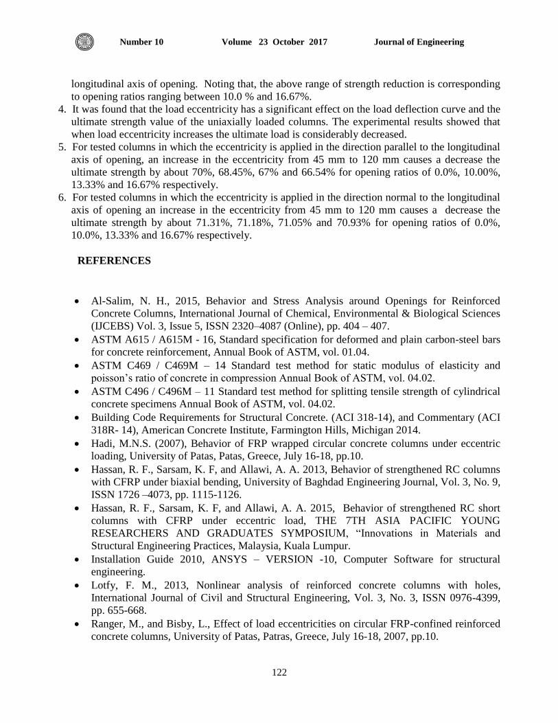
Journal of Engineering Volume 23 October 2017 Number 10
122
longitudinal axis of opening. Noting that, the above range of strength reduction is corresponding
to opening ratios ranging between 10.0 % and 16.67%.
4. It was found that the load eccentricity has a significant effect on the load deflection curve and the
ultimate strength value of the uniaxially loaded columns. The experimental results showed that
when load eccentricity increases the ultimate load is considerably decreased.
5. For tested columns in which the eccentricity is applied in the direction parallel to the longitudinal
axis of opening, an increase in the eccentricity from 45 mm to 120 mm causes a decrease the
ultimate strength by about 70%, 68.45%, 67% and 66.54% for opening ratios of 0.0%, 10.00%,
13.33% and 16.67% respectively.
6. For tested columns in which the eccentricity is applied in the direction normal to the longitudinal
axis of opening an increase in the eccentricity from 45 mm to 120 mm causes a decrease the
ultimate strength by about 71.31%, 71.18%, 71.05% and 70.93% for opening ratios of 0.0%,
10.0%, 13.33% and 16.67% respectively.
REFERENCES
Al-Salim, N. H., 2015, Behavior and Stress Analysis around Openings for Reinforced
Concrete Columns, International Journal of Chemical, Environmental & Biological Sciences
(IJCEBS) Vol. 3, Issue 5, ISSN 2320–4087 (Online), pp. 404 – 407.
ASTM A615 / A615M - 16, Standard specification for deformed and plain carbon-steel bars
for concrete reinforcement, Annual Book of ASTM, vol. 01.04.
ASTM C469 / C469M – 14 Standard test method for static modulus of elasticity and
poisson’s ratio of concrete in compression Annual Book of ASTM, vol. 04.02.
ASTM C496 / C496M – 11 Standard test method for splitting tensile strength of cylindrical
concrete specimens Annual Book of ASTM, vol. 04.02.
Building Code Requirements for Structural Concrete. (ACI 318-14), and Commentary (ACI
318R- 14), American Concrete Institute, Farmington Hills, Michigan 2014.
Hadi, M.N.S. (2007), Behavior of FRP wrapped circular concrete columns under eccentric
loading, University of Patas, Patas, Greece, July 16-18, pp.10.
Hassan, R. F., Sarsam, K. F, and Allawi, A. A. 2013, Behavior of strengthened RC columns
with CFRP under biaxial bending, University of Baghdad Engineering Journal, Vol. 3, No. 9,
ISSN 1726 –4073, pp. 1115-1126.
Hassan, R. F., Sarsam, K. F, and Allawi, A. A. 2015, Behavior of strengthened RC short
columns with CFRP under eccentric load, THE 7TH ASIA PACIFIC YOUNG
RESEARCHERS AND GRADUATES SYMPOSIUM, “Innovations in Materials and
Structural Engineering Practices, Malaysia, Kuala Lumpur.
Installation Guide 2010, ANSYS – VERSION -10, Computer Software for structural
engineering.
Lotfy, F. M., 2013, Nonlinear analysis of reinforced concrete columns with holes,
International Journal of Civil and Structural Engineering, Vol. 3, No. 3, ISSN 0976-4399,
pp. 655-668.
Ranger, M., and Bisby, L., Effect of load eccentricities on circular FRP-confined reinforced
concrete columns, University of Patas, Patras, Greece, July 16-18, 2007, pp.10.
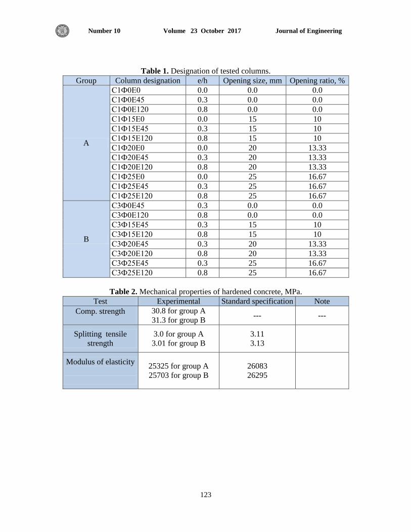
Journal of Engineering Volume 23 October 2017 Number 10
123
Table 1. Designation of tested columns.
Opening ratio, % Opening size, mm e/h Column designation Group
0.0 0.0 0.0 C1Ф0E0
A
0.0 0.0 0.3 C1Ф0E45
0.0 0.0 0.8 C1Ф0E120
10 15 0.0 C1Ф15E0
10 15 0.3 C1Ф15E45
10 15 0.8 C1Ф15E120
13.33 20 0.0 C1Ф20E0
13.33 20 0.3 C1Ф20E45
13.33 20 0.8 C1Ф20E120
16.67 25 0.0 C1Ф25E0
16.67 25 0.3 C1Ф25E45
16.67 25 0.8 C1Ф25E120
0.0 0.0 0.3 C3Ф0E45
B
0.0 0.0 0.8 C3Ф0E120
10 15 0.3 C3Ф15E45
10 15 0.8 C3Ф15E120
13.33 20 0.3 C3Ф20E45
13.33 20 0.8 C3Ф20E120
16.67 25 0.3 C3Ф25E45
16.67 25 0.8 C3Ф25E120
Table 2. Mechanical properties of hardened concrete, MPa.
Test Experimental Standard specification Note
Comp. strength
30.8 for group A
31.3 for group B --- ---
Splitting tensile
strength
3.0 for group A
3.01 for group B
3.11
3.13
Modulus of elasticity
25325 for group A
25703 for group B
26083
26295
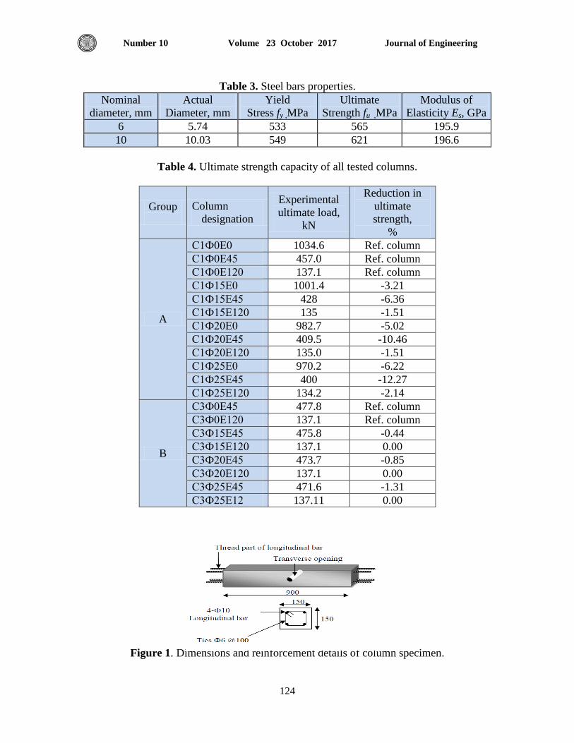
Journal of Engineering Volume 23 October 2017 Number 10
124
Table 3. Steel bars properties.
Nominal
diameter, mm
Actual
Diameter, mm
Yield
Stress fy ,MPa
Ultimate
Strength fu ,MPa
Modulus of
Elasticity Es, GPa
6 5.74 533 565 195.9
10 10.03 549 621 196.6
Table 4. Ultimate strength capacity of all tested columns.
Group
Column
designation
Experimental
ultimate load,
kN
Reduction in
ultimate
strength,
%
A
C1Ф0E0 1034.6 Ref. column
C1Ф0E45 457.0 Ref. column
C1Ф0E120 137.1 Ref. column
C1Ф15E0 1001.4 -3.21
C1Ф15E45 428 -6.36
C1Ф15E120 135 -1.51
C1Ф20E0 982.7 -5.02
C1Ф20E45 409.5 -10.46
C1Ф20E120 135.0 -1.51
C1Ф25E0 970.2 -6.22
C1Ф25E45 400 -12.27
C1Ф25E120 134.2 -2.14
B
C3Ф0E45 477.8 Ref. column
C3Ф0E120 137.1 Ref. column
C3Ф15E45 475.8 -0.44
C3Ф15E120 137.1 0.00
C3Ф20E45 473.7 -0.85
C3Ф20E120 137.1 0.00
C3Ф25E45 471.6 -1.31
C3Ф25E12 137.11 0.00
Figure 1. Dimensions and reinforcement details of column specimen.
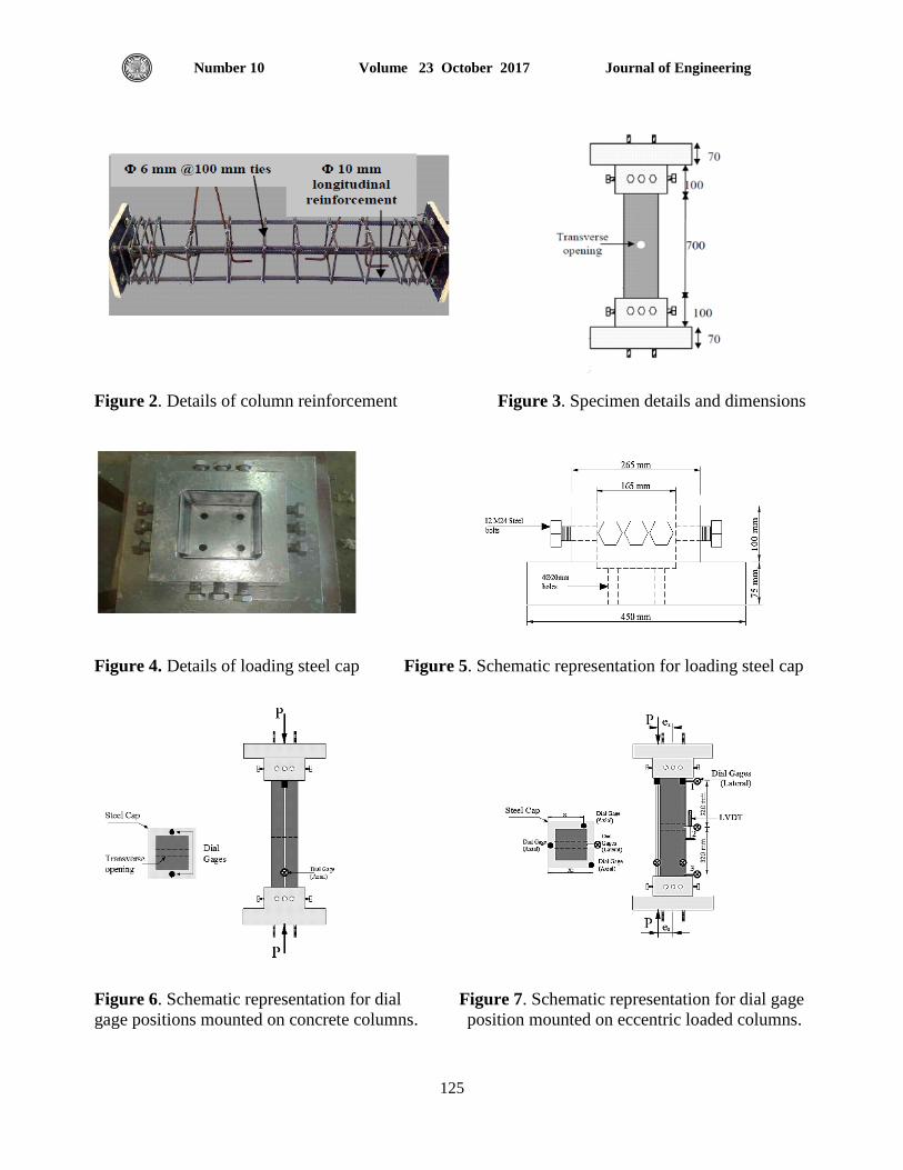
Journal of Engineering Volume 23 October 2017 Number 10
125
Figure 2. Details of column reinforcement Figure 3. Specimen details and dimensions
Figure 4. Details of loading steel cap Figure 5. Schematic representation for loading steel cap
Figure 6. Schematic representation for dial Figure 7. Schematic representation for dial gage
gage positions mounted on concrete columns. position mounted on eccentric loaded columns.
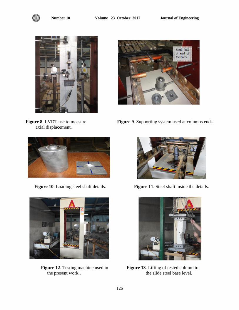
Journal of Engineering Volume 23 October 2017 Number 10
126
Figure 8. LVDT use to measure Figure 9. Supporting system used at columns ends.
axial displacement.
Figure 10. Loading steel shaft details. Figure 11. Steel shaft inside the details.
Figure 12. Testing machine used in Figure 13. Lifting of tested column to
the present work . the slide steel base level.
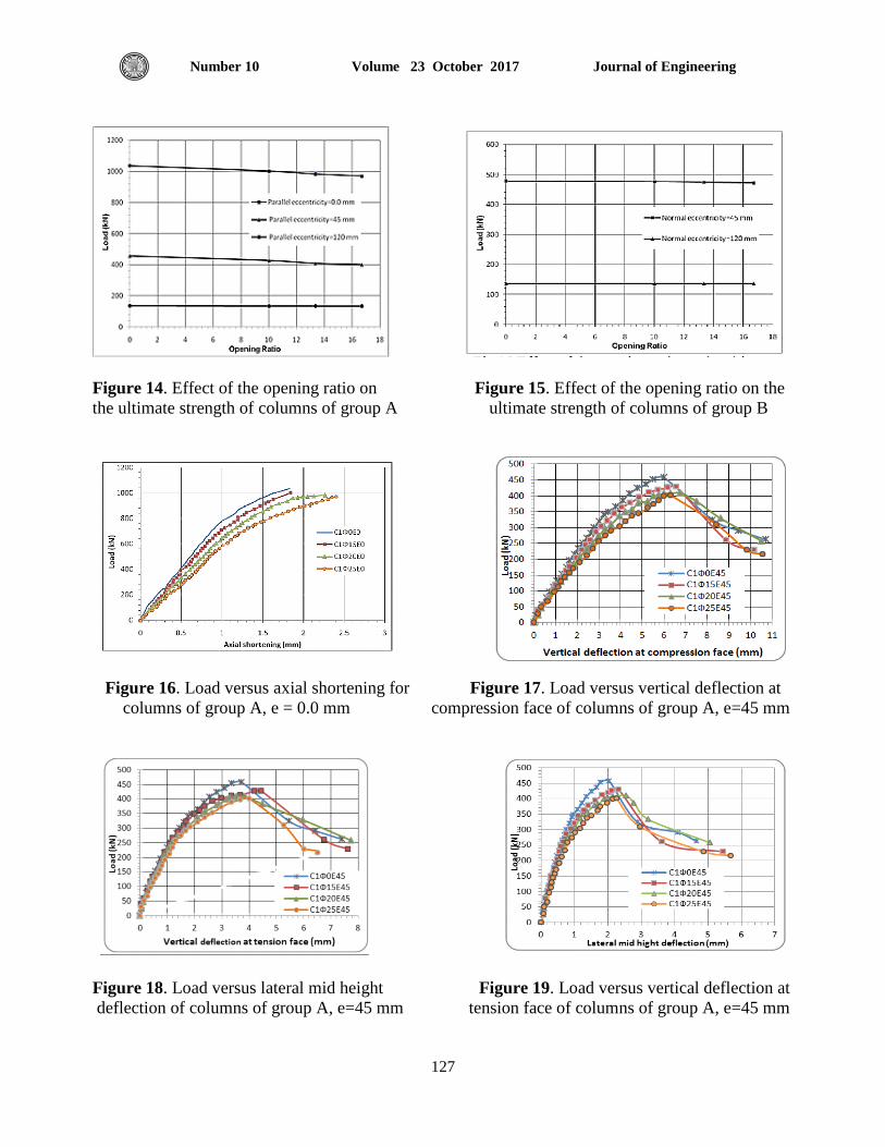
Journal of Engineering Volume 23 October 2017 Number 10
127
Figure 14. Effect of the opening ratio on Figure 15. Effect of the opening ratio on the
the ultimate strength of columns of group A ultimate strength of columns of group B
Figure 16. Load versus axial shortening for Figure 17. Load versus vertical deflection at
columns of group A, e = 0.0 mm compression face of columns of group A, e=45 mm
Figure 18. Load versus lateral mid height Figure 19. Load versus vertical deflection at
deflection of columns of group A, e=45 mm tension face of columns of group A, e=45 mm
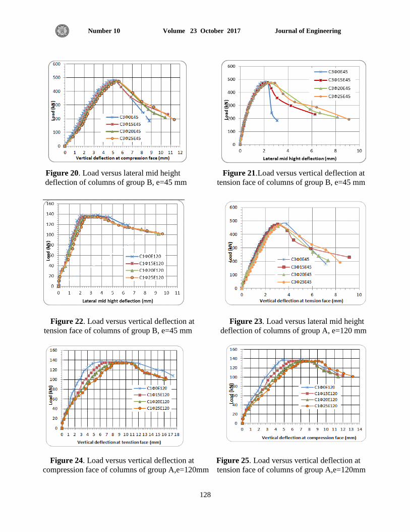
Journal of Engineering Volume 23 October 2017 Number 10
128
Figure 20. Load versus lateral mid height Figure 21.Load versus vertical deflection at
deflection of columns of group B, e=45 mm tension face of columns of group B, e=45 mm
Figure 22. Load versus vertical deflection at Figure 23. Load versus lateral mid height
tension face of columns of group B, e=45 mm deflection of columns of group A, e=120 mm
Figure 24. Load versus vertical deflection at Figure 25. Load versus vertical deflection at
compression face of columns of group A,e=120mm tension face of columns of group A,e=120mm
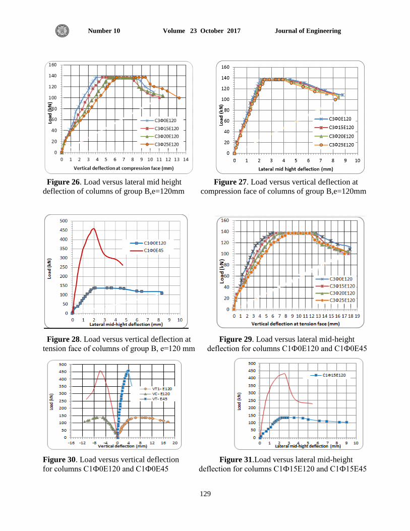
Journal of Engineering Volume 23 October 2017 Number 10
129
Figure 26. Load versus lateral mid height Figure 27. Load versus vertical deflection at
deflection of columns of group B,e=120mm compression face of columns of group B,e=120mm
Figure 28. Load versus vertical deflection at Figure 29. Load versus lateral mid-height
tension face of columns of group B, e=120 mm deflection for columns C1Ф0E120 and C1Ф0E45
Figure 30. Load versus vertical deflection Figure 31.Load versus lateral mid-height
for columns C1Ф0E120 and C1Ф0E45 deflection for columns C1Ф15E120 and C1Ф15E45
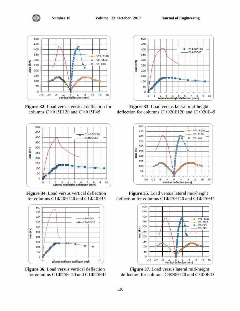
Journal of Engineering Volume 23 October 2017 Number 10
130
Figure 32. Load versus vertical deflection for Figure 33. Load versus lateral mid-height
columns C1Ф15E120 and C1Ф15E45 deflection for columns C1Ф20E120 and C1Ф20E45
Figure 34. Load versus vertical deflection Figure 35. Load versus lateral mid-height
for columns C1Ф20E120 and C1Ф20E45 deflection for columns C1Ф25E120 and C1Ф25E45
Figure 36. Load versus vertical deflection Figure 37. Load versus lateral mid-height
for columns C1Ф25E120 and C1Ф25E45 deflection for columns C3Ф0E120 and C3Ф0E45
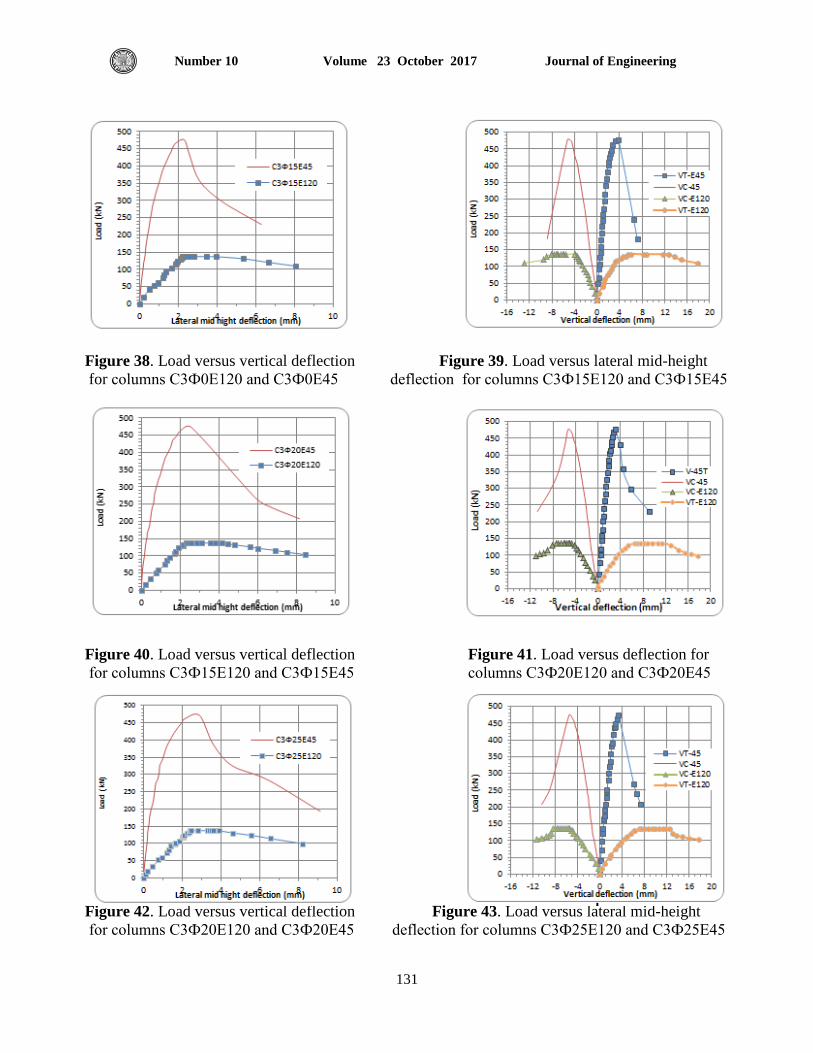
Journal of Engineering Volume 23 October 2017 Number 10
131
Figure 38. Load versus vertical deflection Figure 39. Load versus lateral mid-height
for columns C3Ф0E120 and C3Ф0E45 deflection for columns C3Ф15E120 and C3Ф15E45
Figure 40. Load versus vertical deflection Figure 41. Load versus deflection for
for columns C3Ф15E120 and C3Ф15E45 columns C3Ф20E120 and C3Ф20E45
Figure 42. Load versus vertical deflection Figure 43. Load versus lateral mid-height
for columns C3Ф20E120 and C3Ф20E45 deflection for columns C3Ф25E120 and C3Ф25E45
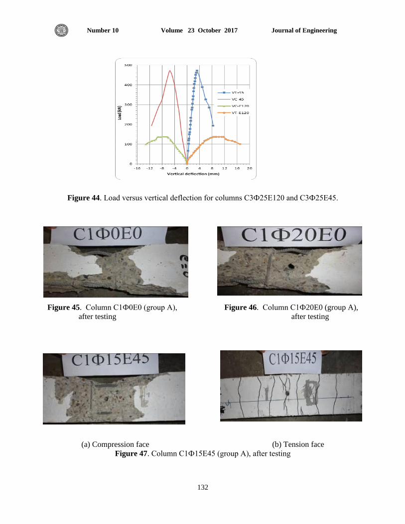
Journal of Engineering Volume 23 October 2017 Number 10
132
Figure 44. Load versus vertical deflection for columns C3Ф25E120 and C3Ф25E45.
Figure 45. Column C1Ф0E0 (group A), Figure 46. Column C1Ф20E0 (group A),
after testing after testing
(a) Compression face (b) Tension face
Figure 47. Column C1Ф15E45 (group A), after testing
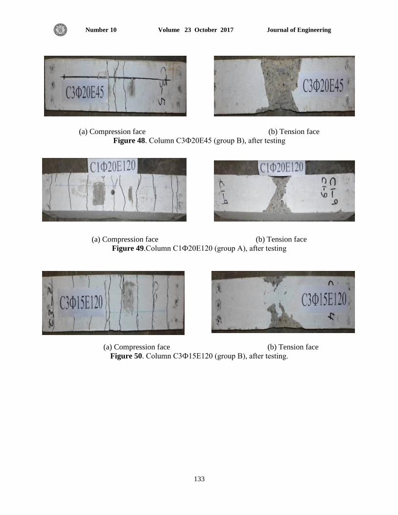
Journal of Engineering Volume 23 October 2017 Number 10
133
(a) Compression face (b) Tension face
Figure 48. Column C3Ф20E45 (group B), after testing
(a) Compression face (b) Tension face
Figure 49.Column C1Ф20E120 (group A), after testing
(a) Compression face (b) Tension face
Figure 50. Column C3Ф15E120 (group B), after testing.
Journal of Engineering Volume 23 October 2017 Number 10
431
Buckling Loads and Effective Length Factor for Non-Prismatic Columns
Taghreed Hassan Ibrahim
Assistant Lecture
Department of Civil Engineering
College of Engineering-University of Baghdad
E-mail: [email protected]
ABSTRACT
Based on a finite element analysis using Matlab coding, eigenvalue problem has been
formulated and solved for the buckling analysis of non-prismatic columns. Different numbers of
elements per column length have been used to assess the rate of convergence for the model. Then
the proposed model has been used to determine the critical buckling load factor ( ) for the
idealized supported columns based on the comparison of their buckling loads with the
corresponding hinge supported columns . Finally in this study the critical buckling factor ( ) under end force (P) increases by about 3.71% with the tapered ratio increment of 10% for
different end supported columns and the relationship between normalized critical load and
slenderness ratio was generalized.
Keywords: Buckling load, non-prismatic, finite element, eigenvalue.
نألعمدة غير انمنشوريتاالنبعاج ومعامم انطول انفعال أحمال
تغريد حسن إبراهيم
يذسط يساعذ
قسى انهنذسح انذنح
خايعح تغذاد –كهح انهنذسح
انخالصت
وحهها وفقا نرحهم انقح انزاذح يشكهح ذاو تشنايح اناذالب ذد صاغح تاالعراد عهى نظشح ذحهم انعناصش انحذدج وتاسرخ
طىل انعىد نرقى يعذل انرقاسب عهى ايرذادأعذاد يخرهفح ين انعناصش ذى اسرخذاواالنثعاج نألعذج غش اننشىسح.
ورنك نهقاسنح ألعذج يثانح اإلسناد ( ) االنثعاج انحشجنىرج األيثم. نقذ ذى اسرخذاو اننىرج انقرشح نرحذذ يعايم ــــــــنه
( ) انضادج نعايم االنثعاج انحشجوأخشا كاند .يع حانح اإلسناد انثسط تن أحال االنثعاج نحاالخ إسناد يخرهفح نألعذج
ونسثح % صادج ف نسثح انرذتة نخرهف حاالخ اإلسناد وكزنك ذى ذعى انعالقح تن انحم انحشج 41% نكم 37,4تحذود
عذج.اننحافه نال
انقح انزاذح.االنثعاج, غش ينشىسي, انعناصش غش انحذدج, حم انكهماث انرئيسيت:
1. INTRODUCTION
Determination of critical buckling load for elastic column is a key problem in engineering
design. Non-prismatic or tapered compression members are often used to achieve economy in
many practical applications, Shengmin, 1996. The first study on elastic stability is attributed to
Euler, 1744, who used the theory of calculus of variations to obtain the equilibrium equation and
buckling load of a compressed elastic column. Since many studies in this field have been made
such as Gere, et al., 1962, derived exact buckling solutions for many types of tapered columns
with simple boundary conditions. Ermopoulos, 1986 studied the buckling of the tapered
columns under axially concentrated loads at any position along the length direction for the
parabolically varying bending stiffness, Gere, et al., 1962. Groper, et al., 1987, developed a
method for predicting the critical buckling load for the particular case of concentrically loaded
Journal of Engineering Volume 23 October 2017 Number 10
431
columns with variations in cross-sectional area. Rzaiee, et al., 1995, used a geometrical
nonlinear analysis to solve non-prismatic or nonsymmetrical thin walled I-beam or columns, and
by using a computer program they generalized the results in form of design tables. Shengmin,
1996, used a modified matrix technique to study the elastic and inelastic buckling capacity of
non-prismatic members with a linear tapered I-shaped with a constant flange and a variable web.
Yossif, 2008, derived the elastic critical load of a non-prismatic member using the equations of
the modified stability functions for a wide range of taper ratio for rectangular or square cross
sectional shapes. Wei, et al., 2010, analyzed the buckling of prismatic and non-prismatic
rectangular columns under its weight and external axial force and discussed the influence of the
taper ratio on the critical buckling load. Al-Sadder, et al., 2004, determined an exact secant
stiffness matrix for a fixed-end forces vector for non-prismatic beam-column members under
tension and compression axial force.
2. THEORY
In the displacement field approach, a structure is usually dividing into a number of finite
elements and these elements are interconnecting at joints termed nodes as shown in Fig. 1. The
displacements within each element are represented by simple functions. The displacement
function is generally expressed in terms of a polynomial to be as or trigonometric function. For
a one dimensional idealization structure, the displacement field can be assumed in Eq. (1)[4]:
( )
( )
where:
( ) Is the displacement function at any x along the element.
a1, a2, a3 and a4 :Is the coefficients of the generalized coordinates.
In a matrix form, ( ) can be represented as;
⌊ ⌋ [
] ( )
The relation between the nodal degrees of freedom and the generalized coordinates can be
expressed in Eq.(3):
⌊ ⌋{a} ( )
and
⌊ ⌋ [
] ( )
Hence ; nodal displacements of an individual element will be expressed as:

Journal of Engineering Volume 23 October 2017 Number 10
431
[d]= [
] [
] [
]
or
[d]=[A]{a} ( )
then
{a}=, - * + ( )
Substitute Eq.(6) into Eq.(3) to get:
⌊ ⌋[A]-1
{d} ( )
Where:
[
]
( )
The total potential energy (∏p) for a member that subjected to an axial force (P) is expressed in
Eq. (9):
= strain energy + potential energy of applied force [2]
∫
(
)
∫
(
)
( )
This equivalent assumed that the potential of the loads is considered to be due to the forces
normal to the column length only. The summation of the two integrals of Eq. (9) is considered as
∏p=0.[4]
The term (.
/
) in the second integral expresses the strain due to rotation of the beam
element a length of ( (
)).
( )
, ( ) -
( )
Based on the above statements:
∫
∫
( )
Journal of Engineering Volume 23 October 2017 Number 10
43,
Where:
From Eq.(7) it will be get:
⌊ ⌋, - * + ( )
And noting that , , -
, -
⌊ ⌋ * + ( )
Where:
⌊ ⌋ ⌊ ⌋ , -
∫ * +
⌊ ⌋ ⌊ ⌋ * +
∫ * +
, - ⌊ ⌋ ⌊ ⌋ , - * + ( )
For a compressive force (P), we have
* + , -* +
* + [ ]* +
Let , - , - [ ]=Equivalent stiffness matrix for a beam element of combined axial and a
bending force actions.
Where:
, - ∫ ⌊ ⌋ ⌊ ⌋
( )
[Kg]=Geometric stiffness matrix
[ ] [ ]
[ ] ∫ , - ⌊ ⌋ ⌊ ⌋ , - * +
( )
[ ]
[
] ( )
The geometric stiffness matrix [ ] can be obtained by the consistent geometric stiffness
technique and the main advantage of this method that the eigenvalues were more accurate and
were proven upper bounds to the exact solution.
For the non-prismatic or tapered member we derived equation for the moment of inertia (Ix) of
the section at any distance (x) from the smallest end can be expressed in Eq. (17):

Journal of Engineering Volume 23 October 2017 Number 10
431
( )
( )
Where:
Io : Is the moment of inertia for the smallest section at x=0.
λ: Is the tapered ratio that represents the increasing in the moment of inertia so it’s defied as the
ratio of the moment of inertia at the bottom of the column I-section ( IL) to the moment of inertia
at the top of the column I-section (Io) as shown in Fig. 2.
Substitutes Eq. (17) into Eq. (14) and analytical integrated by Matlab software, an implicit form
has been derived for stiffness matrix [K].
Finally:
0, - [ ]1 * + * + ( )
For buckling problems: {F}= {0} , {D} ≠ {0} then
| |
Eigenvalue problems were solved by using the finite element method written in Matlb program.
The program used the element stiffness, mass matrix and modified the eigenvalue matrix
equation with given constraints. The modified eigenvalue matrix equation contained fictitious
zero eigenvalues in the same number of constraints. Finally solved this eigenvalue problem and
determine the critical buckling load factor ( ) for the lowest eignvalue. The critical buckling
load is expressed as shown in Eq. (19):
( )
3. CASE STUDIES:
A tapered I-section column of a constant flange width and linear increasing in the web depth was
adopted. It has a total length of (L) and under the effect of a concentrated axial load (P) on its top
as shown in Fig. 3.
For the columns shown in Fig. 3 there were different taper ratios (λ) of (1,1.1, 1.2, 1.3, 1.4, 1.5,
1.6, 1.7, 1.8, 1.9 and 2) with different boundary conditions of the hinged-hinged, clamped-free,
clamped-hinged and clamped-clamped end supported columns have been considered. Critical
buckling load factor ( ) for the case studies has been summarized in Table 1.
The following notations were used to describe column boundary conditions for different end
supports are summarized in Table 2.
4. VERIFICATION:
In order to investigate the validity of the results of the program we had to compare the buckling
load factor for linear tapered I-sections column for the tapered ratio of one only because of the
difference in the calculation of the studies for the tapered ratio where, Wei,2010, and Yossif,
2008, considered the tapered ratio as the ratio of width to length of a rectangular column section,
Journal of Engineering Volume 23 October 2017 Number 10
431
while in this study the tapered ratio is considered as the ratio of the moment of inertia at the
bottom to the top of the I-section, since the verification is used tapered ratio of one only and the
result was almost identical as shown in Table 3.
5. RESULTS AND DISCUSSIONS:
By using the finite element method in Matlab program to solve the eigenvlue problem in order to
compute the critical buckling load factor for the non-prismatic or tapered I-shape steel column
member, with linearly varied web height and with constant flange dimension.
Table 1 gave the critical buckling load factor ( cr) of the web tapered column under axial force
(P) acting at the top of the column for different boundary conditions. Different number of
elements (from 4 to 11) along column length gave results that are quite close with a relative error
not greater than (3%).
The results obtained from Table 1 showed that average increasing in tapered ratio leads to
increasing the buckling load factor about 4.17% for the hinged-hinged end supported column and
about 3.6% for the clamped-free, clamped-hinged and clamped-clamped end supported columns,
that mean for each 10% increase in the moment of inertia for the column section leads to average
increasing of 3.71% for the hinged-hinged, clamped-free, clamped-hinged and clamped-clamped
end supported columns.
To present the relationship between the normalized critical load defined by (Pcr/fy.A) and the
slenderness ratio (KL/r) as shown in Table 4 and Fig. 4, the hinged-hinged column end supports
was implemented with different tapered ratios of (1, 1.2, 1.4, 1.6, 1.8 and 2 ) and used the wide-
flange section of (W30x211) as shown in Table 5 to represents the section properties of the
radius of gyration (r), moment of inertia (I), and area of the section (A). The modulus of
elasticity (E) and the yield strength of steel (fy) were considered as (200 GPa) and (250 MPa)
respectively. The slenderness ratio was limited by the maximum short and intermediate column
limit (Cc) factor which calculate from the Eq.(20) and the maximum long column limit
(KL/r=200)[6].
√
( )
Convergence for the critical buckling factor for the case of hinged-hinged column end supports
could be obtained with three or more elements mesh as shown in Fig. 5.
6. CONCLUSIONS:
The buckling of non-prismatic columns or tapered I-shaped steel column under tip force
was analyzed by finite element method using Matlab coding.
The boundary condition at both ends of column were processed in the program for the
hinged-hinged, clamped-free, clamped-hinged and clamped-clamped end supported
columns.
Journal of Engineering Volume 23 October 2017 Number 10
411
The lowest eigenvlue gave the desired buckling load factor for different tapered ratios (λ)
of (1,1.1, 1.2, 1.3, 1.4, 1.5, 1.6, 1.7, 1.8, 1.9 and 2) .
The critical buckling factor ( ) under end force (P) increases by about 3.71% with the
tapered ratio increment of 10% for different end supported columns..
Relationship between normalized critical load and limited slenderness ratio was
generalized.
For the hinged-hinged supports, from (3-7) elements along the column length obtained a
fair convergence for the model for this study.
REFERENCES:
Al-Sadder, S. Z., and Qasrawi, 2004, Exact Secant Stiffness Matrix for Nonprismatic Beam-
Columns with Elastic Semi rigid Joint Connections, Emirates Journal for Engineering
Research, Vol. 9, No.2, PP.127-135.
Chandraupatla, T. R., and Belegunu, A. D., 1990, Introduction to Finite Elements in
Engineering, U.S.A.
Groper, M. and Kenig, M. J., 1987, Inelastic Buckling of Non-prismatic Columns, Journal of
Engineering Mechanics, Vol.113, No.8, August, PP. 263-279.
Iyengar , N. G. R., 1986, Structural Stability Of Columns And Plates, Affiliated East-West Press,
New Delhi.
Rzaiee-Pajand, M. and Moayedian, M., 1995, Nonprismatic Beam and Column Design Table
for Nonlinear Analysis, Asian Journal of Structural Engineering, Vol.1, No.4, PP. 337-349.
Shengmin, B. Wu., 1996, Inelastic Buckling Loads for Nonprismatic Columns, The Journal
of Chaoyang, University of Technology Vol.6, No. 1, PP. 263-279.
Timoshenko, S., and Gere, J. M., 1961, Theory of Elastic Stability, 2nd Edition, New York.
Wei, D. J., Yan, S. X., Zhang, Li X.-F., 2010, Critical Load for Buckling of Non-Prismatic
Columns Under Self-Weight and Tip Force, Mechanics Research Communications, Vol. 37,
PP. 554–558.
Yossif, W. V., 2008, Elastic Critical Load of Tapered Members, Journal of Engineering and
Development, Vol. 12, No.1, PP. 148-160.
Young, W. Kwan, Hyocoong Bang, 2000, The Finite Element Method Using MATLAB, 2nd
Edition, NewYork.
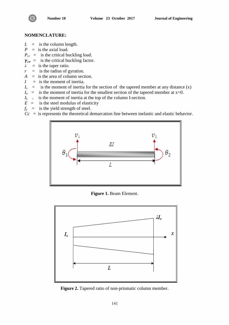
Journal of Engineering Volume 23 October 2017 Number 10
414
NOMENCLATURE:
L = is the column length.
P = is the axial load.
Pcr = is the critical buckling load.
= is the critical buckling factor.
λ = is the taper ratio.
r = is the radius of gyration.
A = is the area of column section.
I = is the moment of inertia.
Ix = is the moment of inertia for the section of the tapered member at any distance (x)
Io = is the moment of inertia for the smallest section of the tapered member at x=0.
IL = is the moment of inertia at the top of the column I-section.
E = is the steel modulus of elasticity
fy = is the yield strength of steel.
Cc = is represents the theoretical demarcation line between inelastic and elastic behavior.
Figure 1. Beam Element.
Figure 2. Tapered ratio of non-prismatic column member.
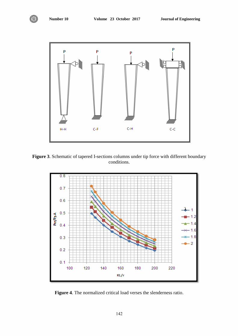
Journal of Engineering Volume 23 October 2017 Number 10
411
Figure 3. Schematic of tapered I-sections columns under tip force with different boundary
conditions.
Figure 4. The normalized critical load verses the slenderness ratio.
λ
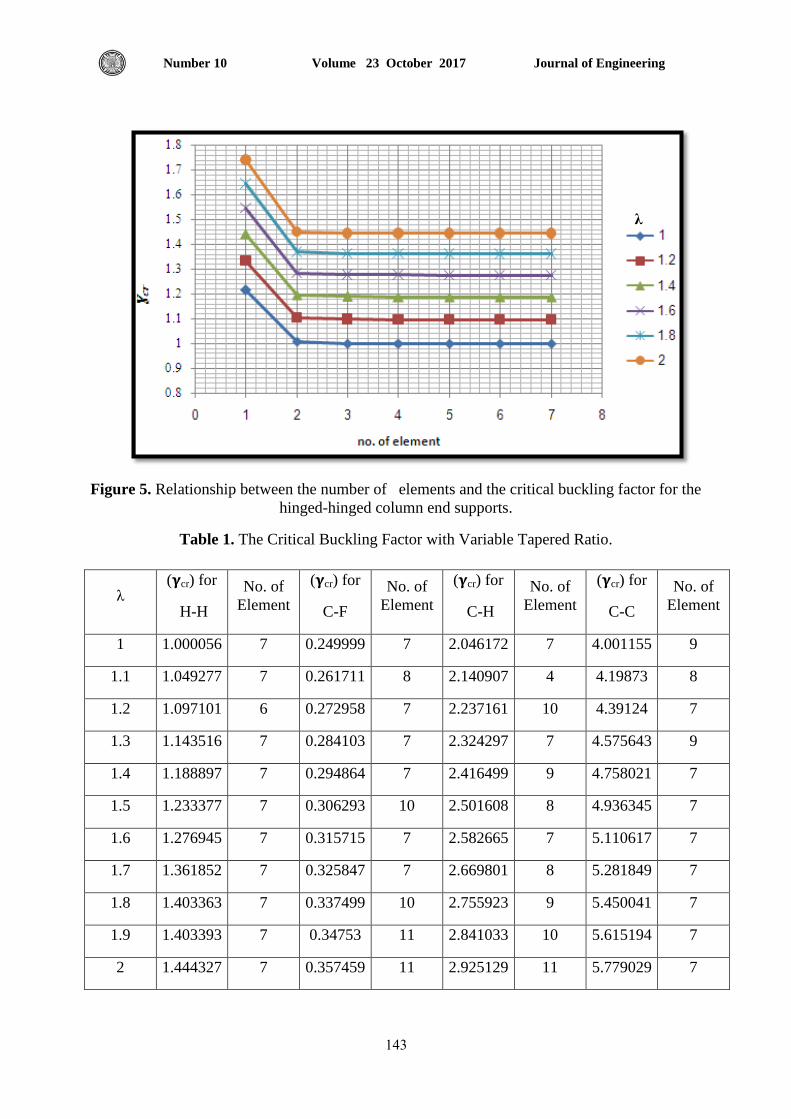
Journal of Engineering Volume 23 October 2017 Number 10
413
Figure 5. Relationship between the number of elements and the critical buckling factor for the
hinged-hinged column end supports.
Table 1. The Critical Buckling Factor with Variable Tapered Ratio.
λ ( cr) for
H-H
No. of
Element
( cr) for
C-F
No. of
Element
( cr) for
C-H
No. of
Element
( cr) for
C-C
No. of
Element
1 1.000056 7 0.249999 7 2.046172 7 4.001155 9
1.1 1.049277 7 0.261711 8 2.140907 4 4.19873 8
1.2 1.097101 6 0.272958 7 2.237161 10 4.39124 7
1.3 1.143516 7 0.284103 7 2.324297 7 4.575643 9
1.4 1.188897 7 0.294864 7 2.416499 9 4.758021 7
1.5 1.233377 7 0.306293 10 2.501608 8 4.936345 7
1.6 1.276945 7 0.315715 7 2.582665 7 5.110617 7
1.7 1.361852 7 0.325847 7 2.669801 8 5.281849 7
1.8 1.403363 7 0.337499 10 2.755923 9 5.450041 7
1.9 1.403393 7 0.34753 11 2.841033 10 5.615194 7
2 1.444327 7 0.357459 11 2.925129 11 5.779029 7
λ
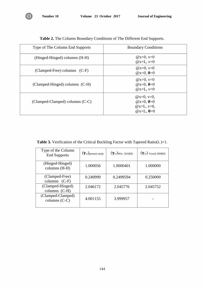
Journal of Engineering Volume 23 October 2017 Number 10
411
Table 2. The Column Boundary Conditions of The Different End Supports.
Type of The Column End Supports Boundary Conditions
(Hinged-Hinged) columns (H-H) @x=0, v=0
@x=L, v=0
(Clamped-Free) columns (C-F) @x=0, v=0
@x=0, =0
(Clamped-Hinged) columns (C-H)
@x=0, v=0
@x=0, =0
@x=L, v=0
(Clamped-Clamped) columns (C-C)
@x=0, v=0,
@x=0, =0
@x=L, v=0,
@x=L, =0
Table 3. Verification of the Critical Buckling Factor with Tapered Ratio(λ )=1.
Type of the Column
End Supports ( cr)present study ( cr)Wie. 2010[8] ( cr) Yossif.2008[9]
(Hinged-Hinged)
columns (H-H) 1.000056 1.0000401 1.000000
(Clamped-Free)
columns (C-F) 0.249999 0.2499594 0.250000
(Clamped-Hinged)
columns (C-H) 2.046172 2.045776 2.045752
(Clamped-Clamped)
columns (C-C)
4.001155 3.999957 -
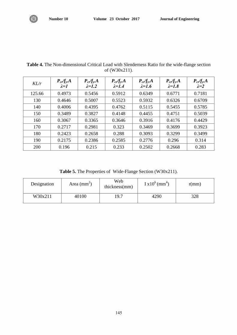
Journal of Engineering Volume 23 October 2017 Number 10
411
Table 4. The Non-dimensional Critical Load with Slenderness Ratio for the wide-flange section
of (W30x211).
KL/r Pcr/fy.A
λ=1
Pcr/fy.A
λ=1.2
Pcr/fy.A
λ=1.4
Pcr/fy.A
λ=1.6
Pcr/fy.A
λ=1.8
Pcr/fy.A
λ=2
125.66 0.4973 0.5456 0.5912 0.6349 0.6771 0.7181
130 0.4646 0.5007 0.5523 0.5932 0.6326 0.6709
140 0.4006 0.4395 0.4762 0.5115 0.5455 0.5785
150 0.3489 0.3827 0.4148 0.4455 0.4751 0.5039
160 0.3067 0.3365 0.3646 0.3916 0.4176 0.4429
170 0.2717 0.2981 0.323 0.3469 0.3699 0.3923
180 0.2423 0.2658 0.288 0.3093 0.3299 0.3499
190 0.2175 0.2386 0.2585 0.2776 0.296 0.314
200 0.196 0.215 0.233 0.2502 0.2668 0.283
Table 5. The Properties of Wide-Flange Section (W30x211).
Designation Area (mm2)
Web
thickness(mm) I x10
6 (mm
4) r(mm)
W30x211 40100 19.7 4290 328
Journal of Engineering Volume 23 October 2017
Number 10
646
Study the Effects of Microwave Furnace Heat on The
Mechanical Properties and Estimated Fatigue life of AA2024-T3
Dr. Ahmed Adnan AL-Qaisy
Lecturer
Mechanical Engineering Department
University of Technology
Sameh Fareed Hasan Najmuldeen Yousif Mahmood
Engineer Assistant Lecturer
Ministry of Science and Technology Mechanical Engineering Department
Industrial Development & Research Director University of Technology
ABSTRACT
This research aims to study the effect of microwave furnace heat on the mechanical properties
and fatigue life of aluminum alloy (AA 2024-T3). Four conditions were used inside microwave
furnace (specimens subjected to heat as dry for 30 and 60min. and specimens subjected to heat as
wet (water) for 30 and 60 min.), and compared all results with original alloy (AA 2024-T3).
Tensile, fatigue, hardness and surface roughness tests were used in this investigation. It is found
that hardness of dry conditions is higher than wet conditions and it increases with increasing of
time duration inside microwave furnace for dry and wet conditions. Also, tensile strength has the
same behavior of hardness, but it increases with decreasing of time. Dry condition for 60 min.
shows the higher fatigue strength than other conditions. Surface roughness parameter (Ra) of dry
conditions is higher than wet conditions and it decreases with increasing of duration of time.
Key words: Microwave Furnace, Mechanical Properties, Fatigue Life.
على الخىاص الويكايكيت الوايكروويف أفراىاجوت عي الحرارة الدراست تأثير
T3-2024وعور الكالل لسبيكت األلىهيىم
الجبار أحوذ عذاى عبذد. هذرس
قسى انهذست انيكايكيت
انجايعت انتكىنىجيت
جن الذيي يىسف هحوىد ساهح فريذ حسي
هذرس هساعذ هذس ه
قسى انهذست انيكايكيت وسارة انعهىو وانتكىنىجيا
انجايعت انتكىنىجيت دائزة انبحث وانتطىيز انظاعي
الخالصتنذراست تأثيز حزارة افزا انايكزويف عهى انخىاص انيكايكيت وعز انكالل نسبيكت االنيىو يهذف هذا انبحث
(AA2024-T3 63دقيقت و 03(. تى استخذاو ابزع حاالث داخم افزا انايكزويف )عياث جافت تتعزع انى حزارة نذة
قيقت(. في هذا انبحث تى استخذاو اختبار انشذ , انكالل , د 63دقيقت و 03دقيقت و عياث رطبت )اناء( تتعزع انى حزارة نذة
انظالدة و خشىت انسطح. وجذث ا االطالدة نهحاالث انجافت اعهى ي انحاالث انزطبت وتتاقض انظالدة بشيادة انشي داخم
تشداد يقاويت انشذ بقظا فز انايكزويف بانسبت نهحاالث انجافت وانزطبت. يقاويت انشذ نها فس سهىك انظالدة ايضا ونك
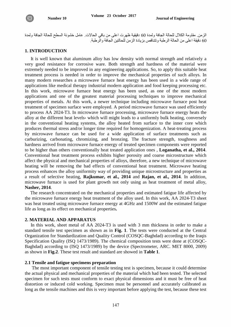
Journal of Engineering Volume 23 October 2017
Number 10
647
دقيقيت ظهزث اعهى ي باقي انحاالث. عايم خشىت انسطح نهحانت انجافت ونذة 63انشي. يقاويت انكالل نهحانت انجافت ونذة
دقيقت اعهى ي انحانت انزطبت وتتاقض بشيادة انشي نهحانتي انجافت وانزطبت. 63
1. INTRODUCTION
It is well known that aluminum alloy has low density with normal strength and relatively a
very good resistance for corrosive ware. Both strength and hardness of the material were
extremely needed to be improved in any engineering applications. So, to apply this suitable heat
treatment process is needed in order to improve the mechanical properties of such alloys. In
many modern researches a microwave furnace heat energy has been used in a wide range of
applications like medical therapy industrial modern application and food keeping processing etc.
In this work, microwave furnace heat energy has been used, as one of the most modern
applications and one of the greatest material processing techniques to improve mechanical
properties of metals. At this work, a newer technique including microwave furnace post heat
treatment of specimen surface were employed. A period microwave furnace was used efficiently
to process AA 2024-T3. In microwave furnace processing, microwave furnace energy heats the
alloy at the different heat levels, which will might leads to a uniformly bulk heating, conversely
in the conventional heating systems, the alloy heated from surface to the inner core which
produces thermal stress and/or longer time required for homogenization. A heat-treating process
by microwave furnace can be used for a wide application of surface treatments such as
carburizing, carbonating, chromizing, and bronzing. The fracture strength, toughness and
hardness arrived from microwave furnace energy of treated specimen components were reported
to be higher than others conventionally heat treated application ones , Loganatha, et al., 2014.
Conventional heat treatment process exhibits higher porosity and coarse microstructure which
affect the physical and mechanical properties of alloys, therefore, a new technique of microwave
heating will be removing the bad effects of conventional heat treatment. Microwave heating
process enhances the alloy uniformity way of providing unique microstructure and properties as
a result of selective heating, Rajkumar, et al., 2014 and Rajan, et al., 2014. In addition,
microwave furnace is used for plant growth not only using as heat treatment of metal alloy,
Nasher, 2014.
The research concentrated on the mechanical properties and estimated fatigue life affected by
the microwave furnace energy heat treatment of the alloy used. In this work, AA 2024-T3 sheet
was heat treated using microwave furnace energy at 4GHz and 1500W and the estimated fatigue
life as long as its effect on mechanical properties.
2. MATERIAL AND APPARATUS
In this work, sheet metal of AA 2024-T3 is used with 3 mm thickness in order to make a
standard tensile test specimen as shown as in Fig. 1. The tests were conducted at the Central
Organization for Standardization and Quality Control (COSQC-Baghdad) according to the Iraqis
Specification Quality (ISQ 1473/1989). The chemical composition tests were done at (COSQC-
Baghdad) according to (ISQ 1473/1989) by the device (Spectrometer, ARC. MET 8000, 2009)
as shown in Fig.2. These test result and standard are showed in Table 1.
2.1 Tensile and fatigue specimens preparation
The most important component of tensile testing test is specimen, because it could determine
the actual physical and mechanical properties of the material which had been tested. The selected
specimen for such tests must conform to exact physical dimensions and it must be free of heat
distortion or induced cold working. Specimen must be personnel and accurately calibrated as
long as the tensile machines and this is very important before applying the test, because these test

Journal of Engineering Volume 23 October 2017
Number 10
648
results were based on the accuracy and quality of the test specimen that been used. Tinius Olsen
tensile machine is used in this investigation as showing in Fig. 3. A preparation steps including a
precision milling machine, highly skilled machinist and considerably highly skills hand finishing
can achieve the required configurations of the test specimen needed, ASTM, 2012.
To achieve accurate results, a test specimen must be prepared accurately and properly. The
following rules are suggested for general guidance:
a. Using Standard dimensions and sizes such as ASTM standards and like.
b. Surface finishing is very important in preparing tensile test specimens because it might be
affecting on the results.
Other preparation concludes:
1. Grinding the specimen faces and sides with grinding papers (Silicon Carbide) starting from
120, 320, 500, 1000 and 2000 type .
2. Polishing the specimen by polishing instrument (Alumina Powder) of a grain size 0.5 µm.
3. Washing the specimen by water, oil soap and alcohol to remove grinding and polishing
remained particles.
4. Finally, smoothly clean the specimen by soft silky fabric until you should almost see
yourself on it. Fig. 4 shows the specimen before and after polishing.
2.2 Fatigue Test Machine [Avery Standard Test]
In this research, a fully reversed reciprocating plane bending fatigue testing machine (Bend
Test) type Avery Model 7305 with stress ratio R = -1 was used, see Fig. 5. To perform the
tests, the following steps should be followed:
Step 1: Preparing the Machine:
As said, the machine should be calibrated to stress ratio R = -1 and for that two dial gages
were used as shown in Fig. 5.
Step 2: Machine Calibration:
Static Calibration: In machines, it is importance to know exactly the speed of the machine,
as an error in its speed corresponds might be to a doubled error in the applied load where the
load is produced by centrifugal forces or by reciprocating masses. Therefore, the motor speed
must be checked and calibrated with the standard. Table 2 is illustrated the instruction manual
of the machine.
Dynamic Calibration: During the operation of the testing machine, a new source of error
sometimes appears; these errors come from the arrived vibration of rotating parts of the
machine, which might lead to errors in the estimated results of the test. In the present work, a
rubber isolator was used between the machine and the grand table to eliminate the inertia
effects, ASME, 2009.
2.3 Other Mechanical Properties Tests
Other tests included hardness test according to refrence, ASTM E 110 – 82, 2002, and
surface roughness test according to Mitutoyo Standard Test. The first test was done by
(Rockwell Hardness Testing Machine, the values are converted from Bernill Hardness value) as
showing in Fig. 6, while the second test was done by Mitutoyo Surface Roughness Testing
Machine as illustrated in Fig. 7, all tests were made by the COSQC-Baghdad according to the
(ISQ 1475~1476/1989).
2.4 Experimental Work
Microwave furnace type Daewoo is used to achieve a heat treatment for all specimens as
showing in Fig. 8. Figs. 9 and 10 are showing tensile and fatigue specimens. There are 12th
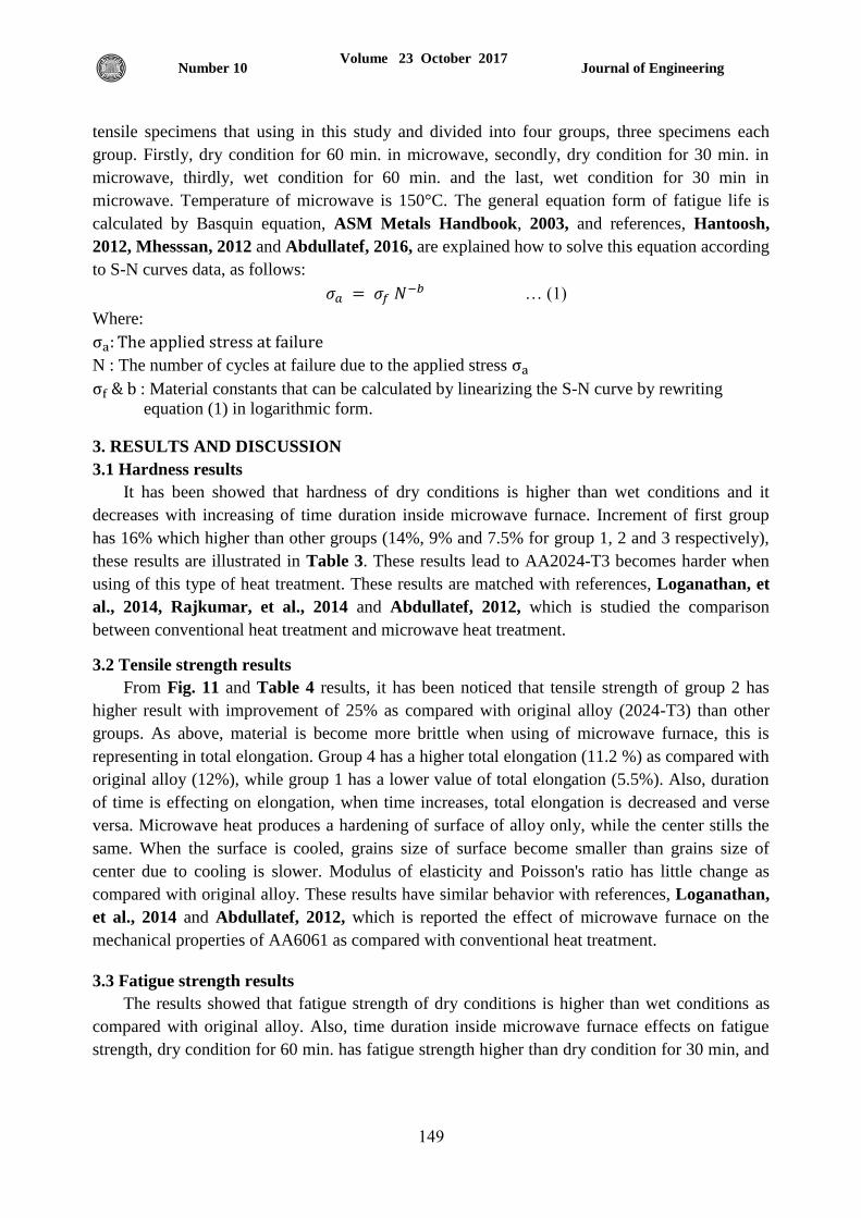
Journal of Engineering Volume 23 October 2017
Number 10
649
tensile specimens that using in this study and divided into four groups, three specimens each
group. Firstly, dry condition for 60 min. in microwave, secondly, dry condition for 30 min. in
microwave, thirdly, wet condition for 60 min. and the last, wet condition for 30 min in
microwave. Temperature of microwave is 150°C. The general equation form of fatigue life is
calculated by Basquin equation, ASM Metals Handbook, 2003, and references, Hantoosh,
2012, Mhesssan, 2012 and Abdullatef, 2016, are explained how to solve this equation according
to S-N curves data, as follows:
… (1)
Where:
N : The number of cycles at failure due to the applied stress
: Material constants that can be calculated by linearizing the S-N curve by rewriting
equation (1) in logarithmic form.
3. RESULTS AND DISCUSSION
3.1 Hardness results
It has been showed that hardness of dry conditions is higher than wet conditions and it
decreases with increasing of time duration inside microwave furnace. Increment of first group
has 16% which higher than other groups (14%, 9% and 7.5% for group 1, 2 and 3 respectively),
these results are illustrated in Table 3. These results lead to AA2024-T3 becomes harder when
using of this type of heat treatment. These results are matched with references, Loganathan, et
al., 2014, Rajkumar, et al., 2014 and Abdullatef, 2012, which is studied the comparison
between conventional heat treatment and microwave heat treatment.
3.2 Tensile strength results
From Fig. 11 and Table 4 results, it has been noticed that tensile strength of group 2 has
higher result with improvement of 25% as compared with original alloy (2024-T3) than other
groups. As above, material is become more brittle when using of microwave furnace, this is
representing in total elongation. Group 4 has a higher total elongation (11.2 %) as compared with
original alloy (12%), while group 1 has a lower value of total elongation (5.5%). Also, duration
of time is effecting on elongation, when time increases, total elongation is decreased and verse
versa. Microwave heat produces a hardening of surface of alloy only, while the center stills the
same. When the surface is cooled, grains size of surface become smaller than grains size of
center due to cooling is slower. Modulus of elasticity and Poisson's ratio has little change as
compared with original alloy. These results have similar behavior with references, Loganathan,
et al., 2014 and Abdullatef, 2012, which is reported the effect of microwave furnace on the
mechanical properties of AA6061 as compared with conventional heat treatment.
3.3 Fatigue strength results
The results showed that fatigue strength of dry conditions is higher than wet conditions as
compared with original alloy. Also, time duration inside microwave furnace effects on fatigue
strength, dry condition for 60 min. has fatigue strength higher than dry condition for 30 min, and
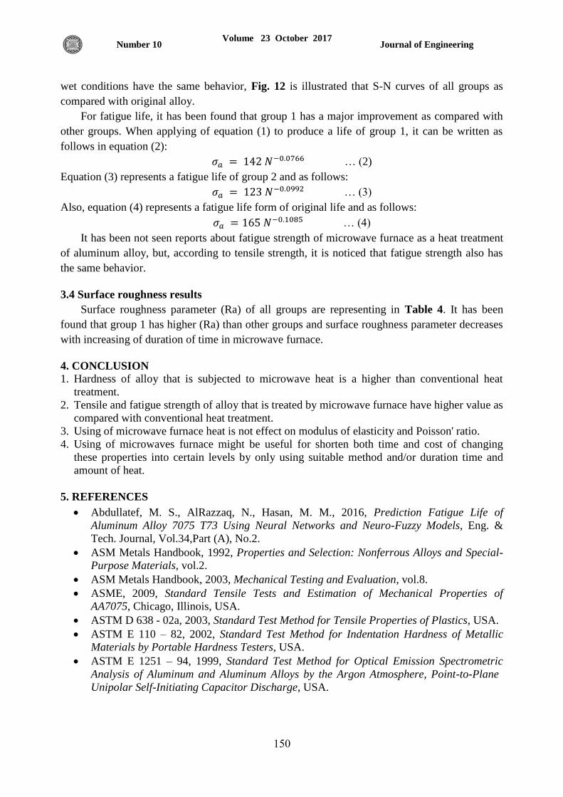
Journal of Engineering Volume 23 October 2017
Number 10
653
wet conditions have the same behavior, Fig. 12 is illustrated that S-N curves of all groups as
compared with original alloy.
For fatigue life, it has been found that group 1 has a major improvement as compared with
other groups. When applying of equation (1) to produce a life of group 1, it can be written as
follows in equation (2):
… (2)
Equation (3) represents a fatigue life of group 2 and as follows:
… (3)
Also, equation (4) represents a fatigue life form of original life and as follows:
… (4)
It has been not seen reports about fatigue strength of microwave furnace as a heat treatment
of aluminum alloy, but, according to tensile strength, it is noticed that fatigue strength also has
the same behavior.
3.4 Surface roughness results
Surface roughness parameter (Ra) of all groups are representing in Table 4. It has been
found that group 1 has higher (Ra) than other groups and surface roughness parameter decreases
with increasing of duration of time in microwave furnace.
4. CONCLUSION
1. Hardness of alloy that is subjected to microwave heat is a higher than conventional heat
treatment.
2. Tensile and fatigue strength of alloy that is treated by microwave furnace have higher value as
compared with conventional heat treatment.
3. Using of microwave furnace heat is not effect on modulus of elasticity and Poisson' ratio.
4. Using of microwaves furnace might be useful for shorten both time and cost of changing
these properties into certain levels by only using suitable method and/or duration time and
amount of heat.
5. REFERENCES
Abdullatef, M. S., AlRazzaq, N., Hasan, M. M., 2016, Prediction Fatigue Life of
Aluminum Alloy 7075 T73 Using Neural Networks and Neuro-Fuzzy Models, Eng. &
Tech. Journal, Vol.34,Part (A), No.2.
ASM Metals Handbook, 1992, Properties and Selection: Nonferrous Alloys and Special-
Purpose Materials, vol.2.
ASM Metals Handbook, 2003, Mechanical Testing and Evaluation, vol.8.
ASME, 2009, Standard Tensile Tests and Estimation of Mechanical Properties of
AA7075, Chicago, Illinois, USA.
ASTM D 638 - 02a, 2003, Standard Test Method for Tensile Properties of Plastics, USA.
ASTM E 110 – 82, 2002, Standard Test Method for Indentation Hardness of Metallic
Materials by Portable Hardness Testers, USA.
ASTM E 1251 – 94, 1999, Standard Test Method for Optical Emission Spectrometric
Analysis of Aluminum and Aluminum Alloys by the Argon Atmosphere, Point-to-Plane Unipolar Self-Initiating Capacitor Discharge, USA.
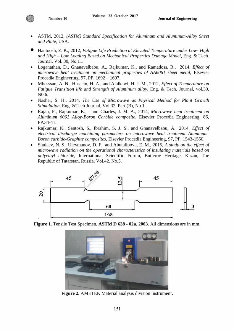
Journal of Engineering Volume 23 October 2017
Number 10
656
ASTM, 2012, (ASTM) Standard Specification for Aluminum and Aluminum-Alloy Sheet
and Plate, USA.
Hantoosh, Z. K., 2012, Fatigue Life Prediction at Elevated Temperature under Low- High
and High – Low Loading Based on Mechanical Properties Damage Model, Eng. & Tech.
Journal, Vol. 30, No.11. Loganathan, D., Gnanavelbabu, A., Rajkumar, K., and Ramadoss, R., 2014, Effect of
microwave heat treatment on mechanical properties of AA6061 sheet metal, Elsevier
Procedia Engineering, 97, PP. 1692 – 1697.
Mhesssan, A. N., Hussein, H. A., and Alalkawi, H. J. M., 2012, Effect of Temperature on
Fatigue Transition life and Strength of Aluminum alloy, Eng. & Tech. Journal, vol.30,
N0.6.
Nasher, S. H., 2014, The Use of Microwave as Physical Method for Plant Growth
Stimulation, Eng. &Tech.Journal, Vol.32, Part (B), No.1.
Rajan, P., Rajkumar, K., , and Charles, J. M. A., 2014, Microwave heat treatment on
Aluminum 6061 Alloy-Boron Carbide composite, Elsevier Procedia Engineering, 86,
PP.34-41.
Rajkumar, K., Santosh, S., Ibrahim, S. J. S., and Gnanavelbabu, A., 2014, Effect of
electrical discharge machining parameters on microwave heat treatment Aluminum-
Boron carbide-Graphite composites, Elsevier Procedia Engineering, 97, PP. 1543-1550.
Shulaev, N. S., Uleymanov, D. F., and Abutalipova, E. M., 2015, A study on the effect of
microwave radiation on the operational characteristics of insulating materials based on
polyvinyl chloride, International Scientific Forum, Butlerov Heritage, Kazan, The
Republic of Tatarstan, Russia, Vol.42. No.5.
Figure 1. Tensile Test Specimen, ASTM D 638 - 02a, 2003. All dimensions are in mm.
Figure 2. AMETEK Material analysis division instrument.
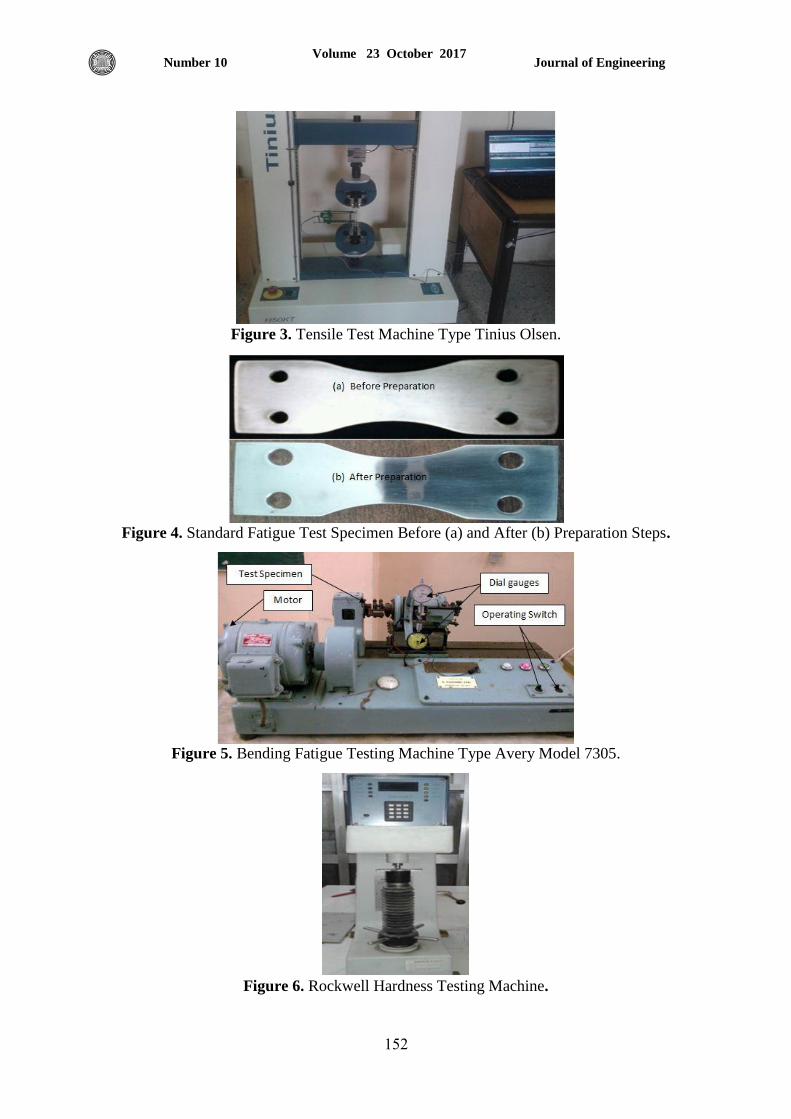
Journal of Engineering Volume 23 October 2017
Number 10
651
Figure 3. Tensile Test Machine Type Tinius Olsen.
Figure 4. Standard Fatigue Test Specimen Before (a) and After (b) Preparation Steps.
Figure 5. Bending Fatigue Testing Machine Type Avery Model 7305.
Figure 6. Rockwell Hardness Testing Machine.
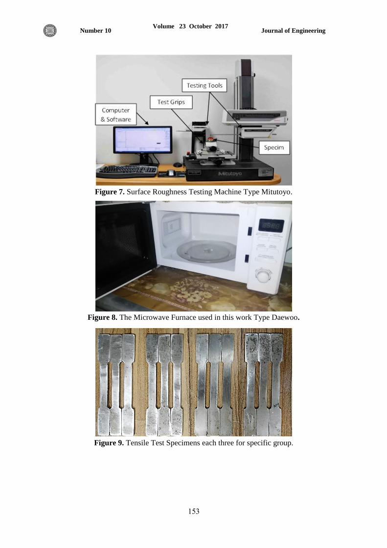
Journal of Engineering Volume 23 October 2017
Number 10
650
Figure 7. Surface Roughness Testing Machine Type Mitutoyo.
Figure 8. The Microwave Furnace used in this work Type Daewoo.
Figure 9. Tensile Test Specimens each three for specific group.
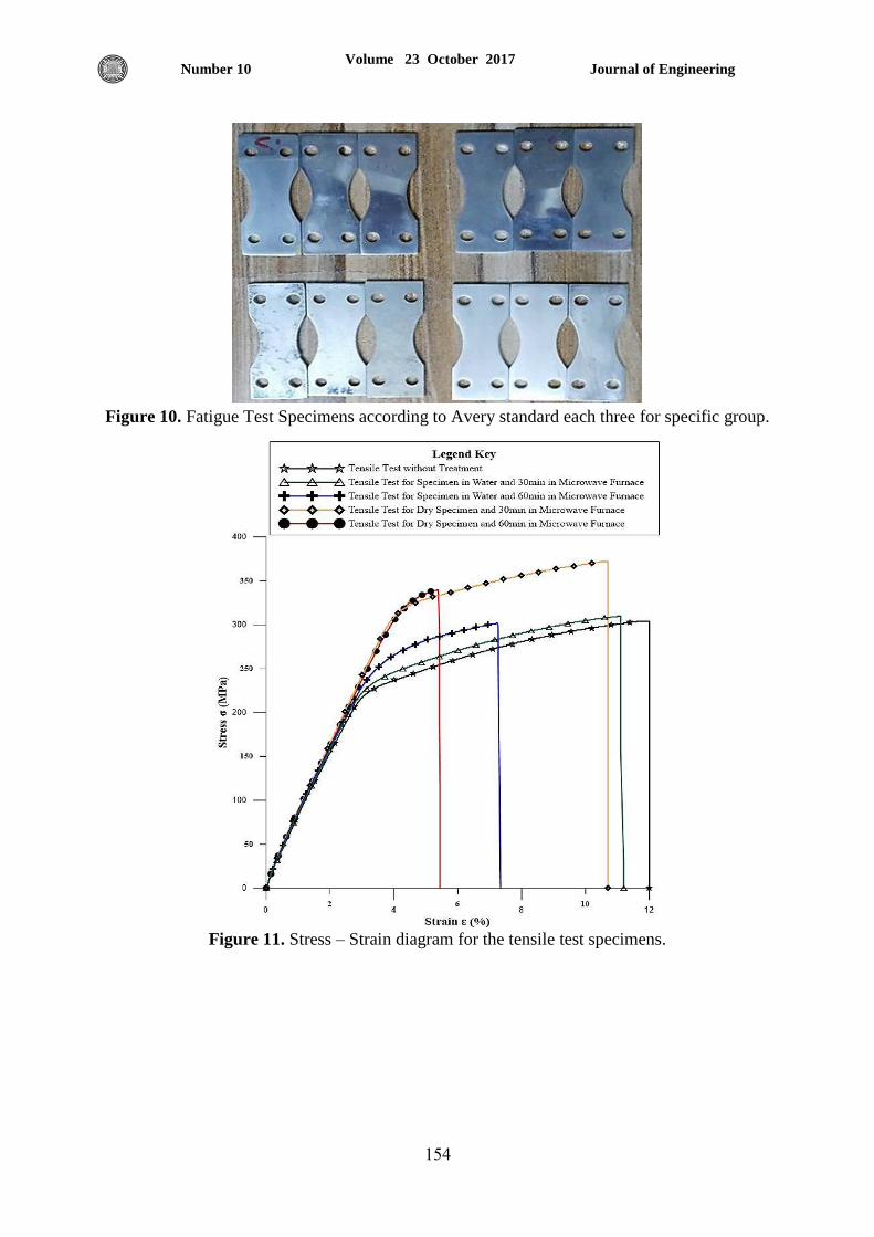
Journal of Engineering Volume 23 October 2017
Number 10
654
Figure 10. Fatigue Test Specimens according to Avery standard each three for specific group.
Figure 11. Stress – Strain diagram for the tensile test specimens.
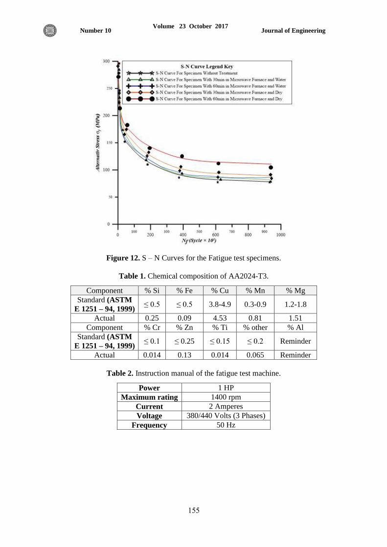
Journal of Engineering Volume 23 October 2017
Number 10
655
Figure 12. S – N Curves for the Fatigue test specimens.
Table 1. Chemical composition of AA2024-T3.
Component % Si % Fe % Cu % Mn % Mg
Standard (ASTM
E 1251 – 94, 1999) ≤ 0.5 ≤ 0.5 3.8-4.9 0.3-0.9 1.2-1.8
Actual 0.25 0.09 4.53 0.81 1.51
Component % Cr % Zn % Ti % other % Al
Standard (ASTM
E 1251 – 94, 1999) ≤ 0.1 ≤ 0.25 ≤ 0.15 ≤ 0.2 Reminder
Actual 0.014 0.13 0.014 0.065 Reminder
Table 2. Instruction manual of the fatigue test machine.
Power 1 HP
Maximum rating 1400 rpm
Current 2 Amperes
Voltage 380/440 Volts (3 Phases)
Frequency 50 Hz
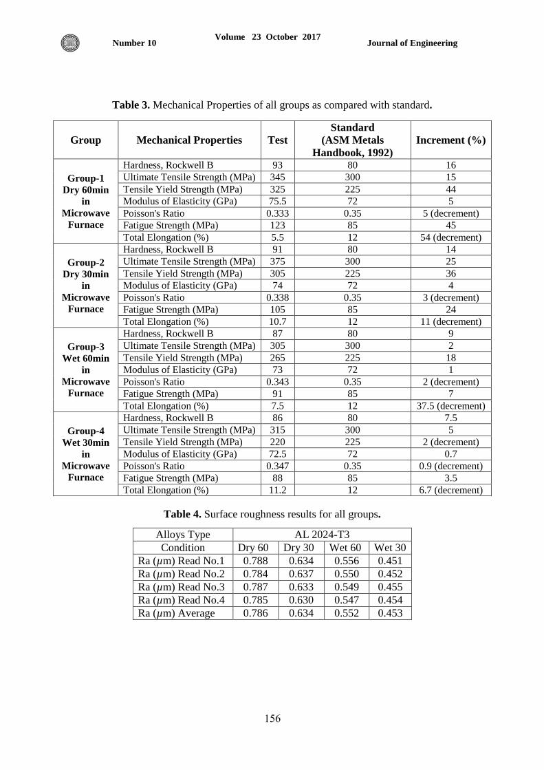
Journal of Engineering Volume 23 October 2017
Number 10
656
Table 3. Mechanical Properties of all groups as compared with standard.
Table 4. Surface roughness results for all groups.
Alloys Type AL 2024-T3
Condition Dry 60 Dry 30 Wet 60 Wet 30
Ra (µm) Read No.1 0.788 0.634 0.556 0.451
Ra (µm) Read No.2 0.784 0.637 0.550 0.452
Ra (µm) Read No.3 0.787 0.633 0.549 0.455
Ra (µm) Read No.4 0.785 0.630 0.547 0.454
Ra (µm) Average 0.786 0.634 0.552 0.453
Group Mechanical Properties Test
Standard
(ASM Metals
Handbook, 1992)
Increment (%)
Group-1
Dry 60min
in
Microwave
Furnace
Hardness, Rockwell B 93 80 16
Ultimate Tensile Strength (MPa) 345 300 15
Tensile Yield Strength (MPa) 325 225 44
Modulus of Elasticity (GPa) 75.5 72 5
Poisson's Ratio 0.333 0.35 5 (decrement)
Fatigue Strength (MPa) 123 85 45
Total Elongation (%) 5.5 12 54 (decrement)
Group-2
Dry 30min
in
Microwave
Furnace
Hardness, Rockwell B 91 80 14
Ultimate Tensile Strength (MPa) 375 300 25
Tensile Yield Strength (MPa) 305 225 36
Modulus of Elasticity (GPa) 74 72 4
Poisson's Ratio 0.338 0.35 3 (decrement)
Fatigue Strength (MPa) 105 85 24
Total Elongation (%) 10.7 12 11 (decrement)
Group-3
Wet 60min
in
Microwave
Furnace
Hardness, Rockwell B 87 80 9
Ultimate Tensile Strength (MPa) 305 300 2
Tensile Yield Strength (MPa) 265 225 18
Modulus of Elasticity (GPa) 73 72 1
Poisson's Ratio 0.343 0.35 2 (decrement)
Fatigue Strength (MPa) 91 85 7
Total Elongation (%) 7.5 12 37.5 (decrement)
Group-4
Wet 30min
in
Microwave
Furnace
Hardness, Rockwell B 86 80 7.5
Ultimate Tensile Strength (MPa) 315 300 5
Tensile Yield Strength (MPa) 220 225 2 (decrement)
Modulus of Elasticity (GPa) 72.5 72 0.7
Poisson's Ratio 0.347 0.35 0.9 (decrement)
Fatigue Strength (MPa) 88 85 3.5
Total Elongation (%) 11.2 12 6.7 (decrement)

October
2017
Number 10
Volume 23
E-ISSN 2520-3339
P-ISSN 1726-4073
10 العدد23 المجلد
تشرين االول2017
E-ISSN 2520-3339
P-ISSN 1726-4073

رقم االيداع في دار الكتب والوثائق ببغداد
3122لسنة 3342