Embed Size (px)
Citation preview

University of Calgary
PRISM: University of Calgary's Digital Repository
Graduate Studies The Vault: Electronic Theses and Dissertations
2013-09-09
Experimental Evaluation of the Effect of Carbonate
Heterogeneity on Oil Recovery to Water and Gas
Injections
Alharbi, Ahmad
Alharbi, A. (2013). Experimental Evaluation of the Effect of Carbonate Heterogeneity on Oil
Recovery to Water and Gas Injections (Unpublished doctoral thesis). University of Calgary,
Calgary, AB. doi:10.11575/PRISM/26058
http://hdl.handle.net/11023/933
doctoral thesis
University of Calgary graduate students retain copyright ownership and moral rights for their
thesis. You may use this material in any way that is permitted by the Copyright Act or through
licensing that has been assigned to the document. For uses that are not allowable under
copyright legislation or licensing, you are required to seek permission.
Downloaded from PRISM: https://prism.ucalgary.ca

UNIVERSITY OF CALGARY
Experimental Evaluation of the Effect of Carbonate Heterogeneity on Oil Recovery to Water and
Gas Injections
by
Ahmad Mubarak Alharbi
A THESIS
SUBMITTED TO THE FACULTY OF GRADUATE STUDIES
IN PARTIAL FULFILMENT OF THE REQUIREMENTS FOR THE
DEGREE OF DOCTOR OF PHILOSOPHY
DEPARTMENT OF CHEMICAL AND PETROLEUM ENGINEERING
CALGARY, ALBERTA
SEPTEMBER, 2013
© Ahmad Mubarak Alharbi 2013

ii
Abstract
The natural structural variations in petroleum carbonate reservoirs often dictate the best
displacement strategy and always impact the ultimate recovery. Quantifying the impact of these
structural heterogeneities can ultimately guide reservoir performance optimization techniques
such as well placement and can reduce the uncertainty in reserve calculations. Nuclear Magnetic
Resonance (NMR) and Computerized Tomography (CT) were used to build on previous work
and add mechanistic information that in the past has been unattainable.
This study investigates the effect of moderate carbonate heterogeneity on oil recovery from
immiscible N2 gas injection. Initially, the variations of porosity and permeability within the scale
of a core plug sample using NMR and CT are charactrized. The results from visually classifying
51 core samples showed that the samples can be classified into three main heterogeneity groups:
low rock heterogeneity (LRH), moderate rock heterogeneity (MRH), and high rock heterogeneity
(HRH). Additional rock characterization was conducted including wettability, mercury injection,
and petrographic image analysis. The results indicated intermediate wetting system, various pore
size distributions, and complex diagenetic process, respectively.
A new permeability-predictor correlation was established, by linking the Kozeny-Carman (K-C)
empirical correlation with the NMR total surface area of pores, and it was verified using the
selected samples. The results showed a good match between the measured and predicted
permeabilities, suggesting that the pore connectivity in these specific rocks may not be critical to
capillary based recovery processes.
Based on the rock heterogeneity classification results, centrifuge and gasflood experiments were
carried out. The centrifuge experiments, performed at 80oC, were conducted on nine core
samples. The gasflood experiments were performed on nine core stacks, in which six runs were

iii
conducted at 80oC and a pore-pressure of 1034 kPa while three runs were performed at 80
oC and
a pore-pressure of 17237 kPa. Five of the low pore-pressure’s (LPP) experiments were
conducted in secondary recovery mode while one run was performed in tertiary recovery mode.
Three of the high pore-pressure’s (HPP) gasfloods were conducted in secondary recovery mode.
All of the gas-oil displacement experiments were carried out to evaluate the effect of single-and
multi-rock heterogeneities on oil recovery.
The results from the centrifuge experiments suggested that oil recovery is generally less sensitive
to rock heterogeneity under favourable gravity drainage conditions. On the other hand, oil
recovery from the LPP gasfloods showed a monotonic trend with rock heterogeneity. The LRH
rocks showed the highest oil recovery (41.94% OOIP) while the HRH rocks showed the lowest
oil recovery (29.33% OOIP). The oil recovery from the multi-rock heterogeneity showed
outstanding results (47.82% OOIP) as compared to the LRH, MRH, and HRH results (41.94%,
34.02%, and 29.33% of OOIP, respectively). The results from the high pore-pressure’s (HPP)
runs showed almost similar oil recovery trend with rock heterogeneity to that from the LPP
gasfloods.
The injection of water as a secondary recovery process resulted in higher oil recovery (64.78%
OOIP) than all secondary gasfloods. Injecting N2 gas in tertiary mode resulted in similar
recovery to the MIRH secondary mode (34.80% ROIP vs. 34.02% OOIP). However, if the
waterflood recovery (prior to N2) is considered, the ultimate recovery of the tertiary mode is
much higher at a later time. The combined recovery from waterflood and gasflood (tertiary) is
found to be 83.23% of OOIP. These results suggest that implementing secondary waterflooding
and tertiary gas injection in the actual reservoir could be very beneficial.

iv
A lab simulator was used to history match the results from secondary gasfloods in order to
estimate the “true” oil recovery. It was found that the HRH rocks were highly affected by
capillary end-effect as compared to the MRH rocks. The corrected oil recovery for the HRH
rocks was higher than the MRH rocks leading to the conclusion that the HRH may not be
harmful rock heterogeneity to the capillary number based recovery process.

v
Acknowledgements
I would like to thank Dr. A. Kantzas for his supervision and support during this work.
I am heartily thankful to Dr. S. Kryuchkov and Dr. J. Bryan whose office doors have been
always open for my questions. I really appreciate their invaluable advice and consultations.
I also would like to thank my committee members Dr. B. Maini and Dr. R. Aguilera for serving
on my committee and for their support and interest in my research.
Thanks also go to my friends and colleagues and the department faculty and staff for making my
time at the University of Calgary a great experience. Special thanks to M. Benedek, M. Erath, J.
Dong, and I. Tanski from TIPM, for their support with my experimental work.
Thanks to my siblings for their encouragement, motivation, and sincere prayers. Finally, I want
to extend my gratitude to Saudi Aramco for sponsoring my PhD studies at the University of
Calgary.

vi
Dedication
I wish to dedicate this dissertation to:
My mother, to whom I owe everything in my life, may Allah have mercy on her soul and
grant her Jannat Alfirdous;
My father, for believing in me, may Allah give him Barakah and good health in his life;
Special dedication is due to:
My wife, Nouf Alharbi, for the love and support she has given me throughout my studies
at the University of Calgary.
Finally,
To my wonderful sons, Malik and Muhammad,
and my lovely daughters, Manar and Misk.

vii
Table of Contents
Abstract ............................................................................................................................... ii Acknowledgements ..............................................................................................................v
Dedication .......................................................................................................................... vi Table of Contents .............................................................................................................. vii List of Tables .......................................................................................................................x List of Figures and Illustrations ........................................................................................ xii List of Symbols, Abbreviations and Nomenclature ......................................................... xvi
CHAPTER ONE: INTRODUCTION ..................................................................................1
CHAPTER TWO: RESEARCH OBJECTIVES ..................................................................5
CHAPTER THREE: LITERATURE REVIEW ..................................................................7 3.1 Depositional Textures and Diagenetic Processes ......................................................7
3.1.1 Carbonate Porosity ............................................................................................8 3.2 How has Heterogeneity been Classified in Carbonate Rocks? ..................................8
3.3 Statistical Characterization of Heterogeneity ..........................................................11 3.3.1 The Dykstra-Parson’s coefficient (VDP) ..........................................................11
3.3.2 The Lorenz Coefficient (LC) ............................................................................12 3.3.3 Coefficient of Variation (Cv) ..........................................................................13
3.4 Effect of Heterogeneity on Residual Oil from Waterflood ......................................13
3.5 Effect of Reservoir Heterogeneity on Oil Recovery from Gas Injection ................17 3.5.1 Effect of Rock Heterogeneity under Miscible Gas Injection ..........................18
3.5.2 Effect of Rock Heterogeneity under Immiscible Gas Injection ......................21 3.5.3 Effect of Wettability ........................................................................................23
3.5.4 Effect of Spreading Coefficient .......................................................................26 3.5.5 Effect of Connate Water Saturation ................................................................28
3.6 The Geological Description of the Reservoir under Study ......................................29
CHAPTER FOUR: RESERVOIR ROCK CHARACTRIZATION ..................................37
4.1 Sample Selection ......................................................................................................37 4.2 Air Permeability and Porosity Measurements .........................................................38 4.3 Mercury Injection and Drainage Capillary Pressure Study .....................................39 4.4 Petrographic Study ...................................................................................................45 4.5 Wettability Characterization Study ..........................................................................49
4.5.1 Wettability Study using the Amott and the USBM Methods ..........................50
4.5.2 Wettability Results ..........................................................................................52
4.6 Characterization of Porosity and Permeability Variation within a Plug Scale ........53 4.6.1 Use of NMR as Permeability Variation Indicator ...........................................53
4.6.1.1 NMR Experimental Work and Data Analysis .......................................56 4.6.2 Use of CT Scanning as a Porosity Variation Indicator ....................................62
4.6.2.1 CT Scanning Experimental Work and Data Analysis ...........................64
4.6.3 Combining NMR and CT Results ...................................................................68 4.6.4 Will this Rock Heterogeneity affects the Capillary Based Production Process?71

viii
CHAPTER FIVE: EXPERIMENTAL APPARATUS AND PROCEDURE ....................77
5.1 EXPEC ARC Coreflood Apparatus .........................................................................77 5.1.1 Injection System ..............................................................................................77 5.1.2 Coreflood Cell .................................................................................................79
5.1.3 Production System ...........................................................................................79 5.1.4 Data Acquisition System .................................................................................79
5.2 In-House Coreflood Apparatus ................................................................................80 5.2.1 Injection System ..............................................................................................80 5.2.2 Coreflood Cell .................................................................................................81
5.2.3 Production System ...........................................................................................81 5.2.4 Data Acquisition System .................................................................................81 5.2.5 The GE CTI X-Ray CT Scanner .....................................................................82
5.3 Testing Procedure ....................................................................................................83
5.3.1 Coreflood Experiments Performed at HPP ......................................................83 5.3.2 Coreflood Experiments Performed at LPP ......................................................85
5.3.3 Centrifuge System ...........................................................................................87 5.4 CT Scan Data Analysis Used in this Study ..............................................................88
CHAPTER SIX: EXPERIMENTAL RESULTS AND DISCUSSIONS ..........................92 6.1 Properties of the Fluids Used in This Study ............................................................92 6.2 Rock Heterogeneity Effect on Oil Recovery from Centrifuge ................................93
6.3 Rock Heterogeneity Effect on Oil Recovery from Corefloods ................................98 6.3.1 Experimental Runs Performed at LPP ...........................................................100
6.3.1.1 Effect of Single Rock Heterogeneity on Oil Recovery ........................101 6.3.2 Experimental Runs Performed at HPP ..........................................................144
CHAPTER SEVEN: HISTORY MATCHING STUDY .................................................152 7.1 Simulator Used in This Study ................................................................................152
7.2 History Matching Experimental Results from Two Phase Flow ...........................152
CHAPTER EIGHT: CONCLUSIONS AND RECOMMENDATIONS .........................162 8.1 Conclusions ............................................................................................................162
8.2 Recommendations ..................................................................................................165
REFERENCES ................................................................................................................167
APPENDIX A: SOME RESULTS FROM MERCURY INJECTION STUDY .............180
APPENDIX B: PETROGRAPHIC STUDY ...................................................................184 B.1. Thin Section Description......................................................................................184 B.2. Thin Section and Samples Photos ........................................................................185
APPENDIX C: CT IMAGES AND CT-POROSITY AND NMR T2 DISTRIBUTIONS197 C.1. Group 3 Samples ..................................................................................................197 C.2. Group 2 Samples ..................................................................................................206 C.3. Group 1 Samples ..................................................................................................220 C.4. Ungrouped Samples (Other1) ..............................................................................228

ix
C.5. Ungrouped Samples (Other2) ..............................................................................232
APPENDIX D: HISTORY MATCHING PARAMETERS ............................................239

x
List of Tables
Table 3.1: Summary of lagoonal lithofacies. Modified from Al-Ghamdi (2006) ........................ 35
Table 4.1: Routine data of selected samples ................................................................................. 39
Table 4.2: Basic core properties of selected samples for mercury injection study ....................... 41
Table 4.3: Wettability results from the Amott and USBM methods ............................................ 52
Table 4.4: NMR parameters used in this study ............................................................................. 57
Table 4.5: Standard material used for CT calibration ................................................................... 66
Table 4.6: Average surface relaxivities used to improve the K-C correlation .............................. 75
Table 5.1: A list of equipment used in the in-house study ............................................................ 82
Table 6.1: Properties of the fluids used in this study .................................................................... 93
Table 6.2: Synthetic brine composition ........................................................................................ 93
Table 6.3: Spreading coefficient for Oil, Water, and N2 fluid triplets .......................................... 93
Table 6.4: Results from single-speed drainage centrifuge experiments ....................................... 95
Table 6.5: Gasflood results from the LPP of the single heterogeneity rocks ............................. 102
Table 6.6: Basic properties of the core sample used to construct the single heterogeneity
stacks ................................................................................................................................... 103
Table 6.7: Basic properties of the core samples used to construct the MIRH stack ................... 128
Table 6.8: Gasflood results from the MIRH rocks ..................................................................... 129
Table 6.9: Gasflood results for the individual MIRH samples from CT scan (data accuracy:
Swi (±0.18%), Sorg1 (± 0.92%), and Sorg3 (±1.31%)) ............................................................ 129
Table 6.10: Gasflood results from the LPP of the high permeability LRH rock ........................ 135
Table 6.11: Basic properties of the core samples used to construct the MIRH stack for tertiary
gasflood ............................................................................................................................... 140
Table 6.12: Results from secondary (waterflood) and tertiary (gasflood) recovery for the
MIRH rocks ........................................................................................................................ 140
Table 6.13: Results from the gasfloods performed at HPP for the single heterogeneity rocks
(LRH, MRH, and HRH) ...................................................................................................... 146

xi
Table 7.1: Comparison between measured and matched results (LPP’s gasfloods) ................... 160
Table 7.2: Comparison between measured and matched results (HPP) ..................................... 160

xii
List of Figures and Illustrations
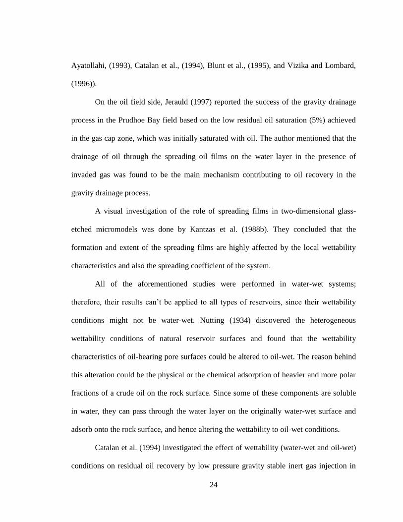
Figure 3.1: Geological map for the Arabian plates showing the location of Shaybah field.
Modified from Sharland et al. (2001) in Al-Ghamdi (2006) ................................................ 30
Figure 3.2: Three-D view of Shu’aiba reservoir superimposed on a picture of the Shaybah
field (Salamy et al., 2006) ..................................................................................................... 31
Figure 3.3: Simplified facies distributions of N-S cross-section (Al-Ghamdi, 2006) .................. 32
Figure 3.4: Simplified facies distributions of E-W cross-section (Al-Ghamdi, 2006) ................. 33
Figure 3.5: Core sample photographs of the lagoonal facies. Modified from Al-Ghamdi,
(2006) .................................................................................................................................... 34
Figure 3.6: Thin section photograph. Modified from Al-Ghamdi (2006) .................................... 35
Figure 4.1: Pore entry radii distribution versus incremental wetting saturation ........................... 42
Figure 4.2: Pore entry radii distribution versus cumulative wetting saturation ............................ 42
Figure 4.3: Air permeability versus median pore entry radii of selected samples ........................ 43
Figure 4.4: Low pressure curves of drainage capillary pressure of selected samples .................. 43
Figure 4.5: Drainage capillary pressure of selected samples ........................................................ 44
Figure 4.6: Schematic diagram of the USBM method for determining wettability (Zinszne
and Pellerin, 2007) ................................................................................................................ 51
Figure 4.7: Wettability index scale ............................................................................................... 52
Figure 4.8: T2 distributions of two carbonate plugs with low gas permeability ........................... 55
Figure 4.9: T2 distributions of two carbonate plugs with medium gas permeability .................... 56
Figure 4.10: Comparison between saturation porosity and NMR porosity .................................. 59
Figure 4.11: Gas permeability versus geometric mean of T2 for all selected samples ................. 60
Figure 4.12: Gas permeability versus geometric mean of the free fluid portion of T2 for all
selected samples .................................................................................................................... 61
Figure 4.13: Gas permeability versus standard deviation of the free fluid portion of T2 for all
selected samples .................................................................................................................... 61
Figure 4.14: Examples of beam hardening effects due to mineralogy ......................................... 65
Figure 4.15: Example of the CT scan image template used in this study ..................................... 67

xiii
Figure 4.16: Calibration of CT scanner using corrected density .................................................. 67
Figure 4.17: Comparison between CT scan porosity and routine porosity ................................... 68
Figure 4.18: Comparison between CT-porosity and CvCT ............................................................ 68
Figure 4.19: Heterogeneity characterization map of STD_T2FF versus CvCT ................................ 70
Figure 4.20: Typical CT-porosity distributions of the three heterogeneity groups ...................... 71
Figure 4.21: Typical NMR T2 distributions of the three heterogeneity groups ............................ 71
Figure 4.22: Poor correlation between predicted and measured permeabilities ........................... 75
Figure 4.23: Improved correlation between predicted and measured permeabilities ................... 76
Figure 5.1: Coreflood schematic used to conduct HPP gasflood experiments ............................. 78
Figure 5.2: The X-ray transparent coreholder used in this study .................................................. 82
Figure 5.3: The GE CTI CT scanner used in this study ................................................................ 83
Figure 5.4: Coreflood schematic for the LPP gasflood experiments ............................................ 87
Figure 6.1: Respective locations of the samples used in the centrifuge study .............................. 96
Figure 6.2: Oil recovery factor versus initial oil saturation from centrifuge ................................ 96
Figure 6.3: Relation between heterogeneity type and irreducible water from centrifuge study ... 97
Figure 6.4: Relation between heterogeneity type and total oil recovery from centrifuge study ... 97
Figure 6.5: Relation between heterogeneity type and remaining oil saturation from centrifuge
study ...................................................................................................................................... 98
Figure 6.6: Respective locations of the samples used to construct the LRH stack ..................... 104
Figure 6.7: Respective locations of the samples used to construct the MRH stack .................... 104
Figure 6.8: Respective locations of the samples used to construct the HRH stack .................... 105
Figure 6.9: LRH gasflood results from the LPP for the first gas injection period ...................... 106
Figure 6.10: LRH gasflood results from the LPP for the three gas injection periods ................. 107
Figure 6.11: MRH gasflood results from the LPP for the first gas injection period ................... 108
Figure 6.12: MRH gasflood results from the LPP for the three gas injection periods ............... 109
Figure 6.13: HRH gasflood results from the LPP for the first gas injection period ................... 110

xiv
Figure 6.14: HRH gasflood results from the LPP for the two gas injection periods .................. 111
Figure 6.15: Oil recovery characteristics of the three single heterogeneity rocks for the first
gas injection period ............................................................................................................. 116
Figure 6.16: Results comparisons between the three single heterogeneity rocks ....................... 116
Figure 6.17: NRF comparisons of the three single heterogeneity rocks for the first gas
injection period ................................................................................................................... 117
Figure 6.18: Pressure drop comparisons of the three single heterogeneity rocks for the first
gas injection period ............................................................................................................. 118
Figure 6.19: Oil saturation profiles (from CT scan) for the LRH rock (data accuracy: Swi
(±0.06%), Sorg1 (± 0.47%), Sorg2 (± 0.88%), and Sorg3 (±0.78%)) ....................................... 122
Figure 6.20: Oil saturation profiles (from CT scan) for the MRH rock (data accuracy: Swi
(±0.23%), Sorg1 (± 0.58%), Sorg2 (± 1.16%), and Sorg3 (±0.76%)) ....................................... 123
Figure 6.21: Oil saturation profiles (from CT scan) for the HRH rock (data accuracy: Swi
(±0.07%), Sorg1 (± 1.46%), and Sorg3 (±1.65%)) .................................................................. 124
Figure 6.22: NMR T2 distributions of the samples used to construct the MRH stack ................ 125
Figure 6.23: Respective locations of the samples used to construct the MIRH stack ................ 128
Figure 6.24: MIRH gasflood results from the LPP for the first gas injection period ................. 130
Figure 6.25: MIRH gasflood results from the LPP for the three gas injection periods .............. 131
Figure 6.26: Oil recovery characteristic for the LRH, MRH, HRH, and MIRH rocks............... 132
Figure 6.27: NRF characteristic for the LRH, MRH, HRH, and MIRH rocks ........................... 132
Figure 6.28: Oil saturation profiles (from CT scan) for the MIRH rock (data accuracy: Swi
(±0.18%), Sorg1 (± 0.92%), and Sorg3 (±1.31%)) .................................................................. 133
Figure 6.29: Respective location of the high permeability LRH sample .................................... 135
Figure 6.30: Comparison between the LPP’s gasflood results from the low and high
permeability LRH rocks ...................................................................................................... 136
Figure 6.31: Respective locations of the samples used to construct the HIRH stack for tertiary
gasflood ............................................................................................................................... 141
Figure 6.32: Results from secondary recovery mode (waterflood) ............................................ 142
Figure 6.33: Results from tertiary recovery mode (gasflood)..................................................... 143

xv
Figure 6.34: Bulk density (from CT scan) profiles for secondary and tertiary recovery modes
for MIRH rocks ................................................................................................................... 144
Figure 6.35: LRH gasflood results (HPP) ................................................................................... 147
Figure 6.36: MRH gasflood results (HPP) .................................................................................. 148
Figure 6.37: HRH gasflood results (HPP) .................................................................................. 149
Figure 6.38: Comparison between the three single heterogeneity rocks (HPP) ......................... 151
Figure 7.1: History matching results (LRH: LPP) ...................................................................... 154
Figure 7.2: History matching results (MRH: LPP) ..................................................................... 154
Figure 7.3: History matching results (HRH: LPP)...................................................................... 155
Figure 7.4: History matching results (MIRH: LPP) .................................................................... 155
Figure 7.5: History matching results (LRH-high perm.: LPP) ................................................... 156
Figure 7.6: History matching results (LRH: HPP)...................................................................... 156
Figure 7.7: History matching results (MRH: HPP) .................................................................... 157
Figure 7.8: History matching results (HRH: HPP) ..................................................................... 157
Figure 7.9: History matching results (MIRH-waterflood: LPP) ................................................. 158
Figure 7.10: Comparison between measured and matched results (LPP’s gasfloods) ............... 160
Figure 7.11: Comparison between measured and matched results (HPP) .................................. 161
Figure 7.12: Oil recovery factor versus initial oil saturation from all gasfloods ........................ 161

xvi
List of Symbols, Abbreviations and Nomenclature
Symbol Units Description
Ai - Frequency of an individual pore
AI Kg-1
Amplitude index
API - American petroleum institute
BET - Brunauer, Emmett and Teller
BPR - Back pressure regulator
BV m3 Bulk volume of a core sample
CIR m3/min Critical gas injection
CO2 - Carbon Dioxide
CPMG - Carr-Purcell-Meiboom-Gill
CT - Computerized Tomography
CTN - CT number
Cv - Coefficient of variation
CvCT - Coefficient of variation using CT data oC - Degrees Celsius
C1 - Methane
C4 - Butane
ECL - Exploration Consultants Limited
ECLIPSE - ECL’s Implicit Program for Simulation Engineering
EOR - Enhanced oil recovery
E-W - East to West
GAGD - Gas Assisted Gravity Drainage
GAIGI - Gas-assisted inert gas injection
GOR - Gas oil ratio
HPP - High pore-pressure
HRH - High rock heterogeneity
h m Thickness
IFT N/m Interfacial tension
IIR m3/min Initial injection rate
K-C - Kozeny-Carman
k m2
Permeability
ka m2
Air permeability
kb m2
Brine permeability
kh m2
Horizontal permeability
ko m2
Oil permeability at irreducible water saturation
kv m2
Vertical permeability
E - Mean
LPP - Low pore-pressure
LRH - Low rock heterogeneity
LC - Lorenz Coefficient
MIRH - Mixed rock heterogeneity
MMP Pa Minimum Miscibility Pressure
MME kg mol/m3
Minimum Miscibility Enrichment
MMm3/d - Million cubic meter per day

xvii
MRH - Moderate rock heterogeneity
MPR m Median pore-entry radius
MRC - Maximum Reservoir Contact
NaCl - Sodium chloride
NFR - Normalized recovery factor
NGLs - Natural gas liquids
NMR - Nuclear Magnetic Resonance
N-S - North to South
NC - Capillary number
N2 - Nitrogen
OOIP m3 Original oil in place
OR m3
Oil rate
PV - Pore volume
PVI pore volume Cumulative volume of gas injected
ROIP m3 Remaining oil in place
RPM - Rotation per minute
SCF - Standard cubic feet
STB - Stalk tank barrel
STD - Standard deviation
STD_T2FF s Standard deviation of the free fluid portion of the total T2 spectrum
So N/m Spreading coefficient
Sorw - Residual oil saturation to water
Sorg - Residual oil saturation to gas
SNMR m2
Total pores’ surface of a core sample from NMR
Swi - Irreducible water saturation
TIPM - Tomographic Imaging & Porous Media
T1 s Longitudinal relaxation time
T2 s Transvers relaxation time
T2FF s Free fluid portion of the total T2 spectrum
T2gm s Geometric mean of the total T2 spectrum
T2gm_FF s Geometric mean of the free fluid portion of the total T2 spectrum
T2, Bulk s T2 bulk relaxation
T2, Diffusion s T2 diffusion relaxation
T2, Surface s T2 surface relaxation
USBM - United States Bureau of Mines
Var -
Variance
VDP - Dykstra-Parson’s coefficient
VCS m2 Vertical cross-section
Vi m3
Volume of individual pore
ϕ - Porosity
ϕCT - CT porosity
ϕNMR - NMR porosity
ϕSAT - Saturation porosity
N/m Interfacial tension between gas and water
N/m Interfacial tension between gas and oil
N/m Interfacial tension between water and oil

xviii
Kg/m3 Density of water
Kg/m3 Density of oil
Kg/m3 Density of gas
Kg/m3
Grain density

1
Chapter One: INTRODUCTION
More than 60% of the world’s oil and 40% of the world’s gas reserves are found
in carbonate reservoirs (Schlumberger, 2013). The Middle East alone has about 62% of
the world’s proven conventional oil reserves (BP, 2007), where approximately 70% of
the reserve is found in carbonate reservoirs (Schlumberger, 2013). Two distinct carbonate
reservoirs of Cretaceous and Jurassic age, namely Arab-D and Shu’aiba reservoirs,
contribute heavily to the current conventional oil production in Saudi Arabia (Okasha et
al., 2005).
Saudi Arabia is promising to maintain the largest oil supply in the world
(Cordesman and Obaid, 2005). This has been translated into the development of more
reservoirs within the Kingdom. The Shu’aiba carbonate reservoir is considered a main
carbonate reservoir and has been under development since the mid-1990s. This reservoir
(~150 m thick) has a huge overlying natural gas cap (associated gas) and a weak
underlying aquifer (Al-Ghamdi, 2006; Al-Awami et al., 2005). The reservoir is marked
with a tight-facies formation with typical average permeabilities in the range of 10-40
mD. This mandated the use of horizontal wells as a development strategy such as
Maximum Reservoir Contact (MRC) wells to maximize reservoir contact, reduce gas
encroachment, and maintain desirable production rates (Saleri et al., 2003).
The current production practice in Shu’aiba reservoir is based on gas cap
expansion (pressure maintenance), where the produced gas (~25 MMm3/day) is
reinjected along with natural gas liquids (NGLs). However, very soon gas recovery could
be implemented in this reservoir (Cordesman and Obaid, 2005), which necessitates
finding an alternative gas (e.g. N2 or CO2). In this reservoir, oil is being immiscibly

2
displaced towards the producing wells located at the bottom of this reservoir. For gas to
displace oil towards a producing well, it needs to pass through different geologic-facies,
into which oil might be inefficiently or efficiently displaced.
Placement of wells (as a production optimization practice) could be considered a
key solution to maximize oil displacement efficiency in a composite heterogeneous
reservoir. However, the placement of wells into certain geological zones depends mainly
on the economic viability of such implementation. To test such economic viability,
consistent geologic reservoir models need to be established and then used in reservoir
dynamic studies to make reliable predictions of production performance for the reservoir
or individual wells, as spatial reservoir heterogeneity could change. This requires detailed
reservoir characterization practices including high quality reservoir data and
petrophysical properties such as porosity, permeability, capillary pressure, and relative
permeability. Furthermore, extensive experimental studies evaluating the effect of these
rock properties on oil recovery is essential.
In this research, the main objectives were to characterize the rock heterogeneity in
the studied cores based on the individual core sample’s permeability and porosity
variations using both NMR T2 and CT scan measurements, and carry out laboratory
experiments to evaluate the effect of this heterogeneity on oil recovery using both
unsteady state gasfloods and centrifuge drainage experiments. N2 gas, synthetic reservoir
brine, and crude oil (from Shu’aiba reservoir) were used as the gas and the liquid phases,
respectively.

3
In the heterogeneity classification method followed in this research, the core
samples in clean and dry conditions were first scanned using a CT scanner, after which
NMR T2 measurements on the brine saturated (2% NaCl) core samples were carried out
using an EcoTek-FTB low-field NMR machine. The magnitude of permeability and
porosity variations in an individual core sample are evaluated using the standard
deviation of the free fluid portion of the NMR T2 spectrum (STD_T2FF), and the
coefficient of variance of the CT number’s distribution (CvCT), respectively. The standard
deviation is a measure of dispersion of a set of data from its mean. The more spread apart
the data, the higher the deviation (Jensen et al., 2007). Samples with higher STD_T2FF
and CvCT would indicate high rock heterogeneity whereas samples with low STD_T2FF
and CvCT would indicate low rock heterogeneity. This variation in rock heterogeneity
could affect the oil recovery from immiscible gas injection due to oil trapping and/or
bypassing.
In a typical set of displacement runs (secondary gas injection mode), the core
sample was saturated with oil at irreducible water saturation, aged for a minimum of two
weeks, after which immiscible gas-oil drainage displacements were performed using
gasflood and centrifuge experiments. For tertiary gas injection mode, gas injection
commenced after reaching the ultimate oil recovery from waterflood. The measured oil
recovery to N2 gas injection would indicate if it were a function of rock heterogeneity
because in case of high rock heterogeneity, oil could be bypassed and/or trapped. This
could affect the total oil recovery from a reservoir or a certain formation in the reservoir
due to the displacement inefficiency caused by the rock heterogeneity.

4
Another objective of this work was to estimate the true oil recovery from
gasflooding by correcting for the effect of capillary end-effect using a black-oil lab
simulator. This was completed for all gasfloods performed in secondary gas injection
mode.
In the present study, Chapter Two lists the research objectives of this work.
Chapter Three reviews the literature relevant to the topics addressed in this research as
well as the historical background of the carbonate reservoir under study. In Chapter Four,
the results from wettability, mercury injection, and petrographic studies are discussed. In
addition, Chapter Four describes the method used to characterize the individual core
samples’ heterogeneity using NMR T2 and CT scan measurements. In Chapter Five, the
experimental apparatuses and procedures for immiscible gas-oil displacement
experiments are described. Chapter Six discusses the results from performing a series of
gas-oil drainage experiments from unsteady state constant injection rate and constant
injection pressure gasfloods as well as from single-speed centrifuge runs. In addition,
Chapter Six discusses CT scan results from the constant injection rate gasfloods. In
Chapter Seven, the results from conducting the simulation study (history matching) using
a lab simulator is discussed. Chapter Eight draws some conclusions and presents some
recommendations for further research.

5
Chapter Two: RESEARCH OBJECTIVES
The objectives of this research were to:
1. Select core samples for gas-oil displacement studies, and carry out various
core rock characterization studies like NMR, CT, wettability, Mercury
Injection, and Petrographic image analysis.
2. Construct a heterogeneity characterization map using NMR and CT in
order to classify selected samples’ heterogeneity into different
heterogeneity groups based on permeability and porosity variations within
a sample.
3. Develop a permeability-predictor model by linking the Kozeny-Carman
(K-C) empirical correlation to NMR T2 measurements and then test the
potential of this model against core samples under study.
4. Carry out unsteady-state drainage experiments (secondary recovery mode
operated at 1034 kPa and 80oC and under constant injection rate) using
restored-wettability samples to study the effect of single and mixed rock
heterogeneities on oil recovery using N2 gas and crude oil systems.
5. Undertake unsteady-state drainage experiments (secondary recovery mode
operated at 17237 kPa and 80oC and under constant injection pressure)
using wettability-preserved samples to study the effect of single rock
heterogeneities on oil recovery using N2 gas and live-oil systems.
6. Carry out unsteady-state drainage experiments (tertiary recovery mode
operated LPP and under constant injection rate) using restored-wettability

6
samples to study the effect of mixed rock heterogeneities on oil recovery
using N2 gas, reservoir brine, and crude oil systems.
7. Perform centrifuge drainage experiments using restored-wettability
samples to evaluate the effect of rock heterogeneity on the ultimate oil
recovery under favourable gravity drainage conditions.
8. History match the results from the secondary gasflood experiments
numerically to evaluate the magnitude effect of capillary end-effect and
estimate the true oil recovery.

7
Chapter Three: LITERATURE REVIEW
3.1 Depositional Textures and Diagenetic Processes
Sedimentation is the initial process forming a reservoir (e.g. sandstone and
carbonate). The production of carbonate sedimentations commonly takes place in warm
shallow oceans. This is caused by either direct precipitation from seawater or by
biological extraction of calcium carbonate from seawater to form skeletal material. The
result is sediment with particles of different sizes, shapes, and mineralogies. The mixing
of these components leads to different pore-size distributions (Lucia, 2007). The porosity
formed under these conditions is known as primary porosity (or depositional porosity).
In fact from the moment sediments are deposited, they experience physical,
chemical, and biological forces that define the type of rock they will become (Ali et al.,
2010). These post depositional alterations are known as diagenesis, which includes all the
processes that convert raw sediment to sedimentary rock (Worden and Burley, 2003).
Porosity and permeability are controlled by sediment composition and the conditions that
prevailed during deposition. However, after diagenesis commences they can be enhanced,
modified, or even destroyed (Ali et al., 2010).
This explains the degree of variation (heterogeneity) that can be seen in carbonate
rocks, where, at certain times, there is indirect relationship between porosity, for
example, and rock textures or fabrics. This lack of correlation indicates the complexity of
relating the heterogeneity in porosity and permeability to certain features or
environments. Despite this, it is still possible to classify porosity based on their rock
fabrics and textures.

8
3.1.1 Carbonate Porosity
Porosity is an important rock property and is a measure of the space available for
storage of fluids. In definition, porosity is the ratio of the pore volume of a porous
medium to its total volume (bulk volume).
Porosity in carbonate reservoirs ranges from 1% to 35% and is divided into two
types: primary and secondary porosities (Lucia, 1983). The primary porosity is formed
when sediment deposited and has two forms: interparticle and intraparticle porosities.
The interparticle porosity is often lost quickly in muds and carbonate sands through
compaction and cementation respectively. This porosity type retains and common in
siliciclastic sands. The intraparticle porosity is located in the interiors of carbonate
skeletal grains.
The secondary porosity in carbonate rocks is formed after deposition and has two
main forms dissolution and fracture porosities. The dissolution porosity is the typical
porosity of carbonate rocks. The fracture porosity is typically not voluminous, but is very
important because it can enhance permeability.
3.2 How has Heterogeneity been Classified in Carbonate Rocks?
Adapting more practical classification schemes can lead to more reliable
interpretations of pore systems. This is an important step for improving carbonate
reservoir management. Using classifications considering flow behaviour can help in
decision making during production operations (Ahr et al., 2005).
Different classification schemes have been used to study carbonate rocks (Scholle
and Ulmer-Scholle, 2003); the most common two classification methods used to classify
carbonate rocks are Dunham and Folk. The Dunham classification highlights depositional

9
textures, whereas the Folk classification starts with grain types and their relative
abundance, and then includes texture and grain size (Ahr et al., 2005). Other geologists
use classifications that emphasize pore properties to assess reservoir quality (Ahr, 2000).
The study of petrophysical rock types described by Archie (1950) is considered a
conceptual framework in siliciclastic and carbonate rock classification. This method
assumes rocks with common petrophysical types have comparable attributes such as
porosity, permeability, saturation, or capillary-pressure properties. Based on these
similarities, similar reservoir performance is expected.
Another approach to simplify carbonate heterogeneity is to apply the concept of
rock fabric and flow unit in order to relate different carbonate pore systems to
petrophysical properties (Lucia, 1983). The classification by Lucia (1983) predicts a
systematic relationship between permeability and porosity, and estimation of the water
saturation for the interparticle porosities. The concept of flow unit to improve the
prediction of flow performance was implemented by Wang et al. (1994) by simulation in
shallow-water reservoirs and also a carbonate ramp reservoir.
In order to develop a more accurate correlation between permeability and
porosity, Lonoy (2006) divided the pore system in carbonates into 20 sub-pore classes
and divided the genetic pore types such as interparticle, intercrysrtalline, and moildic
pore types (Choqutte and Pray, 1970) into patchy and uniform pore distributions. These
new pore systems are further subdivided into macro-,meso-, and micro-porosity based on
the dominating pore sizes.
Utilizing descriptive pore-system attributes advanced the effectiveness of
petrophysical rock types for permeability prediction in carbonate reservoirs. This can be

10
done by linking describable and mappable properties of carbonate rocks with geologic
models to improve quantitative analysis at a larger scale (Ahr, 2005). Understanding rock
types provides an important foundation for studying reservoir performance, but is not
enough to predict reservoir behaviour even in reservoirs that are not fractured (Ahr,
2005).
Another approach using mercury-injection capillary pressure has been
implemented to address the limestone pore systems in a giant carbonate reservoir (Ahr,
2005). Cappilary-pressure curves can be used to assess the flow in reservoirs (Wardlaw
and Taylor, 1976). The use of pore-system models that utilized porosity, permeability,
capillary pressure and relative permeability for each rock type helped to refine the
comprehensive reservoir model for this giant reservoir (Ahr, 2005).
Low field Nuclear Magnetic Resonance (NMR) is routinely used for carbonate
formation evaluation. However, measuring carbonate porosity, deriving permeability and
interpreting NMR data for pore-size distributions is more challenging, when compared to
sandstone. Nevertheless, this is exactly the type of information needed in formation
evaluation (Ahr, 2005).
The NMR spectrum from a fully saturated core sample is directly related to the
pore volume of this sample, which yields porosity. The similarity between pore-size
distributions obtained from NMR and pore-throat distributions obtained from mercury
injection is proven in some studies (Marschall et al., 1995), leading to the assumption that
pore body distributions can be used as an approximation for pore throat distributions by
multiplying by a constant (Mai and Kantzas, 2000). Thus, permeability can be predicted
from the NMR spectrum.

11
In addition, CT has been routinely used in reservoir rock characterization. This
technique provides a cross-sectional image representing a distribution of CT numbers.
These CT numbers are proportional to the rock density distributions within an image,
which can be interpreted to give porosity distributions. The routine use of CT is to aid in
sample selections for core flood experiments. However, CT as an accurate measurement
tool of porosity makes it a robust tool in studying porosity variation within different core
scales. Furthermore, CT can be used to investigate pore architecture in carbonate rocks
(Shafiee and Kantzas, 2009).
3.3 Statistical Characterization of Heterogeneity
In reservoir characterization, heterogeneity specifically applies to the variability
that affects flow (Jensen et al., 2007). Jensen et al. (2007) classified heterogeneity into
two measures, static and dynamic. Static measures of heterogeneity describe the
distribution in permeability and porosity of a given sample from the formation and
require some flow model to be used to interpret the effect of heterogeneity on flow
(Jensen et al., 2007).
Dynamic measures, on the other hand, are based on a flow experiment and are a
direct measure of how the variability affects the flow. The Dykstra-Parson’s coefficient
(VDP), the Lorenz Coefficient (LC), and the Coefficient of Variation (CV) are common
static measures of heterogeneity used in reservoir characterization (Jensen et al., 2007).
3.3.1 The Dykstra-Parson’s coefficient (VDP)
The VDP, introduced by Dykstra and Parsons in 1950, is more commonly used to
measure the variability in permeability. It can be defined in terms of the 16th
and 50th

12
percentile values of a log-normal permeability distribution as follows (Dykstra and
Parsons, 1950):
(3.1)
where k16 and k50 are the 16th and the 50th percentile values, respectively. When VDP = 0,
there is no variation in the permeability values with respect to location and the resulting
permeable medium is homogeneous. When VDP increases, the variation in the
permeability values increases and the permeable medium becomes more and more
heterogeneous. Jensen et al. (2007) argue that the LC offers several advantages over the
VDP; one of these advantages is that LC includes porosity heterogeneity and variable
thickness layers.
3.3.2 The Lorenz Coefficient (LC)
LC is one of the most commonly-used techniques for heterogeneity measurements.
The technique involves ordering the product of permeability and the representative
thickness ( kh) in descending order along with the corresponding porosity-representative
thickness product ( h ) for a well (or wells). The normalized cumulative values of kh ,
which is also known as the fraction of total flow capacity (between 0 and 1) are then
plotted against the normalized cumulative values of h , also known as the fraction of the
total volume (between 0 and 1). LC is calculated by multiplying the area between the
curve and a 45o line between [(0,0) and (1,1)] by two. LC can theoretically vary between
0 and 1, with 1 representing the highest degree of heterogeneity (Jensen et al., 2007).

13
3.3.3 Coefficient of Variation (Cv)
The coefficient of variation (Cv) is another lesser-known measure of
heterogeneity. It is a dimensionless measure of sample variability or dispersion and is
given by:
√
(3.2)
where the numerator is the sample standard deviation and the denominator is the sample
mean. For data from different populations, the mean and standard deviation often tend to
change together such that Cv stays relatively constant. Any large changes in Cv between
two samples indicate a dramatic difference in the populations associated with those
samples (Jensen et al., 2007).
3.4 Effect of Heterogeneity on Residual Oil from Waterflood
The effect of heterogeneity from pore scale to reservoir scale on residual oil
saturation to waterflooding has been proven to be significant (e.g. Wardlaw and Cassan,
1978; Wardlaw, 1980; Hanion et al., 1996). Different approaches have been considered to
investigate the magnitude effect of heterogeneity type such as pore-size distributions and
parallel heterogeneity (permeability) on residual oil to waterflood with earlier work
focused on waterflooding in layered systems with transverse communications
(Richardson and Perkins, 1957; Gaucher and Lindley, 1960).
In these studies, vertical cross-section (VCS) experiments using sand packs were
conducted. These studies reported that a low flow rate and mobility ratio increase oil
recovery. This is caused by gravity segregation and imbibitions of the water from the
coarse sand to the fine sand.

14
Vertical heterogeneity is the most common heterogeneity in sand stone reservoirs
where its effect on waterflood efficiency is well understood. However, heterogeneity in
carbonate reservoirs complicates the interpretation of its effect on residual oil saturation.
This is attributed to the great morphological complexity of carbonate rocks from pore to
field scale. The following literature review focuses on the effect of carbonate
heterogeneity on residual oil saturation to waterflood (Sorw).
Wardlaw and Cassan (1978) studied the effect of pore throat/pore size ratio on
Sorw of strongly water-wet sandstones and carbonate cores. Their results showed a
correlation between Sorw and pore throat/pore size ratio.
Wardlaw (1980) performed studies on the effect of pore size distribution on non-
wetting phase entrapment of strongly and intermediate wetted porous media. It was
shown that the geometric and topologic properties of a strongly wetted pore system
increases trapping of the non-wetting phase. Under the condition of the intermediate
wetting, pore geometry showed less effect on the non-wetting phase entrapment.
Chatzis et al. (1983), on the other hand, conducted waterflooding experiments
under water-wet conditions in random packs of equal spheres, heterogeneous packs of
spheres with microscopic and macroscopic heterogeneities and Berea sandstone. They
concluded the following:
1. Sorw values are independent of absolute pore size in system of similar pore
geometry.
2. Clusters of large pores accessible through small pores retain oil.
3. High aspect ratios tend to cause entrapment of oil.

15
Tjolsen et al. (1991) showed that the presence of rock heterogeneity and strong
laminations, found in the studied sandstone reservoir cores prevented flow in parts of the
core pore volume. This resulted in a broad variation of Sorw values in their cores.
MacAllister et al. (1993) conducted steady-state, water/oil, relative permeability
tests on a mixed-wet Baker dolomite (kabs = 110 mD, 22% porosity) core sample. Two
constant pressure drops of 27.6 kPa and 689.5 kPa were used to perform these tests.
Using CT, tests conducted at 27.6 kPa pressure drop showed that oil and water flow
occurred through separate macroscopic regions. This resulted in high relative
permeability in both phases. In the 689.5 kPa case, the relative permeability values were
lower because the saturation was more uniformly distributed. In addition, their results
showed that the saturation differences between the 27.6 kPa and 689.5 kPa cases were
significant for local saturation but less significant for the overall saturation.
deZabala and Kamath (1995) studied Sorw variations in dolomite carbonate rocks,
one with isolated vugs embedded in a porous matrix with high permeability (ka =
300mD, = 14%), and the other with isolated vugs embedded in a dense matrix with low
permeability (ka = 1mD, =11 %). Their results showed Sorw increases with increasing
pore-throat aspect ratio, and decreases with an increasing pressure drop across the core.
Hanion et al. (1996) presented a large number of waterflooding data of a giant
carbonate reservoir that showed large variations in Sorw values. This variation was
attributed to the variations in lithofacies as well as to individual core permeability within
a single lithofacie.
The effect of carbonate heterogeneity on Sorw was investigated by Kamath et al.
(2001), who used rock typing classification to divide the studied core into four different

16
rock types (kb = 6-85mD, = 17-26%), based on thin section and mercury injection data.
Their results revealed that cores with large pore-throat aspect ratio show the largest Sorw
value with the biggest variations as the pressure drop increased.
Waterflooding experiments in cores taken from 30 sandstone reservoirs with
different wettability conditions were conducted by Skauge and Ottesen (2002). Their
results showed that Sorw values in these cores vary from 4% to 45%, and that
intermediate-wet cores commonly showed the minimum Sorw values.
Masalmeh and Jing (2004) presented a special core analysis study in order to aid
in carbonate rock characterization and water-oil displacement modelling of a
heterogeneous reservoir. The porosity of the samples used in this study ranged from
about 27% to 30% and the permeability varied from 2 mD to 1000 mD. These samples
predominantly consist of grainstones and packstones. In this research, the authors
concluded that, for this particular reservoir, the Sorw did not show consistent correlation
with conventional rock typing or facies classification. This conclusion was reached since
the imbibitions’ capillary pressure showed significant variations for a set of samples
having similar permeability, porosity, and drainage capillary pressure curves.
Mitchell et al. (2004) studied the influence of heterogeneity on Sorw using two-
dimensional gamma rays imaging on slabbed carbonate core samples. The authors
concluded that heterogeneities in core samples disrupted waterflood fronts and could
generate localized extremes in Sorw during displacement processes.
The effect of pore structure, pore size distribution and rock textural on oil
recovery by waterflooding from two carbonate reservoirs of differing geologic ages was
investigated by Okasha et al. (2005). The pore size distribution of the Lower Cretaceous

17
(wackstone) reservoir is about 0.27 to 1.5 microns and 0.5 to 5.5 microns for the Late
Jurassic (limestone and dolomitic limestone) reservoir. The absolute air permeability for
the Lower Cretacous and Late Jurassic reservoirs ranges from 5.6 to 15.3 mD and 13.5 to
423 mD, respectively. Their results showed that the Sorw values from these reservoirs
were different. This variation was attributed to the variations of rock characteristics,
especially the relationship of textural and diagenetic features. Furthermore, their results
showed that, for the Late Jurassic rocks, as rock permeability increases, Sorw increases;
however, for the Lower Cretacous rocks, an opposite trend was seen.
Skauge et al. (2006) studied the effect of different pore classes on the recovery
factor from waterflood using carbonate cores selected from four different basins. This
research was based on single phase dispersion experiments where the measurements were
interpreted using the capacitance model developed by Coats and Smith (1964). Their
results showed that samples with high flowing-fraction of the pore-structure produced
high oil recovery.
The work of Pourmohammadi and Skauge (2008) focused on identifying the
most important single phase flow properties that may control waterflood efficiency, and
whether these single phase properties are sufficient, or if the pore class concept should be
included to predict recovery efficiency by waterflooding. The authors concluded that oil
recovery by waterflooding seems to be related to carbonate pore classes.
3.5 Effect of Reservoir Heterogeneity on Oil Recovery from Gas Injection
Gas injection (primarily CO2) is one of the most widely applied enhanced oil
recovery (EOR) methods (Agbalaka et al., 2008). Gas injection in either secondary or
tertiary recovery modes has proven successful in increasing oil recovery from both

18
sandstone and carbonate reservoirs. In the past two decades, gas injection with nitrogen
gas, flue gas, and enriched natural gas have also shown some beneficial results in
increasing oil recovery. Nitrogen and flue gas may be useful in areas where CO2 is not
economically available for use (Agbalaka et al., 2008).
The magnitude effect of reservoir heterogeneity on these recovery processes
varies depending mainly on miscibility conditions. The injection of gas horizontally in a
miscible condition as reported in previous studies (Brock and Orr, 1991, and Burger and
Mohanty, 1997) showed the importance of reservoir heterogeneity (layering and random
heterogeneity) on oil recovery. The immiscible gas injection process is also affected by
reservoir heterogeneity that commonly results in the channelling and bypassing of oil.
3.5.1 Effect of Rock Heterogeneity under Miscible Gas Injection
Oil recovery from gas injection can be very high when miscibility is achieved
between the gas and the oil (Rao, 2001). Miscibility can be achieved by applying
pressures equal to or exceeding the gas/oil Minimum Miscibility Pressure (MMP)
(Alston, 1985). This is also done by enriching the gas with components such as C1 to C4
hydrocarbons in concentrations equal to or greater than the Minimum Miscibility
Enrichment (MME) (Danesh, 1998). Achieving MMP in a reservoir is limited by the
reservoir pressure. Miscibility between the enriched gas and the oil, under MME, is a
function of mass transfer between the injected gas and the trapped/residual oil (Rao,
2001).
One of the key issues in miscible gas injection is bypassing. Bypassing usually
results from viscous fingering, gravity tonguing, channelling etc. The mobility ratio
controls the magnitude effect of viscous fingering and gravity tonguing. Channelling is
19
mainly caused by the magnitude heterogeneity in permeability. The following literature
summaries present few examples of studies investigating the effect of rock heterogeneity
on oil recovery from miscible gas injection.
Andrew et al. (1980) investigated the influence of rock characteristics on miscible
displacement behaviour by using a combination of displacement testing and modeling.
They conducted a number of stabilized CO2 displacements and tracer tests in both
outcrop sandstones and San Andres reservoir carbonate samples. Their results suggested
that microscopic heterogeneity is a primary determination of residual oil saturation to
miscible flooding when viscous fingering is controlled. Furthermore, their results from
both laboratory and model prediction showed that the effect of microscopic heterogeneity
is less important in field displacements than laboratory systems.
Newley and Begg (1992) conducted a simulation study to assess the impact of
small-scale heterogeneities on the vaporization by lean injected gas of residual oil
remaining in a gas cap after gas cap expansion. Their study considered two heterogeneity
reservoir elements, one with rapidly varying distribution of porosity and permeability and
the other with a more slowly varying distribution. They concluded that the small-scale
heterogeneities within a conventional simulation grid-block can have a significant impact
on the recovery of residual oil by lean gas injection.
Solano et al. (2001) conducted a simulation study to investigate the effect of
heterogeneity and capillary pressure on recovery of horizontal miscible-gas injection
process. The effect of heterogeneity was studied by varying the Lorenz coefficient (LC),
indicating heterogeneity in permeability. Their results showed that capillary pressure
increased oil recovery for LC less than 0.5 and reduced oil recovery for very

20
heterogeneous reservoir (LC greater than 0.6). Oil recovery decreased significantly with
increasing heterogeneity (LC greater than 0.6).
Variation in single phase fluid flow properties of different carbonate pore systems
from laboratory experiments was reported by Pourmohammadi et al. (2008). Their study
included eleven pore classes based on the Lonoy (2006) approach. In this study, the authors
studied the relationship between carbonate porosity systems and petropysical properties,
dispersivity, flowing-fraction and dead-end pores. Their results could aid in improving the
interpretation of oil recovery by a miscible displacement process for reservoirs with similar
pore classes.
Shedid (2009) studied the influence of different modes of reservoir heterogeneity
on performance and oil recovery of CO2 miscible horizontal flooding in carbonate
reservoir cores. The three considered modes of heterogeneity included single fracture
reservoirs (four different fracturing angles), layered rocks, and composite reservoirs
(different permeability configurations). His experimental results showed that all different
modes of reservoir rock heterogeneity have an important influence on oil recovery by
CO2 miscible flooding in carbonate oil reservoirs. It was also shown that higher oil
recovery was obtained from unfractured reservoirs than single fractured ones. It is to be
noted that the author’s results are specific to the rock-fluid combinations used in his
experiments.
Al-Wahaibi et al. (2009) conducted a simulation study using a compositional
simulation to investigate the effect of different geometries and permeability contrasts
within cross-bedded laminations on oil recovery from multicontact miscible gas injection.

21
Their results demonstrated that cross-bedding heterogeneities may have a significant
impact on oil recovery.
3.5.2 Effect of Rock Heterogeneity under Immiscible Gas Injection
Immiscible gas injection in secondary or tertiary (for EOR process) injection
modes involves the displacement of medium to heavy oils using gas as a separate
displacement phase. One of the limitations in immiscible gas injection is the high
tendency of the injected gas to bypass the oil, resulting in very poor sweep and
displacement efficiencies. Reservoir heterogeneity is considered one of the several
factors influencing the magnitude effect of bypassing such as gravity and viscosity
(viscous fingering effects).
Slack and Ehrlich (1981) investigated the efficiency of the simultaneous injection
of water and nitrogen to mobilize Sorw in Berea sandstone. Their results showed a
reduction of Sorw of up to 18% PV. Furthermore, the authors conducted a numerical
simulation of water-nitrogen flooding in real reservoir geometries to study the effects of
water-nitrogen ratio, kV/kh and permeability profile. They concluded that water-nitrogen
flooding is capable of recovering an appreciable fraction of Sorw.
Soroush and Saidi (1999) conducted vertical immiscible gas/oil displacements in
low permeability (1 mD) long carbonate core at different rates (above gravity stable) and
pressure below MMP. The authors concluded that the low permeability reservoirs can be
produced to about 70% of the oil in place by gas injection if the reservoir pressure is kept
sufficiently high, below MMP. Furthermore, their results showed that injecting gas even
at high injection rates could still produce over 60% of the oil in place. This led the

22
authors to conclude that applying similar injection conditions to low permeability
conventional reservoirs could still provide good results.
Egermann et al. (2003) conducted below MMP gas displacement efficiency
comparisons on two oil wet composite cores from a carbonate reservoir. The two
composite cores were selected from the same rock-type and showed porosity and
permeability values around 30% and 10 mD, respectively. The individual plugs of the
two composites also showed comparable mercury injection curves obtained on
neighbouring end pieces. In order to obtain a flow rather dominated by viscous forces, the
authors used a gas injection rate of 10 ml/hr. The secondary gasflood results from both
composites showed an excellent match in terms of oil recovery and gas breakthrough.
Kuo et al. (2010) performed a simulation study to investigate the effect of local
heterogeneity under capillary, viscous, and gravity displacement conditions. They used
the results from CO2/Brine steady state measurements conducted by Perrin and Benson
(2010), where CT scanning was used to measure the porosity profile and fluid saturation
distribution in a Berea sandstone core showing small-scale local heterogeneity. The
simulation included running steady state CO2/Brine displacement tests on a gridded core
with and without the local heterogeneity. Their results showed that the influence of the
local heterogeneity on average CO2 saturation was important when the flow was
dominated by the capillary force regime.
Gasflooding experiments on sandstone cores with permeability ranges from about
2 – 600 mD were conducted by Skauge et al. (1997) in vertical mode and at constant
differential pressure. Their results showed that the remaining oil saturation range from

23
about 20% to 50%, depending on core’s absolute permeability and applied differential
pressure.
Keat et al. (2010) studied the effect of different kV/kh, layers arrangement, and
different permeability (k) values with same kV/kh on oil recovery factor from GAGD (Gas
Assisted Gravity Drainage) process by using Schlumberger ECLIPSE 100. Their results
showed that for heterogeneous models, the lower kV/kh model yielded a higher oil
recovery factor, and for the models with same kV/kh the one with a decreasing-downward
k yielded a higher oil recovery factor.
3.5.3 Effect of Wettability
It is well known (Agbalaka et al., 2008) that wettability of the porous medium has
a profound effect on the reservoir production performance. For an accurate description
and analysis of any injection process, the rock/fluid interactions such as wettability have
to be properly taken into account. Wettability determines the relative affinity of the solid
surface for oil, water, or gas. It also defines the development of the wetting films. The
formations and thickness, along with the spreading films, play important roles in gravity
stable gas injection processes. This was evident in the pioneering experimental work by
Dumore’ and Schols (1974), where gravity drainage in a homogeneous water-wet rock
was found to be very efficient.
After 1974, numerous further studies were undertaken and confirmed that high
oil recovery factors are achievable in water-wet sandstone cores, bead packs, and sand
columns through both secondary and tertiary modes of oil recovery gravity drainage.
(Chatzis et al., (1988), Kantzas et al., (1988a), Dullien et al., (1991), Chatzis and
24
Ayatollahi, (1993), Catalan et al., (1994), Blunt et al., (1995), and Vizika and Lombard,
(1996)).
On the oil field side, Jerauld (1997) reported the success of the gravity drainage
process in the Prudhoe Bay field based on the low residual oil saturation (5%) achieved
in the gas cap zone, which was initially saturated with oil. The author mentioned that the
drainage of oil through the spreading oil films on the water layer in the presence of
invaded gas was found to be the main mechanism contributing to oil recovery in the
gravity drainage process.
A visual investigation of the role of spreading films in two-dimensional glass-
etched micromodels was done by Kantzas et al. (1988b). They concluded that the
formation and extent of the spreading films are highly affected by the local wettability
characteristics and also the spreading coefficient of the system.
All of the aforementioned studies were performed in water-wet systems;
therefore, their results can’t be applied to all types of reservoirs, since their wettability
conditions might not be water-wet. Nutting (1934) discovered the heterogeneous
wettability conditions of natural reservoir surfaces and found that the wettability
characteristics of oil-bearing pore surfaces could be altered to oil-wet. The reason behind
this alteration could be the physical or the chemical adsorption of heavier and more polar
fractions of a crude oil on the rock surface. Since some of these components are soluble
in water, they can pass through the water layer on the originally water-wet surface and
adsorb onto the rock surface, and hence altering the wettability to oil-wet conditions.
Catalan et al. (1994) investigated the effect of wettability (water-wet and oil-wet)
conditions on residual oil recovery by low pressure gravity stable inert gas injection in

25
Berea sandstone cores. They concluded that tertiary gravity drainage in water-wet
systems is most efficient in the case of positive spreading coefficient. In addition, in the
case of oil-wet systems, the authors reported very effective results.
Some experimental and numerical simulation studies investigating the role of
wettability conditions (water-wet, oil-wet, and heterogeneous-wet) on the oil recovery
from secondary gravity stable gas injection in sandpacks at irreducible water saturation
were also conducted (Vizika and Suquerroix, 1997). The heterogeneous-wet system
consisted of two long water-wet parts separated by a 2 cm thick oil-wet stratum. Their
results showed that the heterogeneous wettability dramatically affected the gas injection
process by drastically affecting phase distributions and displacement mechanisms.
Wylie and Mohanty (1998) investigated the effect of wettability on bypassing by
conducting gravity dominated secondary gas floods in Berea sandstone cores, under
slightly immiscible conditions. Their results showed that less bypassing occurs in a
strongly oil-wet system than in a water-wet system.
Pedrera et al. (2002) studied the effects of wettability on immiscible air gravity
drainage by conducting secondary mode experiments with varying core wettabilities.
Their results showed higher oil recoveries (64%) when oil-wet systems were used, when
compared to (52%) from water-wet systems.
Parsaei and Chatzis (2011) experimentally investigated the effect of wettability
heterogeneity at the macroscopic scale on the recovery efficiency of the gravity-assisted
inert gas injection (GAIGI) process, defined first by Kantzas (1988a), for tertiary
recovery of Sorw in unconsolidated glass beads. To construct the heterogeneous
wettability system, the authors embedded isolated inclusions of oil-wet consolidated glass

26
beads in a continuum of unconsolidated water-wet glass beads. Their results showed that
the Sorw was higher in the case of the heterogeneous-wet case when compared to the
water-wet case. However the recovery factor from the tertiary GAIGI process was higher
in the case of the heterogeneous-wet system which was attributed to the presence of the
isolated oil-wet inclusions. The final residual oil saturation was higher in the case of the
heterogonous-wet system as compared to the water-wet system because of the favourable
wettbaility condition in the water-wet case.
The above discussion obviously shows that the wettability influences on gravity
drainage are not very clear. Although the literature appears to be in agreement concerning
the beneficial effects of oil spreading and film flow in water-wet and mixed-wet systems,
confusing reports concerning the effects of wettability on gravity drainage recoveries in
oil-wet systems have been found.
3.5.4 Effect of Spreading Coefficient
The spreading coefficient, along with wettability, is believed to affect the gas-oil-
water distributions, which in turn affect oil recovery during a gas injection process. The
spreading coefficient is considered a balance between the three interfacial tensions (IFT)
in oil/water/gas systems, and defined as:
(3.3)
In addition to the reservoir wettability, the spreading coefficient value is critical in
determining the equilibrium spreading characteristics between the three co-existing
reservoir phases. The fluid spreading characteristics are critical in determining oil
recovery when gas injection is considered. In addition, the orientation and continuity of

27
the fluid phase in the reservoir pores is affected by the equilibrium value of the spreading
coefficient.
When oil (as continuous oil films) spreads over the water films covering the rock
grains, it increases the oil drainage phenomenon (during gas injection at lower pressure
drops) and provides continuous ‘conduits’ that aid in producing oil globules. This
continuity of oil films is caused by the interfacial phenomenon and depends on the ability
of the oil phase to spread on the water phase in presence of the gas. The spreading
coefficient can either be positive or negative depending on the fluids’ composition and
reservoir temperature and pressures.
Using micromodel experiments, Oren and Pinczewski (1994) visually
investigated the effects of wettability and fluid-fluid spreading on gas flood oil recovery.
Their results prove that the positive value of the spreading coefficient helps ensure
development and maintenance of continuous oil films between injected gas and reservoir
water. This resulted in minimal losses of the injected gas to the reservoir water. The
negative value, on the other hand, signifies a lens-type discontinuous distribution of oil
between water and gas. This enables gas-water contact and therefore lowers the oil
recovery.
Catalan et al. (1994) performed inert gas injection assisted by gravity experiments
on short core plugs with varying wettability and heterogeneity characteristics. The
authors concluded that tertiary gravity drainage is efficient when the oil can spread on
water in the presence of gas, in water-wet systems. Their experimental results also
suggested that the oil-wet nature of the porous medium did not negatively affect the oil
recovery factors.

28
Vizika and Lombard (1996) experimentally studied the effect of spreading and
wettability on gravity drainage oil recovery process in water-wet, oil-wet and
fractionally-wet porous media. Their results showed that in water-wet porous media, oil
recovery depends on the spreading coefficient value, while in oil-wet media the spreading
coefficient did not affect the process efficiency. Their results also showed that the highest
oil recoveries were obtained in water-wet and fractional-wet media under positive
spreading coefficient conditions. The oil recoveries were found to deteriorate when the
spreading coefficient value was negative. The authors used numerical simulation to
match the experimental results showing that the lowest oil recoveries were obtained in
oil-wet porous media. This was attributed to the capillary retention effect on the observed
continuous oil films.
3.5.5 Effect of Connate Water Saturation
Gas injection as a secondary recovery process is usually conducted at connate
(irreducible) water saturation. This connate water saturation is commonly assumed to be
immobile. However, the micromodel studies carried out by Sajadian and Tehrani (1998)
suggested that this assumption may not always hold true. Their research suggested that
changes in the gravity-capillary force balances (during gas gravity drainage) could result
in saturation redistributions and/or connate water re-mobilization during the process.
Dumore and Schols (1974) performed gravity stable gas displacement
experiments in high permeability oil saturated cores. Their results showed that the
presence of connate water saturation was critical for achieving very low residual oil
saturations during gravity drainage displacements.

29
Hagoort (1980) conducted centrifuge gravity drainage experiments using
consolidated outcrop and field cores. His results show that oil relative permeability
increased when initial water was present.
Gas gravity drainage (free and controlled) experiments in both Berea sandstone
and in unconsolidated sand columns of various lengths were conducted by Kantzas et al.
(1988b). Their results showed higher oil recoveries when the tests were started at initial
water saturation than when started at Sorw.
Skauge et al. (1994) also carried out gas gravity drainage experiments at different
water saturations in order to study the effect of water saturation on oil recovery. Their
results revealed that oil recovery by gas gravity drainage depends on the connate water
saturation, and that oil relative permeability increased with connate water present.
3.6 The Geological Description of the Reservoir under Study
The Shu’aiba Formation, Shaybah field, discovered in 1968 in the Rub’ al-Khali
desert of Saudi Arabia and developed by horizontal wells in 1996 (Figure 3.1), is a Lower
Cretaceous carbonate reservoir. This giant reservoir is about 64 km long by 13 km wide
and 150 m thick (Al-Ghamdi, 2006). The field is characterized as a gently folded (Figure
3.2) northeast-southwest trending anticline and has a number of faults (Salamy et al.,
2006). This giant field is producing oil and gas below a depth of around 1484 m (4900 ft)
(Hughes, 2000, in Al-Ghamdi, 2006). The oil in the Shu’aiba reservoir is Arabian Extra
Light with an average API of 42o and a gas-oil-ratio (GOR) of about 750 SCF/STB (Al-
Awami et al., 2005).
30
Figure 3.1: Geological map for the Arabian plates showing the location of Shaybah
field. Modified from Sharland et al. (2001) in Al-Ghamdi (2006)

31
Figure 3.2: Three-D view of Shu’aiba reservoir superimposed on a picture of the
Shaybah field (Salamy et al., 2006)
The Shu’aiba Formation is considered one of the main oil producers in the U.A.E,
Oman and Saudi Arabia (Alsharhan, 1995) and is known to be very heterogeneous in
terms of lithology and reservoir quality. This is due to the development of ruddist build-
ups that vary laterally into barrier and shelf slope facies (Alfaraj, 1998).
The Shu’aiba Formation is divided into 17 facies based on sediment types (Al-
Ghamdi, 2006). Simplified facies distributions of N-S and E-W cross sections are shown
in Figure 3.3 and Figure 3.4, respectively.
Core sample and thin section photographs of the Lagoonal facies (facies used in
the current study) are shown in Figure 3.5 and Figure 3.6, respectively.

32
Figure 3.3: Simplified facies distributions of N-S cross-section (Al-Ghamdi, 2006)

33
Figure 3.4: Simplified facies distributions of E-W cross-section (Al-Ghamdi, 2006)

34
(A) Fine skeletal peloidal packstone
(shallow lagoon)
(B) Agreipleura floatstone in fine skeletal
packstone matrix (shallow-intermediately
deep lagoon)
(C) Lime mudstone with chert (deep lagoon)
Figure 3.5: Core sample photographs of the lagoonal facies. Modified from Al-
Ghamdi, (2006)

35
(A) Fine skeletical peloidal packstone
(shallow lagoon)
(B) Dasyclad alga (Salpingoporella) in
fine skeletical packstone (moderately
deep lagoon)
Figure 3.6: Thin section photograph. Modified from Al-Ghamdi (2006)
Table 3.1: Summary of lagoonal lithofacies. Modified from Al-Ghamdi (2006)
The porosity in Shu’aiba reservoir is generally high, with an average of 25%, and
does not vary laterally. The permeability, on the other hand, is facies-dependent and
varies laterally and vertically. The average reservoir permeability in this reservoir is 13
mD. In south Shaybah, permeabilities range from 5 to 10 mD, whereas in the north the
matrix permeability ranges from 50 to 200 mD. The low permeability facies of Shu’aiba
reservoir (5 to 10 mD), such as the lagoon and lithocodium, represents 60% of the
Shu’aiba rock facies. The remaining 40% of the Shu’aiba facies has relatively high

36
permeabilities, with an average matrix permeability of about 50 mD (Salamy et al.,
2006).

37
Chapter Four: RESERVOIR ROCK CHARACTRIZATION
To achieve the main objectives of this work, cores under study are evaluated for
wettability characteristics, pore-size distributions, and thin section photographs.
Furthermore, by using the results from NMR and CT, a new characterization approach
classifying the rock heterogeneity in terms of porosity and permeability variations within
the scale of a core plug is established.
The following sections present the results from mercury injection, petrographic,
and wettability studies. In addition, this chapter describes the characterization approach
used in this study.
4.1 Sample Selection
A total of 51 core plug samples in dry condition were selected for this study.
These samples were selected from the same geological facies of four wells representing
the Lagoonal facies of the Shu’aiba reservoir in Shaybah field. The samples are about 3.8
cm in diameter and 5 cm in length and were cut horizontally every half-foot interval for
basic core analysis. These samples had been previously cleaned with toluene to remove
hydrocarbons and with methanol to remove residual salts. These samples were then dried
for 48 hours at 85oC. The dry samples were used in the LPP gasfloods and centrifuge
experiments. Several wettability-preserved samples (sister plugs of the dry plugs) were
selected and used in the reservoir conditions gasfloods.
An additional 12 wettability-preserved samples were selected from the same
interval of the dry plugs. These samples were used to evaluate the wettability
characteristics of this reservoir interval using both the Amott and the United States
Bureau of Mines (USBM) wettability evaluation methods.

38
Another five samples were selected in order to study the pore-size distributions in
this reservoir interval using mercury injection method.
4.2 Air Permeability and Porosity Measurements
Permeability to gas and porosity measurements were carried out on these samples
in Saudi Aramco Exploration and Production Advanced Research Center (EXPEC ARC),
Dhahran, Saudi Arabia. Porosity measurements were conducted using COREXPORT
Auto Porosimeter, and permeability measurements were carried out using a (KA-210)
Gas Permeameter manufactured by Coretest System, Inc. All testes were done at ambient
conditions of 1379 kPa confining pressure and room temperature. Porosity and air
permeability of all selected samples are listed in Table 4.1. Samples designated with “*”
superscript were used in the centrifuge study.

39
Table 4.1: Routine data of selected samples
4.3 Mercury Injection and Drainage Capillary Pressure Study
Seven samples were selected for mercury injection capillary pressure tests. These
tests were carried out using TerraTek System, which is a multi-sample automated
mercury injection system at EXPEC ARC, Dhahran, Saudi Arabia. This system is
configured with servo control of the injection pore pressure or volume displacement. It

40
measures the core sample’s response to test variables. The system also performs pore-size
and volume analysis of core samples.
This system is designed to inject mercury into large rock samples (3.81 cm in
diameter by 7.62 cm in length). It can operate at pressure up to 137,895 kPa. All tests
were performed up to a maximum mercury injection pressure of 102,731 kPa and
ambient conditions of room temperature and zero overburden pressure.
Pore entry (throat) radii and pore throat distributions are calculated from the
mercury injection data. Appendix A shows plots of incremental and cumulative wetting
phase saturation versus the pore entry radius for each sample. Figure 4.1 and Figure 4.2
present plots of incremental and cumulative wetting phase saturation versus the pore
entry radius for all samples. Hence, a volume increment injected is the volume accessible
through throats within a defined size range. These plots show that five samples exhibit a
unimodal distribution; while samples 3C and 5C show two distinguished peaks in pore
size (bimodal distribution). Such distributions may reflect a complex diagenetic history.
All samples have a small percentage of medium (> 1 micron) pores except
samples 3C and 5C. The median pore-entry radius (MPR) value for each sample is listed
in Table 4.2. Both Figure 4.2 and Table 4.2 indicate that the median pore values vary
from 0.51 to 2.23 microns. Figure 4.3 shows that air permeability is in a good agreement
with the MPR. This could indicate that, for these particular carbonate rocks, the pore size
distribution is a good permeability indicator.
Figure 4.4 and Figure 4.5 show the low pressure and the total pressure curves of
the drainage capillary pressure of all samples. This plot shows the closure pressure,
which is defined as the pressure at which mercury commences to occupy the actual pore
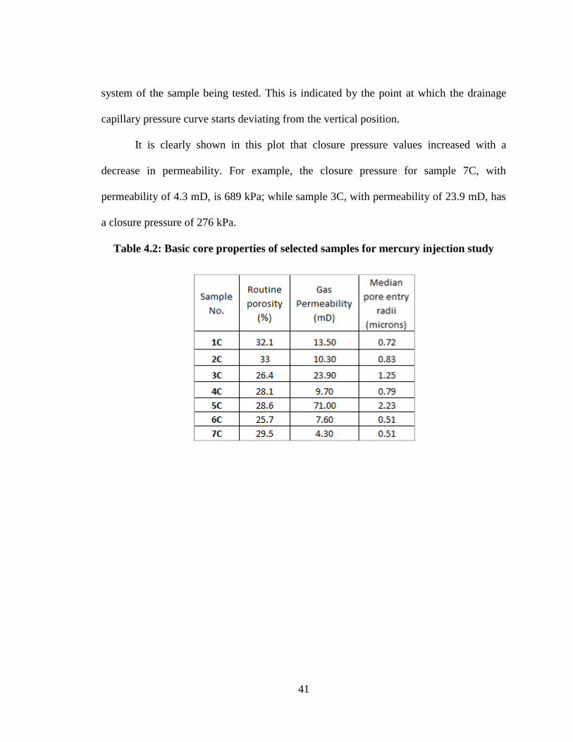
41
system of the sample being tested. This is indicated by the point at which the drainage
capillary pressure curve starts deviating from the vertical position.
It is clearly shown in this plot that closure pressure values increased with a
decrease in permeability. For example, the closure pressure for sample 7C, with
permeability of 4.3 mD, is 689 kPa; while sample 3C, with permeability of 23.9 mD, has
a closure pressure of 276 kPa.
Table 4.2: Basic core properties of selected samples for mercury injection study

42
Figure 4.1: Pore entry radii distribution versus incremental wetting saturation
Figure 4.2: Pore entry radii distribution versus cumulative wetting saturation

43
Figure 4.3: Air permeability versus median pore entry radii of selected samples
Figure 4.4: Low pressure curves of drainage capillary pressure of selected samples

44
Figure 4.5: Drainage capillary pressure of selected samples

45
4.4 Petrographic Study
Six samples were selected for the petrographic evaluation study, which was
conducted in the Petrophysics unit of EXPEC ARC, Dhahran, Saudi Arabia. The samples
represent the sister-plugs of samples 4, 5, 8, 16, 20, and 34 (Table 4.1). These samples
belong to the Agriopleura and Miliolid subfacies of the Shuaiba reservoir. Within these
subfacies, the samples are texturally classified as wackestones (Dunham, 1962).
Slices of these samples were obtained and used to make microscopic thin
sections. In order to make identification of the pore space easier, these thin sections were
prepared by vacuuming and pressure saturating with blue dyed epoxy. The samples were
examined using a McCrone BH-2 petrographic microscope and a binocular microscope.
A petrographic record of each sample was made.
Table B. 1, Appendix B.1, presents a summary of the findings of this evaluation
study. The plates were shot at 4 magnifications. Plates 1, 3, 5, 7, 9, and 11 (Figure B. 1,
Figure B. 3, Figure B. 5, Figure B. 7, Figure B. 9, and Figure B. 11) are thin section
photomicrographic of the samples. The “A” designated photos in these plates have a
magnification of 51x, and all were shot under plane light. The alpha-numeric scale
surrounding the photos has a scale of 103 microns/division.
The “B” designated plates were also shot under plane light, and have a
magnification of 107x. The surrounding scale for the “B” photos is 49.3
microns/division.
Plates 2, 4, 6, 8, 10, and 12 (Figure B. 2, Figure B. 4, Figure B. 6, Figure B. 8,
Figure B. 10, and Figure B. 12) are photos taken by a binocular microscope in order to
show the texture of these samples. The “A” designated plates have a magnification of

46
6.2x, with a scale of 700 microns/division. The “B” designated plates have a
magnification of 22.5x, and a scale of 200 microns/division. In the following discussion,
all comments concerning porosity relate to visual percent volume.
Sample 1T, the sister plug of sample 20 in Table 4.1, geologically belongs to the
Lagoonal/Agriopleura-pellet Wackestone category (Plates 1A to 2B in, Figure B. 1 and
Figure B. 2). This sample is composed texturally from 70% mud, and 30% grains. Its
primary porosity has been preserved in many of the biogenic fragments (Plate 1A: A28,
M22), and as original inter-granular porosity (Plate 1A: F14, Q4). Some remnant pelloids
can be seen (Plate 1B: K18, O6), generally between 6 and 90 microns in diameter. The
fine-grained mud matrix contains significant qualities of biogenic debris. The largest pore
bodies are approximately 50-90 microns. The fine grain matrix results in large amounts
of micro-porosity (10 microns or less). The visual porosity in this sample shows a
relatively uniform distribution.
Sample 2T, the sister plug of sample 4 in Table 4.1, geologically belongs to the
Lagoonal/Agriopleura Wackestone category (Plates 3A to 4B in Figure B. 3, and Figure
B. 4). The dominant porosity in this sample is primary micro-porosity, which was
developed in the inter-granular mud matrix. Secondary porosity was developed through
dissolution of biogenic fragments (Plate 3A: H15, J26; Plate 3B: H22, G27; in Figure B.
3), which show residual calcite rims. Furthermore, secondary micro-porosity was
developed through dissolution of the mud matrix. Some secondary porosity has been lost
to precipitation of calcite in the dissolution pores (Plate 3B: U23, E11, D27; in Figure B.
3). The calcite is probably locally sourced by a pressure solution at grain-grain contacts
in the mud matrix.

47
This sample shows that approximately 30% of the originally developed secondary
porosity appears to have been lost to re-precipitation of the calcite. The diagenetic
sequence has developed a complex pore structure of moderate heterogeneity. Pore throats
are small (5-15 microns), but the pores are well interconnected. Plate 4B, in Figure B.4,
shows a typical example of dissolution of a biogenic fragment, and re-precipitated calcite
(L15, R18) filling a portion of the diagenetic pore. The sample is 75% lime mud and 25%
biogenic grains and fragments. Approximately, 13% of the total porosity is micro-
porosity.
Sample 3T, the sister plug of sample 8 in Table 4.1, geologically belongs to the
Lagoonal/Agriopleura-pellet Wackestone category (Plates 5A to 6B, in Figure B. 5, and
Figure B. 6). This sample is very similar to sample 2T. The dominant porosity in this
sample is primary micro-porosity developed in the inter-granular mud matrix. Secondary
porosity was developed through dissolution of biogenic fragments (Plate 5A: O25; H13)
which show residual calcite rims. In addition, secondary micro-porosity was developed
through dissolution of the mud matrix.
There is abundant evidence of re-crystallization of the lime mud. Some secondary
porosity has been lost to precipitation of calcite in the dissolution pores (Plate 6B: E25).
Approximately 15% of the originally developed secondary porosity appears to have been
lost to re-precipitation of the calcite. The diagenetic sequence has developed a complex
pore structure, of moderate heterogeneity. Pore throats are small (5-15 microns), but the
pores are well interconnected. This sample is 60% lime mud and 40% biogenic grains,
fragments and pellets. The micro-porosity represents approximately10% of the total
porosity in this sample.

48
Sample 4T, the sister plug of sample 16 in Table 4.1, geologically belongs to the
Lagoonal/Agriopleura-pellet Wackestone category (Plates 7A to 8B, in Figure B. 7, and
Figure B. 8). This sample is composed of about 40% lime, 30% deformable pelloids, and
30% biogenic fragments. Porosity in this sample has been developed through dissolution
of the biogenic fragments (Plate 7A: H9, A19, S21; in Figure B. 7). The fragments
commonly have well developed calcite rims. Secondary micro-porosity is developed
through re-crystallization of the mud matrix (Plate 7A: D10, H3; in Figure B. 7).
Approximately 12% of the porosity in this sample is micro-porosity. The sample
demonstrates a bi-modal distribution. In terms of pore structure, this sample is more
heterogeneous than sample 1T, and the pores are well interconnected. The pore throats
are somewhat larger than sample 1T.
Sample 5T, the sister plug of sample 5 in Table 4.1, geologically belongs to the
Lagoonal/Agriopleura-pellet Wackestone category (Plates 9A to 10B, in Figure B. 9, and
Figure B. 10). The sample shows considerable inter-granular porosity, which appears to
be secondary as a result of dissolution of the lime mud matrix. This resulted in a complex
pore structure of high heterogeneity, and a high level interconnection between the pores.
There has been significant recrystallization of the remaining matrix. Although a large
amount of lime mud has been dissolved, the sample retains the mud-supported structure
indicative of a wackestone.
The remaining material shows relic pellets (Plate 9A: G25, N13) and biogenic
debris (Plate 11B: O10). There is little secondary precipitation of calcite in the pores,
which indicates that the dissolved material was mobilized after dissolution, and not re-
precipitated as in most of the samples in this study.

49
Sample 6T, the sister plug of sample 34 in Table 4.1, geologically belongs to the
Lagoonal/Miliolid Wackestone category (Plates 11A to 12B, in Figure B. 11, and Figure
B. 12). This sample is dominated by the mud matrix. Micro-porosity represents over 24%
of the total porosity of the sample, which resulted from dissolution of the mud matrix.
The biogenic fragments represent about 10% of the total sample. Though these biogenic
fragments were dissolved earlier in diagenetic history, they were refilled calcite (Plate
11A: B14, N20, S10; in Figure B. 11).
The low permeability of the mud matrix made it impossible for the dissolved
calcite to move out, so it precipitated in the available porosity. This sample shows re-
crystallization of portions of the mud matrix, as with the previous samples. Some relic
80-100 micron pelloids can be seen in this sample (Plate 11A: M28, J12; in Figure B.
11), but they represent a minor portion of the assemblage.
Authigenic pyrite was noted in this sample, which may be the result of reduction
of sulphur compounds in organics (possibly related to worm burrows or other biogenic
activity). The pore structure in this sample is homogenous, but dominated by very small
pore throats. A large portion of the permeability of this sample was almost certainly lost
to the secondary precipitation of the calcite.
4.5 Wettability Characterization Study
The term wettability refers to the preference of the rock surface for one or the
other of two immiscible fluids. The Amott and the USBM methods are used to measure
wettability as quantitative tests. Both of the Amott and the USBM methods were used in
this study to evaluate the wettability characteristics of the cores under study.

50
4.5.1 Wettability Study using the Amott and the USBM Methods
Seven wettability-preserved core plugs were selected and used to study the
wettability characteristics of the reservoir’s interval under study using the Amott method.
These tests were carried out at EXPEC ARC, Dhahran, Saudi Arabia. These samples
were first flushed to establish irreducible oil saturation. After that, oil imbibition (static
and dynamic) was determined, and followed by water imbibition (static and dynamic).
Amott wettability indices were calculated based on comparison of the spontaneous and
dynamic imbibition volumes of the aqueous and oleic phases (Amott, 1959). At the
conclusion of testing, samples were extracted and dried to measure core properties.
An additional five wettability-preserved core plugs were selected and used to
study the wettability characteristics of these cores using the USBM method. These tests
were carried out in EXPEC ARC, Dhahran, Saudi Arabia using centrifugation equipment
developed by Exxon Production Research Company. Testing was performed through a
procedure described by Slobod et al. (1951) and Donaldson et al. (1969). Core plugs were
subjected to centrifuge drainage and imbibition cycles. Each cycle consisted of six
displacement speeds ranging from 450 to the maximum speed of 2400 RPM. The volume
of each fluid displaced at each speed (oil or water) was observed through the top of the
centrifuge by means of transparent lid (a stroboscope) and calibrated collection tubes. All
tests were run using a confining pressure of 10342 kPa and 66 oC.
The USBM method uses the ratio of areas under the two capillary pressure curves
(Figure 4.6) to calculate indices according to the following equation:

51
(
⁄ ) (4.1)
where,
WI = wettability index
A1 = area under drainage curve
A2 = area under imbibition curve
Figure 4.6: Schematic diagram of the USBM method for determining wettability
(Zinszne and Pellerin, 2007)
The wettability index (WI) range of +1.0 to -1.0 was divided and classified as
follows: neutral (+1.0 to -0.1), slightly water-wet (+0.1 to +0.3), water-wet (+0.3 to 1.0),
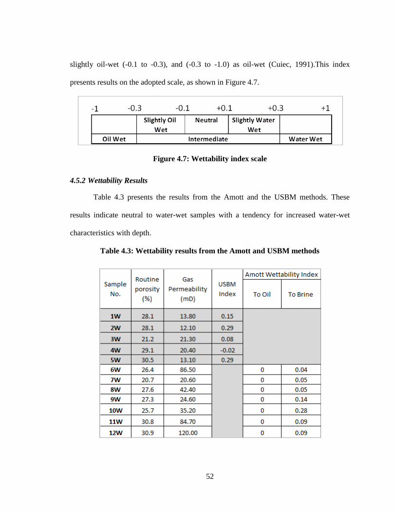
52
slightly oil-wet (-0.1 to -0.3), and (-0.3 to -1.0) as oil-wet (Cuiec, 1991).This index
presents results on the adopted scale, as shown in Figure 4.7.
Figure 4.7: Wettability index scale
4.5.2 Wettability Results
Table 4.3 presents the results from the Amott and the USBM methods. These
results indicate neutral to water-wet samples with a tendency for increased water-wet
characteristics with depth.
Table 4.3: Wettability results from the Amott and USBM methods

53
4.6 Characterization of Porosity and Permeability Variation within a Plug Scale
The new approach used in this study integrates the results from both NMR and
CT scan in order to classify the variations in porosity and permeability within a plug
scale. The following section presents an overview of the use of NMR to evaluate
permeability variations within a core plug, and CT scan to assess porosity heterogeneity
within a core plug.
4.6.1 Use of NMR as Permeability Variation Indicator
NMR was first introduced to the petroleum industry with the work of Brown and
Fatt in 1956. Their pioneering laboratory work used measurements of the T1 relaxation
rate to characterize pore size and wettability.
NMR is based on the simple principle that protons in a permanent magnetic field
can temporarily store radio frequency energy. The rate at which the protons lose this
stored energy can be monitored and recorded with a suitable radio frequency receiver.
The decay rates of the signal are referred to as the T1 (spin-lattice) or T2 (spin-spin) decay
times, and are based on phenomenological descriptions of the decay process.
The low-field NMR T2 measurements, made on water-saturated cores, provide a
view of the pore system based primarily on the relaxation of nuclear spins at the pore
surface, and can be used to measure total porosity and extract T2 distributions. This
mechanism provides data that can be used to correlate with permeability. The correlation
with permeability is based on the close relationship between NMR T2 distributions and
pore-size distributions (Straley et al., 1997).
Current models for the relaxation process and the corresponding permeability
transform are based on the equations first proposed by Bloembergen et al. (1948).

54
[
] (4.2)
and,
⁄ (4.3)
where,
T2 = Transverse relaxation time
SR = Surface relaxivity
S/V = Surface to volume ratio
The S/V ratio is used as the physical basis for the permeability transform.
Generally, the permeability is assumed to increase as the S/V decreases (Siddiqui et al.,
2000). Physically, NMR measurements are exponentially decreasing alternating currents.
To characterize the pore system in a reservoir rock, the exponentially decreasing signal is
inverted into a distribution of exponentials (T2 times), which are considered to
correspond to specific pores (or S/V ratios).
Samples with broader NMR T2 distributions might indicate large variation in
permeability within the core scale, when compared to others with narrower NMR T2
distributions. This difference in NMR T2 distributions might not essentially lead to
different average permeabilities for both cases; it solely describes the variation in
permeability within these samples. For example, Figure 4.8 and Figure 4.9 shows NMR
T2 distributions of two carbonate samples having almost identical average air
permeability. Samples designated with “A” are used in this study whereas the ones
designated with “B” are taken from another carbonate reservoir.

55
As can be seen from these figures, samples taken from reservoir “B” have broader
T2 distributions than samples taken from reservoir “A”, which indicates a broad
distribution of pore sizes in reservoir “B” samples. Though air permeability of each pair
samples is almost identical, it can be postulated from their NMR spectra that the two
phase flow outcomes from these samples will be different.
Figure 4.8: T2 distributions of two carbonate plugs with low gas permeability

56
Figure 4.9: T2 distributions of two carbonate plugs with medium gas permeability
4.6.1.1 NMR Experimental Work and Data Analysis
The NMR work completed in this part involves conducting low-field NMR T2
measurements on all 51 core samples assuming full saturation condition is achieved.
NMR measurements were conducted using an EcoTek-FTB low-field NMR
relaxometer (available at PERM Inc. and TIPM Laboratory, Calgary), which was
manufactured by the EcoTek Corporation. This machine operates at a frequency of
around 1.8 MHz, and measures samples at ambient temperature and pressure. NMR
measurements were made using a CPMG pulse sequence with the parameters listed in
Table 4.4.

57
Table 4.4: NMR parameters used in this study
The samples were vacuumed for 24 hours, and then saturated with degassed brine
(2% NaCl). These samples were then left to soak for additional 24 hours under vacuum.
Prior to testing, the samples were wrapped with Teflon tape, and inserted in a Ziploc bag
to minimize core desaturation during testing. After the conclusion of each test, the sample
bulk volume was measured using the Archimedes method.
It is known that the NMR response is a time delay signal that can be used
independently to characterize the pore space. However, the NMR response is more
frequently inverted to fit what is referred to as distributed exponential fit. This distributed
exponential fit is called a T2 distribution and serves as the basis for core sample
interpretation of NMR. Although several techniques exist to invert the time domain decay
curve to a T2 distribution, the one most commonly used is based on the Butler et al.
(1981) algorithm. This procedure is incorporated in the program ExpFit (developed by
PERM Inc. and TIPM Laboratory, Calgary), which was used to obtain the T2
distributions of all samples. These T2 distributions are presented as amplitude frequency
(A) versus time (T2, ms).
The NMR T2 distribution represents a distribution of pore-volumes. This
distribution of pore-volumes is commonly divided into two portions: bound fluid and free
fluid portions. This can be achieved by fixing a T2 value, known as T2cutoff , that separates

58
the two fluid portions. It is widely accepted that the T2cutoff value varies with lithology,
especially within carbonate rocks (Mai and Kantzas, 2000). In this study, a T2cutoff value
(121 ms) was chosen based on the experience with these carbonate rocks (Rose et al.,
2003). However, a T2cutoff value (125 ms) was used in this work since the output T2 bins
from ExpFit doesn’t show 121 ms.
NMR-porosity of each sample was evaluated using the following equation:
(4.4)
where, AT = total NMR amplitude of fully saturated core (-)
AI = amplitude index of brine (Kg-1
)
= density of brine (Kg/m3)
BV = bulk volume of core (m3)
The amplitude index (AI) of brine is defined as the total amplitude (AT) of the
brine sample with known mass.
(4.5)
where, = mass of brine (Kg)
The T2 geometric mean ( ), the T2 geometric mean of the free fluid portion
(defined as the portion carrying the producible fluids [Brown and Neuman, 1980])
( ), and standard deviation of the free fluid portion (STD_T2FF) of T2 distributions
were evaluated using Equation (4.6) and Equation (4.7), respectively.
[∑
] (4.6)
and,

59
[ √∑ ( (
))
∑
]
(4.7)
The porosity obtained from NMR is compared with the saturation porosity in
Figure 4.10. It can be seen that NMR-porosity is fairly accurate compared to the same
saturation porosity. This means that NMR T2 distributions can be trusted and used for
further investigations.
Figure 4.10: Comparison between saturation porosity and NMR porosity
The use of statistics (mainly the T2 geometric mean and standard deviation of T2
distribution) to describe permeability variations within a core sample is based on the
assumption that T2 distribution is an analogy of pore-size distribution. In order to
describe permeability variations in each core sample, the STD_T2FF is obtained for each
core plug.

60
Figure 4.11 through Figure 4.13 plot , and the STD_T2FF against
core gas permeability. Figure 3.8 shows that permeability increases as the of the
total spectra increases. However, when the T2gm-FF is plotted against core permeability
(Figure 4.12), the correlation and scatterings of the data improved. This indicates that the
average pore-size of the free fluid pores (T2gm-FF) is a more representative factor of the
average core permeability, when compared to the of the total spectra.
Figure 4.11: Gas permeability versus geometric mean of T2 for all selected samples

61
Figure 4.12: Gas permeability versus geometric mean of the free fluid portion of T2
for all selected samples
Figure 4.13: Gas permeability versus standard deviation of the free fluid portion of
T2 for all selected samples
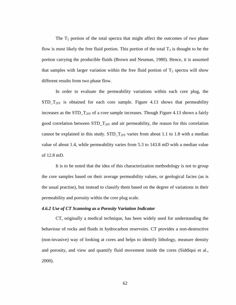
62
The T2 portion of the total spectra that might affect the outcomes of two phase
flow is most likely the free fluid portion. This portion of the total T2 is thought to be the
portion carrying the producible fluids (Brown and Neuman, 1980). Hence, it is assumed
that samples with larger variation within the free fluid portion of T2 spectra will show
different results from two phase flow.
In order to evaluate the permeability variations within each core plug, the
STD_T2FF is obtained for each core sample. Figure 4.13 shows that permeability
increases as the STD_T2FF of a core sample increases. Though Figure 4.13 shows a fairly
good correlation between STD_T2FF and air permeability, the reason for this correlation
cannot be explained in this study. STD_T2FF varies from about 1.1 to 1.8 with a median
value of about 1.4, while permeability varies from 5.3 to 143.8 mD with a median value
of 12.8 mD.
It is to be noted that the idea of this characterization methodology is not to group
the core samples based on their average permeability values, or geological facies (as is
the usual practise), but instead to classify them based on the degree of variations in their
permeability and porosity within the core plug scale.
4.6.2 Use of CT Scanning as a Porosity Variation Indicator
CT, originally a medical technique, has been widely used for understanding the
behaviour of rocks and fluids in hydrocarbon reservoirs. CT provides a non-destructive
(non-invasive) way of looking at cores and helps to identify lithology, measure density
and porosity, and view and quantify fluid movement inside the cores (Siddiqui et al.,
2000).

63
When an object such as a core plug is CT scanned, focused beams from an X-ray
source penetrate the object and the emergent beams are captured by a set of detectors. At
each scan location, the X-ray source and detectors move around the object to cover the
entire 360 degrees. The mathematical algorithm used in CT scanning reconstructs the
object by comparing the attenuation of the X-ray beams going through and coming out of
the object.
The attenuation of the energy in the X-ray beams is related to the electron density
and atomic number of the materials present in the object being scanned. Each material
possesses a distinct linear attenuation coefficient and the total response received by the
detectors is a combination of these coefficients. A normalized scale (of attenuation
coefficients) known as the CT number is generally used for computational purposes. In
typical laboratory scanning conditions, the CT number varies linearly with the bulk
density of core materials.
The porosity of a core plug can be determined by means of CT number. One way
to do this involves scanning standards of known bulk densities and plotting bulk density
versus CT numbers. The slope and the intercept of the straight-line fit are then used to
compute the bulk density ( ) of the unknown samples. Once the bulk density is
known, porosity at each volume element (voxel) can be calculated using the following
equation:
(4.8)
and,
(4.9)

64
where,
= density of matrix (2710 kg/m3, for limestone)
= density of matrix and fluid filling pores (kg/m3)
= density of fluid filling pores (kg/m3)
= CT number (-)
= Average voxel porosity (-)
4.6.2.1 CT Scanning Experimental Work and Data Analysis
The CT scanning work completed in this part involves scanning a total of 51 core
samples under dry conditions. This step is required for characterization purpose.
In order to use CT scan as a quantitative and a qualitative tool, typical laboratory
scanning conditions are required. These include diminishing if not eliminating the X-ray
artefact, known as “beam hardening”, and selecting the proper standard materials (used
for calibration).
Beam hardening effect is commonly seen in CT image slices containing higher
density core materials (e.g. dark yellow or green in Figure 4.14). This beam hardening
does not represent the true density value in the affected areas and usually CT data from
these areas are excluded from analyses. One way to reduce this artefact (during CT
scanning) is using “X-ray filtering” materials such as plastic and aluminum. A
combination of a plastic tube (Peek, 2.54 cm in thickness), and an aluminum tube (1.27
cm in thickness) were found to be suitable for the carbonate rocks used in this study.

65
Figure 4.14: Examples of beam hardening effects due to mineralogy
The standard materials used in this research are listed in Table 4.5 with their
corresponding bulk densities.
CT scan experimental work was conducted at U of C in Calgary, using a GE CTI
scanner manufactured by General Electric. The main CT scan parameters used for these
purposes are 120 kV, 100 mA, 0.1-cm beam thickness, and 0.2-cm scan interval.
Appendix C shows CT scan qualitative results of all core plugs compiled in a
template as depicted in Figure 4.15.
Figure 4.16 presents a plot of corrected standard bulk density ( )
versus the corresponding CT number. The slope and the intercept of the straight-line fit
are then used to compute the bulk density ( ) of the samples under study.
The bulk densities of these samples were then converted to average voxel porosities. This
results in a CT-porosity distribution and an average CT-porosity value for each core
sample.

66
Figure 4.17 shows a good match between porosities measured using gas
expansion and the ones obtained from CT scan. This justifies using CT data in describing
porosity variations of the carbonate core samples used in this study.
The use of statistics to compare slice-by-slice density or porosity data obtained
from CT provides an effective way to describe heterogeneity in each core sample
(Siddiqui et al., 2006). The typical statistical data generated by CT are the mean, standard
deviation, and minimum and maximum CT number.
In order to describe porosity variations in each core sample, the average of the
(described in Section 2.3.3) of CT numbers for each slice was obtained. Figure 4.19
shows the scatterings of ’s with respect to porosity of the core samples. vary
from about 0.03 to 0.09 with a median value of about 0.05, while porosity varies from
23.7 to 35.6 % of BV with a median value of 30.5 % of BV. There is no unique
relationship between and porosity data for these samples.
Table 4.5: Standard material used for CT calibration
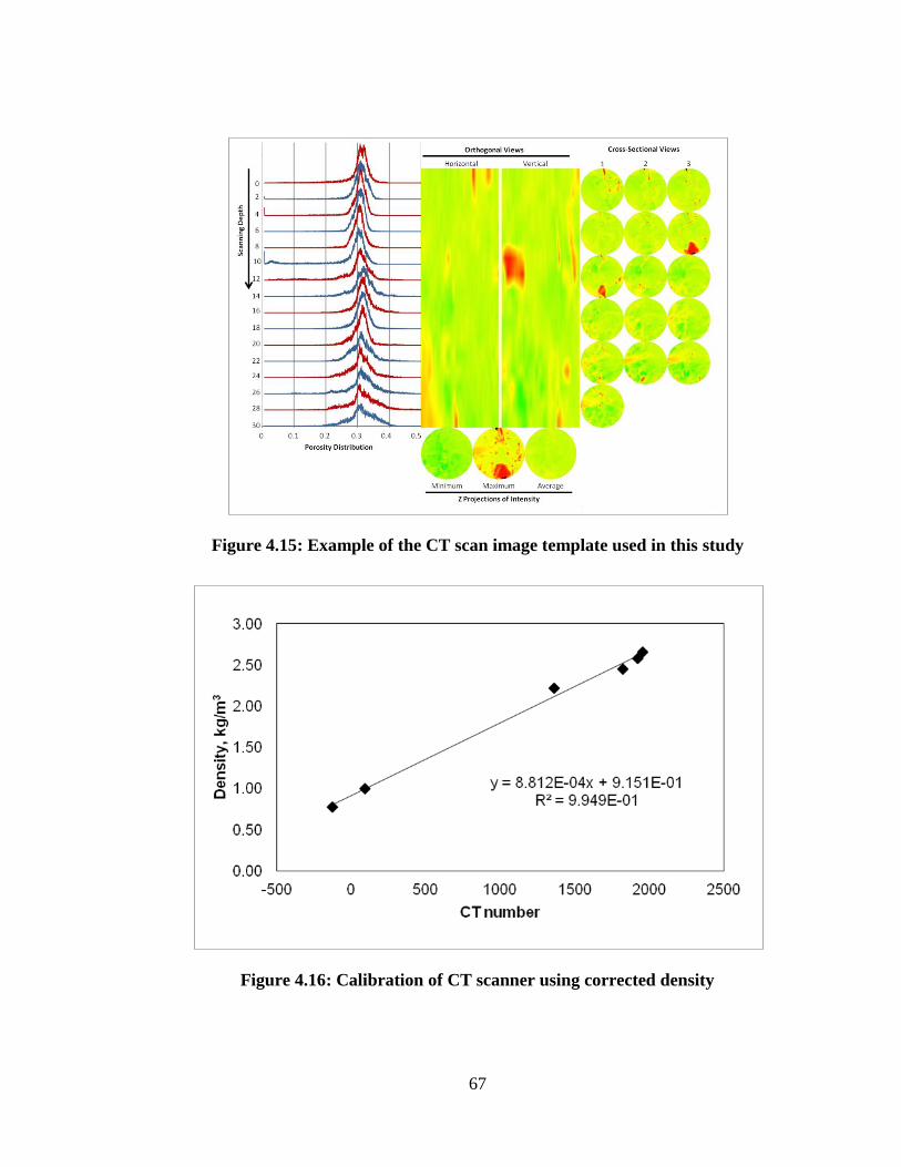
67
Figure 4.15: Example of the CT scan image template used in this study
Figure 4.16: Calibration of CT scanner using corrected density

68
Figure 4.17: Comparison between CT scan porosity and routine porosity
Figure 4.18: Comparison between CT-porosity and CvCT
4.6.3 Combining NMR and CT Results
This section demonstrates the attempts to group these carbonate core plugs based
on the degree of variation in their permeability and porosity within the plug scale. This
work identifies heterogeneity map for a group of carbonate samples.
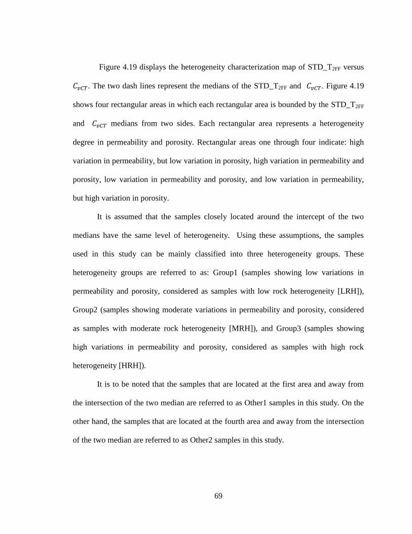
69
Figure 4.19 displays the heterogeneity characterization map of STD_T2FF versus
. The two dash lines represent the medians of the STD_T2FF and . Figure 4.19
shows four rectangular areas in which each rectangular area is bounded by the STD_T2FF
and medians from two sides. Each rectangular area represents a heterogeneity
degree in permeability and porosity. Rectangular areas one through four indicate: high
variation in permeability, but low variation in porosity, high variation in permeability and
porosity, low variation in permeability and porosity, and low variation in permeability,
but high variation in porosity.
It is assumed that the samples closely located around the intercept of the two
medians have the same level of heterogeneity. Using these assumptions, the samples
used in this study can be mainly classified into three heterogeneity groups. These
heterogeneity groups are referred to as: Group1 (samples showing low variations in
permeability and porosity, considered as samples with low rock heterogeneity [LRH]),
Group2 (samples showing moderate variations in permeability and porosity, considered
as samples with moderate rock heterogeneity [MRH]), and Group3 (samples showing
high variations in permeability and porosity, considered as samples with high rock
heterogeneity [HRH]).
It is to be noted that the samples that are located at the first area and away from
the intersection of the two median are referred to as Other1 samples in this study. On the
other hand, the samples that are located at the fourth area and away from the intersection
of the two median are referred to as Other2 samples in this study.

70
Figure 4.19: Heterogeneity characterization map of STD_T2FF versus CvCT
Figure 4.20 shows typical CT-porosity distributions of samples representing the
three heterogeneity groups. The NMR T2 distributions of these samples are depicted in
Figure 4.21. The locations of these samples on the heterogeneity characterization map
(Figure 4.19) are indicated.
Figure 4.20 shows that the sample with low heterogeneity in permeability and
porosity exhibits a relatively narrower CT-porosity distribution than the sample with high
variation in permeability and porosity. In addition, this sample exhibits a narrower (uni-
model) NMR T2 distribution, whereas the sample with high variations in permeability
and porosity shows a broader (approximately, bio-model) NMR T2 distribution (Figure
4.21).
Appendix C presents CT-porosity and NMR T2 distributions for all selected
samples, except some that were erroneously deleted from a personal computer.
1
3 4
2

71
Figure 4.20: Typical CT-porosity distributions of the three heterogeneity groups
Figure 4.21: Typical NMR T2 distributions of the three heterogeneity groups
4.6.4 Will this Rock Heterogeneity affects the Capillary Based Production Process?
Now that the heterogeneity in these cores has been classified, it is useful to
forecast the effect (i.e. neutral or negative) of this heterogeneity on the capillary based
production process. One possible way to test this effect is by predicting the permeability

72
in these cores using the well-known permeability correlation (Kozeny-Carman [K-C]).
The K-C has been proven to work well for homogenous porous medium (Peng Xu, 2008),
where all pores are very well inter-connected and porosity is inter-granular-porosity.
Since this work investigates carbonate cores, one main existing problem is the
pore connectivity (mainly between large and small pores). If using the K-C produces a
good match with the absolute permeability of these cores, then it is likely these cores will
yield less effect on the capillary based production process due to pore connectivity. If a
poor match is revealed, then the capillary production process will probably be more
affected by the connectivity issue in these cores.
In order to predict permeability using the K-C and NMR response, a certain link
has to be established. The established link between the K-C and NMR is basically
through the total surface area of pores to the bulk volume of the system (S/V) ratio. Using
this link, different K-C based NMR empirical correlations were developed (Seevers,
1966; Kenyon et al., 1988).
In this study, a very simple form of the K-C (Equation (4.10)) (Gates, 2011)
correlation was used, into which the NMR T2 response was incorporated through the use
of the total pores’ surface area (SNMR) of a sample. This correlation has the following
form:
(4.10)
where “S” is the interstitial surface, defined as the total surface of the pores divided by
the bulk volume of the porous medium (Gates, 2011). The bulk volume (BV) of an

73
individual core plug was used in this correlation (measured using the Archimedes
method). Equation (4.10) then becomes:
(
)
(4.11)
The total surface of the individual core plug’s pores was estimated using NMR T2
response as follows:
∑ (
)
(4.12)
where,
Saturation porosity
Surface to volume ratio of an individual pore
Frequency of an individual pore
Amplitude index, defined in Equation (4.5)
can be written as:
(4.13)
By placing Equation (4.13) into Equation (4.12), Equation (4.12) becomes:
∑
(4.14)
This shows that the total pores’ surface of a core sample can be estimated using Equation
(4.12). Consequently, Equation (4.3) can be substituted into Equation (4.12) with the
assumption that is constant within a core sample. Equation (4.12) then becomes:

74
∑ (
)
(4.15)
The surface relaxivities for a set of samples selected from the same interval as
the studied cores were measured using the Brunauer, Emmett and Teller (BET) gas
adsorption technique. The individual plugs’ surface relaxivities were scattered in the
range of 1.30-4.78 µm/s.
The total surface area of the individual core plug was estimated using Equation
(4.15). The porosity used in the K-C correlation was measured using saturation method.
The Klinkenberg-permeability was matched against the predicted permeability based on
the K-C correlation. In the beginning of predicting the permeability, the average surface
relaxivity (3.04 µm/s) of the measured samples was used. Poor matching was obtained
between the measured and the predicted permeabilities (Figure 4.22). Consequently,
different average surface relaxivities (based on tested samples intervals) were used for the
samples from the same interval and are listed in Table 4.6. This step improved the match
between the measured and predicted permeabilities (Figure 4.23).
The good match between the measured and predicted permeabilities suggests that
this heterogeneity in these specific cores has good pore-to-pore connectivity. As a matter
of fact, the thin-section study indicated that a sample from the most heterogeneous
samples showed a good connectivity between its pore systems, suggesting that this type
of heterogeneity can even work in the capillary based production process.

75
Table 4.6: Average surface relaxivities used to improve the K-C correlation
Figure 4.22: Poor correlation between predicted and measured permeabilities

76
Figure 4.23: Improved correlation between predicted and measured permeabilities

77
Chapter Five: EXPERIMENTAL APPARATUS AND PROCEDURE
This chapter presents the apparatuses used in this study, details the procedure
used to conduct the gasflood experiments, and explains the method followed to analyse
CT scan data.
Two coreflood apparatuses were used in this study. The first coreflood apparatus
(EXPEC ARC, Saudi Aramco, Saudi Arabia) was designed by CoreTest Systems2, Inc to
conduct gas-liquid displacement experiments under high pressure/high temperature
conditions, while the second gasflood apparatus was assembled in house to carry out gas-
liquid experiments under low pressure/moderate temperature conditions.
5.1 EXPEC ARC Coreflood Apparatus
The coreflood apparatus used in this study was designed to investigate two-phase
flow behaviour under simulated reservoir conditions (80oC and 10,342 kPa net
overburden pressure). This apparatus consists of four main components:
Injection system
Coreflood cell
Production system
Data logging system
The detailed components of this gasflood system are shown in .
5.1.1 Injection System
The injection system consists of a dual cylinder Quizix pump. These pumps,
placed inside a split oven designed to maintain reservoir temperature, supply distilled
water to the bottom of floating piston accumulators filled with the desired fluids. Two
floating piston accumulators are used in this study to deliver dead-oil and live-oil. A gas
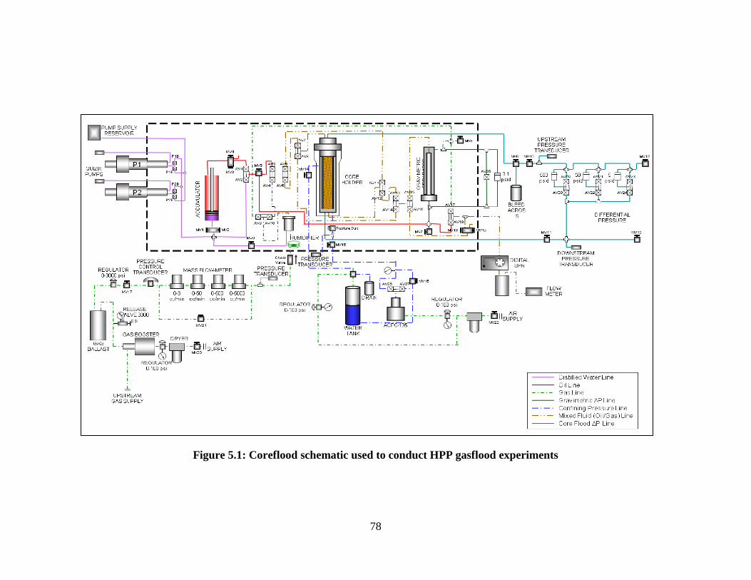
78
Figure 5.1: Coreflood schematic used to conduct HPP gasflood experiments

79
booster is placed outside the split oven and is used to boost N2 pressure to the desired
pressure. A gas-ballast and a pressure-controller are used to stabilize N2 pressure. Four
individual gas flow meters, in the range of 0-5, 0-50, 0-500, and 0-5,000 cm3/min (at
standard conditions), are used to measure gas flow rate. A humidifier vessel is placed
inside the split oven and is used to humidify N2 prior to injection into the core.
5.1.2 Coreflood Cell
The coreflood cell used in this study is a hydrostatically loaded core holder that
accommodates 3.81 cm in diameter cores up to 30.5 cm in length. The core stack is
placed in a Nitrile rubber sleeve with both ends secured to end plugs and a confinement
pressure of 10,342 kPa above operation pressure. An automated confining pressure
controller is used to maintain constant confinement pressure through all phases of the test
including system heat up. Three individual differential pressure transducers, in the range
of 0-34, 0-344, and 0-3447 kPa, are used to monitor differential pressure across the core.
5.1.3 Production System
Produced gas and oil are separated in a gravimetric separator, where the produced
liquid volume is measured. The produced gas exits the separator and goes through a
digital back pressure regulator. The atmospheric gas enters a glass separator where it is
cooled and any excess liquid is collected. The ambient condition gas volume is measured
with a gas flow meter totalizer.
5.1.4 Data Acquisition System
Different components of the system are monitored and controlled by the data
acquisition system (developed by CoreTest Systems2 Inc.). The data acquisition collects

80
raw data such as mass flow meter readings, produced gas and oil volumes, pore and
confining pressures, differential pressures, and system temperature.
5.2 In-House Coreflood Apparatus
The coreflood apparatus used in this study was designed to investigate certain
parameters and meet the research objectives. It was assembled in-house to serve as low
pressure/moderate temperature medium where desired condition fluid flow displacements
take place. This apparatus consists of four main components:
Injection system
Coreflood cell
Production system
Data logging system
X-ray computed tomography scanner
Table 5.1 provides a description of all components used in coreflood experiments.
The GE CTI X-ray computed tomography scanner (CT scanner) is used as a separate
component to map final fluid saturations during the coreflood experiments (saturation
and gasflood).
5.2.1 Injection System
The injection system consists of two dual cylinder Quizix pumps. These pumps
supply distilled water to the bottom of floating piston accumulators filled with the desired
fluids. Three floating piston accumulators are used in this study to deliver oil, brine, and
N2.

81
5.2.2 Coreflood Cell
The coreflood cell used in this study is shown in Figure 5.2. It is an x-ray
transparent core-holder made from peek plastic material. This core-holder can withstand
a maximum confinement pressure of 8274 kPa at 80oC. It accommodates 3.81 cm
diameter cores up to 30.5 cm in length. The core stack is placed in a Nitrile sleeve with
both ends secured to end plugs and a confinement pressure of 5,860 kPa above operation
pressure. The confinement pressure is maintained by a dual cylinder Quizix pump. The
coreflood temperature is maintained at 80oC by using a fixable heating tape that is set to
the desired temperature via a temperature controller. The core-holder cell is wrapped with
an insulation material to maintain constant temperature.
5.2.3 Production System
Produced fluids go through a dome type back pressure regulator (BPR) where the
pressure is set to the desired value by applying N2. Effluent fluids from BPR go through a
graduated glass collector where liquids remain while the atmospheric gas is vented from
the collector’s top. The atmospheric gas enters a glass separator where it is cooled and
any excess liquid is collected. The ambient condition gas volume is measured with a gas
flow meter totalizer.
5.2.4 Data Acquisition System
Different components of the system are monitored and controlled by the data
acquisition system (developed by TIPM Laboratory). The data acquisition system collects
raw data such as injected and produced gas volume, pore and confining pressures,
differential pressures, and system temperature.

82
5.2.5 The GE CTI X-Ray CT Scanner
Shown in Figure 5.3 is the GE CTI X-ray computed tomography scanner (CT
scanner). This CT scanner is used as a separate component to profile final fluid
saturations during coreflood course. It can be operated at different levels of power (up to
140 kV, and 200 mA).
Table 5.1: A list of equipment used in the in-house study
Figure 5.2: The X-ray transparent coreholder used in this study
Equipment Description
Quizix pumps Model 6K-SS, capacity 0.001 – 50 ml/min
Floating Piston Accumulators In-house machined, capacity 500 ml, max. pressure 10, 000 psi
BPR Dome type, max. pressure 3000 psi
Pressure Transducers Validyne, differential pressure, 10, and 50 psid
Gas Totalizer OMEGA, Model FMA-4302
Heating Tape OMEGA, Model SRT 101-040
Thermocouples OMEGA, J-type
Temperature Controller ZESTA, Model ZCP466
Equipment Information

83
Figure 5.3: The GE CTI CT scanner used in this study
5.3 Testing Procedure
This section provides the experimental steps followed during the experiments. It
is divided into three sections: HPP corefloods, LPP corefloods, and centrifuge
experiments which explain the fluid flow experiments.
5.3.1 Coreflood Experiments Performed at HPP
Shown in Figure 5.1 the complete coreflood system used to conduct all gasflood
experiments on wettability-preserved samples operated at 17237 kPa and 80oC. All tests
were conducted at 80oC, 17,237 kPa operating pressure, and 10,342 kPa net overburden
pressure. It is equipped with an auto data acquisition system, dual cylinder Quzix pumps,
and a hydrostatically loaded core holder. The main steps followed to conduct a gasflood
test are:
1. Trim and smooth selected samples to make cylinder plugs, then measure
individual plug’s dimensions.

84
2. Load the selected core plug in a Hassler type core holder with 5,516 kPa net
confining pressure and flush with at least two pore volumes of degassed brine
against 1,379 kPa back pressure to insure complete initial liquid saturation.
3. Measure brine permeability at atmospheric outlet pressure.
4. Spin the brine saturated samples inside a centrifuge (Mistral 3000) at 3000 RPM
for four hours in order to establish irreducible water saturation.
5. Repeat step two in order to saturate the selected core plug with dead-oil at
irreducible water saturation.
6. Mount the core plugs in the hydrostatically loaded core holder. In this process,
stack selected samples starting from the highest permeable core followed by the
lowest permeable core (based on brine permeability), and follow this order to the
end of the core stack. Use filter-paper to insure capillary continuity between core
plugs.
7. Flush the core stack with few pore volumes of dead-oil until the pressure drop
across the core stabilizes, and then measure oil permeability.
8. Age the core stack for one month. In this step, flush the core stack with fresh
dead-oil daily until the pressure drop across the core is stabilized.
9. Flush the core stack with several pore volumes of live-oil until the pressure drop
across the core stabilizes and then measure oil permeability.
10. Start N2 injection at constant injection pressure. In this step, stop N2 injection
when oil production remains constant for three readings.
11. Cool down the coreflooding system to room temperature, and then dismount the
core stack.

85
12. Measure end point saturations using Dean/Stark solvent extraction technique.
5.3.2 Coreflood Experiments Performed at LPP
Shown in Figure 5.4 the complete coreflood system used to conduct all gasflood
experiments on wettability-restored samples operated at LPP. All tests were conducted at
80oC, 1,034 kPa operating pressure, and 5,860 kPa net overburden pressure. It is
equipped with an auto data acquisition system, dual cylinder Quzix pumps, and an X-ray
transparent core holder. The main steps followed to conduct a gasflood test are:
13. Trim and smooth selected samples to create cylinder plugs, then measure
individual plug’s dimensions.
14. Mount the core plugs in the core holder. In this process, stack selected samples
starting from the highest permeable core followed by the lowest permeable core,
and follow this order towards the end of the core stack. Use filter-paper to insure
capillary continuity between core plugs.
15. Measure gas permeability (using Nitrogen) and porosity (helium expansion) of the
core stack.
16. Vacuum the core stack from both ends under temperature (80oC) for about 12
hours. After that, open inlet valve while closing outlet valve in order to saturate
the core stack with CO2 under constant injection pressure for about six hours.
Then, open outlet valve to flush out CO2 for few PVs, and close outlet valve to
continue CO2 saturation for additional four hours. Lastly, vacuum the core stack
from both ends for one day.
17. Mount core-holder horizontally and CT scan the core stack to obtain cross-
sectional images of 0.1 cm in thickness with 0.1cm spacing.

86
18. Saturate the core stack with degassed reservoir composite brine. The saturation is
accomplished by injecting brine into the core at constant pressure (345 kPa)
vernight.
19. Inject 3 to 4 PVs of brine with back pressure of 1379 kPa to ensure complete
saturation. Measure brine permeability and calculate the core stack’s PV using
material balance. Confirm the results with helium expansion and CT scan
calculations of the dry core.
20. Leave the core stack to reach temperature equilibrium overnight, and then CT
scan using same CT parameters of the dry core.
21. Saturate the core stack with reservoir crude oil to reduce the water saturation to
irreducible water saturation (Swi). This is accomplished by injecting five to seven
PVs of oil or until no further brine is produced.
22. Age the core stack for two weeks. In this step, flush the core stack with fresh oil
every five days until the pressure drop across the core is stabilized.
23. CT scan using same CT parameters of the dry core.
24. Mount the core holder vertically.
25. Start injecting Nitrogen at a constant rate. When no further oil is produced, stop
injecting gas, mount the core-holder horizontally, and then CT scan the core
stack.
26. Start injecting Nitrogen at constant rate higher than the previous rate. When no
further oil is produced, stop injecting gas, mount the core-holder horizontally, and
then CT scan the core stack.

87
27. Start injecting Nitrogen at constant rate higher than the second rate. When no
further oil is produced, stop injecting gas, mount the core-holder horizontally, and
then CT scan the core stack.
28. Cool down the core holder to room temperature, and then dismount the core stack.
29. Clean the core plugs from oil and salts using Dean-Stark.
Figure 5.4: Coreflood schematic for the LPP gasflood experiments
5.3.3 Centrifuge System
This experimental work was conducted to evaluate the ultimate oil recovery under
centrifuging conditions. This experimental work was carried out at an international
service lab (Intertek, USA).

88
The detailed experimental procedure followed to conduct the reservoir
temperature centrifuge work is:
1- Measure porosity and gas permeability.
2- Saturate samples with degassed composite brine using displacement with back
pressure, and then measure brine permeability at outlet atmospheric pressure.
3- Establish irreducible water saturation for samples by spinning in the centrifuge
inside oil-filled cups at centrifuge speed of 6000 RPM, and then measure Swi by
material balance.
4- Age samples for two weeks at a temperature of 80oC.
5- Flush samples with dead-oil by displacement with back pressure for a few pore
volumes and then measure ko at reservoir temperature (80oC).
6- Perform single-speed centrifuge (with camera system) oil relative permeability at
reservoir temperature (80oC) at 4000 RPM, using nitrogen as a displacing fluid,
which is achieved by purging the centrifuge-cup with nitrogen prior to running the
test.
7- Calculate Sorg using material balance.
8- Measure gas (nitrogen) permeability at Sorg , using the lowest acceptable gas flow
rate at 80oC.
9- Dean-Stark for end point saturations.
5.4 CT Scan Data Analysis Used in this Study
The output data from an X-ray machine is known as CT number (CTN). This
number is dimensionless and is mainly gives information concerning density. A very
popular approach in the literature (Akin and Kovscek, 2003) is to analyse CT scan data in

89
order to obtain information concerning fluid saturations within a core. This method
directly uses the raw data from CT scan (CTN), commonly used to obtain voxel-by-voxel
porosity (Akin and Kovscek, 2003) and is an explicit way to analyse CT data. To use this
method, the core needs to be scanned dry, saturated with water, saturated with oil at
irreducible water saturation, and at certain PVs flooded with a displacing fluid (e.g.
water). This can be achieved using the following equations:
for calculating porosity,
(5.1)
for calculating oil saturation (Rangel-German and Kovscek, 2002) ,
(5.2)
where,
= CTN of water (0)
= CTN of air (-1000)
= CTN of used oil
= CTN of rock saturated with water
= CTN of the rock in dry condition
= CTN of the rock after flooding with certain PVs
= CTN of the rock saturated with the resident fluid (e.g. water or doped water)
It is clear that this approach is based on a slope of two points (air and water). This
slope of air and water is measured on objects with relatively low densities. By assuming
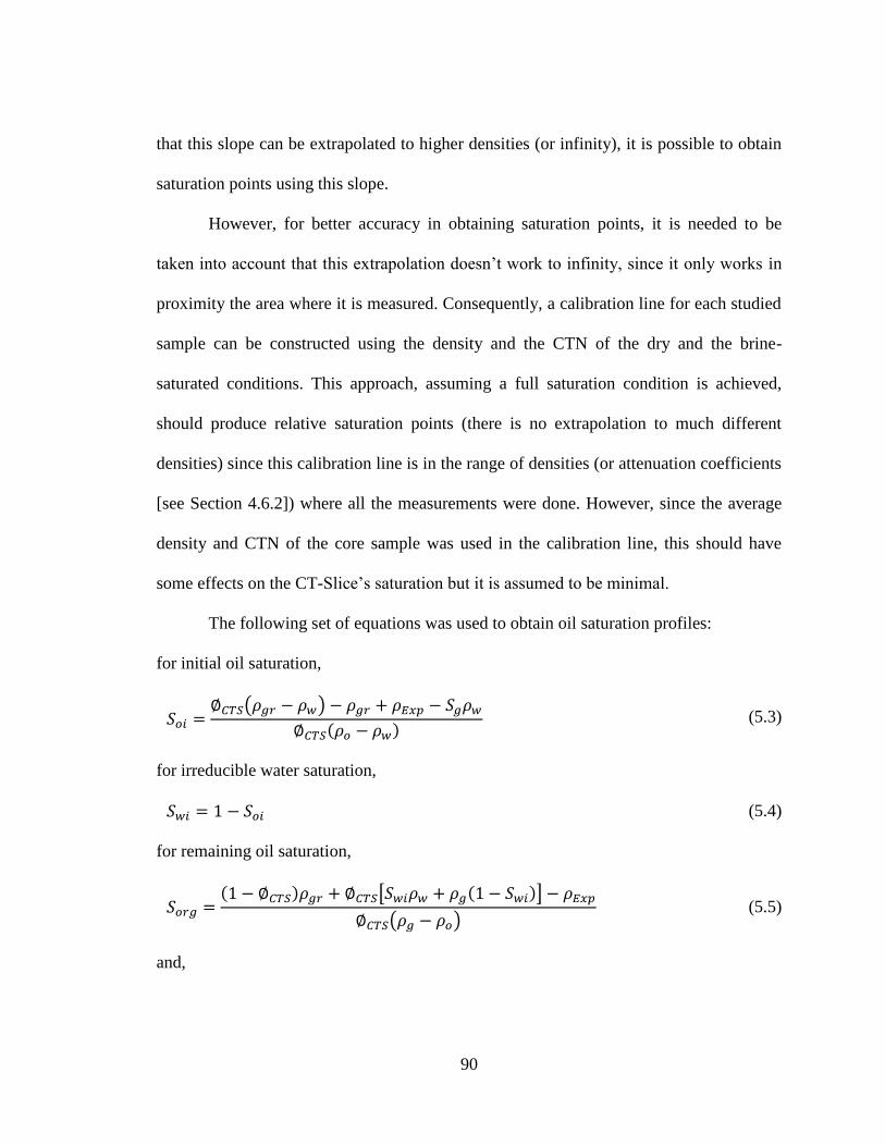
90
that this slope can be extrapolated to higher densities (or infinity), it is possible to obtain
saturation points using this slope.
However, for better accuracy in obtaining saturation points, it is needed to be
taken into account that this extrapolation doesn’t work to infinity, since it only works in
proximity the area where it is measured. Consequently, a calibration line for each studied
sample can be constructed using the density and the CTN of the dry and the brine-
saturated conditions. This approach, assuming a full saturation condition is achieved,
should produce relative saturation points (there is no extrapolation to much different
densities) since this calibration line is in the range of densities (or attenuation coefficients
[see Section 4.6.2]) where all the measurements were done. However, since the average
density and CTN of the core sample was used in the calibration line, this should have
some effects on the CT-Slice’s saturation but it is assumed to be minimal.
The following set of equations was used to obtain oil saturation profiles:
for initial oil saturation,
( )
(5.3)
for irreducible water saturation,
(5.4)
for remaining oil saturation,
[ ]
( ) (5.5)
and,

91
⟨ ⟩ ⟨ ⟩ ( ⟨ ⟩) (5.6)
where,
Grain density of the core sample (Kg/m3)
Brine density (Kg/m3)
Oil density (Kg/m3)
Gas density (Kg/m3)
Average porosity obtained for a CT scan slice (-)
Routine average porosity for a plug sample (-)
⟨ ⟩ Average CTN for a plug sample in dry condition (-)
⟨ ⟩ Average CTN for a plug sample saturated with brine (-)
Average CTN of a CT scan slice before or after gasflood (-)
It is to be noted that the saturation points obtained from CT scan are within a limit
of accuracy. This limit of accuracy was obtained by comparing the average saturation for
the core stack obtained from CT scan with that measured from material balance. The
limits of accuracy will be reported in this thesis whenever the saturation points obtained
from CT scan are presented.

92
Chapter Six: Experimental Results and Discussions
6.1 Properties of the Fluids Used in This Study
The recombined live-oil (used in the high pore-pressure (HPP) study) and the
produced crude oil (used in the low pore-pressure (LPP) study) were provided by Saudi
Aramco. These oils were obtained from Shaybah field in the Empty Quarter of Saudi
Arabia. The properties of both oils are presented in Table 6.1.
The brine used in both studies is synthetic brine, which was prepared using the
composition listed in Table 6.2. The properties of this brine are presented in Table 6.1.
The gas used in both studies is humidified nitrogen. The properties of the
humidified nitrogen in both tests’ conditions are also listed in Table 6.1.
Table 6.3 presents the results from interfacial tension measurements and
measurements conditions using the Pendant Drop Method. These measurements include
the interfacial tension between humidified N2 and brine, humidified N2 and crude oil, and
brine and crude oil. All interfacial tension measurements were carried out at an
international service lab (Intertek, USA).
The spreading coefficient (Table 6.3) was calculated using the results from Table
6.3 and Equation (3.3). The positive value of the spreading coefficient indicates that the
oil can spread on the brine in presence of the gas, which could promote oil film-flow.

93
Table 6.1: Properties of the fluids used in this study
Table 6.2: Synthetic brine composition
Table 6.3: Spreading coefficient for Oil, Water, and N2 fluid triplets
6.2 Rock Heterogeneity Effect on Oil Recovery from Centrifuge
This experimental study involve conducting single-speed drainage centrifuge runs
on nine core plugs selected from different rock heterogeneity as shown in Figure 6.1. The
main goal of this study was to evaluate the effect of rock heterogeneity on oil recovery
when gravity forces dominate the flow.

94
These drainage experiments were carried out at 80oC and 4000 RPM. It is
assumed that by operating at this speed, the capillary end-effect will be reduced. This
means that the controlling factor to oil recovery should be the rock heterogeneity.
Initially, these samples were saturated with oil at irreducible water saturation using a
centrifuge-speed of 6000 RPM (assuming connate water saturation is achieved at this
speed).
Table 6.4 presents the final results from this experimental part. Oil recovery factor
(Figure 6.2) showed a decreasing trend with initial oil saturation. Figure 6.3 shows that
irreducible water saturation is, in general, tied to the rock heterogeneity. Since pore-size
distribution and pore geometry are considered controlling factors of irreducible
saturation, the heterogeneity index adopted in this study could be a good indicator for the
irreducible water saturation in these rocks.
Figure 6.4 and Figure 6.5 illustrate the effect of rock heterogeneity on oil
recovery and Sorg, respectively. Generally, the MRH samples showed the highest oil
recovery whereas the HRH samples showed the lowest oil recovery. Moreover, the HRH
samples showed the highest Sorg values whereas the MRH samples showed the lowest Sorg
values. This shows that the rock heterogeneity affects the oil recovery and Sorg; however
the effect is not considered remarkable. This suggests that in the absence of the capillary
number recovery bases, the rock heterogeneity of those rocks has a minimal effect on oil
recovery.
One point worth mentioning is the close agreement in terms of oil recovery and
Sorg between sample 6 (from MRH group) and sample 8 (from other1 group). The
respective locations of these samples on the rock heterogeneity characterization map are

95
shown in Figure 6.1. This map shows that the respective locations of these two samples
are relatively close, although they were classified into different groups. This suggests that
sample six should not be included in the MRH group. This indicates that there might be a
heterogeneity index cut-off that marks the contribution of samples to oil recovery.
However, more centrifuge data are needed to reach to a consolidated conclusion
regarding this observation.
Overall, there is a general increasing trend in oil recovery and decreasing trend in
Sorg with irreducible water saturation. This supports what has been reported in the
literature concerning the relationship between oil recovery (and Sorg) and irreducible
water saturation.
Table 6.4: Results from single-speed drainage centrifuge experiments

96
Figure 6.1: Respective locations of the samples used in the centrifuge study
Figure 6.2: Oil recovery factor versus initial oil saturation from centrifuge
S1
S2 S3 S4
S5 S6
S7 S9
S8

97
Figure 6.3: Relation between heterogeneity type and irreducible water from
centrifuge study
Figure 6.4: Relation between heterogeneity type and total oil recovery from
centrifuge study

98
Figure 6.5: Relation between heterogeneity type and remaining oil saturation from
centrifuge study
6.3 Rock Heterogeneity Effect on Oil Recovery from Corefloods
The coreflood experiments conducted in this study are divided into two
experimental sets based on testing conditions: HPP conditions (17237 kPa and 80oC) and
LPP conditions (1034 kPa and 80oC). The main goal of conducting these experiments
was to evaluate the effect of rock heterogeneity on the ultimate oil recovery to immiscible
N2 gas injection under secondary and tertiary modes. In addition, a comparison can be
made between the two experimental sets to evaluate the effect of injection scheme
(constant injection pressure and constant injection rate) on oil recovery from different
rock heterogeneities. Since all runs from each experimental set were conducted under the
same experimental conditions, the outcomes from the two experimental sets can be
reasonably compared.

99
The LPP’s gasfloods consist of six runs. These runs were conducted on core
stacks from restored-wettability core plugs to evaluate the effect of a single rock
heterogeneity (four runs), and mixed rock heterogeneity (one run) on oil recovery factor.
All of the runs, performed as a secondary recovery process, were started with an initial
injection rate (IIR) that is equal to the critical gas injection (CIR) (Dumore, 1964) rate
multiplied by a factor of 7.3 except the MRH case (a factor of 4 was used).
(6.1)
where,
Density difference between oil and gas (kg/m3)
Viscosity difference between oil and gas (Pa.s)
Gravity acceleration constant (~8.31 m/s2)
Oil permeability at irreducible water saturation (m2)
Since conducting gravity stable gasfloods on these low permeability cores
requires a long period of time, it was decided to operate above the gravity stable injection
rates of those cores. Moreover, the 7.3 factor was chosen so that the LRH case can be
conducted at 0.008 (cm3/min) rather than (0.001) cm
3/min, which was the limit of the
used pump’s accuracy. Since the MRH showed the highest end point oil permeability
(9.19 mD), a factor of four was used instead of 7.3. This was a precautious step in order
to prevent early gas breakthrough in this run.
Two additional rates (10×IIR and 100×IIR) were used in most of those runs to
investigate whether the extra oil production is attributed to rock heterogeneity or capillary
end-effect phenomena. However, only two injection rates were used in the high rock

100
heterogeneity case because the CT scanner was not functioning during the scheduled
scanning period.
In order to evaluate the effect of rock heterogeneity type on the ultimate oil
recovery from immiscible gas N2 injection under tertiary recovery mode (initially flooded
with brine), one run was carried out on a core stack of mixed rock heterogeneity. This run
was conducted using single rate (4×CIR).
In addition to the LPP’s gasfloods, three runs were conducted at HPP (17237
kPa). These three runs evaluate the effect of a single rock heterogeneity type on oil
recovery (low, moderate and high rock heterogeneities). The tests were carried out on
core stacks from wettability-preserved core plugs.
6.3.1 Experimental Runs Performed at LPP
A total of six experimental runs were completed in this experimental part
evaluating the effect of rock heterogeneity type on oil recovery. Three runs evaluate the
effect of single rock heterogeneity on oil recovery from low rock heterogeneity (LRH),
moderate rock heterogeneity (MRH), and high rock heterogeneity (HRH). One run
compares the effect of the average rock permeability differences on oil recovery within
single rock heterogeneity (LRH). Another run evaluates the effect of mixed rock
heterogeneity (LRH, MRH, and Other1) on oil recovery. All of the previous experimental
runs were conducted in secondary recovery mode. The last experimental run evaluates
the effect of mixed rock heterogeneity (LRH, MRH, HRH, and Other1) on tertiary oil
recovery.

101
CT scanning was used in most of these runs to profile the fluid saturations at the
end of each injection rate period. In all of the multi-rate gasfloods, the starting time for
the next flow rate was when the ultimate oil recovery was achieved in the previous rate.
6.3.1.1 Effect of Single Rock Heterogeneity on Oil Recovery
The three gasfloods were conducted to evaluate the effect of single rock
heterogeneity on oil recovery from immiscible N2 gas injection as a secondary recovery
process. Table 6.5 and Table 6.6 present the results from the gasfloods and the individual
basic properties of the selected samples, respectively. Figure 6.6 through Figure 6.8
illustrate the respective locations of the selected samples from each run on the
heterogeneity characterization map. Figure 6.9 through Figure 6.14 summarize the data
obtained from these single rock heterogeneity gasfloods.
Each run has two sets of data that show the results from the first gas injection rate
(first set), and the multi-injection rates (second set). Part (a) in these sets provides the
data for oil recovery and the pressure drop when N2 gas was injected at connate water
saturation. Part (b) provides the data for oil and gas recoveries as a result of N2 gas
injection. Part (c) shows oil rate (OR) recovery when N2 gas was injected. Part (d)
illustrates the normalized recovery factor (NRF) described as (cumulative oil recovery
(fraction)/PV of N2 gas injected).

102
Table 6.5: Gasflood results from the LPP of the single heterogeneity rocks

103
Table 6.6: Basic properties of the core sample used to construct the single
heterogeneity stacks

104
Figure 6.6: Respective locations of the samples used to construct the LRH stack
Figure 6.7: Respective locations of the samples used to construct the MRH stack

105
Figure 6.8: Respective locations of the samples used to construct the HRH stack

106
(a) Oil recovery and pressure drop
characteristics
(b) Oil recovery and cumulative gas
produced characteristics
(c) Oil production rate characteristic (d) NRF characteristics
Figure 6.9: LRH gasflood results from the LPP for the first gas injection period

107
(a) Oil recovery and pressure drop
characteristics
(b) Oil recovery and cumulative gas
produced characteristics
(c) Oil production rate characteristic (d) NRF characteristics
Figure 6.10: LRH gasflood results from the LPP for the three gas injection periods

108
(a) Oil recovery and pressure drop
characteristics
(b) Oil recovery and cumulative gas
produced characteristics
(c) Oil production rate characteristic (d) NRF characteristics
Figure 6.11: MRH gasflood results from the LPP for the first gas injection period

109
(a) Oil recovery and pressure drop
characteristics
(b) Oil recovery and cumulative gas
produced characteristics
(c) Oil production rate characteristic (d) NRF characteristics
Figure 6.12: MRH gasflood results from the LPP for the three gas injection periods

110
(a) Oil recovery and pressure drop
characteristics
(b) Oil recovery and cumulative gas
produced characteristics
(c) Oil production rate characteristic (d) NRF characteristics
Figure 6.13: HRH gasflood results from the LPP for the first gas injection period

111
(a) Oil recovery and pressure drop
characteristics
(b) Oil recovery and cumulative gas
produced characteristics
(c) Oil production rate characteristic (d) NRF characteristics
Figure 6.14: HRH gasflood results from the LPP for the two gas injection periods

112
6.3.1.1.1 Comparison of the Three Single Heterogeneity Gasfloods
There are two major comparisons that can be made from the single heterogeneity
experiments completed: (i) effect of heterogeneity type on the secondary oil recovery,
and (ii) effect of heterogeneity type on the capillary end-effect. The effect of
heterogeneity type on the pressure drop and NRF characteristics will be discussed under
the first comparison. This sub-sections details this comparison for the single
heterogeneity gasfloods.
6.3.1.1.1.1 Effect of Single Rock Heterogeneity on Secondary Oil Recovery
Before discussing the results from the three single heterogeneity gasfloods, it is
more convenient to summarize the heterogeneity characteristics of these core stacks.
The LRH core stack showed generally similar porosity and NMR T2 distributions
which indicate overall uniformity in its rock property, as can be seen in Figure C. 25
through Figure C. 30. Furthermore, the pore size distribution from mercury injection of
this type of rocks showed generally uniform distributions (Figure A. 6 and Figure A. 7),
almost similar to the NMR T2 distributions. In this core stack, the air permeability
showed a standard deviation (STD) of 2.4 mD and an average permeability of 8.2 mD,
indicating fewer variations in permeability between core plugs and, in general, a tight
rock type.
On the other hand, the MRH core stack’s samples were marked with NMR T2
distributions that displayed small pores distribution (less than 100 ms) and a large pores
distribution (larger than 100 ms), as can be seen from Figure C. 11 through Figure C. 16.
Furthermore, the porosity distributions in these samples showed a generally similar
distribution to the NMR T2 corresponding to the large pores, with short skewedness

113
towards the smallest porosities that most probably corresponds to the small pores of the
NMR T2 distribution. The pore size distribution from mercury injection showed a bio-
model distribution (Figure A. 1 and Figure A. 2), and similar characteristics to the NMR
T2 distribution in these cores. In this core stack, the air permeability showed a STD of
13.6 mD and an average permeability of 29.2 mD, indicating more variations in
permeability (between the core samples) than the LRH and in general a permeable rock
type.
The HRH core stack’s samples showed in general wider NMR T2 distributions
suggesting broader pore size distributions as can be seen from the mercury injection data
(Figure A. 3). Similarly, these samples showed wider porosity distributions with some
samples illustrating bio-model porosity distributions (Figure C. 1 through Figure C. 5).
Commonly, this bio-model porosity distribution corresponds to a long skewedness
towards the short times of the corresponding NMR T2 distribution. In this core stack, the
air permeability showed a STD of 9.1 mD and an average permeability of 16.4 mD,
indicating more variations in permeability (between the core samples) than the LRH, but
less than the MRH.
The effect of single rock heterogeneity on oil recovery as a result from the first
injection rate is illustrated in Figure 6.15. This figure shows that there is a monotonic
trend in the total oil recovery factor with the rock heterogeneity though the MRH’s total
oil recovery with respect to that of the LRH and the HRH might be underestimated (to a
small extent). This is because the MRH run was conducted at (4×CIR) as mentioned in
Section 6.3.

114
Figure 6.16 shows that oil recovery from the LRH case (41.73% OOIP) is
significantly higher than the HRH case (21.34 % OOIP), even under the low pressure
immiscible mode of gas injection. These oil recovery numbers suggest that the
permeability variation within the cores is more important than the average permeability
of the core alone. For example, the LRH had the lowest oil permeability and yet showed
the highest oil recovery as compared to the HRH or the MRH, assuming the oil recovery
from the MRH was underestimated. These results also suggest that when immiscibly
operating on these types of rocks and with the aid of gravity, the highest oil recovery
would be expected from the LRH rocks more than what would be expected from the
other two heterogeneity rock types.
However, the centrifuge data suggests that when utilizing gravity forces, the
MRH rocks would show the highest oil recovery. This comparison between the two data
sets could indicate that the MRH rock likely has a better pore connectivity than the LRH
and HRH cases. Actually, by viewing the oil recovery curve from the MRH, it can be
seen that oil production almost immediately seized after gas breakthrough, while it is
obvious in the LRH and HRH cases that oil production continued in an incremental way
until the end of production. The poor recovery in the MRH is attributed to the complex
pore structure in these samples (suggesting oil trapping) as indicated from the
petrographic study conducted on the adjacent plugs of two samples from this group.
The incremental post-breakthrough recovery in the LRH case is assumed to result
from non-uniform displacement since the test was conducted using gas injection rate of
7.3×CIR. Although the samples of the LRH core stack are classified as LRH rocks, their
heterogeneity varies within the range of the LRH. This, in fact, can be seen from the

115
results from NMR T2 and CT scan (e.g. Figure C. 26 and Figure C. 30). These figures
demonstrate that the samples displayed inclusions from continuous rock’s density type
(higher density indicates low porosity) throughout the length of the core plug. This could
actually cause a non-uniform gas flow which is expected to be the reason behind this
incremental behaviour in the oil recovery from this type of rock. This is even more
obvious in the HRH case, in which NMR T2 and CT scan data (e.g. Figure C. 1 and
Figure C. 5) suggest a non-uniform displacement. Moreover, the results from thin section
indicated that the HRH rocks showed different pore sizes that are well interconnected,
suggesting that oil could be displaced from both pore types to some extent, depending on
where oil resides. However, it is expected that oil residing in the large pores will be
displaced before oil in the small pores, which indicates an incremental post-breakthrough
recovery from this type of rock as well.
Figure 6.15 and Figure 6.16 show that the LRH has the latest gas breakthrough
(0.42 PV) and the highest post-breakthrough recovery (9.89% OOIP). The utilization
factors (Figure 6.17) pertaining to the LRH case showed high NRF values, until about 0.6
PV of gas were injected, followed by a non-exponential decline, suggesting sustained
higher gas utilization factors for the LRH rocks.
This is also suggested from the pressure drop in the LRH case, as compared to the
MRH and HRH (Figure 6.18), indicating high oil mobility in the LRH, and thus higher
oil recovery.

116
Figure 6.15: Oil recovery characteristics of the three single heterogeneity rocks for
the first gas injection period
(a) Gas breakthrough (b) Oil recovery at breakthrough
Figure 6.16: Results comparisons between the three single heterogeneity rocks
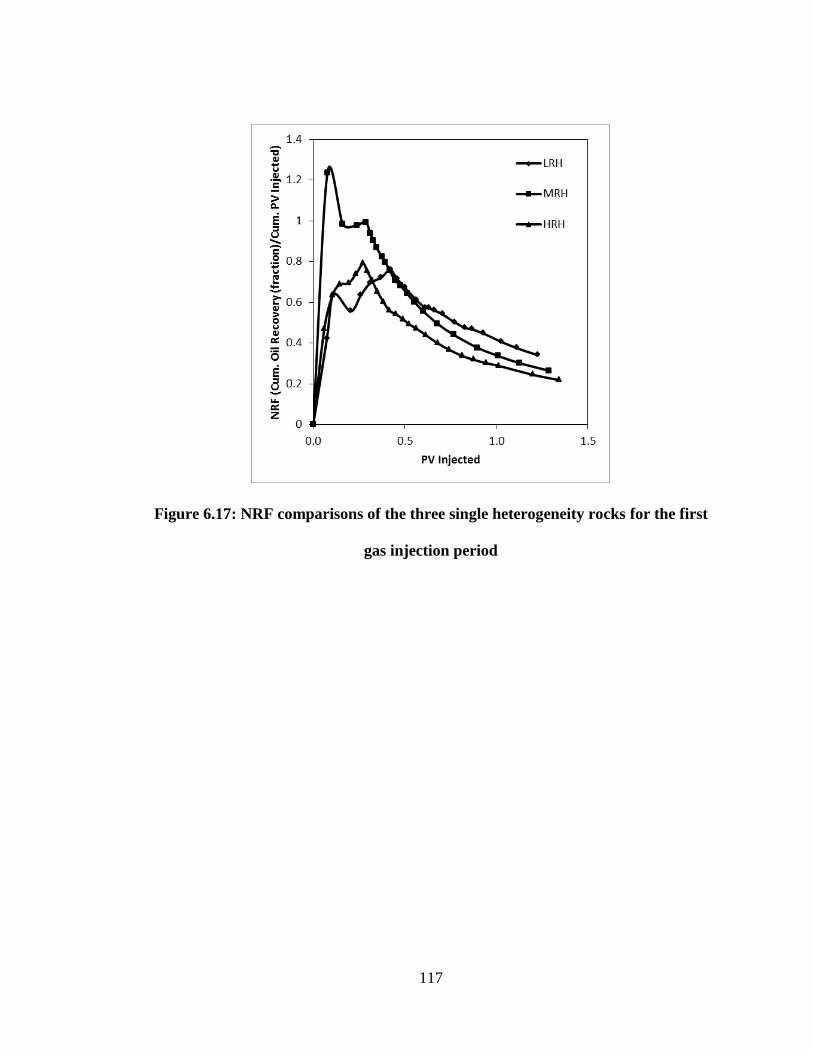
117
Figure 6.17: NRF comparisons of the three single heterogeneity rocks for the first
gas injection period

118
Figure 6.18: Pressure drop comparisons of the three single heterogeneity rocks for
the first gas injection period
6.3.1.1.1.2 Effect of Core Heterogeneity and Capillary End-Effect on Oil Recovery
Two factors affect oil recovery from laboratory immiscible gas displacements,
and that are rock heterogeneity (e.g. complex pore geometry or fracture), and capillary
end-effect. The first factor is caused by the nature of the rock while the second factor is
caused by the length of the rock. The core heterogeneity results in, for example, trapped
or bypassed oil. Oil trapping is usually caused by the pore geometry and the ratio of the
pore’s diameter to the throat’s diameter. The bypassed oil could result from the presence
of high permeability sections in the core such as fractured or dissolution channels. In this
case oil resides in fractures or dissolution channels will be displaced while the oil resides
in the matrix will be bypassed.

119
The capillary end-effect results from the wettability discontinuity of the wetting
phase (e.g. oil, as oil is being displaced by gas), which exist at the end of the core. In the
case of core stack, there is in fact a capillary end-effect at the interface of both cores.
However, this end-effect is small (capillary continuity is enforced by using filter paper
between core plugs, for example) as compared to the one at the end of the core stack.
This section investigates the role of core heterogeneity on capillary end-effect. The
magnitude of capillary end-effect in these core-stacks is also emphasised.
Figure 6.19 through Figure 6.21 illustrate oil saturation profiles for initial
saturation condition (Soi), remaining oil saturation from first gasflood (Sorg-1), remaining
oil saturation from second gasflood (Sorg-2), and remaining oil saturation from third
gasflood (Sorg-3). It can be seen from these figures that there is a saturation gradient as a
result of capillary end-effect even in the initial oil saturation. However, this saturation
gradient decreases (mostly at the bottom of the core-stack) as the gas injection rate
increases (increase in capillary number NC). The decrease in saturation gradient (mostly
at the bottom of the core-stack) is attributed mainly to capillary end-effect while the
decrease in the upper parts of the core-stack is assumed to be due to rock heterogeneity.
The upper part of the LRH core-stack, that is assumed to be less affected by the
capillary end-effect, is within this core’s depth interval (-153 – 0 mm). It can be seen in
Figure 6.19 that the LRH rocks showed a uniform change in the oil saturation between
the first two injection rates (flood accessed the non-swept areas from the core-stack). This
illustrates that the rock heterogeneity in these cores are almost identical, suggesting
similar results from increasing the NC. However, this was not the case for sample 4 (-153

120
to -108 mm) in this core stack, where it showed an increase in oil saturation from the
second NC as compared to the first NC. This could be a result from poor core-core
capillary contact (Figure 6.19).
Figure 6.10 shows that at the start of the second injection rate the pressure drop
displayed a sharp increase. This could result from fluids’ redistribution inside the core-
stack since CT scanning (about three hours CT scanning time) was performed between
the injection rates’ periods. The results (Figure 6.19) from further increasing the injection
rate (third NC) were significant in the bottom of the core stack and in the fourth sample
(reducing capillary end-effect and accessing new areas of the core-stack).
The MRH case showed some interesting observations (Figure 6.20) for the upper
part of the core stack (-188 to 0 mm). It shows that, for the core samples in this stack (-
141 to 0 mm), the oil incremental recovery from the second NC was very low, when
compared to the first NC. This observation reinforces the previous assumption that the
total oil recovery from the MRH was underestimated (to a small extent), as a result of
operating at (4×CIR).
On the other hand, sample five in this core stack (-188 to -143 mm) showed
different behaviour (fair amount of oil produced at the second NC) as compared to the
first 4 core plugs. This is assumed to be a result of capillary end-effect and rock
heterogeneity. The fact that this sample is closely located near the end of this core stack
made it possible to be affected by the capillary end-effect only to some extent. The effect
from the rock heterogeneity is assumed to be related to the broadest NMR T2 distribution
this sample exhibited (Figure 6.22) as compared to the other samples in this core stack.

121
The pressure response (Figure 6.12) pertaining to the second injection rate
maintained higher pressure values as a result of reducing the trapped oil in this core-stack
(mainly from the fifth core plug ). The pressure drop response (Figure 6.12) pertaining to
the third gas injection rate showed a fast pressure decrease after reaching a pressure peak
(~ 4 PV) suggesting less incremental oil recovery (less amount of oil, that was held by
capillary end-effect and was trapped by rock’s heterogeneity, was produced). This
pressure drop also showed a pressure peak at about 5 PV, which resulted from fluids’
redistribution inside the core-stack (probably connate water).
In the HRH case, only two injection rates were used. The results from oil
saturation profiles (Figure 6.21) showed that all of the samples in this stack have a similar
rock heterogeneity effect on the incremental oil recovery. This can be seen from the fact
that the oil saturation profile from the second NC showed very similar saturation profile
characteristics to the first NC. This shows that the variation in the average permeability
between the core plugs has minimal effect on the incremental oil recovery for each
sample, whereas the variation of permeability-and-porosity within these samples is more
important. The pressure drop (Figure 6.14) pertaining to the second injection rate
maintained higher pressure values until about 4 PVs of gas were injected suggesting
access of the flood to the non-swept areas of the core-stack.
By comparing these results from the three runs, it can be seen that the change in
oil saturation in the LRH case as a result of increasing NC by a factor of 10 suggest a fair
incremental amount of oil. The MRH, on the other hand, suggested the need of higher NC
in order to produce a fair incremental amount of oil. This is a result from comparing a
complex pore structure to a uniform pore structure as suggested by the thin-section study.

122
Unfortunately, it is not possible to compare the HRH case to the LRH and MRH cases (to
evaluate the effect of NC magnitude on increment oil recovery), since there is no data
available (from the second NC) for the HRH case. In general, the results from these
experimental runs suggest that the HRH rock’s heterogeneity magnified the effect of
capillary end-effect in this core-stack as compared to the LRH and MRH cases
Figure 6.19: Oil saturation profiles (from CT scan) for the LRH rock (data
accuracy: Swi (±0.06%), Sorg1 (± 0.47%), Sorg2 (± 0.88%), and Sorg3 (±0.78%))

123
Figure 6.20: Oil saturation profiles (from CT scan) for the MRH rock (data
accuracy: Swi (±0.23%), Sorg1 (± 0.58%), Sorg2 (± 1.16%), and Sorg3 (±0.76%))

124
Figure 6.21: Oil saturation profiles (from CT scan) for the HRH rock (data
accuracy: Swi (±0.07%), Sorg1 (± 1.46%), and Sorg3 (±1.65%))

125
Figure 6.22: NMR T2 distributions of the samples used to construct the MRH stack

126
6.3.1.1.2 Effect of Mixed Rock Heterogeneity on Secondary Oil Recovery
This experimental run evaluates the effect of multi rock heterogeneities on oil
recovery from secondary gas injection mode. Figure 6.23 illustrates the respective
locations of selected samples on the heterogeneity characterization map. The basic
properties of these samples are presented in Table 6.7. Cores from the HRH were
excluded from this run since they showed lower oil recovery when compared to the LRH
and MRH cases (as suggested by the single rock heterogeneity runs). Furthermore, from
the fact that the majority of the classified samples fall in the MRH category and that the
LRH run showed the highest total oil recovery, it was decided to construct this run based
on the MRH and the LRH samples. However, one sample from the Other1 group was
also included, since a sample (from centrifuge study) from this group had shown the
highest oil recovery (lowest Sorg), when compared to the other samples from the other
heterogeneity groups (Table 6.4). Sample 3 and 5, and sample six from this run were used
in the MRH and LRH single rock heterogeneity runs, respectively.
Table 6.8 presents the results from this experimental run. The results from this run
are presented in Figure 6.24 and Figure 6.25, similar presentation as the single rock
heterogeneity cases. Figure 6.26 shows that the total oil recovery from the MIRH
outperforms these from the single rock heterogeneities. The results from CT scan (Table
6.9) indicate that the highest oil recovery based on the individual core plug’s oil recovery,
came from the Other1’s sample (represents 16.1% of the total core stack’s PV). This is in
agreement with the results from centrifuge, suggesting that the oil production from this
sample was more attributed to gravity forces (the absolute air permeability of this sample
is 79.0 mD).

127
The MRH samples in the MIRH core stack showed moderate oil recoveries,
except one sample which showed a low oil recovery. This is because of the capillary end-
effect in this sample as shown in Figure 6.28 (-61 to -36 mm), probably because of poor
core-to-core capillary contact. Similarly, one sample from the two LRH samples in this
run showed a very low oil recovery as compared to its oil recovery from the single rock
heterogeneity run. This is also attributed to the capillary end-effect in this sample as a
result of poor core-to-core capillary contact as shown in Figure 6.28 (-150 to -100 mm).
The results from this run indicated that the LRH and MRH core plug’s individual
oil recoveries from the single and mixed rock heterogeneity cases are very similar. This
suggests that the additional oil recovery from the MIRH run, when compared to the LRH,
MRH, and HRH runs, can be more attributed to the first sample in the MIRH core stack
(sample1 from the Other1 group). This shows the advantage of having such a “good
quality” rock in a reservoir that is being immiscibly flooded with the aid of gravity
forces.
Figure 6.26 also illustrates that in general the oil recovery from the MIRH showed
similar behaviour as the LRH and MRH. On the other hand, it is interesting to observe
that the NRF for the MIRH core showed high NRF values till 0.6 PV injected (Figure
6.27), similar to the LRH core. The decline after that showed a non-exponential decrease
for a small PV injected (also similar to the LRH) followed by an exponential decrease,
which is similar to the MRH core. This suggests that the presence of the LRH rocks in a
reservoir will result in high gas utilization efficiencies. The pressure drop behaviour
(Figure 6.24(a)) tends to reach a plateau suggesting high sweep efficiency during this
gasflood.

128
Figure 6.23: Respective locations of the samples used to construct the MIRH stack
Table 6.7: Basic properties of the core samples used to construct the MIRH stack

129
Table 6.8: Gasflood results from the MIRH rocks
Table 6.9: Gasflood results for the individual MIRH samples from CT scan (data
accuracy: Swi (±0.18%), Sorg1 (± 0.92%), and Sorg3 (±1.31%))

130
(a) Oil recovery and pressure drop
characteristics
(b) Oil recovery and cumulative gas
produced characteristics
(c) Oil production rate characteristic (d) NRF characteristics
Figure 6.24: MIRH gasflood results from the LPP for the first gas injection period

131
(a) Oil recovery and pressure drop
characteristics
(b) Oil recovery and cumulative gas
produced characteristics
(c) Oil production rate characteristic (d) NRF characteristics
Figure 6.25: MIRH gasflood results from the LPP for the three gas injection periods

132
Figure 6.26: Oil recovery characteristic for the LRH, MRH, HRH, and MIRH rocks
Figure 6.27: NRF characteristic for the LRH, MRH, HRH, and MIRH rocks

133
Figure 6.28: Oil saturation profiles (from CT scan) for the MIRH rock (data
accuracy: Swi (±0.18%), Sorg1 (± 0.92%), and Sorg3 (±1.31%))
6.3.1.1.3 Effect of Average Core’s Permeability on Secondary Oil Recovery
It can be seen from the method followed in classifying heterogeneity that the
difference between average permeabilities within certain rock heterogeneity types was
overlooked since the purpose was to study the effect of variation in permeability and
porosity within a sample. This indicates that there exist within one single heterogeneity

134
group (e.g. LRH) low permeability LRH and high permeability LRH cores. Therefore, it
is of valuable information to study the effect of the average core’s permeability on oil
recovery. In this comparison, the difference in effective oil permeability is emphasized.
To achieve this objective, a core from the LRH samples was constructed (Table
6.10). Table 6.10 also presents the results from this experimental run. The respective
location of the selected sample on the heterogeneity characterization map is shown in
Figure 6.29. The results from this run are compared against the previous results from the
low LRH permeability (Figure 6.30). Though, the high permeability LRH core showed
higher oil recovery (46.96% OOIP) as compared to the low permeability LRH core stack
(41.94% OOIP), the effect of the average core permeability on oil recovery is minimal
(Figure 6.30(a)). An additional reason that is believed to contribute to the difference in oil
recovery is that the high permeability core showed higher variation in permeability
(higher STD_T2FF) than most of the samples used to construct the low permeability core
stack.
Moreover, both cases showed almost similar NRF characteristics (Figure 6.30(b)),
except that the low permeability LRH case showed a non-exponential declining trend
suggesting higher gas utilization efficiencies as compared to the high permeability case.
The pressure drop behaviour (Figure 6.30(c)) suggests that the low permeability core
showed lower gas mobility as compared to the high permeability core, indicating possible
incremental oil recovery had the low permeability core been flooded for extra PVs.

135
Table 6.10: Gasflood results from the LPP of the high permeability LRH rock
Figure 6.29: Respective location of the high permeability LRH sample

136
(a) Oil recovery characteristics (b) NRF characteristics
(c) Pressure drop characteristics
Figure 6.30: Comparison between the LPP’s gasflood results from the low and high
permeability LRH rocks

137
6.3.1.1.4 Effect of Mixed Rock Heterogeneity on Tertiary Oil Recovery
This experimental run evaluates the effect of multi rock heterogeneities on oil
recovery from tertiary gas injection mode. The current production practice employed on
the reservoir under study (the cores under study represent a main formation in this
reservoir) has been gas cap expansion (pressure maintenance). However, in the case this
type of rock is produced by waterflooding, it is possible to employ gas injection in
tertiary recovery mode, since the immiscible gas injection for commercial purposes has
been employed in both secondary as well as tertiary modes.
Figure 6.31 illustrates the respective locations of the selected samples on the
heterogeneity characterization map. Table 6.11 and Table 6.12 present the results from
the water-and gasfloods and the individual basic properties of the selected samples,
respectively. Figure 6.32 summarizes the data obtained from the waterflood.
Part (a) provides the data for oil recovery and pressure drop when water was
injected at connate water saturation. Part (b) provides the data for oil and water
recoveries as a result of water injection. Part (c) shows oil rate (OR) recovery when water
was injected.
Figure 6.32 (a), illustrates the significant performance from waterflooding this
type of rock, as suggested from the high total oil recovery achieved in this case (64.78 %
OOIP). The high pressure drop (Figure 6.32 (a)) suggests very high sweep efficiency
from waterflooding.
After reaching the ultimate oil recovery from waterflooding, the core was
positioned vertically and then N2 gas was introduced at a rate that is 1.7×CIR. The total

138
injection time was about 36 days (equivalent to 1.41 PVI). Figure 6.33 summarizes the
data obtained from the gasflood.
Part (a) of this figure provides the data for fluid recovery when gas was injected at
remaining oil saturation from waterflooding. Part (b) provides the data for oil and gas
recoveries as a result of gas injection. Part (c) shows the pressure drop characteristics
when gas was injected. Part (d) illustrates the normalized recovery factor (NRF)
described as (cumulative remaining oil recovery (fraction)/PV of N2 gas injected).
Figure 6.33(a) shows that gas breakthrough occurred at 0.28 PVI. It also can be
seen that oil started with a fast production (at about 0.26 PVI), and then maintained an
almost constant incremental production trend. This can be attributed to film flow
drainage since the spreading coefficient in this system is positive and the wettability is
intermediate. The results from the tertiary recovery mode showed excellent average
incremental recovery (~35.0% ROIP), even under the immiscible mode of injection.
Moreover, at the time of the experiment termination, oil production still showed an
incremental trend suggesting further oil recovery (Figure 6.33(b)).
The pressure behaviour (Figure 6.33(c)) showed a fast decrease after gas
breakthrough where it maintained a constant pressure drop at about 70 kPa starting from
about one PVI until the end of the experiment, suggesting that oil is being produced from
film drainage. The pressure drop behaviour in this tertiary mode almost showed similar
behaviour as the pressure drop in the secondary mode (e.g. MIRH). This similarity in the
pressure drop’s patterns suggests similar mechanistic and dynamic characteristics of these
core floods. The high pressure drop observed in the tertiary recovery mode gasflood, as

139
compared to that from the secondary mode, is assumed to be related to the relatively
higher water saturations in the upper-portion of the core during this experiment.
The NFR from the tertiary recovery mode (Figure 6.33(d)) showed low gas
utilization factors (low NFR values) as compared to the secondary recovery mode,
suggesting a lower gas utilization factor for the tertiary mode.
Figure 6.34 illustrates the results from CT scan during this experiment. It is
presented as on the basis of bulk density rather than oil saturation since obtaining
corresponding oil saturation values are challenging under the current experimental
conditions. In the case of waterflooding, the change (increase in density) of the line
designated with “waterflooded” towards the line designated with “brine saturated”
indicates reduction in oil saturation. The change (decrease in density) in the line
designated with “gasflooded” away from the “brine saturated” line indicates reduction in
liquid saturation.
This figure shows that in the case of waterflooding, all the core plugs showed
almost similar water sweep efficiency except one sample (Other1). On the other hand, in
the case of gasflood the change in the “gasflooded” line showed corresponding change
with the core’s heterogeneity. This suggests that oil recovery from immiscible gas
injection in these types of rocks is more sensitive to heterogeneity than oil recovery from
water injection.

140
Table 6.11: Basic properties of the core samples used to construct the MIRH stack
for tertiary gasflood
Table 6.12: Results from secondary (waterflood) and tertiary (gasflood) recovery for
the MIRH rocks

141
Figure 6.31: Respective locations of the samples used to construct the HIRH stack
for tertiary gasflood

142
(a) Oil recovery and pressure drop
characteristics
(b) Oil recovery and cumulative water
produced characteristics
(c) Oil production rate characteristic
Figure 6.32: Results from secondary recovery mode (waterflood)

143
(a) Fluid recovery characteristics (b) Oil and gas recovery characteristics
(c) Pressure drop characteristics (d) NRF characteristics
Figure 6.33: Results from tertiary recovery mode (gasflood)

144
Figure 6.34: Bulk density (from CT scan) profiles for secondary and tertiary
recovery modes for MIRH rocks
6.3.2 Experimental Runs Performed at HPP
A total of three experimental runs conducted under HPP conditions were
completed in this experimental part. The main objectives of conducting these experiments
were: (i) to evaluate the effect of rock heterogeneity (LRH, MRH, and HRH) on the

145
secondary oil recovery, and (ii) to evaluate the ultimate oil recovery from high pressure
injection mode.
It is to be noted that the production initiation in each run was done by decreasing
the BPR using small pressure steps until a continuous and smooth production was
achieved. This procedure seemed to work well for the LRH and HRH, but not very well
for the HRH, as will be shown in the following discussions.
Table 6.13 presents the results from the gasfloods and the core stack’s basic
properties, respectively. Figure 6.35 through Figure 6.37 summarize the data obtained
from these gasfloods.
Part (a) provides the data for oil recovery and pressure drop when N2 gas was
injected at connate water saturation. Part (b) provides the data for oil and gas recoveries
as a result of N2 gas injection. Part (c) shows oil rate (OR) recovery when N2 gas was
injected. Part (d) illustrates the normalized recovery factor (NRF) described as
(cumulative oil recovery (fraction)/PV of N2 gas injected).

146
Table 6.13: Results from the gasfloods performed at HPP for the single
heterogeneity rocks (LRH, MRH, and HRH)
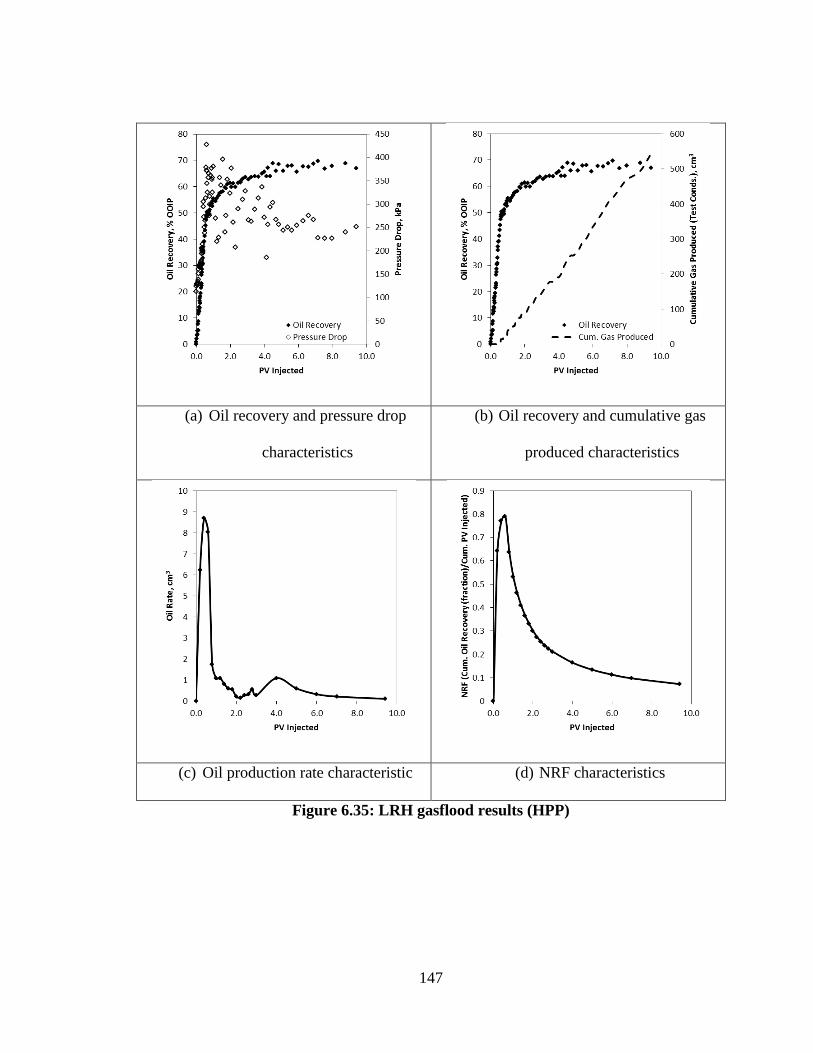
147
(a) Oil recovery and pressure drop
characteristics
(b) Oil recovery and cumulative gas
produced characteristics
(c) Oil production rate characteristic (d) NRF characteristics
Figure 6.35: LRH gasflood results (HPP)

148
(a) Oil recovery and pressure drop
characteristics
(b) Oil recovery and cumulative gas
produced characteristics
(c) Oil production rate characteristic (d) NRF characteristics
Figure 6.36: MRH gasflood results (HPP)

149
(a) Oil recovery and pressure drop
characteristics
(b) Oil recovery and cumulative gas
produced characteristics
(c) Oil production rate characteristic (d) NRF characteristics
Figure 6.37: HRH gasflood results (HPP)
The results from the three gasfloods are compared in Figure 6.38. The comparison
includes oil recovery, the pressure drop across the core, and NFR. Figure 6.38(a)
illustrates that the highest total oil recovery was from the LRH core, similar results to the

150
LPP’s gasfloods. However, this is not the case for the MRH and the HRH as they showed
identical total recoveries. This is apparently the result from operating at high pressure
drop in the case of HRH (Figure 6.38(b)), which was caused by the way that oil
production was initiated. Since the results from the LPP suggest that there is a virtual
difference in total oil recoveries between the MRH and the HRH, similar recovery’s trend
in the HPP runs was expected to be seen as well (performed at similar conditions).
However, operating at a high pressure drop minimised the effect of rock’s
heterogeneity in the HRH core leading to similar results as the MRH. This is also clear
from the fact that the MRH and HRH cores showed almost similar oil permeabilities
(12.86 mD, for the HRH versus 11.02 mD, for the MRH), and that the HRH had earlier
gas breakthrough (~ 0.01 PVI, for the HRH versus ~ 0.28 PVI, for the MRH).
Consequently, the only way to bring up the oil recovery for the HRH core is to operate at
high pressure drop. Thus, the total oil recovery from the HRH was overestimated as a
result of the experimental procedure and not the rock’s nature.
The utilization factor pertaining to the LRH case showed high NRF till 0.6 PVI
(similar result to the LRH from the LPP), followed by an exponential decline. However,
this decline was less severe as compared to the MRH case, suggesting higher gas
utilization factor, when compared to the MRH case.

151
(a) Oil recovery characteristics (b) Pressure drop characteristics
(c) NRF characteristics
Figure 6.38: Comparison between the three single heterogeneity rocks (HPP)

152
Chapter Seven: History Matching Study
7.1 Simulator Used in This Study
The Sendra simulator was used to conduct this history matching. Sendra is a
commercial lab simulator (developed for special core analysis), which is based on fully
implicit black oil formulation (for two-phase flow). Moreover, Sendra is not constrained
to the limiting assumptions, such as zero capillary pressure and homogenous core sample,
which are made by analytical method. Furthermore, it includes the necessary options for
laboratory applications (core geometry and physical properties are very easy to handle)
(SENDRA, 2013). This simulator matches the experimental data (e.g. oil production and
pressure drop) by varying the relative permeability and capillary pressure curves
(different relative permeability and capillary pressure models can be selected) until a
satisfactory match is achieved. This matching way corrects for the capillary end-effect,
which was obvious in the experimental results from this study, specifically the LPP’s
secondary gasfloods.
7.2 History Matching Experimental Results from Two Phase Flow
Only the experimental results from two-phase flow were history matched using
Sendra. These include all of the LPP and at HPP runs as well as the waterflood run.
However, only the production data (from the low pore-pressure) corresponding to the
first gas injection rate was matched. Corey relative permeability model and Skjaeveland
capillary pressure model were used for all of the history matching work completed.
Fluid properties (viscosity, density, and compressibility), core properties
(porosity, and absolute permeability or end point oil permeability), end point saturations
(connate water, initial oil, and residual oil saturations), and core’s dimensions (length and

153
diameter) were used as well as the coreflood data to perform history matching work using
Sendra. In this study, the Klinkenberg-absolute permeability was used as the base
permeability for all of the history matching work completed. In Sendra, gasflood data is
matched by fixing the relative permeability to gas (at residual oil saturation) and varying
the relative permeability to oil at connate water saturation. The relative permeability to
oil at connate water saturation was fixed in the case of history matching the waterflood
data. Since, the main objective of this history matching is to correct for capillary end-
effect, Sorg was not fixed during the history matching.
Figure 7.1 through Figure 7.5 shows the history matching results from the LPP
experiments, while Figure 7.6 through Figure 7.8 illustrate the history matching results
for the experiments performed at HPP. The results from history matching the waterflood
experiment are shown in Figure 7.9. These results show a satisfactory match between the
experimental data and the simulated data.

154
Figure 7.1: History matching results (LRH: LPP)
Figure 7.2: History matching results (MRH: LPP)

155
Figure 7.3: History matching results (HRH: LPP)
Figure 7.4: History matching results (MIRH: LPP)

156
Figure 7.5: History matching results (LRH-high perm.: LPP)
Figure 7.6: History matching results (LRH: HPP)

157
Figure 7.7: History matching results (MRH: HPP)
Figure 7.8: History matching results (HRH: HPP)

158
Figure 7.9: History matching results (MIRH-waterflood: LPP)
Table 7.1 and Table 7.2 compare the experimental results to the simulated results
from Sendra for the LPP and the HPP gasfloods, respectively. Figure 7.10 and Figure
7.11 compare the measured total oil recovery factor to the corrected total oil recovery
factor, for the LPP’s and HPP’s gasfloods, respectively. These figures show that the
difference between the original and the corrected oil recoveries is higher in the case of
the LPP’s gasfloods than the HPP’s gasfloods. This resulted from operating at lower NC
(in the LPP’s gasfloods) as compared to higher NC (in the HPP’s gasfloods).
Figure 7.12 plots the corrected oil recovery factors obtained from LPP and HPP
gasfloods versus the corresponding initial oil saturations. The corrected oil recovery
factors pertaining to the LPP gasfloods showed an increasing trend with the
corresponding oil saturations. The corrected oil recovery factors pertaining to the HPP

159
gasfloods showed a decreasing trend with the corresponding initial oil saturations. The
difference in irreducible water saturations between the two sets is postulated to be the
cause for this opposite trend illustrated in Figure 7.12.
The results from the LPP suggest that the rock heterogeneity (e.g. HRH)
magnified the effect of capillary end-effect. This is clear in the case of the HRH where it
showed before the correction the lowest oil recovery, whereas after the correction it
showed higher recovery than the MRH. Similarly, the HRH case from the HPP gasfloods
showed more total oil recovery than the MRH after capillary end-effect correction.
The results from this history matching study suggest that the heterogeneity type
(HRH) in these specific rocks could be not important, when compared to the MRH case
on the bases of “true” oil recovery. However, the results from the LPP (specifically oil
saturation profiles) indicated that the increase in NC produced less oil when compared to
the MRH and the LRH cases, suggesting a greater effect of heterogeneity on incremental
oil recovery. Moreover, the results from the centrifuge indicated lower total oil recovery
in the case of HRH.
The results from the above discussion could suggest that the correction for
capillary end-effect using Sendra was overestimated in the case of HRH. However, by
comparing the Sorg values from centrifuge to the corrected ones from gasfloods, it is clear
that the difference is minimal. Therefore, Sendra corrections were not overestimated.
Thus, a possible reason for this difference is the difference in the connate water
saturation. In general, these cores showed a decreasing trend in Sorg with increasing
connate water saturation.

160
Table 7.1: Comparison between measured and matched results (LPP’s gasfloods)
Table 7.2: Comparison between measured and matched results (HPP)
Figure 7.10: Comparison between measured and matched results (LPP’s gasfloods)

161
Figure 7.11: Comparison between measured and matched results (HPP)
Figure 7.12: Oil recovery factor versus initial oil saturation from all gasfloods

162
Chapter Eight: CONCLUSIONS AND RECOMMENDATIONS
8.1 Conclusions
Based on the characterization, experimental and history matching studies
completed in this research, the following conclusions were drawn:
1. Injecting water as a secondary recovery process resulted in higher oil
recovery (64.78% OOIP) than all secondary gasfloods. This leads to the
conclusion that waterflood could be a potential secondary recovery
process in this type of rocks, if it is economically feasible and
operationally applicable.
2. Injecting N2 gas in tertiary mode resulted in similar recovery to the MIRH
secondary mode (34.80% ROIP vs. 34.02% OOIP). However, if the
waterflood recovery (prior to N2) is considered, the ultimate recovery of
the tertiary mode is much higher at a later time. The combined recovery
from waterflood and gasflood (tertiary) is found to be 83.23% of OOIP.
3. The MIRH oil recovery (LRH, MRH, and Other1) showed outstanding
results (47.82% OOIP) as compared to the LRH, MRH, and HRH results
(41.94%, 34.02%, and 29.33% of OOIP, respectively). This is because the
MIRH core stack had a “good quality” rock sample (Other1) that showed
the highest oil recovery (~61% OOIP) as compared to the other samples
within the MIRH core stack (32.81%, 53.6%, 31.45%, 50.77%, and 32.4%
of OOIP).
4. Oil recovery from gas-oil displacement (LPP) using low pressure gradient
resulted in a monotonic trend with the rock heterogeneity. The LRH rocks

163
showed the highest oil recovery (41.94% OOIP) while the HRH rocks
showed the lowest oil recovery (29.33% OOIP). It is concluded that both
of the rock heterogeneity and the capillary end-effect caused this
monotonic trend. Moreover, capillary end-effects were significant under
the current operational conditions of these experiments.
5. The effect of different average rock permeabilities (2.67 mD versus 6.49
mD) from the same heterogeneity group (LRH) on oil recovery is minimal
(41.94% vs. 46.96% of OOIP). It is concluded that the difference in the
STD_T2FF (1.16 vs. 1.22) contributed to this difference in oil recovery,
since larger STD indicates broader pore-size distribution.
6. A new rock heterogeneity characterization map was developed. This
characterization approach is based on the variation of permeability and
porosity within an individual core sample. NMR T2 distributions were
used as the permeability variation indicator based on the close analogy to
pore size distribution, where this variation was estimated using the
STD_T2FF for each sample. CT scan was used to describe porosity
variations based on the direct relation to porosity, where this variation was
estimated using the CvCT. It was found that the selected samples can be
classified into three main heterogeneity groups, namely LRH, MRH, and
HRH. Based on the results from this characterization approach, a series of
gas-oil displacement experiments were conducted.

164
7. A new permeability predictor correlation was established (by linking the
K-C empirical correlation with the NMR total surface area of pores) and
verified using the selected samples.
8. Gas-oil displacement under favourable gravity drainage conditions
(centrifuge) resulted in oil recovery that is generally less sensitive to rock
heterogeneity of the cores under study.
9. More than 80 samples were selected and characterized for the effect of
rock heterogeneity on oil recovery from immiscible gas injection. This
characterization involved NMR, CT, wettability, mercury injection, and
petrographic studies. The results from these studies were implemented in
the discussion of gas-oil displacement experiments.
10. Correlating the absolute permeability of the selected cores to the T2
geometric mean of the free fluid portion of the total T2 spectrum showed
improved correlation as compared to the T2 geometric mean of the total T2
spectrum. This is because of the close relation between the average pore
size and the T2 geometric mean of the free fluid portion of the total T2
spectrum.
11. The results from the HPP’ runs showed almost similar oil recovery trend
with rock heterogeneity to that from the LPP gasfloods.
12. A lab simulator (corrects for capillary end-effect) was used to history
match all of the secondary gasflood results. The simulated results were
compared to the experimental values. Fair agreement was observed.

165
13. The true oil recoveries from the secondary gasfloods were estimated using
the results from history matching. It was found that the HRH rocks were
highly affected by capillary end-effect (more oil retained in the core) when
compared to the MRH rocks. The corrected oil recovery for the HRH
rocks was higher than the MRH rocks leading to the conclusion that the
heterogeneity type in these specific HRH rocks could be not important.
8.2 Recommendations
The following recommendations are offered for field applications:
1. This type of rock formation should always be produced separately, unless
operationally difficult. In addition, low production rates, if economically
feasible, should be implemented to take the advantage of gravity drainage
since gravity drainage is potentially a major recovery process in this
formation.
2. Waterflood, if it is operationally applicable and economically feasible,
could be implemented in this formation since it showed promising oil
recoveries.
The following recommendations are offered for future work on this subject:
1. A large selection of core samples from different rock formations showing
vugs, solution channels and fractures should be obtained. Following
which, NMR and CT measurements should be conducted for each sample.
After that, heterogeneity characterization maps can be constructed and
tested against each type of rock heterogeneity (e.g. samples showing dual
porosity and triple porosity), and mixed rock heterogeneity.

166
2. Gasflooding should be conducted using two types of rock heterogeneity in
order to study the effect of combined rock heterogeneity on oil recovery.
3. Two core stacks from each heterogeneity group having different average
permeability should be constructed to evaluate their effect on oil recovery.
4. Centrifuge experiments should be conducted on large set of samples from
different rock heterogeneities in order to build solid conclusions
concerning the effect of rock heterogeneity on oil recovery.
5. Long core stacks should be constructed in order to minimize the effect of
capillary end-effect in such tight rocks.
6. It is of valuable information to evaluate the magnitude effect of the
classified heterogeneities on oil recovery using miscible gas
(recommended gas CO2) injection under secondary and tertiary injection
modes.

167
References
Agbalaka, C., Dandekar, A., Patil, S., Khataniar, S., and Hemsath, J. (2008, October).
The Effect of Wettability on Oil Recovery: A Review. In SPE Asia Pacific Oil
and Gas Conference and Exhibition.
Ahr, W. M. (2000). Carbonate Pore Properties as Indices of Reservoir Quality. AAPG
Bulletin, 84(13).
Ahr, W. M., Allen, D., Boyd, A., Bachman, H. N., Smithson, T., Clerke, E. A., and
Ramamoorthy, R. (2005). Confronting the Carbonate Conundrum. Oilfield
Review, 17(1), 18-29.
Akin, S., and Kovscek, A. R. (2003). Computed Tomography in Petroleum Engineering
Research. Geological Society, London, Special Publications, 215(1), 23-38.
Al-Awami, F., Salamy, S., Hemanthkumar, K., and Sadler, R. (2005, November). A
Mega-Cell Simulation Model of Shaybah Field. In International Petroleum
Technology Conference.
Alfaraj, M., Nebrija, E. L., and Ferguson, M. D. (1998). The Challenge of Interpreting 3-
D Seismic in Shaybah Field. Saudi Arabia, GeoArabia, 3, 209-226.
Al-Ghamdi, N. M. (2006). Facies, Sequence Framework, and Evolution of Rudist
Buildups, Shu’aiba Formation, Saudi Arabia (Doctoral dissertation, Virginia
Polytechnic Institute and State University).
Ali, S. A., Clark, W. J., Moore, W. R., and Dribus, J. R. (2010). Diagenesis and Reservoir
Quality. Oilfield Review, 22(2).
168
Alsharhan, A. S. (1995). Facies Variation, Diagenesis, and Exploration Potential of the
Cretaceous Rudist-Bearing Carbonates of the Arabian Gulf. AAPG Bulletin-
American Association of Petroleum Geologists, 79(4), 531-550.
Alston, R. B., Kokolis, G. P., and James, C. F. (1985). CO2 minimum miscibility
pressure: A correlation for impure CO2 streams and live oil systems. Old SPE
Journal, 25(2), 268-274.
Al-Wahaibi, Y. M., Muggeridge, A. H., and Grattoni, C. A. (2009). Gas–oil non-
Equilibrium in Multicontact Miscible Displacements within Homogeneous Porous
Media. Journal of Petroleum Science and Engineering, 68(1), 71-80.
Amott, E. (1959). Observations Relating to the Wettability of Porous Media. Trans,
AIME, 216, 156-162.
Archie, G. E. (1950). Introduction to Petrophysics of Reservoir Rocks. AAPG Bulletin,
34(5), 943-961.
Bloembergen, N., Purcell, E. M., and Pound, R. V. (1948). Relaxation Effects in Nuclear
Magnetic Resonance Absorption. Physical Review, 73(7), 679.
Blunt, M., Zhou, D., and Fenwick, D. (1995). Three-Phase Flow and Gravity Drainage in
Porous Media. Transport in porous media, 20(1-2), 77-103.
BP. (2007). BP Statistical Review 2007 (accessed Jun 16, 2013): http://www.bp.com
Brock, D. C., and FM, O. (1991, October). Flow Visualization of Viscous Fingering in
Heterogeneous Porous Media. In SPE Annual Technical Conference and
Exhibition.

169
Brown, R. J. S., and Neuman, C. H. (1980). Processing and Display of Nuclear
Magnetism Logging Signals: Application to Residual Oil Determination. Trans.
SPWLA, 1-25.
Brown, R., and Fatt, I. (1956, October). Measurements of Fractional Wettability of Oil
Fields' Rocks by the Nuclear Magnetic Relaxation Method. In Fall Meeting of the
Petroleum Branch of AIME.
Burger, J., and Mohanty, K. (1997). Mass Transfer from Bypassed Zones During Gas
Injection. SPE Reservoir Engineering, 12(2), 124-130.
Butler, J. P., Reeds, J. A., and Dawson, S. V. (1981). Estimating Solutions of First Kind
Integral Equations with Nonnegative Constraints and Optimal Smoothing. SIAM
Journal on Numerical Analysis, 18(3), 381-397.
Coats, K. H., and Smith, B. D. (1964). Dead-End Pore Volume and Dispersion in Porous
Media. Old SPE Journal, 4(1), 73-84.
Catalan, L., Dullien, F., and Chatzis, I. (1994). The Effects of Wettability and
Heterogeneities on the Recovery of Waterflood Residual Oil with Low Pressure
Inert Gas Injection Assisted by Gravity Drainage. SPE Advanced Technology
Series, 2(2), 140-149.
Chatzis, I., and Ayatollahi, S. (1993). The Effect of Gas Injection Rate on the Recovery
of Waterflood Residual Oil under Gravity Assisted Inert Gas Injection. In
Technical Meeting/Petroleum Conference Of The South Saskatchewan Section.
Chatzis, I., Kantzas, A., and Dullien, F. A. L. (1988, October). On the Investigation of
Gravity-Assisted Inert Gas Injection using Micromodels, Long Berea Sandstone

170
Cores, and Computer-Assisted Tomography. In SPE Annual Technical
Conference and Exhibition.
Chatzis, I., Morrow, N., and Lim, H. (1983). Magnitude and Detailed Structure of
Residual Oil Saturation. Old SPE Journal, 23(2), 311-326.
Choquette, P. W., and Pray, L. C. (1970). Geologic Nomenclature and Classification of
Porosity in Sedimentary Carbonates. AAPG bulletin, 54(2), 207-244.
Cordesman, A. H., and Obaid, N. E. (2005). National Security in Saudi Arabia: Threats,
Responses, and Challenges. Greenwood Publishing Group.
Corey, A. T. (1954). The Interrelation between Gas and Oil Relative Permeabilities.
Producers monthly, 19(1), 38-41.
Cueic, L.E. (1991). Evaluation of Reservoir Wettability and its Effect on Oil Recovery.
Interfacial Phenomena in Petroleum Recovery, 36, 319.
Danesh, A. (1998). PVT and Phase Behaviour of Petroleum Reservoir Fluids (Vol. 47).
Elsevier.
Dezabala, E., and Kamath, J. (1995, October). Laboratory Evaluation of Waterflood
Behavior of Vugular Carbonates. In SPE Annual Technical Conference and
Exhibition.
Donaldson, E., Thomas, R., and Lorenz, P. (1969). Wettability Determination and its
Effect on Recovery Efficiency. Old SPE Journal, 9(1), 13-20.
Dumore, J. M. (1964). Stability Considerations in Downward Miscible Displacements.
Old SPE Journal, 4(4), 356-362.
Dumore, J. M., and Schols, R. S. (1974). Drainage Capillary-Pressure Functions and the
Influence of Connate Water. Old SPE Journal, 14(5), 437-444.

171
Dunham, R. J. (1962). Classification of Carbonate Rocks According to Depositional
Texture.
Dykstra, H., and Parsons, R. L. (1950). The Prediction of Oil recovery by Waterflood.
Secondary Recovery of Oil in the United States, 2, 160-174.
Egermann, P., Robin, M., Lombard, J. M., Modavi, A., and Kalam, M. Z. (2003). Gas
Process Displacement Efficiency Comparisons on a Carbonate Reservoir. Middle
East Oil Show.
Gates, I. D. (2011). Basic Reservoir Engineering. Kendall-Hunt Inc.
Gaucher, D. H., and Lindley, D. C. (1960). Waterflood Performance in a Stratified Five
Spot Reservoir, A Scaled Model Study. Trans. Am. Inst. Min. Metall. Pet. Eng,
219, 208-215.
Hagoort, J. (1980). Oil Recovery by Gravity Drainage. Old SPE Journal, 20(3), 139-150.
Horbury A.D., and Simmons, M.D. (2001). Arabian Plate Sequence Stratigraphy.
Hughes, G. W. (2000). Bioecostratigraphy of the Shu'aiba Formation, Shaybah field,
Saudi Arabia. GeoArabia-Manama, 5, 545-578.
Jensen, J. L., Larry W. L., Patrick W. M., and David J. G. (Ed.). (2007). Statistics for
Petroleum Engineers and Geoscientists (Vol. 2). Elsevier.
Jerauld, G. R., and Rathmell, J. J. (1997). Wettability and Relative Permeability of
Prudhoe Bay: A Case Study in Mixed-Wet Reservoirs. SPE Reservoir
Engineering, 12(1), 58-65.
Kamath, J., Nakagawa, F., Meyer, R., Kabir, S., and Hobbet, R. (2001). Laboratory
Evaluation of Waterflood Residual oil Saturation in four Carbonate Cores. Paper
SCA, 12, 2001.

172
Kantzas, A., Chatzis, I., and Dullien, F. A. L. (1988, April). Enhanced Oil Recovery by
Inert Gas Injection. In SPE Enhanced Oil Recovery Symposium.
Kantzas, A., Chatzis, I., and Dullien, F. A. L. (1988, May). Mechanisms of Capillary
Displacement of Residual oil by Gravity-Assisted Inert Gas Injection. In SPE
Rocky Mountain Regional Meeting.
Kenyon, W. E., Day, P. I., Straley, C., and Willemsen, J. F. (1988). A Three-Part Study
of NMR Longitudinal Relaxation Properties of Water-Saturated Sandstones. SPE
formation evaluation, 3(3), 622-636.
Kuo, C. W., Perrin, J. C., and Benson, S. (2010, May). Effect of Gravity, Flow Rate, and
Small Scale Heterogeneity on Multiphase Flow of CO2 and Brine. In SPE
Western Regional Meeting.
Lønøy, A. (2006). Making Sense of Carbonate Pore Systems. AAPG bulletin, 90(9),
1381-1405.
Lucia, F. J. (1983). Petrophysical Parameters Estimated from Visual Descriptions of
Carbonate Rocks: A Field Classification of Carbonate Pore Space. Journal of
Petroleum Technology, 35(3), 629-637.
Lucia, F. J. (2007). Carbonate Reservoir Characterization. Springer.
MacAllister, D., Miller, K., Graham, S., and Yang, C. T. (1993). Application of X-Ray
CT Scanning to Determine Gas/Water Relative Permeabilities. SPE formation
evaluation, 8(3), 184-188.
Mai, A., and Apostolos, K. (2002, September). An Evaluation of the Application of Low
Field NMR in the Characterization of Carbonate Reservoirs. In SPE Annual
Technical Conference and Exhibition.

173
Marschall, D., Gardner, J. S., Mardon, D., and Coates, G. R. (1995, September). Method
for Correlating NMR Relaxometry and Mercury Injection Data. In 1995 SCA
Conference, paper (No. 9511).
Masalmeh, S. K., and Jing, X. D. (2004, October). Carbonate SCAL: Characterisation of
Carbonate Rock Types for Determination of Saturation Functions and Residual oil
Saturations. In International Symposium of the Society of Core Analysts, Abu
Dhabi, United Arab Emirates.
Newley, T. M. J., and Begg, S. H. (1992, October). Characterizing the Effects of
Heterogeneity on Oil Recovery by Dry Gas Injection. In SPE Annual Technical
Conference and Exhibition.
Nutting, P. G. (1934). Some Physical and Chemical Properties of Reservoir Rocks
Bearing on the Accumulation and Discharge of Oil. Problems of Petroleum
Geology, 825-832.
O'Hanlon, M. E., Black, C. J. J., Webb, K. J., Bin-Daaer, G., and El-Tawil, A. (1996,
October). Identifying the Controls on Waterflood Performance in a Giant
Carbonate Reservoir. In Abu Dhabi International Petroleum Exhibition and
Conference.
Okasha, T., Funk, J., and Al-Shiwaish, A. J. (2005, March). Evaluation of Residual Oil
Saturation and Recovery Efficiency of Two Distinct Arabian Carbonate
Reservoirs. In SPE Middle East Oil and Gas Show and Conference.
Oren, P. E., and Pinczewski, W. V. (1994). The Effect of Wettability and Spreading
Coefficients on the Recovery of Waterflood Residual Oil by Miscible
Gasflooding. SPE Formation Evaluation, 9(2), 149-156.

174
Parsaei, R., and Chatzis, I. (2011). Experimental Investigation of Production
Characteristics of the Gravity-Assisted Inert Gas Injection (GAIGI) Process for
Recovery of Waterflood Residual Oil: Effects of Wettability Heterogeneity.
Energy and Fuels, 25(5), 2089-2099.
Pedrera, B., Bertin, H., Hamon, G., and Augustin, A. (2002, September). Wettability
Effect on Oil Relative Permeability During a Gravity Drainage. In SPE Annual
Technical Conference and Exhibition.
Perrin, J. C., and Benson, S. (2010). An Experimental Study on the Influence of Sub-
Core Scale Heterogeneities on CO2 Distribution in Reservoir Rocks. Transport in
porous media, 82(1), 93-109.
Pourmohammadi, S. (2009). Waterflood Efficiency and Single-Phase Flow Properties of
Carbonate Porous Media (Doctoral dissertation, The University of Bergen).
Rangel-German, E. R., and Kovscek, A. R. (2002). Experimental and Analytical Study of
Multidimensional Imbibition in Fractured Porous Media. Journal of Petroleum
Science and Engineering, 36(1), 45-60.
Rao, D. (2001). Gas Injection EOR-A New Meaning in the New Millennium. Journal of
Canadian Petroleum Technology, 40(2).
Richardson, J. G., and Perkins, F. M. (1957). A Laboratory Investigation of the Effect of
Rate on Recovery of Oil by Water Flooding. Trans., AIME, 210, 114.
Rose, D., Hansen, P. M., Damgaard, A. P., and Raven, M. J. (2003, June). A Novel
Approach to Real Time Detection of Facies Changes in Horizontal Carbonate
Wells using LWD NMR. In SPWLA 44th
Annual Logging Symposium.

175
Sajadian, V. A., and Tehrani, D. H. (1998, November). Displacement Visualization of
Gravity Drainage by Micromodel. In Abu Dhabi International Petroleum
Exhibition and Conference.
Salamy, S., Al-Mubarak, H., Hembling, D., and Al-Ghamdi, M. (2006, April). Deployed
Smart Technologies Enablers for Improving Well Performance in Tight
Reservoirs-Case: Shaybah Field, Saudi Arabia. In Intelligent Energy Conference
and Exhibition.
Saleri, N. G., Salamy, S. P., and Al-Otaibi, S. S. (2003). The Expanding Role of the Drill
Bit in Shaping the Subsurface. Journal of petroleum technology, 55(12), 53-56.
SCHLUMBERGER., (2013). Carbonate Reservoirs (accessed September 3, 2013):
http://www.slb.com/services/technical_challenges/carbonates.aspx
Seevers, D. O. (1966). A Nuclear Magnetic Method for Determining the Permeability of
Sandstones. Transactions SPWLA.
SENDRA., (2013). Simulator User Guide, version 2013.1. Wetherford. (downloaded
June 1, 2013): http://www.ri.reslab.no
Shafiee, M. E., and Kantzas A. (2008). Rock Properties and Pore Classes Based on Core
Analysis in Carbonate Reservoir by Using CT Scanning. In Canadian Society of
Petroleum Geologists.
Sharland, P. R., Archer, R., Casey, D. M., Davies, R. B., Hall, S. H., Heward, A. P.,
Horbury, A. D., and Simmons, M. D. (2001). Arabian Plate Sequence
Stratigraphy. GeoArabia Special Publication 2
176
Shedid, S. (2009). Influences of Different Modes of Reservoir Heterogeneity on
Performance and Oil Recovery of Carbon Dioxide Miscible Flooding. Journal of
Canadian Petroleum Technology, 48(2), 29-36.
Siddiqui, S., Funk, J., and Khamees, A. (2000). Static and Dynamic Measurements of
Reservoir Heterogeneities in Carbonate Reservoirs. SCA paper, 6.
Siddiqui, S., Okasha, T., Funk, J., and Al-Harbi, A. (2006). Improvements in the
Selection Criteria for the Representative Special Core Analysis Samples. SPE
Reservoir Evaluation and Engineering, 9(6), 647-653.
Sincock, K. (2004). Two-Dimensional Fluid Saturation Imaging Improves Estimates of
Oil Recovery in Heterogeneous Carbonates. In Proceedings (p. 183). Society of
Core Analysts.
Skauge, A., and Ottesen, B. (2002, September). A Summary of Experimentally Derived
Relative Permeability and Residual Saturation on North Sea Reservoir Cores. In
International Symposium of the SCA, Monterey, CA.
Skauge, A., Eleri, O. O., Graue, A., and Monstad, P. (1994, April). Influence of Connate
Water on Oil Recovery by Gravity Drainage. In SPE/DOE Improved Oil
Recovery Symposium.
Skauge, A., Haaskjold, G., Thorsen, T., and Aarra, M. G. (1997). Accuracy of Gas-Oil
Relative Permeability from Two-Phase Flow Experiments. Soc. Core Analyst,
9707.
Skauge, A., Sørvik, A., Vik, B., and Spildo, K. (2006, September). Effect of Wettability
on Oil Recovery from Carbonate Material Representing Different Pore Classes. In

177
Proceedings of the International Symposium of the Society of Core Analysts (pp.
12-16).
Skjaeveland, S. M., Siqveland, L. M., Kjosavik, A., Hammervold, W. L., and Virnovsky,
G. A. (1998, February). Capillary Pressure Correlation for Mixed-Wet Reservoirs.
In SPE India Oil and Gas Conference and Exhibition.
Slack, W., and Ehrlich, R. (1981, April). Immiscible Displacement of Oil by
Simultaneous Injection of Water and Nitrogen. In SPE/DOE Enhanced Oil
Recovery Symposium.
Slobod, R. L., Chambers, A., and Prehn Jr, W. L. (1951). Use of Centrifuge for
Determining Connate Water, Residual Oil, and Capillary Pressure Curves of
Small Core Samples. Journal of Petroleum Technology, 3(4), 127-134.
Solano, R., Johns, R. T., and Lake, L. W. (2001). Impact of Reservoir Mixing on
Recovery in Enriched-Gas Drives above the Minimum Miscibility Enrichment.
SPE Reservoir Evaluation and Engineering, 4(5), 358-365.
Soroush, H., and Saidi, A. M. (1999, February). Vertical Gas-Oil Displacements in Low
Permeability Long Core at Different Rates and Pressure below MMP. In Middle
East Oil Show and Conference.
Spence Jr, A., and Watkins, R. (1980, September). The Effect of Microscopic Core
Heterogeneity on Miscible Flood Residual Oil Saturation. In SPE Annual
Technical Conference and Exhibition.
Straley, C., Roosini, D., Vinegar, H. J., Tutunjian, P., and Morriss, C. E. (1997). Core
Analysis by Low-Field NMR. Log Analyst, 38, 84-94.

178
Tham, B. K., Demiral, B. M. R., and Saaid, I. B. (2010). Effect of Reservoir
Heterogeneity on Gas Assisted Gravity Drainage Project.
Tjølsen, C. B., Scheie, A., and Damsleth, E. (1991). A Study of the Correlation between
Relative Permeability, Air Permeability and Depositional Environment on the
Core-Plug Scale. Advances in Core Evaluation II, Reservoir Appraisal, 169-183.
Ulmer-Scholle, D. S. (Ed.). (2003). A Color Guide to the Petrography of Carbonate
Rocks: Grains, Textures, Porosity, Diagenesis (Vol. 77). AAPG Online
Bookstore.
Vizika, O., and DUQUERROIX, J. P. (1997, September). Gas Injection and
Heterogeneous Wettability: What is the Relevant Information that Petrophysics
can Provide. In Proceedings of the International Symposium of the Society of
Core Analysts (SCA) (pp. 7-10).
Vizika, O., and Lombard, J. M. (1996). Wettability and Spreading: Two Key Parameters
in Oil Recovery with Three-Phase Gravity Drainage. SPE Reservoir Engineering,
11(1), 54-60.
Wang, F. P., Lucia, F. J., and Kerans, C. (1994, March). Critical Scales, Upscaling, and
Modeling of Shallow-Water Carbonate Reservoirs. In Permian Basin Oil and Gas
Recovery Conference.
Wardlaw, N. (1980, April). The Effects of Pore Structure on Displacement Efficiency in
Reservoir Rocks and in Glass Micromodels. In SPE/DOE Enhanced Oil Recovery
Symposium.

179
Wardlaw, N. C., and Cassan, J. P. (1978). Estimation of Recovery Efficiency by Visual
Observation of Pore Systems in Reservoir Rocks. Bulletin of Canadian Petroleum
Geology, 26(4), 572-585.
Wardlaw, N. C., and Taylor, R. P. (1976). Mercury Capillary Pressure Curves and the
Interpretation of Pore Structure and Capillary Behaviour in Reservoir Rocks.
Bulletin of Canadian Petroleum Geology, 24(2), 225-262.
Worden, R. H., and Burley, S. D. (2003). Sandstone Diagenesis: The Evolution of Sand
to Stone. Sandstone Diagenesis: Recent and Ancient, 1-44.
Wylie, P., and Mohanty, K. (1998, April). Effect of Wettability on Oil Recovery by Near-
Miscible Gas Injection. In SPE/DOE Improved Oil Recovery Symposium.
Xu, P., and Yu, B. (2008). Developing a New Form of Permeability and Kozeny–Carman
Constant for Homogeneous Porous Media by Means of Fractal Geometry.
Advances in Water Resources, 31(1), 74-81.
Zinszner, B., and Pellerin, F. M. (2007). A Geoscientist’s Guide to Petrophysics. Paris:
Editions Technip.

180
APPENDIX A: SOME RESULTS FROM MERCURY INJECTION STUDY
Figure A. 1: Pore entry distribution for sample 1C.
Figure A. 2: Pore entry distribution for sample 2C.

181
Figure A. 3: Pore entry distribution for sample 3C.
Figure A. 4: Pore entry distribution for sample 4C.

182
Figure A. 5: Pore entry distribution for sample 5C.
Figure A. 6: Pore entry distribution for sample 6C.

183
Figure A. 7: Pore entry distribution for sample 7C.

184
APPENDIX B: PETROGRAPHIC STUDY
B.1. Thin Section Description
Table B. 1: Thin section descriptions of selected samples.
Porosity Total Primary Secondary Micro-porosity$$
% BV Facies Sub-facies % Mud % Grains$ Mud/Grain Ratio % % % %
1T 31.2 Lagoonal Agriopleura Wackestone 70.00 30.00 2.33 25.5 16.0 9.5 5.2
2T 34.4 Lagoonal Agriopleura Wackestone 75.00 25.00 3.00 18.0 5.0 13.0 13.0
3T 30.6 Lagoonal Agriopleura Wackestone 60.00 40.00 1.50 19.5 8.0 11.5 10.8
4T 31.6 Lagoonal Agriopleura Wackestone 70.00 30.00 2.33 18.5 12.5 6.0 11.6
5T 30.1 Lagoonal Agriopleura Wackestone 60.00 40.00 1.50 24.0 18.5 5.5 6.8
6T 29.5 Lagoonal Miliolid Wackestone 90.00 10.00 9.00 12.0 3.0 9.0 15.2
Textural ComponentsVisual Porosity* Estimated+
Sample
No.
HeliumGeological Discription
Dunham
Textural
Description
$$Micro-porosity includes pores of 1 micron and less
$Grains are detrital components including biogenic fragments and pellets
* All visual estimates are +/- percent
₊Estimated by subtracting measured helium porosity from the total visual porosity

185
B.2. Thin Section and Samples Photos
Figure B. 1: Thin section images of Sample 1T.
PLATE NUMBER 1A
PLATE NUMBER 1B

186
Figure B. 2: Photographs of sample 1T.
PLATE NUMBER 2A
PLATE NUMBER 2B

187
Figure B. 3: Thin section images of Sample 2T.
PLATE NUMBER 3A
PLATE NUMBER 3B
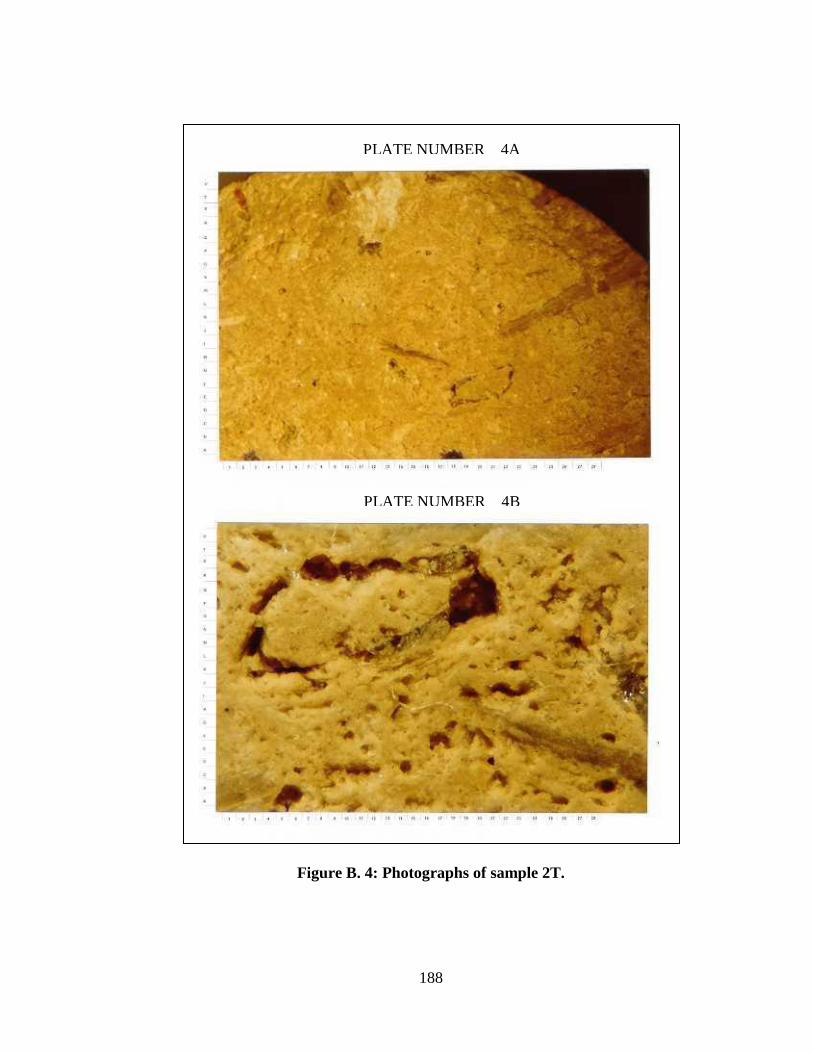
188
Figure B. 4: Photographs of sample 2T.
PLATE NUMBER 4A
PLATE NUMBER 4B

189
Figure B. 5: Thin section images of Sample 3T.
PLATE NUMBER 5A
PLATE NUMBER 5B

190
Figure B. 6: Photographs of sample 3T.
PLATE NUMBER 6A
PLATE NUMBER 6B

191
Figure B. 7: Thin section images of sample 4T.
PLATE NUMBER 7A
PLATE NUMBER 7B

192
Figure B. 8: Photographs of sample 4T.
PLATE NUMBER 8B
PLATE NUMBER 8A

193
Figure B. 9: Thin section images of sample 5T.
PLATE NUMBER 9B
PLATE NUMBER 9A

194
Figure B. 10: Photographs of sample 5T.
PLATE NUMBER 10A
PLATE NUMBER 10B

195
Figure B. 11: Thin section images of sample 6T.
PLATE NUMBER 11A
PLATE NUMBER 11B

196
Figure B. 12: Photographs of sample 6T.
PLATE NUMBER 12A
PLATE NUMBER 12B

197
APPENDIX C: CT IMAGES AND CT-POROSITY AND NMR T2
DISTRIBUTIONS
C.1. Group 3 Samples
Figure C. 1: Sample 1: (a) CT images (b) CT-porosity and NMR T2 distributions.

198
Figure C. 2: Sample 2: (a) CT images (b) CT-porosity and NMR T2 distributions.

199
Figure C. 3: Sample 3: (a) CT images (b) CT-porosity and NMR T2 distributions.

200
Figure C. 4: Sample 4: (a) CT images (b) CT-porosity and NMR T2 distributions.

201
Figure C. 5: Sample 5: (a) CT images (b) CT-porosity and NMR T2 distributions.

202
Figure C. 6: Sample 6: (a) CT images (b) CT-porosity and NMR T2 distributions.
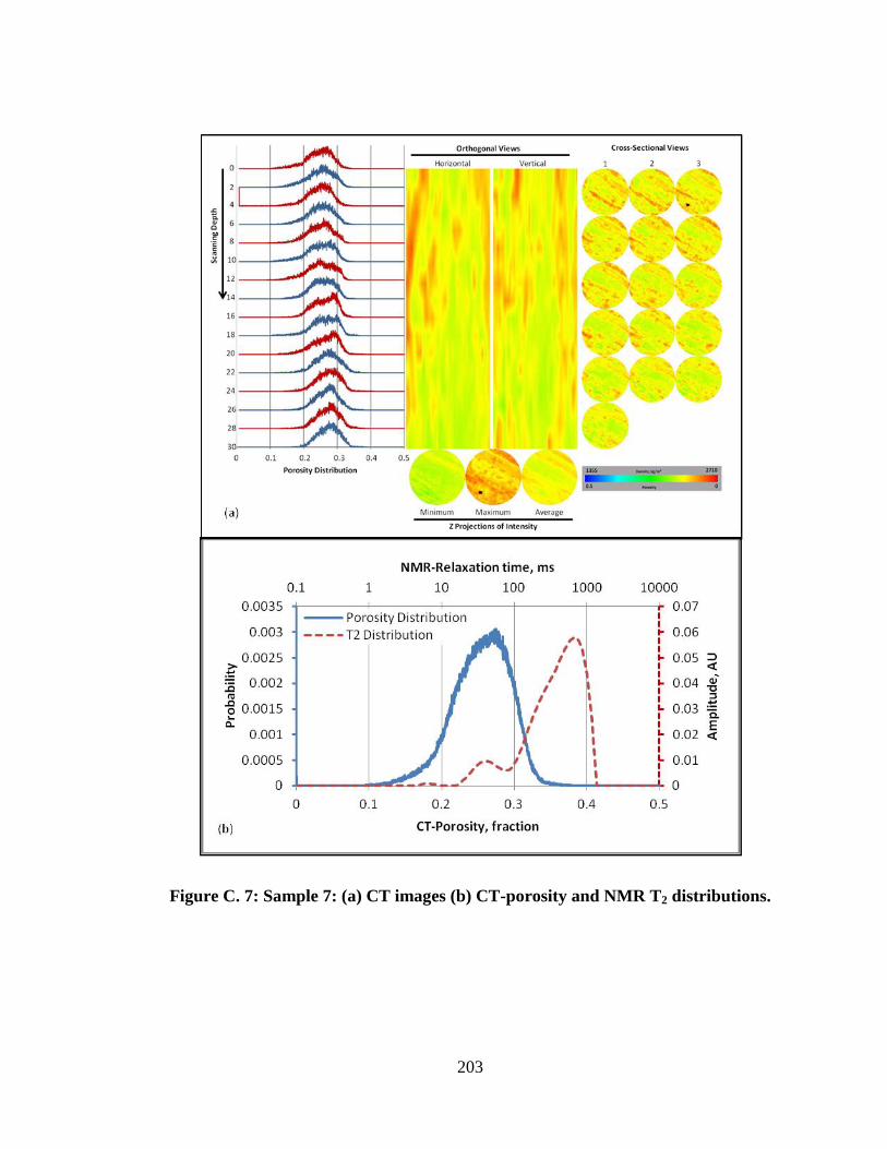
203
Figure C. 7: Sample 7: (a) CT images (b) CT-porosity and NMR T2 distributions.

204
Figure C. 8: Sample 8: (a) CT images (b) CT-porosity and NMR T2 distributions.

205
Figure C. 9: Sample 9: (a) CT images (b) CT-porosity and NMR T2 distributions.

206
C.2. Group 2 Samples
Figure C. 10: Sample 13: (a) CT images (b) CT-porosity and NMR T2 distributions.

207
Figure C. 11: Sample 14: (a) CT images (b) CT-porosity and NMR T2 distributions.

208
Figure C. 12: Sample 15: (a) CT images (b) CT-porosity and NMR T2 distributions.

209
Figure C. 13: Sample 16: (a) CT images (b) CT-porosity and NMR T2 distributions.
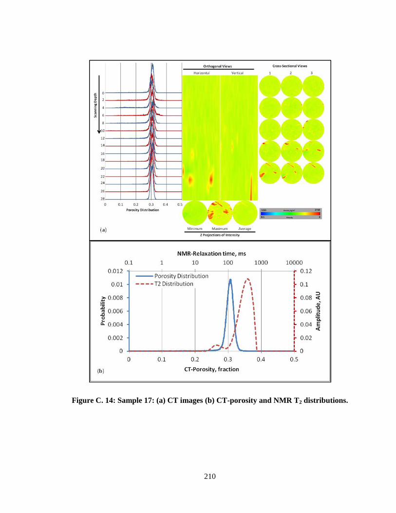
210
Figure C. 14: Sample 17: (a) CT images (b) CT-porosity and NMR T2 distributions.

211
Figure C. 15: Sample 18: (a) CT images (b) CT-porosity and NMR T2 distributions.

212
Figure C. 16: Sample 19: (a) CT images (b) CT-porosity and NMR T2 distributions.

213
Figure C. 17: Sample 20: (a) CT images (b) CT-porosity and NMR T2 distributions.

214
Figure C. 18: Sample 21: (a) CT images (b) CT-porosity and NMR T2 distributions.

215
Figure C. 19: Sample 22: (a) CT images (b) CT-porosity and NMR T2 distributions.

216
Figure C. 20: Sample 23: (a) CT images (b) CT-porosity and NMR T2 distributions.

217
Figure C. 21: Sample 24: (a) CT images (b) CT-porosity and NMR T2 distributions.
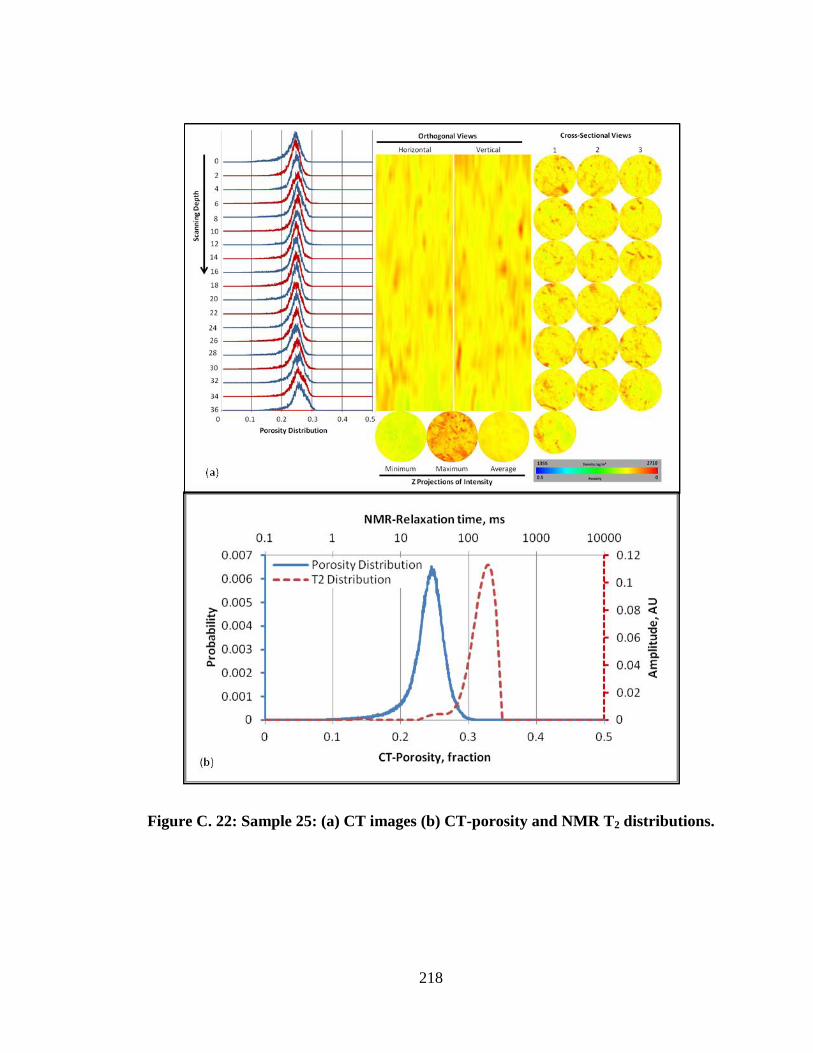
218
Figure C. 22: Sample 25: (a) CT images (b) CT-porosity and NMR T2 distributions.

219
Figure C. 23: Sample 26: (a) CT images (b) CT-porosity and NMR T2 distributions.

220
C.3. Group 1 Samples
Figure C. 24: Sample 32: (a) CT images (b) CT-porosity and NMR T2 distributions.

221
Figure C. 25: Sample 33: (a) CT images (b) CT-porosity and NMR T2 distributions.

222
Figure C. 26: Sample 34: (a) CT images (b) CT-porosity and NMR T2 distributions.

223
Figure C. 27: Sample 35: (a) CT images (b) CT-porosity and NMR T2 distributions.

224
Figure C. 28: Sample 36: (a) CT images (b) CT-porosity and NMR T2 distributions.

225
Figure C. 29: Sample 37: (a) CT images (b) CT-porosity and NMR T2 distributions.

226
Figure C. 30: Sample 38: (a) CT images (b) CT-porosity and NMR T2 distributions.

227
Figure C. 31: Sample 39: (a) CT images (b) CT-porosity and NMR T2 distributions.

228
C.4. Ungrouped Samples (Other1)
Figure C. 32: Sample 40: (a) CT images (b) CT-porosity and NMR T2 distributions.

229
Figure C. 33: Sample 41: (a) CT images (b) CT-porosity and NMR T2 distributions.

230
Figure C. 34: Sample 42: (a) CT images (b) CT-porosity and NMR T2 distributions.
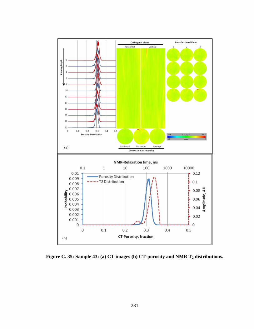
231
Figure C. 35: Sample 43: (a) CT images (b) CT-porosity and NMR T2 distributions.

232
C.5. Ungrouped Samples (Other2)
Figure C. 36: Sample 44: (a) CT images (b) CT-porosity and NMR T2 distributions.

233
Figure C. 37: Sample 45: (a) CT images (b) CT-porosity and NMR T2 distributions.

234
Figure C. 38: Sample 46: (a) CT images (b) CT-porosity and NMR T2 distributions.

235
Figure C. 39: Sample 47: (a) CT images (b) CT-porosity and NMR T2 distributions.

236
Figure C. 40: Sample 48: (a) CT images (b) CT-porosity and NMR T2 distributions.

237
Figure C. 41: Sample 49: (a) CT images (b) CT-porosity and NMR T2 distributions.

238
Figure C. 42: Sample 50: (a) CT images (b) CT-porosity and NMR T2 distributions

239
APPENDIX D: HISTORY MATCHING PARAMETERS
In order to history match the experimental data, Sendra varies the relative
permeability (Corey model) and the capillary pressure (Skjaeveland model) parameters
until a satisfactory match is achieved between the experimental and simulated data. In
this history matching study, the residual oil to gasflood (Sorg) was varied by Sendra in
order to correct for capillary end-effect contact. Table XXX shows the output parameters
from Sendra for the relative permeability and capillary pressure. These parameters are
defined somewhere else (Corey, 1954; Skjaeveland, 2000).
Table D. 1: Relative permeability and capillary pressure parameters used by Sendra
to history match the expemental data