Experimental Evaluation of a Low-Voltage Power Distribution Cable Model Based on FEM

IEEE TRANSACTIONS ON POWER DELIVERY, VOL. 22, NO. 3, JULY 2007 1455

Experimental Evaluation of a Low-VoltagePower Distribution Cable Model Based

on a Finite-Element ApproachGeorgios T. Andreou, Member, IEEE, and Dimitris P. Labridis, Senior Member, IEEE

Abstract—The authors presented in a former paper, a thoroughstudy concerning the electrical parameters of low-voltage powerdistribution cables widely used in residential networks in the fre-quency range up to 100 MHz. The calculation of the electrical pa-rameters was based on a finite-element procedure with respect tothe cables’ normal operational conditions. In this paper, a cablemodel is presented based on the above study. Approximations thatare made are analyzed and validated. Moreover, an experimentalsetup is used to validate the cable model, which includes variousand both single-path and multipath cable networks in order toachieve generality. Experimental results are analyzed, and theo-retical difficulties based on the cables’ nature are denoted.

Index Terms—Cable modeling, finite-element method (FEM),power-line communications.

I. INTRODUCTION

POWER-LINE communications technology has improvedrapidly over the last decade, resulting in complete and reli-

able systems, which can be used for communication over powerdistribution networks. This, however, is mainly the result ofgreat improvements in encoding and multiplexing techniques.On the other hand, several attempts have been made concerningthe proper modeling of low-voltage (LV) power distribution net-works in consumer premises as communication media. Many ofthe models proposed in the literature attempt to describe the ca-bles which comprise these networks by using their lumped ordistributed electrical parameters (i.e., their resistance , induc-tance , conductance , and capacitance per unit length[1]–[3]). Until recently, however, there was a lack of researchconcerning the theoretical estimation of these parameters.

In a former paper, the authors presented a thorough study con-cerning the exact estimation of the electrical parameters of LVpower distribution cables widely used in residential networks,in the frequency range up to 100 MHz [4]. A finite-element pro-cedure was used for the calculations, with respect to the cables’normal operational conditions. The results were compared sub-sequently with corresponding values obtained by theoretical cal-culation methods.

In this paper, a cable model is presented based on the afore-mentioned results. In the first part of this paper, the modelis described and the approximations made are explained andtested with respect to the cable’s characteristic impedance

Manuscript received July 20, 2006. Paper no. TPWRD-00395-2006.The authors are with the Department of Electrical and Computer Engineering,

Aristotle University of Thessaloniki, Thessaloniki 54124, Greece (e-mail: [email protected]; [email protected]).

Digital Object Identifier 10.1109/TPWRD.2007.900296

Fig. 1. Typical conductor arrangement for an NYM cable.

and propagation constant . In the second part, the experimentalsetup used for the validation of the model is presented. Thevarious cases examined are demonstrated, and the experimentalresults are analyzed and compared to the values obtained by thetheoretical model.

All results refer to a typical NYM 3 2.5-mm LV cable(Fig. 1) without limiting the generality of the model. The exam-ined frequency range reaches up to 30 MHz since this is the typ-ical frequency range utilized by the up-to-date power-line com-munications technology.

II. THEORETICAL CABLE MODEL

The cable model is based on properly estimated distributedelectrical parameters. We will consider the cable to be lossless;therefore, throughout the calculations, we will only use its in-ductance per unit length and capacitance per unit length .However, in this first part of the work we will also consider thecable’s resistance per unit length and conductance per unitlength so as to validate the above approximation. A more de-tailed study concerning the values used below can be found in[4].

A. Resistance Per Unit Length

The values used concerning the cable’s resistance per unitlength are calculated with the aforementioned finite-elementprocedure of [4]. The values are plotted versus the current fre-quency in Fig. 2.

B. Inductance Per Unit Length

Again, the values used concerning the cable’s inductance perunit length are calculated with the aforementioned finite-ele-ment procedure of [4]. The values are plotted versus the currentfrequency in Fig. 3.

0885-8977/$25.00 © 2007 IEEE

Authorized licensed use limited to: Sultan Qaboos University. Downloaded on October 25, 2009 at 08:16 from IEEE Xplore. Restrictions apply.

1456 IEEE TRANSACTIONS ON POWER DELIVERY, VOL. 22, NO. 3, JULY 2007

Fig. 2. Resistance per unit length for an NYM, 3� 2.5-mm cable.

Fig. 3. Inductance per unit length for an NYM, 3� 2.5-mm cable.

C. Capacitance Per Unit Length

As shown in [4], the capacitance per unit length of an LVpower distribution cable presents us with the most theoreticalproblems. We can account for the partial capacitances betweenthe conductors, but due to the absence of a metallic cover overthe conductors, the analytical calculation of the correspondingpartial capacitance between any of the conductors and earth ispractically impossible, as in this case the extent of the electro-static field is indeterminable [5]. The error factor, however, dueto the absence of the partial capacitances to earth in the theoret-ical calculations is generally small because of the cable’s smalldimensions compared to its distance from earth, as we will seelater.

The absence of a metallic cover over the conductors alsomakes the cable vulnerable to other adjacent electric-fieldsources, which can also not be accounted for. This will raiselocally the cable’s overall capacitance in a more or less randomway, producing some substantial narrowband deviations in ourresults.

The cable’s capacitance values used in the model presentedhere were calculated with the reciprocity theorem analyzed in[4]. The values for the permittivity of the dielectric separatingthe cable’s conductors (PVC as in [6]) can be found in [7],and are plotted versus frequency in Fig. 4. The correspondingcable’s capacitance-per-unit-length values are plotted versusfrequency in Fig. 5.

D. Conductance Per Unit Length

The values for the cable’s conductance per unit length arecalculated theoretically as explained in [4], and they are plottedversus frequency in Fig. 6.

Fig. 4. Dielectric permittivity for an NYM, 3� 2.5-mm cable.

Fig. 5. Capacitance per unit length for an NYM, 3� 2.5-mm cable.

Fig. 6. Conductance per unit length for an NYM, 3� 2.5-mm cable.

The corresponding values concerning the loss tangent ofthe cable’s dielectric material can also be found in [7] and areplotted versus frequency in Fig. 7.

E. Validation of Approximations

Next, we will examine the variation in the cable’s character-istic impedance and propagation constant because of theapproximation made for the model presented here, regarding thecable as lossless.

The characteristic impedance of a uniform transmission linecan be generally calculated with (1) [8] as follows:

(1)


ANDREOU AND LABRIDIS: EXPERIMENTAL EVALUATION OF A CABLE MODEL 1457

Fig. 7. Dielectric loss tangent for an NYM, 3� 2.5-mm cable.

Fig. 8. Modulus of the characteristic impedance of an NYM, 3� 2.5-mmcable when considered lossless and lossy, respectively.

Fig. 9. Phase of the characteristic impedance of an NYM, 3� 2.5-mm cablewhen considered lossless and lossy, respectively.

When and are small or when the frequency is large, sothat and , (1) reduces to [8]

(2)

Figs. 8 and 9 show the variation of the modulus and phase,respectively, of the cable’s characteristic impedance, when thecable is considered as a lossy or lossless transmission line. Thevalues for the respective cable’s electrical parameters are takenas explained in the previous section of this paper.

For very low frequencies (up to about 10 kHz), the cablecannot be considered as a lossless transmission line, because

the condition does not hold. This frequency range istherefore omitted in the above figures, so as to improve clarityin the remaining frequency range.

As shown in Figs. 8 and 9, the cable can be very accuratelyconsidered as a lossless transmission line above the frequency of10 kHz, as the deviation for the characteristic impedance’s mod-ulus remains below 0.33% for the whole remaining frequencyrange. The respective phase deviation remains for the same fre-quency range below 1.4 .

F. Input Impedance of Lossless Transmission Line

Matick shows in [8] that the impedance of a transmission linenot terminated in its characteristic impedance, at any point andlooking toward the load, can be calculated with (3)

(3)

where is the characteristic impedance of the transmissionline, is its termination resistance, is its length, and is itspropagation constant.

If we let go to zero, determining the input impedance of thetotal line, (3) is then simplified to [8]

(4)

For a lossless line, it will be [8]

(5)

where is the wavelength of the applied frequency. Substi-tuting (5) into (4) will yield

(6)

Equation (6) was used to validate the results obtained by theabove theoretical analysis compared to the experimental resultsthat follow.

III. VALIDATION OF THEORETICAL MODEL

A. Experimental Setup

The experimental setup used to validate the theoretical anal-ysis was built in regard to the normal operational conditions ofthe cable under study in a residential LV power distribution net-work. Therefore, a number of plastic cable ducts were fixed onan ordinary wall (without existing internal wiring), simulatingthe cable path of an ordinary residential power circuit. The ductarrangement appears in Fig. 10.

Within these ducts, a number of different cable configurationswere used for the measurement procedure. During the experi-ments, an HP 8714ES network analyzer was used to measure theinput impedance of the various circuits formed in the ducts by



Fig. 10. Duct arrangement for experimental setup.

Fig. 11. Modulus of input impedance for Case 1: single NYM 3� 2.5-mmcable, 1-m length.

the cables under study. The lower frequency limit of the mea-surements was set to 300 kHz, which was the lower limit ofthe network-analyzer frequency range. The measurements wereconducted up to the frequency of 30 MHz, a typical power-linecommunications upper frequency limit.

The network analyzer was calibrated prior to any measure-ment set with the HP 85032E Type N calibration kit. Each cal-ibration procedure included the configuration of the networkanalyzer with three standardized terminations implementing anopen circuit, a short circuit, and a 50- termination resistance,respectively.

For every measurement, conductors 1 and 2 (Fig. 1) at a freecable end were attached to one port of the network analyzer,whereas conductor 3 was left open. The other cable ends wereterminated with 50- termination resistances.

In the following paragraphs, various cases used during themeasurement procedure are analyzed, and the results obtainedare presented and compared to the respective theoretical calcu-lations.

B. Case A: Single Paths

The first measurements regarding single cables were laid in-side the ducts. The cable lengths used were 1, 2, and 6 m. Thecable ends not attached to the network analyzer were terminatedwith a 50- termination resistance. In Figs.11–16, experimentalresults are presented and compared to corresponding theoreticalcalculations for three cases (Case 1, Case 2, and Case 3), cor-responding to the above three cable lengths (1, 2, and 6 m), re-spectively. Two figures correspond to every case, one showingthe modulus of the cable’s input impedance and one showingthe respective phase.

In most cases, the above figures show an acceptable conver-gence between theoretical and experimental results. However,

Fig. 12. Phase of input impedance for Case 1: single NYM 3� 2.5-mm cable,1-m length.



there are small frequency ranges where the cable shows a sig-nificant capacitive behavior not anticipated by theory. The ex-planation lies in the aforementioned theoretical inadequacy toestimate accurately the cable’s capacitance to earth and to theadjacent electric-field sources, which exist in any residentialbuilding. As an example, the greatest observed deviation in theabove figures [about 80 or 70% in the modulus of the inputimpedance of a 2-m-long NYM, 3 2.5-mm cable at the fre-quency of 27.5 MHz (Fig. 13) can be simulated with a respectiveincrease in the cable’s overall capacitance at the vicinity of thatfrequency, which can be caused by an equivalent outer capaci-tance within the order of 0.75 nF at 27.5 MHz].

Moreover, it can also be observed that the deviation of experi-mental results as compared to theoretical calculations decreaseswith the increase of the cable length, because of the respective


ANDREOU AND LABRIDIS: EXPERIMENTAL EVALUATION OF A CABLE MODEL 1459



Fig. 17. Cable arrangement for Case 4.


increase of the cable’s inductance and capacitance, which re-sults in the reduction of the influence of adjacent electric-fieldsources to the cable’s impedance.

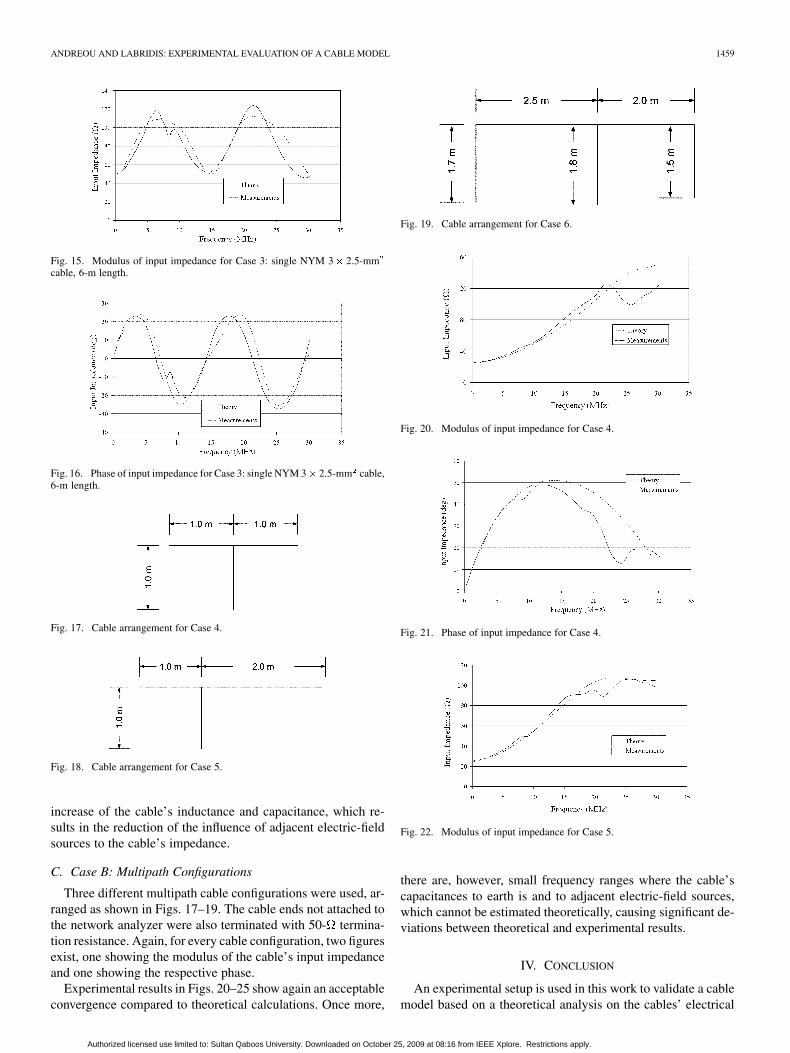
C. Case B: Multipath Configurations

Three different multipath cable configurations were used, ar-ranged as shown in Figs. 17–19. The cable ends not attached tothe network analyzer were also terminated with 50- termina-tion resistance. Again, for every cable configuration, two figuresexist, one showing the modulus of the cable’s input impedanceand one showing the respective phase.

Experimental results in Figs. 20–25 show again an acceptableconvergence compared to theoretical calculations. Once more,


Fig. 20. Modulus of input impedance for Case 4.

Fig. 21. Phase of input impedance for Case 4.


there are, however, small frequency ranges where the cable’scapacitances to earth is and to adjacent electric-field sources,which cannot be estimated theoretically, causing significant de-viations between theoretical and experimental results.

IV. CONCLUSION

An experimental setup is used in this work to validate a cablemodel based on a theoretical analysis on the cables’ electrical






parameters conducted by the authors in a former work. The fre-quency range used is that of a typical power-line communica-tions system. At first, the values used for the electrical param-eters of the cable type under study are presented. The approx-imations used in the model are analyzed and validated. Subse-quently, the experimental setup is presented, and both simpleand multipath cable configurations are used to validate the the-oretical analysis.

Results show an acceptable convergence between theoryand experiments concerning the various configurations’ inputimpedance. There are, however, small frequency ranges with asubstantial deviation due to the capacitive behavior of the cablenot anticipated by theory. Nevertheless, this phenomenon wasgenerally expected to appear because of the inherent theoreticalinadequacy to accurately estimate the cable’s capacitance toearth as well as to other adjacent electric-field sources.

REFERENCES

[1] D. Anastasiadou and T. Antonakopoulos, “An experimental setup forcharacterizing the residential power grid variable behavior,” presentedat the 6th Int. Symp. Power-Line Communications and Its Applica-tions, Athens, Greece, 2002.

[2] I. C. Papaleonidopoulos, C. G. Karagiannopoulos, N. J. Theodorou, C.E. Anagnostopoulos, and I. E. Anagnostopoulos, “Modelling of indoorlow voltage power-line cables in the high frequency range,” presentedat the 6th Int. Symp. Power-Line Communications and Its Applica-tions, Athens, Greece, 2002.

[3] M. Zimmermann and K. Dostert, “A multipath model for the power-line channel,” IEEE Trans. Commun., vol. 50, no. 4, pp. 553–559, Apr.2002.

[4] G. T. Andreou and D. P. Labridis, “Electrical parameters oflow-voltage power distribution cables used for power-line com-munications,” IEEE Trans. Power Del., vol. 22, no. 2, pp. 879–886,Apr. 2007.

[5] L. Heinhold, Power Cables and their Application–Part 1. Berlin,Germany: Siemens Aktiengesellschaft, 1993, p. 331.

[6] R. Arora and W. Mosch, High Voltage Insulation Engineering. NewDelhi, India: New Age International (P) Ltd., 2004, p. 242.

[7] A. von Hippel, Dielectric Materials and Applications. Norwood,MA: Artech House, 1994, pp. 329–330.

[8] R. E. Matick, Transmission Lines for Digital and Communication Net-works. New York: IEEE Press, 1995, pp. 34–35.

Georgios T. Andreou (S’98–A’02–M’04) was born in Thessaloniki, Greece,on August 16, 1976. He received the Dipl.-Eng. degree from the Department ofElectrical and Computer Engineering at the Aristotle University of Thessaloniki,Thessaloniki, in 2000.

Since 2001, he has been a postgraduate student in the Department of Electricaland Computer Engineering at the Aristotle University of Thessaloniki. His spe-cial interests are power system analysis and power-line communications.

Dimitris P. Labridis (S’88–M’90–SM’00) was born in Thessaloniki, Greece,on July 26, 1958. He received the Dipl.-Eng. and Ph.D. degrees from the De-partment of Electrical Engineering at the Aristotle University of Thessaloniki,Thessaloniki, in 1981 and 1989, respectively.

During 1982–2001, he was a Research Assistant and then a Lecturer and As-sistant Professor at the Department of Electrical Engineering, Aristotle Univer-sity of Thessaloniki. Since 2001, he has been Associate Professor at the same de-partment. His special interests are power system analysis with special emphasison the simulation of transmission and distribution systems, electromagnetic andthermal field analysis, numerical methods in engineering, artificial intelligenceapplications in power systems, and power-line communications.


Documents

Experimental Evaluation of a Low-Voltage Power Distribution Cable Model Based on FEM