Experimental Estimation of Heterogeneous Treatment Effects Related to Self-Selection

Brian J. Gaines University of IllinoisJames H. Kuklinski University of Illinois*

Abstract

Social scientists widely regard the random-assignment experiment as the gold standard for

making causal inferences about the world. We argue that it can be improved. For situations in

which self-selection and heterogeneity of treatment effects exist, an alternative experimental

design that retains random assignment to treatment or control and supplements it with some self-

selection of condition offers a clear advantage. It reveals the average treatment effect while also

allowing estimation of the distinct effects of the treatment on those apt and inapt to experience

the treatment outside the experimental context.

* Brian J. Gaines is an Associate Professor and James H. Kuklinski is the Matthew T. McClure Professor at the University of Illinois, where they both hold appointments in the Department of Political Science and at the Institute of Government and Public Affairs. Contact bjgaines@illinois.edu, kuklinsk@illinois.edu or either author at IGPA / 1007 W. Nevada St. / Urbana, IL 61801. We are very grateful to numerous audiences and individuals for helpful advice, including but not limited to Jake Bowers, Jason Coronel, Tiberiu Dragu, Jamie Druckman, Mark Frederickson, Matthew Hayes, Jude Hays, Rebecca Morton, Tom Rudolph, Jas Sekhon, Lynn Vavreck, the editor, and four anonymous referees. We are especially indebted to Don Green for many greatly helpful suggestions. The data analyzed in Table 2 can be accessed as a Stata file at https://netfiles.uiuc.edu/bjgaines/replication%20data/.

1

Political scientists increasingly view the random-assignment experiment as not merely

acceptable, but, in fact, optimal when one's goal is to test simple theories of the form X causes Y.

Not all phenomena of interest are amenable to experimental simulation, of course, although

creative researchers have expanded the substantive boundaries to which they apply experiments.

As a result, experimentalists and users of observational data have begun to address the same

topics.1 Druckman et al. (2006: 629) observe that experimenters are increasingly entering the

fray when observational studies, with their attendant problems such as endogenous causality and

omitted variable bias, fail to reach consensus. Iyengar and Kinder’s study of media priming and

framing effects (1987), for example, literally ended the “minimal media effects” debate.

Like Iyengar and Kinder, most experimentalists seek to generate results with broad

applicability. In the words of Shadish, Cook, and Campbell (2002: 18-19), “most experiments

are highly local and particularized, but have general aspirations.” Even when subjects are not

simple random samples from identifiable populations, experimenters very rarely draw

conclusions limited to only the single set of observations at hand. Absent a capacity for causal

inference, many social science experiments would have plainly limited value.

We argue that the prototypical randomized experiment, the purported gold standard for

identifying cause and effect, falls short when the treatment under study is prone to self-selection

in the population and the researcher aims to draw meaningful inferences about its effect. A

design that retains random assignment while accounting for the endogenous selection into or out

of treatment in the external world can then be beneficial.

In essence, an experiment featuring only randomized treatment answers questions of the

form, “How would X work on Y in the event that everyone were exposed to X?” When making

inferences about situations where self-selection into and out of the causal factor occurs, the

2

experiment ideally will answer two additional questions: “How does X affect Y for those who

choose to expose themselves to X?” and “How would X affect Y for those who avoid X?”

We propose a novel experimental design that answers all three questions. It retains

randomized treatment, and its concomitant, an estimate of the overall average treatment effect,

and also generates estimates of the potentially distinct treatment effects on those most and least

likely to be treated outside the experimental context. In other words, it decomposes the average

treatment effect into two important components, the empirical treatment effect and a merely

potential treatment effect for those not normally treated. The simple modification entails random

assignment not only to treatment and control, but also to a third condition, wherein subjects self-

select into or out of the treatment.

We do not recommend this design for all experimental studies. Self-selection is not

present in all situations suitable for experimental study, and the design is more easily

implemented in survey and laboratory than in field experiments. In the former, the researcher

typically can confirm that subjects assigned to treatment were actually treated, and can also

undertake manipulation checks to test whether the treatment took effect. One difficulty with

incorporating self-selection into field experiments arises from noncompliance wherein some

individuals defy their random assignments to treatment or control status.

Most fundamentally, we do not propose to reduce the importance of internal validity to

experimental research. On the contrary, randomization and internal validity are pivotal to our

proposal, and we demonstrate that internal validity can be retained while improving external

validity.2 Our suggestion is not to eschew random assignment, but to harness it for studying

selection and its impact on treatment effects.

3

Although focused specifically on experiments and causal inference, this paper contributes

more generally to a growing, diverse literature whose authors seek to strengthen the question-

design connection. We have in mind, for example, Signorino and Yilmaz’s work (2003) on

proper specifications of statistical models for situations where agents interact strategically,

Granato, Lo, and Wong’s proposals (2010) to unify formal theories and statistical models, and

Braumoeller and Goertz’s (2000) formulation of statistical models to test theories that posit

necessary and sufficient conditions. In the same vein, we seek to facilitate better communication

across users of observational and experimental data. Progress requires that all participants pose

their questions precisely and explicitly, and that individual researchers use methodologies

commensurate with the questions they ask. These are topics that should interest all social

scientists, regardless of whether or not they use experiments in their own research.

Our discussion proceeds as follows. The first section sets forth a rationale for revising the

classic experiment, using as its motivating illustration the study of the relationship between

negative campaigns and turnout. It also enumerates other areas of inquiry where the likelihood of

self-selection poses a threat to experimentally based inference. The second section focuses on

logics, first of the classic experiment, then of our alternative design that accounts for

heterogeneity arising from self-selection while retaining the advantages that accrue from

randomization. We also discuss logistical difficulties of incorporating self-selection into a field

experiment. A third section introduces a numerical example to clarify the proposed design. Using

a hypothetical population for whom relevant parameters are known, we show how the expanded

design generates more informative inferences than a simple random-assignment experiment

does. We also investigate how imperfect experimental simulation of external selection behavior

affects the estimated treatment effect. A fourth section briefly discusses logistical challenges

4

associated with incorporating self-selection into experiments. Finally, we present results of a

pilot study of how exposure to negative campaign materials affects reactions to candidates.

The Study of Negative Campaign Ads and Voting Turnout

Does campaign negativity affect turnout? The heated and still unresolved debate on this

question has extended far beyond the boundaries of academic political science. Advocates of

campaign finance reform cited research showing that negative campaign advertising reduced

turnout; later, scholarly criticisms of that work entered the realm of public policy debates and

even court proceedings, in McConnell v. FEC.

Political scientists have reported three mutually exclusive and exhaustive findings about

the effects of negative television advertisements ("ads" hereafter) on voting turnout: they depress

it, enhance it, and have no effect at all. And they have used three distinct approaches to generate

these disparate results: conducting experiments in which exposure to negative ads is the key

treatment; analyzing aggregate data, including variables characterizing the degree of negativity

of various contests; and, analyzing survey data, including self reports of ad exposure.3

The thesis that negative ads reduce turnout is rooted in a prominent experimental study

(Ansolabehere et al. 1994; also Ansolabehere and Iyengar 1995). The researchers randomly

assigned a convenience sample of potential Los Angeles area voters to one of three treatments.

Subjects watched a newscast, embedded in which were a negative ad, a positive ad, or, as the

control, a (positive) non-political product ad. The ads came from the actual campaigns of

candidates running for governor and the United States Senate in California in 1992. In brief, the

authors found effects of roughly 5 percentage points; those who saw a positive ad were about 2.5

points more likely to say they would vote than those in the control condition, while those who

saw a negative ad were around 2.5 points less likely to say they would vote (1994, 833).

5

Ansolabehere et al. (1999) then analyzed aggregate data on 1992 U.S. Senate elections to

buttress their experimentally based inferences.

Political scientists have offered a variety of explanations for the wide-ranging results and

conclusions across studies.4 Critics of the experimental results point to unrealistically strong

laboratory treatments; critics of survey-based research focus predominantly on measurement

error, especially the unreliability of respondents’ self-reported recalls of exposure; and critics of

studies using aggregate data center on poor measures of advertising tone and volume, and,

especially, possible spurious correlations.

Strikingly, for all of the work done on the subject, we know no study that assesses the

logic of using a random-assignment experiment to make valid inferences about the effects of

campaign ads outside the experimental context. Current thinking applauds the use of such

experiments, putting aside the possibility of overly strong treatments, for the very reason that

randomization equalizes the effects of possible confounds across conditions and, more directly

relevant here, completely eliminates selection effects. The random-assignment experiment, in

short, produces clean, readily interpretable results about cause and effect.

Why, then, even consider introducing a self-selection condition into the classical random-

assignment experiment? Consider how random assignment eliminates self-selection. Some

people in the population who would expose themselves to the treatment (a negative ad) do not

get it, while others who would never expose themselves do. This deliberate, coercive elimination

of self-selection can become a problem for the experimenter aiming to infer how the treatment

affects the response variable among people outside the experimental context. The problem arises

when some people select into and others out of the treatment, and the treatment’s effects,

whether realized or not, differ between those who select in and those who select out. Then, the

6

estimated treatment effect, the overall average effect of a negative ad on voting turnout, exists

only within the random-assignment experiment itself.5

We can restate the problem in terms of a discrepancy between questions researchers

intend to ask and those they actually answer. Garfinkel (1981) argues convincingly that social

scientists all too often formulate research questions that lack clarity and precision. This failure

obscures the meaning of any single study’s results and hampers substantive communication

across studies. Research on the topic of negative campaign ads and voting turnout includes

observational and experimental studies. All contributors seek to make inferences about the causal

effects of ads in real campaigns. A single, sometimes explicitly stated, question—How do

negative campaign ads affect voting turnout?—would seem to guide them.

On reflection, that question is too vague. The typical observational study implicitly

addresses this question: what are the effects of negative campaign ads given that some people are

exposed to them and others are not? The random-assignment experiment addresses a different

question: what would be the effects of negative campaign ads if everyone watched them? Each

question is important, but the two are distinct. Thus, observational and experimental studies

should not generate the same results unless, outside the experiment, self-selection does not occur

or ads identically affect individuals who are and are not exposed, or, inside the experiment,

selection to watch or not watch ads is incorporated in the design.6

We continue to use campaign negativity as a running example below, although many

other topics and phenomena studied with experiments are also prone to self-selection. The

investigation of source effects, for instance, is a staple of political psychology and political

communication. Researchers routinely ask whether and how hearing different framings of issues

affects people’s beliefs and attitudes, including their willingness to tolerate people who differ

7

from them (Chong and Druckman 2007; Kinder and Sanders 1990; Nelson, Clawson, and Oxley

1997; Sniderman and Theriault 2004); or whether watching different newscasts—CNN versus

FOX News, for example—causes people to react differently to unfolding events; or how

incivility among politicians affects viewers’ attitudes about politics (Mutz 2007). Political

scientists are increasingly using experiments to study the effects of various deliberation

structures on participants’ acceptance of the collective outcomes, and whether participating in a

deliberative process that requires people openly to justify their beliefs and opinions changes

those beliefs and opinions (see, for example, Sulkin and Simon.2002).

In these instances and others, researchers seek to make causal inferences that apply

beyond the specific experimental context; thus all of the cautions we raised with respect to the

study of negative campaign ads and voting turnout apply here as well. Generally, the average

effect detected in the classic random assignment experiment mixes together a real-world

phenomenon (the treatment's effect on those who are, away from the experimental simulation,

treated) and a hypothetical one that exists only within the experiment itself (its effect on those

who are not generally treated away from the experimental simulation). In turn, the estimated

experimental effect will be of limited value to the researcher.

Logical Basis

For decades, most data analysis in political science (and other sciences) was motivated by

a rather casual notion of causality. Observational data were the modal variety, and data analysts

usually took for granted that strong associations therein could be interpreted as causal findings,

notwithstanding the ubiquity of the slogan “correlation is not causation.”

Eventually, however, skepticism about the value of observational data for making causal

claims began to makes its way from statistics to the natural and social sciences. As Holland

8

(1986) emphasized, conventional statistical analysis of observational data can answer only the

question, “Which of a set of observable, potential causes are associated with an effect?” To

answer the distinct question, “What are the effects of a cause (treatment)?” requires

randomization and control of the treatment.

The logic of the random-assignment experiment, meanwhile, is not quite so straight-

forward as to require no exposition at all. A treatment’s effect, in the case of a dichotomous

treatment, is the simple difference, (Yi | t = 1) - (Yi | t = 0), where the variable Y describes some

phenomenon of interest. In most contexts, this difference is purely hypothetical, since the

researcher cannot observe multiple outcomes (realizations of the variable of interest) for any

given unit. Hence, experimentalists traditionally estimate the unobservable treatment effect by

comparing averages of groups. That is, they use (Y|t=1¿−(Y|t=0¿ to estimate the quantity

E((Yi | t = 1) - (Yi | t = 0)), usually labeling the former “the treatment effect,” although “average

treatment effect” more aptly describes the difference-of-means estimate, since the averages of

the treatment and control groups mask within-group heterogeneity.7

We have proposed that one particular form of heterogeneity, between those likely to be

treated outside of experiments and those not, holds special importance. We are not the first to

broach this point. Gerber and Green write: “The concept of the average treatment effect

implicitly acknowledges the fact that the treatment effect may vary across individuals in

systematic ways. One of the most important patterns of variation in τi [their parameter for

treatment effect] occurs when the treatment effect is especially large (or small) among those who

seek out a given treatment. In such cases, the average treatment effect in the population may be

quite different from the average treatment effect among those who actually receive the

9

treatment” (2008: 362). The very possibility of such heterogeneity signals the importance of

incorporating self-selection into the experimental design.

To see this point more clearly and more generally, assume the following: Y is a

dichotomous variable that measures a behavior of interest; is the proportion of the population

that self-selects into a treatment when given the choice; in the absence of treatment, self-

selectors have probability ys and non-self-selectors have probability yn of exhibiting the behavior

of interest; the treatment effects, which alter the probabilities and are not assumed to be equal,

are ts for self-selectors and tn for non-self-selectors. Finally, assume for now that the process of

selecting treatment can be perfectly simulated within the experiment.8

The classical random-assignment experiment, depicted on the bottom branch of Figure 1,

generates two means (proportions) whose difference is the average treatment effect,

α ( t s )+(1−α )( tn ) . Note that α is unknown, and thus separating ts and tn is not possible.

Randomization balances (in expectation) heterogeneity in baseline probabilities across the

treatment and control groups, so that the ys and yn terms cancel in subtraction. The estimated

treatment effect is a weighted average, but the weights and the distinct treatment effects remain

unknown to the experimenter.

A simple variation on the traditional experimental design allows estimation of all three

treatment effects: the average effect and the effects among selectors and non-selectors. Figure 1

shows that it consists of randomly assigning subjects to one of the three conditions just noted, the

usual treatment and control conditions, plus a self-selection condition in which subjects

themselves choose whether or not to receive the treatment.9 Random assignment ensures that the

mixtures of self-selectors and non-self-selectors will be identical, in expectation, in all three

randomly formed groups.

10

The figure shows, for each of the three conditions, the expected proportions exhibiting

the behavior of interest (the expected value of the mean of outcome variable Y). Selection within

the self-selection group is not random, and simple algebra reveals the analytic usefulness of this

fact. The expected value for the whole, randomly constituted group assigned to the selection

condition is a weighted average of two probabilities, the probability given treatment for the

selectors and the probability given no treatment for the non-selectors. Allowing some subjects to

choose their treatments directly generates an estimate of the proportion of the population that

self-selects into treatment. The researcher can then use that estimate to recover estimates of the

two potentially distinct treatment effects, unpacking any heterogeneity between those inclined

and those disinclined to be treated:

t s=Y S−Y C

α

and

tn=Y T−Y S

1− α

where the upper-case subscripts designate the three randomly formed groups, C(ontrol),

T(reatment), and S(elf-selectors).

(Figure 1 about here)

Obtaining standard errors for t s and tn is not trivial. Because α is itself an estimate,

these estimators are non-linear functions of estimates, and ratio bias is thus a concern. The two

estimators include some common terms, and will normally be correlated. One common approach

to dealing with non-linear combinations of parameters of this type is the delta method for

approximating the distributions and variances (Cameron and Trivedi 2005: 231-32).10

Bootstrapping is another possibility.

11

An astute observer might have observed that the formulae presented immediately above

resemble a popular calculation to correct for the non-treatment of subjects assigned to treatment

in field experiments, one form of the problem commonly known as noncompliance (Angrist et al.

1996, Gerber and Green 1999). The similarity is not accidental, and comparing the purposes and

similarities of that calculation with ours reveals some unique logical challenges associated with

incorporating self-selection into field experiments.

When field experimenters observe unintended non-treatment, they commonly divide the

difference between the dependent variable for the treatment and control groups by the proportion

of the group assigned to be treated that was, in fact, successfully treated. The logic is that

subjects can be regarded as falling into two types, the easy-to-reach and the hard-to-reach. The

types might differ on the dependent variable when untreated, and also in the effect of the

treatment on their behavior. If the contacting process is assumed to be a perfect classifier of type,

then the point of the adjustment can be seen in the expected value of this estimator (mimicking

the notation above, but with “e” designating easy-to-reach and “h” hard-to-reach, and γ

designating the proportion of the population that is type “e”):

E( t¿¿e )=E( Y T−Y C

γ )= γ ( ye+ te )+(1−γ ) yh−γ ye−(1−γ ) yh

γ=t e¿

Two key assumptions underlie this calculation: first, randomization guarantees that, in

expectation, the groups assigned to treatment and control are identical in composition; and,

second, noncompliance is limited to observable non-treatment of those assigned to treatment, so

that gamma is estimated without bias.

This calculation differs from our proposed hybrid design in that it does not recover any

estimate of either th or of the average of the two treatment effects for the two types. Although

authors often describe the resulting quantity as an estimate of “the” treatment effect, the entire

12

process of adjustment is premised on there being two potentially different treatment effects, only

one of which is estimated. In the event that the easy and hard types can be regarded as identical

to selectors and non-selectors, a field experimenter who follows standard practice produces an

estimate of what we have termed the treatment effect for selectors only. Assuming that non-

selectors and the hard-to-reach are not identical complicates an already difficult problem.

All this said, we refrain from stating absolutely that self-selection can never be

incorporated into field studies. Scholars are creative, and they have made notable progress in

overcoming or compensating for noncompliance. It would be imprudent to assume that today’s

limitations will apply tomorrow.

In summary, from a purely logical perspective, incorporating self-selection into the

random-assignment experiment adds considerable analytical leverage. Random assignment of the

treatment isolates the treatment effect, but at the cost of weakening the capacity to make

inferences about an external world in which individuals might vary in their exposures to a

treatment or in their responses to treatment, in the event of exposure. Including self-selection

garners empirical validity, but it also conflates treatment and self-selection effects, thus

introducing the very problem that besets observational studies. But combining random

assignment and self-selection should generate data that, when correctly analyzed, reveal more

about the phenomenon under study than the classic random-assignment experiment.

Numerical Illustration

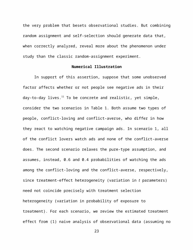
In support of this assertion, suppose that some unobserved factor affects whether or not

people see negative ads in their day-to-day lives.11 To be concrete and realistic, yet simple,

consider the two scenarios in Table 1. Both assume two types of people, conflict-loving and

conflict-averse, who differ in how they react to watching negative campaign ads. In scenario 1,

13

all of the conflict lovers watch ads and none of the conflict-averse does. The second scenario

relaxes the pure-type assumption, and assumes, instead, 0.6 and 0.4 probabilities of watching the

ads among the conflict-loving and the conflict-averse, respectively, since treatment-effect

heterogeneity (variation in t parameters) need not coincide precisely with treatment selection

heterogeneity (variation in probability of exposure to treatment). For each scenario, we review

the estimated treatment effect from (1) naive analysis of observational data (assuming no

measurement error), (2) a random-assignment experiment, and (3) an experiment of the sort we

advocate, combining random assignment and self-selection.

(Table 1 about here)

In scenario 1, only the mobilizing effect occurs in the real world, and naïve observational

studies, in attributing the full difference in turnout rates to ad exposure, would estimate, on

average, a +13% point effect, based on (roughly) 50% turnout among those who did not watch

the ads and (roughly) 63% among those who did. This estimate conflates the true treatment effect

for conflict-loving viewers (+5%) and the difference in baseline voting rates (+8%) between

those who watch and those who do not watch the ads.

If V is the proportion reporting (truthfully) that they intend to vote, then a random-

assignment experiment would generate an expected-treatment-effect estimate of E(V|T)-E(V|C):

(0.40)(0.58+0.05)+(0.60)(0.50-0.10) - (0.40)(0.58)+(0.60)(0.50) = 0.52-0.48 = -0.04. This is a

correct estimate of the average treatment effect were everyone to watch the ads. Randomization

corrects for the different baseline rates, and the estimated treatment effect is a weighted average

of the two possible treatment effects, where the weights are population shares. One should not

conclude, however, that negative ads reduce turnout in the external world. The random-

14

assignment experiment demonstrates, rather, that universal exposure to the ads, if it existed,

would reduce turnout.

A self-selection experiment generates this same overall-average estimate, but also two

additional estimates, as described above. Assume, for now, that implementing selection is

unproblematic (we return to this important practical question below). For watchers, the expected

value for the estimated treatment effect is E(V|S)-E(V|C)/E(α) = (0.552-0.532)/0.4 = 0.05; for

non-watchers, it is E(V|T)-E(V|S)/(1-E(α)) = (0.492-0.552)/(0.60) = -0.10. Both treatment-effect

parameters are estimated without bias. Allowing some respondents to select treatment thus

generates information on a real-world counterfactual, permitting an estimate that the ads, if

viewed, would reduce the probability of voting by about 10 percentage points among those who

do not, in fact, watch them.

There are, in these extra estimates, multiple answers to the question, “What is the effect

of negative ads in the real world?” The estimated treatment effect for watchers provides one

answer: “On average, viewing negative ads increases the probability of voting by about 5 points

among those who view them.” Because the experiment also provides an estimate of the

proportion of people that watch ads, it can provide a slightly fuller answer to the question, which

continues, “Since about 40% of the population chooses to watch ads, the net effect is a 2-

percentage point rise in turnout.”12 Finally, as with the random-assignment experiment, the data

provide an estimate of what negative-ad viewing would do in a world with universal treatment.

Sometimes this counterfactual will be of interest, sometimes not. By combining randomization

and self-selection, the experiment avoids the mistake of the simple observational study (and of

the self-selection module in isolation), of attributing all difference between watchers and non-

15

watchers to the watching. It also escapes the limitations of the random-assignment design, by

attending to an important variety of heterogeneity in the treatment effect.

Figure 2 shows values from 500 simulations of the estimates for this scenario, each with

N=1000. It provides a sense for how much uncertainty arises from sampling for the ratio

estimators, and how the two estimators can be correlated. In this case, the mode is slightly off the

true values, but more striking is the dispersion, suggesting that sample size is more important

than in a more conventional estimation problem.

(Figure 2 about here)

The second scenario in Table 1 slightly complicates the data-generating parameters.

Types are no longer pure, so both watchers and non-watchers are, in any given instance, mixtures

of the two fundamental types. Hence, treatment-effect heterogeneity now exists within the

observable, behavioral types, those who watch ads and those who do not.

The naive estimate would now be about a 1% demobilization effect. This figure conflates

two differences between watchers and non-watchers, their tendencies to watch (or not watch) the

ads, and their reactions to the ads. The random-assignment portion of the experiment ignores

real-world exposure, the only aspect of the first scenario that was altered, so it produces precisely

the same estimate as above, still best understood as the potential effect of negative ads, given

universal exposure. The self-selection experiment generates estimates of ts and tn that shrink to

-0.025 and -0.054, respectively. These values are no longer exact matches of the treatment-effect

parameters specified by the data-generating process, but they are accurate estimates of the actual

effects of negative ads on watchers and non-watchers in this world where both groups mix

conflict lovers, mobilized by negativity, and conflict avoiders, demobilized by it.

16

Treatment heterogeneity could easily take more complicated forms. A third type,

conflict-neutral individuals, might not alter voting intentions when confronted by negative

messages. More generally, there need not be a discrete number of homogenous types. Individuals

could be characterized by unique combinations of baseline probabilities, effects of exposure to

negative ads, and probabilities of exposure to these ads, with a multivariate distribution over

these three parameters taking some unknown form. The promise of incorporating self-selection is

not to recover the full set of parameters characterizing any conceivable data-generating process.

Rather, it augments the random-assignment experiment by grappling with one important variety

of heterogeneity.13

In the end, it is reasonable to assume that the experimental simulation of self-selection

will be imperfect. Then the question becomes, how much error does it take before the estimated

treatment effects become problematic? Returning to scenario 1, wherein we assumed two types

of people, conflict-loving (selectors), who always watch campaign ads, and conflict-averse (non-

selectors), who never do, Figure 3 shows how errors in experimental classification affect the

estimated treatment effects of seeing a negative ad among the two types. The two horizontal axes

show probabilities of selection of treatment in the experiment (se) given selector (s) or non-

selector (n). The probability for selectors varies from 1 down to 0.5 and, for non-selectors, from

0 to 0.5. For the case of selectors, the true data-generating parameter is, again, 0.05, reflecting a

mobilization effect. It is designated by a large marker at the point where experimental selection

precisely mirrors real life, i.e. p(se|s)=1 and p(se|n)=0. As the selectors become less likely and/or

the non-selectors more likely to select the experimental treatment, the experimental simulation of

selection is less and less accurate, misclassifying more and more subjects. As subjects'

experimental behavior increasingly misrepresents their true behavior, the estimates of

17

proportions of selectors and non-selectors (∝ and 1-∝) go awry. Because these estimated

proportions are the key to decomposing the average treatment effect into the two distinct effects,

the estimated treatment effects for selectors and non-selectors increasingly become biased.

(Figure 3 about here)

The figure shows that the bias can be positive or negative, and, unsurprisingly, will be

severe when the experimental selections very poorly represent external behavior. More crucially,

although there is no obvious baseline for “good enough” when interpreting these estimates, it

appears that the modest amount of error included in the selection simulation is not fatal.

Challenges of Implementation

So far, we have assumed accurate simulation of selection as it occurs outside the

experimental context. That an experiment can precisely mimic external-world behavior is a

strong assumption, and often how to simulate external selection behavior in an experiment will

not be self-evident. Although perfect simulation is not necessary to retain internal validity while

increasing external validity, how best to simulate selection behavior is not at all self-evident.

For the most part, our proposed design avoids one set of potential problems. The self-

selection condition does not ask subjects to predict future behavior, recall past behavior, or

describe hypothetical, counterfactual behavior. Nor does it ask them to justify or explain their

choices. Our proposed design avoids errors that might arise from these reflective self-

evaluations, and simply invites subjects to make a choice that should resemble its non-

experimental equivalent.

One question that any user of a self-selection experiment will want to consider is how

blind the subject should be to selection into the treatment. As a general matter, economists and

psychologists could not disagree more, with the former answering “not blind at all” and the latter

18

answering “completely blind.” Staying with the ads example, to simulate self-selection, an

experimenter might simply give subjects the option of watching a negative campaign ad, a

positive campaign ad, or an ad that has no political content. Giving subjects that choice would,

however, break with past precedent of disguising the experiment's focus. Insofar as one worries

that subjects react to ads differently if they know that the experiment is focused on ads, an option

is to alter the self-selection item.14 Because candidates frequently air their campaign

advertisements during the evening news hour, researchers might invite subjects to choose

whether or not to watch a newscast. That implementation might mimic accidental self-selection,

but it would not account for those who systematically miss real-world advertisements because,

when these air, they leave the room, change the channel, or shut off their brains. To that end, the

study might also give subjects the ability to fast forward through video material, change

channels, turn the TV off, or walk about. Generally, there will be tradeoffs between alternative

forms of simulating external selection, and we cannot embrace any one general approach as

optimal for all conceivable studies. Multiple studies and diverse practices would be welcome.

A distinct reason to embrace multiple studies stems from the chance of pre-treatment,

outside of the experimenter's control. Above, we were a little cavalier in treating the viewing of

negative ads as a simple dichotomy. Gaines, Kuklinski, and Quirk (2007) have argued that

experimenters should be sensitive to a priori real-world treatments. In this case, insofar as people

vary in their exposures to non-experimental negative advertising, the treatment effects uncovered

by an experiment are averages of marginal additional-viewing effects. Two experiments

including selection undertaken in environments that differ in the prevalence of negative ads

should generate different estimates of treatment effects. If, for instance, there are diminishing

effects for seeing negative ads, a researcher would want to expose virgin viewers to a mud-

19

slinging ad to estimate the ad's initial impact. Screening out the already treated might be done at

the individual level, but since there are good reasons to worry about recall of exposure, it might

be preferable to undertake parallel studies in distinct districts, chosen for their (high) variance in

level of negativity.

Finally, might the selection decision itself induce some effect that shapes responses to

treatment? In other words, do selectors and non-selectors differ systematically? We assume they

normally do differ; indeed, this is precisely the reason for including selection in the classic

experiment. And while the immediate goal might not be to identify those factors that distinguish

selectors from non-selectors, our proposed experimental design affords an opportunity to do

precisely that. In the long-run, then, incorporating self-selection in the classic design could

potentially represent a first-step to an improved understanding of selection processes and their

effects in a variety of social situations.

Negative Campaigning and Affect for Candidates

The discussion thus far has been theoretical and hypothetical. To put theory into practice,

we undertook a simple self-selection pilot experiment within a survey of adult residents of

Illinois, as part of the Cooperative Campaign Analysis Project.15 We considered the effects of

negative campaign material, but avoided the usual focus on turnout, to instead study candidate

evaluations. Specifically, we asked respondents to rate John McCain and Barack Obama on

feeling thermometers, having first randomly assigned them in three directions. Some respondents

viewed negative campaign flyers about the two candidates, some did not, and, some were told:

We can show you a couple of very brief campaign e-flyers, one from Barack Obama

and one from John McCain. You can see flyers in which each candidate is criticizing

the other candidate...or not look at any flyers. Would you like to see the flyers?16

20

Our self-selection instrument was, plainly, direct and simple. As we noted in the preceding

section, other options, including some more complicated approaches that are conceivably

preferable to this one, warrant serious consideration in future research.

In addition to using the design to generate separate treatment effects for selectors and

non-selectors (those who choose to view flyers and those who decline), we also separated

respondents into partisan groups, who we expected to vary dramatically in their affective

reactions to partisan candidates. We included the “leaners” with weak and strong partisans, and

omitted the small number of pure independents, to simplify presentation. Table 2 shows results.

(Table 2 about here)

The average effects of the negative flyers are reported at the bottoms of the columns,

along with 95-percent confidence intervals. There are no great surprises, though there are some

slight asymmetries. Our negative flyers appear to have reduced Republicans' ratings of Obama

by about five and half points and Democrats' ratings of McCain by a little less, about three and a

half points. Republicans given the negative materials also reported comparatively lower McCain

assessments, while Democrats given the negative materials assessed their candidate slightly more

highly, as against the control group.

More interesting, for present purposes, are the two numbers below the estimated average

effects, our estimates of distinct treatment effects for those who prefer not to view ads (non-

selectors) and for those who prefer to see them (selectors). In all four cases, the effects of the

flyers seem to be stronger for those who opt to view them, given the choice. Those partisans,

Democrats and Republicans alike, who choose to see negative ads assign the opposition

candidate a score about 9-10 points lower than those who see no ads. By contrast, for those who

prefer not to see ads, the estimated effects of the ads, when they are imposed, are minor. The

21

asymmetry noted above, between Democrats who rally around Obama given attack and

Republicans who downgrade McCain given attack, is more pronounced for the flyer selectors:

McCain's rating by Republican selectors falls 5 points (versus 2 for all Republicans assigned to

the treatment condition) and Obama's score by Democratic selectors rises nearly 9 points (versus

4 across all Democrats assigned to the treatment condition). Finally, Democrats are slightly more

likely to opt to see the negative material than Republicans, with selection percentages of about

40 versus 35, respectively.

Table 2 also shows that the 95% confidence intervals for the average effects all span 0, in

no small part because we had quite small samples in the various conditions. The confidence

intervals on the selectors' and non-selectors' treatment effects, inflated to account for the

sampling uncertainty in our estimate of alpha are not shown, but are wider still. For instance, a

bootstrap approximation for the confidence interval on the point estimate of 8.8 for Democrats

who select to view negative materials about Obama is (-9.0, 28.4). An interval for non-selectors

is (-15.7, 10.5).

These very wide intervals demonstrate a serious cost to our approach, which we do not

minimize. Splitting samples into three randomly formed conditions, rather than two, creates

smaller sample sizes. Our estimator is a ratio of estimates and is therefore subject to additional

uncertainty. To detect small differences with confidence will often require large samples.

Conclusion

The power that randomization brings to causal inference is indisputable, as Fisher

convincingly argued long ago. In his words, “Apart…from the avoidable error of the

experimenter himself introducing with his test treatments, or subsequently, other differences in

treatment, the effects of which the experiment is not intended to study, it may be said that the

22

simple precaution of randomization will suffice to guarantee the validity of the test of

significance, by which the result of the experiment is to be judged” (1935, 21). Indeed, this trait

is the random-assignment experiment’s claim-to-fame, the envy of observational studies.

We have not proposed to discard this power, but to harness it in a novel way for topics

where it seems probable that self-selection is an important part of the phenomenon. This is a

simple idea, whose origins can be traced back decades (Hovland 1959). In essence, we simply

recommend that analysts look past overall mean treatment effect to address one especially

important form of treatment-effect heterogeneity. In the case of negative ads, many have

advanced intriguing conjectures about forms of heterogeneity, including gender (King and

McConnell 2003), sophistication (Stevens 2005), and personality type (Mondak et al. 2010). For

that subject and for others, we are not proposing any particular substantive theory about

heterogeneity, but stressing an even more fundamental point. If self-selection of treatment (e.g.,

watching ads or not) is probable, then there is good reason to estimate the treatment effect

separately for those who do, as a general rule, experience the treatment and those who do not.

The experimental design proposed above is one general template to produce such estimates. The

logistics of implementing the idea will vary with the problem under study, and we do not mean

to minimize challenges. Implementing self-selection in a satisfactory manner will often prove

tricky, and best designs might not emerge except through multiple studies using alternative

approaches. But the payoff will be a much improved understanding of the phenomena we study.

23

End Notes

24

References

Angrist, Joshua D., Guido W. Imbens, and Donald B. Rubin. 1996. “Identification of Causal

Effects Using Instrumental Variables.” Journal of the American Statistical Association 91

(434): 444-55.

Ansolabehere, Stephen, Shanto Iyengar, Adam Simon, and Nicholas Valentino. 1994. “Does

Attack Advertising Demobilize the Electorate?” American Political Science Review 88 (4):

829-38.

Ansolabehere, Stephen and Shanto Iyengar. 1995. Going Negative: How Political Advertising

Shrinks and Polarizes the Electorate. New York, NY: Free Press.

Ansolabehere, Stephen D., Shanto Iyengar, and Adam Simon. 1999. “Replicating Experiments

Using Aggregate and Survey Data: The Case of Negative Advertising and Turnout.”

American Political Science Review 93 (4): 901-09.

Braumoeller, Bear F. and Gary Goertz. 2000. “The Methodology of Necessary Conditions.”

American Journal of Political Science 44 (4): 844-58.

Cameron, A. Colin and Pravin K. Trivedi. 2005. Microeconmetrics: Methods and Applications.

New York, NY: Cambridge University Press.

Campbell, Donald T. and Julian Stanley. 1963. Experimental and Quasi-Experimental Designs

for Research. Boston, MA: Houghton Mifflin.

Chong, Dennis and James N. Druckman. 2007. “Framing Public Opinion in Competitive

Democracies.” American Political Science Review 101 (4): 637-55.

Druckman, James N., Donald P. Green, James H. Kuklinski, and Arthur Lupia. 2006. “The

Growth and Development of Experimental Research in Political Science.” American

Political Science Review 100 (4): 627-35.

25

Dunning, Thad. 2008. “Improving Causal Inference: Strengths and Limitations of Natural

Experiments.” Political Research Quarterly 61 (2): 282-93.

Finkel, Steven E. and John G. Geer. 1998. “A Spot-Check: Casting Doubt on the Demobilizing

Effect of Attack Advertising.” American Journal of Political Science 42 (2): 573-95.

Fisher, Ronald Aylmer. 1935. The Design of Experiments. Edinburgh, UK: Oliver and Boyd.

Gaines, Brian J., James H. Kuklinski, and Paul J. Quirk. 2007. “The Logic of the Survey

Experiment Reexamined.” 2007. Political Analysis 15 (1): 1-20.

Garfinkel, Alan. 1981. Forms of Explanation: Rethinking the Questions in Social Theory. New

Haven, CT: Yale University Press.

Gerber, Alan S. and Donald P. Green. 1999. “Does Canvassing Increase Voter Turnout? A Field

Experiment.” Proceedings of the National Academy of Sciences of the United States of

America 96 (19): 10939-42.

Gerber, Alan S. and Donald P. Green. 2008. “Field Experiments and Natural Experiments.” In

Oxford Handbook of Political Methodology. Janet M. Box-Steffensmeier, Henry E. Brady,

and David Collier, eds. Oxford, UK: Oxford University Press, 357-81.

Geer, John G. 2006. In Defense of Negativity: Attack Ads in Presidential Campaigns. Chicago,

IL: University of Chicago Press.

Goldstein, Ken and Paul Freedman. 2002. “Campaign Advertising and Voter Turnout: New

Evidence for a Stimulation Effect.” Journal of Politics 64 (3): 721-40.

Granato, James, Melody Lo, and M. C. Sunny Wong. 2010. “A Framework for Unifying Formal

and Empirical Analysis.” American Journal of Political Science 54 (3): 783-97.

Heckman, James J. and Jeffrey A. Smith. 1995. “Assessing the Case for Social Experiments.”

Journal of Economic Perspectives 9 (2): 85-110.

26

Holland, Paul W. 1986. “Statistics and Causal Inference.” Journal of the American Statistical

Association 81 (396): 945-60.

Hovland, Carl I. 1959. “Reconciling Conflicting Results Derived from Experimental and Survey

Studies of Attitude Change.” American Psychologist 14 (1): 8-17.

Iyengar, Shanto and Donald R. Kinder. 1987. News that Matters. Chicago, IL: University of

Chicago Press.

Jackman, Simon and Lynn Vavreck. 2009. “The Magic of the Battleground: Uncertainty,

Learning, and Changing Environments in the 2008 Presidential Campaign.” Paper presented

at the annual meetings of the Midwest Political Science Association.

Kahn, Kim Fridkin and Patrick J. Kenney. 1999. “Do Negative Campaigns Mobilize or Suppress

Turnout? Clarifying the Relationship between Negativity and Participation.” American

Political Science Review 93 (4): 877-89.

Kinder, Donald R. and Lynn M. Sanders. 1990. “Mimicking Political Debate with Survey

Questions: The Case of White Opinion on Affirmative Action for Blacks.” Social Cognition

8 (1): 73-103.

King, James D. and Jason B. McConnell. 2003. “The Effect of Negative Campaign Advertising

on Vote Choice: Mediating Influence of Gender.” Social Science Quarterly 84 (4): 843-57.

Lau, Richard R., Lee Sigelman, Caroline Heldman, and Paul Babbitt. 1999. “The Effects of

Negative Political Advertisements: A Meta-Analytic Assessment.” American Political

Science Review 93 (4): 851-76.

Martin, Paul S. 2004. “Inside the Black Box of Negative Campaign Effects: Three Reasons Why

Negative Campaigns Mobilize.” Political Psychology 25 (4): 545-62.

27

Mondak, Jeffery J., Matthew V. Hibbing, Damarys Canache, Mitchell A. Seligson, and Mary R.

Anderson. 2010. “Personality and Civic Engagement: An Integrative Framework for the

Study of Trait Effects on Political Behavior.” American Political Science Review 104 (1):

85-110.

Mutz, Diana. 2007. “Effects of ‘In-Your-Face’ Television Discourse on Perceptions of a

Legitimate Opposition.” American Political Science Review 101 (4): 621-35.

Nelson, Thomas E., Rosalee A. Clawson, and Zoe M. Oxley. 1997. “Media Framing Of A Civil

Liberties Controversy and Its Effect On Tolerance.” American Political Science Review

91(3): 567-84.

Rivers, Douglas. 2006. “Sample Matching: Representative Sampling from Internet Panels.”

Polimetrix White Paper.

Shadish, William R., Thomas D. Cook, and Donald T. Campbell. 2002. Experimental and Quasi-

Experimental Designs for Generalized Causal Inference. Boston, MA: Houghton-Mifflin.

Signorino, Curtis S., and Kuzey Yilmaz. 2003. “Strategic Misspecification in Regression

Models.” American Journal of Political Science 47 (3): 551-66.

Sniderman, Paul M. and Sean M. Theriault. 2004. “The Structure of Political Argument and the

Logic of Issue Framing.” In Willem E. Saris and Paul M. Sniderman, eds., Studies in

Public Opinion: Attitudes, Nonattitudes, Measurement Error, and Change. Princeton, NJ:

Princeton University Press, 133-65.

Stevens, Daniel. 2005. “Separate and Unequal Effects: Information, Political Sophistication and

Negative Advertising in American Elections.” Political Research Quarterly 58 (3): 413-25.

Sulkin, Tracy and Adam F. Simon. 2002. “Habermas in the Lab: A Study of Deliberation in an

Experimental Setting.” Political Psychology 22 (4): 809-26.

28

Table 1. Stylized Models of Negative-Campaign-Advertisement Effects

Scenario 1

Type Proportion in Population

Marginal effect of seeing negative ads on pr(vote)

Baseline pr(vote)

pr(exposed to real negative ads)

conflict-averse 0.60 -0.10 0.50 0

conflict loving 0.40 +0.05 0.58 1

Scenario 2

Type Proportion in Population

Marginal effect of seeing negative ads on pr(vote)

Baseline pr(vote)

pr(exposed to real negative ads)

conflict-averse 0.60 -0.10 0.50 0.4

conflict loving 0.40 +0.05 0.58 0.6

29

Table 2. Effects of Negative E-Flyers on Feeling Thermometer Ratings,by Partisanship and Type

Democrats RepublicansRandom TreatmentMcCain Obama N

27.180.953

79.222.456

Random ControlMcCain Obama N

30.676.765

81.328.054

Selected TreatmentMcCain Obama N

27.977.947

76.024.834

Selected ControlMcCain Obama N

25.682.068

81.424.663

All Self-Selectors McCain Obama N

26.580.3115

79.524.797

Treatment Effects McCain average (95% CI) selectors, non-selectors Obama average (95% CI) selectors, non-selectors

-3.5 (-13.0, 6.0) -10.0, 1.0

4.2 (-5.1, 13.5)8.8, 1.0

-2.1 (-9.6, 5.4)-5.0, -0.6

-5.5 (-16.2, 5.1)-9.4, -3.4

30

Figure 1. The Self-Selection Experiment and HeterogeneityDistributions and Expected Means for response variable Y:

fY,SC E( Y |SC )= yn 𝛼

selected control (n)self-selection

rand

om a

ssig

nmen

t p1

1-𝛼 E( Y |S )=α ( ys+t s )+(1−α )( yn )

fY,ST E( Y |ST )= ys+ t sselected treatment (s)

1-p1 fY,RC E( Y |C )=α y s+(1−α ) yn

p2 assigned control

randomassignment

1-p2

fY,RT E( Y |T )=α( y s+t s )+(1−α )( yn+tn )assignedtreatment

31

Figure 2. Simulated Treatment-Effect Estimates

32

Estimated Treatment Effects

-0.2-0.1

0.00.1

0.20.3

-0.2

-0.1

0.0

0.05

0.10

selectors

non-selectors

dens

ity

selectors

non-

sele

ctor

s

0.02

0.04

0.06

0.08

0.1

0.12

-0.2 -0.1 0.0 0.1 0.2 0.3

-0.3

-0.2

-0.1

0.0

+

Figure 3. Misclassification and Estimation

0 0.1 0.2 0.3 0.4 0.5

-0.04-0.02

00.020.040.060.080.1

10.9

0.80.7

0.60.5

P(se|n)

Expe

cted

Val

ue

P(se|s)

0 0.1 0.2 0.3 0.4 0.5

-0.14-0.12-0.1

-0.08-0.06-0.04-0.02

0

10.9

0.80.7

0.60.5

Estimated Ad Effect on Selectors (Above) and Avoiders (Below)

P(se|n)

Expe

cted

Val

ue

P(se|s)

33

1 We make the usual distinction between experimental and observational data, where the former are

generated by the researcher and the latter by processes, often unobserved, in the world the

researcher seeks to understand. Precise distinctions can be fuzzy, as when experimenters control

only part of the process (in the field) or “nature” provides randomized treatments. A usual defining

characteristic of an experiment is random assignment to condition.

2 Some political scientists advocate the use of natural experiments as a way to increase external

validity (see Dunning (2008) and the Autumn 2009 special issue of Political Analysis).

3 Some researchers use hybrid designs wherein they merge aggregate data (e.g. on volume of

advertising in a given market) with individual-level survey data. In the context of studying negative

TV ads, experiments have usually been of the laboratory variety, but technology increasingly blurs

the distinctions between field, laboratory, and survey experiments. For instance, whereas once

television ads were studied only with laboratory designs, online surveys make it possible to embed

ads within surveys. Moreover, if one's interest is in negative campaigning generally, field

experiments are an option, and have lately been the dominant venue for assessing effects of direct

mail and phone calls.

4 A few examples include Finkel and Geer (1998), Kahn and Kenney (1999), Goldstein and

Freedman (2002), King and McConnell (2003), Martin (2004), Stevens (2005), and Geer (2006).

Lau et al. (1999) present a meta-analysis of the large literature.

5 In what is known as the common effects case, the treatment affects all members of a population

identically (Heckman and Smith 1995), negating the second condition above. Such situations are

probably rare with regard to interesting real-world phenomena.

6 There is an important form of selection at work in many laboratory studies, including those of

Ansolabehere and Iyengar. Their subjects were recruited by multiple channels, but were not random

in any sense. Although the authors strive to persuade readers that the subjects resemble the adult

population from which they were drawn, by virtue of having selected to take part in an experiment,

the sample is potentially systematically unrepresentative. If the choice to be an experimental subject

were equivalent to the choice to view ads, our proposed design would be harmless, but useless.

Obviously, we do not expect the two choices to be equivalent.

7 Of course, means are not the only possible statistic that might reflect differences in the relevant

variable for groups exposed and not exposed to the relevant treatment.

8 Here we assume treatment-effect heterogeneity to coincide exactly with behavioral sorting (self-

selection of treatment). We relax this assumption later, so that the groups defined by distinct

reactions to treatment are not necessarily always-selectors and never-selectors.

9 An even simpler design randomly assigns subjects to the traditional treatment and control

conditions and also asks them whether they generally choose, in their daily lives, to be exposed to

the treatment under investigation. This “self-identification” design, first proposed to us by Mark

Frederickson, would also expose any underlying heterogeneity between those who generally choose

the treatment and those who do not. The logistical challenges are sufficiently distinct that we restrict

our attention to self-identification hereafter.

10 We are grateful to an anonymous referee for this suggestion.

11 There will normally be some contextual selection that does not originate with the individual. Not

all districts feature negative campaigns. Here, our interest is individual-level choice (selection),

conditional on opportunity (e.g., the presence of negative ads), and we ignore other forms of

selection. But we do not mean to suggest that non-selectors cannot ever be accidentally exposed to

treatment.

12Answers would have to be qualified, of course, if the sample of subjects were not a random draw

from the population of interest. The estimated level of treatment, in particular, might be of

negligible value, ruling out the second statement.

13 Some care is required in describing the results, and it is well to emphasize that all of these

treatment effects are averages taken across multiple individuals. Focusing solely on means, as

opposed to distributions, will sometimes be misleading, particularly where the dependent variable

of interest is not simply a dichotomous indicator variable, as in the turnout example.

14 The benefits of misdirection might be over-stated. If subjects alerted to an experimenter's interest

in ads do react to ads differently, it could be that the reason is that these subjects, by virtue of their

awareness of their being experimental subjects, are in a state of enhanced awareness and receptivity.

In that case, a cover story announcing some other focus for the study, such as newscasts, would be

pointless.

15 The CCAP was a joint venture of 27 research teams, organized by Simon Jackman and Lynn

Vavreck and implemented by You Gov/Polimetrix. Respondents are part of a dedicated panel and

are matched to a true random sample. Details on the technique are laid out in Rivers (2006) and

Jackman and Vavreck (2009).

16 We also had positive flyers, but ignore that part of the study hereafter for simplicity.