EXPERIMENTAL DETERMINATION OF GEARBOX …dsbaero/library/DuhemModelingofHysteresi… · importance, and the associated literature is vast; ... The testbed consists of a dc motor with

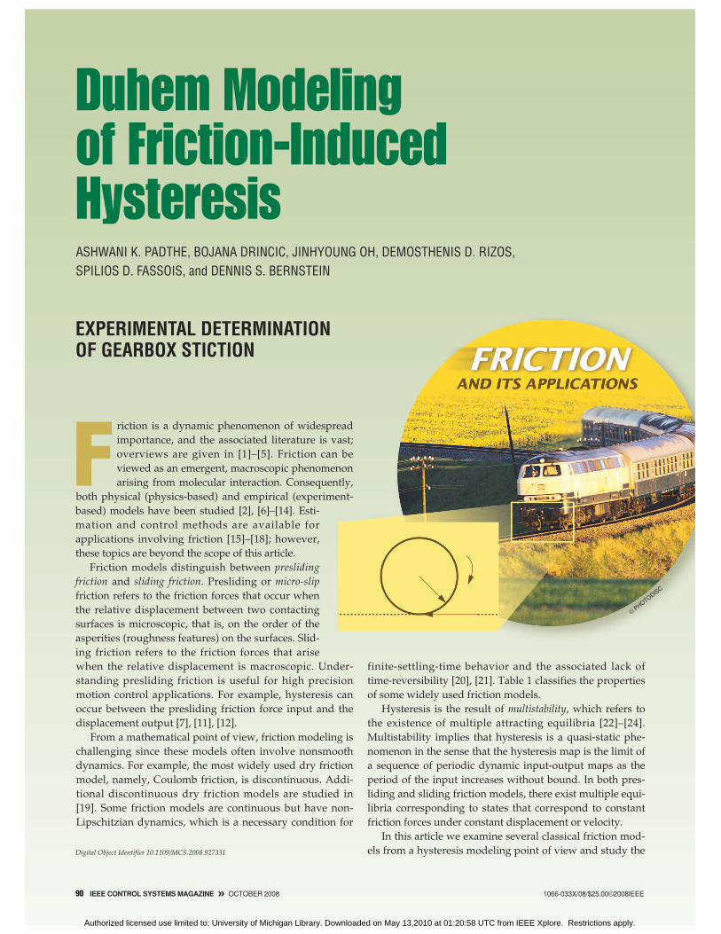
Friction is a dynamic phenomenon of widespreadimportance, and the associated literature is vast;overviews are given in [1]–[5]. Friction can beviewed as an emergent, macroscopic phenomenonarising from molecular interaction. Consequently,

both physical (physics-based) and empirical (experiment-based) models have been studied [2], [6]–[14]. Esti-mation and control methods are available forapplications involving friction [15]–[18]; however,these topics are beyond the scope of this article.

Friction models distinguish between preslidingfriction and sliding friction. Presliding or micro-slipfriction refers to the friction forces that occur whenthe relative displacement between two contactingsurfaces is microscopic, that is, on the order of theasperities (roughness features) on the surfaces. Slid-ing friction refers to the friction forces that arisewhen the relative displacement is macroscopic. Under-standing presliding friction is useful for high precisionmotion control applications. For example, hysteresis canoccur between the presliding friction force input and thedisplacement output [7], [11], [12].

From a mathematical point of view, friction modeling ischallenging since these models often involve nonsmoothdynamics. For example, the most widely used dry frictionmodel, namely, Coulomb friction, is discontinuous. Addi-tional discontinuous dry friction models are studied in[19]. Some friction models are continuous but have non-Lipschitzian dynamics, which is a necessary condition for

finite-settling-time behavior and the associated lack oftime-reversibility [20], [21]. Table 1 classifies the propertiesof some widely used friction models.

Hysteresis is the result of multistability, which refers tothe existence of multiple attracting equilibria [22]–[24].Multistability implies that hysteresis is a quasi-static phe-nomenon in the sense that the hysteresis map is the limit ofa sequence of periodic dynamic input-output maps as theperiod of the input increases without bound. In both pres-liding and sliding friction models, there exist multiple equi-libria corresponding to states that correspond to constantfriction forces under constant displacement or velocity.

In this article we examine several classical friction mod-els from a hysteresis modeling point of view and study the

Duhem Modeling of Friction-Induced HysteresisASHWANI K. PADTHE, BOJANA DRINCIC, JINHYOUNG OH, DEMOSTHENIS D. RIZOS, SPILIOS D. FASSOIS, and DENNIS S. BERNSTEIN

EXPERIMENTAL DETERMINATION OF GEARBOX STICTION

Digital Object Identifier 10.1109/MCS.2008.927331

©PHOTODIS

C

90 IEEE CONTROL SYSTEMS MAGAZINE » OCTOBER 2008 1066-033X/08/$25.00©2008IEEE

Authorized licensed use limited to: University of Michigan Library. Downloaded on May 13,2010 at 01:20:58 UTC from IEEE Xplore. Restrictions apply.

hysteresis induced by these friction models when incorpo-rated into a physical system. Our starting point is [25],which focuses on the Duhem model for hysteresis. Formore information on Duhem models, see [26]. The Duhemmodel has the property that, under constant inputs, everystate is an equilibrium. When there exist multiple attract-ing (step-convergent) equilibria for a given step input, thesystem exhibits hysteresis under inputs that drive the sys-tem through distinct equilibria that map into distinct out-puts. In certain cases, the limiting input-output map isindependent of the input period; this case is known as rate-independent hysteresis. In general, the hysteresis map is ratedependent, although the terminology is slightly misleadingsince, as already noted, hysteresis per se is a quasi-staticphenomenon.

The generalized Duhem model x = f (x, u)g (u) and itsspecialization x = (Ax + Bu)g (u), known as the semilinearDuhem model, are considered in [25]. These models giverise to rate-independent hysteresis when the function g ispositively homogeneous; otherwise, the hysteresis is gen-erally rate dependent.

In the present article we consider three friction models,namely, the Dahl, LuGre (Lund/Grenoble), and Maxwell-slipmodels. We recast each model in the form of a generalized orsemilinear Duhem model to provide a unified framework forcomparing the hysteretic nature of these models. For exam-ple, the Dahl model is shown to be a rate-independent gener-alized Duhem model. Furthermore, in one special case, theDahl model is also a semilinear Duhem model for which aclosed-form solution is available. Similarly, the LuGre modelis a rate-dependent generalized Duhem model. Next, weembed each friction model within a single-degree-of-freedommechanical model to examine and compare the hystereticresponse of the combined system.

Finally, we develop an experimental testbed for frictionidentification. The testbed consists of a dc motor with aspeed-reduction gearhead, encoder measurements of theshaft, tachometer measurements of the shaft angular veloc-ity, and load-cell tension measurements of a cable woundaround the drum. By operating this testbed under quasi-static conditions, we compare its hysteretic response to thesimulated response of the system under various friction

models. The goal is to identify a model for the friction andstiction effects observed in the testbed by comparing thesimulation and experimental results.

The objective of this article is to reformulate the Dahl,LuGre, and Maxwell-slip models as Duhem models tounderstand their hysteretic properties. This classificationprovides the framework for identifying a friction modelthat captures the hysteretic behavior of the motor gearbox.

The contents of the article are as follows. In the fol-lowing section we review the basic theory of the Duhemmodel. Next, we recast the Dahl, LuGre, and Maxwell-slip models as Duhem models and relate their dynamicbehavior to properties of the Duhem models. We thenstudy the sliding friction dynamics of the three frictionmodels. Next, we consider friction-induced hysteresis ina mass-spring system. This system is studied as a specialcase of a linear time-invariant system with Duhem feed-back. We then develop a model of the experimentalsetup and simulate the model using all three frictionmodels. We then report the experimental results andcompare them with the simulation results to obtain esti-mates of the friction parameters. Finally, we give someconcluding remarks.

GENERALIZED AND SEMILINEAR DUHEM MODELSIn this section, we summarize the main results of [25]concerning the generalized and semilinear Duhem mod-els. Consider the single-input, single-output generalizedDuhem model

x(t) = f (x(t), u(t))g(u(t)), x(0) = x0, t ≥ 0, (1)

y(t) = h(x(t), u(t)), (2)

where x : [0,∞) → Rn is absolutely continuous,u : [0,∞) → R is continuous and piecewise C1 ,f : Rn × R → Rn×r is continuous, g : R → Rr is continu-ous and satisfies g (0) = 0, and y : [0,∞) → R , andh : Rn × R → R are continuous. The value of x(t) at apoint t at which u(t) does not exist can be assigned arbi-trarily. We assume that the solution to (1) exists and isunique on all finite intervals. Under these assumptions, xand y are continuous and piecewise C1. The terms closed

OCTOBER 2008 « IEEE CONTROL SYSTEMS MAGAZINE 91

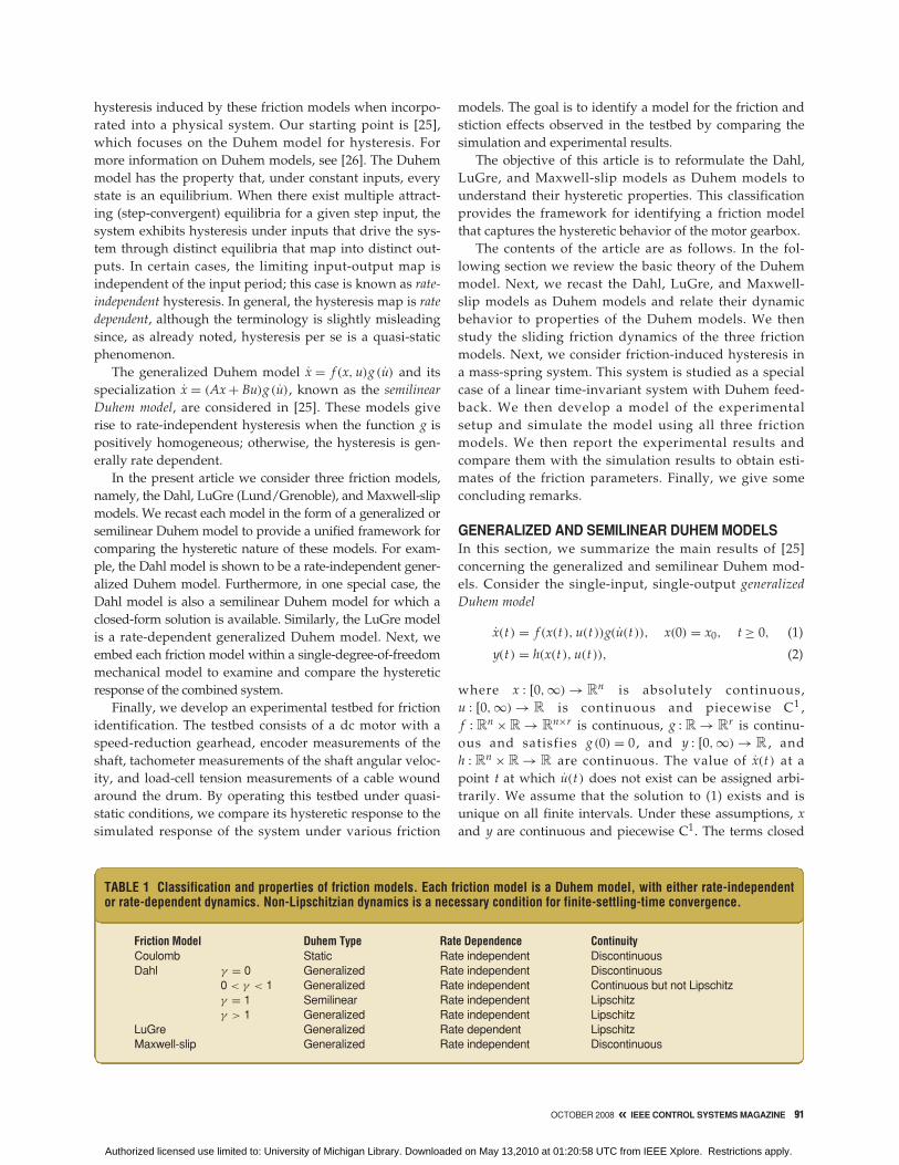
TABLE 1 Classification and properties of friction models. Each friction model is a Duhem model, with either rate-independentor rate-dependent dynamics. Non-Lipschitzian dynamics is a necessary condition for finite-settling-time convergence.

Friction Model Duhem Type Rate Dependence ContinuityCoulomb Static Rate independent DiscontinuousDahl γ = 0 Generalized Rate independent Discontinuous

0 < γ < 1 Generalized Rate independent Continuous but not Lipschitzγ = 1 Semilinear Rate independent Lipschitzγ > 1 Generalized Rate independent Lipschitz

LuGre Generalized Rate dependent LipschitzMaxwell-slip Generalized Rate independent Discontinuous


curve, limiting periodic input-output map, hysteresis map,and rate independence are defined as follows.

Definition 1The nonempty set H ⊂ R2 is a closed curve if there exists acontinuous, piecewise C1 , and periodic mapγ : [0,∞) → R2 such that γ ([0,∞)) = H.

Definition 2Let u : [0,∞) → [umin, umax] be continuous, piecewise C1,periodic with period α, and have exactly one local maxi-mum umax in [0, α) and exactly one local minimum umin in[0, α). For all T > 0, define uT(t) � u(αt/T ), assume thatthere exists xT : [0,∞) → Rn that is periodic with period Tand satisfies (1) with u = uT , and let yT : [0,∞) → R begiven by (2) with x = xT and u = uT . For all T > 0, the peri-odic input-output map HT (uT, yT, x0) is the closed curveHT(uT, yT, x0) � {(uT(t), yT(t)) : t ∈ [0,∞)}, and the limit-ing periodic input-output map H∞(u, x0) is the closedcurve H∞(u, x0) � limT→∞ HT (uT, yT, x0) if the limitexists. If there exist (u, y1), (u, y2) ∈ H∞(u, x0) such thaty1 �= y2, then H∞(u) is a hysteresis map, and the general-ized Duhem model is hysteretic. If, in addition H∞(u, x0)

is independent of x0 then the generalized Duhem modelhas local memory, and we write H∞(u) . Otherwise,H∞(u, x0) has nonlocal memory.

Definition 3The continuous and piecewise C1 function τ : [0,∞) → [0,∞)

is a positive time scale if τ(0) = 0, τ is nondecreasing, andlimt→∞ τ(t) = ∞. The generalized Duhem model (1), (2) israte independent if, for every pair of continuous and piece-wise C1 functions x and u satisfying (1) and for every posi-tive time scale τ , it follows that xτ (t) � x(τ(t)) anduτ (t) � u(τ(t)) also satisfy (1).

The following result is proved in [25].

Proposition 1Assume that g is positively homogeneous, that is,g (αv) = αg (v) for all α > 0 and v ∈ R. Then the general-ized Duhem model (1), (2) is rate independent.

If g is positively homogeneous, then there existh+, h− ∈ Rr such that

g (v) ={

h+v, v ≥ 0,

h−v, v < 0,(3)

and the rate-independent generalized Duhem model (1),(2) can be reparameterized in terms of u [25]. Specifically,consider

dx(u)

du=

⎧⎨⎩

f+(x(u), u), when u increases,f−(x(u), u), when u decreases,0, otherwise,

(4)

y(u) = h(x(u), u), (5)

for u ∈ [umin, umax] and with initial condition x(u0) = x0,where f+(x, u) � f (x, u)h+ , f−(x, u) � f (x, u)h− , andu0 ∈ [umin, umax] . Then x(t) � x(u(t)) and y(t) � y(u(t))satisfy (1), (2). Note that the reparameterized Duhemmodel (4) and (5) can be viewed as a time-varying dynami-cal system with nonmonotonic time u.

As a specialization of (1) and (2), we now consider therate-independent semilinear Duhem model

x(t) = [ u+(t)In u−(t)In ]

×([

A+A−

]x(t) +

[B+B−

]u(t) +

[E+E−

]), (6)

y(t) = Cx(t) + Du(t), x(0) = x0, t ≥ 0, (7)

where A+ ∈ Rn×n , A− ∈ Rn×n , B+ ∈ Rn , B− ∈ Rn ,E+ ∈ Rn, E− ∈ Rn, C ∈ R1×n, D ∈ R, and

u+(t) � max{0, u(t)}, u−(t) � min{0, u(t)}. (8)

Let ρ(A) denote the spectral radius of A ∈ Rn×n and letthe limiting input-output map F∞(u, y) be the set of pointsz ∈ R2 such that there exists an increasing, divergentsequence {ti}∞i=1 in [0,∞) satisfying

limi→∞

‖(u(ti), y(ti)) − z‖ = 0.

The following result given in [25] provides a sufficient con-dition for the existence of the limiting periodic input-outputmap for the rate-independent semilinear Duhem model.

Theorem 1Consider the rate-independent semilinear Duhem model (6),(7), where u : [0,∞) → [umin, umax] is continuous, piecewiseC1, and periodic with period α and has exactly one local maxi-mum umax in [0, α) and exactly one local minimum umin in[0, α). Furthermore, define β � umax − umin, and assume that

ρ(eβA+ e−βA−) < 1. (9)

Then, for all x0 ∈ Rn , (6) has a unique periodic solutionx : [0,∞) → Rn , and the limiting periodic input-outputmap H∞(u, x0) exists. Specifically, if A+ and A− are invert-ible, then

H∞(u) = {(u, y+(u)) ∈ R2 : u ∈ [umin, umax]}

∪ {(u, y−(u)) ∈ R2 : u ∈ [umin, umax]}, (10)

where

y+(u) = CeA+(u−umin)x+ − CZ+(u, umin) + Du,

y−(u) = CeA−(u−umax)x− − CZ−(u, umax) + Du,

and

92 IEEE CONTROL SYSTEMS MAGAZINE » OCTOBER 2008


x+ � −(I − e−βA− eβA+)−1(e−βA−Z+(umax, umin)

+ Z−(umin, umax)),

x− � −(I − eβA+ e−βA−)−1(eβA+Z−(umin, umax)

+ Z+(umax, umin)),

Z+(u, u0) � A−1+ (uI − u0eA+(u−u0))B+

+ A−2+ (I − eA+(u−u0))B+ + A−1

+ (I − eA+(u−u0))E+,

Z−(u, u0) � A−1− (uI − u0eA−(u−u0))B−

+ A−2− (I − eA−(u−u0))B− + A−1

− (I − eA−(u−u0))E−.

See [25] for the case in which A+ or A− is singular.Definition 2 and Theorem 1 imply that the rate-inde-

pendent semilinear Duhem model has local memory sincethe hysteresis map H∞(u) given by (10) is independent ofthe initial condition x0 ∈ Rn.

FRICTION MODELS

Dahl ModelThe Dahl model [6], [27], [28] has the form

F (t) = σ

∣∣∣∣1 − F(t)FC

sgn u(t)∣∣∣∣γ sgn

(1 − F(t)

FCsgn u(t)

)u(t),

(11)

where F is the friction force, u is the relative displacementbetween the two surfaces in contact, FC > 0 is theCoulomb friction force, γ ≥ 0 is a parameter that deter-mines the shape of the force-deflection curve (as represent-ed by a plot of the friction force versus the relativedisplacement), and σ > 0 is the rest stiffness, that is, theslope of the force-deflection curve when F = 0. The right-hand side of (11) is Lipschitz continuous in F for γ ≥ 1 butnot Lipschitz continuous in F for 0 ≤ γ < 1.

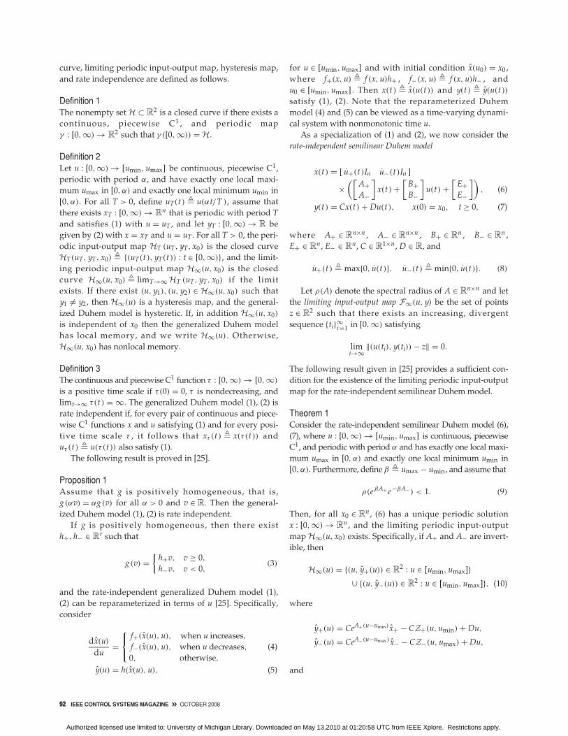
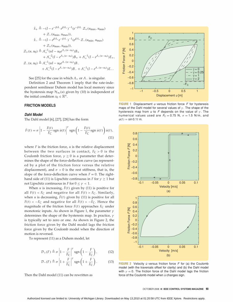
When u is increasing, F(t) given by (11) is positive forall F(t) < FC and negative for all F(t) > FC . Similarly,when u is decreasing, F(t) given by (11) is positive for allF(t) < −FC and negative for all F(t) > −FC . Hence themagnitude of the friction force F(t) approaches FC undermonotonic inputs. As shown in Figure 1, the parameter γdetermines the shape of the hysteresis map. In practice, γis typically set to zero or one. As shown in Figure 2, thefriction force given by the Dahl model lags the frictionforce given by the Coulomb model when the direction ofmotion is reversed.

To represent (11) as a Duhem model, let

D+(F ) � σ

∣∣∣∣1 − FFC

∣∣∣∣γ sgn(

1 − FFC

), (12)

D−(F ) � σ

∣∣∣∣1 + FFC

∣∣∣∣γ sgn(

1 + FFC

). (13)

Then the Dahl model (11) can be rewritten as

FIGURE 1 Displacement u versus friction force F for hysteresismaps of the Dahl model for several values of γ . The shape of thehysteresis map from u to F depends on the value of γ . Thenumerical values used are FC = 0.75 N, σ = 1.5 N/m, andu(t ) = sin 0.1t m.

−1 −0.5 0 0.5 1−1

−0.8

−0.6

−0.4

−0.2

0

0.2

0.4

0.6

0.8

1

Displacement u [m]

Fric

tion

For

ce F

[N]

FC

−FC

γ = 0γ = 0.25γ = 1γ = 2

FIGURE 2 Velocity u versus friction force F for (a) the Coulombmodel (with the traversals offset for clarity) and (b) the Dahl modelwith γ = 0. The friction force of the Dahl model lags the frictionforce of the Coulomb model when u changes sign.

−0.1 −0.05 0 0.05 0.1−0.8

−0.6

−0.4

−0.2

0

0.2

0.4

0.6

0.8

Fric

tion

For

ce F

[N]

Velocity [m/s]

(a)

−0.1 −0.05 0 0.05 0.1

−1

00.20.40.60.8

1

Fric

tion

For

ce F

[N]

−0.6−0.8

−0.4−0.2

Velocity [m/s]

(b)



F(t) = σ [D+(F(t)) D−(F(t)) ]

×[

u+(t)u−(t)

], (14)

y = F, (15)

which, for all γ ≥ 0, is a generalized Duhem model of theform (1), (2). Furthermore, since g(u) = [ u+(t) u−(t) ]T ispositively homogeneous, Proposition 1 implies that (14) israte independent for all γ ≥ 0.

Let γ = 1. Then (11) becomes

F (t) = σ

(1 − F (t)

FCsgn u(t)

)u(t)

=[− σ

FCF (t) + σ σ

FCF (t) + σ

] [u+(t)u−(t)

],

which is a rate-independent semilinear Duhem model.Furthermore, the convergence condition (9) becomes

e−2 βσ

FC < 1, (16)

which holds if and only if β > 0. As a direct consequenceof Theorem 1, which explicitly characterizes the hysteresismap, we have the following result. The corresponding hys-teresis map is shown in Figure 1.

Corollary 1Consider the Dahl model (11) with γ = 1. Letu : [0,∞) → [umin, umax] be continuous, piecewise C1, andperiodic with period α and have exactly one local maxi-mum umax in [0, α) and exactly one local minimum umin in

[0, α). Then (16) holds, and (14), (15) has a unique periodicsolution F : [0,∞) → Rn , and, for all x0 ∈ Rn, the limitingperiodic input-output map H∞(u) exists. Furthermore,

H∞(u) ={(u, F+(u)) ∈ R

2 : u ∈ [umin, umax]}

∪{(u, F−(u)) ∈ R

2 : u ∈ [umin, umax]}

, (17)

where

F+(u) � e− σFC

(u−umin)α+ + FC

(1 − e− σ

FC(u−umin)

),

F−(u) � eσ

FC(u−umax)

α− − FC

(1 − e− σ

FC(u−umax)

),

and

α+ = −α− = FCe

−βσ

FC − 1

e−βσ

FC + 1.

Corollary 1 implies that the Dahl model (11) with γ = 1 haslocal memory since it is a rate-independent semilinear Duhemmodel and H∞(u) defined by (17) is independent of x0.

LuGre ModelThe LuGre model [10], which models the asperities of twosurfaces as elastic bristles, is given by

x(t) = u(t) − |u(t)|r(u(t))

x(t), (18)

F(t) = σ0x(t) + σ1x(t) + σ2u(t), (19)

where x is the average deflection of the bristles, u is the rel-ative displacement, F is the friction force, and σ0, σ1, σ2 > 0are stiffness, damping, and viscous friction coefficients,respectively. The right-hand side of (18) is Lipschitz contin-uous with respect to x. In [1] and [10], r(u(t)) is defined by

r(u(t)) = FC

σ0+ FS − FC

σ0e−(u(t)/vS)

2, (20)

where FC > 0 is the Coulomb friction force, FS is the stic-tion (sticking friction) force, and vS is the Stribeck velocity.

For a given constant velocity u, the steady-state frictionforce Fss obtained from (18) and (19) is

Fss(u) = σ0r(u)sgn(u) + σ2u . (21)

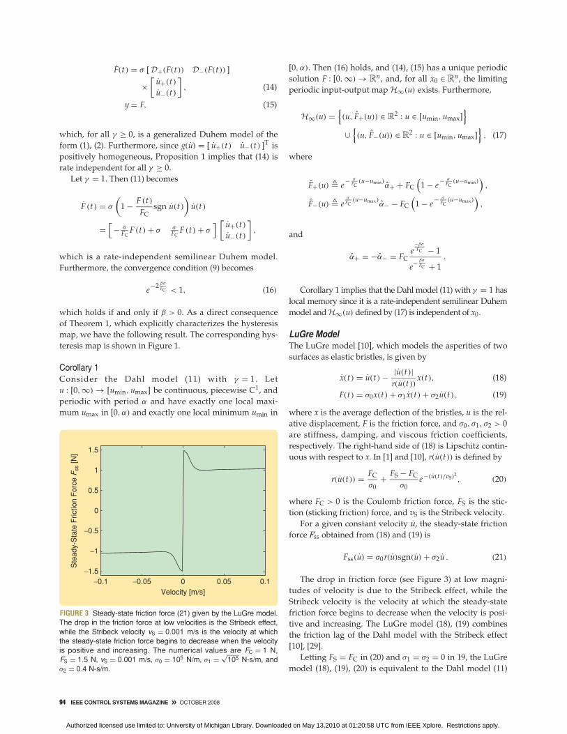
The drop in friction force (see Figure 3) at low magni-tudes of velocity is due to the Stribeck effect, while theStribeck velocity is the velocity at which the steady-statefriction force begins to decrease when the velocity is posi-tive and increasing. The LuGre model (18), (19) combinesthe friction lag of the Dahl model with the Stribeck effect[10], [29].

Letting FS = FC in (20) and σ1 = σ2 = 0 in 19, the LuGremodel (18), (19), (20) is equivalent to the Dahl model (11)

FIGURE 3 Steady-state friction force (21) given by the LuGre model.The drop in the friction force at low velocities is the Stribeck effect,while the Stribeck velocity vS = 0.001 m/s is the velocity at whichthe steady-state friction force begins to decrease when the velocityis positive and increasing. The numerical values are FC = 1 N,FS = 1.5 N, vS = 0.001 m/s, σ0 = 105 N/m, σ1 = √

105 N-s/m, andσ2 = 0.4 N-s/m.

−0.1 −0.05 0 0.05 0.1−1.5

−1

−0.5

0

0.5

1

1.5

Velocity [m/s]

Ste

ady-

Sta

te F

rictio

n F

orce

Fss

[N]



with γ = 1 and σ = 1. With y = F, the state equations (18)and (19) can be written as

x(t) = [ 1 x(t) ][

u(t)− |u(t)|

r(u(t))

], (22)

y(t) = σ0x(t) + σ1x(t) + σ2u(t), (23)

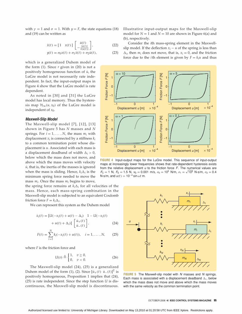
which is a generalized Duhem model ofthe form (1). Since r given in (20) is not apositively homogeneous function of u, theLuGre model is not necessarily rate inde-pendent. In fact, the input-output maps inFigure 4 show that the LuGre model is ratedependent.

As noted in [30] and [31] the LuGremodel has local memory. Thus the hystere-sis map H∞(u, x0) of the LuGre model isindependent of x0.

Maxwell-Slip ModelThe Maxwell-slip model [7], [12], [13]shown in Figure 5 has N masses and Nsprings. For i = 1, . . . , N, the mass mi withdisplacement xi is connected by a stiffness kito a common termination point whose dis-placement is u. Associated with each mass isa displacement deadband of width �i > 0,below which the mass does not move, andabove which the mass moves with velocityu, that is, the inertia of the masses is ignoredwhen the mass is sliding. Hence, ki�i is theminimum spring force needed to move themass mi. Once the mass mi begins to move,the spring force remains at ki�i for all velocities of themass. Hence, each mass-spring combination in theMaxwell-slip model is subjected to an equivalent Coulombfriction force F = ki�i.

We can represent this system as the Duhem model

xi(t) = [U(−xi(t) + u(t) − �i) 1 − U(−xi(t)

+ u(t) + �i)][

u+(t)u−(t)

], (24)

F(t) =N∑

i=1

ki(−xi(t) + u(t)), i = 1, . . . , N, (25)

where F is the friction force and

U(v) �{

1, v ≥ 0,

0, v < 0.(26)

The Maxwell-slip model (24), (25) is a generalizedDuhem model of the form (1), (2). Since [u+(t) u−(t)]T ispositively homogeneous, Proposition 1 implies that (24),(25) is rate independent. Since the step function U is dis-continuous, the Maxwell-slip model is discontinuous.

Illustrative input-output maps for the Maxwell-slipmodel for N = 1 and N = 10 are shown in Figure 6(a) and(b), respectively.

Consider the ith mass-spring element in the Maxwell-slip model. If the deflection xi − u of the spring is less than�i, then mi does not move, that is, xi = 0, and the frictionforce due to the i th element is given by F = kiu and thus

FIGURE 4 Input-output maps for the LuGre model. This sequence of input-outputmaps at increasingly lower frequencies shows that rate-dependent hysteresis existsfrom the relative displacement u to the friction force F . The numerical values areFC = 1 N, FS = 1.5 N, vS = 0.001 m/s, σ0 = 105 N/m, σ1 = √

105 N-s/m, σ2 = 0.4N-s/m, and u(t ) = 10−4 sin ωt m.

−1 0 1

−1

0

1

Fric

tion

For

ce F

[N] ω = 10

−1 0 1

−1

0

1

Fric

tion

For

ce F

[N]

Fric

tion

For

ce F

[N]

ω = 5

−1 0 1

−1

0

1

Fric

tion

For

ce F

[N] ω = 1

−1 0 1

−1

0

1

ω = 0.1

Displacement u [m] × 10−4

Displacement u [m]

Displacement u [m] Displacement u [m]

× 10−4

× 10−4 × 10

−4

FIGURE 5 The Maxwell-slip model with N masses and N springs.Each mass is associated with a displacement deadband �i , belowwhich the mass does not move and above which the mass moveswith the same velocity as the common termination point.

u

x1

m1 Δ1

k1

xi

xN

mi

mN

Δi

ΔN

ki

kN



F = kiu. If the deflection is equal to �i, then xi = u, andhence F = ki�i and thus F = 0. Consequently, each mass-spring combination in the Maxwell-slip model is a Dahlmodel with γ = 0 and σ = ki, which has the form

F(t) = ki

[sgn

(1 − F(t)

FCsgn u(t)

)]u(t).

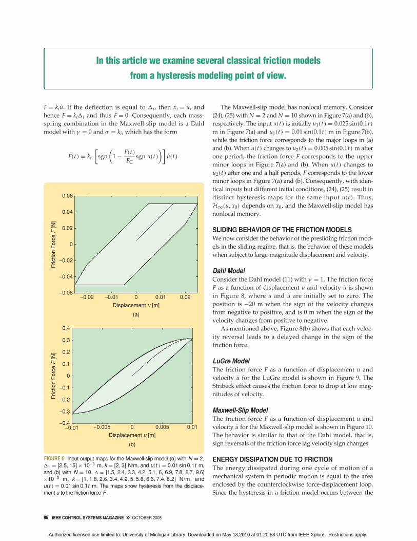
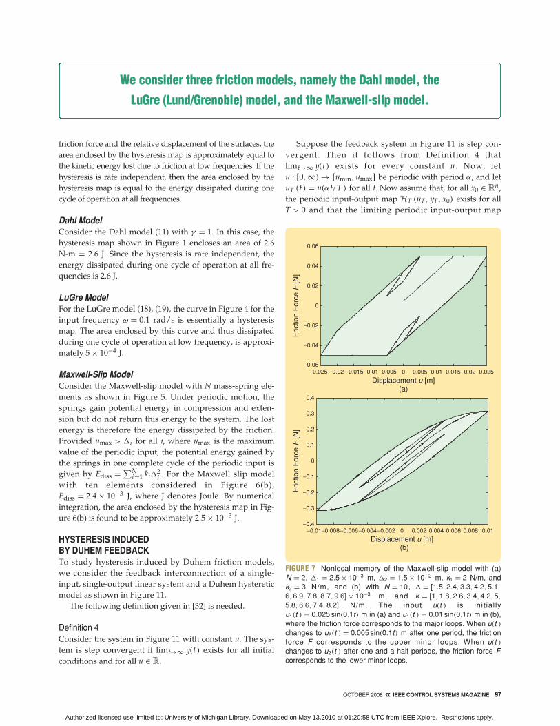
The Maxwell-slip model has nonlocal memory. Consider(24), (25) with N = 2 and N = 10 shown in Figure 7(a) and (b),respectively. The input u(t) is initially u1(t) = 0.025 sin(0.1t)m in Figure 7(a) and u1(t) = 0.01 sin(0.1t) m in Figure 7(b),while the friction force corresponds to the major loops in (a)and (b). When u(t) changes to u2(t) = 0.005 sin(0.1t) m afterone period, the friction force F corresponds to the upperminor loops in Figure 7(a) and (b). When u(t) changes tou2(t) after one and a half periods, F corresponds to the lowerminor loops in Figure 7(a) and (b). Consequently, with iden-tical inputs but different initial conditions, (24), (25) result indistinct hysteresis maps for the same input u(t). Thus,H∞(u, x0) depends on x0, and the Maxwell-slip model hasnonlocal memory.

SLIDING BEHAVIOR OF THE FRICTION MODELSWe now consider the behavior of the presliding friction mod-els in the sliding regime, that is, the behavior of these modelswhen subject to large-magnitude displacement and velocity.

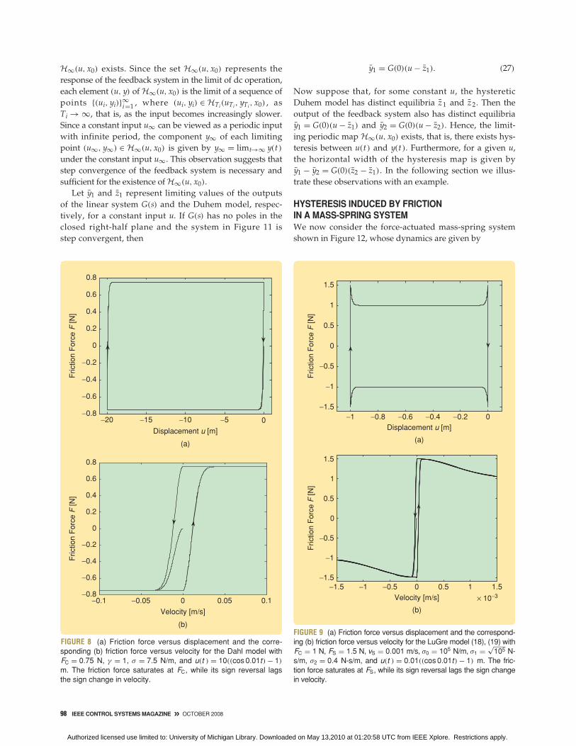
Dahl ModelConsider the Dahl model (11) with γ = 1. The friction forceF as a function of displacement u and velocity u is shownin Figure 8, where u and u are initially set to zero. Theposition is −20 m when the sign of the velocity changesfrom negative to positive, and is 0 m when the sign of thevelocity changes from positive to negative.

As mentioned above, Figure 8(b) shows that each veloc-ity reversal leads to a delayed change in the sign of thefriction force.

LuGre ModelThe friction force F as a function of displacement u andvelocity u for the LuGre model is shown in Figure 9. TheStribeck effect causes the friction force to drop at low mag-nitudes of velocity.

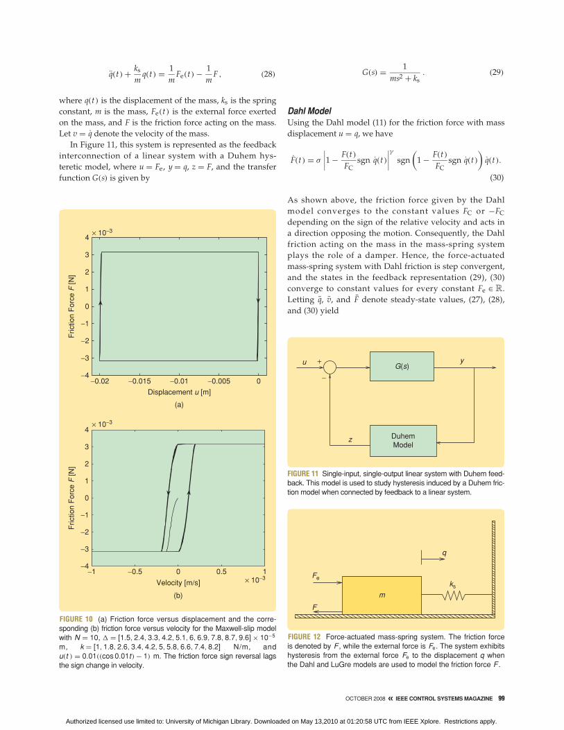
Maxwell-Slip ModelThe friction force F as a function of displacement u andvelocity u for the Maxwell-slip model is shown in Figure 10.The behavior is similar to that of the Dahl model, that is,sign reversals of the friction force lag velocity sign changes.

ENERGY DISSIPATION DUE TO FRICTIONThe energy dissipated during one cycle of motion of amechanical system in periodic motion is equal to the areaenclosed by the counterclockwise force-displacement loop.Since the hysteresis in a friction model occurs between the

FIGURE 6 Input-output maps for the Maxwell-slip model (a) with N = 2,�1 = [2.5, 15] × 10−3 m, k = [2, 3] N/m, and u(t ) = 0.01 sin 0.1t m,and (b) with N = 10, � = [1.5, 2.4, 3.3, 4.2, 5.1, 6, 6.9, 7.8, 8.7, 9.6]×10−3 m, k = [1, 1.8, 2.6, 3.4, 4.2, 5, 5.8, 6.6, 7.4, 8.2] N/m, andu(t ) = 0.01 sin 0.1t m. The maps show hysteresis from the displace-ment u to the friction force F .

−0.02 −0.01 0 0.01 0.02−0.06

−0.04

−0.02

0

0.02

0.04

0.06

Displacement u [m]

Fric

tion

For

ce F

[N]

(a)

−0.01 −0.005 0 0.005 0.01−0.4

−0.3

−0.2

−0.1

0

0.1

0.2

0.3

0.4

Displacement u [m]

Fric

tion

For

ce F

[N]

(b)


In this article we examine several classical friction models

from a hysteresis modeling point of view.


friction force and the relative displacement of the surfaces, thearea enclosed by the hysteresis map is approximately equal tothe kinetic energy lost due to friction at low frequencies. If thehysteresis is rate independent, then the area enclosed by thehysteresis map is equal to the energy dissipated during onecycle of operation at all frequencies.

Dahl ModelConsider the Dahl model (11) with γ = 1. In this case, thehysteresis map shown in Figure 1 encloses an area of 2.6N-m = 2.6 J. Since the hysteresis is rate independent, theenergy dissipated during one cycle of operation at all fre-quencies is 2.6 J.

LuGre ModelFor the LuGre model (18), (19), the curve in Figure 4 for theinput frequency ω = 0.1 rad/s is essentially a hysteresismap. The area enclosed by this curve and thus dissipatedduring one cycle of operation at low frequency, is approxi-mately 5 × 10−4 J.

Maxwell-Slip ModelConsider the Maxwell-slip model with N mass-spring ele-ments as shown in Figure 5. Under periodic motion, thesprings gain potential energy in compression and exten-sion but do not return this energy to the system. The lostenergy is therefore the energy dissipated by the friction.Provided umax > �i for all i, where umax is the maximumvalue of the periodic input, the potential energy gained bythe springs in one complete cycle of the periodic input isgiven by Ediss = ∑N

i=1 ki�2i . For the Maxwell slip model

with ten elements considered in Figure 6(b),Ediss = 2.4 × 10−3 J, where J denotes Joule. By numericalintegration, the area enclosed by the hysteresis map in Fig-ure 6(b) is found to be approximately 2.5 × 10−3 J.

HYSTERESIS INDUCEDBY DUHEM FEEDBACKTo study hysteresis induced by Duhem friction models,we consider the feedback interconnection of a single-input, single-output linear system and a Duhem hystereticmodel as shown in Figure 11.

The following definition given in [32] is needed.

Definition 4Consider the system in Figure 11 with constant u. The sys-tem is step convergent if limt→∞ y(t) exists for all initialconditions and for all u ∈ R.

Suppose the feedback system in Figure 11 is step con-vergent. Then it follows from Definition 4 thatlimt→∞ y(t) exists for every constant u. Now, letu : [0,∞) → [umin, umax] be periodic with period α, and letuT (t) = u(αt/T ) for all t. Now assume that, for all x0 ∈ Rn,the periodic input-output map HT (uT, yT, x0) exists for allT > 0 and that the limiting periodic input-output map

FIGURE 7 Nonlocal memory of the Maxwell-slip model with (a)N = 2, �1 = 2.5 × 10−3 m, �2 = 1.5 × 10−2 m, k1 = 2 N/m, andk2 = 3 N/m, and (b) with N = 10, � = [1.5, 2.4, 3.3, 4.2, 5.1,

6, 6.9, 7.8, 8.7, 9.6] × 10−3 m, and k = [1, 1.8, 2.6, 3.4, 4.2, 5,

5.8, 6.6, 7.4, 8.2] N/m. The input u(t ) is init ial lyu1(t ) = 0.025 sin(0.1t) m in (a) and u1(t ) = 0.01 sin(0.1t) m in (b),where the friction force corresponds to the major loops. When u(t )

changes to u2(t ) = 0.005 sin(0.1t) m after one period, the frictionforce F corresponds to the upper minor loops. When u(t )

changes to u2(t ) after one and a half periods, the friction force Fcorresponds to the lower minor loops.

−0.06

−0.04

−0.02

0

0.02

0.04

0.06

Displacement u [m]

Fric

tion

For

ce F

[N]

−0.025 −0.02 −0.015−0.01 0 0.005 0.01 0.015 0.02 0.025−0.005

(a)

−0.01−0.008−0.006−0.004−0.002 0 0.002 0.004 0.006 0.008 0.01−0.4

−0.3

−0.2

−0.1

0

0.1

0.2

0.3

0.4

Displacement u [m]

Fric

tion

For

ce F

[N]

(b)

We consider three friction models, namely the Dahl model, the

LuGre (Lund/Grenoble) model, and the Maxwell-slip model.



H∞(u, x0) exists. Since the set H∞(u, x0) represents theresponse of the feedback system in the limit of dc operation,each element (u, y) of H∞(u, x0) is the limit of a sequence ofpoints {(ui, yi)}∞i=1 , where (ui, yi) ∈ HTi(uTi, yTi, x0) , asTi → ∞, that is, as the input becomes increasingly slower.Since a constant input u∞ can be viewed as a periodic inputwith infinite period, the component y∞ of each limitingpoint (u∞, y∞) ∈ H∞(u, x0) is given by y∞ = limt→∞ y(t)under the constant input u∞. This observation suggests thatstep convergence of the feedback system is necessary andsufficient for the existence of H∞(u, x0).

Let y1 and z1 represent limiting values of the outputsof the linear system G(s) and the Duhem model, respec-tively, for a constant input u. If G(s) has no poles in theclosed right-half plane and the system in Figure 11 isstep convergent, then

y1 = G(0)(u − z1). (27)

Now suppose that, for some constant u, the hystereticDuhem model has distinct equilibria z1 and z2. Then theoutput of the feedback system also has distinct equilibriay1 = G(0)(u − z1) and y2 = G(0)(u − z2). Hence, the limit-ing periodic map H∞(u, x0) exists, that is, there exists hys-teresis between u(t) and y(t). Furthermore, for a given u,the horizontal width of the hysteresis map is given byy1 − y2 = G(0)(z2 − z1). In the following section we illus-trate these observations with an example.

HYSTERESIS INDUCED BY FRICTION IN A MASS-SPRING SYSTEMWe now consider the force-actuated mass-spring systemshown in Figure 12, whose dynamics are given by

FIGURE 8 (a) Friction force versus displacement and the corre-sponding (b) friction force versus velocity for the Dahl model withFC = 0.75 N, γ = 1, σ = 7.5 N/m, and u(t ) = 10((cos 0.01t) − 1)

m. The friction force saturates at FC, while its sign reversal lagsthe sign change in velocity.

−20 −15 −10 −5 0−0.8

−0.6

−0.4

−0.2

0

0.2

0.4

0.6

0.8

Displacement u [m]

Fric

tion

For

ce F

[N]

(a)

−0.1 −0.05 0 0.05 0.1−0.8

−0.6

−0.4

−0.2

0

0.2

0.4

0.6

0.8

Velocity [m/s]

Fric

tion

For

ce F

[N]

(b)FIGURE 9 (a) Friction force versus displacement and the correspond-ing (b) friction force versus velocity for the LuGre model (18), (19) withFC = 1 N, FS = 1.5 N, vS = 0.001 m/s, σ0 = 105 N/m, σ1 = √

105 N-s/m, σ2 = 0.4 N-s/m, and u(t ) = 0.01((cos 0.01t) − 1) m. The fric-tion force saturates at FS, while its sign reversal lags the sign changein velocity.

−1 −0.8 −0.6 −0.4 −0.2 0−1.5

−1

−0.5

0

0.5

1

1.5

Displacement u [m]

Fric

tion

For

ce F

[N]

(a)

−1.5 −1 −0.5 0 0.5 1 1.5

× 10−3

−1.5

−1

−0.5

0

0.5

1

1.5

Velocity [m/s]

Fric

tion

For

ce F

[N]

(b)



q(t) + ks

mq(t) = 1

mFe(t) − 1

mF , (28)

where q(t) is the displacement of the mass, ks is the springconstant, m is the mass, Fe(t) is the external force exertedon the mass, and F is the friction force acting on the mass.Let v = q denote the velocity of the mass.

In Figure 11, this system is represented as the feedbackinterconnection of a linear system with a Duhem hys-teretic model, where u = Fe, y = q, z = F, and the transferfunction G(s) is given by

G(s) = 1ms2 + ks

. (29)

Dahl ModelUsing the Dahl model (11) for the friction force with massdisplacement u = q, we have

F(t) = σ

∣∣∣∣1 − F(t)FC

sgn q(t)∣∣∣∣γ sgn

(1 − F(t)

FCsgn q(t)

)q(t).

(30)

As shown above, the friction force given by the Dahlmodel converges to the constant values FC or −FCdepending on the sign of the relative velocity and acts ina direction opposing the motion. Consequently, the Dahlfriction acting on the mass in the mass-spring systemplays the role of a damper. Hence, the force-actuatedmass-spring system with Dahl friction is step convergent,and the states in the feedback representation (29), (30)converge to constant values for every constant Fe ∈ R.Letting q, v, and F denote steady-state values, (27), (28),and (30) yield

FIGURE 10 (a) Friction force versus displacement and the corre-sponding (b) friction force versus velocity for the Maxwell-slip modelwith N = 10, � = [1.5, 2.4, 3.3, 4.2, 5.1, 6, 6.9, 7.8, 8.7, 9.6] × 10−5

m, k = [1, 1.8, 2.6, 3.4, 4.2, 5, 5.8, 6.6, 7.4, 8.2] N/m, andu(t ) = 0.01((cos 0.01t) − 1) m. The friction force sign reversal lagsthe sign change in velocity.

−0.02 −0.015 −0.01 −0.005 0−4

−3

−2

−1

0

1

2

3

4× 10−3

Displacement u [m]

Fric

tion

For

ce F

[N]

(a)

−1 −0.5 0 0.5 1

Velocity [m/s]

−4

−3

−2

−1

0

1

2

3

4

Fric

tion

For

ce F

[N]

× 10−3

× 10−3

(b)

FIGURE 11 Single-input, single-output linear system with Duhem feed-back. This model is used to study hysteresis induced by a Duhem fric-tion model when connected by feedback to a linear system.

G(s)

DuhemModel

u y

z

+

−

FIGURE 12 Force-actuated mass-spring system. The friction forceis denoted by F , while the external force is Fe. The system exhibitshysteresis from the external force Fe to the displacement q whenthe Dahl and LuGre models are used to model the friction force F .

F

Fe

m

q

ks



v = 0, (31)

q = G(0)(u − z) = Fe − Fks

, (32)(1 − F

FCsgn v

)= 0. (33)

For a constant external force input, the steady-state values ofdisplacement, velocity, and friction force are given by (31),(32), and (33), respectively. Thus, for a low-frequency exter-nal force input, v(t) → 0 as t → ∞, and the displacement ofthe mass satisfies q(t) → q as t → ∞, where q is given by(32). Now, if (33) holds, then F = FC or F = −FC dependingon the sign of v(t). Consequently, from (32), the steady-statedisplacement q can assume two different values, namely,

q1 = G(0)(Fe + FC) = Fe + FC

ks,

q2 = G(0)(Fe − FC) = Fe − FC

ks.

These observations suggest that the limit of the periodicmap HT (FeT, qT ) exists as T → ∞, that is, there exists hys-teresis between Fe(t) and q(t). The width of the map isgiven by q1 − q2 = 2Fc/ks . For ks = 1.5 N/m, Fc = 0.75 N,

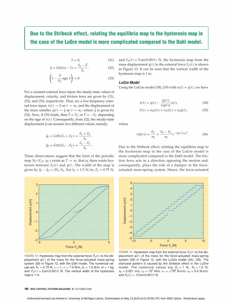
and Fe(t) = 5 sin(0.001t) N, the hysteresis map from themass displacement q(t) to the external force Fe(t) is shownin Figure 13. It can be seen that the vertical width of thehysteresis map is 1 m.

LuGre ModelUsing the LuGre model (18), (19) with u(t) = q(t), we have

x(t) = q(t) − |q(t)|r(q(t))

x(t), (34)

F(t) = σ0x(t) + σ1x(t) + σ2 q(t), (35)

where

r(q(t)) = FC

σ0+ FS − FC

σ0e−(q(t)/vS)

2. (36)

Due to the Stribeck effect, relating the equilibria map tothe hysteresis map in the case of the LuGre model ismore complicated compared to the Dahl model. The fric-tion force acts in a direction opposing the motion and,consequently, plays the role of a damper in the force-actuated mass-spring system. Hence, the force-actuated


FIGURE 13 Hysteresis map from the external force Fe(t ) to the dis-placement q(t ) of the mass for the force-actuated mass-springsystem (28) in Figure 12, with the Dahl model. The numerical val-ues are FC = 0.75 N, γ = 1, σ = 7.5 N/m, ks = 1.5 N/m, m = 1 kg,and Fe(t ) = 5 sin(0.001t) N. The vertical width of the hysteresismap is 1 m.

−5 0 5−3

−2

−1

0

1

2

3

Dis

plac

emen

t q [m

]

Force Fe [N]

FIGURE 14 Hysteresis map from the external force Fe(t ) to the dis-placement q(t ) of the mass for the force-actuated mass-springsystem (28) in Figure 12, with the LuGre model (34), (35). Thestaircase pattern is caused by the Stribeck effect in the LuGremodel. The numerical values are FC = 1 N, FS = 1.5 N,vS = 0.001 m/s, σ0 = 105 N/m, σ1 = √

105 N-s/m, σ2 = 0.4 N-s/m,and Fe(t ) = 10 sin(0.001t) N.

−10 −5 0 5 10−5

−4

−3

−2

−1

0

1

2

3

4

5

Dis

plac

emen

t q [m

]

Force Fe [N]

Due to the Stribeck effect, relating the equilibria map to the hysteresis map in

the case of the LuGre model is more complicated compared to the Dahl model.


mass-spring system with LuGre friction is step conver-gent, and the states in the feedback representation givenby (29), (34), and (35) converge to constant values forevery constant Fe ∈ R.

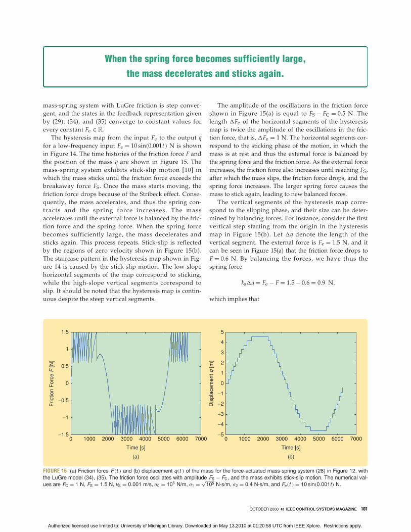
The hysteresis map from the input Fe to the output qfor a low-frequency input Fe = 10 sin(0.001t) N is shownin Figure 14. The time histories of the friction force F andthe position of the mass q are shown in Figure 15. Themass-spring system exhibits stick-slip motion [10] inwhich the mass sticks until the friction force exceeds thebreakaway force FS. Once the mass starts moving, thefriction force drops because of the Stribeck effect. Conse-quently, the mass accelerates, and thus the spring con-tracts and the spring force increases. The massaccelerates until the external force is balanced by the fric-tion force and the spring force. When the spring forcebecomes sufficiently large, the mass decelerates andsticks again. This process repeats. Stick-slip is reflectedby the regions of zero velocity shown in Figure 15(b).The staircase pattern in the hysteresis map shown in Fig-ure 14 is caused by the stick-slip motion. The low-slopehorizontal segments of the map correspond to sticking,while the high-slope vertical segments correspond toslip. It should be noted that the hysteresis map is contin-uous despite the steep vertical segments.

The amplitude of the oscillations in the friction forceshown in Figure 15(a) is equal to FS − FC = 0.5 N. Thelength �Fe of the horizontal segments of the hysteresismap is twice the amplitude of the oscillations in the fric-tion force, that is, �Fe = 1 N. The horizontal segments cor-respond to the sticking phase of the motion, in which themass is at rest and thus the external force is balanced bythe spring force and the friction force. As the external forceincreases, the friction force also increases until reaching FS,after which the mass slips, the friction force drops, and thespring force increases. The larger spring force causes themass to stick again, leading to new balanced forces.

The vertical segments of the hysteresis map corre-spond to the slipping phase, and their size can be deter-mined by balancing forces. For instance, consider the firstvertical step starting from the origin in the hysteresismap in Figure 15(b). Let �q denote the length of thevertical segment. The external force is Fe = 1.5 N, and itcan be seen in Figure 15(a) that the friction force drops toF = 0.6 N. By balancing the forces, we have thus thespring force

ks�q = Fe − F = 1.5 − 0.6 = 0.9 N,

which implies that


FIGURE 15 (a) Friction force F(t ) and (b) displacement q(t ) of the mass for the force-actuated mass-spring system (28) in Figure 12, withthe LuGre model (34), (35). The friction force oscillates with amplitude FS − FC, and the mass exhibits stick-slip motion. The numerical val-ues are FC = 1 N, FS = 1.5 N, vS = 0.001 m/s, σ0 = 105 N/m, σ1 = √

105 N-s/m, σ2 = 0.4 N-s/m, and Fe(t ) = 10 sin(0.001t) N.

−5

−4

−3

−2

−1

0

1

2

3

4

5

Time [s]

0 1000 2000 3000 4000 5000 6000 7000 0 1000 2000 3000 4000 5000 6000 7000−1.5

−1

−0.5

0

0.5

1

1.5

Time [s]

Fric

tion

For

ce F

[N]

Dis

plac

emen

t q [m

]

(a) (b)

When the spring force becomes sufficiently large,

the mass decelerates and sticks again.


�q = 0.9ks

= 0.92

m = 0.45 m.The hysteresis map can thus be completely determined interms of the parameters FS, FC, m, and ks.

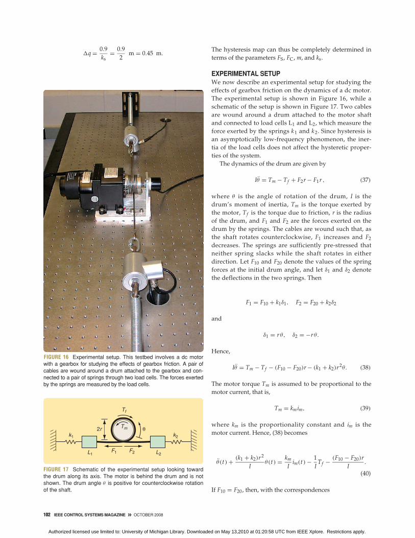
EXPERIMENTAL SETUPWe now describe an experimental setup for studying theeffects of gearbox friction on the dynamics of a dc motor.The experimental setup is shown in Figure 16, while aschematic of the setup is shown in Figure 17. Two cablesare wound around a drum attached to the motor shaftand connected to load cells L1 and L2, which measure theforce exerted by the springs k1 and k2. Since hysteresis isan asymptotically low-frequency phenomenon, the iner-tia of the load cells does not affect the hysteretic proper-ties of the system.

The dynamics of the drum are given by

Iθ = Tm − Tf + F2r − F1r , (37)

where θ is the angle of rotation of the drum, I is thedrum’s moment of inertia, Tm is the torque exerted bythe motor, Tf is the torque due to friction, r is the radiusof the drum, and F1 and F2 are the forces exerted on thedrum by the springs. The cables are wound such that, asthe shaft rotates counterclockwise, F1 increases and F2decreases. The springs are sufficiently pre-stressed thatneither spring slacks while the shaft rotates in eitherdirection. Let F10 and F20 denote the values of the springforces at the initial drum angle, and let δ1 and δ2 denotethe deflections in the two springs. Then

F1 = F10 + k1δ1, F2 = F20 + k2δ2

and

δ1 = rθ, δ2 = −rθ.

Hence,

Iθ = Tm − Tf − (F10 − F20)r − (k1 + k2)r2θ. (38)

The motor torque Tm is assumed to be proportional to themotor current, that is,

Tm = kmim, (39)

where km is the proportionality constant and im is themotor current. Hence, (38) becomes

θ (t) + (k1 + k2)r2

Iθ(t) = km

Iim(t) − 1

ITf − (F10 − F20)r

I.

(40)

If F10 = F20, then, with the correspondences

FIGURE 17 Schematic of the experimental setup looking towardthe drum along its axis. The motor is behind the drum and is notshown. The drum angle θ is positive for counterclockwise rotationof the shaft.

k2k1

L2F2F1L1

2r θTm

Tf

FIGURE 16 Experimental setup. This testbed involves a dc motorwith a gearbox for studying the effects of gearbox friction. A pair ofcables are wound around a drum attached to the gearbox and con-nected to a pair of springs through two load cells. The forces exertedby the springs are measured by the load cells.



ks

m= (k1 + k2)r2

I,

Fe

m= km

Iim,

Fm

= 1I

Tf , (41)

the dynamics in (40) are identical to the dynamics of themass-spring system (28).

The setup is connected to a digital computer through adSPACE 1103 system, which has one encoder, five analogto digital (A/D) channels, and five digital to analog (D/A)channels. Each load cell, whose output is amplified by anEndevco voltage amplifier model 136, can measure a maxi-mum load of 75 kg and has a sensitivity of 0.26 mV/kg. Theamplifier gain can be set between zero and 1000, and theamplified signals are sampled by the dSPACE system. Thedc motor has a built-in tachometer that measures the angu-lar velocity of the motor shaft. The angular velocity signalis read through an A/D channel. The conversion for thetachometer output is 0.01 V/rpm. A Heidenhain encodermeasures the angle of the drum. The gear ratio between themotor shaft and the drum is 1:68.8. Current is supplied tothe dc motor through a Quanser linear current amplifierLCAM. The required current profile is commanded to thecurrent amplifier through one of the D/A channels. The

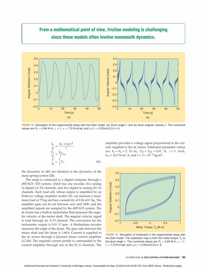
amplifier provides a voltage signal proportional to the cur-rent supplied to the dc motor. Estimated parameter valuesare k1 = k2 = 2 N/m, F10 = F20 = 0.01 N, r = 1 inch,km = 16.5 N-m/A, and I = 3 × 10−4 kg-m2.


FIGURE 18 Simulation of the experimental setup with the Dahl model. (a) Drum angle θ and (b) drum angular velocity θ . The numericalvalues are FC = 0.84 N-m, γ = 1, σ = 7.5 N-m/rad, and im(t ) = 0.05 sin(0.2π t) A.

0 10 20 30 40 50−0.2

−0.1

0

0.1

0.2

0.3

0.4

0.5

Time [s]

Ang

ular

Def

lect

ion

θ [r

ad]

(a)

0 10 20 30 40 50−0.4

−0.3

−0.2

−0.1

0

0.1

0.2

0.3

0.4

Time [s]

Ang

ular

Vel

ocity

[rad

/s]

(b)

FIGURE 19 Simulation of hysteresis in the experimental setup withthe Dahl model. The hysteresis map is from the motor torque Tm tothe drum angle θ . The numerical values are FC = 0.84 N-m, γ = 1,σ = 7.5 N-m/rad, and im(t ) = 0.05 sin(0.2π t) A.

−1 −0.5 0 0.5 1−0.2

−0.1

0

0.1

0.2

0.3

0.4

0.5

Ang

ular

Def

lect

ion

θ [r

ad]

Motor Torque Tm [N-m]

From a mathematical point of view, friction modeling is challenging

since these models often involve nonsmooth dynamics.


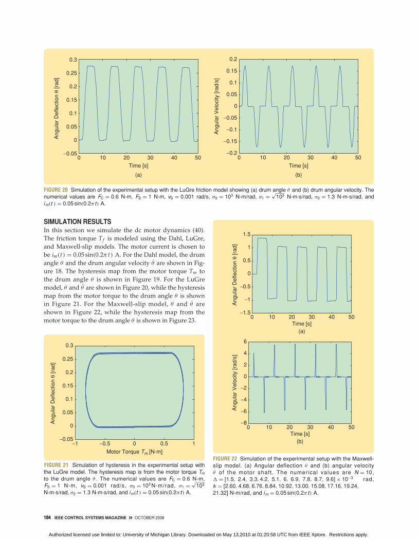
SIMULATION RESULTSIn this section we simulate the dc motor dynamics (40).The friction torque Tf is modeled using the Dahl, LuGre,and Maxwell-slip models. The motor current is chosen tobe im(t) = 0.05 sin(0.2π t) A. For the Dahl model, the drumangle θ and the drum angular velocity θ are shown in Fig-ure 18. The hysteresis map from the motor torque Tm tothe drum angle θ is shown in Figure 19. For the LuGremodel, θ and θ are shown in Figure 20, while the hysteresismap from the motor torque to the drum angle θ is shownin Figure 21. For the Maxwell-slip model, θ and θ areshown in Figure 22, while the hysteresis map from themotor torque to the drum angle θ is shown in Figure 23.

FIGURE 22 Simulation of the experimental setup with the Maxwell-slip model. (a) Angular deflection θ and (b) angular velocity θ of the motor shaft. The numerical values are N = 10,� = [1.5, 2.4, 3.3, 4.2, 5.1, 6, 6.9, 7.8, 8.7, 9.6] × 10−3 rad,k = [2.60, 4.68, 6.76, 8.84, 10.92, 13.00, 15.08, 17.16, 19.24,

21.32] N-m/rad, and im = 0.05 sin(0.2π t) A.

0 10 20 30 40 50−1.5

−1

−0.5

0

0.5

1

1.5

Time [s]

Ang

ular

Def

lect

ion

θ [r

ad]

(a)

0 10 20 30 40 50−8

−6

−4

−2

0

2

4

6

Time [s]

Ang

ular

Vel

ocity

[rad

/s]

(b)

FIGURE 21 Simulation of hysteresis in the experimental setup withthe LuGre model. The hysteresis map is from the motor torque Tm

to the drum angle θ . The numerical values are FC = 0.6 N-m,FS = 1 N-m, vS = 0.001 rad/s, σ0 = 103 N-m/rad, σ1 =

√103

N-m-s/rad, σ2 = 1.3 N-m-s/rad, and im(t ) = 0.05 sin(0.2π t) A.

−1 −0.5 0 0.5 1−0.05

0

0.05

0.1

0.15

0.2

0.25

0.3

Ang

ular

Def

lect

ion

θ [r

ad]


FIGURE 20 Simulation of the experimental setup with the LuGre friction model showing (a) drum angle θ and (b) drum angular velocity. Thenumerical values are FC = 0.6 N-m, FS = 1 N-m, vS = 0.001 rad/s, σ0 = 103 N-m/rad, σ1 =

√103 N-m-s/rad, σ2 = 1.3 N-m-s/rad, and

im(t ) = 0.05 sin(0.2π t) A.

0 10 20 30 40 50−0.05

0

0.05

0.1

0.15

0.2

0.25

0.3

Time [s]

Ang

ular

Def

lect

ion

θ [r

ad]

(a)

−0.2

−0.15

−0.1

−0.05

0

0.05

0.1

0.15

0.2

Time [s]

Ang

ular

Vel

ocity

[rad

/s]

0 10 20 30 40 50

(b)



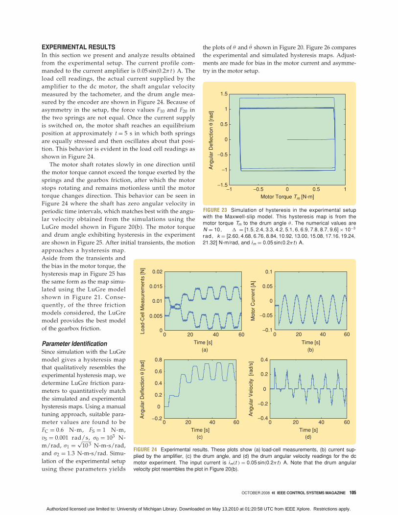
EXPERIMENTAL RESULTSIn this section we present and analyze results obtainedfrom the experimental setup. The current profile com-manded to the current amplifier is 0.05 sin(0.2π t) A. Theload cell readings, the actual current supplied by theamplifier to the dc motor, the shaft angular velocitymeasured by the tachometer, and the drum angle mea-sured by the encoder are shown in Figure 24. Because ofasymmetry in the setup, the force values F10 and F20 inthe two springs are not equal. Once the current supplyis switched on, the motor shaft reaches an equilibriumposition at approximately t = 5 s in which both springsare equally stressed and then oscillates about that posi-tion. This behavior is evident in the load cell readings asshown in Figure 24.

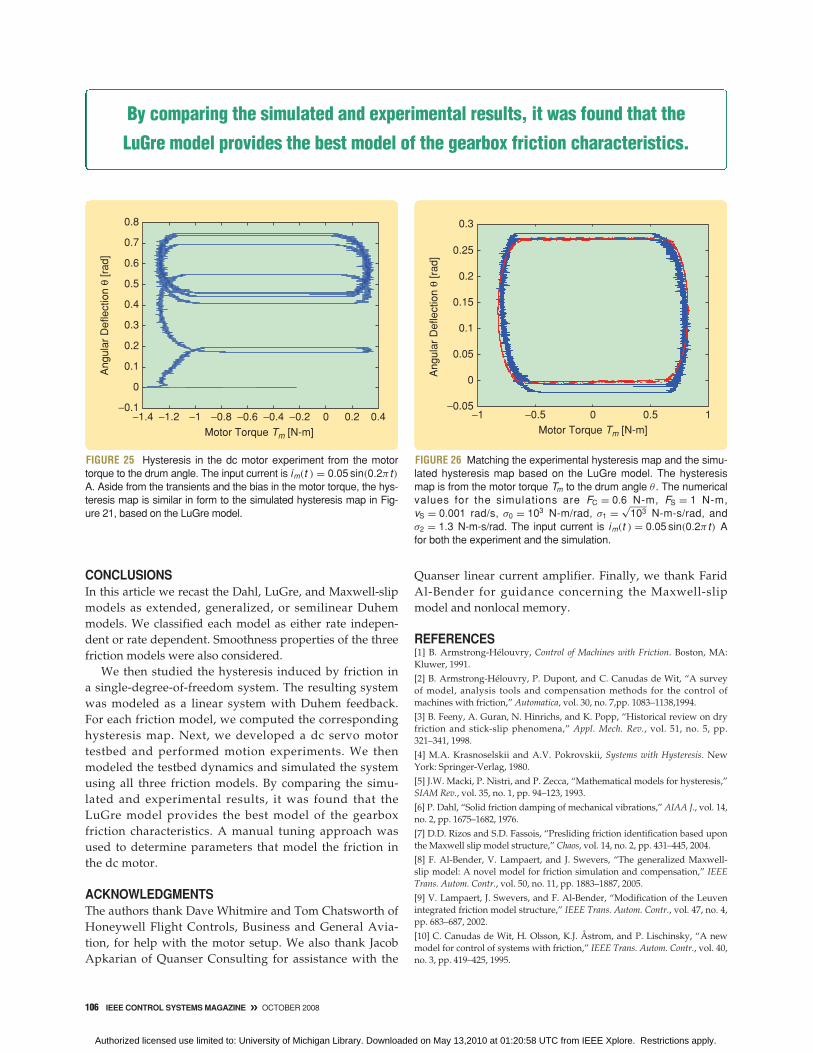
The motor shaft rotates slowly in one direction untilthe motor torque cannot exceed the torque exerted by thesprings and the gearbox friction, after which the motorstops rotating and remains motionless until the motortorque changes direction. This behavior can be seen inFigure 24 where the shaft has zero angular velocity inperiodic time intervals, which matches best with the angu-lar velocity obtained from the simulations using theLuGre model shown in Figure 20(b). The motor torqueand drum angle exhibiting hysteresis in the experimentare shown in Figure 25. After initial transients, the motionapproaches a hysteresis map.Aside from the transients andthe bias in the motor torque, thehysteresis map in Figure 25 hasthe same form as the map simu-lated using the LuGre modelshown in Figure 21. Conse-quently, of the three frictionmodels considered, the LuGremodel provides the best modelof the gearbox friction.

Parameter IdentificationSince simulation with the LuGremodel gives a hysteresis mapthat qualitatively resembles theexperimental hysteresis map, wedetermine LuGre friction para-meters to quantitatively matchthe simulated and experimentalhysteresis maps. Using a manualtuning approach, suitable para-meter values are found to beFC = 0.6 N-m, FS = 1 N-m,vS = 0.001 rad/s, σ0 = 103 N-m/rad, σ1 =

√10 3 N-m-s/rad,

and σ2 = 1.3 N-m-s/rad. Simu-lation of the experimental setupusing these parameters yields

the plots of θ and θ shown in Figure 20. Figure 26 comparesthe experimental and simulated hysteresis maps. Adjust-ments are made for bias in the motor current and asymme-try in the motor setup.

FIGURE 23 Simulation of hysteresis in the experimental setupwith the Maxwell-slip model. This hysteresis map is from themotor torque Tm to the drum angle θ . The numerical values areN = 10, � = [1.5, 2.4, 3.3, 4.2, 5.1, 6, 6.9, 7.8, 8.7, 9.6] × 10−3

rad, k = [2.60, 4.68, 6.76, 8.84, 10.92, 13.00, 15.08, 17.16, 19.24,

21.32] N-m/rad, and im = 0.05 sin(0.2π t) A.

−1 −0.5 0 0.5 1−1.5

−1

−0.5

0

0.5

1

1.5

Ang

ular

Def

lect

ion

θ [r

ad]


FIGURE 24 Experimental results. These plots show (a) load-cell measurements, (b) current sup-plied by the amplifier, (c) the drum angle, and (d) the drum angular velocity readings for the dcmotor experiment. The input current is im(t ) = 0.05 sin(0.2π t) A. Note that the drum angularvelocity plot resembles the plot in Figure 20(b).

0 20 40 600

0.005

0.01

0.015

0.02

Time [s]

Load

-Cel

l Mea

sure

men

ts [N

]

0 20 40 60−0.1

−0.05

0

0.05

0.1

Time [s]

Mot

or C

urre

nt [A

]

0 20 40 60−0.4

−0.2

0

0.2

0.4

Time [s]

Ang

ular

Vel

ocity

[ra

d/s]

0 20 40 60−0.2

0

0.2

0.4

0.6

0.8

Time [s]

Ang

ular

Def

lect

ion

θ [r

ad]

(a) (b)

(c) (d)



CONCLUSIONSIn this article we recast the Dahl, LuGre, and Maxwell-slipmodels as extended, generalized, or semilinear Duhemmodels. We classified each model as either rate indepen-dent or rate dependent. Smoothness properties of the threefriction models were also considered.

We then studied the hysteresis induced by friction ina single-degree-of-freedom system. The resulting systemwas modeled as a linear system with Duhem feedback.For each friction model, we computed the correspondinghysteresis map. Next, we developed a dc servo motortestbed and performed motion experiments. We thenmodeled the testbed dynamics and simulated the systemusing all three friction models. By comparing the simu-lated and experimental results, it was found that theLuGre model provides the best model of the gearboxfriction characteristics. A manual tuning approach wasused to determine parameters that model the friction inthe dc motor.

ACKNOWLEDGMENTSThe authors thank Dave Whitmire and Tom Chatsworth ofHoneywell Flight Controls, Business and General Avia-tion, for help with the motor setup. We also thank JacobApkarian of Quanser Consulting for assistance with the

Quanser linear current amplifier. Finally, we thank FaridAl-Bender for guidance concerning the Maxwell-slipmodel and nonlocal memory.

REFERENCES[1] B. Armstrong-Hélouvry, Control of Machines with Friction. Boston, MA:Kluwer, 1991.

[2] B. Armstrong-Hélouvry, P. Dupont, and C. Canudas de Wit, “A surveyof model, analysis tools and compensation methods for the control ofmachines with friction,” Automatica, vol. 30, no. 7,pp. 1083–1138,1994.

[3] B. Feeny, A. Guran, N. Hinrichs, and K. Popp, “Historical review on dryfriction and stick-slip phenomena,” Appl. Mech. Rev., vol. 51, no. 5, pp.321–341, 1998.

[4] M.A. Krasnoselskii and A.V. Pokrovskii, Systems with Hysteresis. NewYork: Springer-Verlag, 1980.

[5] J.W. Macki, P. Nistri, and P. Zecca, “Mathematical models for hysteresis,”SIAM Rev., vol. 35, no. 1, pp. 94–123, 1993.

[6] P. Dahl, “Solid friction damping of mechanical vibrations,” AIAA J., vol. 14,no. 2, pp. 1675–1682, 1976.

[7] D.D. Rizos and S.D. Fassois, “Presliding friction identification based uponthe Maxwell slip model structure,” Chaos, vol. 14, no. 2, pp. 431–445, 2004.

[8] F. Al-Bender, V. Lampaert, and J. Swevers, “The generalized Maxwell-slip model: A novel model for friction simulation and compensation,” IEEETrans. Autom. Contr., vol. 50, no. 11, pp. 1883–1887, 2005.

[9] V. Lampaert, J. Swevers, and F. Al-Bender, “Modification of the Leuvenintegrated friction model structure,” IEEE Trans. Autom. Contr., vol. 47, no. 4,pp. 683–687, 2002.

[10] C. Canudas de Wit, H. Olsson, K.J. Åstrom, and P. Lischinsky, “A newmodel for control of systems with friction,” IEEE Trans. Autom. Contr., vol. 40,no. 3, pp. 419–425, 1995.

FIGURE 25 Hysteresis in the dc motor experiment from the motortorque to the drum angle. The input current is im(t ) = 0.05 sin(0.2π t)A. Aside from the transients and the bias in the motor torque, the hys-teresis map is similar in form to the simulated hysteresis map in Fig-ure 21, based on the LuGre model.

−1.4 −1.2 −1 −0.8 −0.6 −0.4 −0.2 0 0.2 0.4−0.1

0

0.1

0.2

0.3

0.4

0.5

0.6

0.7

0.8

Ang

ular

Def

lect

ion

θ [r

ad]


FIGURE 26 Matching the experimental hysteresis map and the simu-lated hysteresis map based on the LuGre model. The hysteresismap is from the motor torque Tm to the drum angle θ . The numericalvalues for the simulations are FC = 0.6 N-m, FS = 1 N-m,vS = 0.001 rad/s, σ0 = 103 N-m/rad, σ1 =

√103 N-m-s/rad, and

σ2 = 1.3 N-m-s/rad. The input current is im(t ) = 0.05 sin(0.2π t) Afor both the experiment and the simulation.

−1 −0.5 0 0.5 1−0.05

0

0.05

0.1

0.15

0.2

0.25

0.3

Ang

ular

Def

lect

ion

θ [r

ad]


By comparing the simulated and experimental results, it was found that the

LuGre model provides the best model of the gearbox friction characteristics.



[11] J. Swevers, F. Al-Bender, C.G. Ganseman, and T. Prajogo, “An integratedfriction model structure with improved presliding behavior for accurate fric-tion compensation,” IEEE Trans. Autom. Contr., vol. 45, no. 4, pp. 675–686, 2000.[12] F. Al-Bender, V. Lampaert, and J. Swevers, “Modeling of dry slidingfriction dynamics: From heuristic models to physically motivated modelsand back,” Chaos, vol. 14, no. 2, pp. 446–445, 2004.[13] F. Al-Bender, V. Lampaert, S.D. Fassois, D.D. Rizos, K. Worden, D. Engster,A. Hornstein, and U. Parlitz, “Measurement and identification of pre-slidingfriction dynamics,” in Nonlinear Dynamics of Production Systems, G. Radons andR. Neugebauer, Eds. Weinheim: Wiley, 2004, pp. 349–367. [14] G. Ferretti, G. Magnani, and P. Rocco, “Single and multistate integralfriction models,” IEEE Trans. Autom. Contr., vol. 49, no. 12, pp. 2292–2297,2004.[15] J. Amin, B. Friedland, and A. Harnoy, “Implementation of a friction esti-mation and compensation technique,” IEEE Contr. Sys. Mag., vol. 17, no. 4,pp. 71–76, 1997.[16] S.C. Southward, C.J. Radcliffe, and C.R. MacCluer, “Robust nonlinearstick-slip friction compensation,” J. Dynam. Syst. Meas. Contr., vol. 113, no. 4,pp. 639–645, 1991.[17] S.-W. Lee and J.-H. Kim, “Robust adaptive stick-slip friction compensa-tion,” IEEE Trans. Ind. Electron., vol. 42, no. 5, pp. 474–479, 1995.[18] R.-H. Wu and P.-C. Tung, “Studies of stick-slip friction, preslidingdisplacement, and hunting,” J. Dynam. Syst., Meas. Contr., vol. 124, no. 1,pp. 111–117, 2002.[19] M. Marques, Differential Inclusions in Nonsmooth Mechanical Problems:Shocks and Dry Friction. Cambridge, MA: Birkhaüser, 1993.[20] S.P. Bhat and D.S. Bernstein, “Finite-time stability of continuousautonomous systems,” SIAM J. Contr. Optimiz., vol. 38, pp. 751–766, 2000.[21] S.P. Bhat and D.S. Bernstein, “Continuous finite-time stabilization of thetranslational and rotational double integrators,” IEEE Trans. Autom. Contr.,vol. 43, no. 5, pp. 678–682, 1998.[22] J. Oh and D.S. Bernstein, “Step convergence analysis of nonlinearfeedback hysteresis models,” in Proc. American Control Conf., Portland, OR,2005, pp. 697–702.[23] D. Angeli and E.D. Sontag, “Multi-stability in monotone input/outputsystems,” Sys. Contr. Lett., vol. 51, pp. 185–202, 2004.[24] D. Angeli, J.E. Ferrell, and E.D. Sontag, “Detection of multistability,bifurcations, and hysteresis in a large class of biological positive feedbacksystems,” in Proc. Nat. Academy Science, 2004, vol. 101, no. 7, pp. 1822–1827.[25] J. Oh and D.S. Bernstein, “Semilinear Duhem model for rate-independentand rate-dependent hysteresis,” IEEE Trans. Autom. Contr., vol. 50, no. 5,pp. 631–645, 2005.[26] A. Visintin, Differential Models of Hysteresis. New York: Springer-Verlag, 1994.[27] P.A. Bliman, “Mathematical study of the Dahl’s friction model,” Euro. J.Mech. Solids, vol. 11, no. 6, pp. 835–848, 1992.[28] Y.Q. Ni, Z.G. Ying, J.M. Ko, and W.Q. Zhu, “Random response of inte-grable Duhem hysteretic systems under non-white excitation,” Int. J. Non-Linear Mech., vol. 37, no. 8, pp. 1407–1419, 2002.[29] N. Barabanov and R. Ortega, “Necessary and sufficient conditions forpassivity of the LuGre friction model,” IEEE Trans. Autom. Contr., vol. 45,no. 4, pp. 830–832, 2000.[30] J. Swevers, F. Al-Bender, C. Ganseman, and T. Projogo, “An integratedfriction model structure with improved presliding behavior for accurate fric-tion compensation,” IEEE Trans. Autom. Contr., vol. 45, no. 4, pp. 675–686,2000.[31] F. Altpeter, “Friction modeling, identification and compensation,” Ph.D.dissertation, Ecole Polytechnique Federale de Lausanne, 1999 [Online]. Avail-able:http://biblion.epfl.ch/EPFL/theses/1999/1988/EPFL_TH1988.pdf. [32] S.L. Lacy, D.S. Bernstein, and S.P. Bhat, “Hysteretic systems and step-convergent semistability,” in Proc. American Control Conf., Chicago, IL, June2000, pp. 4139–4143.

AUTHOR INFORMATIONAshwani K. Padthe received the bachelor’s degree in aero-space engineering from the Indian Institute of TechnologyBombay in 2003. In 2006 he received the M.S. in aerospaceengineering at the University of Michigan, where he is

now pursuing the Ph.D. His research interests include hys-teretic systems and aeroelasticity.

Bojana Drincic received the bachelor’s degree inaerospace engineering from the University of Texas atAustin in 2007. She is now pursuing a Ph.D. at the Uni-versity of Michigan. Her research interests include hys-teretic systems, systems with friction, and spacecraftdynamics and control.

JinHyoung Oh received the bachelor’s degree in controland instrumentation engineering from Korea Universityand master’s degrees in aerospace engineering and appliedmathematics from Georgia Institute of Technology. Hereceived the Ph.D. in aerospace engineering from the Uni-versity of Michigan in 2005. He is currently employed byAutoLiv as a research engineer.

Demosthenis D. Rizos received the diploma in mechan-ical engineering from the University of Patras in 1999,where he is a doctoral candidate. His research interests arein experimental modal analysis, identification of linear andnonlinear mechanical systems, systems with friction, andfault detection and identification. He has contributed toseveral sponsored research projects and is a coauthor ofmore than 15 publications.

Spilios D. Fassois received the diploma in mechani-cal engineering from the National Technical Universityof Athens, Greece, in 1982, and the Ph.D. in mechanicalengineering from the University of Wisconsin-Madisonin 1986. He served on the faculty of the Department ofMechanical Engineering and Applied Mechanics of theUniversity of Michigan from 1986 to 1994 and is current-ly on the faculty of the Department of Mechanical andAeronautical Engineering of the University of Patras,Greece. His research interests are in the area of stochas-tic mechanical systems, including vibrating systems,with an emphasis on identification and fault detection.He leads the Stochastic Mechanical Systems andAutomation (SMSA) Laboratory at the University ofPatras and is the author of more than 130 publications.His research has been supported by Ford, EastmanKodak, General Motors, Whirlpool, Hellenic Aerospace,Hellenic Railways, Alenia, BAE Systems, and Volkswa-genstiftung. He is a member of the editorial board of theJournal of Mechanical Systems and Signal Processing, andhe was a guest editor for the special section on systemidentification in the October 2007 issue of IEEE ControlSystems Magazine.

Dennis S. Bernstein ([email protected]) is a professorin the Aerospace Engineering Department at the Universi-ty of Michigan. He is editor-in-chief of IEEE Control Sys-tems Magazine and the author of Matrix Mathematics(Princeton University Press). His interests are in systemidentification and adaptive control for aerospace applica-tions. He can be contacted at the University of Michigan,Aerospace Engineering Department, 1320 Beal Ave., AnnArbor, MI 48109-2140 USA.



Documents

EXPERIMENTAL DETERMINATION OF GEARBOX …dsbaero/library/DuhemModelingofHysteresi… · importance, and the associated literature is vast; ... The testbed consists of a dc motor with