1

Experimental Design StrategiesRob MacCoun

CSLS Miniseries in Empirical Research Methods, 5 Nov 2010

Roadmap• If experiments are the answer, what is the

question?• Counterfactuals • Internal validity• External validity; mundane vs. exp realism• Construct validity• Statistical conclusion validity

There are various technical appendix slides at the end of the handout.

2

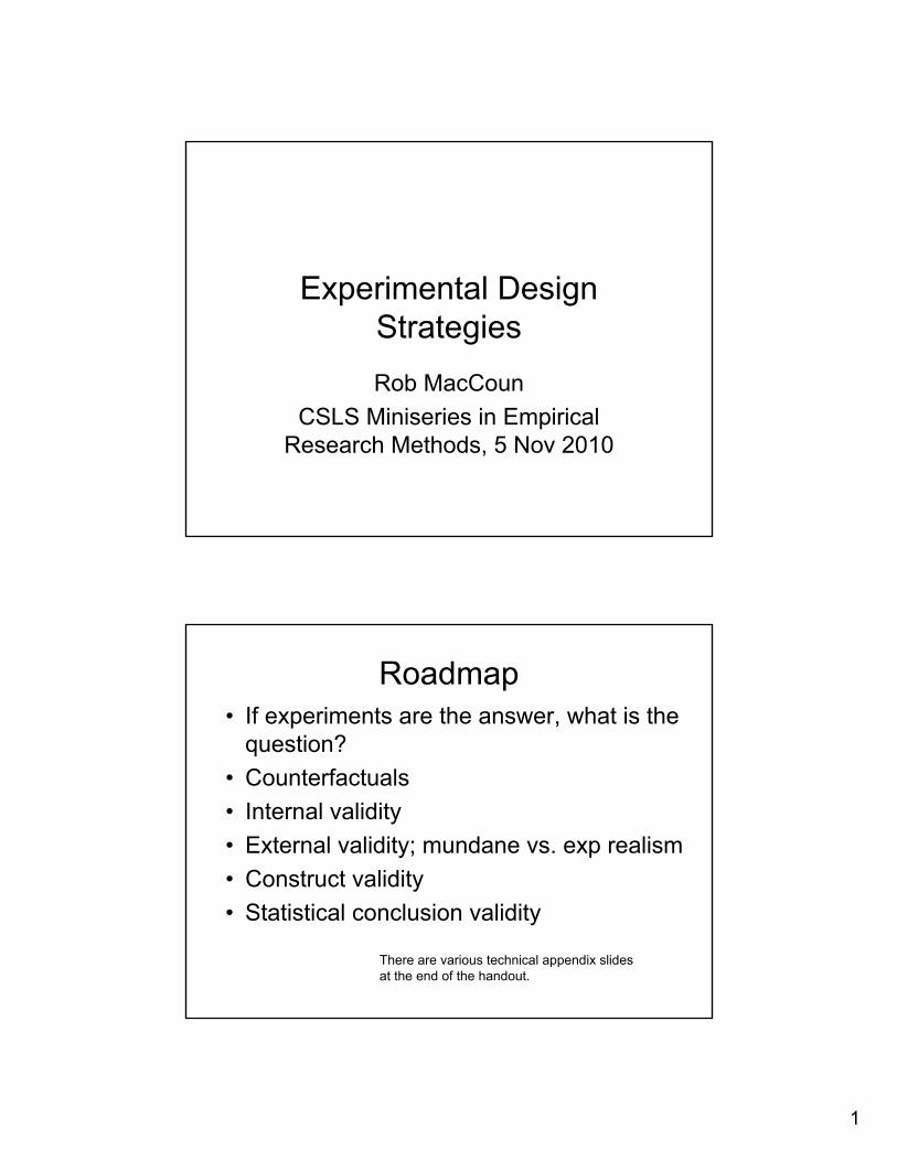
What experiments offer• Great for:

– Causal inference (why are A and B correlated?)– Theory testing– Low-risk test of interventions that haven’t been

adopted in the real world (e.g., change of law or new procedure)

• Bad when:– Goal is point estimation (forecasting, etc.)– External validity is more important than internal

validity– Ethical, political, legal barriers

Juries appear to treat corporations differently

(Chin & Peterson, 1985 archival analysis)

0%

10%

20%

30%

40%

50%

60%

Liability$0

$30,000

$60,000

$90,000

$120,000

$150,000

$180,000

Awards

Individuals

Corporations

Individuals

Corporations

3

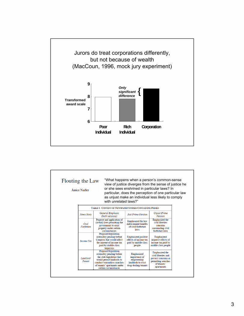
6

7

8

9

Poor Individual

Rich Individual

Corporation

Transformedaward scale

Onlysignificantdifference

Jurors do treat corporations differently, but not because of wealth

(MacCoun, 1996, mock jury experiment)

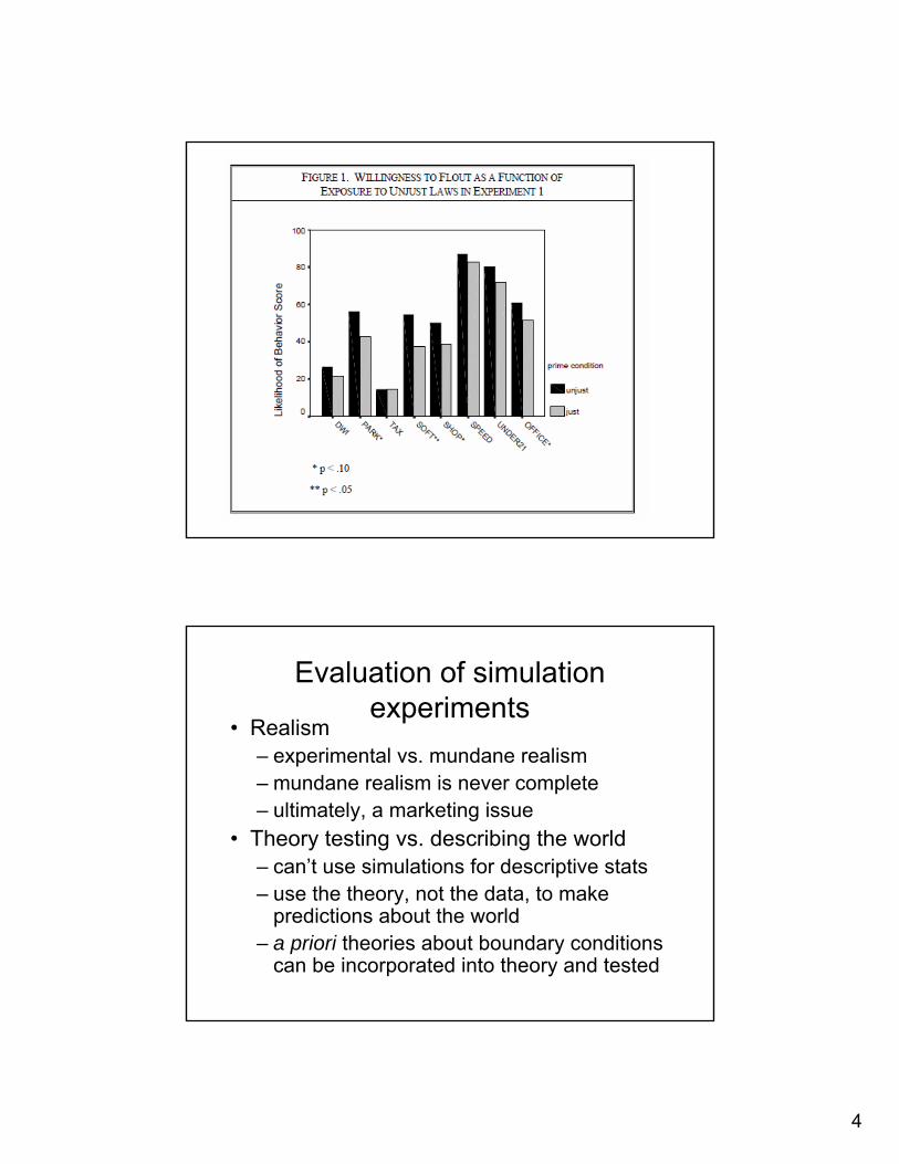
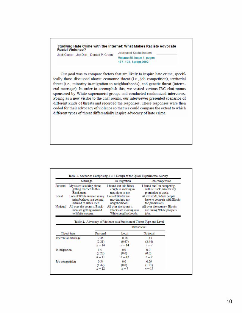
“What happens when a person’s common-sense view of justice diverges from the sense of justice he or she sees enshrined in particular laws? In particular, does the perception of one particular law as unjust make an individual less likely to comply with unrelated laws?”

4

Evaluation of simulation experiments

• Realism– experimental vs. mundane realism– mundane realism is never complete– ultimately, a marketing issue

• Theory testing vs. describing the world– can’t use simulations for descriptive stats– use the theory, not the data, to make

predictions about the world– a priori theories about boundary conditions

can be incorporated into theory and tested

5

Cohen, Nisbett, Bowdle, & Schwarz (1996): “Participants were University of Michigan students who grew up in the North or South. In 3 experiments, they were insulted by a confederate who bumped into the participant and called him an “asshole.”

Two diverging theories

• The ‘confidence heuristic’– Highly confident advisors are presumed to be more

accurate, knowledgeable, and credible, even when given feedback that demonstrates otherwise (Price & Stone, 2004).

• The ‘calibration hypothesis’– Advisors are perceived more credible if they express

confidence only when warranted - highly confident but inaccurate advisors lose credibility (Tenney, MacCoun, Spellman, & Hastie, 2007).

6

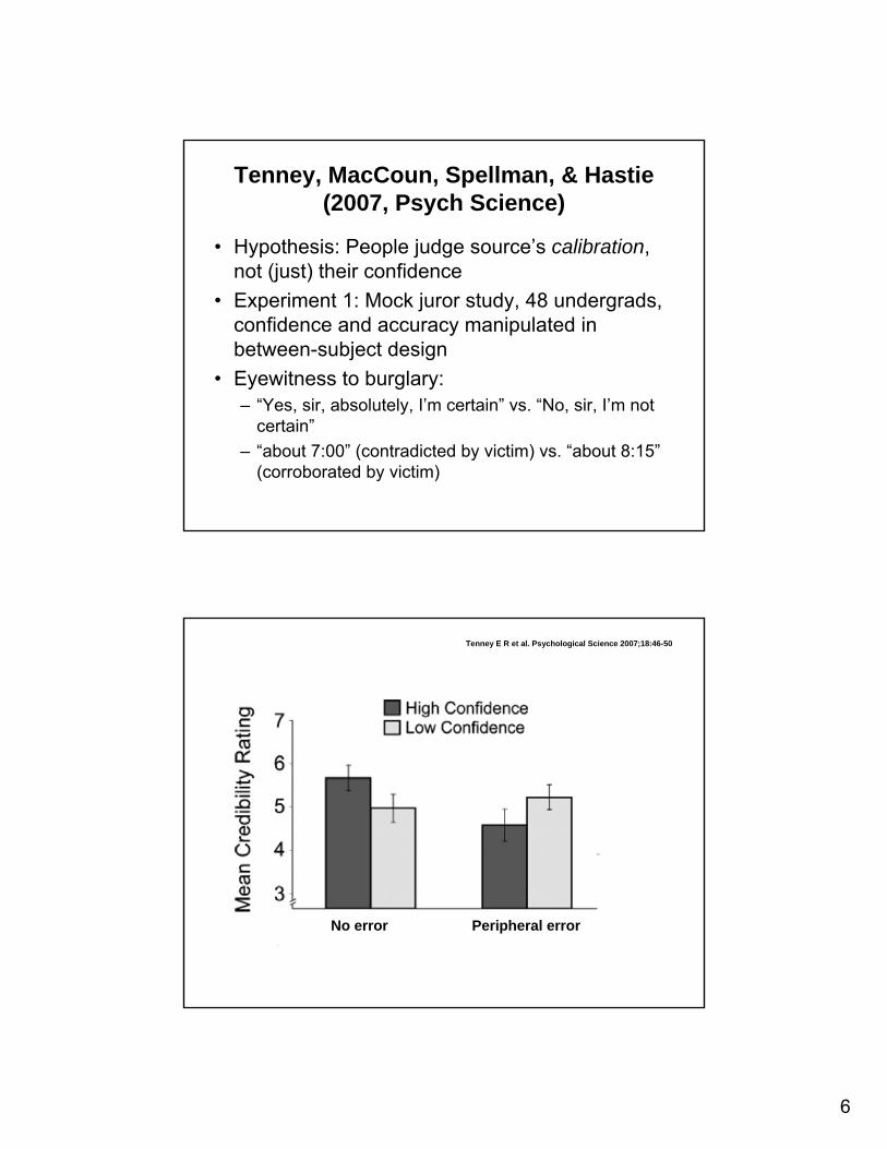
Tenney, MacCoun, Spellman, & Hastie(2007, Psych Science)

• Hypothesis: People judge source’s calibration, not (just) their confidence

• Experiment 1: Mock juror study, 48 undergrads, confidence and accuracy manipulated in between-subject design

• Eyewitness to burglary:– “Yes, sir, absolutely, I’m certain” vs. “No, sir, I’m not

certain”– “about 7:00” (contradicted by victim) vs. “about 8:15”

(corroborated by victim)

Tenney E R et al. Psychological Science 2007;18:46-50

No error Peripheral error

7

Tenney, Spellman, & MacCoun (2008, JESP): Exp. 1

• Cautiousness, not calibration? – Maybe in the presence of errors people prefer

informants who are more modest, or cautious, in their claims overall.

• Well-calibrated: Cautious witness is correct about high-confidence assertion and wrong about the low-confidence assertion (as in Tenney et al., 2007)

• Poorly-calibrated: Cautious witness is correct about the low-confidence assertion and wrong about the high-confidence assertion

8

Exp. 2• What if there is a good reason for a high-confidence

error?– Justifiable error should not affect perceived credibility

• Time 1: Two witnesses identify suspect as passenger in vehicle -- one with confidence, the other cautiously– CONFIDENT > CAUTIOUS

• Time 2: Both shown to be in error (Time 2) about the identification– BOTH WITNESSES LOSE CREDIBILITY

• Time 3: A justification for the error is given: the passenger had an identical twin!– CAUTIOUS WITNESS REGAINS CREDIBILITY

Ethical and political problems with randomization

• Withholding possible benefit from controls?– cancelling study midstream raises threats to statistical

conclusion validity (discussed later)

• Exposing treatment group to extra hardships, risks?– informed consent creates selection bias, expectancy

effects• “Equipoise” criterion in medical research• Lotteries as a fair allocation rule when there is

scarcity

9

Some patients were randomly assigned to a placebo surgery condition in which “three 1-cm incisions were made in the skin.” “…Incisional erythema developed in one patient, who was given antibiotics. In a second patient, calf swelling developed in the leg that had undergone surgery; venography was negative for thrombosis.”

10

11

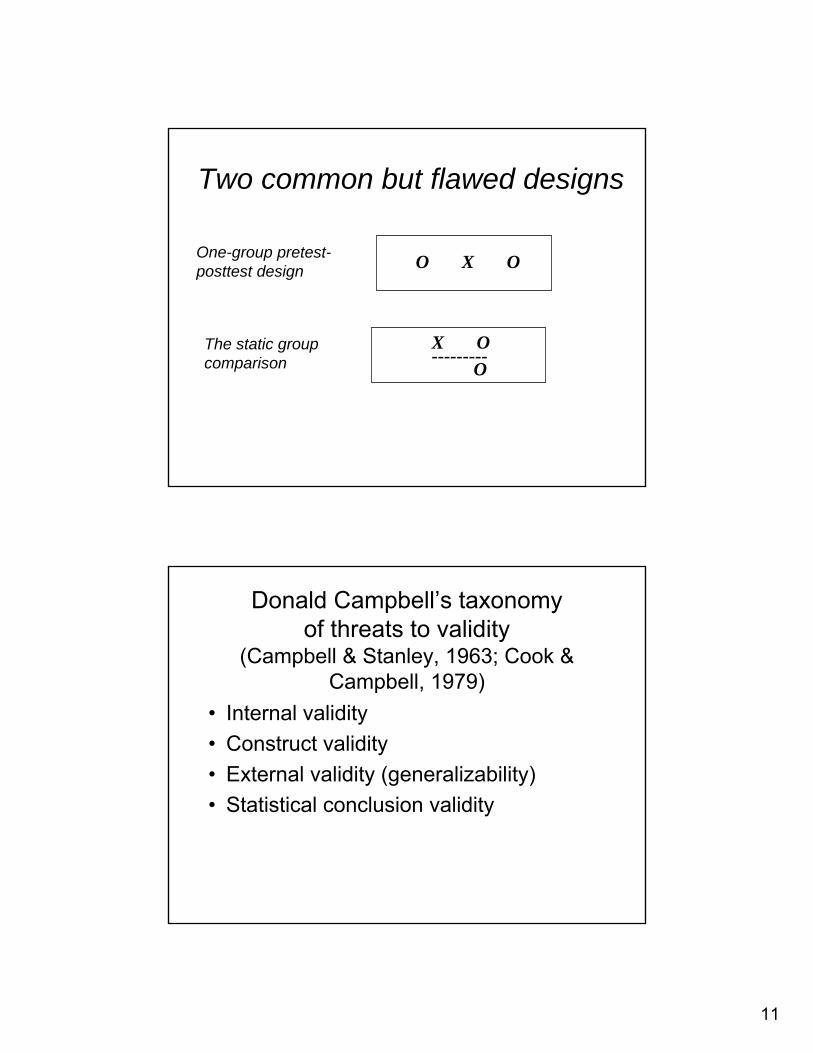
Two common but flawed designs

O X O

X O---------

O

One-group pretest-posttest design

The static group comparison

Donald Campbell’s taxonomy of threats to validity

(Campbell & Stanley, 1963; Cook & Campbell, 1979)

• Internal validity• Construct validity• External validity (generalizability)• Statistical conclusion validity

12

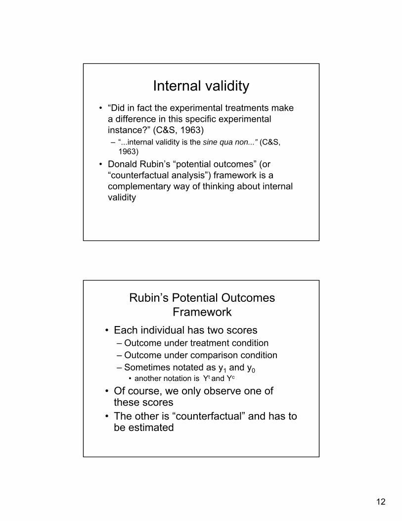
Internal validity• “Did in fact the experimental treatments make

a difference in this specific experimental instance?” (C&S, 1963)– “...internal validity is the sine qua non...” (C&S,

1963)• Donald Rubin’s “potential outcomes” (or

“counterfactual analysis”) framework is a complementary way of thinking about internal validity

Rubin’s Potential Outcomes Framework

• Each individual has two scores– Outcome under treatment condition – Outcome under comparison condition – Sometimes notated as y1 and y0

• another notation is Yt and Yc

• Of course, we only observe one of these scores

• The other is “counterfactual” and has to be estimated

13

Threats to internal validity1. History2. Maturation3. Testing4. Instrumentation5. Statistical regression (to the mean)6. Selection7. Mortality (differential attrition)

1) History• Specific events occuring between the

first and second measurement in addition to the treatment variable

• Examples:– highly publicized events– exposure to other (non-study) treatments

14

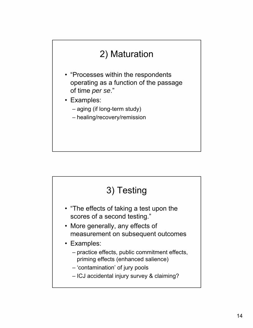
2) Maturation

• “Processes within the respondents operating as a function of the passage of time per se.”

• Examples:– aging (if long-term study)– healing/recovery/remission

3) Testing

• “The effects of taking a test upon the scores of a second testing.”

• More generally, any effects of measurement on subsequent outcomes

• Examples:– practice effects, public commitment effects,

priming effects (enhanced salience)– ‘contamination’ of jury pools– ICJ accidental injury survey & claiming?

15

4) Instrumentation

• Changes in the measuring instrument (or the observer) that produce changes in the obtained measurements

• Examples:– personnel changes in interview staff– changes in coders’ standards over time– mid-stream revisions in survey questions

or procedures– addition of video or audio recording

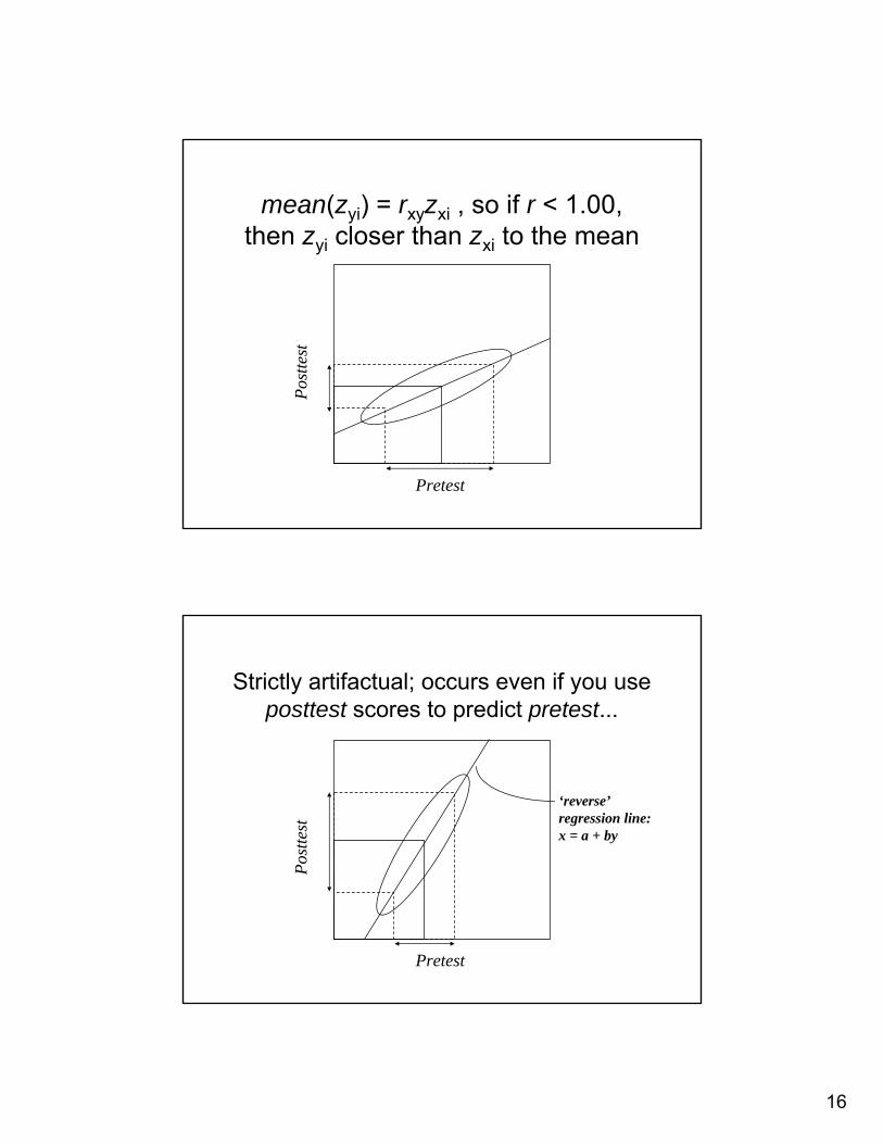
5) Regression to the mean

• Occurs when groups are selected based on extreme (high &/or low) pretest scores

• If less than perfect pretest-posttest correlation, posttest scores will be closer to mean, regardless of treatment

• Thus ‘the best’ will get worse, ‘the worst’ will get better

16

mean(zyi) = rxyzxi , so if r < 1.00, then zyi closer than zxi to the mean

Pretest

Post

test

Strictly artifactual; occurs even if you use posttest scores to predict pretest...

Pretest

Post

test

‘reverse’regression line:x = a + by

17

6) Selection• Occurs when different processes of

recruitment to comparison groups– can be artifact of research protocol– can be due to respondent self-selection

• Examples:– students in Catholic vs. public schools– addicts in treatment vs. not in treatment– effects of pregancy on employment, etc.

• Econometric solutions (Heckman)

7) ‘Mortality’ (differential attrition)

• Differential attrition from study conditions prior to posttest data

• Involves same concerns raised by nonresponse in surveys

• In essence, “selection out” rather than “selection in”

18

Strategy 1: Simple matching• Create a comparison group by selecting

other cases matched on demographics, etc.– Often misnamed a “control group”

• Better than no comparison, but still flawed– can never establish that you’ve matched

on every relevant variable– Modern matching via “propensity scores” is

stronger, but no panacea

Strategy 2: Random assignment• R. A. Fisher (1926): agricultural

experiments• Doesn’t require any explicit matching• Law of large numbers implies that given

sufficiently large samples, no reason to expect any pretreatment differences except by chance

• (By chance, may have pretest diff’s)

19

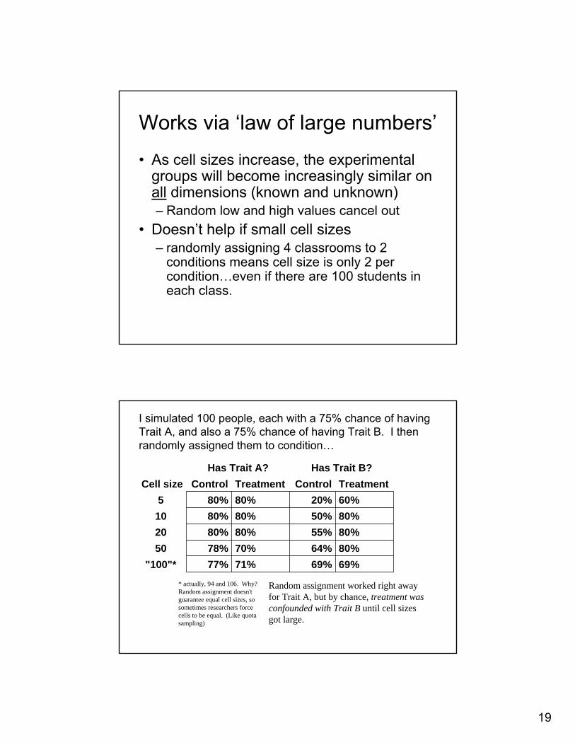
Works via ‘law of large numbers’

• As cell sizes increase, the experimental groups will become increasingly similar on all dimensions (known and unknown)– Random low and high values cancel out

• Doesn’t help if small cell sizes– randomly assigning 4 classrooms to 2

conditions means cell size is only 2 per condition…even if there are 100 students in each class.

I simulated 100 people, each with a 75% chance of having Trait A, and also a 75% chance of having Trait B. I then randomly assigned them to condition…

Random assignment worked right away for Trait A, but by chance, treatment was confounded with Trait B until cell sizes got large.

69%69%71%77%"100"*80%64%70%78%5080%55%80%80%2080%50%80%80%1060%20%80%80%5TreatmentControlTreatmentControlCell size

Has Trait B?Has Trait A?

* actually, 94 and 106. Why? Random assignment doesn'tguarantee equal cell sizes, so sometimes researchers force cells to be equal. (Like quota sampling)

20

“Natural Experiments”

• Sometimes interventions get allocated via random or quasi-random processes– Exogenous shocks – effect of Afghan invasion on street price of

heroin• Rarely truly random, so need to carefully

test for treatment confounds– Vietnam draft lottery

Pretest-posttest control group design

• Very strong for internal validity, though pretesting raise testing concerns regarding external validity

R O X OR O O

21

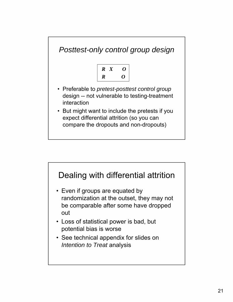
Posttest-only control group design

• Preferable to pretest-posttest control groupdesign -- not vulnerable to testing-treatment interaction

• But might want to include the pretests if you expect differential attrition (so you can compare the dropouts and non-dropouts)

R X OR O

Dealing with differential attrition

• Even if groups are equated by randomization at the outset, they may not be comparable after some have dropped out

• Loss of statistical power is bad, but potential bias is worse

• See technical appendix for slides on Intention to Treat analysis

22

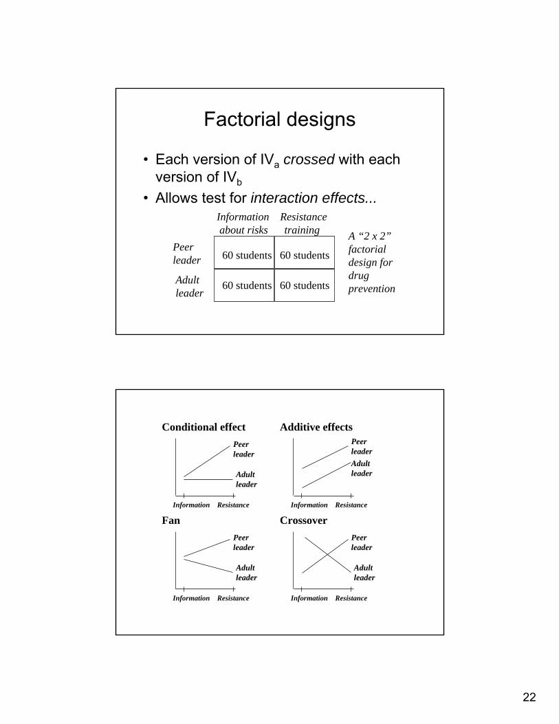
Factorial designs

• Each version of IVa crossed with each version of IVb

• Allows test for interaction effects...Information Resistanceabout risks training

Peerleader

Adultleader

60 students 60 students

60 students 60 students

A “2 x 2”factorialdesign fordrug prevention

Information Resistance

Peer leader

Adult leader

Conditional effect

Information Resistance

Peer leader

Adult leader

Fan

Information Resistance

Peer leader

Adult leader

CrossoverInformation Resistance

Peer leaderAdult leader

Additive effects

23

Additional design variants• Between-subjects vs. within-subjects (‘repeated

measures’) designs– Between: each person exposed to single condition

(single level of IV)– Within: each person exposed to multiple levels of

IV (essential to counterbalance order)• Nested designs

– e.g., randomly assign class to condition; students nested within class

• Intentionally confounded designs (for economy):– Latin-squares, hyper-graeco-latin squares,

fractional factorials, etc.

Parametric designs

• Simply comparing two levels of a variable will not tell you about its functional form– E.g, diminishing marginal utility, U-shaped

relationships, S-shaped dose-response curves

• E.g., Prospect theory vs. alternative theories

– If you choose two locations on the “wrong” part of the curve, you might reach misleading inferences

24

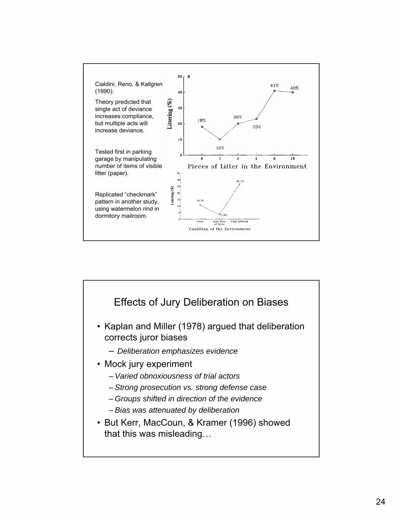
Cialdini, Reno, & Kallgren(1990):

Theory predicted that single act of deviance increases compliance, but multiple acts will increase deviance.

Tested first in parking garage by manipulating number of items of visible litter (paper).

Replicated “checkmark” pattern in another study, using watermelon rind in dormitory mailroom.

Effects of Jury Deliberation on Biases

• Kaplan and Miller (1978) argued that deliberation corrects juror biases– Deliberation emphasizes evidence

• Mock jury experiment– Varied obnoxiousness of trial actors– Strong prosecution vs. strong defense case– Groups shifted in direction of the evidence– Bias was attenuated by deliberation

• But Kerr, MacCoun, & Kramer (1996) showed that this was misleading…

25

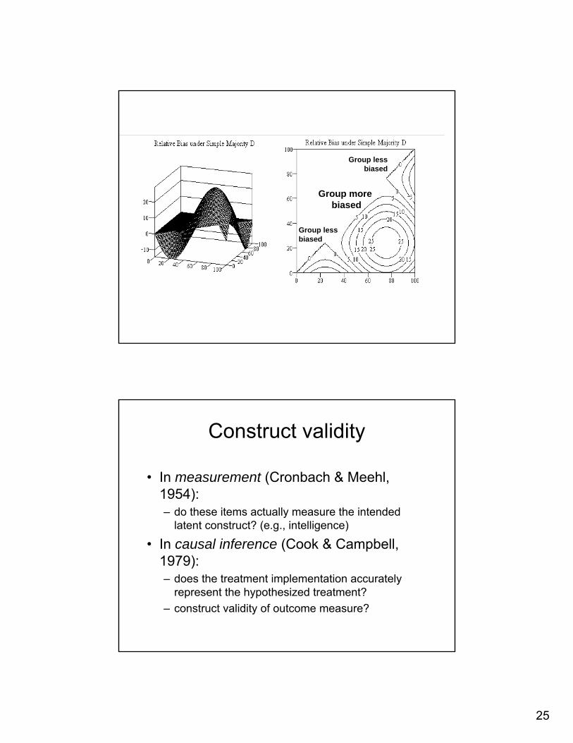
Group more biased

Group lessbiased

Group lessbiased

Construct validity

• In measurement (Cronbach & Meehl, 1954):– do these items actually measure the intended

latent construct? (e.g., intelligence)

• In causal inference (Cook & Campbell, 1979):– does the treatment implementation accurately

represent the hypothesized treatment?– construct validity of outcome measure?

26

Treatment confounds• Not explicitly listed in C&S, but extremely

common problem in experiments• In essence, if ‘treatment’ involved more than one

‘thing’, which was the cause?• Examples:

– different sites or different administrators– treatment involves multiple program elements– treatment group asked extra questions– ‘Hawthorne’ effect

• May require special control groups

Lab studies show that sequential lineups are fairer than simultaneous lineups.

But controversial Illinois State Police pilot program experiment claimed to find the opposite…

47%38%No ID9%3%Filler ID

45%60%Suspect ID

Sequential presentation (n=229)

Simultaneous presentation (n=319)

27

Gary Wells’ critique

• “My main reaction to this report is disappointment and concern that the design of the study does not permit any clear conclusions. The reason is…because the simultaneous lineups never used the double-blind procedure whereas the sequential lineups alwaysused the double-blind procedure.”

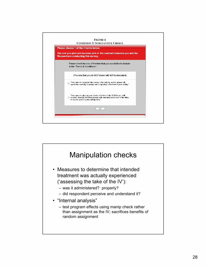
Web survey with 480 questions spread out over 480 separate pop-up web pages! How many will participants actually complete?

Conventional boilerplate version: 7-paragraph standard end-user contract with “consent to participate” check box.

Substantive choice version: Given two choices (NEXT SLIDE)…

“Results of an online experiment reveal that marginal participation in contract drafting increases drafters’ performance of an undesirable contract term.”

Problem: Confounded substantive choice with salience of requirements.

28

Manipulation checks

• Measures to determine that intended treatment was actually experienced (‘assessing the take of the IV’):– was it administered? properly?– did respondent perceive and understand it?

• “Internal analysis”– test program effects using manip check rather

than assignment as the IV; sacrifices benefits of random assignment

29

Mediation model

X1 X2 X3

Jobskills

e1 e2 e3

X4 X5 X6

Socio-economic

status

e4 e5 e6

Jobtraining

Treatment Mediating process Outcome

Any directeffect on SES shoulddisappearafter controllingfor job skills

Ideally, use multiple indicators (Xs) for each construct

Expectancy effects• Hypothesis guessing, ‘demand

characteristics’– respondent modifies responses to try to help or

hinder researcher– Orne (1962): S’s worked for 5 hours summing

random #s– can require ‘cover stories’, single blind designs,

placebos

• Experimenter expectancy effects– Rosenthal: gave E’s hypotheses, biased results

even when E only read instructions– requires double blind designs

30

Problem of failing to reject the null

• Karl Popper: Can only falsify a theory; can’t ‘confirm’ it

• Fisher: Can only reject the null, can’t confirm it– problem: the null is rarely your hypothesis– can we ever know for sure there’s “no effect”?

• Failure to reject null could be due to:– small sample size– weak instantiation of an effective treatment– noisy measurement

Risk of using non-experimental approaches? Glazerman, Levy, & Myers (2003)

• 12 case studies on social welfare with:– An experimental evaluation– 1+ non-experimental (NX) evaluations

• Size of bias (in 1996$ of annual earnings):– Regression: $1,101 (about 10% of annual

earnings)– Matching: $1,143– Selection or instrumental variables: $2,791

• “potential for very large bias”

31

Wilde & Hollister (2007)

• Project STAR – Tennessee class size experiment– Experimental data from 12 schools– Compared to use of propensity score methods for

each site• Estimates were >10 percentile points apart for 8

of 12 schools• Based on cost-effectiveness criteria, “the

nonexperimental estimate would have led to the wrong conclusion in 4 of the 11 cases”

Technical appendices

32

Significance test controversy• Arbitrary nature of ‘p<.05’ criterion

– extreme aversion to Type I errors– neglect of risk of Type II errors– ‘cliff effect’: arbitrary threshold creates binary

decisions

• Overreliance on p-values (statistical significance) rather than effect sizes (substantive significance)

• Complaints about fishing expeditions vs. calls for exploratory data analysis

Confusion about significance• p-value ≠ p(Ho is true|data)

– i.e., p-value doesn’t tell you “less than 5% probability that there’s no effect” -- what we’d really like to know!

– can only know using Bayes Theorem, but we’d need to know the prior probability, p(Ho is true)

• p-value = p(data|Ho is true)• p-value ≠ p(Type I error) -- see next slide• p-value = p(Type I error|Ho is true)

33

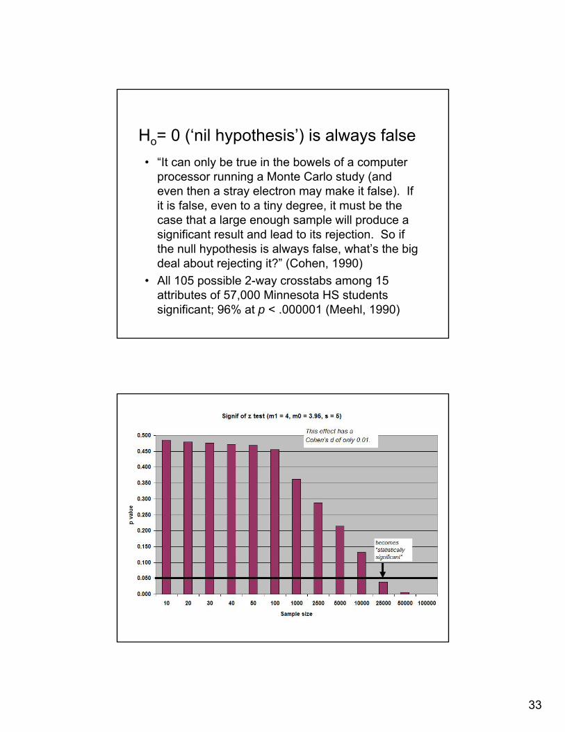
Ho= 0 (‘nil hypothesis’) is always false• “It can only be true in the bowels of a computer

processor running a Monte Carlo study (and even then a stray electron may make it false). If it is false, even to a tiny degree, it must be the case that a large enough sample will produce a significant result and lead to its rejection. So if the null hypothesis is always false, what’s the big deal about rejecting it?” (Cohen, 1990)

• All 105 possible 2-way crosstabs among 15 attributes of 57,000 Minnesota HS students significant; 96% at p < .000001 (Meehl, 1990)

34

Alternatives to sig. testing

• Confidence intervals– avoids dichotomous thinking, highlights

uncertainty– even better if combined with robust statistics,

“bootstrap” standard errors• Bayesian statistical analysis• The prep statistic

The prep statistic

• Killeen (Psy Science, 2005)• Want to know p(d2 >0|d1), where d1 is

observed effect size in earlier study and d2is effect size in next study

• Prep = area under curve of normal probability table up to z = d1/√2σ2

d

35

In praise of prep

• Valid? Calculated as .71, .75, and .79 for 3 meta-analyses where effect was replicated 70%, 74%, and 82% of time

• Requires no assumptions about null hypothesis -- compare psig = p(data|Null is true)

• Easy to communicate: “this effect will replicate 100(prep)% of time”

• But see Geoffrey Iverson et al. (2009a, 2009b) who show that prep is sometimesmisinterpreted, and sometimes too optimistic

Power analysis

• Power (1 - β) = p(Accept H1|H1 true)– power is a function of significance level (α),

sample size (N), and population effect size (ES)

• Cohen suggests conventional level of .80– i.e., .80 : .05 = 4:1 ratio of Type II:Type I errors

• Average power for medium ES, all articles in Journal of Abnormal Psychology– 1960: .46 (Cohen, 1962)

– 1984: .37 (Sedlmeier & Gigerenzer, 1989)

36

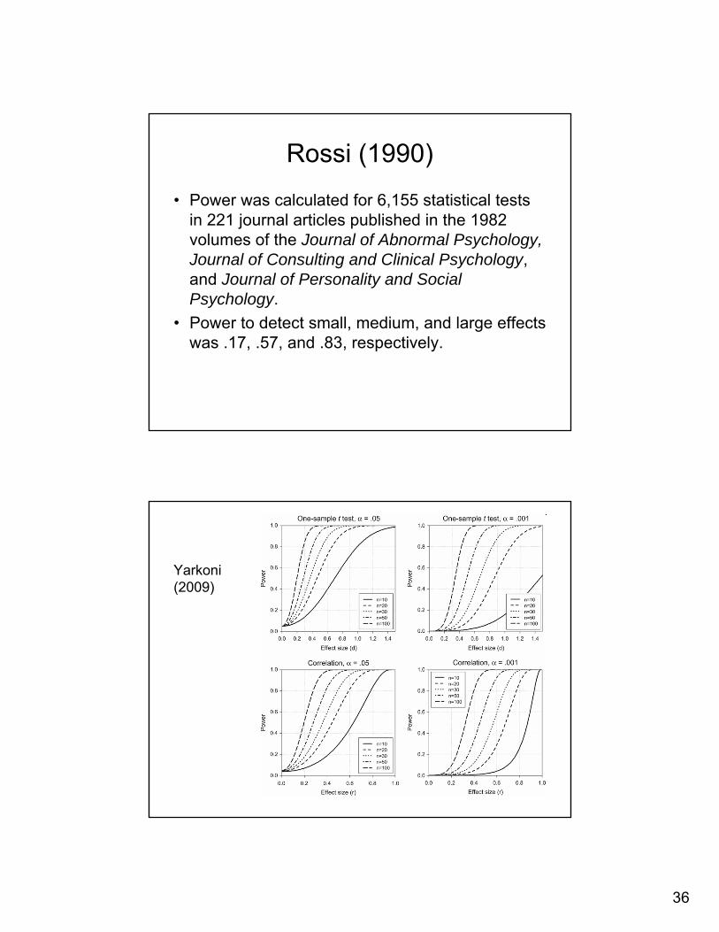
Rossi (1990)

• Power was calculated for 6,155 statistical tests in 221 journal articles published in the 1982 volumes of the Journal of Abnormal Psychology, Journal of Consulting and Clinical Psychology, and Journal of Personality and Social Psychology.

• Power to detect small, medium, and large effects was .17, .57, and .83, respectively.

Yarkoni(2009)

37

“Minimum detectable difference” (MDD) approach

• When trying to determine sample size, “MDD” refers to the smallest effect size you want to detect

– E.g., smallest effect that would be still worth pursuing based on clinical significance or cost-effectiveness

• When N is fixed by real-world constraints, “MDD” refers to the smallest effect size you can detect

– for a given level of power and alpha—usually .8 and .05

Power for 2x2 interaction?• Recall that in a 2x2 factorial experiment, you can

have significant main effects for each variable, and/or a significant interaction effect involving both IVs.

• The power needed to detect a 2x2 interaction effect in a factorial experiment may be the same as the power needed to detect the main effects of the 2 variables. Or you may need more power. It will depend on the nature of the interaction and the degrees of freedom of the test.– For details, see Wahlsten, D. (1991). Sample size to detect a

planned contrast and a one degree-of-freedom interaction effect. Psychological Bulletin, 110, 587-595.

38

Random Assignment of Treatment

Treatment Assignment Group Control Group

Compliers Noncompliers

nonrandomTi = 1 Ti = 0

Intention to Treat (ITT): includes noncompliers in the treatment effect, biasing it downward. But random assignment is preserved.

Random Assignment of Treatment

Treatment Assignment Group Control Group

Compliers

nonrandomTi = 1

Average Treatment Effect on the Treated excludes the non-compliers, so no longer true random assignment. (Threat of selection and attrition biases)

39

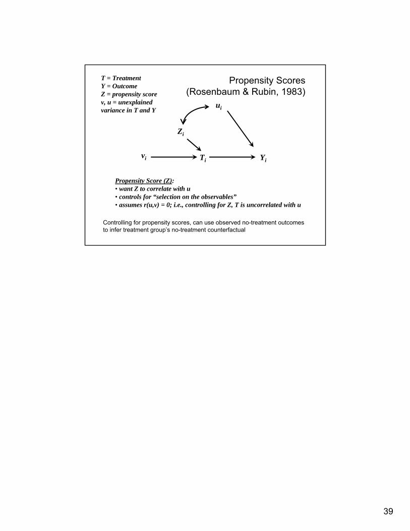
ui

Ti Yivi

Propensity Score (Z):• want Z to correlate with u • controls for “selection on the observables”• assumes r(u,v) = 0; i.e., controlling for Z, T is uncorrelated with u

T = TreatmentY = Outcome Z = propensity scorev, u = unexplained variance in T and Y

Zi

Propensity Scores (Rosenbaum & Rubin, 1983)

Controlling for propensity scores, can use observed no-treatment outcomes to infer treatment group’s no-treatment counterfactual