Experimental design

Experiments vs. observational studies

Manipulative experiments: The only way to proof the causal relationships

BUT

Spatial and temporal limitation of manipulations

Side effects of manipulations

Laboratory, field, natural trajectory (NTE), and natural snapshot experiments (Diamond 1986)

Lab Field NTE NSERegulation ofindep. variables

Highest Medium/low None None

Site matching Highest Medium Medium/low LowestAbility to followtrajectory

Yes Yes Yes No

Maximumtemporal scale

Lowest Lowest Highest Highest

Maximumspatial scale

Lowest Low Highest Highest

Scope (range ofmanipulations)

Lowest Medium/low Medium/high

Highest

Realism None/low High Highest HighestGenerality None Low High High

NTE/NSE - Natural Trajectory/Snapshot Experiment

Observational studies(e.g. for correlation between environment and species, or

estimates of plot characteristics)Random vs. regular sampling plan

Regular design - biased results, when there is some regular structure in the plot (e.g. regular furrows), with the same period as is the distance in the grid - otherwise, better design providing better coverage of the area, and also enables use of special permutation tests.

Manipulative experimentsfrequent trade-off between feasibility and requirements of correct statistical design and power of the tests

To maximize power of the test, you need to maximize number of independent experimental units

For the feasibility and realism, you need plots of some size, to avoid the edge effect

Completely randomized design

Typical analysis: One way ANOVA

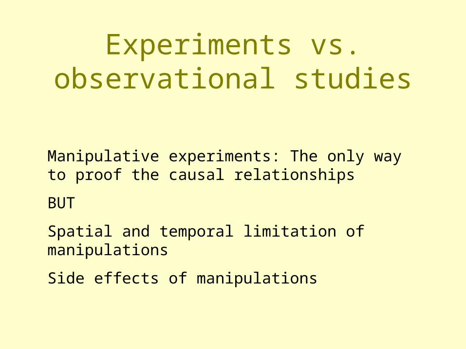
Important - treatments randomly assigned to plots

often, chessboard arrangement or similar regular pattern

E N V I R O N M E N T A L G R A D I E N T

Block 1 Block 2 Block 3 Block 4

Randomized complete blocks

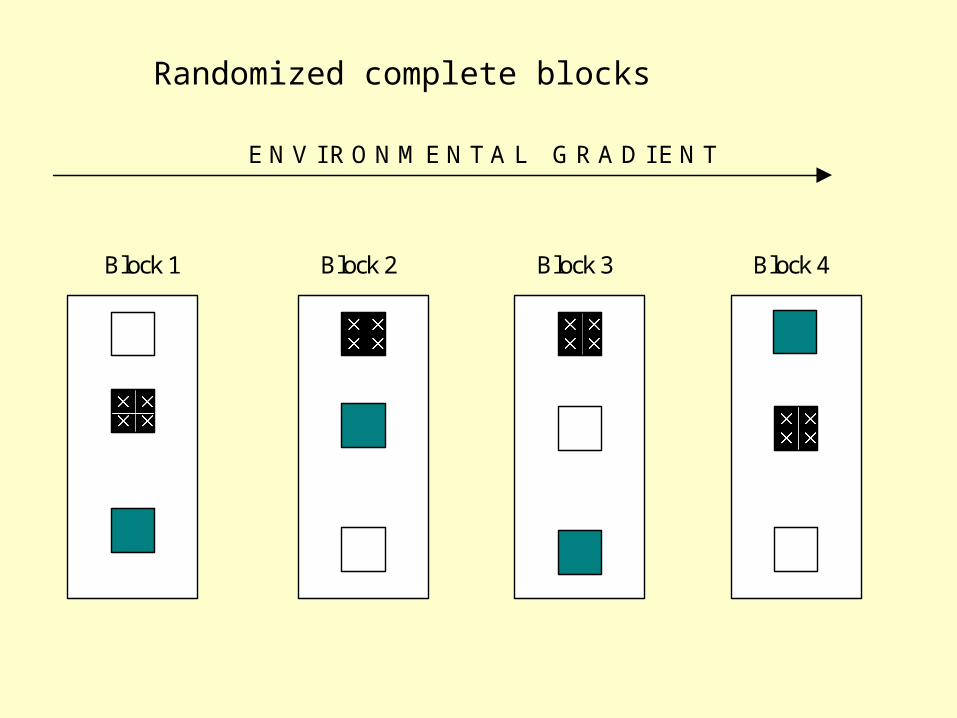
ANOVA, TREAT x BLOCK interaction is error term

TREAT BLOCK RESPO1 RESPO21 1 5 52 1 6 63 1 4 41 2 7 52 2 9 53 2 8 41 3 3 52 3 5 73 3 2 41 4 6 42 4 7 63 4 5 51 5 8 42 5 11 53 5 9 6

TREAT:G_1:1

TREAT:G_2:2

TREAT:G_3:3

BLOCK

RE

SP

O1

0

2

4

6

8

10

12

G_1:1 G_2:2 G_3:3 G_4:4 G_5:5

If the block has strong explanatory power, the RCB design is stronger

df MS df MSEffect Effect Error Error F p-level

TREAT 2 6.066667 8 0.4 15.16667 0.001897BLOCK 4 17 8 0.4 42.5 1.97E-05

TREAT 2 6.066667 12 5.933333 1.022472 0.389016

TREAT:G_1:1

TREAT:G_2:2

TREAT:G_3:3

BLOCK

RE

SP

O2

3.5

4.0

4.5

5.0

5.5

6.0

6.5

7.0

7.5

G_1:1 G_2:2 G_3:3 G_4:4 G_5:5

df MS df MSEffect Effect Error Error F p-level

TREAT 2 2.4 8 0.816667 2.938776 0.110435BLOCK 4 0.166667 8 0.816667 0.204082 0.929067

TREAT 2 2.4 12 0.6 4 0.046656

If the block has no explanatory power, the RCB design is weak

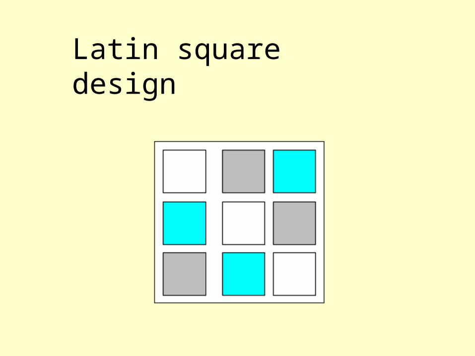
Latin square design

Most frequent errors - pseudoreplications

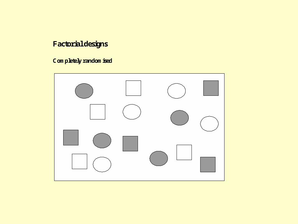
Factorial designs

Completely randomised

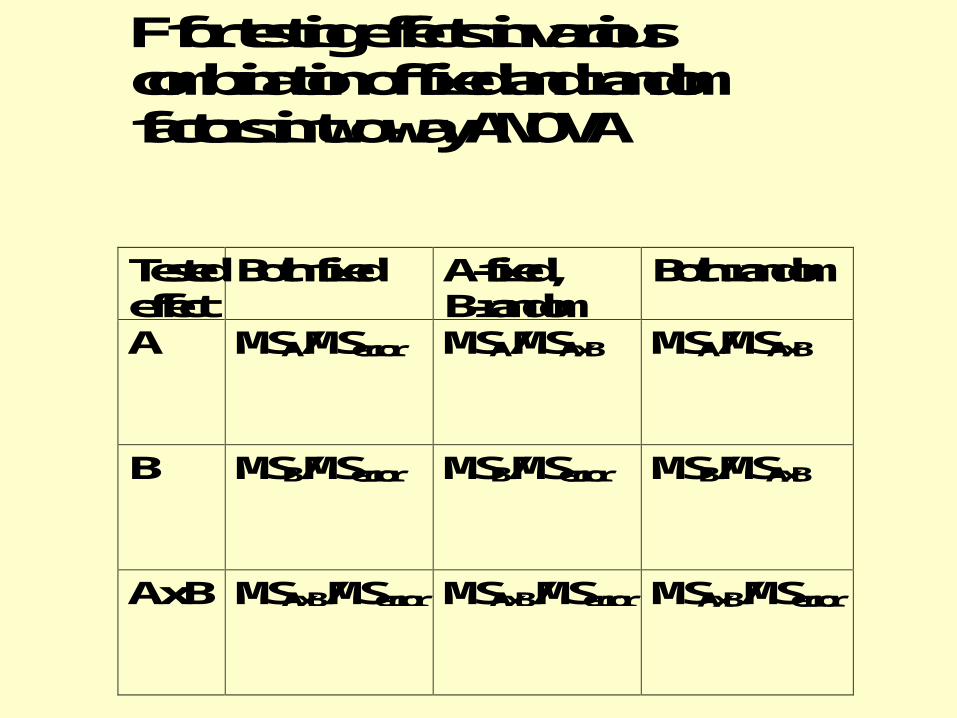
F for testing effects in variouscombination of fixed and randomfactors in two-way ANOVA

Testedeffect

Both fixed A-fixed,B-random

Both random

A MSA/MSerror MSA/MSAxB MSA/MSAxB

B MSB/MSerror MSB/MSerror MSB/MSAxB

A x B MSAxB/MSerror MSAxB/MSerror MSAxB/MSerror

COUNTRY FERTIL NOSPEC1 CZ 0.000 9.0002 CZ 0.000 8.0003 CZ 0.000 6.0004 CZ 1.000 4.0005 CZ 1.000 5.0006 CZ 1.000 4.0007 UK 0.000 11.0008 UK 0.000 12.0009 UK 0.000 10.00010 UK 1.000 3.00011 UK 1.000 4.00012 UK 1.000 3.00013 NL 0.000 5.00014 NL 0.000 6.00015 NL 0.000 7.00016 NL 1.000 6.00017 NL 1.000 6.00018 NL 1.000 8.000

Fertilization experiment in three countries

Summary of all Effects; design: (new.sta)1-COUNTRY, 2-FERTIL

df MS df MS Effect Effect Error Error F p-level

1 2 2.16667 12 1.05556 2.05263 .1711122 1 53.38889 2 26.05556 2.04904 .28862412 2 26.05556 12 1.05556 24.68421 .000056

Summary of all Effects; design: (new.sta)1-COUNTRY, 2-FERTIL

df MS df MS Effect Effect Error Error F p-level

1 2 2.16667 12 1.055556 2.05263 .1711122 1 53.38889 12 1.055556 50.57895 .00001212 2 26.05556 12 1.055556 24.68421 .000056

Country is a fixed factor (i.e., we are interested in the three plots only)

Country is a random factor (i.e., the three plots arew considered as random selection of all plots of this type in Europe - [to make Brussels happy])

Nested designs („split-plot“)

Two explanatory variables, Treatment and Plot,

Plot is random factor nested in Treatment.

Accordingly, there are two error terms, effect of Treatment is tested against Plot, effect of Plot against residual variability:

F(Treat)=MS(Treat)/MS(Plot)

F(Plot)=MS(Plot)/MS(Resid) [often not of interest]

Plot 1 Plot 2 Plot 3

Plot 4 Plot 5 Plot 6

C

P

N

N

P

C

C

N

P

N

CP C

N

P N

P

C

Split plot (main plots and split plots - two error levels)

df MS df MSEffect Effect Error Error F p-level

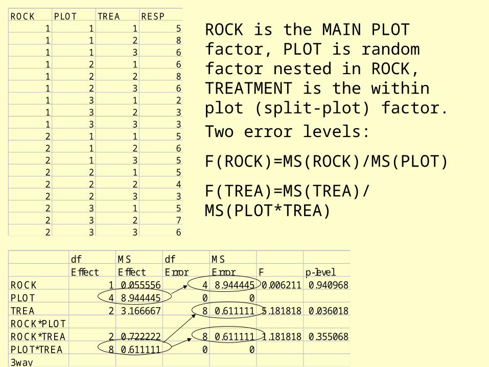
ROCK 1 0.055556 4 8.944445 0.006211 0.940968PLOT 4 8.944445 0 0TREA 2 3.166667 8 0.611111 5.181818 0.036018ROCK*PLOTROCK*TREA 2 0.722222 8 0.611111 1.181818 0.355068PLOT*TREA 8 0.611111 0 03way

ROCK PLOT TREA RESP1 1 1 51 1 2 81 1 3 61 2 1 61 2 2 81 2 3 61 3 1 21 3 2 31 3 3 32 1 1 52 1 2 62 1 3 52 2 1 52 2 2 42 2 3 32 3 1 52 3 2 72 3 3 6

ROCK is the MAIN PLOT factor, PLOT is random factor nested in ROCK, TREATMENT is the within plot (split-plot) factor.

Two error levels:

F(ROCK)=MS(ROCK)/MS(PLOT)

F(TREA)=MS(TREA)/MS(PLOT*TREA)

Following changes in time

Non-replicated BACI (Before-after-control-impact)

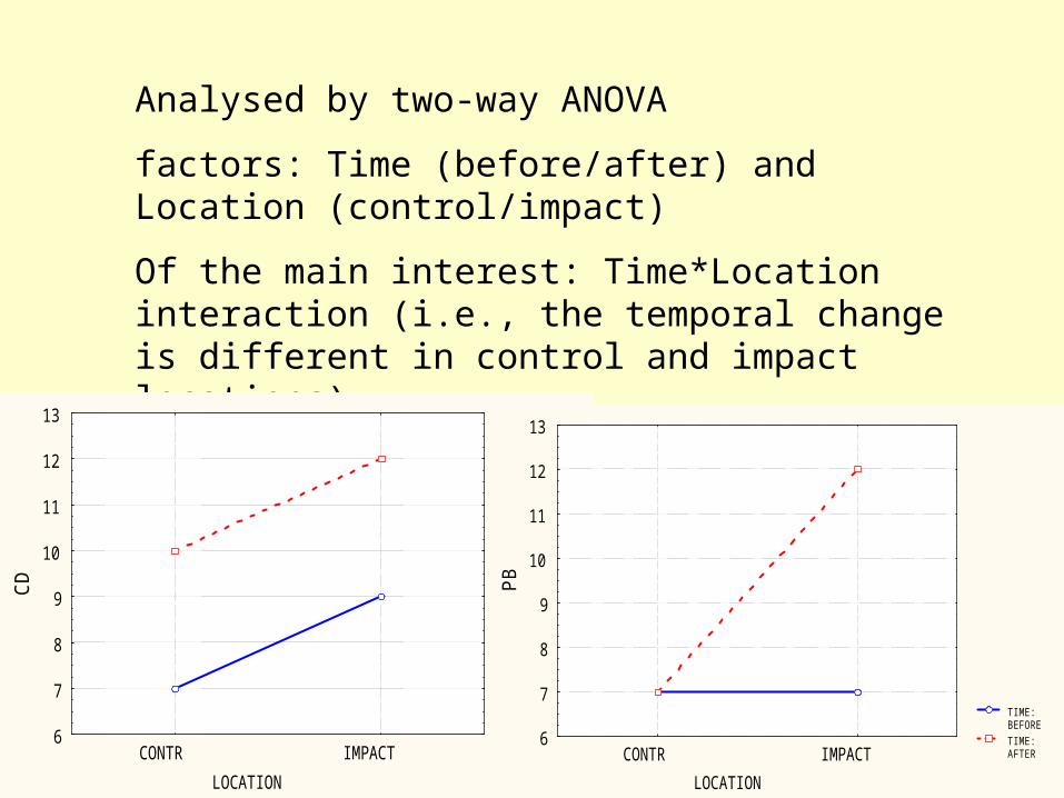
Analysed by two-way ANOVA

factors: Time (before/after) and Location (control/impact)

Of the main interest: Time*Location interaction (i.e., the temporal change is different in control and impact locations)

TIME:BEFORE

TIME:AFTER

LOCATION

CD

6

7

8

9

10

11

12

13

CONTR IMPACT

TIME:BEFORE

TIME:AFTER

LOCATION

PB

6

7

8

9

10

11

12

13

CONTR IMPACT

In fact, in non-replicated BACI, the test is based on pseudoreplications.

Should NOT be used in experimental setups

In impact assessments, often the best possibility

(The best need not be always good enough.)

T0 Treatment T1 T2

Control

Control

Control

Impact

Impact

Impact

Replicated BACI - repeated measurements

Usually analysed by “univariate repeated measures ANOVA”. This is in fact split-plot, where TREATment is the main-plot effect, time is the within-plot effect, individuals (or experimental units) and nested within a treatment.

Of the main interest is interaction TIME*TREAT

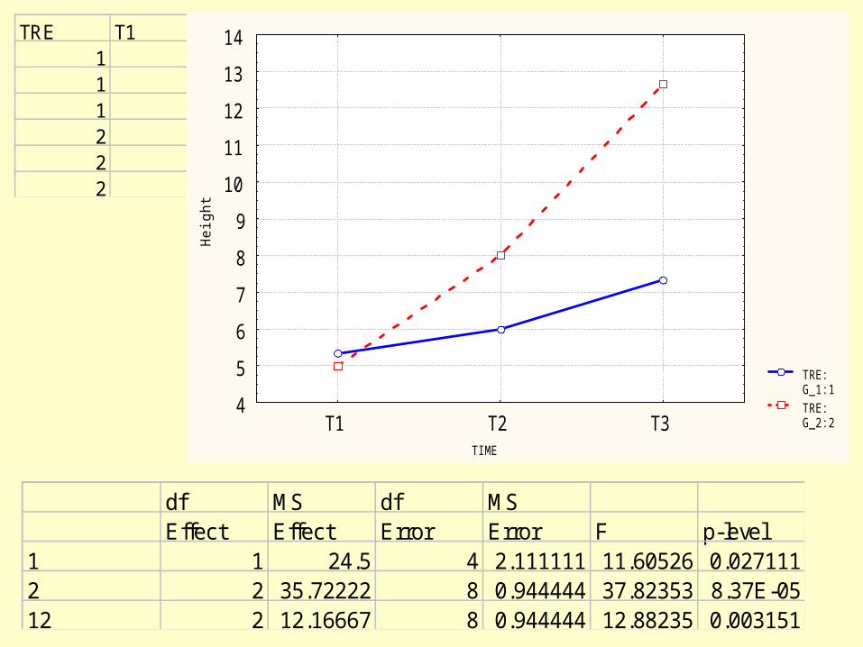
df MS df MSEffect Effect Error Error F p-level

1 1 24.5 4 2.111111 11.60526 0.0271112 2 35.72222 8 0.944444 37.82353 8.37E-0512 2 12.16667 8 0.944444 12.88235 0.003151

TRE T1 T2 T31 5 6 71 6 5 81 5 7 72 4 7 112 6 8 122 5 9 15

TRE:G_1:1

TRE:G_2:2

TIME

He

igh

t

4

5

6

7

8

9

10

11

12

13

14

T1 T2 T3