Embed Size (px)
Citation preview

Experimental design and statistical analyses of data
Lesson 4:
Analysis of variance II
A posteriori tests
Model control
How to choose the best model
Growth of bean plants in four different media
Zn Cu Mn Control Overall
Biomass (y)
61.7
59.4
60.5
59.2
57.6
57.0
58.4
57.3
57.8
59.9
62.3
66.2
65.2
63.7
64.1
58.1
56.3
58.9
57.4
56.1
ni 5
59.7
2.35
5
58.1
1.33
5
64.3
2.20
5
57.4
1.43
20
59.86
9.207
Completely randomized design (one-way anova)
iy2is
3322110 xxxy

How to do it with SAS
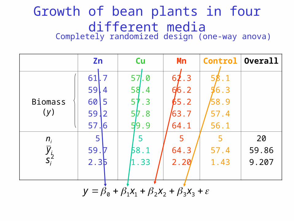
DATA medium;
/* 20 bean plants exposed to 4 different treatments
(5 plants per treatment)
Mn = extra mangan added to the soil
Zn = ekstra zink added to the soil
Cu = ekstra cupper added to the soil
K = control soil
The dependent variable (Mass) is the biomass of the plants at harvest */
INPUT treat $ mass ;
/* treat = treatment */
/* mass = biomass of a plant */
CARDS;
zn 61.7
zn 59.4
zn 60.5
zn 59.2
zn 57.6
cu 57.0
cu 58.4
cu 57.3
cu 57.8
cu 59.9
mn 62.3
mn 66.2
mn 65.2
mn 63.7
mn 64.1
k 58.1
k 56.3
k 58.9
k 57.4
k 56.1
;
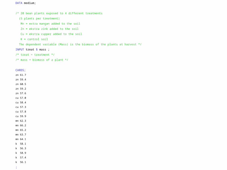
PROC SORT; /* sort the observations according
to treatment */
BY treat;
RUN;
/* compute average and 95% confidence limits for each treatment */
PROC MEANS N MEAN CLM;
BY treat;
RUN;
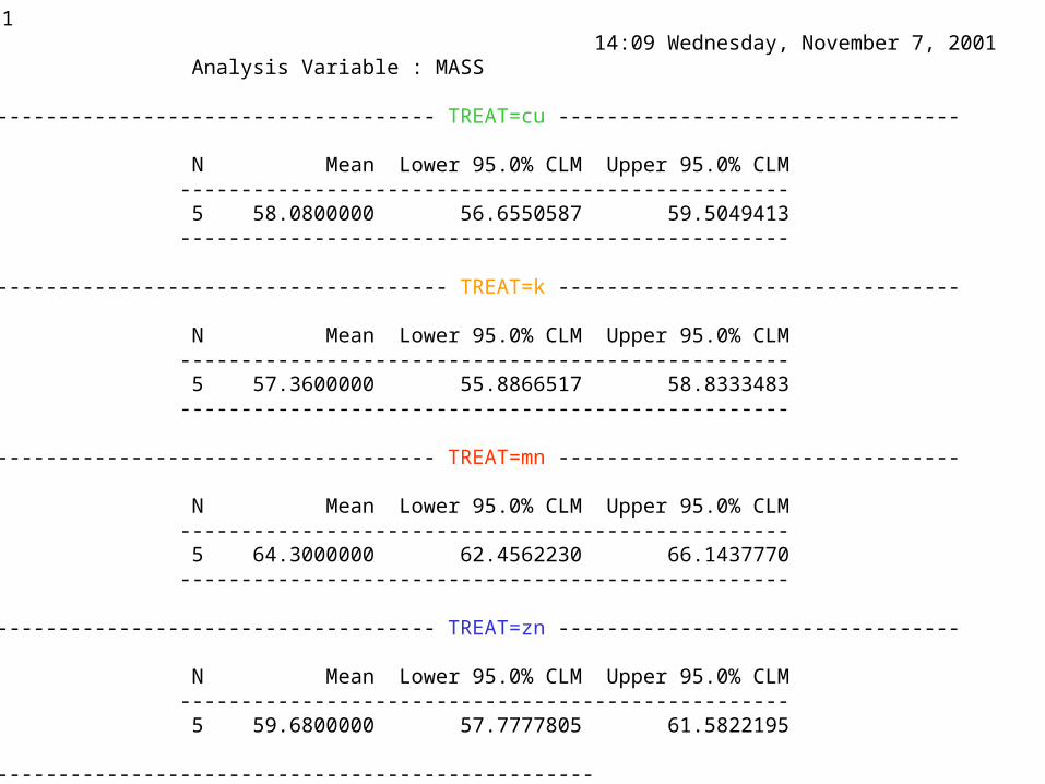
1 14:09 Wednesday, November 7, 2001 Analysis Variable : MASS ------------------------------------- TREAT=cu --------------------------------- N Mean Lower 95.0% CLM Upper 95.0% CLM -------------------------------------------------- 5 58.0800000 56.6550587 59.5049413 -------------------------------------------------- -------------------------------------- TREAT=k --------------------------------- N Mean Lower 95.0% CLM Upper 95.0% CLM -------------------------------------------------- 5 57.3600000 55.8866517 58.8333483 -------------------------------------------------- ------------------------------------- TREAT=mn --------------------------------- N Mean Lower 95.0% CLM Upper 95.0% CLM -------------------------------------------------- 5 64.3000000 62.4562230 66.1437770 -------------------------------------------------- ------------------------------------- TREAT=zn --------------------------------- N Mean Lower 95.0% CLM Upper 95.0% CLM -------------------------------------------------- 5 59.6800000 57.7777805 61.5822195 --------------------------------------------------
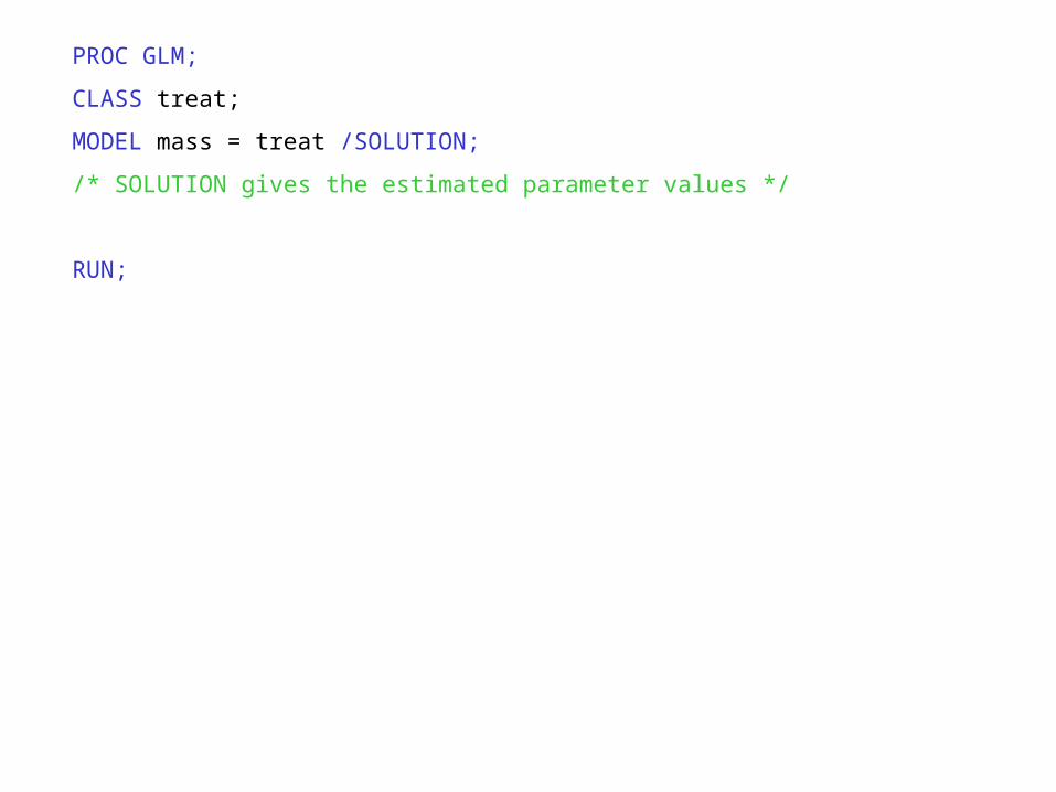
PROC GLM;
CLASS treat;
MODEL mass = treat /SOLUTION;
/* SOLUTION gives the estimated parameter values */
RUN;
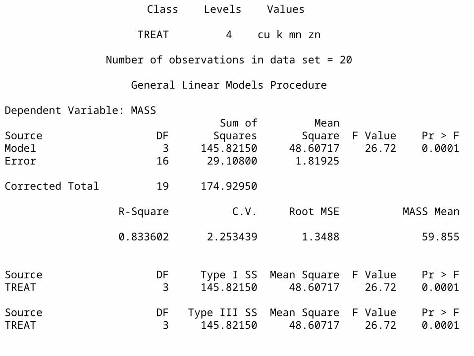
Class Levels Values TREAT 4 cu k mn zn Number of observations in data set = 20 General Linear Models Procedure Dependent Variable: MASS Sum of MeanSource DF Squares Square F Value Pr > FModel 3 145.82150 48.60717 26.72 0.0001Error 16 29.10800 1.81925 Corrected Total 19 174.92950 R-Square C.V. Root MSE MASS Mean 0.833602 2.253439 1.3488 59.855 Source DF Type I SS Mean Square F Value Pr > FTREAT 3 145.82150 48.60717 26.72 0.0001 Source DF Type III SS Mean Square F Value Pr > FTREAT 3 145.82150 48.60717 26.72 0.0001
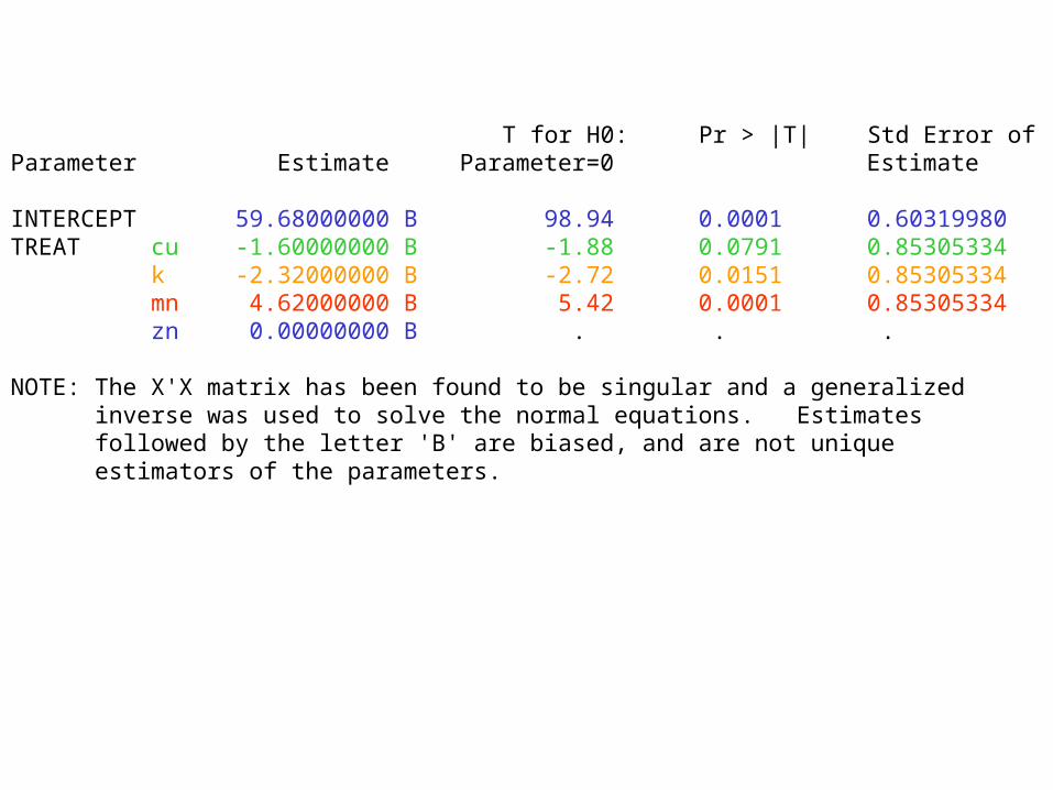
T for H0: Pr > |T| Std Error ofParameter Estimate Parameter=0 Estimate INTERCEPT 59.68000000 B 98.94 0.0001 0.60319980TREAT cu -1.60000000 B -1.88 0.0791 0.85305334 k -2.32000000 B -2.72 0.0151 0.85305334 mn 4.62000000 B 5.42 0.0001 0.85305334 zn 0.00000000 B . . . NOTE: The X'X matrix has been found to be singular and a generalized inverse was used to solve the normal equations. Estimates followed by the letter 'B' are biased, and are not unique estimators of the parameters.
PROC GLM;
CLASS treat;
MODEL mass = treat /SOLUTION;
/* SOLUTION gives the estimated parameter values */
/*Test for pairwise differences between treatments by
linear contrasts */
CONTRAST 'Cu vs K' Treat 1 -1 0 0;
CONTRAST 'Cu vs Mn' Treat 1 0 -1 0;
CONTRAST 'Cu vs Zn' Treat 1 0 0 -1;
CONTRAST 'K vs Mn' Treat 0 1 -1 0;
CONTRAST 'K vs Zn' Treat 0 1 0 -1;
CONTRAST 'Mn vs Zn' Treat 0 0 1 -1;
/* test for whether the 3 treatments with added minerals are different from the control */
CONTRAST 'K vs Cu, Mn Zn' Treat 1 -3 1 1;
RUN;
Contrast DF Contrast SS Mean Square F Value Pr > F Cu vs K 1 1.29600 1.29600 0.71 0.4111Cu vs Mn 1 96.72100 96.72100 53.17 0.0001Cu vs Zn 1 6.40000 6.40000 3.52 0.0791K vs Mn 1 120.40900 120.40900 66.19 0.0001K vs Zn 1 13.45600 13.45600 7.40 0.0151Mn vs Zn 1 53.36100 53.36100 29.33 0.0001K vs Cu, Mn Zn 1 41.50017 41.50017 22.81 0.0002
PROC GLM;
CLASS treat;
MODEL mass = treat /SOLUTION;
/* SOLUTION gives the estimated parameter values */
/* Test for differences between levels of treatment */
MEANS treat / BON DUNCAN SCHEFFE TUKEY DUNNETT('k');
RUN;
Tukey's Studentized Range (HSD) Test for variable: MASS NOTE: This test controls the type I experimentwise error rate. Alpha= 0.05 Confidence= 0.95 df= 16 MSE= 1.81925 Critical Value of Studentized Range= 4.046 Minimum Significant Difference= 2.4406 Comparisons significant at the 0.05 level are indicated by '***'. Simultaneous Simultaneous Lower Difference Upper TREAT Confidence Between Confidence Comparison Limit Means Limit mn - zn 2.1794 4.6200 7.0606 *** mn - cu 3.7794 6.2200 8.6606 *** mn - k 4.4994 6.9400 9.3806 *** zn - mn -7.0606 -4.6200 -2.1794 *** zn - cu -0.8406 1.6000 4.0406 zn - k -0.1206 2.3200 4.7606 cu - mn -8.6606 -6.2200 -3.7794 *** cu - zn -4.0406 -1.6000 0.8406 cu - k -1.7206 0.7200 3.1606 k - mn -9.3806 -6.9400 -4.4994 *** k - zn -4.7606 -2.3200 0.1206 k - cu -3.1606 -0.7200 1.7206
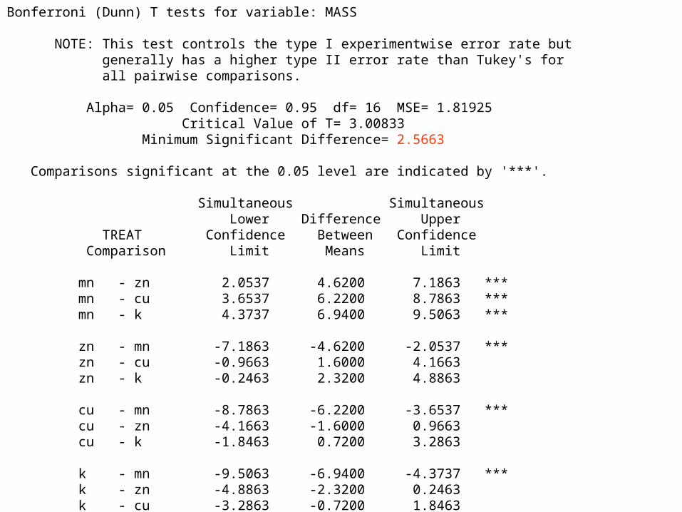
Bonferroni (Dunn) T tests for variable: MASS NOTE: This test controls the type I experimentwise error rate but generally has a higher type II error rate than Tukey's for all pairwise comparisons. Alpha= 0.05 Confidence= 0.95 df= 16 MSE= 1.81925 Critical Value of T= 3.00833 Minimum Significant Difference= 2.5663 Comparisons significant at the 0.05 level are indicated by '***'. Simultaneous Simultaneous Lower Difference Upper TREAT Confidence Between Confidence Comparison Limit Means Limit mn - zn 2.0537 4.6200 7.1863 *** mn - cu 3.6537 6.2200 8.7863 *** mn - k 4.3737 6.9400 9.5063 *** zn - mn -7.1863 -4.6200 -2.0537 *** zn - cu -0.9663 1.6000 4.1663 zn - k -0.2463 2.3200 4.8863 cu - mn -8.7863 -6.2200 -3.6537 *** cu - zn -4.1663 -1.6000 0.9663 cu - k -1.8463 0.7200 3.2863 k - mn -9.5063 -6.9400 -4.3737 *** k - zn -4.8863 -2.3200 0.2463 k - cu -3.2863 -0.7200 1.8463
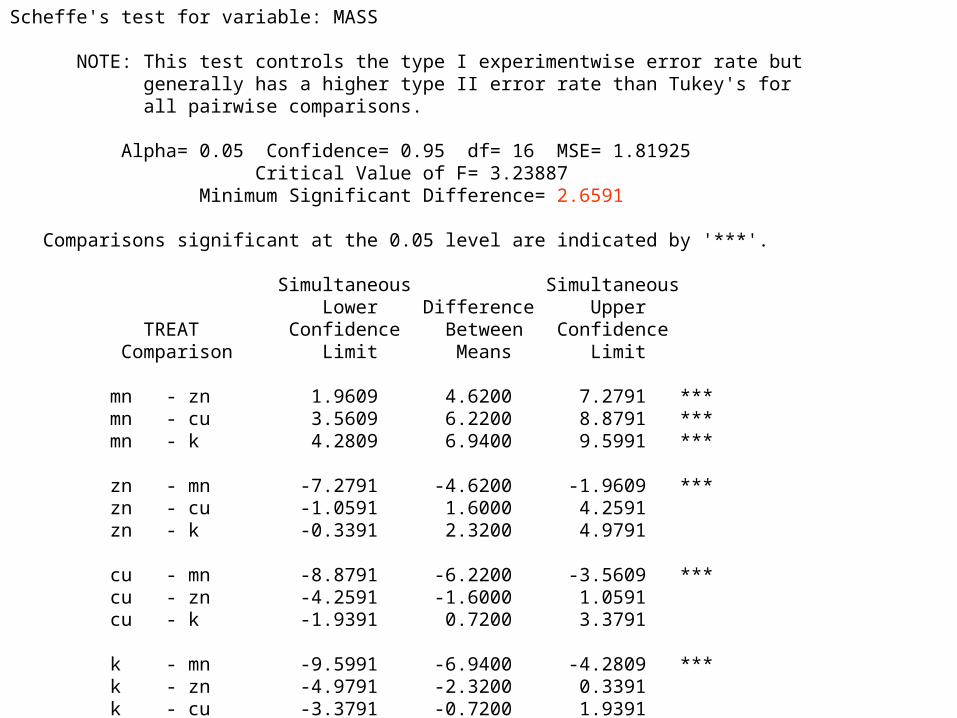
Scheffe's test for variable: MASS NOTE: This test controls the type I experimentwise error rate but generally has a higher type II error rate than Tukey's for all pairwise comparisons. Alpha= 0.05 Confidence= 0.95 df= 16 MSE= 1.81925 Critical Value of F= 3.23887 Minimum Significant Difference= 2.6591 Comparisons significant at the 0.05 level are indicated by '***'. Simultaneous Simultaneous Lower Difference Upper TREAT Confidence Between Confidence Comparison Limit Means Limit mn - zn 1.9609 4.6200 7.2791 *** mn - cu 3.5609 6.2200 8.8791 *** mn - k 4.2809 6.9400 9.5991 *** zn - mn -7.2791 -4.6200 -1.9609 *** zn - cu -1.0591 1.6000 4.2591 zn - k -0.3391 2.3200 4.9791 cu - mn -8.8791 -6.2200 -3.5609 *** cu - zn -4.2591 -1.6000 1.0591 cu - k -1.9391 0.7200 3.3791 k - mn -9.5991 -6.9400 -4.2809 *** k - zn -4.9791 -2.3200 0.3391 k - cu -3.3791 -0.7200 1.9391
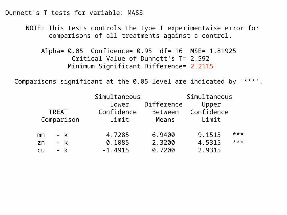
Dunnett's T tests for variable: MASS NOTE: This tests controls the type I experimentwise error for comparisons of all treatments against a control. Alpha= 0.05 Confidence= 0.95 df= 16 MSE= 1.81925 Critical Value of Dunnett's T= 2.592 Minimum Significant Difference= 2.2115 Comparisons significant at the 0.05 level are indicated by '***'. Simultaneous Simultaneous Lower Difference Upper TREAT Confidence Between Confidence Comparison Limit Means Limit mn - k 4.7285 6.9400 9.1515 *** zn - k 0.1085 2.3200 4.5315 *** cu - k -1.4915 0.7200 2.9315
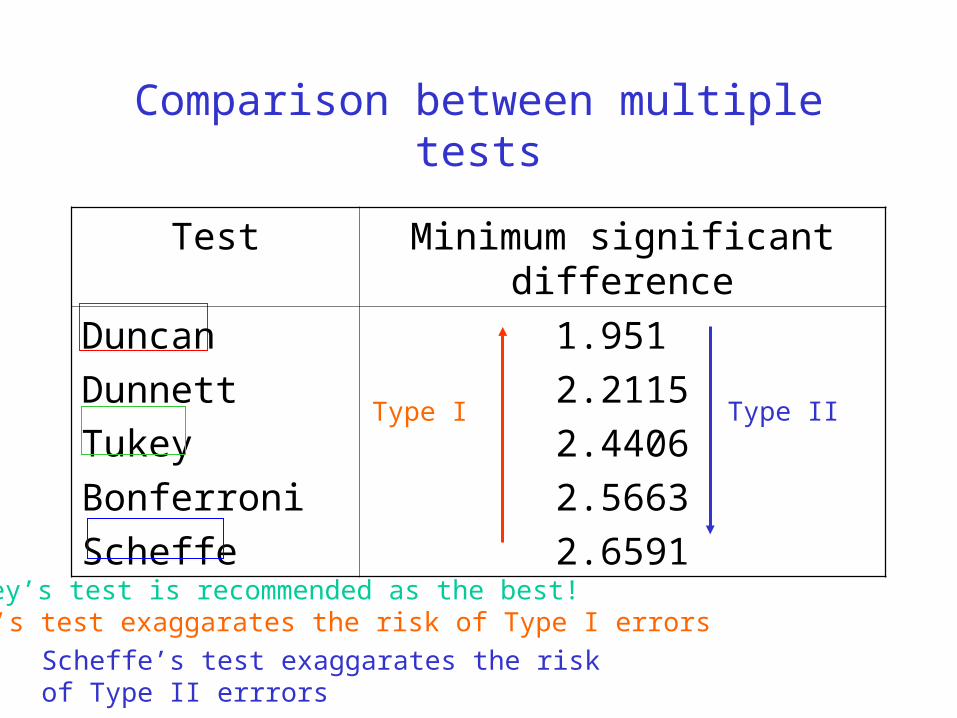
Duncan’s test exaggarates the risk of Type I errors
Comparison between multiple tests
Test Minimum significant difference
Duncan
Dunnett
Tukey
Bonferroni
Scheffe
1.951
2.2115
2.4406
2.5663
2.6591
Type I
Scheffe’s test exaggarates the risk of Type II errrors
Type II
Tukey’s test is recommended as the best!
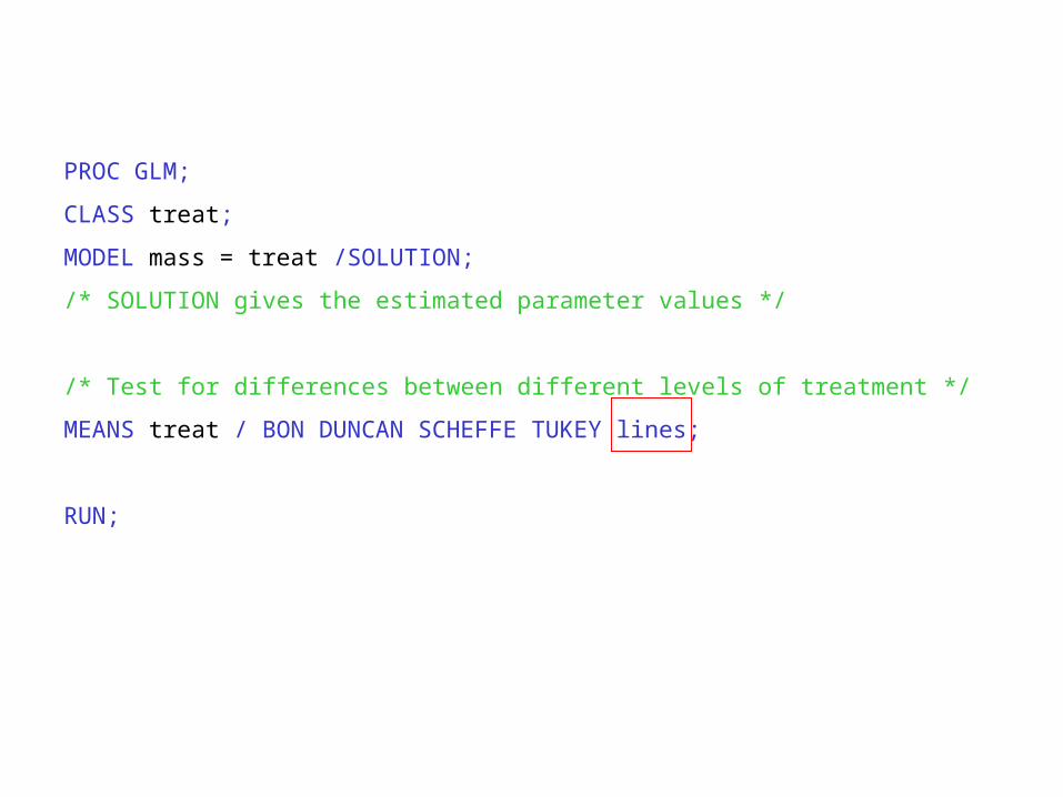
PROC GLM;
CLASS treat;
MODEL mass = treat /SOLUTION;
/* SOLUTION gives the estimated parameter values */
/* Test for differences between different levels of treatment */
MEANS treat / BON DUNCAN SCHEFFE TUKEY lines;
RUN;
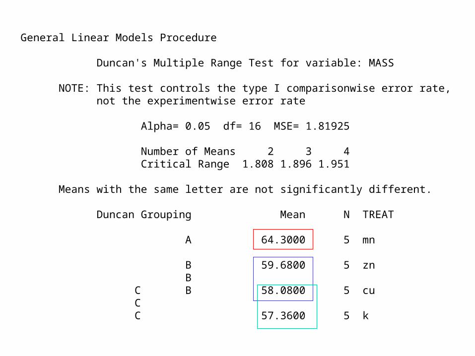
General Linear Models Procedure Duncan's Multiple Range Test for variable: MASS NOTE: This test controls the type I comparisonwise error rate, not the experimentwise error rate Alpha= 0.05 df= 16 MSE= 1.81925 Number of Means 2 3 4 Critical Range 1.808 1.896 1.951 Means with the same letter are not significantly different. Duncan Grouping Mean N TREAT A 64.3000 5 mn B 59.6800 5 zn B C B 58.0800 5 cu C C 57.3600 5 k
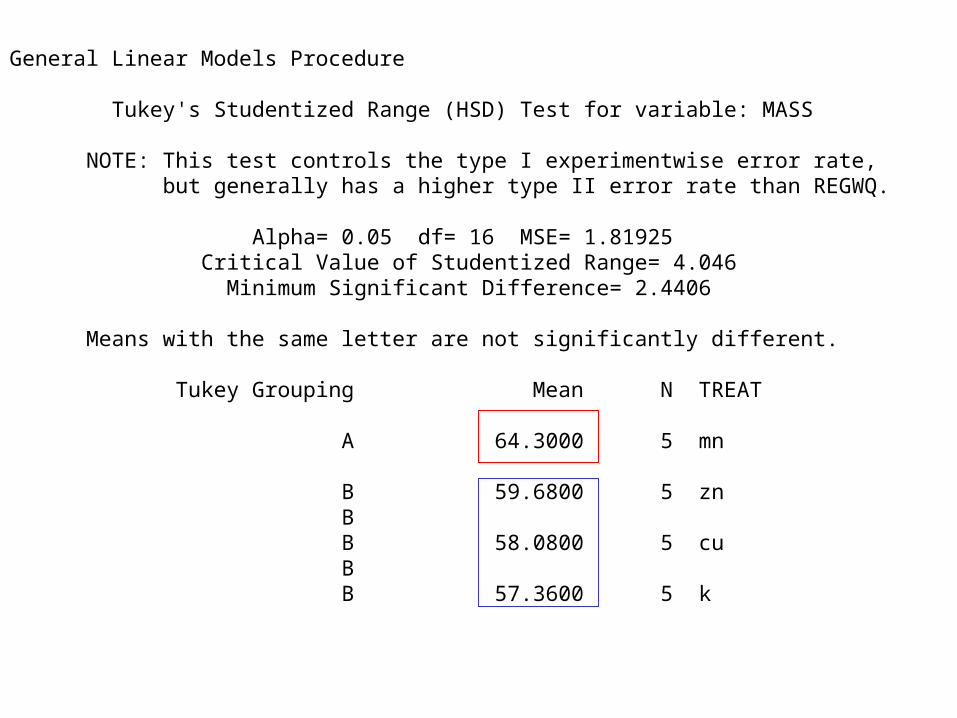
General Linear Models Procedure Tukey's Studentized Range (HSD) Test for variable: MASS NOTE: This test controls the type I experimentwise error rate, but generally has a higher type II error rate than REGWQ. Alpha= 0.05 df= 16 MSE= 1.81925 Critical Value of Studentized Range= 4.046 Minimum Significant Difference= 2.4406 Means with the same letter are not significantly different. Tukey Grouping Mean N TREAT A 64.3000 5 mn B 59.6800 5 zn B B 58.0800 5 cu B B 57.3600 5 k
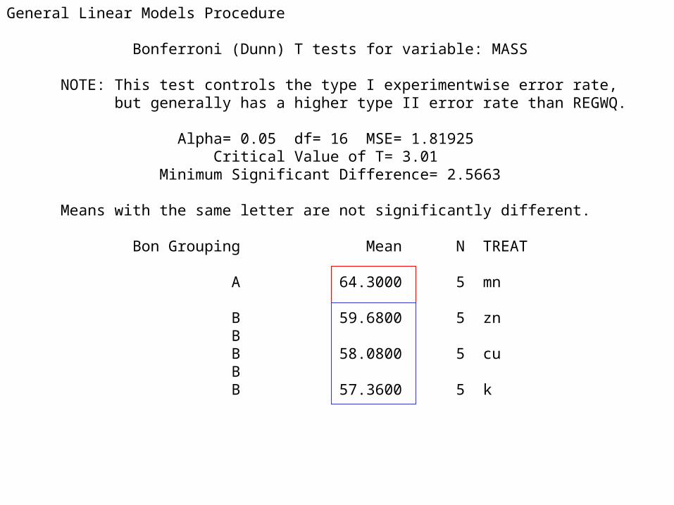
General Linear Models Procedure Bonferroni (Dunn) T tests for variable: MASS NOTE: This test controls the type I experimentwise error rate, but generally has a higher type II error rate than REGWQ. Alpha= 0.05 df= 16 MSE= 1.81925 Critical Value of T= 3.01 Minimum Significant Difference= 2.5663 Means with the same letter are not significantly different. Bon Grouping Mean N TREAT A 64.3000 5 mn B 59.6800 5 zn B B 58.0800 5 cu B B 57.3600 5 k
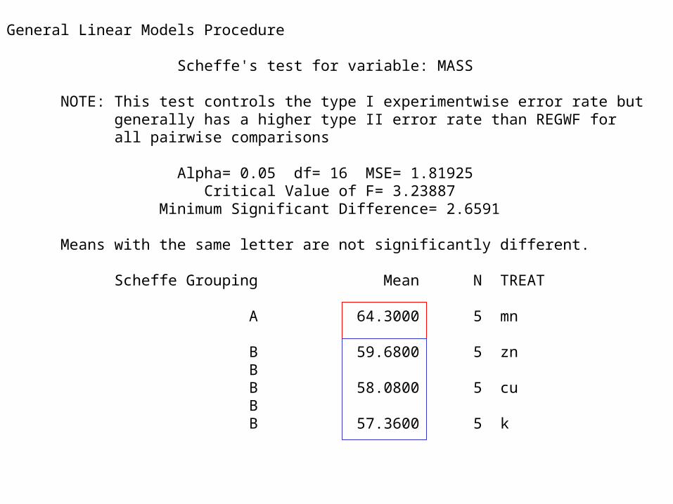
General Linear Models Procedure Scheffe's test for variable: MASS NOTE: This test controls the type I experimentwise error rate but generally has a higher type II error rate than REGWF for all pairwise comparisons Alpha= 0.05 df= 16 MSE= 1.81925 Critical Value of F= 3.23887 Minimum Significant Difference= 2.6591 Means with the same letter are not significantly different. Scheffe Grouping Mean N TREAT A 64.3000 5 mn B 59.6800 5 zn B B 58.0800 5 cu B B 57.3600 5 k
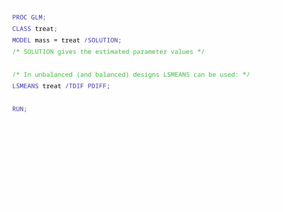
PROC GLM;
CLASS treat;
MODEL mass = treat /SOLUTION;
/* SOLUTION gives the estimated parameter values */
/* In unbalanced (and balanced) designs LSMEANS can be used: */
LSMEANS treat /TDIF PDIFF;
RUN;
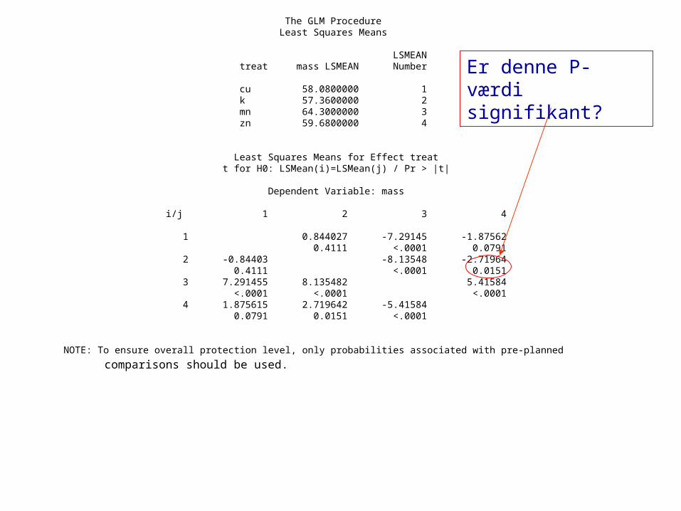
The GLM Procedure Least Squares Means LSMEAN treat mass LSMEAN Number cu 58.0800000 1 k 57.3600000 2 mn 64.3000000 3 zn 59.6800000 4 Least Squares Means for Effect treat t for H0: LSMean(i)=LSMean(j) / Pr > |t| Dependent Variable: mass i/j 1 2 3 4 1 0.844027 -7.29145 -1.87562 0.4111 <.0001 0.0791 2 -0.84403 -8.13548 -2.71964 0.4111 <.0001 0.0151 3 7.291455 8.135482 5.41584 <.0001 <.0001 <.0001 4 1.875615 2.719642 -5.41584 0.0791 0.0151 <.0001 NOTE: To ensure overall protection level, only probabilities associated with pre-planned
comparisons should be used.
Er denne P-værdi signifikant?
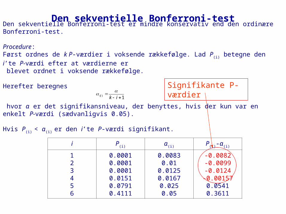
Den sekventielle Bonferroni-testDen sekventielle Bonferroni-test er mindre konservativ end den ordinære Bonferroni-test. Procedure:Først ordnes de k P-værdier i voksende rækkefølge. Lad P(i) betegne den i’te P-værdi efter at værdierne er
blevet ordnet i voksende rækkefølge. Herefter beregnes
1)(
iki
hvor α er det signifikansniveau, der benyttes, hvis der kun var en enkelt P-værdi (sædvanligvis 0.05). Hvis P(i) < α(i) er den i’te P-værdi signifikant.
i P(i) α(i) P(i)-α(i)
123456
0.00010.00010.00010.01510.07910.4111
0.00830.01
0.01250.01670.0250.05
-0.0082-0.0099-0.0124
-0.001570.05410.3611
Signifikante P-værdier
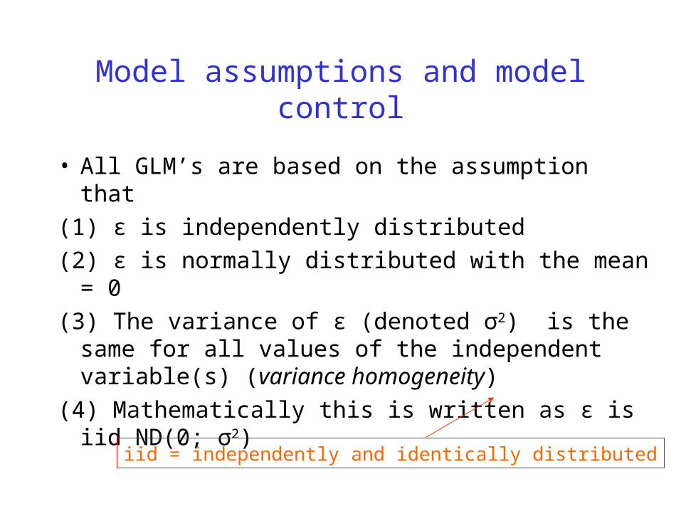
Model assumptions and model control
• All GLM’s are based on the assumption that
(1) ε is independently distributed
(2) ε is normally distributed with the mean = 0
(3) The variance of ε (denoted σ2) is the same for all values of the independent variable(s) (variance homogeneity)
(4) Mathematically this is written as ε is iid ND(0; σ2)
iid = independently and identically distributed
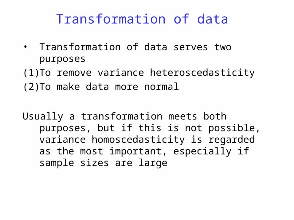
Transformation of data
• Transformation of data serves two purposes
(1) To remove variance heteroscedasticity
(2) To make data more normal
Usually a transformation meets both purposes, but if this is not possible, variance homoscedasticity is regarded as the most important, especially if sample sizes are large

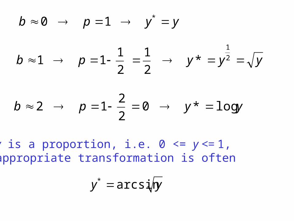
How to choose the appropriate transformation?
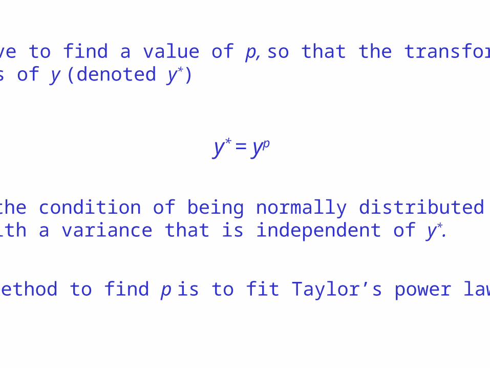
y* = yp
We have to find a value of p, so that the transformedvalues of y (denoted y*)
meet the condition of being normally distributedand with a variance that is independent of y*.
A useful method to find p is to fit Taylor’s power law to data
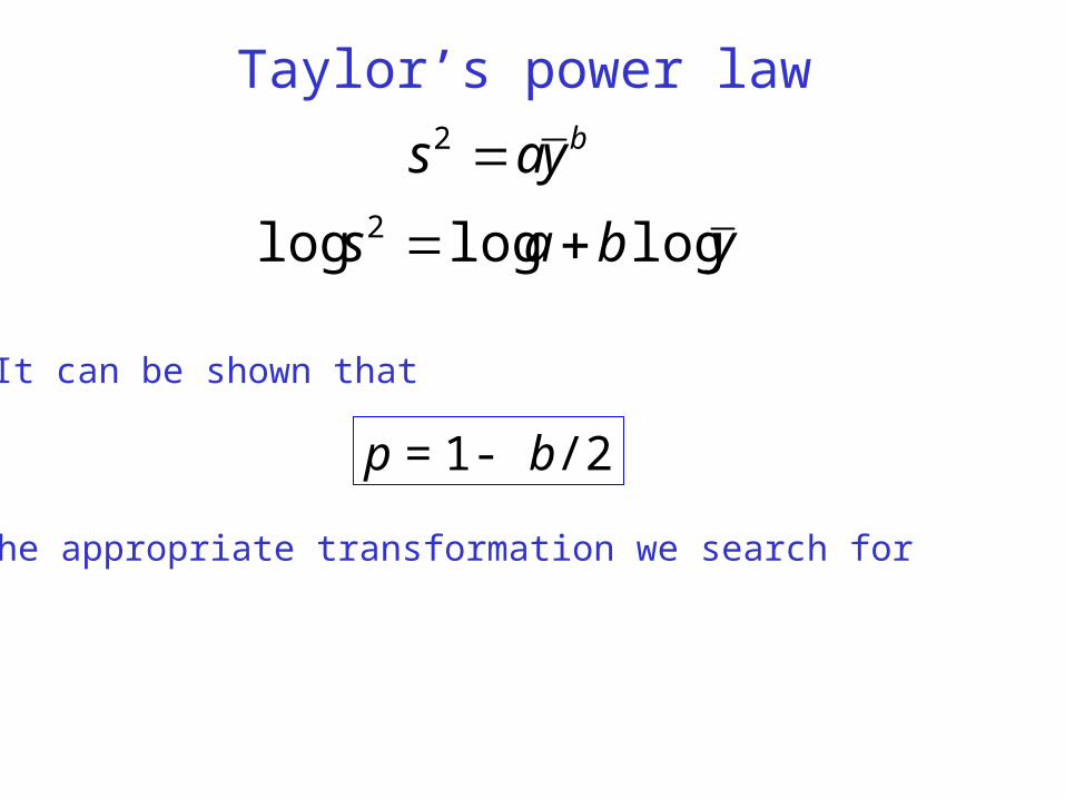
Taylor’s power lawbyas 2
It can be shown that
p = 1- b/2
is the appropriate transformation we search for
ybas logloglog 2
yyypb 2
1
*2
1
2
111
yypb log*02
212
yypb *10
If y is a proportion, i.e. 0 <= y <= 1, an appropriate transformation is often
yy arcsin*
10-02
10-01
1000
1001
1002
1003
1004
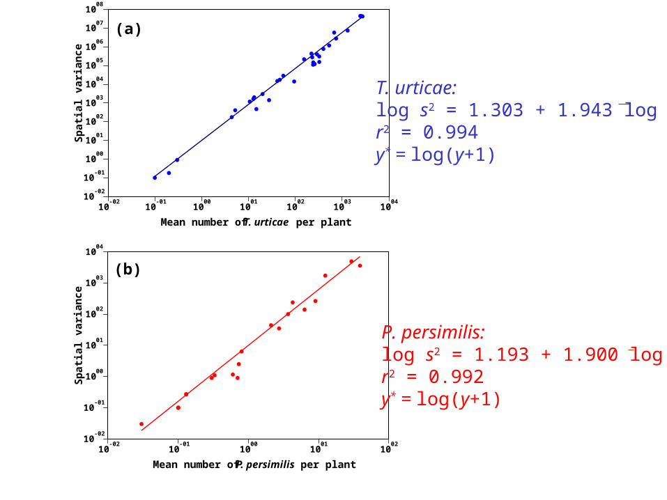
Mean number of T. urticae per plant
10-02
10-01
1000
1001
1002
1003
1004
1005
1006
1007
1008
Sp
ati
al
va
ria
nc
e
10-02
10-01
1000
1001
1002
Mean number of P. persimilis per plant
10-02
10-01
1000
1001
1002
1003
1004
Sp
ati
al
va
ria
nc
e
(b)
(a)
T. urticae:log s2 = 1.303 + 1.943 log xr2 = 0.994y* = log(y+1)
P. persimilis:log s2 = 1.193 + 1.900 log xr2 = 0.992y* = log(y+1)
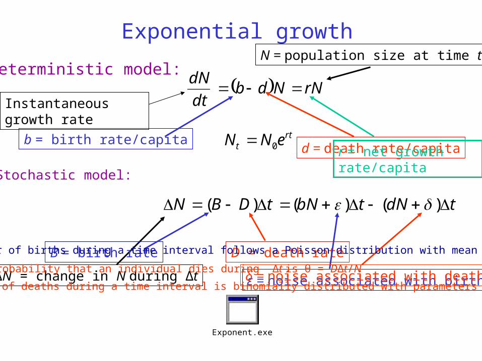
Exponential growth
Exponent.exe
Deterministic model: rNNdb
dt
dN
rtt eNN 0
Stochastic model:
tdNtbNtDBN )()()(
b = birth rate/capitad = death rate/capita
Instantaneous growth rate
N = population size at time t
r = net growth rate/capita
ΔN = change in N during Δt
B = birth rate D = death rate
ε = noise associated with birthsδ = noise associated with deaths
The number of births during a time interval follows a Poisson distribution with mean BΔt
The number of deaths during a time interval is binomially distributed with parameters (θ, N)
The probability that an individual dies during Δt is θ = DΔt/N
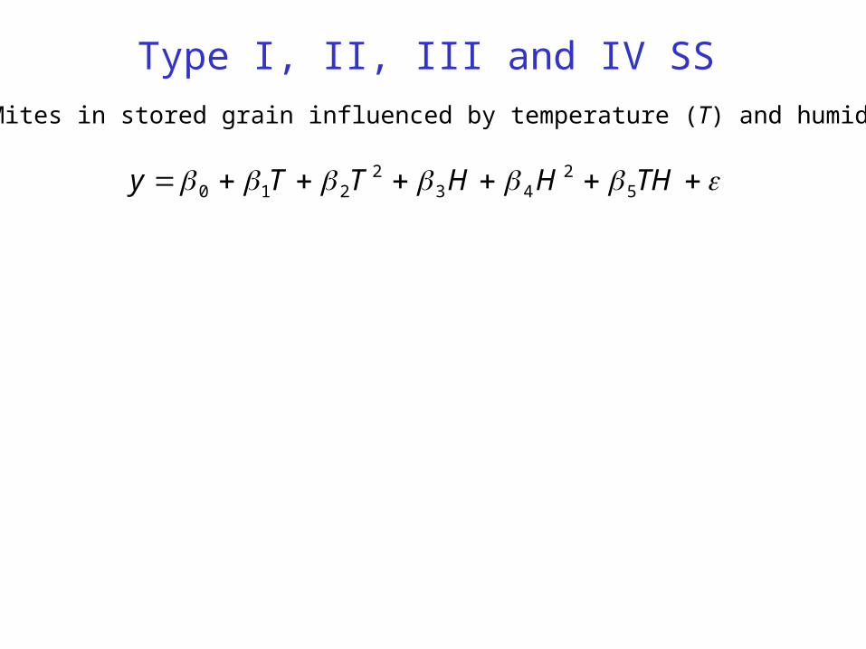
Type I, II, III and IV SS
Example: Mites in stored grain influenced by temperature (T) and humidity (H)
THHHTTy 52
432
210
DATA mites;
INFILE'h:\lin-mod\besvar\opg1-1.prn' FIRSTOBS=2;
INPUT pos $ depth T H Mites;
/* pos = position in store */
/* depth = depth in m */
/* T = Temperature of grain */
/* H = Humidity of grain */
/* Mites = number of mites in sampling unit */
logMites = log10(Mites+1); /* log transformation of Mites */
T2 = T**2; /* square temperature */
H2 = H**2; /* square humidity */
TH = T*H; /* product of temperature and humidity */
PROC GLM;
CLASS pos;
MODEL logMites = T T2 H H2 TH /SOLUTION SS1 SS3;
RUN;
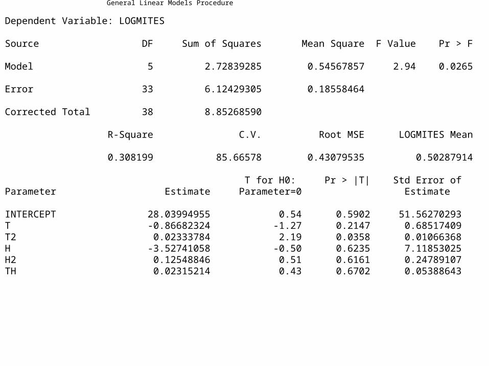
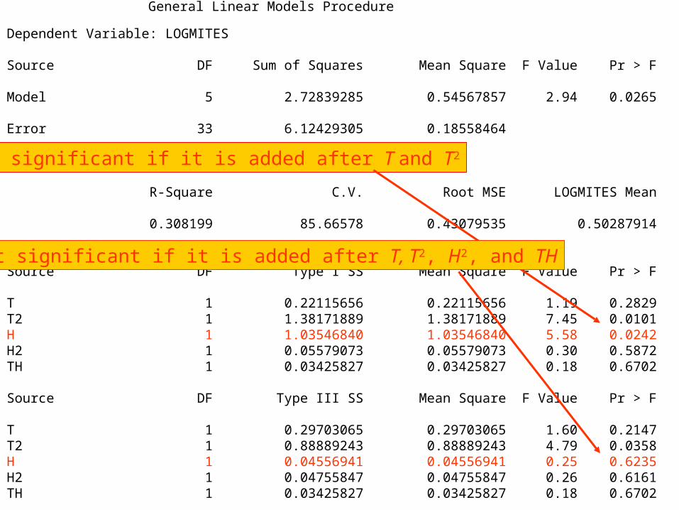
General Linear Models Procedure
Dependent Variable: LOGMITES Source DF Sum of Squares Mean Square F Value Pr > F Model 5 2.72839285 0.54567857 2.94 0.0265 Error 33 6.12429305 0.18558464 Corrected Total 38 8.85268590 R-Square C.V. Root MSE LOGMITES Mean 0.308199 85.66578 0.43079535 0.50287914 T for H0: Pr > |T| Std Error ofParameter Estimate Parameter=0 Estimate INTERCEPT 28.03994955 0.54 0.5902 51.56270293T -0.86682324 -1.27 0.2147 0.68517409T2 0.02333784 2.19 0.0358 0.01066368H -3.52741058 -0.50 0.6235 7.11853025H2 0.12548846 0.51 0.6161 0.24789107TH 0.02315214 0.43 0.6702 0.05388643
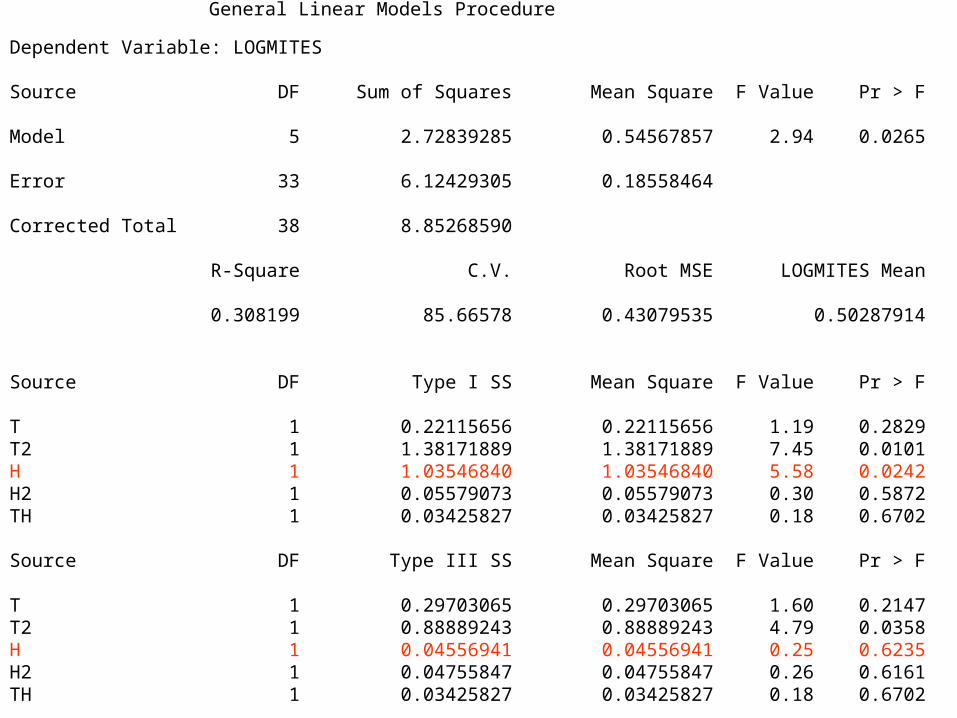
General Linear Models Procedure
Dependent Variable: LOGMITES Source DF Sum of Squares Mean Square F Value Pr > F Model 5 2.72839285 0.54567857 2.94 0.0265 Error 33 6.12429305 0.18558464 Corrected Total 38 8.85268590 R-Square C.V. Root MSE LOGMITES Mean 0.308199 85.66578 0.43079535 0.50287914 Source DF Type I SS Mean Square F Value Pr > F T 1 0.22115656 0.22115656 1.19 0.2829T2 1 1.38171889 1.38171889 7.45 0.0101H 1 1.03546840 1.03546840 5.58 0.0242H2 1 0.05579073 0.05579073 0.30 0.5872TH 1 0.03425827 0.03425827 0.18 0.6702 Source DF Type III SS Mean Square F Value Pr > F T 1 0.29703065 0.29703065 1.60 0.2147T2 1 0.88889243 0.88889243 4.79 0.0358H 1 0.04556941 0.04556941 0.25 0.6235H2 1 0.04755847 0.04755847 0.26 0.6161TH 1 0.03425827 0.03425827 0.18 0.6702
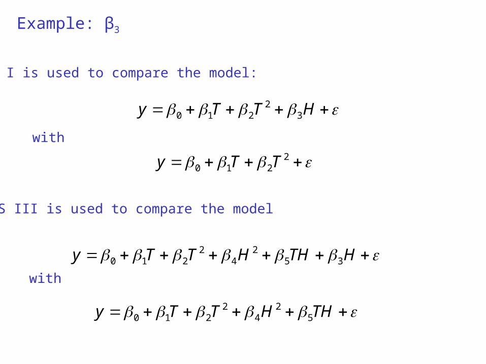
Example: β3
SS I is used to compare the model:
HTTy 32
210
with
2210 TTy
SS III is used to compare the model
HTHHTTy 352
42
210
with
THHTTy 52
42
210
General Linear Models Procedure
Dependent Variable: LOGMITES Source DF Sum of Squares Mean Square F Value Pr > F Model 5 2.72839285 0.54567857 2.94 0.0265 Error 33 6.12429305 0.18558464 Corrected Total 38 8.85268590 R-Square C.V. Root MSE LOGMITES Mean 0.308199 85.66578 0.43079535 0.50287914 Source DF Type I SS Mean Square F Value Pr > F T 1 0.22115656 0.22115656 1.19 0.2829T2 1 1.38171889 1.38171889 7.45 0.0101H 1 1.03546840 1.03546840 5.58 0.0242H2 1 0.05579073 0.05579073 0.30 0.5872TH 1 0.03425827 0.03425827 0.18 0.6702 Source DF Type III SS Mean Square F Value Pr > F T 1 0.29703065 0.29703065 1.60 0.2147T2 1 0.88889243 0.88889243 4.79 0.0358H 1 0.04556941 0.04556941 0.25 0.6235H2 1 0.04755847 0.04755847 0.26 0.6161TH 1 0.03425827 0.03425827 0.18 0.6702
H is significant if it is added after T and T2
H is not significant if it is added after T, T2, H2, and TH

How do we choose the best model?
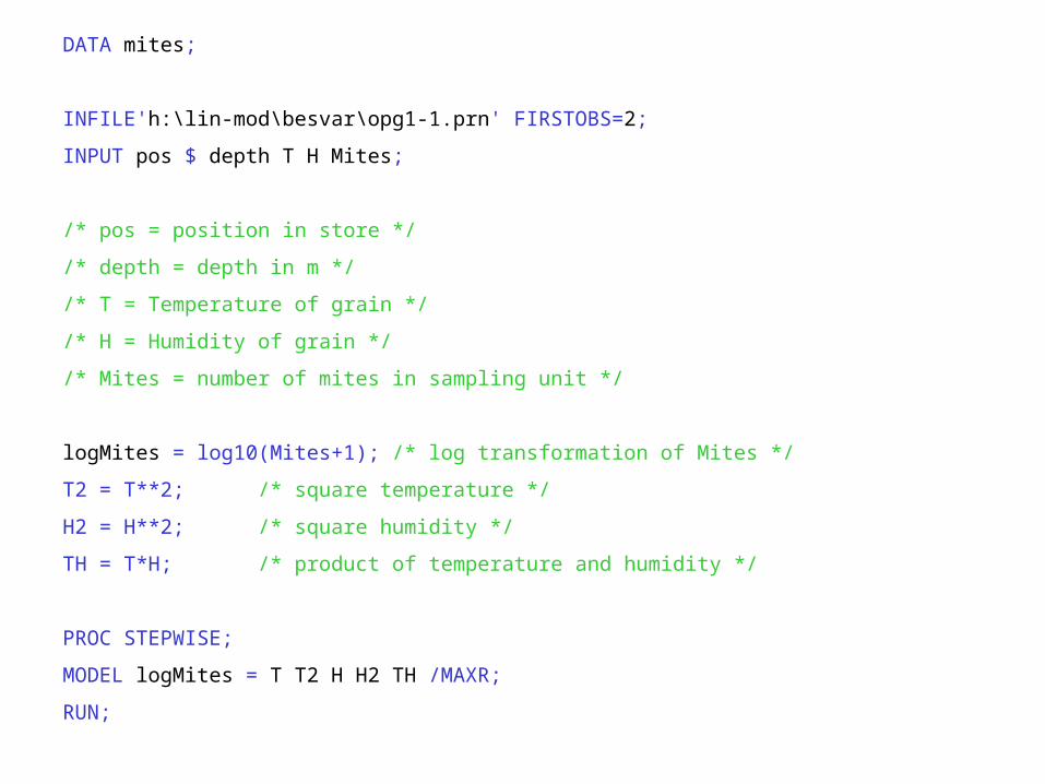
DATA mites;
INFILE'h:\lin-mod\besvar\opg1-1.prn' FIRSTOBS=2;
INPUT pos $ depth T H Mites;
/* pos = position in store */
/* depth = depth in m */
/* T = Temperature of grain */
/* H = Humidity of grain */
/* Mites = number of mites in sampling unit */
logMites = log10(Mites+1); /* log transformation of Mites */
T2 = T**2; /* square temperature */
H2 = H**2; /* square humidity */
TH = T*H; /* product of temperature and humidity */
PROC STEPWISE;
MODEL logMites = T T2 H H2 TH /MAXR;
RUN;
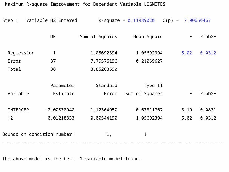
Maximum R-square Improvement for Dependent Variable LOGMITES
Step 1 Variable H2 Entered R-square = 0.11939020 C(p) = 7.00650467
DF Sum of Squares Mean Square F Prob>F
Regression 1 1.05692394 1.05692394 5.02 0.0312
Error 37 7.79576196 0.21069627
Total 38 8.85268590
Parameter Standard Type II
Variable Estimate Error Sum of Squares F Prob>F
INTERCEP -2.00838948 1.12364950 0.67311767 3.19 0.0821
H2 0.01218833 0.00544190 1.05692394 5.02 0.0312
Bounds on condition number: 1, 1
-----------------------------------------------------------------------------------
The above model is the best 1-variable model found.
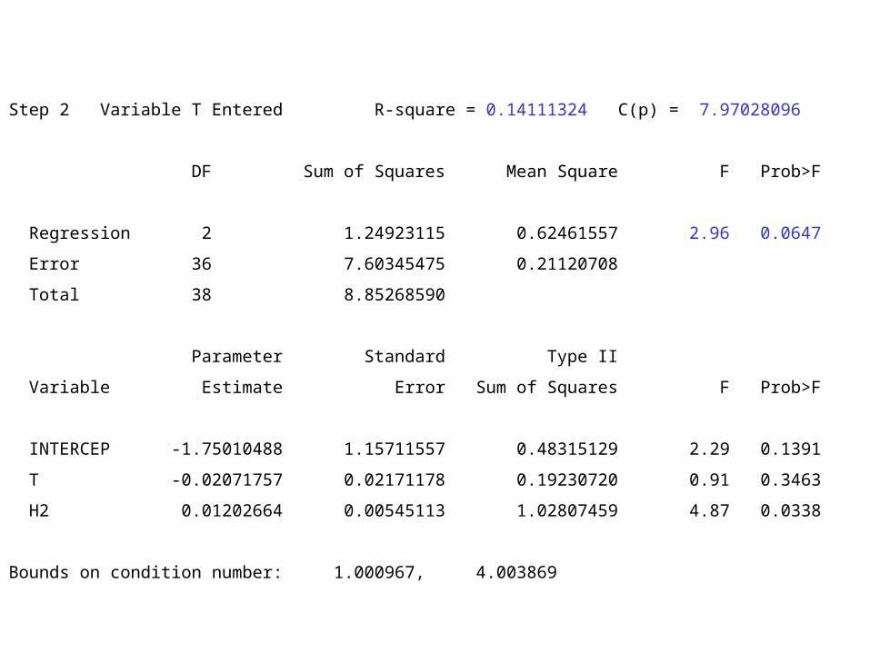
Step 2 Variable T Entered R-square = 0.14111324 C(p) = 7.97028096
DF Sum of Squares Mean Square F Prob>F
Regression 2 1.24923115 0.62461557 2.96 0.0647
Error 36 7.60345475 0.21120708
Total 38 8.85268590
Parameter Standard Type II
Variable Estimate Error Sum of Squares F Prob>F
INTERCEP -1.75010488 1.15711557 0.48315129 2.29 0.1391
T -0.02071757 0.02171178 0.19230720 0.91 0.3463
H2 0.01202664 0.00545113 1.02807459 4.87 0.0338
Bounds on condition number: 1.000967, 4.003869
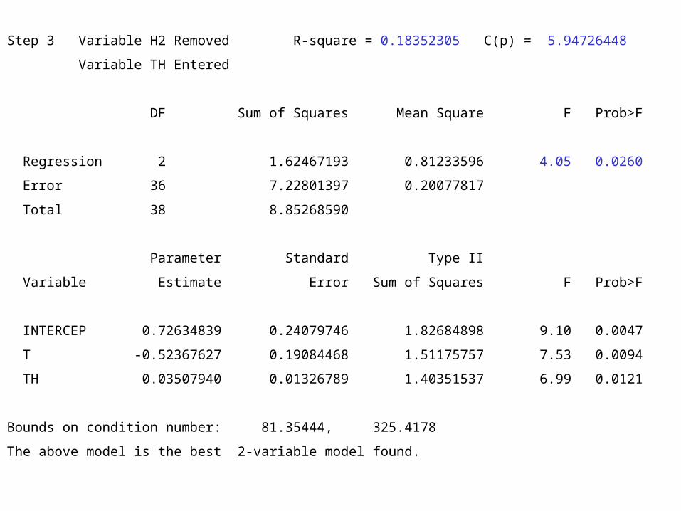
Step 3 Variable H2 Removed R-square = 0.18352305 C(p) = 5.94726448
Variable TH Entered
DF Sum of Squares Mean Square F Prob>F
Regression 2 1.62467193 0.81233596 4.05 0.0260
Error 36 7.22801397 0.20077817
Total 38 8.85268590
Parameter Standard Type II
Variable Estimate Error Sum of Squares F Prob>F
INTERCEP 0.72634839 0.24079746 1.82684898 9.10 0.0047
T -0.52367627 0.19084468 1.51175757 7.53 0.0094
TH 0.03507940 0.01326789 1.40351537 6.99 0.0121
Bounds on condition number: 81.35444, 325.4178
The above model is the best 2-variable model found.
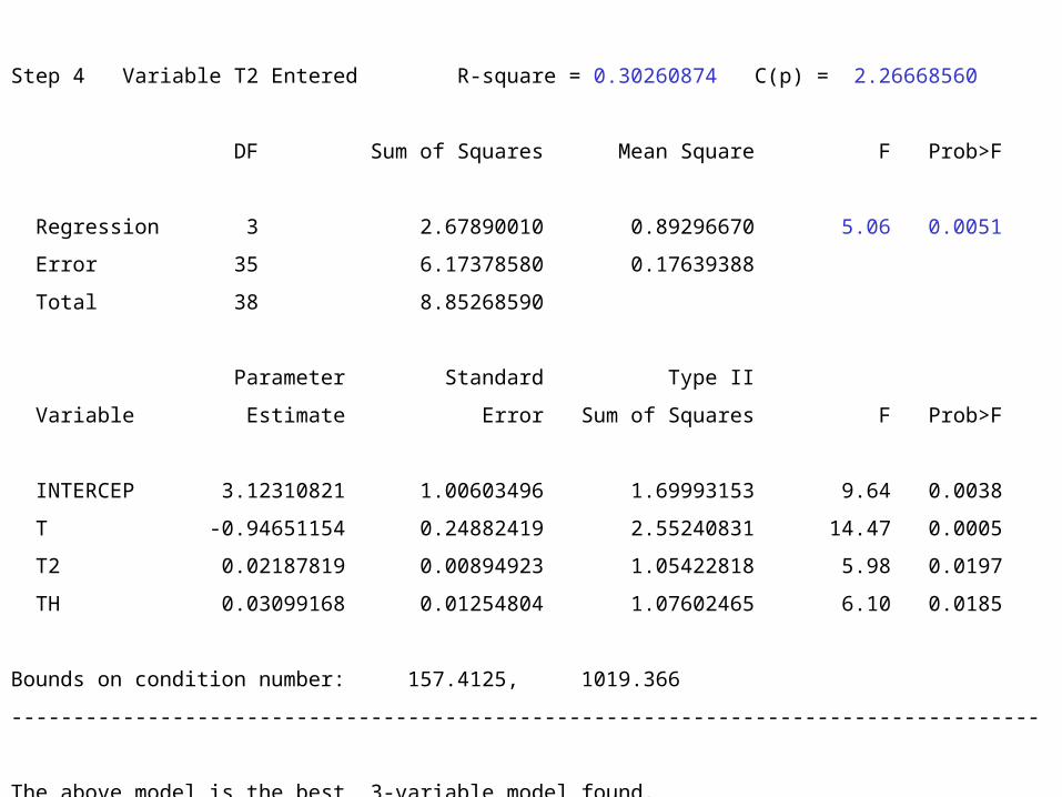
Step 4 Variable T2 Entered R-square = 0.30260874 C(p) = 2.26668560
DF Sum of Squares Mean Square F Prob>F
Regression 3 2.67890010 0.89296670 5.06 0.0051
Error 35 6.17378580 0.17639388
Total 38 8.85268590
Parameter Standard Type II
Variable Estimate Error Sum of Squares F Prob>F
INTERCEP 3.12310821 1.00603496 1.69993153 9.64 0.0038
T -0.94651154 0.24882419 2.55240831 14.47 0.0005
T2 0.02187819 0.00894923 1.05422818 5.98 0.0197
TH 0.03099168 0.01254804 1.07602465 6.10 0.0185
Bounds on condition number: 157.4125, 1019.366
-----------------------------------------------------------------------------------
The above model is the best 3-variable model found.
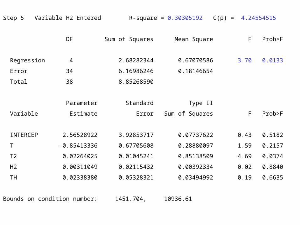
Step 5 Variable H2 Entered R-square = 0.30305192 C(p) = 4.24554515
DF Sum of Squares Mean Square F Prob>F
Regression 4 2.68282344 0.67070586 3.70 0.0133
Error 34 6.16986246 0.18146654
Total 38 8.85268590
Parameter Standard Type II
Variable Estimate Error Sum of Squares F Prob>F
INTERCEP 2.56528922 3.92853717 0.07737622 0.43 0.5182
T -0.85413336 0.67705608 0.28880097 1.59 0.2157
T2 0.02264025 0.01045241 0.85138509 4.69 0.0374
H2 0.00311049 0.02115432 0.00392334 0.02 0.8840
TH 0.02338380 0.05328321 0.03494992 0.19 0.6635
Bounds on condition number: 1451.704, 10936.61
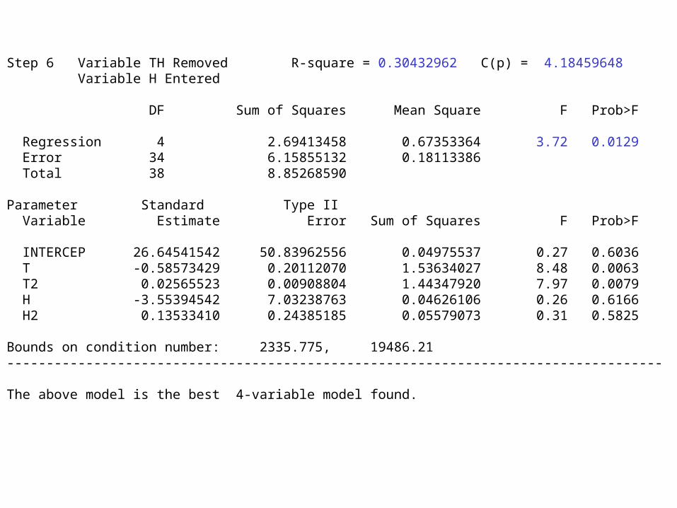
Step 6 Variable TH Removed R-square = 0.30432962 C(p) = 4.18459648 Variable H Entered DF Sum of Squares Mean Square F Prob>F Regression 4 2.69413458 0.67353364 3.72 0.0129 Error 34 6.15855132 0.18113386 Total 38 8.85268590
Parameter Standard Type II Variable Estimate Error Sum of Squares F Prob>F INTERCEP 26.64541542 50.83962556 0.04975537 0.27 0.6036 T -0.58573429 0.20112070 1.53634027 8.48 0.0063 T2 0.02565523 0.00908804 1.44347920 7.97 0.0079 H -3.55394542 7.03238763 0.04626106 0.26 0.6166 H2 0.13533410 0.24385185 0.05579073 0.31 0.5825 Bounds on condition number: 2335.775, 19486.21----------------------------------------------------------------------------------- The above model is the best 4-variable model found.
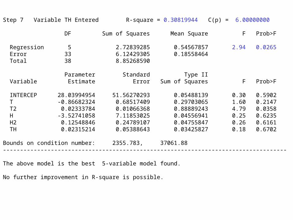
Step 7 Variable TH Entered R-square = 0.30819944 C(p) = 6.00000000 DF Sum of Squares Mean Square F Prob>F Regression 5 2.72839285 0.54567857 2.94 0.0265 Error 33 6.12429305 0.18558464 Total 38 8.85268590 Parameter Standard Type II Variable Estimate Error Sum of Squares F Prob>F INTERCEP 28.03994954 51.56270293 0.05488139 0.30 0.5902 T -0.86682324 0.68517409 0.29703065 1.60 0.2147 T2 0.02333784 0.01066368 0.88889243 4.79 0.0358 H -3.52741058 7.11853025 0.04556941 0.25 0.6235 H2 0.12548846 0.24789107 0.04755847 0.26 0.6161 TH 0.02315214 0.05388643 0.03425827 0.18 0.6702 Bounds on condition number: 2355.783, 37061.88----------------------------------------------------------------------------------- The above model is the best 5-variable model found. No further improvement in R-square is possible.
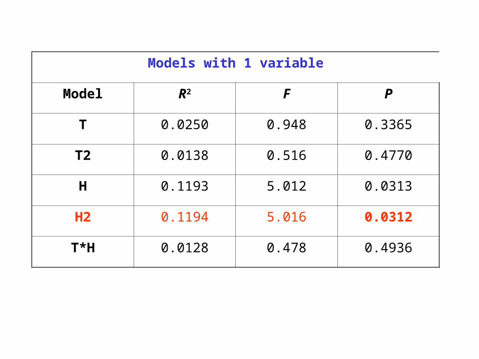
Models with 1 variable
Model R2 F P
T 0.0250 0.948 0.3365
T2 0.0138 0.516 0.4770
H 0.1193 5.012 0.0313
H2 0.1194 5.016 0.0312
T*H 0.0128 0.478 0.4936
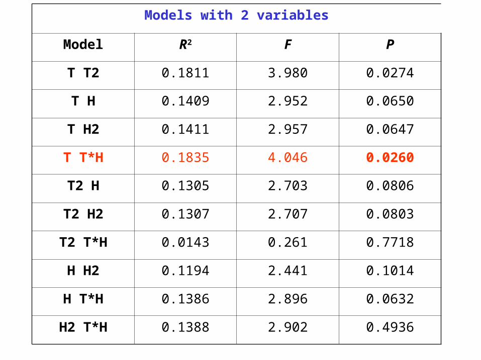
Models with 2 variables
Model R2 F P
T T2 0.1811 3.980 0.0274
T H 0.1409 2.952 0.0650
T H2 0.1411 2.957 0.0647
T T*H 0.1835 4.046 0.0260
T2 H 0.1305 2.703 0.0806
T2 H2 0.1307 2.707 0.0803
T2 T*H 0.0143 0.261 0.7718
H H2 0.1194 2.441 0.1014
H T*H 0.1386 2.896 0.0632
H2 T*H 0.1388 2.902 0.4936
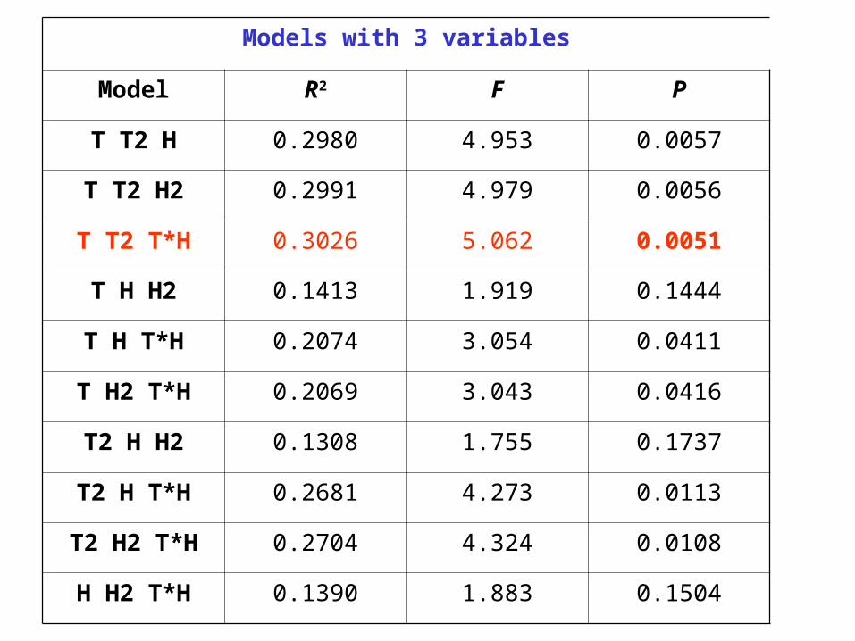
Models with 3 variables
Model R2 F P
T T2 H 0.2980 4.953 0.0057
T T2 H2 0.2991 4.979 0.0056
T T2 T*H 0.3026 5.062 0.0051
T H H2 0.1413 1.919 0.1444
T H T*H 0.2074 3.054 0.0411
T H2 T*H 0.2069 3.043 0.0416
T2 H H2 0.1308 1.755 0.1737
T2 H T*H 0.2681 4.273 0.0113
T2 H2 T*H 0.2704 4.324 0.0108
H H2 T*H 0.1390 1.883 0.1504
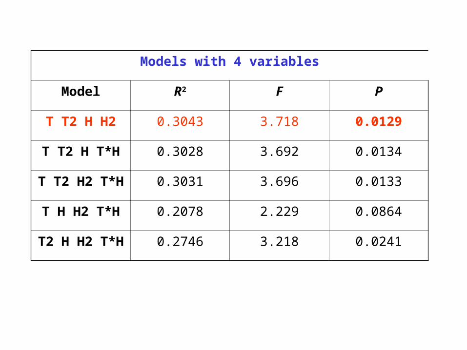
Models with 4 variables
Model R2 F P
T T2 H H2 0.3043 3.718 0.0129
T T2 H T*H 0.3028 3.692 0.0134
T T2 H2 T*H 0.3031 3.696 0.0133
T H H2 T*H 0.2078 2.229 0.0864
T2 H H2 T*H 0.2746 3.218 0.0241
Models with 5 variables
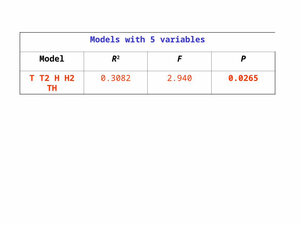
Model R2 F P
T T2 H H2 TH 0.3082 2.940 0.0265
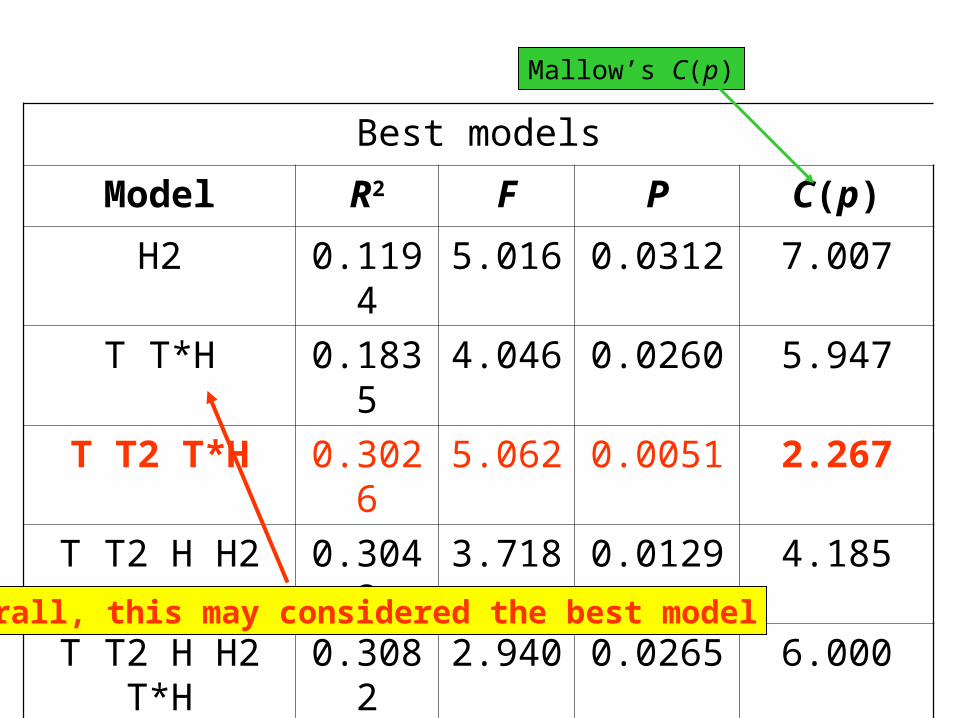
Best models
Model R2 F P C(p)
H2 0.1194 5.016 0.0312 7.007
T T*H 0.1835 4.046 0.0260 5.947
T T2 T*H 0.3026 5.062 0.0051 2.267
T T2 H H2 0.3043 3.718 0.0129 4.185
T T2 H H2 T*H 0.3082 2.940 0.0265 6.000
Overall, this may considered the best model
Mallow’s C(p)
Model control
DATA mites;
INFILE'h:\lin-mod\besvar\opg1-1.prn' FIRSTOBS=2;
INPUT pos $ depth T H Mites;
LogMites = log10(Mites+1); /* transform dependent variable */
T2 = T**2; /* square temperature */
H2 = H**2; /* square humidity */
TH = T*H; /* interaction between temperature and humidity */
PROC REG; /* Multiple regression analysis */
MODEL logMites = T T2 H H2 TH;
OUTPUT out = new P = pred R = res;
RUN;
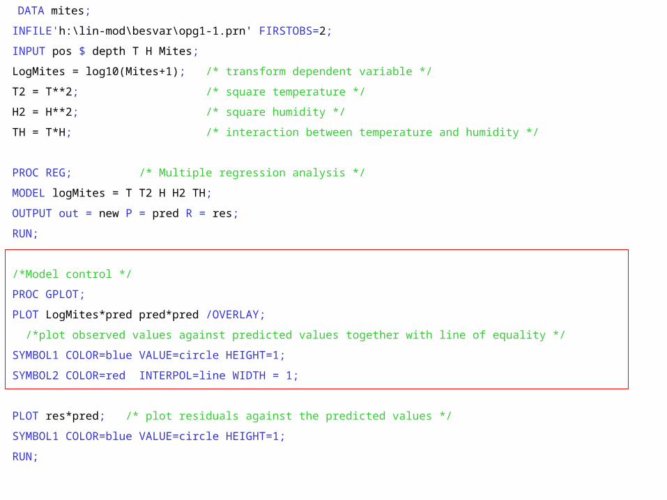
/*Model control */
PROC GPLOT;
PLOT LogMites*pred pred*pred /OVERLAY;
/*plot observed values against predicted values together with line of equality */
SYMBOL1 COLOR=blue VALUE=circle HEIGHT=1;
SYMBOL2 COLOR=red INTERPOL=line WIDTH = 1;
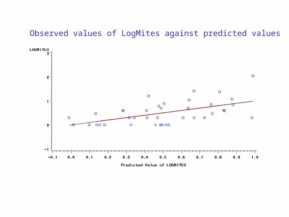
PLOT res*pred; /* plot residuals against the predicted values */
SYMBOL1 COLOR=blue VALUE=circle HEIGHT=1;
RUN;
Observed values of LogMites against predicted values
DATA mites;
INFILE'h:\lin-mod\besvar\opg1-1.prn' FIRSTOBS=2;
INPUT pos $ depth T H Mites;
LogMites = log10(Mites+1); /* transform dependent variable */
T2 = T**2; /* square temperature */
H2 = H**2; /* square humidity */
TH = T*H; /* interaction between temperature and humidity */
PROC REG; /* Multiple regression analysis */
MODEL logMites = T T2 H H2 TH;
OUTPUT out = new P = pred R = res;
RUN;
/*Model control */
PROC GPLOT;
PLOT LogMites*pred pred*pred /OVERLAY;
/*plot observed values against predicted values together with line of equality */
SYMBOL1 COLOR=blue VALUE=circle HEIGHT=1;
SYMBOL2 COLOR=red INTERPOL=line WIDTH = 1;
PLOT res*pred; /* plot residuals against the predicted values */
SYMBOL1 COLOR=blue VALUE=circle HEIGHT=1;
RUN;
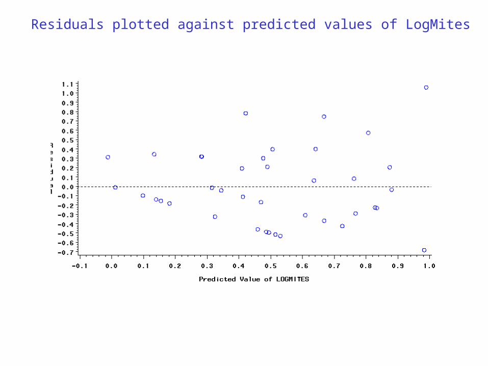
Residuals plotted against predicted values of LogMites
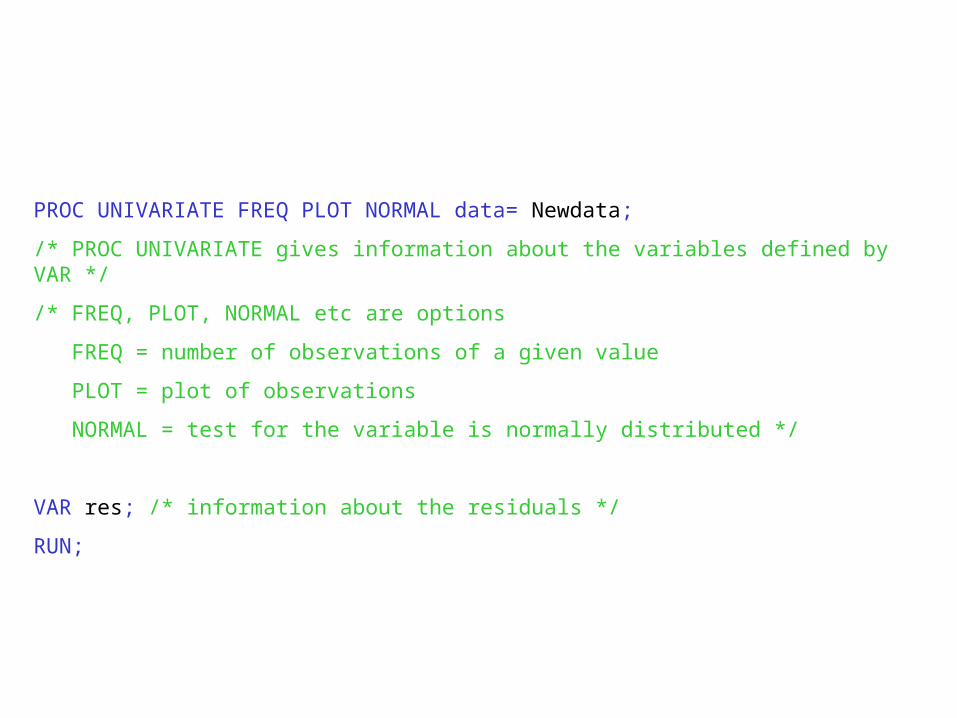
PROC UNIVARIATE FREQ PLOT NORMAL data= Newdata;
/* PROC UNIVARIATE gives information about the variables defined by VAR */
/* FREQ, PLOT, NORMAL etc are options
FREQ = number of observations of a given value
PLOT = plot of observations
NORMAL = test for the variable is normally distributed */
VAR res; /* information about the residuals */
RUN;
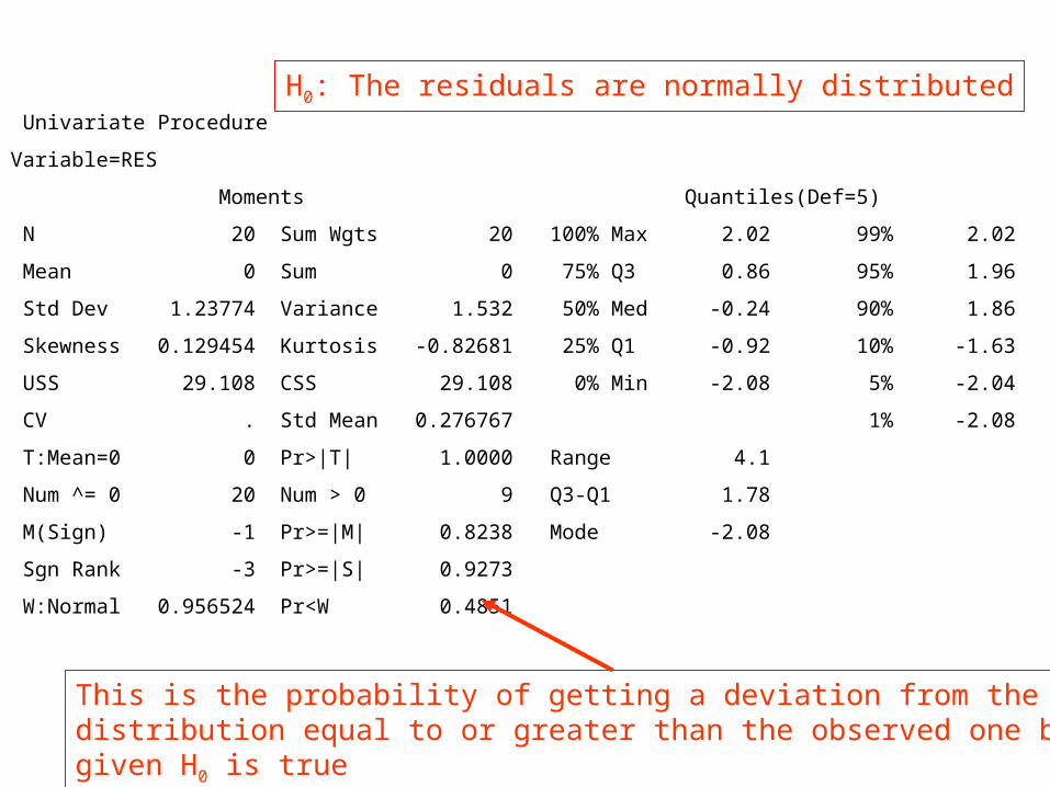
Univariate Procedure
Variable=RES
Moments Quantiles(Def=5)
N 20 Sum Wgts 20 100% Max 2.02 99% 2.02
Mean 0 Sum 0 75% Q3 0.86 95% 1.96
Std Dev 1.23774 Variance 1.532 50% Med -0.24 90% 1.86
Skewness 0.129454 Kurtosis -0.82681 25% Q1 -0.92 10% -1.63
USS 29.108 CSS 29.108 0% Min -2.08 5% -2.04
CV . Std Mean 0.276767 1% -2.08
T:Mean=0 0 Pr>|T| 1.0000 Range 4.1
Num ^= 0 20 Num > 0 9 Q3-Q1 1.78
M(Sign) -1 Pr>=|M| 0.8238 Mode -2.08
Sgn Rank -3 Pr>=|S| 0.9273
W:Normal 0.956524 Pr<W 0.4851
H0: The residuals are normally distributed
This is the probability of getting a deviation from the normaldistribution equal to or greater than the observed one by chancegiven H0 is true
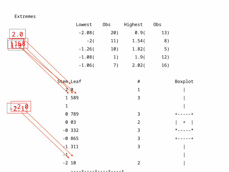
Extremes
Lowest Obs Highest Obs
-2.08( 20) 0.9( 13)
-2( 11) 1.54( 8)
-1.26( 10) 1.82( 5)
-1.08( 1) 1.9( 12)
-1.06( 7) 2.02( 16)
Stem Leaf # Boxplot
2 0 1 |
1 589 3 |
1 |
0 789 3 +-----+
0 03 2 | + |
-0 332 3 *-----*
-0 865 3 +-----+
-1 311 3 |
-1 |
-2 10 2 |
----+----+----+----+
2.0
1.51.81.9
-2.0-2.1
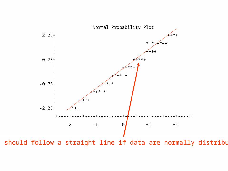
Normal Probability Plot
2.25+ ++*+
| * * +*++
| ++++
0.75+ *+**+
| ++**+
| +*** *
-0.75+ ++*+*
| +*+* *
| ++*+
-2.25+ +*++
+----+----+----+----+----+----+----+----+----+----+
-2 -1 0 +1 +2
Points should follow a straight line if data are normally distributed
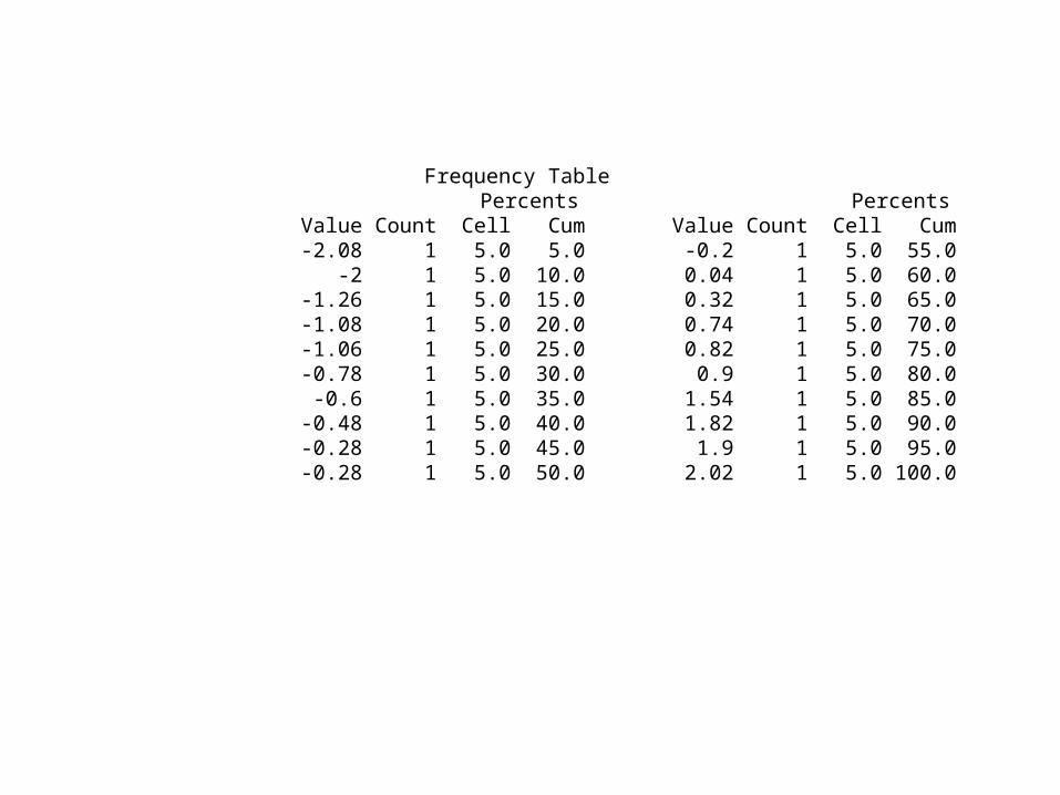
Frequency Table Percents Percents Value Count Cell Cum Value Count Cell Cum -2.08 1 5.0 5.0 -0.2 1 5.0 55.0 -2 1 5.0 10.0 0.04 1 5.0 60.0 -1.26 1 5.0 15.0 0.32 1 5.0 65.0 -1.08 1 5.0 20.0 0.74 1 5.0 70.0 -1.06 1 5.0 25.0 0.82 1 5.0 75.0 -0.78 1 5.0 30.0 0.9 1 5.0 80.0 -0.6 1 5.0 35.0 1.54 1 5.0 85.0 -0.48 1 5.0 40.0 1.82 1 5.0 90.0 -0.28 1 5.0 45.0 1.9 1 5.0 95.0 -0.28 1 5.0 50.0 2.02 1 5.0 100.0