Embed Size (px)
Citation preview
Research ArticleExperimental Characterization of LTE Wireless Links inHigh-Speed Trains
Tomaacutes Domiacutenguez-Bolantildeo Joseacute Rodriacuteguez-Pintildeeiro Joseacute A Garciacutea-Naya and Luis Castedo
Universidade da Coruna A Coruna Spain
Correspondence should be addressed to Tomas Domınguez-Bolano tomasbolanoudces
Received 25 May 2017 Accepted 3 August 2017 Published 28 September 2017
Academic Editor Yin Xuefeng
Copyright copy 2017 Tomas Domınguez-Bolano et al This is an open access article distributed under the Creative CommonsAttribution License which permits unrestricted use distribution and reproduction in any medium provided the original work isproperly cited
Multimedia and data-based services experienced a nonstopping growth over the last few years People are continuously on themove using devices to access multimedia contents or other data-based services Due to this railway companies are showing a greatinterest in deploying broadband mobile wireless networks in high-speed-trains with the aim of supporting both passenger servicesprovisioning as well as automatic train control and signaling Nowadays the most widely used technology for communicationsbetween trains and the railway infrastructure is GSM for Railways (GSM-R) however it has limited capabilities to support suchadvanced services Due to its success in the mass market Long Term Evolution (LTE) seems to be the best candidate to substituteGSM-R In this paper we experimentally characterize the downlink between an LTE Evolved NodeB (eNodeB) and a high-speedtrain in a commercial high-speed line We consider two links the one between the eNodeB and the antennas placed outdoors onthe train roof and the direct link between the eNodeB and a receiver inside the train Such a characterization consists in assessingthe path loss the Signal to Noise Ratio the 119870-Factor the Power Delay Profile the delay spread and the Doppler Power SpectralDensity
1 Introduction
Railway communications can be divided into two groups(a) train control signaling and safety-related communicationsand (b) noncritical communications both for train staff andpassengers While the first kind of communications usuallydoes not require high data rates it in turn imposes stringentconstraints to the Quality of Service (QoS) [1ndash5] Operationaland functional requirements for the railway environmentrequire in fact reduced delays or call setup times as wellas very reduced service interruptions The second type ofrailway communications demands higher throughputs (egaccess to multimedia services) but they do not impose sostrict requirements in terms of reliability
Nowadays the most widely used technology for traincontrol signaling and safety-related communicationsbetween trains is based on GSM for Railways (GSM-R) andrequires a specific network deployment with base stationslocated along the track The GSM-R which is based on themature Global System for Mobile Communications (GSM)
technology provides a continuous communication channelbetween the train driver and the ground controllers beingwell-suited to perform emergency calls selective phone callsor small data transmission However GSM-R has reducedcapabilities to support more advanced services such asautomatic pilot or provisioning broadband communicationsto train staff
Besides that multimedia and data-based services expe-rienced a nonstopping growth over the last few years [1]People are continuously on the move using devices to accessmultimedia contents or other data-based services Whereassometimes the transmission of a few data bits is enoughcontinuous streaming of multimedia data is required in othersituations In most cases users are connected to general-purpose mobile networks However railway companies areaware of the market opportunity and aim to provide pas-sengers with multimedia services andor broadband Internetaccess onboard The Mobile-Relay technique has been pro-posed in [6] as a way to provide coverage to passengers basedon a relaying scheme (a link from the cellular base station to
HindawiWireless Communications and Mobile ComputingVolume 2017 Article ID 5079130 20 pageshttpsdoiorg10115520175079130
2 Wireless Communications and Mobile Computing
an external antenna installed on the train which is relayed toa local base station inside the train carriage)
Taking into account the big success of Long TermEvolution (LTE) in the evolution of mobile networks itseems reasonable to consider LTE as the best candidateto substitute GSM-R as the fundamental technology forrailway communications as well as provisioning services topassengers While in previous publications we studied thesuitability of LTE to fulfill the operational and functionalrequirements for the railway environment (eg see [1ndash4]) inthis paper we account for the detailed characterization of thewireless link based on LTE measurements in a high-speedtrain line in Spain We consider both the channel betweenan Evolved NodeB (eNodeB) and a passenger inside a high-speed train as well as the direct channel between the eNodeBand the outdoor antennas installed on the train carriage
The first step for migrating GSM-R into LTE is to assessthe performance of such a communications system for therailway environment Knowledge of the wireless channelcharacteristics is the fundamental basis for the planningof wireless communication networks and the design oftransceivers [1 7] However HST communications demandfor the evaluation of specific scenarios which are typical inmost railway lines such as [1] rural macrocell hilly terrainviaducts cuttings or tunnels Hence in recent years a lotof attention has been put to measurement-based analysis tocharacterize the different types of high-speed railway scenar-ios In [8ndash11] several parameters of the channel were analyzedand modeled for a viaduct scenario based on measurementscarried out using GSM-R Base Stations (BSs) at 930MHz In[12] the channel is characterized and modeled for a cuttingscenario based on measurements carried out using GSM-RBSs at 930MHzThe papers [13ndash15] analyze the channel for aviaduct scenario considering a carrier frequency of 235GHzIn [16] a hilly terrain scenario is considered and the delayandDoppler spread is characterized for a carrier frequency of24GHz In [17] the authors use the commercially deployedLTE base stations along the HST railway between Beijing andShanghai (with a total distance of 1318 km) to characterizestatistically the parameters of the observed channels
In our case we did not perform the measurements byemploying a general-purpose mobile network deploymentduring the train operation However different from otherworks we installed an eNodeB taking advantage of theavailable infrastructure for GSM-R in the considered high-speed train lineWe considered a carrier frequency of 26GHzand the 10MHz profile of LTE Furthermore we deployedtwo sectors and the corresponding eNodeB antenna panelswere placed in the same tower where the GSM-R antennasare installed Since we measured LTE standard-compliantsignals tasks like time and frequency synchronization orchannel estimation were performed considering exclusivelythe same information that a commercial receiver woulduse (ie synchronization signals and pilots) We could alsoperform different train passes along a segment of about7 km long centered at the eNodeB site with distinct trainspeeds and varying the data traffic At the receiver (train)side we could access the external antennas of the trainbeing able to evaluate the eNodeB-train wireless link in a
realistic way We also considered antennas installed indoorsto model the direct eNodeB-passenger link Furthermorehigh-resolution results are obtained from our measurements(which are freely available for other research groups) sincewe continuously capture the signal at the receiver during thewhole measurement campaigns
The main contribution of this paper is the complete anddetailed characterization of the downlink between a com-mercial LTE eNodeB and a train moving at high velocitiesalong a track in commercial operation in a rural area inSpain We consider two links the one between the eNodeBand the antennas placed outdoors on the train roof andthe direct link between the eNodeB and a receiver insidethe train Such a characterization consists in assessing thepath loss the Signal to Noise Ratio (SNR) the 119870-Factorthe Power Delay Profile (PDP) the delay spread and theDoppler Power Spectral Density (PSD) for different trainspeeds Finally we showed the specific characteristics ofthe railway channel and the impact of the train speed onthem Besides that the mathematical description of all theprocedures followed to obtain the results is detailed Inparticular mathematical descriptions in both discrete timeand frequency are provided for all the estimated parameterschannel response synchronization SNR path loss119870-FactorPDP delay spread andDoppler PSD Additionally guidelinesabout the drawbacks and pitfalls to be considered for thedifferent analysis methods are provided
The structure of the paper is as follows Section 2describes in detail the environment as well as the experi-mental setup and procedure considered for the evaluationsSection 3 explains the basic aspects of the signal processingperformed at the receiver including the signal synchro-nization or the channel and SNR estimation Section 4characterizes the path loss for both the eNodeB-train anddirect eNodeB-passenger links while Section 5 studies theeNodeB-train channel condensed parameters such as the119870-Factor the PDP the delay spread and the Doppler PSD InSection 6 we study significant regions of the train path indetail showing how train infrastructure elements can impacton the wireless link Finally Section 7 concludes the paper
2 Experimental Setup
We evaluated experimentally the links between an eNodeBand receive antennas placed on the roof of a train carriage aswell as a mobile receiver inside the train By first evaluatingthe path loss we motivate the need of a relay architectureto distribute the signal inside the train through repeatersor Access Points (Aps) while employing external (train-mounted) antennas for the link between the train and theeNodeB Then the effects of the high-speed on the latter linkare studied in detail by means of parameters such as the 119870-Factor the PDP or the Doppler PSD taking into account theeffects at high speeds
Ameasurement campaignwas conducted in a high-speedtrain line in commercial operation Different from otherworks we could access the railway environment and equip-ment which enabled us to perform different experimentsduring maintenance periods (mainly overnight) by freely
Wireless Communications and Mobile Computing 3
eNB
0 200 300100Instantaneous speed (kmh)
100 200 3000Instantaneous speed (kmh)
eNB
102
101
100
99
98
97
96
95
94
93
Kilo
met
ric p
oint
(km
)
Top speed 100 EGB Top speed 200 EGB
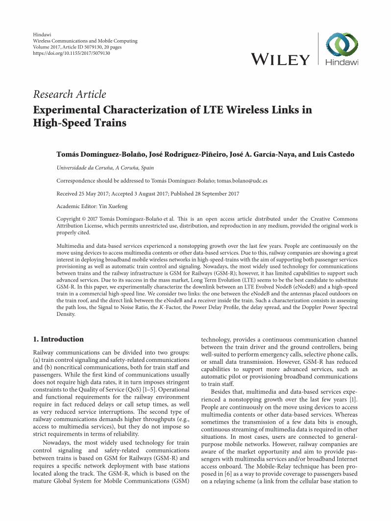
Figure 1 Map of the scenario considered for the measurementsThe instantaneous train speed is shown for each point of the trajectory bothfor the cases considering a maximum speed of 100 kmh and 200 kmh The position of the eNodeB is also specified Map Image by copy2017DigitalGlobe Cartography Institute of Andalucıa Map Data by copy2017 Google National Geographic Institute of Spain
controlling the train movement as well as the transmittedsignals Even more one of the most important features ofour experiments is that instead of using eNodeB deployedfor general-purpose mobile cellular communications weinstalled an eNodeB in one of the GSM-R sites specifi-cally devoted for railway communications Furthermore weobtained the permission to employ the carrier frequencyat 26GHz which is commercially used in such an areaMeasurements were carried out along a track segment ofapproximately 7 km long centered at the GSM-R site in arural area The considered train was specifically designed totest all the systems each time a new line is opened hencethe access to some resources such as the external antennasinstalled on its roof was granted This allowed us to analyzethe use of LTE for high-speed train applications at the actualenvironment and employing the specific infrastructure of therailway operator It is also worth noting that the transmitpower was high enough so that the SNR level exceeds20 dB (when using antennas placed outdoors) This allowsfor correctly synchronizing most of the LTE frames withouterrors hence enabling us to analyze the signal along thewholetrain path that is instead of only sampling the acquiredsignal during short time intervals while the train movesalong the track our equipment acquires the transmitted LTEframes in a continuous fashion The following subsectionsdescribe the details of the measurement environment theequipment used and the methodology followed to performthe measurements
21 Measurement Environment
211 Test Track The considered high-speed train line con-nects Cordoba and Malaga (Spain) and is designed to cope
with speeds up to 330 kmh The measured segment islocated between the Kilometric Points (KPs) 930 and 1020whereas the GSM-R site is located at KP 97075 (the exactGlobal Positioning System (GPS) coordinates of the site are37∘4101584031410158401015840N 4∘431015840125210158401015840W) as imaged in Figure 1 TheAntequera-Santa Ana Railway Station (KP 96800) and aTraffic Management Center are also located in the vicinity ofthe GSM-R site
212 Test Train The considered test train was the so-calledSeneca laboratory train (Talgo A-330) provided by the Span-ish Railway Infrastructure Administrator (ADIF) imagedin Figure 2(a) The train was intended for infrastructureinspections and it was extensively used in testing activitiesfor the deployment of the European Rail TrafficManagementSystemEuropean Train Control System (ERTMSETCS)standard in Spanish high-speed lines Electrically poweredthe train can reach a maximum speed of 363 kmh althoughthe maximum considered speed for our measurements waslimited to 200 kmh because the time (and also the distance)required to reach a higher speed is extremely large thuslimiting the number of trials to be performed in a typicalmeasurement session during the night The train is 8092mlong and includes an inner panel (see Figure 2(b)) whichallows for the connection to the external antennas on itsroof (see Figure 2(c)) two of them are multiband antennas(800 900 1800 1900 UMTS UMTSII W-LAN and GPS)Kathrein 870 10003 whereas the other two are Kathrein870 10007 (without GPS) both featuring a 0 dB gain anda Voltage Standing Wave Ratio (VSWR) smaller than 20 1at the considered carrier frequency of 26GHz During themeasurements we used two external antennas one of eachtype The GPS connection is used by the GPS-disciplined
4 Wireless Communications and Mobile Computing
(a) Photography of the whole train (b) Inner panel for con-nection to the outdoor an-tennas
(c) Outdoor antennas onthe roof of the train car-riage (Kathrein 870 10003and 870 10007) The fourantennas are marked withred ellipses
Figure 2 Seneca laboratory train (Talgo A-330)
(a) Image of the tower andthe two cabins for telecom-munications equipment
(b) Antenna installed at the tower (forsouth sector)
Figure 3 Pictures of the GSM-R site
oscillators included in the measurement equipment and tomatch the acquired samples with the estimated position andvelocity of the train
22 Measurement Equipment
221 Ground Equipment The GSM-R site imaged in Fig-ure 3(a) includes a 40m height tower with antennas fordifferent wireless technologies and two cabins where thecommunications equipment is installed A commercial LTEeNodeB was set up inside one of the available cabins and tworemote radio headsweremounted at the tower structure eachone connected to two antenna elements of a different antennapanel (see Figure 3(b)) Such antenna panels (Moyano MY-DTBSBS17276518) were placed at a height of 20m and ori-entated as the available GSM-R antennas At the consideredcarrier frequency (26GHz) these cross-polarized antennas
Table 1 Ground antennas orientation in both vertical (with respectto the horizontal plane) and horizontal (with respect to the northdirection) dimensions
Sector Antenna orientation [∘]Azimuth Elevation
North 355 0South 175 minus14
feature a gain of 18 dBi and a half-power beam width of62∘ (horizontal) and 5∘ (vertical) as imaged in the radiationpattern shown in Figure 4 Each antenna panel is used todeploy a sector hence two sectors are used named as ldquonorthsectorrdquo and ldquosouth sectorrdquo respectively (see Figure 1) Table 1shows the orientation of the ground antennas
Wireless Communications and Mobile Computing 5
Horizontal beamVertical beam
0∘
300∘
330∘
270∘
240∘
210∘
180∘150∘
120∘
90∘
60∘
30∘
minus6 >
minus3 >
Figure 4 Radiation pattern for the transmit antennas (MoyanoMY-DTBSBS17276518) Both the vertical and horizontal radiationpatterns are shown
The eNodeB was configured to transmit an LTE signalwith the profile of 10MHz bandwidth transmit diversity (asingle transmit block is encoded and transmitted throughtwo different antennas Precoding is performed in orderto separate the two different antennas) and normal cyclicprefix (CP) length (the first Orthogonal Frequency-DivisionMultiplexing (OFDM) symbol of an LTE slot (a slot occupieshalf a subframe) has a cyclic prefix length of 119873CP
long = 80samples (52083 microseconds) whereas for the remainingsix OFDM symbols the cyclic prefix is reduced to 119873CP
short =72 samples (46875 microseconds)) More details regardingthe transmit signal configuration are specified in Table 2Note that two configurations for data traffic transmissionwere considered (a commercial LTE receiver (different thanthose employed to produce the results shown in the paper)is connected as the only user to the eNodeB this way we cancapture the signals between the eNodeB and the commercialreceiver to be used for our evaluations)
(i) Maximum throughput all the resource blocks of theLTE signal are filled in with data Hence the max-imum payload of LTE is used for the configurationparameters specified in Table 2
(ii) ETCS + VoIP a stream of European Train ControlSystem (ETCS) data traffic is transmitted in parallelwith a Voice over Internet Protocol (VoIP) call
In both cases the receiver used in the measurements has noa priori knowledge about the transmit data
222 Onboard Equipment The onboard equipment consistsof two nodes from the so-called GTEC Testbed (described
Table 2 LTE testbed configuration parameters
Parameter ValueSampling frequency 119891119904 1536MHzTransmit power 46 dBmMaximum antenna gain 18 dBi (TX) 0 dBi (RX)Carrier frequency 26GHzBandwidth 10MHz (9MHz occupied)
Transmission scheme Transmission mode 2 (transmitdiversity) [18]
Cyclic prefix length Normal
in [19 20]) operating in receive-only mode Each of themincludes an EttusNational Instruments Universal SoftwareRadio Peripheral (USRP) B210 (see Figure 5(b)) board con-nected to a laptop running the GTEC 5G Simulator [20] (seeFigure 5(a)) and the Mathworks LTE Toolbox Notice thatthe source code of both the GTEC Testbed and the GTEC5G Simulator is publicly available under the GPLv3 license athttpsbitbucketorgtomas bolanogtec testbed publicgit [21]Whereas one of the nodes was connected to two exter-nal antennas available on the carriage roof the other wasconnected to two omnidirectional antennas (MobileMarkPSKN3-2455S) directly attached to theUSRP installed insidethe carriage The outdoor antennas allow us to evaluatethe link between the eNodeB and the train while theindoor ones are used to investigate the direct connectionbetween the mobile receiver of a passenger (or staff) andhow the eNodeB would work Additionally each nodewas provided with a GPS-disciplined temperature-controlledoscillator (EttusNational Instruments GPSDO 783454-01)that is also used for georeferencing (time and position)the measurements Given that the eNodeB also employsa GPS-disciplined oscillator the frequency offset betweenthe eNodeB and the GTEC Testbed nodes is minimizedNotice that whereas the USRP connected to the externalantennas uses theKathrein 870 10003GPS antenna theUSRPconnected to the indoor antennas uses a separate Trimble66800-40 GPS antenna which is also placed indoors
23 Measurement Procedure Different train passes wereperformed at different speeds in both north and southdirections considering different transmitter configurationsand different data traffic types GPS-based geolocation ofthe measurements allowed us to accurately combine theresults obtained from different train passes It is worth notingthat the obtained results exhibit a very high repeatabilitylevel for different train passes with identical configurationparameters This enables us to compare consistently theresults at different speeds It is also interesting to mentionthat we capture the data continuously at the receiver duringthe whole measurements session This not only requires ahuge amount of available storage (approximately 4 TB of rawdata for two measurement sessions of about 3 hours each)but also challenges the measurement equipment in termsof acquisition speed and stability demanding extremelypowerful hardware to process all the data In this sense also
6 Wireless Communications and Mobile Computing
(a) Two laptops mounted onboard running the GTEC5G Simulator as part of two GTEC Testbed nodes
(b) USRP employed as part ofa GTEC Testbed node equippedwith the indoor antennas Onlythe two antennas in the middleout of the four antennas are used
Figure 5 Onboard measurement equipment
the software developed has to be prepared to cope with such ahuge amount of data (details about these aspects can be foundin the description of our GTEC 5G Simulator and GTECTestbed in [20]) The main advantage of our approach is thatwe can obtain high-resolution results Additionally all ourmeasurement results are freely available for other researchgroups In order to have access to them please contact us attestbedgtecudces
231 Low SpeedMeasurements Train passes at 50 kmh wereperformed to characterize the propagation environment interms of large-scale parameters Hence the SNR and path lossfor the antennas placed indoors and outdoors were evaluatedFor these measurements we independently switched on andoff the two deployed sectors This enabled us to measure notonly the desired received power in a sector (eg receivedpower when the train is in the north sector and only thenorth sector is active) but also the interference caused to theadjacent sector (eg received power when the train is in thenorth sector and only the south sector is active)
The results presented along this paper were extractedfrom the samples acquired while the train speed was keptconstant (see Figure 1) whereas an overimposed pattern ofgray diagonal lines is used to emphasize the results obtainedwhile the train was accelerating or decelerating (see Figure 14as an example)
Figure 6 shows the average SNR per data subcarrierversus the KP In order to maximize the number of occupiedsubcarriers devoted to the SNR estimation the so-calledldquoMaximum Throughputrdquo is considered The SNR was eval-uated as described in Section 33 for one antenna placedindoors and another one placed outdoors It can be seenthat obviously the highest SNR values are obtained in thevicinity of the eNodeB When the train passes in front ofthe eNodeB the handover between the two sectors occursHowever the SNR is higher than 20 dB for all the points ofthe train trajectory when the outdoor antennas are used withthe maximum value being about 60 dBThe shape of the SNRcurves for the antennas placed indoors is similar although thereceived power decreases dramatically due to the penetrationlosses On average a loss of about 26 dB is measured
232 High-Speed Measurements Once the large-scale pa-rameters were characterized by means of low speed measure-ments measurements at higher velocities such as 100 kmh
eNodeB
Outdoorantenna
Indoorantenna
0
10
20
30
40
50
60
70
SNR
(dB)
96 98 100 10294
Kilometric point (km)
Figure 6 Estimated SNR versus KP for one of the indoor and oneof the outdoor antennas
and 200 kmh were performed This way we evaluated theeffect of the speed on parameters such as the 119870-Factor thePDP and the Doppler PSD Due to the time required toaccelerate and decelerate the train it was not possible tomeasure at high speeds during the whole train path Figure 1shows the instantaneous speed of the train versus the KP forbothmeasurements cases 100 kmh and 200 kmh As shownin Figure 1 the speed is maximum along the central part ofthe evaluated trajectory Even for the worst case (200 kmh)the evaluations are performed at the maximum speed at leastalong three kilometers In this case the considered modelfor the data traffic is the one labeled as ldquoETCS + VoIPrdquo inSection 221 However this does not affect the results sinceonly the pilots are used to perform the evaluations
3 Signal Processing at the Receiver
Several relevant parameters are estimated directly from theLTE-compliant acquired signal such as path loss PDP delayspread and Doppler PSD Most of the estimates depend onthe wireless channel response estimation which is done bymeans of the pilot symbols included in the LTE transmit
Wireless Communications and Mobile Computing 7
1 2 3 4 5 6 7 8 9 10
Slot 1 Slot 2
Band
wid
th =
62 +
DC
subc
arrie
rs
1
P-SC
H
6 7 1 7
Slot 11 Slot 12
1 6 7 1 7
10 ms (LTE FDD frame)
1ms (LTE subframe)
middot middot middot middot middot middot
middot middot middot
S-3
(1
P-SC
HS-3
(1
Figure 7 Synchronization signals for FDD LTE
signal In the following subsections we detail all the stepsfollowed to process the acquired signals in order to obtain theaforementioned estimates
31 Synchronization in LTE Before proceeding with thechannel response estimation the first step consists in detect-ing and synchronizing the LTE signal LTE provides two syn-chronization signals namely the Primary SynchronizationSignal (P-SCH) and the Secondary Synchronization Signal(S-SCH) to enable time and frequency synchronizationand to detect the physical cell ID which defines the pilotsequence as described in [22 Section 611] For FDD LTEsignalsmdashthe ones considered in our experimentsmdashthe P-SCH is transmitted by using the 62 central subcarriers of thelast OFDM symbol contained in the first and the eleventhslots of each LTE frame as shown in Figure 7This enables thereceiver to detect the P-SCH regardless of the configuration ofthe CP length Once the P-SCH is detected the signal is time-synchronized at slot level While the P-SCH is repeated twiceper LTE frame the S-SCH comprises two different signalsequences per each LTE frame being the first one transmittedin the 62 central subcarriers of the OFDM symbol previous tothe one used to transmit the first copy of the P-SCH whereasthe second one is located at the OFDM symbol precedingthe one used to transmit the second copy of the P-SCH (seeFigure 7) Hence once detected the S-SCH the signal is time-synchronized at LTE frame level Given that only the central62 subcarriers are employed for synchronization the receivercan synchronize with no a priori knowledge of the total signalbandwidth
The P-SCH is constructed from a frequency-domainZadoff-Chu sequence of length 63 [23] Among its propertiesthe ability to detect it even with a frequency offset upto plusmn75 kHz is highlighted Hence the time offset can beestimated initially without requiring to perform a frequencysynchronization (notice also that both the eNodeB and theGTEC Testbed nodes use GPS-disciplined oscillators thusthe frequency offset between them is very small) On theother hand the S-SCH sequence is based onmaximum lengthsequences known as 119872-sequences [23] Since the S-SCH isdetected after the P-SCH the P-SCH itself can be used toperform a rough channel response estimation to aid in thedetection of the S-SCH [23]
Table 3 LTE signal configuration parameters
Parameter Notation ValueOFDM symbols per frame 119904119865 140Samples per frame 119904119878119865 153600Samples per slot 119904119878slot 7680FFT size 119873 1024 pointsNumber of used subcarriers 119873119906 600OFDM symbols per LTE slot 119873slot 7Long CP length 119873CP
long 80 samplesShort CP length 119873CP
short 72 samplesMean CP length 119873CP asymp7314 samples
Since our environment comprises two different sectorseach of them having a different physical cell ID we can easilydetermine both the P-SCH and the S-SCH sequences persector Hence both of them can be found by using a simplecorrelation thus acquiring the symbol and LTE frame timing
32 Channel Response Estimation The wireless channelresponse between the eNodeB and the receiver is estimated bytaking advantage of the pilot structure defined by LTE Firstlyan estimate of the discrete-time frequency-domain channelresponse 119897[119899 120582] is obtained for each LTE frame 119897 ge 0 where119899 = 0 119904119865 minus 1 denotes the OFDM symbol index with119904119865 being the number of OFDM symbols per LTE frame and120582 = minus1198732 1198732minus1 the subcarrier index with119873 being theFast Fourier Transform (FFT) size of the OFDM modulatorWe used a Minimum Mean Squared Error (MMSE) channelestimator Refer to Table 3 for the definition of the constantsemployed in this section
Notice that frequency synchronization is skipped sinceone of the parameters that we are estimating is the DopplerPSD and this process will be altered due to the correctionsintroduced by the frequency synchronization algorithmsThe estimated channel response in the discrete-time domainfor the 119897th frame namely ℎ119897[119899 120581] is obtained by applyingthe Inverse Fast Fourier Transform (IFFT) operation to
8 Wireless Communications and Mobile Computing
the corresponding discrete-time frequency-domain channelresponse as
ℎ119897 [119899 120581] = IFFT120582 (119897 [119899 120582]) (1)
where IFFT120582(sdot) denotes the IFFT operation over 120582 and 120581 =minus1198732 1198732 minus 1 is the discretized delay index Note thatthe channel seen by the signal comprises subcarriers withindices 120582 = minus119873119906 119873119906 However the MMSE channelestimator provides an estimation of the channel response forthe 119873 subcarriers considered (ie it also includes the guardsubcarriers)This enables us to avoid the spreading effect thatwould appear if guard subcarriers are set to zero due to theproperties of the IFFT
Since the LTE frames are transmitted in a continuousfashion (ie there are no gaps or silent periods betweenconsecutive LTE frames) we can obtain an estimation ofthe wireless channel response along the train path namelyℎ[119899 120581] by concatenating the estimates of successive LTEframes However for doing so the propagation delay andthus the synchronization points (a synchronization point isdefined as the index of the first sample of the acquired signalcorresponding to a valid LTE frame) must be taken intoaccount
The synchronization point for the 119897th LTE frame (seeSection 31 for more details about the synchronization proce-dure) namely 119901119897 can be expressed as a function of the frameindex 119897 as
119901119897 = 119899119894 + 119897 sdot 119904119878119865 + 120574119897 (2)
being
120574119897 = lfloor120591119897 sdot 119891119904rceil + 119890119897 (3)
where 119899119894 is the index of the initial sample for the firsttransmitted LTE frame 119904119878119865 is the number of samples perLTE frame 120591119897 is the propagation delay for the 119897th framewhich depends on the distance between the receive antennamounted on the train and the transmit antenna at theeNodeB lfloorsdotrceil denotes the round operation 119891119904 is the samplingfrequency and 119890119897 is an integer error term which depends onthe actual channel and the noise
The detected synchronization point 119901119897 allows us to com-pensate for the propagation delay in the estimated channelresponses hence centering the most powerful tap around120581 = 0 For the case of two consecutive frames 119897 and 119897 + 1being synchronized if Δ120574119897 ≜ 120574(119897+1) minus 120574119897 = 0 there will be adiscontinuity in the estimated channel responses between thetwo frames (note that Δ120574119897 = 119901(119897+1) minus 119901119897 minus 119904119878119865) The continuitycan be preserved by accounting for the propagation delay ofthe received frames This can be done since the IFFT sizein (1) equals the number of subcarriers thus the samplingtime of the signal and the estimated channel delays match Topreserve the continuity we can follow different strategies
321 Synchronizing Only the First Frame We can takeadvantage of the OFDM cyclic prefix (CP) and synchronizeonly the first frame Then instead of synchronizing each
0
2
4
6
8
10
12
14
minus2
Delay for each frameRegression line fit
800200 300 400 500 600 700100 9000Frame index (l)
Del
ay (
l ) (sa
mpl
es)
Figure 8 Exemplary results of delays (120581119897) for a portion of thecaptured frames
successive LTE frame (hence obtaining the synchronizationpoints defined in (2)) the synchronization point for the 119897thframe is obtained as 119901119897 = 119899119894+119897 sdot 119904119878119865 without accounting for thepropagation delayThis way the overall channel response (iethe concatenation of the channel responses for the subframesalong the whole path) is defined as
ℎ [119899 120581] = ℎ119897 [119899 minus 119904119865 sdot 119897 120581 minus 1205810] 119897 = lfloor 119899119904119865rfloor (4)
where lfloorsdotrfloor is the floor operator and 1205810 is the delay of the firstsynchronized frame
This method is only valid when the propagation delayis relatively small compared to the CP length otherwiseIntersymbol Interference (ISI) will arise in the signal
322 Synchronize Each Frame and Find Relative DelaysWhen synchronizing all the frames we obtain the synchro-nization points defined in (2) The corresponding delayexpressed as the number of samples for the 119897th frame namely120581119897 is
120581119897 = 1205810 +119897minus1
sum119898=0
Δ120574119897 (5)
where 1205810 is the delay (expressed in number of samples) forthe first synchronized frame Therefore the overall channelresponse is
ℎ [119899 120581] = ℎ119897 [119899 minus 119904119865 sdot 119897 120581 minus 120581119897] 119897 = lfloor 119899119904119865rfloor (6)
Figure 8 shows some exemplary results for the obtained delaysamples 120581119897 versus the frame number 119897 considering 1205810 = 0
Wireless Communications and Mobile Computing 9
These results correspond to a portion of the captured framesfor the case of the train moving away from the eNodeB ata speed of 100 kmh We also show the fitting of the dataobtained by a robust linear regression [24] The slope ofthe curve shows how the propagation delay increases as theframes are received while the train moves away from theeNodeB thus increasing the distance between transmit andreceive antennas
323 Hybrid Approach We can use a hybrid approach fromthe two above-mentioned methods Firstly the acquiredsignals are grouped in sets of consecutive frames Secondlythe channel response is estimated for each set as explainedin Section 321 Then the propagation delays are estimatedfor each set following a procedure similar to the one inSection 322
The initial time (in seconds) corresponding to the esti-mated channel response ℎ[119899 120581] for each value of 119899 namely119905119899 can be approximated as
119905119899 ≃ 119899 1119891119904 (119873 + 119873CP) + 0 (7)
where 0 is the initial time of the estimated channel responsefor the symbol with 119899 = 0 and
119873CP = (119873slot minus 1)119873CPshort + 119873CP
long
119873slot(8)
is the mean number of samples of the CP within the LTEframe where 119873CP
long and 119873CPshort are the lengths of the long and
short LTE CP and119873slot is the number of OFDM symbols perslot Notice that the equality in (7) holds if 119899mod119873slot = 0
The delay (in seconds) corresponding to the estimatedchannel response ℎ[119899 120581] for each value of 120581 namely 120591120581 isobtained as
120591120581 = 120581119891119904 (9)
Note that it is possible to obtain an exact expression for 119905119899 as119905119899 = 1
119891119904 (lfloor 119899119873slot
rfloor 119904slot + 119906slot (119899mod119873slot)) + 0 (10)
where
119906slot (119898)= [119873CP
long + 119873 + (119873CPshort + 119873) (119898 minus 1)] (1 minus 1205751198980)
(11)
is the index of the starting sample of the 119898th OFDM symbolwithin an LTE slot 119904119878slot is the number of time-samples perLTE slot and 120575119901119902 is the Kronecker delta function defined as
120575119894119895 =
1 if 119894 = 1198950 if 119894 = 119895 (12)
For many of the estimations performed in the followingsections (eg see Section 5) it is more convenient to consider
a channel with an impulse response starting at delay zerofor all 119899 namely ℎ[119899 120581] This allows us to consider thesame subset of delays (when estimating parameters from thechannel (see Section 5) we use a finite number of delays lessthan119873CP
short) along the whole path for estimating each desiredparameter Therefore we estimate the propagation delay foreach frame 119897 as the number of samples including a fractionalpart namely 120581119897 = 120581119897119894 + 120581119897119891 where 120581119897119894 is the integer part and120581119897119891 is the fractional one Then we can estimate the channelresponse for the 119897th frame correcting the fractional part as
ℎ119897 [119899 120581] = IFFT119873120582 (119897 [119899 120582] sdot 119890minus1198952120587(120582119873)120581119897119891) (13)
The integer part is compensated by applying an offset tothe delay when obtaining the complete channel response thatis
ℎ [119899 120581] = ℎ119897 [119899 minus 119904119865 sdot 119897 120581 minus 120581119897119894] 119897 = lfloor 119899119904119865rfloor (14)
33 SNR Estimation The SNR is estimated consideringexclusively the data subcarriers by means of the methoddescribed in [1 Section 452] Guard subcarriers DirectCurrent (DC) subcarrier and pilot subcarriers are discardeda priori Hence the average SNR per data subcarrier isobtained The SNR estimation is performed by consideringthe following steps
(1) Noise samples in the time domain are captured withthe transmitter switched off (hence not transmittingany signal)
(2) The captured noise samples in the time domain arethen processed as if they were actual data samplesthat is the cyclic prefix is removed a FFT is per-formed and both guard and DC subcarriers areremoved
(3) As a result 119908(119899120582) noise samples are obtained in thefrequency domain each one corresponding to the120582th subcarrier of the 119899th OFDM symbol where 120582 isinD(119899) with D(119899) being the set of indexes of the datasubcarriers for the 119899th OFDM symbol
(4) All previous steps are repeatedwhen the transmitter isswitched on so 119903(119899120582) data samples (of course affectedby noise) are obtained in the frequency domain
(5) The average SNR for each OFDM symbol is thenestimated by averaging out the instantaneous SNRvalues for the different data subcarriers Define
119903(119899) = 11003816100381610038161003816D(119899)1003816100381610038161003816 sum120582isinD(119899)
10038161003816100381610038161003816119903(119899120582)100381610038161003816100381610038162
119908(119899) = 11003816100381610038161003816D(119899)1003816100381610038161003816 sum120582isinD(119899)
10038161003816100381610038161003816119908(119899120582)100381610038161003816100381610038162
(15)
10 Wireless Communications and Mobile Computing
where |D(119899)| is the cardinality of D(119899) that is thenumber of data subcarriers for the 119899th symbol Thenthe SNR for each OFDM symbol is calculated as
SNR(119899) = 119903(119899) minus 119908(119899)119908(119899) (16)
4 Path Loss Estimation
The path loss is defined as the ratio between the transmittedand the received power and it is expressed in decibels as afunction of the distance as [25]
PL (119889) = 10 log10 119875119905119875119903 (119889) (17)
where PL(119889) is the path loss (in dB) for a distance 119889 119875119905is the transmit power and 119875119903(119889) is the receive power at adistance 119889 In this manuscript we adopt a simplified log-distance path loss model which allows us to characterize thelarge-scale path loss as well as the shadow fading variationsof the channel response This model is expressed as in [25]
PL (119889) = PL (1198890) + 10120574 log10 ( 1198891198890) + 119883120590
= 119887 + 10120574 log10119889 + 119883120590(18)
where 120574 is the so-called path loss exponent 1198890 is a distancerelatively close to the transmitter known as ldquobreak distancerdquoor ldquobreakpointrdquo119883120590 is a zero-meanGaussian randomvariablewith a standard deviation 120590 representing the variations due tothe medium and small-scale fading and PL(1198890) correspondsto the mean path loss at the break distance The termsdepending on 1198890 are reorganized to obtain the last expressionin (18)
Using (18) (neglecting 119883120590) we estimate 119887 and 120574 for eachcombination of active sector receive antenna and measuredsector by using least-squares fitting over the energy of thereceive signal (note that the low speed measurements asexplained in Section 23 are used here) This way we obtainthe large-scale fading curves for each scenario Figures 9 and10 show the received energy for both sectors when only asingle sector was active Note that only the results for outdoorantenna 1 and indoor antenna 1 are shown in all the plotsthe results for the other antennas are similar For each energycurve the corresponding fitting is provided As shown inFigures 9 and 10 for the highest and the lowest considereddistance values themodel does not fit well the data due to thehigh directivity of the transmit antennas This is because theomnidirectional model assumed for the transmit antennasdoes not hold in this case Figures 9 and 10 also show that theantennas serving the north sector cause interference into thesouth sector and vice versa This is due to the configurationof the eNodeB antennas
Given that 119883120590 is modeled as a zero-mean Gaussianrandom variable with standard deviation 120590 we subtract theobtained fittings from the received energies to estimate sucha standard deviation 120590 Figures 11 and 12 show the estimatedcumulative probabilities of 119883120590 when only a single sector
0
10
20
30
40
50
60
Rece
ived
pow
er (d
B)
22 24 26 28 3 32 34 36 382
North outdoorsNorth indoors
South outdoorsSouth indoors
FIA10 m)Distance (
Figure 9 Received energy and least-squares fitting along both northand south sectors for the receive outdoor antenna 1 and the receiveindoor antenna 1 Only the antennas serving the north sector weretransmitting
22 24 26 28 3 32 34 36 382
0
10
20
30
40
50
60
Rece
ived
pow
er (d
B)
South outdoorsSouth indoors
North outdoorsNorth indoors
FIA10 m)Distance (
Figure 10 Received energy and least-squares fitting along bothnorth and south sectors for the receive outdoor antenna 1 and thereceive indoor antenna 1 Only the antennas serving the south sectorwere transmitting
(north or south) is active We also plot the theoretical cumu-lative probabilities of zero-mean Gaussian distributions withthe standard deviation 120590 estimated for each case We can seethat the fitting between the estimated and theoretical curvesis very good Finally Table 4 shows the corresponding pathloss parameters (120574 119887 and120590) estimated from themeasurementdata
As seen in Table 4 the path loss exponent is verysimilar for all cases (both sectors as well as indoor and
Wireless Communications and Mobile Computing 11
Outdoor antenna 1
North sector South sector
Indoor antenna 1
0
02
04
06
08
1
minus5 0 5 10minus10
X (dB)
(0 276)(0 384)North sector South sector
(0 244)(0 317)
minus5 0 5 10minus10
X (dB)
P(X
lt
<M=CM)
Figure 11 Cumulative probabilities for receive outdoor antenna 1 and indoor antenna 1 along both north and south sectors Only the antennasserving the north sector were transmitting
Table 4 Path loss parameters (120574 119887 and 120590) estimated for both north (N) and south (S) sectors and for each of the four receive antennas twoof them are placed inside the train car (ldquoindoor ant 1rdquo and ldquoindoor ant 2rdquo) and the other two are placed outdoors on the train roof (ldquooutdoorant 1rdquo and ldquooutdoor ant 2rdquo) The results are obtained considering a single active sector (north or south) that is the sector whose antennasare transmitting The column TX specifies the active sector whereas the column RX denotes the sector along which the measurements areperformed
TX RX Outdoor ant 1 Outdoor ant 2 Indoor ant 1 Indoor ant 2120574 119887 120590 120574 119887 120590 120574 119887 120590 120574 119887 120590
N N 320 13561 384 253 11334 408 333 12088 318 317 11593 285S 223 7863 276 180 6494 183 120 3694 438 074 2675 106
S N 206 7844 191 223 7870 178 182 5816 209 189 6096 156S 229 11000 374 232 10336 168 264 10089 270 258 9891 239
outdoor receive antennas) However a large penetrationloss is observed for the indoor receiver This justifies theutilization of a relay scheme for provisioning services to theusers in a practical deployment Hence for the rest of theanalysis we consider exclusively the external link (eNodeBto outdoor antennas)
5 Estimation of ChannelCondensed Parameters
The so-called condensed parameters allow us to characterizeother effects of the channel different than the path loss In thissection we consider condensed parameters like 119870-FactorPDP delay spread and Doppler PSD
51 119870-Factor The evaluated scenario can be classified asrural area and exhibits a strong Line-of-Sight (LoS) compo-nent during most of the train trajectory Thus one of thechannel paths presents a predominant power with respect to
the others Due to this the fluctuations of the path gain followa Rice distribution The Rice distribution is parametrized bythe power ratio of the fixed and fluctuating components of thepath loss namely the119870-Factor
The instantaneous values of the 119870-Factor are calculatedaccording to the method proposed by Greenstein et al in[26] More specifically [26 Eq (9)] was evaluated for theexperimental data taking into account the tap correspondingto the LoS component
Figures 13 and 14 show the instantaneous values of the119870-Factor expressed in decibels versus theKP for the train speedsof 100 kmh and 200 kmh respectively Smoothed values ofthe 119870-Factor by using a sliding window are also plotted insuch figures The obtained results show that the 119870-Factoris noticeably higher than zero which is coherent with thehypothesis of the existence of a strong LoS component Onlyat certain positions along the train trajectory the 119870-Factorexhibits deep local minimum values (eg at KPs 966 km and984 km) which are caused by reflecting obstacles along the
12 Wireless Communications and Mobile Computing
Outdoor antenna 1
North sector South sector
Indoor antenna 1
0
02
04
06
08
1P
(Xlt
<M=CM)
minus5 0 5 10minus10
X (dB)
(0 374)(0 192)North sector South sector
(0 270)(0 209)
minus5 0 5 10minus10
X (dB)
Figure 12 Cumulative probabilities for receive outdoor antenna 1 and indoor antenna 1 along both north and south sectors Only the antennasserving the south sector were transmitting
Instantaneous K-Factor valuesSmoothed K-FactoreNodeB position
96 97 98 99 10095Kilometric point (km)
minus10
minus5
0
5
10
15
20
25
30
K-F
acto
r (dB
)
Figure 13 Estimated 119870-Factor for outdoor antenna 1 for the trainmoving at 100 kmh from the north sector to the south one Bothsectors are active The results of averaging out the instantaneousvalues by means of a sliding window are also shown
train path (see Section 6 for more details) It can be also seenthat the trend of the 119870-Factor does not change significantlywith the train speed
52 Power Delay Profile A parameter typically used toanalyze howmuch energy arrives at the receiverwith a certaindelay is the PDPThe PDP around the 119899th OFDM symbol can
Instantaneous K-Factor valuesSmoothed K-FactoreNodeB position
96 97 98 99 10095Kilometric point (km)
minus10
minus5
0
5
10
15
20
25
30
K-F
acto
r (dB
)
Figure 14 Estimated 119870-Factor for outdoor antenna 1 for the trainmoving at 200 kmh from the north sector to the south one Bothsectors are active The overimposed pattern of gray diagonal linesdenotes the areas where the train speed was not constantThe resultsof averaging out the instantaneous values by means of a slidingwindow are also shown
be obtained from a complex-valued channel time responseestimate as in [27]
119875 [119899 120581] = 12120572 + 1
119899+120572
sum119898=119899minus120572
10038161003816100381610038161003816ℎ [119898 120581]100381610038161003816100381610038162 (19)
Wireless Communications and Mobile Computing 13
18
16
14
12
10
8
6
4
2
0
Del
ay (
s)
95 96 97 98 99 100
Kilometric point (km)
50
60
70
80
90
100
110
PDP
(dB)
Figure 15 Estimated PDP for outdoor antenna 1 for the trainmoving at 100 kmh from the north sector to the south one Bothsectors are active
where 120572 adjusts the length of the considered segment of thetime response (the considered segment includes the timeresponses for the OFDM symbols whose indexes are 119899 minus120572 119899 + 120572)
Figures 15 and 16 show the estimated PDP for the trainmoving at 100 kmh and 200 kmh respectively with bothsectors being active The presented results are obtained byevaluating (19) for equally spaced OFDM symbols Note thatthe shape of the PDP curves accounts for the propagationdelay where the values with the lowest delay are the onescorresponding to the KPs closer to the transmit antennaNote also that the magnitude of the PDP decreases with thedistance to the eNodeB antennas
By comparing Figures 15 and 16 we can conclude that thePDP is independent from the train speed It is important tonote that the longer PDP responses around the eNodeB arecaused by the energy spreading effect of the IFFT This effectis not so noticeable for other KPs since their power is muchlower
Results corresponding to the trainmoving at 100 kmh areshown in Figure 17 when the propagation delay is subtractedthat is we evaluate (19) by using ℎ[119899 120581] instead of ℎ[119899 120581]for equally spaced OFDM symbols Furthermore the valuesobtained per frame were normalized hence the magnitudeobtained does not depend on the distance to the transmitantennaThis way we can perform a fair comparison betweenthe PDP results for different KPs not taking into account theenergy spreading effect of the IFFT It can be seen that PDPresponses are noticeable longer for some areas (eg at KPs966 km and 984 km) which is caused by reflecting obstaclesalong the train path (see Section 6 for more details)
It has been shown that under some specific circumstancesthe error probability due to delay dispersion is proportionalto the normalized second-order central moment of the PDPnamely the RMS delay spread [27] RMS delay spread can becalculated as
120590120581 [119899] = radic1205912120581 [119899] minus (120591120581 [119899])2 (20)
18
16
14
12
10
8
6
4
2
0
Del
ay (
s)
95 96 97 98 99 100
Kilometric point (km)
50
60
70
80
90
100
110
PDP
(dB)
Figure 16 Estimated PDP for outdoor antenna 1 for the trainmoving at 200 kmh from the north sector to the south one Bothsectors are active
95 96 97 98 99 100
Kilometric point (km)
minus1
0
1
2
3
4D
elay
(s)
minus50
minus45
minus40
minus35
minus30
minus25
minus20
minus15
minus10
minus5
PDP
(dB)
Figure 17 Normalized PDP for outdoor antenna 1 for the trainmoving at 100 kmh from the north sector to the south one nottaking into account the propagation delay Both sectors are active
where the second moment of 120591120581 is given by
1205912120581 [119899] = sum120581 119875 [119899 120581] 1205912120581sum120581 119875 [119899 120581] (21)
and the first one is obtained as
120591120581 [119899] = sum120581 119875 [119899 120581] 120591120581sum120581 119875 [119899 120581] (22)
Figures 18 and 19 show the RMS delay spread for equallyspaced OFDM symbols for the train moving at 100 kmh and200 kmh respectively The plots also include the results ofsmoothing out the instantaneous RMS delay spread values bymeans of a sliding window as well as the mean delay spreadfor the whole path followed by the train In Figures 18 and 19we can see that the delay spread results are coherent regardlessof the considered speed Results shown in Figures 18 and 19are congruent with those in Figure 17 showing a larger delayspread for the areas with more reflections
14 Wireless Communications and Mobile Computing
0
01
02
03
04
05
06
Dela
y sp
read
(s)
Instantaneous valueSmoothed value
Mean valueeNodeB position
96 97 98 99 10095Kilometric point (km)
Figure 18 Estimated RMS delay spread for outdoor antenna 1 forthe train moving at 100 kmh from the north sector to the southone Both sectors are active A curve corresponding to smoothedinstantaneous values by means of a sliding window are also shownas well as the mean delay spread for the whole path
0
01
02
03
04
05
06
Dela
y sp
read
(s)
Instantaneous valueSmoothed value
Mean valueeNodeB position
96 97 98 99 10095Kilometric point (km)
Figure 19 Estimated RMS delay spread for the train moving at200 kmh from the north sector to the south one Both sectorsare active The overimposed pattern of gray diagonal lines denotesthe areas where the train speed was not constant Smoothedinstantaneous values by means of a sliding window are also shownas well as the mean delay spread for the whole path
53 Doppler Power Spectral Density The Doppler PowerSpectral Density is related to the Angle of Arrivals (AoAs) ofthe multipath components and the direction of movement ofthe receiver Doppler PSD around the 119899th OFDM symbol forthe delay index 120581 namely 119878[119899 120581 120579] can be obtained as theFFT of the autocorrelation of a certain segment of the timeresponse of the channel centered at time index 119899 Considering
95 96 97 98 99 100
Kilometric point (km)
minus60
minus50
minus40
minus30
minus20
minus10
Dop
pler
PSD
(dB)
minus400
minus300
minus200
minus100
0
100
200
300
400
Dop
pler
freq
uenc
y (H
z)
Figure 20 Doppler Spectrum for outdoor antenna 1 for the trainmoving at 100 kmh from the north sector to the south one withboth sectors being active
the estimated channel response ℎ[119899 120581] the autocorrelationvalues are obtained as
119877ℎ [119899 120581 120582] =
119899+2120572minus120582
sum119898=119899
ℎ [119898 + 120582 120581] ℎlowast [119898 120581] 120582 ge 0119899+2120572+120582
sum119898=119899
ℎ [119898 120581] ℎlowast [119898 + 120582 120581] 120582 lt 0(23)
where 120582 = minus2120572 2120572 is the lag of the autocorrelation and120572 adjusts the length of the considered segment of the channeltime responseThen theDoppler scattering function [27] canbe written as
119878 [119899 120581 120579] = FFT120582 119877ℎ [119899 120581 120582] (24)
where FFT120582sdot denotes the FFT of the argument with respectto the autocorrelation lag 120582 and 120579 is the discretized Dopplerfrequency index being the correspondingDoppler frequency
]120579 = 120579 119891119904119873 + 119873CP
119873corr119873119863 (25)
where 119873corr = 4120572 + 1 is the number of samples ofthe autocorrelation 119873119863 is the size of the FFT and 120579 =minus1198731198632 1198731198632 minus 1 Note that (119873 + 119873CP)119891119904 is the meanduration of anOFDMsymbolTheDoppler PSD 119878 is obtainedafter averaging out the Doppler scattering function 119878 over 120581values as
119878 [119899 120579] = 1|K| sum120581isinK
119878 [119899 120581 120579] (26)
whereK denotes the set of considered values for 120581Figures 20 and 21 show the normalized Doppler PSD
for equally spaced OFDM symbols when the train moves at100 kmh and 200 kmh respectively obtained as indicated in(26) As expected themodule of themaximumDoppler valueis related to the train speed as
1003816100381610038161003816119891max1003816100381610038161003816 asymp |V| 119891119888
1198880 (27)
Wireless Communications and Mobile Computing 15
95 96 97 98 99 100
Kilometric point (km)
minus60
minus50
minus40
minus30
minus20
minus10
Dop
pler
PSD
(dB)
minus800
minus600
minus400
minus200
0
200
400
600
800
Dop
pler
freq
uenc
y (H
z)
Figure 21 Doppler Spectrum for outdoor antenna 1 for the trainmoving at 200 kmh from the north sector to the south one withboth sectors being active The overimposed pattern of gray diagonallines denotes the areas where the train speed was not constant
where 119891max denotes the maximum Doppler frequency V thevelocity of the train and 119891119888 = 26GHz the carrier frequencyThis brings us to maximum Doppler PSD values of approx-imately 2407Hz and 4805Hz for train speeds of 100 kmhand 200 kmh respectively The sign of the instantaneousDoppler PSD values depends on the direction of the velocityvector of the train with respect to the transmitterThis causesthe effect shown in Figures 20 and 21 where the Doppler PSDvalues concentrate around plusmn|119891max| and change abruptly whenthe train passes by in front of the eNodeB antennas
When the train is in the north sector (ie it approachesthe eNodeB) the Doppler PSD is maximum in +|119891max| Con-versely when the train is in the south sector (iemoving awayfrom eNodeB) the Doppler PSD reaches its maximum atminus|119891max|This is coherent with themeasurement environmentwhich features a strong LoS component However significantreflections in minus|119891max| for the north sector (conversely valuesin +|119891max| for the south sector) can be seen which are causedby obstacles along the train path (see Section 6 for moredetails)
6 Particularities of theMeasured Train Scenario
In the previous section we showed different condensedparameters along the whole train trajectory However sincethe total distance shown is relatively large small detailscannot be appreciated In this section we show and discussthe PDP and the Doppler PSD for three specific segments ofthe train trajectory each of them being 250m long which areas follows
(i) Segment (a) KPs between 98375 and 98625 Thereare strong reflections in this area as shown by theDoppler results in Figures 20 and 21 Also the 119870-Factor achieves the lowest values and the delay spreadthe highest ones in this area (see Figures 13 and 14for the 119870-Factor and Figures 18 and 19 for the delay
spread)This supports the hypothesis of a weaker LoScondition
(ii) Segment (b) KPs between 98875 and 99125 In thisarea the 119870-Factor and the delay spread take valuesclose to themean ones shown in Figures 13 and 14 andin Figures 18 and 19 respectively
(iii) Segment (c) KPs between 10025 and 1005 In thisarea the119870-Factor achieves the highest values and thedelay spread the lowest ones (see Figures 13 and 14for the 119870-Factor and Figures 18 and 19 for the delayspread)
Figure 22 shows the Doppler Spectrum for the threeaforementioned segments when the train moves at 100 kmhFor all the segments shown the train moves away from theeNodeB within the south sector therefore the LoS Dopplercomponent is located approximately at minus|119891max| = minus2407Hz(see Section 53) Furthermore a noticeable reflection com-ponent can be seen in the opposite frequency +|119891max| =2407Hz In addition abrupt transitions in the Doppler fromminus|119891max| to +|119891max| occur periodically These transitions in theDoppler are similar to the ones occurring when the trainpasses by in front of the eNodeB antennas (see Figures 20and 21) In fact these abrupt changes in the Doppler are dueto the nearby objects reflecting the signal More specificallythe masts supporting the overhead line (see Figure 26(b))are the origin of the stronger reflections It can be seen thatthe distance between consecutive masts (see Figure 26(a)) iscoherent with the separation between consecutive Dopplertransitions shown in Figure 22 Finally it is worth noting thatthemagnitude of the reflected componentswith respect to theLoS component depends on the position of the train along thepath This is related both to the distance and the angle withrespect to the transmit antenna
Figure 23 shows the normalized PDP for the threesegments verifying the existence of reflection componentscoherent with those shown in Figure 22 The PDP figuresclearly show that the reflected component associated witheach mast decreases its delay with respect to the LoS compo-nent (and increases its power) when the train moves towardsto the mast The magnitude of the reflected componentswith respect to the LoS one is coherent with the relationshipbetween the reflected component and the LoS one shown inFigure 22 For example the largest reflections in the PDP areobtained for the segment (a) Coherently the magnitude ofthe reflectionswith respect to the LoS component in Figure 22is also maximum for the segment (a)
It is important to notice that the described effects areindependent of the train speed Figure 25 shows the normal-ized Doppler PSD and the normalized PDP for the segment(a) when the train moves at 200 kmh
Figure 24 shows the estimated Doppler PSD for the threeconsidered segments Note that the regular oscillations inthese results are a manifestation of the Gibbs phenomenonafter evaluating (24) due to the use of time-limited signalsto calculate (23) In agreement with Figure 22 the maximumof the Doppler PSD is located in minus|119891max| (due to the con-tribution of the main path) For the segments with strongerreflected components a relevant peak is also appreciated in
16 Wireless Communications and Mobile Computing
984 9845 985 9855 986
Kilometric point (km)
minus50
minus40
minus30
minus20
minus10
Dop
pler
PSD
(dB)
minus400
minus300
minus200
minus100
0
100
200
300
400
Dop
pler
freq
uenc
y (H
z)
(a) Doppler Spectrum for the train moving at 100 kmh along the segment(a)
989 9895 99 9905 991
Kilometric point (km)
minus50
minus40
minus30
minus20
minus10
Dop
pler
PSD
(dB)
minus400
minus300
minus200
minus100
0
100
200
300
400
Dop
pler
freq
uenc
y (H
z)
(b) Doppler Spectrum for the train moving at 100 kmh along the segment(b)
10025 1003 100410035 10045 1005
Kilometric point (km)
minus400
minus300
minus200
minus100
0
100
200
300
400
Dop
pler
freq
uenc
y (H
z)
minus50
minus40
minus30
minus20
minus10
Dop
pler
PSD
(dB)
(c) Doppler Spectrum for the train moving at 100 kmh along the segment(c)
Figure 22 Doppler Spectrum for outdoor antenna 1 for the train moving at 100 kmh along the segments (a) (b) and (c)
+|119891max| The magnitude of the peak with respect to the maincomponent is reduced for the cases with lower reflectionsFor other frequencies the Doppler values are distributedapproximately according to a ldquoUrdquo shape This suggests thatalthough there is a strong LoS in the railway environmentreflections caused by railway infrastructure elements maylead to a Doppler PSD with noticeable components in otherfrequencies similar to the Jakes spectrum [28] It is worthnoting that the condensed parameters are affected by thereflections as they noticeably change their respective trendsin the areas where the reflections are stronger (eg segment(a)) Due to this we can expect severe effective link SNRdegradation for such areas
Note that the obtained results match those shown in [15]obtained for a similar test environment Finally Figure 25(c)shows the estimated Doppler PSD for the segment (a)when the train moves at 200 kmh The obtained results arecoherent with those corresponding to a moving speed of100 kmh
7 Conclusions
In this paper we provided a complete and detailed char-acterization of the downlink (Long Term Evolution (LTE)Frequency-Division Duplex (FDD) for the 10MHz profile)between a commercial LTE Evolved NodeB (eNodeB) and atrain moving at high velocities along a track in commercialoperation in a rural area in Spain Instead of using an availableeNodeB from a general-purposemobile network we installedan eNodeB for our measurements at the same location wherea GSM for Railways (GSM-R) base station is deployed thusbeing able to control all the parameters of the eNodeB TheeNodeB served two sectors using two antennas per sectorfrom different antenna panels installed in the same tower asthe GSM-R antennas We also considered two links the onebetween the eNodeB and the antennas placed outdoors onthe train roof and the direct link between the eNodeB anda receiver inside the train With respect to our hardware theGTEC Testbed nodes were employed as receivers to acquire
Wireless Communications and Mobile Computing 17
984 9845 985 9855 986
Kilometric point (km)
minus1
0
1
2
3
4
Del
ay (
s)
minus50
minus45
minus40
minus35
minus30
minus25
minus20
minus15
minus10
minus5
PDP
(dB)
(a) Normalized PDP for the train moving at 100 kmh along segment (a)
989 9895 99 9905 991
Kilometric point (km)
minus1
0
1
2
3
4
Del
ay (
s)
minus50
minus45
minus40
minus35
minus30
minus25
minus20
minus15
minus10
minus5
PDP
(dB)
(b) Normalized PDP for the train moving at 100 kmh along segment (b)
10025 1003 10035 1004 10045 1005
Kilometric point (km)
minus1
0
1
2
3
4
Del
ay (
s)
minus50
minus45
minus40
minus35
minus30
minus25
minus20
minus15
minus10
minus5
PDP
(dB)
(c) Normalized PDP for the train moving at 100 kmh along segment (c)
Figure 23 Normalized PDP for outdoor antenna 1 for the train moving at 100 kmh along segments (a) (b) and (c) The propagation delayis not taken into account
the transmit data and were equipped with GPS moduleswith a twofold purpose georeferencing the acquired data andminimizing the frequency offset between the eNodeB and thereceivers Regarding the measurement procedure differenttrain speeds were considered also with one or both sectorsactive A high repeatability level was observed for differenttrain passes with identical configuration parameters thusenabling us to compare the results at different speeds con-sistently Furthermore high-resolution results were obtainedfrom our measurements since we continuously capturedthe signal at the receiver during the whole measurementcampaign
The aforementioned downlink characterization consistedin assessing the path loss the Signal to Noise Ratio (SNR) the119870-Factor the Power Delay Profile (PDP) the delay spreadand the Doppler Power Spectral Density (PSD) for differenttrain speeds Furthermore the estimation procedure for eachaforementioned parameter was fully described mathemati-cally highlighting the drawbacks and pitfalls to be consideredfor the different analysis methods In particular the pathloss was estimated from the received energy Assuming a
simplified log-distance model we estimated the path lossexponent and variance of the medium- and small-scalefading Although the path loss exponent was very similarin all cases (both sectors as well as indoor and outdoorreceive antennas) a large penetration loss was observed forthe indoor receiverThiswould justify the utilization of a relayscheme for provisioning services to the users in a practicaldeployment Therefore we limited the rest of the analysis tothe external link (eNodeB to outdoor antennas)
The results corresponding to the 119870-Factor show that adominant Line-of-Sight (LoS) component was present alongthe track and that its trend does not depend on the trainspeed The same conclusions are obtained from the PDPresults which are also congruent with those obtained forthe Root Mean Square (RMS) delay spread With respectto the Doppler PSD the largest magnitudes correspondapproximately to the frequencies plusmn2407Hz and plusmn4805Hzfor train speeds of 100 and 200 kmh respectively which isconsistent with the presence of a strong LoS component Thesign of the Doppler PSD changes abruptly when the trainpasses by in front of the transmit antennas
18 Wireless Communications and Mobile Computing
Doppler frequency (Hz)
0
minus10
minus20
minus30
minus40
minus50
minus60
Mea
n po
wer
(dB)
1000minus100minus200minus300 200 300
(a) Estimated Doppler PSD for the train moving at 100 kmh alongsegment (a)
Doppler frequency (Hz)
0
minus10
minus20
minus30
minus40
minus50
minus60
Mea
n po
wer
(dB)
1000minus100minus200minus300 200 300
(b) Estimated Doppler PSD for the train moving at 100 kmh alongsegment (b)
Doppler frequency (Hz)
0
minus10
minus20
minus30
minus40
minus50
minus60
Mea
n po
wer
(dB)
1000minus100minus200minus300 200 300
(c) Estimated Doppler PSD for the train moving at 100 kmh alongsegment (c)
Figure 24 Estimated Doppler PSD for outdoor antenna 1 for the train moving at 100 kmh along segments (a) (b) and (c)
The obtained results exhibit a good level of agreementwith the expected ones according to the assumed theoreticalmodels However the utmost importance of carrying outmeasurements from actual LTE-compliant transmit signals isreflected in the so-called particularities found in the consid-ered train scenario In this paper we devoted an entire sectionto study such particularities More specifically we observedperiodic abrupt transitions in the Doppler PSD along thewhole measured path Such transitionsmdashsimilar to the onesoccurring when the train passes by in front of the eNodeBantennasmdashare mainly caused by the masts supporting theoverhead lineThose effects which are invariantwith the trainspeed are also observed in the PDP results It is worth notingthat the Doppler PSD results are distributed approximatelyaccording to a ldquoUrdquo shape with an additional peak causedby the LoS component This shows that although there isa strong LoS for the considered environment reflections
caused by the railway infrastructure elements may lead tonoticeable Doppler components in other frequencies similarto the Jakes spectrum Overall all the condensed parametersare affected by the reflections as their respective trendschange significantly in the areas where the reflections arestronger Due to this we can expect severe effective link SNRdegradation in such areas
Conflicts of Interest
The authors declare that they have no conflicts of interest
Acknowledgments
This work has been funded by the Xunta de Galicia (ED431C2016-045 ED341D R2016012 and ED431G01) the AgenciaEstatal de Investigacion of Spain (TEC2013-47141-C4-1-R
Wireless Communications and Mobile Computing 19
984 9845 985 9855 986
Kilometric point (km)
minus50
minus40
minus30
minus20
minus10
Dop
pler
PSD
(dB)
minus800
minus600
minus400
minus200
0
200
400
600
800
Dop
pler
freq
uenc
y (H
z)
(a) Doppler Spectrum for the train moving at 200 kmh along segment (a)
984 9845 985 9855 986
Kilometric point (km)
minus1
0
1
2
3
4
Del
ay (
s)
minus50
minus45
minus40
minus35
minus30
minus25
minus20
minus15
minus10
minus5
PDP
(dB)
(b) Normalized PDP for the train moving at 200 kmh along segment (a)The propagation delay is not taken into account
Doppler frequency (Hz)
0
minus10
minus20
minus30
minus40
minus50
minus60
Mea
n po
wer
(dB)
2000minus200minus400minus600 400 600
(c) Estimated Doppler PSD for the train moving at 200 kmh alongsegment (a)
Figure 25 Condensed parameters for outdoor antenna 1 for the train moving at 200 kmh at segment (a)
10 m
65 m
(a) Top view of a small section of the track Themasts supporting the overhead lines are shownenclosed in ellipses The distance between mastsis also shown Map Image by copy2017 DigitalGlobeCartography Institute of Andalucıa Map Data bycopy2017 Google National Geographic Institute ofSpain
(b) Image of a train on the Cordoba-Malaga lineSome of the masts supporting the overhead line canbe seen at both sides of the track Image obtained fromhttpwwwferropediaes licensed underCCBY-SA 30
Figure 26 Detailed view of the train infrastructure elements that cause signal reflections to the receiver
20 Wireless Communications and Mobile Computing
TEC2015-69648-REDC and TEC2016-75067-C4-1-R) ERDFfunds of the EU (AEIFEDER UE) and the predoctoralGrant BES-2014-069772 The authors would like to expresstheir gratitude to the personnel from the TECRAIL consor-tium involved in the measurement campaign
References
[1] J Rodrıguez-Pineiro Broadband wireless communication sys-tems for high mobility scenarios [PhD thesis] Universidade daCoruna A Coruna Spain 2016
[2] P F Lamas J Rodrıguez-Pineiro J A Garcıa-Naya and LCastedo ldquoA survey on LTE networks for railway servicesrdquoin Proceedings of the IEEE Congreso de Ingenierıa en Electro-Electronica Comunicaciones y Computacion (ARANDUCON2012) Asuncion Paraguay November 2012
[3] P Fraga-Lamas J Rodrıguez-Pineiro J A Garcıa-Naya andL Castedo ldquoUnleashing the potential of LTE for next gen-eration railway communicationsrdquo in Proceedings of the 8thInternational Workshop on Communication Technologies forVehicles (Nets4CarsNets4TrainsNets4Aircraft 2015) pp 153ndash164 Sousse Tunisia May 2015
[4] J Rodrıguez-Pineiro P F Lamas J A Garcıa-Naya and LCastedo ldquoTE security analysis for railway communicationsrdquoin Proceedings of the IEEE Congreso de Ingenierıa en Electro-Electronica Comunicaciones y Computacion (ARANDUCON2012) November 2012
[5] ldquoETCSGSM-R Quality of Service ndash operational analysisrdquo 2010eRTMS Std 04E117
[6] ldquoTechnical specification group radio access network mobilerelay for E-UTRArdquo Tech Rep 3GPP TR 36836 2012
[7] B Ai X Cheng T Kurner et al ldquoChallenges toward wirelesscommunications for high-speed railwayrdquo IEEE Transactions onIntelligent Transportation Systems vol 15 no 5 pp 2143ndash21582014
[8] R He A F Molisch Z Zhong et al ldquoMeasurement basedchannel modeling with directional antennas for high-speedrailwaysrdquo in Proceedings of the IEEE Wireless Communicationsand Networking Conference WCNC 2013 pp 2932ndash2936 IEEEShanghai China April 2013
[9] R He Z Zhong B Ai and J Ding ldquoAn empirical pathloss model and fading analysis for high-speed railway viaductscenariosrdquo IEEE Antennas andWireless Propagation Letters vol10 pp 808ndash812 2011
[10] R He Z Zhong B Ai L Xiong and HWei ldquoA novel path lossmodel for high-speed railway viaduct scenariosrdquo in Proceedingsof the 7th International Conference onWireless CommunicationsNetworking andMobile ComputingWiCOM2011 pp 1ndash4 IEEEWuhan China September 2011
[11] R He Z Zhong B Ai G Wang J Ding and A F MolischldquoMeasurements and analysis of propagation channels in high-speed railway viaductsrdquo IEEE Transactions onWireless Commu-nications vol 12 no 2 pp 794ndash805 2013
[12] R He Z Zhong B Ai J Ding Y Yang and A F MolischldquoShort-term fading behavior in high-speed railway cuttingscenario Measurements analysis and statistical modelsrdquo IEEETransactions on Antennas and Propagation vol 61 no 4 pp2209ndash2222 2013
[13] L Liu C Tao J Qiu et al ldquoPosition-basedmodeling forwirelesschannel on high-speed railway under a viaduct at 235GHzrdquoIEEE Journal on Selected Areas in Communications vol 30 no4 pp 834ndash845 2012
[14] H Wei Z Zhong L Xiong B Ai and R He ldquoStudy onthe shadow fading characteristic in viaduct scenario of thehigh-speed railwayrdquo in Proceedings of the 2011 6th InternationalICST Conference on Communications and Networking in ChinaCHINACOM 2011 pp 1216ndash1220 IEEE Harbin China August2011
[15] T Zhou C Tao L Liu and Z Tan ldquoA semi-empirical MIMOchannel model for high-speed railway viaduct scenariosrdquo inProceedings of the 2014 1st IEEE International Conference onCommunications ICC 2014 pp 5854ndash5858 IEEE Sydney NSWAustralia June 2014
[16] Y Zhang ZHeWZhang L Xiao and S Zhou ldquoMeasurement-based delay and doppler characterizations for high-speedrailway hilly scenariordquo International Journal of Antennas andPropagation vol 2014 Article ID 875345 8 pages 2014
[17] X Yin X Cai X Cheng J Chen and M Tian ldquoEmpiricalgeometry-based random-cluster model for high-speed-trainchannels in UMTS networksrdquo IEEE Transactions on IntelligentTransportation Systems vol 16 no 5 pp 2850ndash2861 2015
[18] ETSI ETSI TS 136 213 V1300 LTE E-UTRA Physical layerprocedures May 2015
[19] J Rodrıguez-Pineiro J A Garcıa-Naya A Carro-Lagoa and LCastedo ldquoA testbed for evaluating LTE in high-speed trainsrdquo inProceedings of the 16th Euromicro Conference on Digital SystemDesign DSD 2013 pp 175ndash182 IEEE Los Alamitos CA USASeptember 2013
[20] T Domınguez-Bolano J Rodrıguez-Pineiro J A Garcia-Nayaand L Castedo ldquoThe GTEC 5G link-level simulatorrdquo in Pro-ceedings of the 1st International Workshop on Link- and SystemLevel Simulations (IWSLS2 2016) pp 64ndash69 Vienna AustriaJuly 2016
[21] ldquoGTEC Testbed Projectrdquo httpsbitbucketorgtomas bolanogtec testbed publicgit 2017
[22] ETSI ETSI TS 136 211 V1420 LTE E-UTRA Physical Channeland Modulation April 2017
[23] S Sesia I Toufik and M Baker LTE The UMTS Long TermEvolution from Theory to Practice John Wiley amp Sons 2ndedition 2011
[24] P J Huber Robust Statistics Wiley-Interscience 1981[25] T S Rappaport et al Wireless Communications Principles and
Practice vol 2 Prentice Hall PTR New Jersey USA 1996[26] L J Greenstein D G Michelson and V Erceg ldquoMoment-
method estimation of the Ricean K-factorrdquo IEEE Communica-tions Letters vol 3 no 6 pp 175-176 1999
[27] A F Molisch Wireless Communications vol 34 John Wiley ampSons 2012
[28] J WC Jr ldquoMicrowave mobile communicationsrdquo 1974
RoboticsJournal of
Hindawi Publishing Corporationhttpwwwhindawicom Volume 2014
Hindawi Publishing Corporationhttpwwwhindawicom Volume 2014
Active and Passive Electronic Components
Control Scienceand Engineering
Journal of
Hindawi Publishing Corporationhttpwwwhindawicom Volume 2014
International Journal of
RotatingMachinery
Hindawi Publishing Corporationhttpwwwhindawicom Volume 2014
Hindawi Publishing Corporation httpwwwhindawicom
Journal of
Volume 201
Submit your manuscripts athttpswwwhindawicom
VLSI Design
Hindawi Publishing Corporationhttpwwwhindawicom Volume 201
Hindawi Publishing Corporationhttpwwwhindawicom Volume 2014
Shock and Vibration
Hindawi Publishing Corporationhttpwwwhindawicom Volume 2014
Civil EngineeringAdvances in
Acoustics and VibrationAdvances in
Hindawi Publishing Corporationhttpwwwhindawicom Volume 2014
Hindawi Publishing Corporationhttpwwwhindawicom Volume 2014
Electrical and Computer Engineering
Journal of
Advances inOptoElectronics
Hindawi Publishing Corporation httpwwwhindawicom
Volume 2014
The Scientific World JournalHindawi Publishing Corporation httpwwwhindawicom Volume 2014
SensorsJournal of
Hindawi Publishing Corporationhttpwwwhindawicom Volume 2014
Modelling amp Simulation in EngineeringHindawi Publishing Corporation httpwwwhindawicom Volume 2014
Hindawi Publishing Corporationhttpwwwhindawicom Volume 2014
Chemical EngineeringInternational Journal of Antennas and
Propagation
International Journal of
Hindawi Publishing Corporationhttpwwwhindawicom Volume 2014
Hindawi Publishing Corporationhttpwwwhindawicom Volume 2014
Navigation and Observation
International Journal of
Hindawi Publishing Corporationhttpwwwhindawicom Volume 2014
DistributedSensor Networks
International Journal of
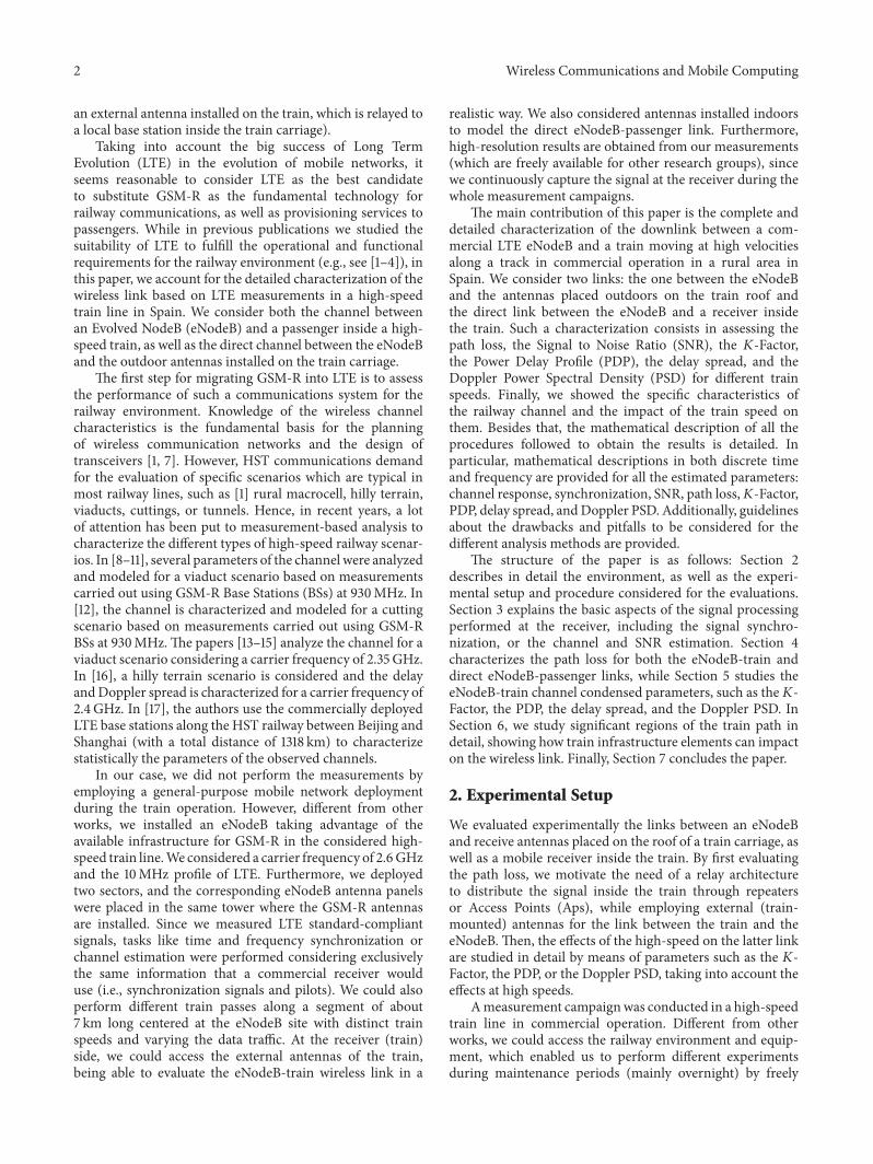
2 Wireless Communications and Mobile Computing
an external antenna installed on the train which is relayed toa local base station inside the train carriage)
Taking into account the big success of Long TermEvolution (LTE) in the evolution of mobile networks itseems reasonable to consider LTE as the best candidateto substitute GSM-R as the fundamental technology forrailway communications as well as provisioning services topassengers While in previous publications we studied thesuitability of LTE to fulfill the operational and functionalrequirements for the railway environment (eg see [1ndash4]) inthis paper we account for the detailed characterization of thewireless link based on LTE measurements in a high-speedtrain line in Spain We consider both the channel betweenan Evolved NodeB (eNodeB) and a passenger inside a high-speed train as well as the direct channel between the eNodeBand the outdoor antennas installed on the train carriage
The first step for migrating GSM-R into LTE is to assessthe performance of such a communications system for therailway environment Knowledge of the wireless channelcharacteristics is the fundamental basis for the planningof wireless communication networks and the design oftransceivers [1 7] However HST communications demandfor the evaluation of specific scenarios which are typical inmost railway lines such as [1] rural macrocell hilly terrainviaducts cuttings or tunnels Hence in recent years a lotof attention has been put to measurement-based analysis tocharacterize the different types of high-speed railway scenar-ios In [8ndash11] several parameters of the channel were analyzedand modeled for a viaduct scenario based on measurementscarried out using GSM-R Base Stations (BSs) at 930MHz In[12] the channel is characterized and modeled for a cuttingscenario based on measurements carried out using GSM-RBSs at 930MHzThe papers [13ndash15] analyze the channel for aviaduct scenario considering a carrier frequency of 235GHzIn [16] a hilly terrain scenario is considered and the delayandDoppler spread is characterized for a carrier frequency of24GHz In [17] the authors use the commercially deployedLTE base stations along the HST railway between Beijing andShanghai (with a total distance of 1318 km) to characterizestatistically the parameters of the observed channels
In our case we did not perform the measurements byemploying a general-purpose mobile network deploymentduring the train operation However different from otherworks we installed an eNodeB taking advantage of theavailable infrastructure for GSM-R in the considered high-speed train lineWe considered a carrier frequency of 26GHzand the 10MHz profile of LTE Furthermore we deployedtwo sectors and the corresponding eNodeB antenna panelswere placed in the same tower where the GSM-R antennasare installed Since we measured LTE standard-compliantsignals tasks like time and frequency synchronization orchannel estimation were performed considering exclusivelythe same information that a commercial receiver woulduse (ie synchronization signals and pilots) We could alsoperform different train passes along a segment of about7 km long centered at the eNodeB site with distinct trainspeeds and varying the data traffic At the receiver (train)side we could access the external antennas of the trainbeing able to evaluate the eNodeB-train wireless link in a
realistic way We also considered antennas installed indoorsto model the direct eNodeB-passenger link Furthermorehigh-resolution results are obtained from our measurements(which are freely available for other research groups) sincewe continuously capture the signal at the receiver during thewhole measurement campaigns
The main contribution of this paper is the complete anddetailed characterization of the downlink between a com-mercial LTE eNodeB and a train moving at high velocitiesalong a track in commercial operation in a rural area inSpain We consider two links the one between the eNodeBand the antennas placed outdoors on the train roof andthe direct link between the eNodeB and a receiver insidethe train Such a characterization consists in assessing thepath loss the Signal to Noise Ratio (SNR) the 119870-Factorthe Power Delay Profile (PDP) the delay spread and theDoppler Power Spectral Density (PSD) for different trainspeeds Finally we showed the specific characteristics ofthe railway channel and the impact of the train speed onthem Besides that the mathematical description of all theprocedures followed to obtain the results is detailed Inparticular mathematical descriptions in both discrete timeand frequency are provided for all the estimated parameterschannel response synchronization SNR path loss119870-FactorPDP delay spread andDoppler PSD Additionally guidelinesabout the drawbacks and pitfalls to be considered for thedifferent analysis methods are provided
The structure of the paper is as follows Section 2describes in detail the environment as well as the experi-mental setup and procedure considered for the evaluationsSection 3 explains the basic aspects of the signal processingperformed at the receiver including the signal synchro-nization or the channel and SNR estimation Section 4characterizes the path loss for both the eNodeB-train anddirect eNodeB-passenger links while Section 5 studies theeNodeB-train channel condensed parameters such as the119870-Factor the PDP the delay spread and the Doppler PSD InSection 6 we study significant regions of the train path indetail showing how train infrastructure elements can impacton the wireless link Finally Section 7 concludes the paper
2 Experimental Setup
We evaluated experimentally the links between an eNodeBand receive antennas placed on the roof of a train carriage aswell as a mobile receiver inside the train By first evaluatingthe path loss we motivate the need of a relay architectureto distribute the signal inside the train through repeatersor Access Points (Aps) while employing external (train-mounted) antennas for the link between the train and theeNodeB Then the effects of the high-speed on the latter linkare studied in detail by means of parameters such as the 119870-Factor the PDP or the Doppler PSD taking into account theeffects at high speeds
Ameasurement campaignwas conducted in a high-speedtrain line in commercial operation Different from otherworks we could access the railway environment and equip-ment which enabled us to perform different experimentsduring maintenance periods (mainly overnight) by freely
Wireless Communications and Mobile Computing 3
eNB
0 200 300100Instantaneous speed (kmh)
100 200 3000Instantaneous speed (kmh)
eNB
102
101
100
99
98
97
96
95
94
93
Kilo
met
ric p
oint
(km
)
Top speed 100 EGB Top speed 200 EGB
Figure 1 Map of the scenario considered for the measurementsThe instantaneous train speed is shown for each point of the trajectory bothfor the cases considering a maximum speed of 100 kmh and 200 kmh The position of the eNodeB is also specified Map Image by copy2017DigitalGlobe Cartography Institute of Andalucıa Map Data by copy2017 Google National Geographic Institute of Spain
controlling the train movement as well as the transmittedsignals Even more one of the most important features ofour experiments is that instead of using eNodeB deployedfor general-purpose mobile cellular communications weinstalled an eNodeB in one of the GSM-R sites specifi-cally devoted for railway communications Furthermore weobtained the permission to employ the carrier frequencyat 26GHz which is commercially used in such an areaMeasurements were carried out along a track segment ofapproximately 7 km long centered at the GSM-R site in arural area The considered train was specifically designed totest all the systems each time a new line is opened hencethe access to some resources such as the external antennasinstalled on its roof was granted This allowed us to analyzethe use of LTE for high-speed train applications at the actualenvironment and employing the specific infrastructure of therailway operator It is also worth noting that the transmitpower was high enough so that the SNR level exceeds20 dB (when using antennas placed outdoors) This allowsfor correctly synchronizing most of the LTE frames withouterrors hence enabling us to analyze the signal along thewholetrain path that is instead of only sampling the acquiredsignal during short time intervals while the train movesalong the track our equipment acquires the transmitted LTEframes in a continuous fashion The following subsectionsdescribe the details of the measurement environment theequipment used and the methodology followed to performthe measurements
21 Measurement Environment
211 Test Track The considered high-speed train line con-nects Cordoba and Malaga (Spain) and is designed to cope
with speeds up to 330 kmh The measured segment islocated between the Kilometric Points (KPs) 930 and 1020whereas the GSM-R site is located at KP 97075 (the exactGlobal Positioning System (GPS) coordinates of the site are37∘4101584031410158401015840N 4∘431015840125210158401015840W) as imaged in Figure 1 TheAntequera-Santa Ana Railway Station (KP 96800) and aTraffic Management Center are also located in the vicinity ofthe GSM-R site
212 Test Train The considered test train was the so-calledSeneca laboratory train (Talgo A-330) provided by the Span-ish Railway Infrastructure Administrator (ADIF) imagedin Figure 2(a) The train was intended for infrastructureinspections and it was extensively used in testing activitiesfor the deployment of the European Rail TrafficManagementSystemEuropean Train Control System (ERTMSETCS)standard in Spanish high-speed lines Electrically poweredthe train can reach a maximum speed of 363 kmh althoughthe maximum considered speed for our measurements waslimited to 200 kmh because the time (and also the distance)required to reach a higher speed is extremely large thuslimiting the number of trials to be performed in a typicalmeasurement session during the night The train is 8092mlong and includes an inner panel (see Figure 2(b)) whichallows for the connection to the external antennas on itsroof (see Figure 2(c)) two of them are multiband antennas(800 900 1800 1900 UMTS UMTSII W-LAN and GPS)Kathrein 870 10003 whereas the other two are Kathrein870 10007 (without GPS) both featuring a 0 dB gain anda Voltage Standing Wave Ratio (VSWR) smaller than 20 1at the considered carrier frequency of 26GHz During themeasurements we used two external antennas one of eachtype The GPS connection is used by the GPS-disciplined
4 Wireless Communications and Mobile Computing
(a) Photography of the whole train (b) Inner panel for con-nection to the outdoor an-tennas
(c) Outdoor antennas onthe roof of the train car-riage (Kathrein 870 10003and 870 10007) The fourantennas are marked withred ellipses
Figure 2 Seneca laboratory train (Talgo A-330)
(a) Image of the tower andthe two cabins for telecom-munications equipment
(b) Antenna installed at the tower (forsouth sector)
Figure 3 Pictures of the GSM-R site
oscillators included in the measurement equipment and tomatch the acquired samples with the estimated position andvelocity of the train
22 Measurement Equipment
221 Ground Equipment The GSM-R site imaged in Fig-ure 3(a) includes a 40m height tower with antennas fordifferent wireless technologies and two cabins where thecommunications equipment is installed A commercial LTEeNodeB was set up inside one of the available cabins and tworemote radio headsweremounted at the tower structure eachone connected to two antenna elements of a different antennapanel (see Figure 3(b)) Such antenna panels (Moyano MY-DTBSBS17276518) were placed at a height of 20m and ori-entated as the available GSM-R antennas At the consideredcarrier frequency (26GHz) these cross-polarized antennas
Table 1 Ground antennas orientation in both vertical (with respectto the horizontal plane) and horizontal (with respect to the northdirection) dimensions
Sector Antenna orientation [∘]Azimuth Elevation
North 355 0South 175 minus14
feature a gain of 18 dBi and a half-power beam width of62∘ (horizontal) and 5∘ (vertical) as imaged in the radiationpattern shown in Figure 4 Each antenna panel is used todeploy a sector hence two sectors are used named as ldquonorthsectorrdquo and ldquosouth sectorrdquo respectively (see Figure 1) Table 1shows the orientation of the ground antennas
Wireless Communications and Mobile Computing 5
Horizontal beamVertical beam
0∘
300∘
330∘
270∘
240∘
210∘
180∘150∘
120∘
90∘
60∘
30∘
minus6 >
minus3 >
Figure 4 Radiation pattern for the transmit antennas (MoyanoMY-DTBSBS17276518) Both the vertical and horizontal radiationpatterns are shown
The eNodeB was configured to transmit an LTE signalwith the profile of 10MHz bandwidth transmit diversity (asingle transmit block is encoded and transmitted throughtwo different antennas Precoding is performed in orderto separate the two different antennas) and normal cyclicprefix (CP) length (the first Orthogonal Frequency-DivisionMultiplexing (OFDM) symbol of an LTE slot (a slot occupieshalf a subframe) has a cyclic prefix length of 119873CP
long = 80samples (52083 microseconds) whereas for the remainingsix OFDM symbols the cyclic prefix is reduced to 119873CP
short =72 samples (46875 microseconds)) More details regardingthe transmit signal configuration are specified in Table 2Note that two configurations for data traffic transmissionwere considered (a commercial LTE receiver (different thanthose employed to produce the results shown in the paper)is connected as the only user to the eNodeB this way we cancapture the signals between the eNodeB and the commercialreceiver to be used for our evaluations)
(i) Maximum throughput all the resource blocks of theLTE signal are filled in with data Hence the max-imum payload of LTE is used for the configurationparameters specified in Table 2
(ii) ETCS + VoIP a stream of European Train ControlSystem (ETCS) data traffic is transmitted in parallelwith a Voice over Internet Protocol (VoIP) call
In both cases the receiver used in the measurements has noa priori knowledge about the transmit data
222 Onboard Equipment The onboard equipment consistsof two nodes from the so-called GTEC Testbed (described
Table 2 LTE testbed configuration parameters
Parameter ValueSampling frequency 119891119904 1536MHzTransmit power 46 dBmMaximum antenna gain 18 dBi (TX) 0 dBi (RX)Carrier frequency 26GHzBandwidth 10MHz (9MHz occupied)
Transmission scheme Transmission mode 2 (transmitdiversity) [18]
Cyclic prefix length Normal
in [19 20]) operating in receive-only mode Each of themincludes an EttusNational Instruments Universal SoftwareRadio Peripheral (USRP) B210 (see Figure 5(b)) board con-nected to a laptop running the GTEC 5G Simulator [20] (seeFigure 5(a)) and the Mathworks LTE Toolbox Notice thatthe source code of both the GTEC Testbed and the GTEC5G Simulator is publicly available under the GPLv3 license athttpsbitbucketorgtomas bolanogtec testbed publicgit [21]Whereas one of the nodes was connected to two exter-nal antennas available on the carriage roof the other wasconnected to two omnidirectional antennas (MobileMarkPSKN3-2455S) directly attached to theUSRP installed insidethe carriage The outdoor antennas allow us to evaluatethe link between the eNodeB and the train while theindoor ones are used to investigate the direct connectionbetween the mobile receiver of a passenger (or staff) andhow the eNodeB would work Additionally each nodewas provided with a GPS-disciplined temperature-controlledoscillator (EttusNational Instruments GPSDO 783454-01)that is also used for georeferencing (time and position)the measurements Given that the eNodeB also employsa GPS-disciplined oscillator the frequency offset betweenthe eNodeB and the GTEC Testbed nodes is minimizedNotice that whereas the USRP connected to the externalantennas uses theKathrein 870 10003GPS antenna theUSRPconnected to the indoor antennas uses a separate Trimble66800-40 GPS antenna which is also placed indoors
23 Measurement Procedure Different train passes wereperformed at different speeds in both north and southdirections considering different transmitter configurationsand different data traffic types GPS-based geolocation ofthe measurements allowed us to accurately combine theresults obtained from different train passes It is worth notingthat the obtained results exhibit a very high repeatabilitylevel for different train passes with identical configurationparameters This enables us to compare consistently theresults at different speeds It is also interesting to mentionthat we capture the data continuously at the receiver duringthe whole measurements session This not only requires ahuge amount of available storage (approximately 4 TB of rawdata for two measurement sessions of about 3 hours each)but also challenges the measurement equipment in termsof acquisition speed and stability demanding extremelypowerful hardware to process all the data In this sense also
6 Wireless Communications and Mobile Computing
(a) Two laptops mounted onboard running the GTEC5G Simulator as part of two GTEC Testbed nodes
(b) USRP employed as part ofa GTEC Testbed node equippedwith the indoor antennas Onlythe two antennas in the middleout of the four antennas are used
Figure 5 Onboard measurement equipment
the software developed has to be prepared to cope with such ahuge amount of data (details about these aspects can be foundin the description of our GTEC 5G Simulator and GTECTestbed in [20]) The main advantage of our approach is thatwe can obtain high-resolution results Additionally all ourmeasurement results are freely available for other researchgroups In order to have access to them please contact us attestbedgtecudces
231 Low SpeedMeasurements Train passes at 50 kmh wereperformed to characterize the propagation environment interms of large-scale parameters Hence the SNR and path lossfor the antennas placed indoors and outdoors were evaluatedFor these measurements we independently switched on andoff the two deployed sectors This enabled us to measure notonly the desired received power in a sector (eg receivedpower when the train is in the north sector and only thenorth sector is active) but also the interference caused to theadjacent sector (eg received power when the train is in thenorth sector and only the south sector is active)
The results presented along this paper were extractedfrom the samples acquired while the train speed was keptconstant (see Figure 1) whereas an overimposed pattern ofgray diagonal lines is used to emphasize the results obtainedwhile the train was accelerating or decelerating (see Figure 14as an example)
Figure 6 shows the average SNR per data subcarrierversus the KP In order to maximize the number of occupiedsubcarriers devoted to the SNR estimation the so-calledldquoMaximum Throughputrdquo is considered The SNR was eval-uated as described in Section 33 for one antenna placedindoors and another one placed outdoors It can be seenthat obviously the highest SNR values are obtained in thevicinity of the eNodeB When the train passes in front ofthe eNodeB the handover between the two sectors occursHowever the SNR is higher than 20 dB for all the points ofthe train trajectory when the outdoor antennas are used withthe maximum value being about 60 dBThe shape of the SNRcurves for the antennas placed indoors is similar although thereceived power decreases dramatically due to the penetrationlosses On average a loss of about 26 dB is measured
232 High-Speed Measurements Once the large-scale pa-rameters were characterized by means of low speed measure-ments measurements at higher velocities such as 100 kmh
eNodeB
Outdoorantenna
Indoorantenna
0
10
20
30
40
50
60
70
SNR
(dB)
96 98 100 10294
Kilometric point (km)
Figure 6 Estimated SNR versus KP for one of the indoor and oneof the outdoor antennas
and 200 kmh were performed This way we evaluated theeffect of the speed on parameters such as the 119870-Factor thePDP and the Doppler PSD Due to the time required toaccelerate and decelerate the train it was not possible tomeasure at high speeds during the whole train path Figure 1shows the instantaneous speed of the train versus the KP forbothmeasurements cases 100 kmh and 200 kmh As shownin Figure 1 the speed is maximum along the central part ofthe evaluated trajectory Even for the worst case (200 kmh)the evaluations are performed at the maximum speed at leastalong three kilometers In this case the considered modelfor the data traffic is the one labeled as ldquoETCS + VoIPrdquo inSection 221 However this does not affect the results sinceonly the pilots are used to perform the evaluations
3 Signal Processing at the Receiver
Several relevant parameters are estimated directly from theLTE-compliant acquired signal such as path loss PDP delayspread and Doppler PSD Most of the estimates depend onthe wireless channel response estimation which is done bymeans of the pilot symbols included in the LTE transmit
Wireless Communications and Mobile Computing 7
1 2 3 4 5 6 7 8 9 10
Slot 1 Slot 2
Band
wid
th =
62 +
DC
subc
arrie
rs
1
P-SC
H
6 7 1 7
Slot 11 Slot 12
1 6 7 1 7
10 ms (LTE FDD frame)
1ms (LTE subframe)
middot middot middot middot middot middot
middot middot middot
S-3
(1
P-SC
HS-3
(1
Figure 7 Synchronization signals for FDD LTE
signal In the following subsections we detail all the stepsfollowed to process the acquired signals in order to obtain theaforementioned estimates
31 Synchronization in LTE Before proceeding with thechannel response estimation the first step consists in detect-ing and synchronizing the LTE signal LTE provides two syn-chronization signals namely the Primary SynchronizationSignal (P-SCH) and the Secondary Synchronization Signal(S-SCH) to enable time and frequency synchronizationand to detect the physical cell ID which defines the pilotsequence as described in [22 Section 611] For FDD LTEsignalsmdashthe ones considered in our experimentsmdashthe P-SCH is transmitted by using the 62 central subcarriers of thelast OFDM symbol contained in the first and the eleventhslots of each LTE frame as shown in Figure 7This enables thereceiver to detect the P-SCH regardless of the configuration ofthe CP length Once the P-SCH is detected the signal is time-synchronized at slot level While the P-SCH is repeated twiceper LTE frame the S-SCH comprises two different signalsequences per each LTE frame being the first one transmittedin the 62 central subcarriers of the OFDM symbol previous tothe one used to transmit the first copy of the P-SCH whereasthe second one is located at the OFDM symbol precedingthe one used to transmit the second copy of the P-SCH (seeFigure 7) Hence once detected the S-SCH the signal is time-synchronized at LTE frame level Given that only the central62 subcarriers are employed for synchronization the receivercan synchronize with no a priori knowledge of the total signalbandwidth
The P-SCH is constructed from a frequency-domainZadoff-Chu sequence of length 63 [23] Among its propertiesthe ability to detect it even with a frequency offset upto plusmn75 kHz is highlighted Hence the time offset can beestimated initially without requiring to perform a frequencysynchronization (notice also that both the eNodeB and theGTEC Testbed nodes use GPS-disciplined oscillators thusthe frequency offset between them is very small) On theother hand the S-SCH sequence is based onmaximum lengthsequences known as 119872-sequences [23] Since the S-SCH isdetected after the P-SCH the P-SCH itself can be used toperform a rough channel response estimation to aid in thedetection of the S-SCH [23]
Table 3 LTE signal configuration parameters
Parameter Notation ValueOFDM symbols per frame 119904119865 140Samples per frame 119904119878119865 153600Samples per slot 119904119878slot 7680FFT size 119873 1024 pointsNumber of used subcarriers 119873119906 600OFDM symbols per LTE slot 119873slot 7Long CP length 119873CP
long 80 samplesShort CP length 119873CP
short 72 samplesMean CP length 119873CP asymp7314 samples
Since our environment comprises two different sectorseach of them having a different physical cell ID we can easilydetermine both the P-SCH and the S-SCH sequences persector Hence both of them can be found by using a simplecorrelation thus acquiring the symbol and LTE frame timing
32 Channel Response Estimation The wireless channelresponse between the eNodeB and the receiver is estimated bytaking advantage of the pilot structure defined by LTE Firstlyan estimate of the discrete-time frequency-domain channelresponse 119897[119899 120582] is obtained for each LTE frame 119897 ge 0 where119899 = 0 119904119865 minus 1 denotes the OFDM symbol index with119904119865 being the number of OFDM symbols per LTE frame and120582 = minus1198732 1198732minus1 the subcarrier index with119873 being theFast Fourier Transform (FFT) size of the OFDM modulatorWe used a Minimum Mean Squared Error (MMSE) channelestimator Refer to Table 3 for the definition of the constantsemployed in this section
Notice that frequency synchronization is skipped sinceone of the parameters that we are estimating is the DopplerPSD and this process will be altered due to the correctionsintroduced by the frequency synchronization algorithmsThe estimated channel response in the discrete-time domainfor the 119897th frame namely ℎ119897[119899 120581] is obtained by applyingthe Inverse Fast Fourier Transform (IFFT) operation to
8 Wireless Communications and Mobile Computing
the corresponding discrete-time frequency-domain channelresponse as
ℎ119897 [119899 120581] = IFFT120582 (119897 [119899 120582]) (1)
where IFFT120582(sdot) denotes the IFFT operation over 120582 and 120581 =minus1198732 1198732 minus 1 is the discretized delay index Note thatthe channel seen by the signal comprises subcarriers withindices 120582 = minus119873119906 119873119906 However the MMSE channelestimator provides an estimation of the channel response forthe 119873 subcarriers considered (ie it also includes the guardsubcarriers)This enables us to avoid the spreading effect thatwould appear if guard subcarriers are set to zero due to theproperties of the IFFT
Since the LTE frames are transmitted in a continuousfashion (ie there are no gaps or silent periods betweenconsecutive LTE frames) we can obtain an estimation ofthe wireless channel response along the train path namelyℎ[119899 120581] by concatenating the estimates of successive LTEframes However for doing so the propagation delay andthus the synchronization points (a synchronization point isdefined as the index of the first sample of the acquired signalcorresponding to a valid LTE frame) must be taken intoaccount
The synchronization point for the 119897th LTE frame (seeSection 31 for more details about the synchronization proce-dure) namely 119901119897 can be expressed as a function of the frameindex 119897 as
119901119897 = 119899119894 + 119897 sdot 119904119878119865 + 120574119897 (2)
being
120574119897 = lfloor120591119897 sdot 119891119904rceil + 119890119897 (3)
where 119899119894 is the index of the initial sample for the firsttransmitted LTE frame 119904119878119865 is the number of samples perLTE frame 120591119897 is the propagation delay for the 119897th framewhich depends on the distance between the receive antennamounted on the train and the transmit antenna at theeNodeB lfloorsdotrceil denotes the round operation 119891119904 is the samplingfrequency and 119890119897 is an integer error term which depends onthe actual channel and the noise
The detected synchronization point 119901119897 allows us to com-pensate for the propagation delay in the estimated channelresponses hence centering the most powerful tap around120581 = 0 For the case of two consecutive frames 119897 and 119897 + 1being synchronized if Δ120574119897 ≜ 120574(119897+1) minus 120574119897 = 0 there will be adiscontinuity in the estimated channel responses between thetwo frames (note that Δ120574119897 = 119901(119897+1) minus 119901119897 minus 119904119878119865) The continuitycan be preserved by accounting for the propagation delay ofthe received frames This can be done since the IFFT sizein (1) equals the number of subcarriers thus the samplingtime of the signal and the estimated channel delays match Topreserve the continuity we can follow different strategies
321 Synchronizing Only the First Frame We can takeadvantage of the OFDM cyclic prefix (CP) and synchronizeonly the first frame Then instead of synchronizing each
0
2
4
6
8
10
12
14
minus2
Delay for each frameRegression line fit
800200 300 400 500 600 700100 9000Frame index (l)
Del
ay (
l ) (sa
mpl
es)
Figure 8 Exemplary results of delays (120581119897) for a portion of thecaptured frames
successive LTE frame (hence obtaining the synchronizationpoints defined in (2)) the synchronization point for the 119897thframe is obtained as 119901119897 = 119899119894+119897 sdot 119904119878119865 without accounting for thepropagation delayThis way the overall channel response (iethe concatenation of the channel responses for the subframesalong the whole path) is defined as
ℎ [119899 120581] = ℎ119897 [119899 minus 119904119865 sdot 119897 120581 minus 1205810] 119897 = lfloor 119899119904119865rfloor (4)
where lfloorsdotrfloor is the floor operator and 1205810 is the delay of the firstsynchronized frame
This method is only valid when the propagation delayis relatively small compared to the CP length otherwiseIntersymbol Interference (ISI) will arise in the signal
322 Synchronize Each Frame and Find Relative DelaysWhen synchronizing all the frames we obtain the synchro-nization points defined in (2) The corresponding delayexpressed as the number of samples for the 119897th frame namely120581119897 is
120581119897 = 1205810 +119897minus1
sum119898=0
Δ120574119897 (5)
where 1205810 is the delay (expressed in number of samples) forthe first synchronized frame Therefore the overall channelresponse is
ℎ [119899 120581] = ℎ119897 [119899 minus 119904119865 sdot 119897 120581 minus 120581119897] 119897 = lfloor 119899119904119865rfloor (6)
Figure 8 shows some exemplary results for the obtained delaysamples 120581119897 versus the frame number 119897 considering 1205810 = 0
Wireless Communications and Mobile Computing 9
These results correspond to a portion of the captured framesfor the case of the train moving away from the eNodeB ata speed of 100 kmh We also show the fitting of the dataobtained by a robust linear regression [24] The slope ofthe curve shows how the propagation delay increases as theframes are received while the train moves away from theeNodeB thus increasing the distance between transmit andreceive antennas
323 Hybrid Approach We can use a hybrid approach fromthe two above-mentioned methods Firstly the acquiredsignals are grouped in sets of consecutive frames Secondlythe channel response is estimated for each set as explainedin Section 321 Then the propagation delays are estimatedfor each set following a procedure similar to the one inSection 322
The initial time (in seconds) corresponding to the esti-mated channel response ℎ[119899 120581] for each value of 119899 namely119905119899 can be approximated as
119905119899 ≃ 119899 1119891119904 (119873 + 119873CP) + 0 (7)
where 0 is the initial time of the estimated channel responsefor the symbol with 119899 = 0 and
119873CP = (119873slot minus 1)119873CPshort + 119873CP
long
119873slot(8)
is the mean number of samples of the CP within the LTEframe where 119873CP
long and 119873CPshort are the lengths of the long and
short LTE CP and119873slot is the number of OFDM symbols perslot Notice that the equality in (7) holds if 119899mod119873slot = 0
The delay (in seconds) corresponding to the estimatedchannel response ℎ[119899 120581] for each value of 120581 namely 120591120581 isobtained as
120591120581 = 120581119891119904 (9)
Note that it is possible to obtain an exact expression for 119905119899 as119905119899 = 1
119891119904 (lfloor 119899119873slot
rfloor 119904slot + 119906slot (119899mod119873slot)) + 0 (10)
where
119906slot (119898)= [119873CP
long + 119873 + (119873CPshort + 119873) (119898 minus 1)] (1 minus 1205751198980)
(11)
is the index of the starting sample of the 119898th OFDM symbolwithin an LTE slot 119904119878slot is the number of time-samples perLTE slot and 120575119901119902 is the Kronecker delta function defined as
120575119894119895 =
1 if 119894 = 1198950 if 119894 = 119895 (12)
For many of the estimations performed in the followingsections (eg see Section 5) it is more convenient to consider
a channel with an impulse response starting at delay zerofor all 119899 namely ℎ[119899 120581] This allows us to consider thesame subset of delays (when estimating parameters from thechannel (see Section 5) we use a finite number of delays lessthan119873CP
short) along the whole path for estimating each desiredparameter Therefore we estimate the propagation delay foreach frame 119897 as the number of samples including a fractionalpart namely 120581119897 = 120581119897119894 + 120581119897119891 where 120581119897119894 is the integer part and120581119897119891 is the fractional one Then we can estimate the channelresponse for the 119897th frame correcting the fractional part as
ℎ119897 [119899 120581] = IFFT119873120582 (119897 [119899 120582] sdot 119890minus1198952120587(120582119873)120581119897119891) (13)
The integer part is compensated by applying an offset tothe delay when obtaining the complete channel response thatis
ℎ [119899 120581] = ℎ119897 [119899 minus 119904119865 sdot 119897 120581 minus 120581119897119894] 119897 = lfloor 119899119904119865rfloor (14)
33 SNR Estimation The SNR is estimated consideringexclusively the data subcarriers by means of the methoddescribed in [1 Section 452] Guard subcarriers DirectCurrent (DC) subcarrier and pilot subcarriers are discardeda priori Hence the average SNR per data subcarrier isobtained The SNR estimation is performed by consideringthe following steps
(1) Noise samples in the time domain are captured withthe transmitter switched off (hence not transmittingany signal)
(2) The captured noise samples in the time domain arethen processed as if they were actual data samplesthat is the cyclic prefix is removed a FFT is per-formed and both guard and DC subcarriers areremoved
(3) As a result 119908(119899120582) noise samples are obtained in thefrequency domain each one corresponding to the120582th subcarrier of the 119899th OFDM symbol where 120582 isinD(119899) with D(119899) being the set of indexes of the datasubcarriers for the 119899th OFDM symbol
(4) All previous steps are repeatedwhen the transmitter isswitched on so 119903(119899120582) data samples (of course affectedby noise) are obtained in the frequency domain
(5) The average SNR for each OFDM symbol is thenestimated by averaging out the instantaneous SNRvalues for the different data subcarriers Define
119903(119899) = 11003816100381610038161003816D(119899)1003816100381610038161003816 sum120582isinD(119899)
10038161003816100381610038161003816119903(119899120582)100381610038161003816100381610038162
119908(119899) = 11003816100381610038161003816D(119899)1003816100381610038161003816 sum120582isinD(119899)
10038161003816100381610038161003816119908(119899120582)100381610038161003816100381610038162
(15)
10 Wireless Communications and Mobile Computing
where |D(119899)| is the cardinality of D(119899) that is thenumber of data subcarriers for the 119899th symbol Thenthe SNR for each OFDM symbol is calculated as
SNR(119899) = 119903(119899) minus 119908(119899)119908(119899) (16)
4 Path Loss Estimation
The path loss is defined as the ratio between the transmittedand the received power and it is expressed in decibels as afunction of the distance as [25]
PL (119889) = 10 log10 119875119905119875119903 (119889) (17)
where PL(119889) is the path loss (in dB) for a distance 119889 119875119905is the transmit power and 119875119903(119889) is the receive power at adistance 119889 In this manuscript we adopt a simplified log-distance path loss model which allows us to characterize thelarge-scale path loss as well as the shadow fading variationsof the channel response This model is expressed as in [25]
PL (119889) = PL (1198890) + 10120574 log10 ( 1198891198890) + 119883120590
= 119887 + 10120574 log10119889 + 119883120590(18)
where 120574 is the so-called path loss exponent 1198890 is a distancerelatively close to the transmitter known as ldquobreak distancerdquoor ldquobreakpointrdquo119883120590 is a zero-meanGaussian randomvariablewith a standard deviation 120590 representing the variations due tothe medium and small-scale fading and PL(1198890) correspondsto the mean path loss at the break distance The termsdepending on 1198890 are reorganized to obtain the last expressionin (18)
Using (18) (neglecting 119883120590) we estimate 119887 and 120574 for eachcombination of active sector receive antenna and measuredsector by using least-squares fitting over the energy of thereceive signal (note that the low speed measurements asexplained in Section 23 are used here) This way we obtainthe large-scale fading curves for each scenario Figures 9 and10 show the received energy for both sectors when only asingle sector was active Note that only the results for outdoorantenna 1 and indoor antenna 1 are shown in all the plotsthe results for the other antennas are similar For each energycurve the corresponding fitting is provided As shown inFigures 9 and 10 for the highest and the lowest considereddistance values themodel does not fit well the data due to thehigh directivity of the transmit antennas This is because theomnidirectional model assumed for the transmit antennasdoes not hold in this case Figures 9 and 10 also show that theantennas serving the north sector cause interference into thesouth sector and vice versa This is due to the configurationof the eNodeB antennas
Given that 119883120590 is modeled as a zero-mean Gaussianrandom variable with standard deviation 120590 we subtract theobtained fittings from the received energies to estimate sucha standard deviation 120590 Figures 11 and 12 show the estimatedcumulative probabilities of 119883120590 when only a single sector
0
10
20
30
40
50
60
Rece
ived
pow
er (d
B)
22 24 26 28 3 32 34 36 382
North outdoorsNorth indoors
South outdoorsSouth indoors
FIA10 m)Distance (
Figure 9 Received energy and least-squares fitting along both northand south sectors for the receive outdoor antenna 1 and the receiveindoor antenna 1 Only the antennas serving the north sector weretransmitting
22 24 26 28 3 32 34 36 382
0
10
20
30
40
50
60
Rece
ived
pow
er (d
B)
South outdoorsSouth indoors
North outdoorsNorth indoors
FIA10 m)Distance (
Figure 10 Received energy and least-squares fitting along bothnorth and south sectors for the receive outdoor antenna 1 and thereceive indoor antenna 1 Only the antennas serving the south sectorwere transmitting
(north or south) is active We also plot the theoretical cumu-lative probabilities of zero-mean Gaussian distributions withthe standard deviation 120590 estimated for each case We can seethat the fitting between the estimated and theoretical curvesis very good Finally Table 4 shows the corresponding pathloss parameters (120574 119887 and120590) estimated from themeasurementdata
As seen in Table 4 the path loss exponent is verysimilar for all cases (both sectors as well as indoor and
Wireless Communications and Mobile Computing 11
Outdoor antenna 1
North sector South sector
Indoor antenna 1
0
02
04
06
08
1
minus5 0 5 10minus10
X (dB)
(0 276)(0 384)North sector South sector
(0 244)(0 317)
minus5 0 5 10minus10
X (dB)
P(X
lt
<M=CM)
Figure 11 Cumulative probabilities for receive outdoor antenna 1 and indoor antenna 1 along both north and south sectors Only the antennasserving the north sector were transmitting
Table 4 Path loss parameters (120574 119887 and 120590) estimated for both north (N) and south (S) sectors and for each of the four receive antennas twoof them are placed inside the train car (ldquoindoor ant 1rdquo and ldquoindoor ant 2rdquo) and the other two are placed outdoors on the train roof (ldquooutdoorant 1rdquo and ldquooutdoor ant 2rdquo) The results are obtained considering a single active sector (north or south) that is the sector whose antennasare transmitting The column TX specifies the active sector whereas the column RX denotes the sector along which the measurements areperformed
TX RX Outdoor ant 1 Outdoor ant 2 Indoor ant 1 Indoor ant 2120574 119887 120590 120574 119887 120590 120574 119887 120590 120574 119887 120590
N N 320 13561 384 253 11334 408 333 12088 318 317 11593 285S 223 7863 276 180 6494 183 120 3694 438 074 2675 106
S N 206 7844 191 223 7870 178 182 5816 209 189 6096 156S 229 11000 374 232 10336 168 264 10089 270 258 9891 239
outdoor receive antennas) However a large penetrationloss is observed for the indoor receiver This justifies theutilization of a relay scheme for provisioning services to theusers in a practical deployment Hence for the rest of theanalysis we consider exclusively the external link (eNodeBto outdoor antennas)
5 Estimation of ChannelCondensed Parameters
The so-called condensed parameters allow us to characterizeother effects of the channel different than the path loss In thissection we consider condensed parameters like 119870-FactorPDP delay spread and Doppler PSD
51 119870-Factor The evaluated scenario can be classified asrural area and exhibits a strong Line-of-Sight (LoS) compo-nent during most of the train trajectory Thus one of thechannel paths presents a predominant power with respect to
the others Due to this the fluctuations of the path gain followa Rice distribution The Rice distribution is parametrized bythe power ratio of the fixed and fluctuating components of thepath loss namely the119870-Factor
The instantaneous values of the 119870-Factor are calculatedaccording to the method proposed by Greenstein et al in[26] More specifically [26 Eq (9)] was evaluated for theexperimental data taking into account the tap correspondingto the LoS component
Figures 13 and 14 show the instantaneous values of the119870-Factor expressed in decibels versus theKP for the train speedsof 100 kmh and 200 kmh respectively Smoothed values ofthe 119870-Factor by using a sliding window are also plotted insuch figures The obtained results show that the 119870-Factoris noticeably higher than zero which is coherent with thehypothesis of the existence of a strong LoS component Onlyat certain positions along the train trajectory the 119870-Factorexhibits deep local minimum values (eg at KPs 966 km and984 km) which are caused by reflecting obstacles along the
12 Wireless Communications and Mobile Computing
Outdoor antenna 1
North sector South sector
Indoor antenna 1
0
02
04
06
08
1P
(Xlt
<M=CM)
minus5 0 5 10minus10
X (dB)
(0 374)(0 192)North sector South sector
(0 270)(0 209)
minus5 0 5 10minus10
X (dB)
Figure 12 Cumulative probabilities for receive outdoor antenna 1 and indoor antenna 1 along both north and south sectors Only the antennasserving the south sector were transmitting
Instantaneous K-Factor valuesSmoothed K-FactoreNodeB position
96 97 98 99 10095Kilometric point (km)
minus10
minus5
0
5
10
15
20
25
30
K-F
acto
r (dB
)
Figure 13 Estimated 119870-Factor for outdoor antenna 1 for the trainmoving at 100 kmh from the north sector to the south one Bothsectors are active The results of averaging out the instantaneousvalues by means of a sliding window are also shown
train path (see Section 6 for more details) It can be also seenthat the trend of the 119870-Factor does not change significantlywith the train speed
52 Power Delay Profile A parameter typically used toanalyze howmuch energy arrives at the receiverwith a certaindelay is the PDPThe PDP around the 119899th OFDM symbol can
Instantaneous K-Factor valuesSmoothed K-FactoreNodeB position
96 97 98 99 10095Kilometric point (km)
minus10
minus5
0
5
10
15
20
25
30
K-F
acto
r (dB
)
Figure 14 Estimated 119870-Factor for outdoor antenna 1 for the trainmoving at 200 kmh from the north sector to the south one Bothsectors are active The overimposed pattern of gray diagonal linesdenotes the areas where the train speed was not constantThe resultsof averaging out the instantaneous values by means of a slidingwindow are also shown
be obtained from a complex-valued channel time responseestimate as in [27]
119875 [119899 120581] = 12120572 + 1
119899+120572
sum119898=119899minus120572
10038161003816100381610038161003816ℎ [119898 120581]100381610038161003816100381610038162 (19)
Wireless Communications and Mobile Computing 13
18
16
14
12
10
8
6
4
2
0
Del
ay (
s)
95 96 97 98 99 100
Kilometric point (km)
50
60
70
80
90
100
110
PDP
(dB)
Figure 15 Estimated PDP for outdoor antenna 1 for the trainmoving at 100 kmh from the north sector to the south one Bothsectors are active
where 120572 adjusts the length of the considered segment of thetime response (the considered segment includes the timeresponses for the OFDM symbols whose indexes are 119899 minus120572 119899 + 120572)
Figures 15 and 16 show the estimated PDP for the trainmoving at 100 kmh and 200 kmh respectively with bothsectors being active The presented results are obtained byevaluating (19) for equally spaced OFDM symbols Note thatthe shape of the PDP curves accounts for the propagationdelay where the values with the lowest delay are the onescorresponding to the KPs closer to the transmit antennaNote also that the magnitude of the PDP decreases with thedistance to the eNodeB antennas
By comparing Figures 15 and 16 we can conclude that thePDP is independent from the train speed It is important tonote that the longer PDP responses around the eNodeB arecaused by the energy spreading effect of the IFFT This effectis not so noticeable for other KPs since their power is muchlower
Results corresponding to the trainmoving at 100 kmh areshown in Figure 17 when the propagation delay is subtractedthat is we evaluate (19) by using ℎ[119899 120581] instead of ℎ[119899 120581]for equally spaced OFDM symbols Furthermore the valuesobtained per frame were normalized hence the magnitudeobtained does not depend on the distance to the transmitantennaThis way we can perform a fair comparison betweenthe PDP results for different KPs not taking into account theenergy spreading effect of the IFFT It can be seen that PDPresponses are noticeable longer for some areas (eg at KPs966 km and 984 km) which is caused by reflecting obstaclesalong the train path (see Section 6 for more details)
It has been shown that under some specific circumstancesthe error probability due to delay dispersion is proportionalto the normalized second-order central moment of the PDPnamely the RMS delay spread [27] RMS delay spread can becalculated as
120590120581 [119899] = radic1205912120581 [119899] minus (120591120581 [119899])2 (20)
18
16
14
12
10
8
6
4
2
0
Del
ay (
s)
95 96 97 98 99 100
Kilometric point (km)
50
60
70
80
90
100
110
PDP
(dB)
Figure 16 Estimated PDP for outdoor antenna 1 for the trainmoving at 200 kmh from the north sector to the south one Bothsectors are active
95 96 97 98 99 100
Kilometric point (km)
minus1
0
1
2
3
4D
elay
(s)
minus50
minus45
minus40
minus35
minus30
minus25
minus20
minus15
minus10
minus5
PDP
(dB)
Figure 17 Normalized PDP for outdoor antenna 1 for the trainmoving at 100 kmh from the north sector to the south one nottaking into account the propagation delay Both sectors are active
where the second moment of 120591120581 is given by
1205912120581 [119899] = sum120581 119875 [119899 120581] 1205912120581sum120581 119875 [119899 120581] (21)
and the first one is obtained as
120591120581 [119899] = sum120581 119875 [119899 120581] 120591120581sum120581 119875 [119899 120581] (22)
Figures 18 and 19 show the RMS delay spread for equallyspaced OFDM symbols for the train moving at 100 kmh and200 kmh respectively The plots also include the results ofsmoothing out the instantaneous RMS delay spread values bymeans of a sliding window as well as the mean delay spreadfor the whole path followed by the train In Figures 18 and 19we can see that the delay spread results are coherent regardlessof the considered speed Results shown in Figures 18 and 19are congruent with those in Figure 17 showing a larger delayspread for the areas with more reflections
14 Wireless Communications and Mobile Computing
0
01
02
03
04
05
06
Dela
y sp
read
(s)
Instantaneous valueSmoothed value
Mean valueeNodeB position
96 97 98 99 10095Kilometric point (km)
Figure 18 Estimated RMS delay spread for outdoor antenna 1 forthe train moving at 100 kmh from the north sector to the southone Both sectors are active A curve corresponding to smoothedinstantaneous values by means of a sliding window are also shownas well as the mean delay spread for the whole path
0
01
02
03
04
05
06
Dela
y sp
read
(s)
Instantaneous valueSmoothed value
Mean valueeNodeB position
96 97 98 99 10095Kilometric point (km)
Figure 19 Estimated RMS delay spread for the train moving at200 kmh from the north sector to the south one Both sectorsare active The overimposed pattern of gray diagonal lines denotesthe areas where the train speed was not constant Smoothedinstantaneous values by means of a sliding window are also shownas well as the mean delay spread for the whole path
53 Doppler Power Spectral Density The Doppler PowerSpectral Density is related to the Angle of Arrivals (AoAs) ofthe multipath components and the direction of movement ofthe receiver Doppler PSD around the 119899th OFDM symbol forthe delay index 120581 namely 119878[119899 120581 120579] can be obtained as theFFT of the autocorrelation of a certain segment of the timeresponse of the channel centered at time index 119899 Considering
95 96 97 98 99 100
Kilometric point (km)
minus60
minus50
minus40
minus30
minus20
minus10
Dop
pler
PSD
(dB)
minus400
minus300
minus200
minus100
0
100
200
300
400
Dop
pler
freq
uenc
y (H
z)
Figure 20 Doppler Spectrum for outdoor antenna 1 for the trainmoving at 100 kmh from the north sector to the south one withboth sectors being active
the estimated channel response ℎ[119899 120581] the autocorrelationvalues are obtained as
119877ℎ [119899 120581 120582] =
119899+2120572minus120582
sum119898=119899
ℎ [119898 + 120582 120581] ℎlowast [119898 120581] 120582 ge 0119899+2120572+120582
sum119898=119899
ℎ [119898 120581] ℎlowast [119898 + 120582 120581] 120582 lt 0(23)
where 120582 = minus2120572 2120572 is the lag of the autocorrelation and120572 adjusts the length of the considered segment of the channeltime responseThen theDoppler scattering function [27] canbe written as
119878 [119899 120581 120579] = FFT120582 119877ℎ [119899 120581 120582] (24)
where FFT120582sdot denotes the FFT of the argument with respectto the autocorrelation lag 120582 and 120579 is the discretized Dopplerfrequency index being the correspondingDoppler frequency
]120579 = 120579 119891119904119873 + 119873CP
119873corr119873119863 (25)
where 119873corr = 4120572 + 1 is the number of samples ofthe autocorrelation 119873119863 is the size of the FFT and 120579 =minus1198731198632 1198731198632 minus 1 Note that (119873 + 119873CP)119891119904 is the meanduration of anOFDMsymbolTheDoppler PSD 119878 is obtainedafter averaging out the Doppler scattering function 119878 over 120581values as
119878 [119899 120579] = 1|K| sum120581isinK
119878 [119899 120581 120579] (26)
whereK denotes the set of considered values for 120581Figures 20 and 21 show the normalized Doppler PSD
for equally spaced OFDM symbols when the train moves at100 kmh and 200 kmh respectively obtained as indicated in(26) As expected themodule of themaximumDoppler valueis related to the train speed as
1003816100381610038161003816119891max1003816100381610038161003816 asymp |V| 119891119888
1198880 (27)
Wireless Communications and Mobile Computing 15
95 96 97 98 99 100
Kilometric point (km)
minus60
minus50
minus40
minus30
minus20
minus10
Dop
pler
PSD
(dB)
minus800
minus600
minus400
minus200
0
200
400
600
800
Dop
pler
freq
uenc
y (H
z)
Figure 21 Doppler Spectrum for outdoor antenna 1 for the trainmoving at 200 kmh from the north sector to the south one withboth sectors being active The overimposed pattern of gray diagonallines denotes the areas where the train speed was not constant
where 119891max denotes the maximum Doppler frequency V thevelocity of the train and 119891119888 = 26GHz the carrier frequencyThis brings us to maximum Doppler PSD values of approx-imately 2407Hz and 4805Hz for train speeds of 100 kmhand 200 kmh respectively The sign of the instantaneousDoppler PSD values depends on the direction of the velocityvector of the train with respect to the transmitterThis causesthe effect shown in Figures 20 and 21 where the Doppler PSDvalues concentrate around plusmn|119891max| and change abruptly whenthe train passes by in front of the eNodeB antennas
When the train is in the north sector (ie it approachesthe eNodeB) the Doppler PSD is maximum in +|119891max| Con-versely when the train is in the south sector (iemoving awayfrom eNodeB) the Doppler PSD reaches its maximum atminus|119891max|This is coherent with themeasurement environmentwhich features a strong LoS component However significantreflections in minus|119891max| for the north sector (conversely valuesin +|119891max| for the south sector) can be seen which are causedby obstacles along the train path (see Section 6 for moredetails)
6 Particularities of theMeasured Train Scenario
In the previous section we showed different condensedparameters along the whole train trajectory However sincethe total distance shown is relatively large small detailscannot be appreciated In this section we show and discussthe PDP and the Doppler PSD for three specific segments ofthe train trajectory each of them being 250m long which areas follows
(i) Segment (a) KPs between 98375 and 98625 Thereare strong reflections in this area as shown by theDoppler results in Figures 20 and 21 Also the 119870-Factor achieves the lowest values and the delay spreadthe highest ones in this area (see Figures 13 and 14for the 119870-Factor and Figures 18 and 19 for the delay
spread)This supports the hypothesis of a weaker LoScondition
(ii) Segment (b) KPs between 98875 and 99125 In thisarea the 119870-Factor and the delay spread take valuesclose to themean ones shown in Figures 13 and 14 andin Figures 18 and 19 respectively
(iii) Segment (c) KPs between 10025 and 1005 In thisarea the119870-Factor achieves the highest values and thedelay spread the lowest ones (see Figures 13 and 14for the 119870-Factor and Figures 18 and 19 for the delayspread)
Figure 22 shows the Doppler Spectrum for the threeaforementioned segments when the train moves at 100 kmhFor all the segments shown the train moves away from theeNodeB within the south sector therefore the LoS Dopplercomponent is located approximately at minus|119891max| = minus2407Hz(see Section 53) Furthermore a noticeable reflection com-ponent can be seen in the opposite frequency +|119891max| =2407Hz In addition abrupt transitions in the Doppler fromminus|119891max| to +|119891max| occur periodically These transitions in theDoppler are similar to the ones occurring when the trainpasses by in front of the eNodeB antennas (see Figures 20and 21) In fact these abrupt changes in the Doppler are dueto the nearby objects reflecting the signal More specificallythe masts supporting the overhead line (see Figure 26(b))are the origin of the stronger reflections It can be seen thatthe distance between consecutive masts (see Figure 26(a)) iscoherent with the separation between consecutive Dopplertransitions shown in Figure 22 Finally it is worth noting thatthemagnitude of the reflected componentswith respect to theLoS component depends on the position of the train along thepath This is related both to the distance and the angle withrespect to the transmit antenna
Figure 23 shows the normalized PDP for the threesegments verifying the existence of reflection componentscoherent with those shown in Figure 22 The PDP figuresclearly show that the reflected component associated witheach mast decreases its delay with respect to the LoS compo-nent (and increases its power) when the train moves towardsto the mast The magnitude of the reflected componentswith respect to the LoS one is coherent with the relationshipbetween the reflected component and the LoS one shown inFigure 22 For example the largest reflections in the PDP areobtained for the segment (a) Coherently the magnitude ofthe reflectionswith respect to the LoS component in Figure 22is also maximum for the segment (a)
It is important to notice that the described effects areindependent of the train speed Figure 25 shows the normal-ized Doppler PSD and the normalized PDP for the segment(a) when the train moves at 200 kmh
Figure 24 shows the estimated Doppler PSD for the threeconsidered segments Note that the regular oscillations inthese results are a manifestation of the Gibbs phenomenonafter evaluating (24) due to the use of time-limited signalsto calculate (23) In agreement with Figure 22 the maximumof the Doppler PSD is located in minus|119891max| (due to the con-tribution of the main path) For the segments with strongerreflected components a relevant peak is also appreciated in
16 Wireless Communications and Mobile Computing
984 9845 985 9855 986
Kilometric point (km)
minus50
minus40
minus30
minus20
minus10
Dop
pler
PSD
(dB)
minus400
minus300
minus200
minus100
0
100
200
300
400
Dop
pler
freq
uenc
y (H
z)
(a) Doppler Spectrum for the train moving at 100 kmh along the segment(a)
989 9895 99 9905 991
Kilometric point (km)
minus50
minus40
minus30
minus20
minus10
Dop
pler
PSD
(dB)
minus400
minus300
minus200
minus100
0
100
200
300
400
Dop
pler
freq
uenc
y (H
z)
(b) Doppler Spectrum for the train moving at 100 kmh along the segment(b)
10025 1003 100410035 10045 1005
Kilometric point (km)
minus400
minus300
minus200
minus100
0
100
200
300
400
Dop
pler
freq
uenc
y (H
z)
minus50
minus40
minus30
minus20
minus10
Dop
pler
PSD
(dB)
(c) Doppler Spectrum for the train moving at 100 kmh along the segment(c)
Figure 22 Doppler Spectrum for outdoor antenna 1 for the train moving at 100 kmh along the segments (a) (b) and (c)
+|119891max| The magnitude of the peak with respect to the maincomponent is reduced for the cases with lower reflectionsFor other frequencies the Doppler values are distributedapproximately according to a ldquoUrdquo shape This suggests thatalthough there is a strong LoS in the railway environmentreflections caused by railway infrastructure elements maylead to a Doppler PSD with noticeable components in otherfrequencies similar to the Jakes spectrum [28] It is worthnoting that the condensed parameters are affected by thereflections as they noticeably change their respective trendsin the areas where the reflections are stronger (eg segment(a)) Due to this we can expect severe effective link SNRdegradation for such areas
Note that the obtained results match those shown in [15]obtained for a similar test environment Finally Figure 25(c)shows the estimated Doppler PSD for the segment (a)when the train moves at 200 kmh The obtained results arecoherent with those corresponding to a moving speed of100 kmh
7 Conclusions
In this paper we provided a complete and detailed char-acterization of the downlink (Long Term Evolution (LTE)Frequency-Division Duplex (FDD) for the 10MHz profile)between a commercial LTE Evolved NodeB (eNodeB) and atrain moving at high velocities along a track in commercialoperation in a rural area in Spain Instead of using an availableeNodeB from a general-purposemobile network we installedan eNodeB for our measurements at the same location wherea GSM for Railways (GSM-R) base station is deployed thusbeing able to control all the parameters of the eNodeB TheeNodeB served two sectors using two antennas per sectorfrom different antenna panels installed in the same tower asthe GSM-R antennas We also considered two links the onebetween the eNodeB and the antennas placed outdoors onthe train roof and the direct link between the eNodeB anda receiver inside the train With respect to our hardware theGTEC Testbed nodes were employed as receivers to acquire
Wireless Communications and Mobile Computing 17
984 9845 985 9855 986
Kilometric point (km)
minus1
0
1
2
3
4
Del
ay (
s)
minus50
minus45
minus40
minus35
minus30
minus25
minus20
minus15
minus10
minus5
PDP
(dB)
(a) Normalized PDP for the train moving at 100 kmh along segment (a)
989 9895 99 9905 991
Kilometric point (km)
minus1
0
1
2
3
4
Del
ay (
s)
minus50
minus45
minus40
minus35
minus30
minus25
minus20
minus15
minus10
minus5
PDP
(dB)
(b) Normalized PDP for the train moving at 100 kmh along segment (b)
10025 1003 10035 1004 10045 1005
Kilometric point (km)
minus1
0
1
2
3
4
Del
ay (
s)
minus50
minus45
minus40
minus35
minus30
minus25
minus20
minus15
minus10
minus5
PDP
(dB)
(c) Normalized PDP for the train moving at 100 kmh along segment (c)
Figure 23 Normalized PDP for outdoor antenna 1 for the train moving at 100 kmh along segments (a) (b) and (c) The propagation delayis not taken into account
the transmit data and were equipped with GPS moduleswith a twofold purpose georeferencing the acquired data andminimizing the frequency offset between the eNodeB and thereceivers Regarding the measurement procedure differenttrain speeds were considered also with one or both sectorsactive A high repeatability level was observed for differenttrain passes with identical configuration parameters thusenabling us to compare the results at different speeds con-sistently Furthermore high-resolution results were obtainedfrom our measurements since we continuously capturedthe signal at the receiver during the whole measurementcampaign
The aforementioned downlink characterization consistedin assessing the path loss the Signal to Noise Ratio (SNR) the119870-Factor the Power Delay Profile (PDP) the delay spreadand the Doppler Power Spectral Density (PSD) for differenttrain speeds Furthermore the estimation procedure for eachaforementioned parameter was fully described mathemati-cally highlighting the drawbacks and pitfalls to be consideredfor the different analysis methods In particular the pathloss was estimated from the received energy Assuming a
simplified log-distance model we estimated the path lossexponent and variance of the medium- and small-scalefading Although the path loss exponent was very similarin all cases (both sectors as well as indoor and outdoorreceive antennas) a large penetration loss was observed forthe indoor receiverThiswould justify the utilization of a relayscheme for provisioning services to the users in a practicaldeployment Therefore we limited the rest of the analysis tothe external link (eNodeB to outdoor antennas)
The results corresponding to the 119870-Factor show that adominant Line-of-Sight (LoS) component was present alongthe track and that its trend does not depend on the trainspeed The same conclusions are obtained from the PDPresults which are also congruent with those obtained forthe Root Mean Square (RMS) delay spread With respectto the Doppler PSD the largest magnitudes correspondapproximately to the frequencies plusmn2407Hz and plusmn4805Hzfor train speeds of 100 and 200 kmh respectively which isconsistent with the presence of a strong LoS component Thesign of the Doppler PSD changes abruptly when the trainpasses by in front of the transmit antennas
18 Wireless Communications and Mobile Computing
Doppler frequency (Hz)
0
minus10
minus20
minus30
minus40
minus50
minus60
Mea
n po
wer
(dB)
1000minus100minus200minus300 200 300
(a) Estimated Doppler PSD for the train moving at 100 kmh alongsegment (a)
Doppler frequency (Hz)
0
minus10
minus20
minus30
minus40
minus50
minus60
Mea
n po
wer
(dB)
1000minus100minus200minus300 200 300
(b) Estimated Doppler PSD for the train moving at 100 kmh alongsegment (b)
Doppler frequency (Hz)
0
minus10
minus20
minus30
minus40
minus50
minus60
Mea
n po
wer
(dB)
1000minus100minus200minus300 200 300
(c) Estimated Doppler PSD for the train moving at 100 kmh alongsegment (c)
Figure 24 Estimated Doppler PSD for outdoor antenna 1 for the train moving at 100 kmh along segments (a) (b) and (c)
The obtained results exhibit a good level of agreementwith the expected ones according to the assumed theoreticalmodels However the utmost importance of carrying outmeasurements from actual LTE-compliant transmit signals isreflected in the so-called particularities found in the consid-ered train scenario In this paper we devoted an entire sectionto study such particularities More specifically we observedperiodic abrupt transitions in the Doppler PSD along thewhole measured path Such transitionsmdashsimilar to the onesoccurring when the train passes by in front of the eNodeBantennasmdashare mainly caused by the masts supporting theoverhead lineThose effects which are invariantwith the trainspeed are also observed in the PDP results It is worth notingthat the Doppler PSD results are distributed approximatelyaccording to a ldquoUrdquo shape with an additional peak causedby the LoS component This shows that although there isa strong LoS for the considered environment reflections
caused by the railway infrastructure elements may lead tonoticeable Doppler components in other frequencies similarto the Jakes spectrum Overall all the condensed parametersare affected by the reflections as their respective trendschange significantly in the areas where the reflections arestronger Due to this we can expect severe effective link SNRdegradation in such areas
Conflicts of Interest
The authors declare that they have no conflicts of interest
Acknowledgments
This work has been funded by the Xunta de Galicia (ED431C2016-045 ED341D R2016012 and ED431G01) the AgenciaEstatal de Investigacion of Spain (TEC2013-47141-C4-1-R
Wireless Communications and Mobile Computing 19
984 9845 985 9855 986
Kilometric point (km)
minus50
minus40
minus30
minus20
minus10
Dop
pler
PSD
(dB)
minus800
minus600
minus400
minus200
0
200
400
600
800
Dop
pler
freq
uenc
y (H
z)
(a) Doppler Spectrum for the train moving at 200 kmh along segment (a)
984 9845 985 9855 986
Kilometric point (km)
minus1
0
1
2
3
4
Del
ay (
s)
minus50
minus45
minus40
minus35
minus30
minus25
minus20
minus15
minus10
minus5
PDP
(dB)
(b) Normalized PDP for the train moving at 200 kmh along segment (a)The propagation delay is not taken into account
Doppler frequency (Hz)
0
minus10
minus20
minus30
minus40
minus50
minus60
Mea
n po
wer
(dB)
2000minus200minus400minus600 400 600
(c) Estimated Doppler PSD for the train moving at 200 kmh alongsegment (a)
Figure 25 Condensed parameters for outdoor antenna 1 for the train moving at 200 kmh at segment (a)
10 m
65 m
(a) Top view of a small section of the track Themasts supporting the overhead lines are shownenclosed in ellipses The distance between mastsis also shown Map Image by copy2017 DigitalGlobeCartography Institute of Andalucıa Map Data bycopy2017 Google National Geographic Institute ofSpain
(b) Image of a train on the Cordoba-Malaga lineSome of the masts supporting the overhead line canbe seen at both sides of the track Image obtained fromhttpwwwferropediaes licensed underCCBY-SA 30
Figure 26 Detailed view of the train infrastructure elements that cause signal reflections to the receiver
20 Wireless Communications and Mobile Computing
TEC2015-69648-REDC and TEC2016-75067-C4-1-R) ERDFfunds of the EU (AEIFEDER UE) and the predoctoralGrant BES-2014-069772 The authors would like to expresstheir gratitude to the personnel from the TECRAIL consor-tium involved in the measurement campaign
References
[1] J Rodrıguez-Pineiro Broadband wireless communication sys-tems for high mobility scenarios [PhD thesis] Universidade daCoruna A Coruna Spain 2016
[2] P F Lamas J Rodrıguez-Pineiro J A Garcıa-Naya and LCastedo ldquoA survey on LTE networks for railway servicesrdquoin Proceedings of the IEEE Congreso de Ingenierıa en Electro-Electronica Comunicaciones y Computacion (ARANDUCON2012) Asuncion Paraguay November 2012
[3] P Fraga-Lamas J Rodrıguez-Pineiro J A Garcıa-Naya andL Castedo ldquoUnleashing the potential of LTE for next gen-eration railway communicationsrdquo in Proceedings of the 8thInternational Workshop on Communication Technologies forVehicles (Nets4CarsNets4TrainsNets4Aircraft 2015) pp 153ndash164 Sousse Tunisia May 2015
[4] J Rodrıguez-Pineiro P F Lamas J A Garcıa-Naya and LCastedo ldquoTE security analysis for railway communicationsrdquoin Proceedings of the IEEE Congreso de Ingenierıa en Electro-Electronica Comunicaciones y Computacion (ARANDUCON2012) November 2012
[5] ldquoETCSGSM-R Quality of Service ndash operational analysisrdquo 2010eRTMS Std 04E117
[6] ldquoTechnical specification group radio access network mobilerelay for E-UTRArdquo Tech Rep 3GPP TR 36836 2012
[7] B Ai X Cheng T Kurner et al ldquoChallenges toward wirelesscommunications for high-speed railwayrdquo IEEE Transactions onIntelligent Transportation Systems vol 15 no 5 pp 2143ndash21582014
[8] R He A F Molisch Z Zhong et al ldquoMeasurement basedchannel modeling with directional antennas for high-speedrailwaysrdquo in Proceedings of the IEEE Wireless Communicationsand Networking Conference WCNC 2013 pp 2932ndash2936 IEEEShanghai China April 2013
[9] R He Z Zhong B Ai and J Ding ldquoAn empirical pathloss model and fading analysis for high-speed railway viaductscenariosrdquo IEEE Antennas andWireless Propagation Letters vol10 pp 808ndash812 2011
[10] R He Z Zhong B Ai L Xiong and HWei ldquoA novel path lossmodel for high-speed railway viaduct scenariosrdquo in Proceedingsof the 7th International Conference onWireless CommunicationsNetworking andMobile ComputingWiCOM2011 pp 1ndash4 IEEEWuhan China September 2011
[11] R He Z Zhong B Ai G Wang J Ding and A F MolischldquoMeasurements and analysis of propagation channels in high-speed railway viaductsrdquo IEEE Transactions onWireless Commu-nications vol 12 no 2 pp 794ndash805 2013
[12] R He Z Zhong B Ai J Ding Y Yang and A F MolischldquoShort-term fading behavior in high-speed railway cuttingscenario Measurements analysis and statistical modelsrdquo IEEETransactions on Antennas and Propagation vol 61 no 4 pp2209ndash2222 2013
[13] L Liu C Tao J Qiu et al ldquoPosition-basedmodeling forwirelesschannel on high-speed railway under a viaduct at 235GHzrdquoIEEE Journal on Selected Areas in Communications vol 30 no4 pp 834ndash845 2012
[14] H Wei Z Zhong L Xiong B Ai and R He ldquoStudy onthe shadow fading characteristic in viaduct scenario of thehigh-speed railwayrdquo in Proceedings of the 2011 6th InternationalICST Conference on Communications and Networking in ChinaCHINACOM 2011 pp 1216ndash1220 IEEE Harbin China August2011
[15] T Zhou C Tao L Liu and Z Tan ldquoA semi-empirical MIMOchannel model for high-speed railway viaduct scenariosrdquo inProceedings of the 2014 1st IEEE International Conference onCommunications ICC 2014 pp 5854ndash5858 IEEE Sydney NSWAustralia June 2014
[16] Y Zhang ZHeWZhang L Xiao and S Zhou ldquoMeasurement-based delay and doppler characterizations for high-speedrailway hilly scenariordquo International Journal of Antennas andPropagation vol 2014 Article ID 875345 8 pages 2014
[17] X Yin X Cai X Cheng J Chen and M Tian ldquoEmpiricalgeometry-based random-cluster model for high-speed-trainchannels in UMTS networksrdquo IEEE Transactions on IntelligentTransportation Systems vol 16 no 5 pp 2850ndash2861 2015
[18] ETSI ETSI TS 136 213 V1300 LTE E-UTRA Physical layerprocedures May 2015
[19] J Rodrıguez-Pineiro J A Garcıa-Naya A Carro-Lagoa and LCastedo ldquoA testbed for evaluating LTE in high-speed trainsrdquo inProceedings of the 16th Euromicro Conference on Digital SystemDesign DSD 2013 pp 175ndash182 IEEE Los Alamitos CA USASeptember 2013
[20] T Domınguez-Bolano J Rodrıguez-Pineiro J A Garcia-Nayaand L Castedo ldquoThe GTEC 5G link-level simulatorrdquo in Pro-ceedings of the 1st International Workshop on Link- and SystemLevel Simulations (IWSLS2 2016) pp 64ndash69 Vienna AustriaJuly 2016
[21] ldquoGTEC Testbed Projectrdquo httpsbitbucketorgtomas bolanogtec testbed publicgit 2017
[22] ETSI ETSI TS 136 211 V1420 LTE E-UTRA Physical Channeland Modulation April 2017
[23] S Sesia I Toufik and M Baker LTE The UMTS Long TermEvolution from Theory to Practice John Wiley amp Sons 2ndedition 2011
[24] P J Huber Robust Statistics Wiley-Interscience 1981[25] T S Rappaport et al Wireless Communications Principles and
Practice vol 2 Prentice Hall PTR New Jersey USA 1996[26] L J Greenstein D G Michelson and V Erceg ldquoMoment-
method estimation of the Ricean K-factorrdquo IEEE Communica-tions Letters vol 3 no 6 pp 175-176 1999
[27] A F Molisch Wireless Communications vol 34 John Wiley ampSons 2012
[28] J WC Jr ldquoMicrowave mobile communicationsrdquo 1974
RoboticsJournal of
Hindawi Publishing Corporationhttpwwwhindawicom Volume 2014
Hindawi Publishing Corporationhttpwwwhindawicom Volume 2014
Active and Passive Electronic Components
Control Scienceand Engineering
Journal of
Hindawi Publishing Corporationhttpwwwhindawicom Volume 2014
International Journal of
RotatingMachinery
Hindawi Publishing Corporationhttpwwwhindawicom Volume 2014
Hindawi Publishing Corporation httpwwwhindawicom
Journal of
Volume 201
Submit your manuscripts athttpswwwhindawicom
VLSI Design
Hindawi Publishing Corporationhttpwwwhindawicom Volume 201
Hindawi Publishing Corporationhttpwwwhindawicom Volume 2014
Shock and Vibration
Hindawi Publishing Corporationhttpwwwhindawicom Volume 2014
Civil EngineeringAdvances in
Acoustics and VibrationAdvances in
Hindawi Publishing Corporationhttpwwwhindawicom Volume 2014
Hindawi Publishing Corporationhttpwwwhindawicom Volume 2014
Electrical and Computer Engineering
Journal of
Advances inOptoElectronics
Hindawi Publishing Corporation httpwwwhindawicom
Volume 2014
The Scientific World JournalHindawi Publishing Corporation httpwwwhindawicom Volume 2014
SensorsJournal of
Hindawi Publishing Corporationhttpwwwhindawicom Volume 2014
Modelling amp Simulation in EngineeringHindawi Publishing Corporation httpwwwhindawicom Volume 2014
Hindawi Publishing Corporationhttpwwwhindawicom Volume 2014
Chemical EngineeringInternational Journal of Antennas and
Propagation
International Journal of
Hindawi Publishing Corporationhttpwwwhindawicom Volume 2014
Hindawi Publishing Corporationhttpwwwhindawicom Volume 2014
Navigation and Observation
International Journal of
Hindawi Publishing Corporationhttpwwwhindawicom Volume 2014
DistributedSensor Networks
International Journal of
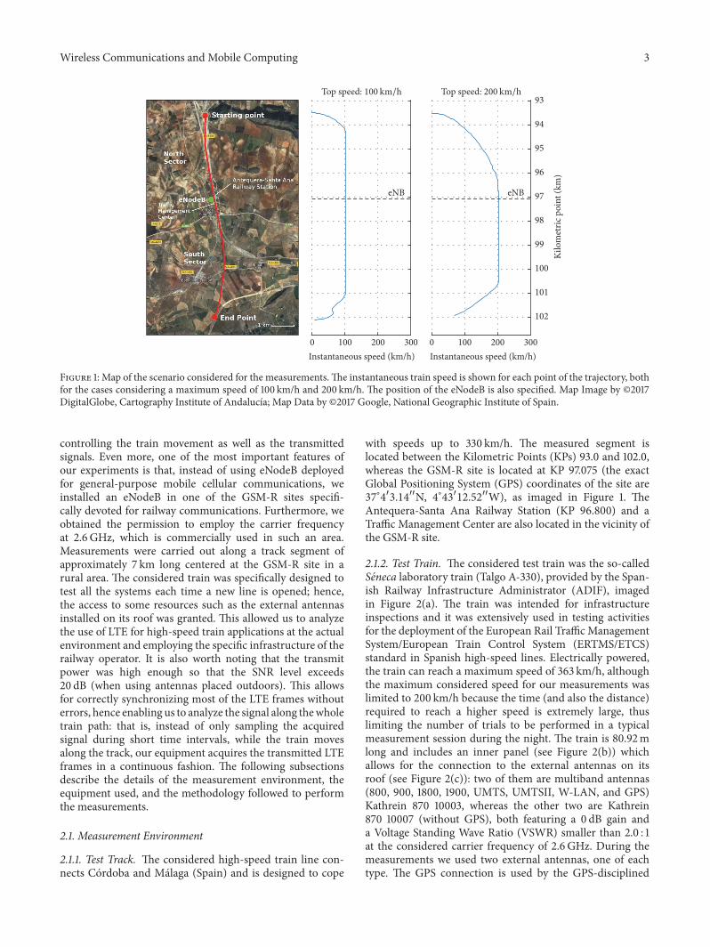
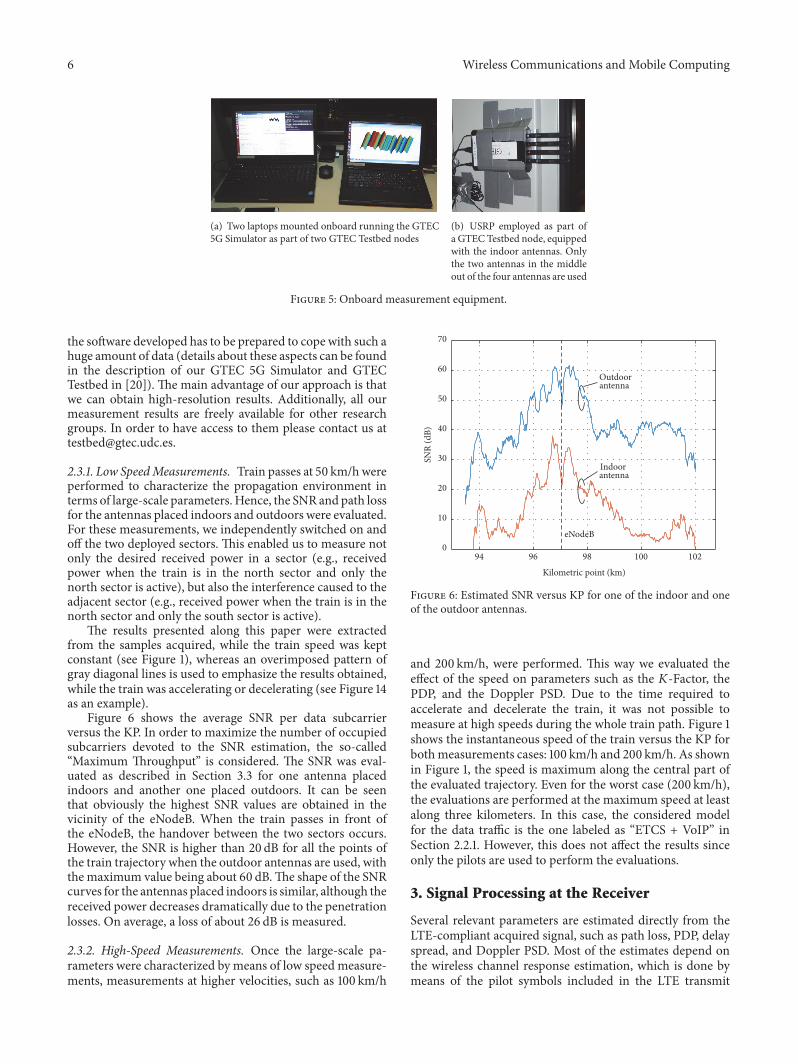
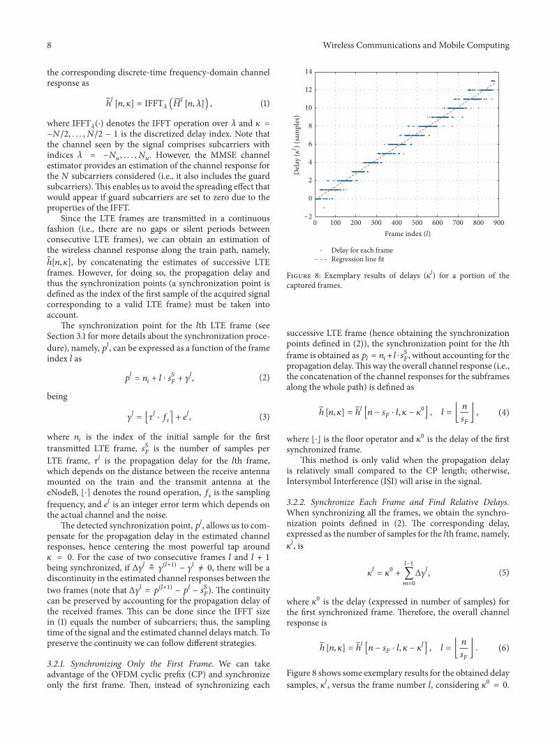
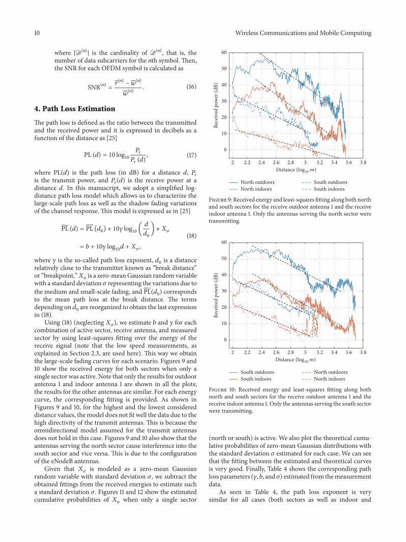
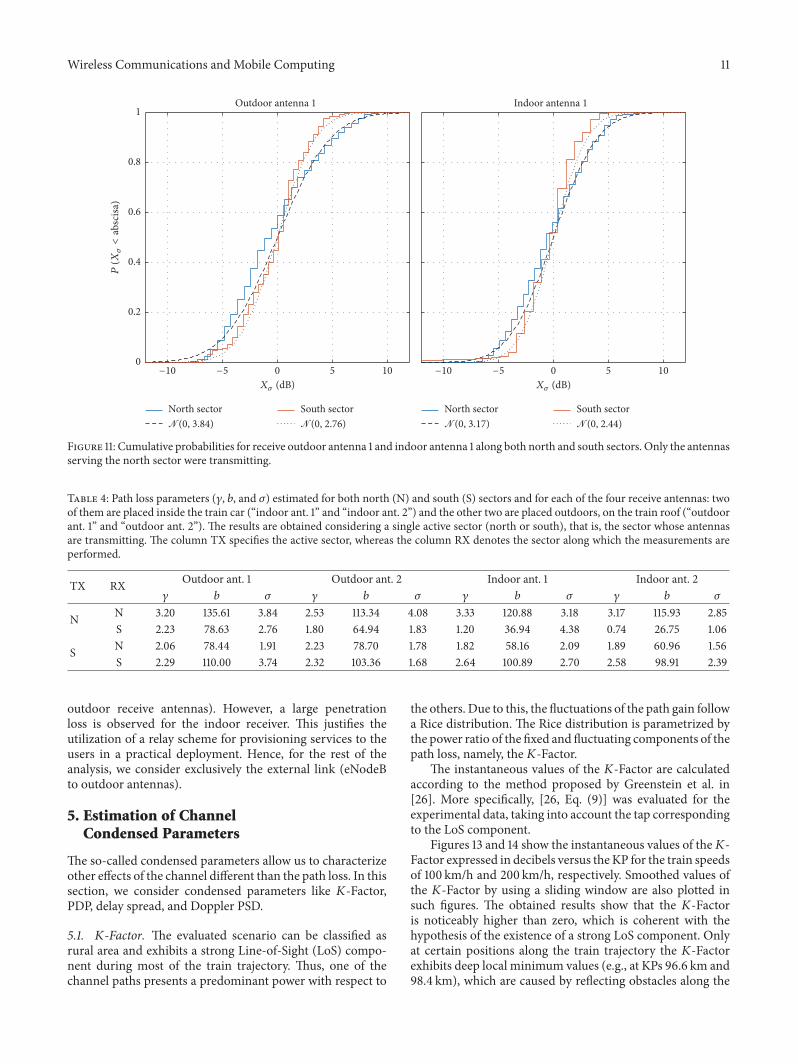
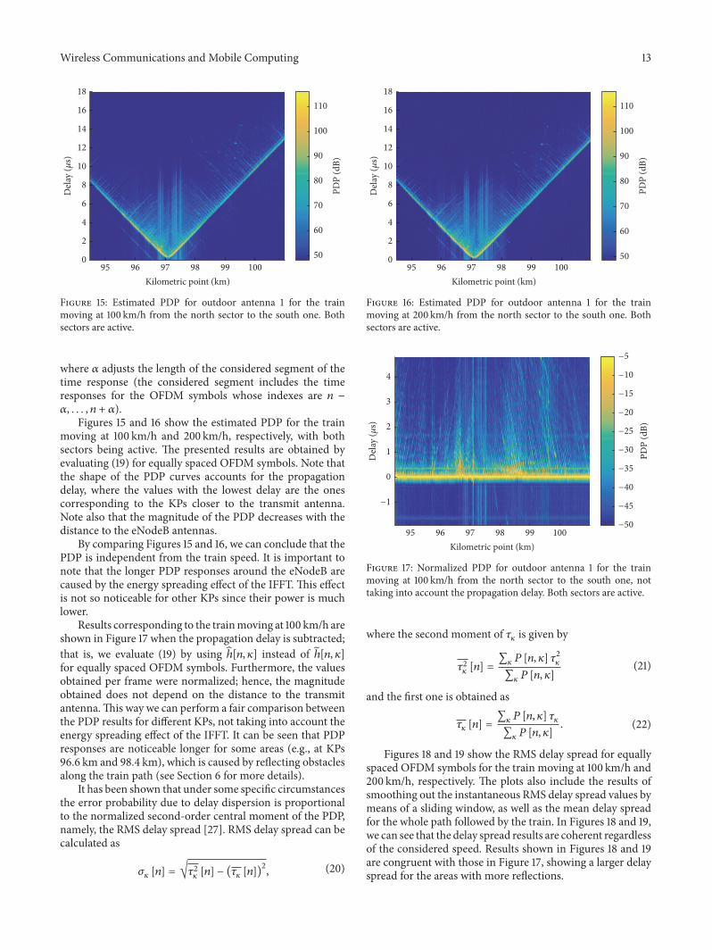
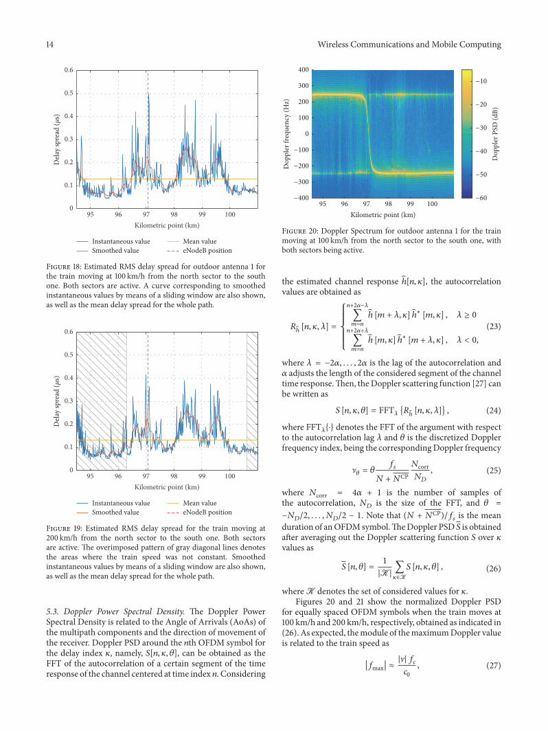
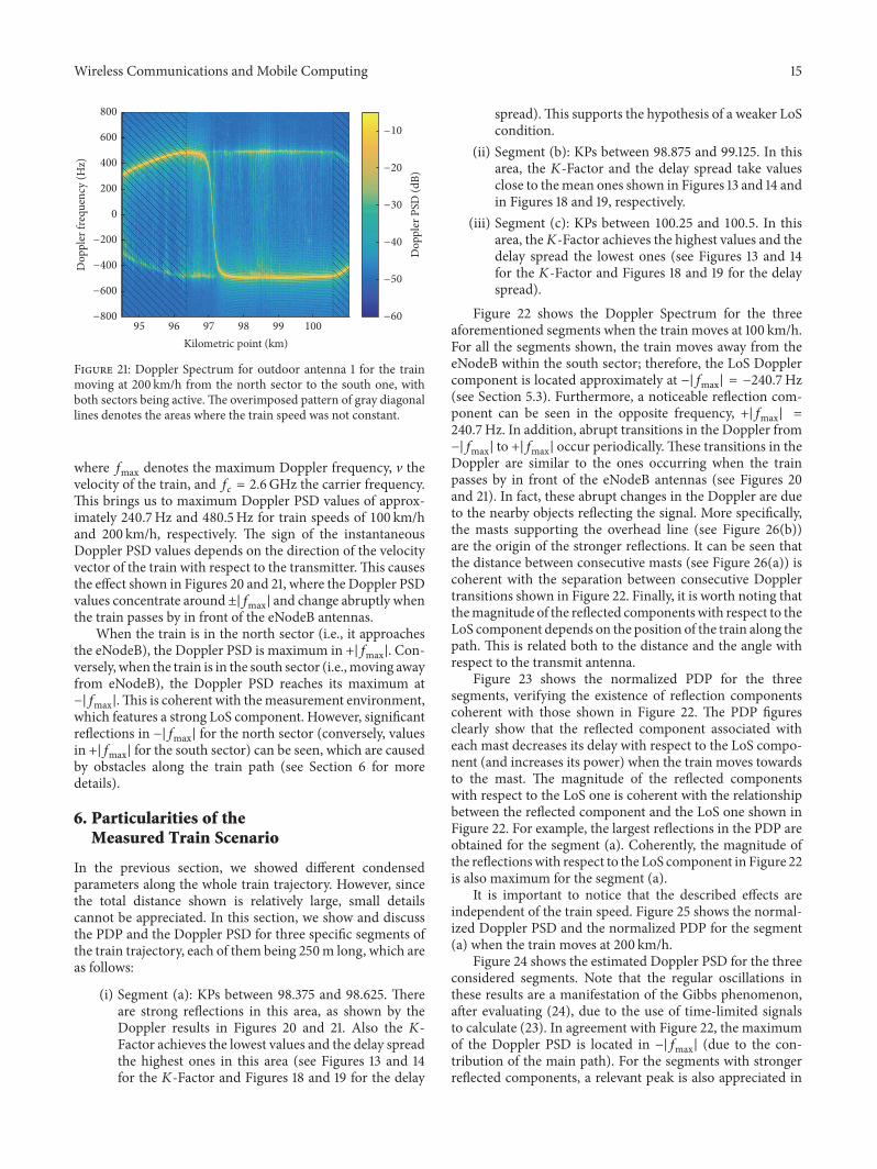
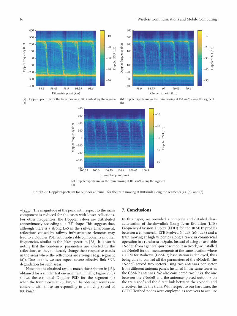
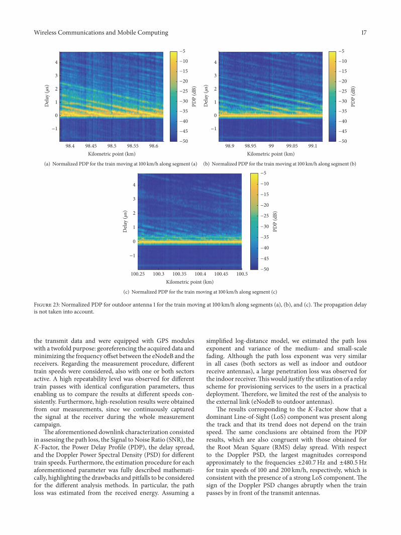
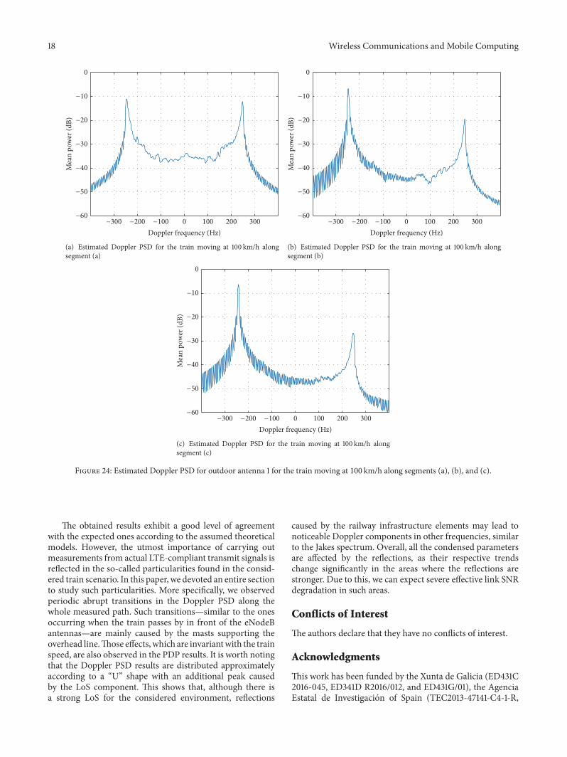
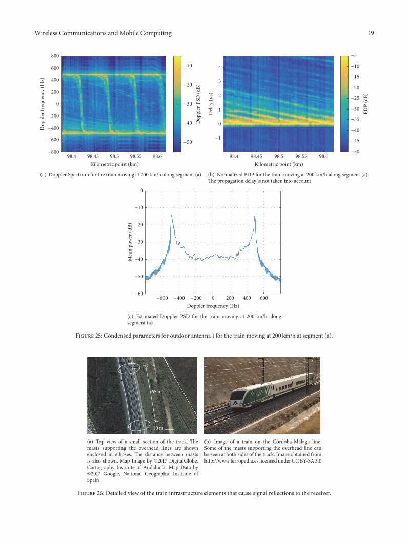