Embed Size (px)
Citation preview
0
POLITECNICO DI MILANO
Scuola di Ingegneria Civile, Ambientale e Territoriale
Corso di Laurea Magistrale in Ingegneria Civile
Experimental Characterization of Erosion in Abrasive Jet Impingement Tests
Relatore: Prof. Ing. Stefano Malavasi
Correlatori: Dott. Ing. Gianandrea Vittorio Messa
Dott. Ing. Marco Negri
Tesi di laurea Magistrale di:
Luigi Piani 853400
Anno accademico 2016/2017

0
Abstract
Flows carrying various amounts of solids, like sand particles, can be found in many
engineering fields, such as the oil and gas industry. These particles hit the solid walls,
thereby they gradually remove the material leading to damages to the plants and devices.
This phenomenon is called impact erosion. From a theoretical point of view, the impact
erosion is studied making reference to the ideal condition of a single impact between a
particle and a surface. This condition is usually approached experimentally by considering
jets of air and solid particles hitting a specimen for a certain time. The present work aims at
characterizing the impact erosion characteristics of materials by analogous tests with water
as carrying fluid (slurry jets). The tests are performed for different impinging conditions,
impact particles and specimens of several target materials like aluminum, different types of
steels and GRE (Glass Reinforced Epoxy), whose behavior under impact erosion has not
been deeply investigated so far. The campaign allowed assessing how the impact erosion
produced by slurry jets is affected by the most significant parameters. Afterwards, the
experimental analysis is extended from the specimen to a real-case geometry, which is a
choke valve installed in a slurry flow loop.
0
Summary
Summary ................................................................................................................... 0
1 Introduction ........................................................................................................ 7
1.1 Engineering relevance of the impact erosion issue .................................................................... 7
1.2 Erosion mechanism and related variables .................................................................................. 7
1.3 Apparatus for erosion characterization of materials ............................................................... 10
1.4 Functional dependence of the integral erosion ratio in abrasive jet impingement tests. ... 11
1.5 Tests in air ...................................................................................................................................... 12
1.6 Tests in water................................................................................................................................. 16
1.7 Single-particle erosion models .................................................................................................... 19
1.8 Aim of the work ............................................................................................................................. 20
2 Experimental set up ............................................................................................ 21
2.1 Description of the set up .............................................................................................................. 21
2.2 Methodology .................................................................................................................................. 27
2.3 Evaluation of uncertainties ......................................................................................................... 31
2.4 Materials .......................................................................................................................................... 44
2.4.1 Specimen Materials ................................................................................................................. 44
2.4.2 Abrasive Materials ................................................................................................................... 48
3. Results ................................................................................................................ 51
3.1 Tests on Aluminium ..................................................................................................................... 51
3.1.1 Analysis of the effect of the jet velocity and inclination ...................................................... 51
3.1.2 Analysis of the effect of concentration ............................................................................... 55
3.1.3 Analysis of the effect of abrasive granulometry ................................................................ 57
3.2 Tests on Aisi 410, Aisi 4130 and Inconel ................................................................................... 59
3.2.1 Analysis of the effect of the jet velocity .............................................................................. 59
3.2.2 Analysis of the effect of the jet inclination ........................................................................ 60
3.3 Test on GRE-Glass Reinforced Epoxy ........................................................................................ 64
3.3.1 Analysis of the effect of the jet inclination ........................................................................ 64
3.3.2 Analysis of the effect of the jet velocity .............................................................................. 66
4. Discussion of the results .................................................................................... 68
5. Application: erosion test on a valve .................................................................... 76
6. Conclusions ....................................................................................................... 83
Appendix .................................................................................................................. 85
A.1 Reliability of the pressure-flowrate curve ................................................................................. 86
A.2 Calibration of the 10mm nozzle .................................................................................................. 89
A.3 Calibration of the 8mm nozzle .................................................................................................... 92

1
A.4 Comparison between different flowmeters ............................................................................... 94
Appendix B ................................................................................................................................................ 95
References ............................................................................................................... 98
2
Index of the figures
Fig. 1 Single-particle condition: up refers to the impact velocity and θp to the impact angle. ............ 8
Fig. 2 Above, erosion procedure in ductile material (a) before the impact, (b) crater formation and
piling material at one side of the crater, (c) material separation. Below, expected erosion in brittle
material: (a) growth of the cone crack and median cracks, (b) closure of median and creation of
lateral cracks, (c) eroded crater formed (Parsi et al., 2014) ............................................................... 9
Fig. 3 Abrasive jet impingement with air: Vjet and θ can be considered equal to up and θp (Messa et
al., 2017) .............................................................................................................................................. 9
Fig. 4 Abrasive jet impingement with liquid: Vjet and θ cannot be considered equal to up and θp (Messa
et al., 2017) ........................................................................................................................................ 10
Fig. 5 different testing setups: (a) Slurry Pot Tester, Jha et al. (2010); (b) Direct impact test, Okita
et al. (2012), (c) Centrifugal accelerator, Kleis and Kulu (2008) ..................................................... 11
Fig. 6 comparison between eroded shapes: (a) U shape due to air test; W shape due to water test.
Mansouri et al. (2015) ....................................................................................................................... 12
Fig. 7 Dependence of ER on the impact velocity (θ=90°): a – 0.8% C with various fractions of sand;
b – 1 – hardmetal WC-6Co with corundum, 2- 0.8% steel with glass grit; Kleis and Kulu (2008) .. 13
Fig. 8 Dependence on impact angle θ at v=120 m/s, the diameter of particles 0.4-0.6 mm: a 0.2% C
steel – 1: with glass grit, 2: with corundum, 3: quartz sand, 4: 0.8% C steel with quartz sand; b 0.2%
steel – 1: with sharp-edged particles of cast iron, 2: with cast iron pellets; Kleis and Kulu (2008) 14
Fig. 9 wear curves of brittle materials: a -wear of enamel in quartz sand, d=0.16-0.3 mm, v=26 m/s;
1 with priming enamel, 2 enamel R193; b – sintered corundum worn with quartz sand, v=130 m/s; 1
d=1.0mm, 2 d=0.1mm, 3 d=0.01 mm; Kleis and Kulu (2008). ......................................................... 14
Fig. 10 Erosion dependence on particle size: the curves referrers to different impact velocities, Kleis
and Kulu (2008) ................................................................................................................................. 15
Fig. 11 Velocity influence on ERjet, Nguyen et al. (2014 .................................................................. 17
Fig. 12 Viscosity effect: a) effect of impact angle θ on the ERjet; b) effect of sand size on ERjet,
Mansouri et al. (2014) ....................................................................................................................... 17
Fig. 13 viscosity dependence for different particle size, Okita et al. (2012) ..................................... 18
Fig. 14 Influence of testing time, Nguyen et al. (2014). ..................................................................... 18
Fig. 15 Plastic deformation and cutting action contribution, Oka et al. (2005) ............................... 19
Fig. 16 Lower Tank and components ................................................................................................. 21
Fig. 17 Hydraulic System and components ........................................................................................ 22
Fig. 18 The two nozzles used and their diameter ............................................................................... 23
Fig. 19 Etanorm pump (KSB,2015) ................................................................................................... 24
Fig. 20 Detail of the eroded pump: 3 holes on the volute casing. ..................................................... 24
Fig. 21 Entrance of the water and impeller ....................................................................................... 25
Fig. 22 Impeller and eroded casing ................................................................................................... 25
Fig. 23 Detail of the volute casing ..................................................................................................... 25

3
Fig. 24 Control devices and instrumentation of the system ............................................................... 27
Fig. 25 Testing camera and its components ...................................................................................... 27
Fig. 26 Different inclination configuration ........................................................................................ 28
Fig. 27 60° configuration: the support is turned ............................................................................... 29
Fig. 28 Exit of the flux from the upper tank: place for concentration sampling ............................... 30
Fig. 29 Temperature reading ............................................................................................................. 31
Fig. 30 Concentration values during a test........................................................................................ 34
Fig. 31 First configuration in the filling set up: the tank is filled till the submersion of the nozzle .. 37
Fig. 32 First configuration in the sampling set up: the pipes are moved .......................................... 38
Fig. 33 Second configuration in the filling set up: all the pipes are fixed ......................................... 38
Fig. 34 Second configuration in the sampling set up same as the filling one: no pipes are moved .. 39
Fig. 35 Comparison between different sampling position in the first configuration and with the test
values ................................................................................................................................................. 40
Fig. 36 Comparison between different sampling position in the second configuration and with the test
values ................................................................................................................................................. 41
Fig. 37 Comparison between dried and mixture-based sampling ..................................................... 42
Fig. 38 Balance used for specimen weighing (Lab. Diagnostica e Analisi sui Materiali del Costruito
– DICA, Politecnico di Milano) ......................................................................................................... 43
Fig. 39 Large sand grading curve: the dashed lines refer to the maximum and minimum percentage
of particles for the diameters considered ........................................................................................... 49
Fig. 40 Medium sand grading curve: the dashed lines refer to the maximum and minimum percentage
of particles for the diameters considered ........................................................................................... 49
Fig. 41 Thin Sand grading curve: the dashed lines refer to the maximum and minimum percentage of
particles for the diameters considered ............................................................................................... 49
Fig. 42 Erosion effect, from right to left: 90°,60, 30° and 15°. Test duration 30 minutes ................ 51
Fig. 43 ER at 90° vs time duration of the test .................................................................................... 52
Fig. 44 ER values depending on the angle and duration under a jet velocity of 25 m/s ................... 52
Fig. 45 Normalized values of angle function for ER for 25m/s jet. ................................................... 53
Fig. 46 ER values depending on the angle with a jet velocity of 25 m/s ............................................ 53
Fig. 47 Normalized values of angle function for ER with 25 m/s jet velocity .................................... 54
Fig. 48 Profilometer result for a 30 minutes test with large sand at 90° and 27 m/s jet velocity ..... 54
Fig. 49 Profilometer result for a 15 minutes test with large sand at 30° and 25 m/s jet velocity. The
arrow points the direction of the flow ................................................................................................ 55
Fig. 50 ER values depending on the angle for the 0.3% concentration ............................................ 56
Fig. 51 ER values depending on the angle for the 1% configuration ................................................ 56

4
Fig. 52 Comparison between the ER angle function for 5 minutes’ tests with different concentration
of corundum ....................................................................................................................................... 57
Fig. 53 Normalized values of angle function for ER for both the configurations ............................. 57
Fig. 54 Comparison of ER with different sand size ........................................................................... 58
Fig. 55 Eroded specimens: Inconel under 25 and 30 m/s on the left; AISI 410 under 25 and 30 m/s on
the right .............................................................................................................................................. 59
Fig. 56 ER for all the steels under different jet velocities.................................................................. 60
Fig. 57 Eroded specimens of Aisi 410: from left to right 15° to 90° inclination. Reference graduation
in mm. For the inclined tests the jet impacts the specimens in the lower part .................................. 60
Fig. 58 ER values depending on the angle ......................................................................................... 61
Fig. 59 Erosion Effect on AISI 410: from left to right impacted by large sand, medium and thin .... 62
Fig. 60 Erosion Effect on AISI 4130: from left to right impacted by large sand, medium and thin .. 62
Fig. 61 Erosion Effect on AISI 410: from left to right impacted by large sand, medium .................. 62
Fig. 62 Comparison between ER for different sand used .................................................................. 63
Fig. 63 Erosion effect, from right to left: 5, 15 and 30 minutes duration at 15° inclination ............. 64
Fig. 64 Erosion effect, from right to left: 5, 15 and 30 minutes duration at 30° inclination. ............ 64
Fig. 65 Erosion effect, from right to left: 5, 15 and 30 minutes duration at 90° inclination ............. 65
Fig. 66 ER values at 33 m/s depending on the angle and duration ................................................... 65
Fig. 67 ER at 21 m/s depending on the angle and duration .............................................................. 66
Fig. 68 ER dependence on velocity along time .................................................................................. 66
Fig. 69 Repeatability of the test on the GRE...................................................................................... 67
Fig. 70 ER dependence on velocity for different target material and same impacting sand ............. 69
Fig. 71 Aluminum dependence on velocity for different impacting sand ........................................... 70
Fig. 72 Comparison between scaled ER with literature’s values (Messa et al, 2017) ...................... 71
Fig. 73 GRE dependence on velocity for different testing times hit by thin sand 1% ........................ 72
Fig. 74 ER dependence on Brinnel hardness of target materials ...................................................... 72
Fig. 75 Comparison of all target materials: Aluminum is tested with large sand, Aisi 410 with
medium sand and GRE with thin sand ............................................................................................... 73
Fig. 76 Comparison of the angle dependence of Aluminum: a 5 minutes’ test with corundum 1% and
a 30 minutes’ test with Large sand 1% .............................................................................................. 73
Fig. 77 ERv comparison for different target materials: Aluminum is tested with large sand, Aisi 410
with medium sand and GRE with thin sand ....................................................................................... 74
Fig. 78 ER dependence on abrasive material size (sand) for different targets ................................. 75
Fig. 79 Erosion Loop system at G.Fantoli Laboratory ...................................................................... 76
Fig. 80 Choke Valve installed on the loop system. ............................................................................ 77
Fig. 81 Internal details of the Choke valve ........................................................................................ 78
5
Fig. 82 Numeration of the cage ......................................................................................................... 78
Fig. 83 Cage erosion during the tests: view from hole 1 ................................................................... 79
Fig. 84 Cage erosion during the tests: view from hole 3 ................................................................... 79
Fig. 85 Cage erosion during the tests: view from hole 5 ................................................................... 79
Fig. 86 Cage erosion during the tests: view from hole 7 ................................................................... 79
Fig. 87 Details of the bigger holes (2, 4, 6, 8) before and after the test ............................................ 80
Fig. 88 Details of the smaller holes (1, 3, 5, 7) before and after the test .......................................... 81
Fig. 89 Time evolution of the mass loss of the valve cage: experimental data and fitting line. The scale
has a precision of 0.1 g. ..................................................................................................................... 81
Fig. 90 Experimentally determined flow coefficient versus pipe Reynolds number before and after the
test ...................................................................................................................................................... 82
Fig. 91 Nozzle Q-H curve from the factory ........................................................................................ 86
Fig. 92 Detail of the pipes between nozzle and pressure gauge ........................................................ 87
Fig. 93 Comparison of a used nozzle (left) and a new one (right) .................................................... 88
Fig. 94 Comparison between curves by submerged and not submerged nozzle ................................ 89
Fig. 95 Comparison of Q-H curves for different time use of the nozzle ............................................ 90
Fig. 96 Variation with time of the parabola coefficients ................................................................... 90
Fig. 97 Variation with Kg of sand of parabola coefficients............................................................... 91
Fig. 98 Nozzle diameter variation with Kg of sand ........................................................................... 92
Fig. 99 Comparison of the Q-H curve of the plant for the two pumps .............................................. 93
Fig. 100 Comparison of the Q_H curve of the plant with the 8 mm diameter nozzle for different time
use ...................................................................................................................................................... 93
Fig. 101 System Q-H curve by different devices ................................................................................ 94
Fig. 102 System Q-H curve measured by Ultrasonic flowmeter, in case of water and slurry flow ... 94
Fig. 103 Standard deviation of flowrate in case of water and slurry flow. ....................................... 95
6
Index of the tables
Tab. 1 System Feature ........................................................................................................................ 22
Tab. 2 Amount of particles and duration before pump’s breakdown ................................................ 24
Tab. 3 Tolerance of the measurement devices ................................................................................... 32
Tab. 4 tolerance, resolution and total uncertainty on the main measured parameters ..................... 33
Tab. 5 percentile for a two-tail t student distribution ........................................................................ 35
Tab. 6 30 minutes’ test with sand with two flasks: each line refers to concentration samples at a
different increasing time .................................................................................................................... 35
Tab. 7 5 minutes’ test with corundum with one flask: each line refers to concentration samples at a
different increasing time .................................................................................................................... 36
Tab. 8 10 minutes’ test with sand with one flask: each line refers to concentration samples at a
different increasing time .................................................................................................................... 36
Tab. 9 Concentration values during a regular test: test values sampled only in the lower tank....... 40
Tab. 10 values for mixture-based and static concentration ............................................................... 42
Tab. 11 Properties (http://www.anodallgroup.com/images/files/LEGA_6082.pdf) .......................... 45
Tab. 12 Chemical composition (http://www.anodallgroup.com/images/files/LEGA_6082.pdf) ....... 45
Tab. 13 Properties (http://www.centroinox.it/sites/default/files/pubblicazioni/245A.pdf) ................ 45
Tab. 14 Chemical composition given by the producer, Eure Inox S.r.l ............................................. 46
Tab. 15 Properties (https://www.azom.com/article.aspx?ArticleID=6742) ...................................... 46
Tab. 16 Chemical composition (https://www.azom.com/article.aspx?ArticleID=6742) ................... 46
Tab. 17 Properties, ASTM international B637 12 ............................................................................. 47
Tab. 18 Chemical composition, ASTM international B637 12 .......................................................... 47
Tab. 19 Properties given by the producer, Sabbie Sataf ................................................................... 48
Tab. 20 Chemical composition given by the producer, Sabbie Sataf ................................................ 48
Tab. 21 Mean diameter given by the producer, Sabbie Sataf ............................................................ 50
Tab. 22 Properties (http://www.techmasrl.com/p46/corindone/) ...................................................... 50
Tab. 23 Chemical composition (http://www.techmasrl.com/p46/corindone/) ................................... 50
Tab. 24 Coefficient of variation using m=2.41 and optimum n value ............................................... 69
Tab. 25 Losses between nozzle and pressure guage. Each line refers to three velocity chosen: 1.8 l/s,
2 l/s and 2.2 l/s ................................................................................................................................... 87
Tab. 26 Head Loss and flowrate estimation ...................................................................................... 88
Tab. 27 Values of the parabola coefficients ....................................................................................... 90
Tab. 28 Values of the parabola coefficients ....................................................................................... 91
Tab. 29 report of all the tests and main parameters’ values ............................................................. 95

1.1 Engineering relevance of the impact erosion issue
7
1 Introduction
1.1 Engineering relevance of the impact erosion issue
Fluids with solid particles are commonly encountered in the Oil & Gas industry. For example, the oil
extraction processes involve a multiphase mixture of oil, gases, water and sand.
The solid particles hit the plant component such as pipes, elbows, valves etc. and they gradually
remove material. This phenomenon is called impact erosion. In this way, the components are damaged
and, in most cases, they must be repaired or even replaced.
In order to limit the damage by erosion, wear resistant materials or surface coatings are used. Actually,
the problem of erosion cannot be completely avoided, nevertheless being capable in predicting the
occurrence and the extent of erosion is fundamental to limit its consequences by improving the design
and the management of the plants.
A work by Wood and Wheeler (1998) mentions an earlier report by BP, which, based on the analysis
of a sample of control valves used in the oil & gas industry subjected to impact erosion, came to the
following conclusions. About 35% of the devices were out of service only after two years and, in
some cases, they broke down within a few hours, despite being supposed to last at least 18 months.
The cost for substituting this kind of valves is very high, up to about £300000 each. Besides, the
related problems (and therefore the costs) of unpredicted breakage and loss of production should be
considered.
It is necessary to monitor very carefully all the devices that are subjected to impact erosion and
identify their most vulnerable components.
During the last years, many researchers tried to develop methods and models for a fast quantitative
prediction of erosion, paying more attention to the hydraulic singularities which are most affected by
the phenomenon.
1.2 Erosion mechanism and related variables
The impact erosion is the removal of material caused by impinging solid particles transported by a
fluid, which can be either a single-phase one (e.g. water, air, oil) or a multiphase mixture.
Erosion is quantified by several parameters, such as:
• Erosion Ratio 𝐸𝑅 [𝑀
𝑀] =
𝑊2−𝑊1
𝑀𝑠 where 𝑊 is the mass of a certain object, the subscripts 1 and
2 stand for initial and final time, respectively. 𝑀𝑠 is the solid (subscript “s”) mass impacting
the object, e.g. sand;
• 𝐸𝑅𝑣 [𝑉
𝑀] =
𝑉2−𝑉1
𝑀𝑠 refers to the removed volume. V stands for the volume and the subscripts
have the same meaning of those for ER;
• Erosion Rate 𝐸 [𝑀
𝑇] =
𝑊2−𝑊1
𝑇 where T is the time interval considered;

1.2 Erosion mechanism and related variables
8
• Penetration Rate 𝑃𝑅 [𝐿
𝑇] =
ℎ2𝑖−ℎ1𝑖
𝑇 where ℎ𝑖 is the local thickness of an object subjected to
erosion.
The previous parameters, expect for PR, refer to an integral approach: they consider the whole object
at two different times. On the other hand, PR is based on distributed approach, being defined on each
point of the surface of the considered object. Nevertheless, local formulations of ER, ERv and E exist
as well.
Usually, all the functional dependences are studied referring to a single-particle condition in which a
single impact of one particle is considered, Fig. 1. In this case, the ERsp is the removed mass divided
by the mass of the particle.
Fig. 1 Single-particle condition: up refers to the impact velocity and θp to the impact angle.
The single-particle condition is very relevant. For instance, all the numerical models for the prediction
of the erosion describe the solid phase with the Lagrangian approach, i.e. following each single
particle’s motion, and they superimpose the effect on the single-particle condition using an erosion
model. Moreover, this condition is the base of most of the studies concerning the wear from the point
of view of the solid mechanics (fracture and damage mechanics).
The erosion for this configuration mainly depends on:
1. Modulus of velocity at the impact stage, up.
2. Impact angle, θp.
3. Some mechanic features of the target material, such as the hardness.
4. Some geometric and mechanic features of the particle such as the dimension, the shape, the
hardness and the density.
The basic mechanisms of the erosion phenomenon are reported in Fig. 2: the deformation wear is
generally related to ductile target materials while the cutting wear refers to brittle ones.
The functional relationship for the single-particle condition can be expressed as follow:
𝐸𝑅𝑠𝑝 = 𝑓(𝑢𝑝, 𝜃𝑝, 𝑡𝑎𝑟𝑔𝑒𝑡, 𝑝𝑎𝑟𝑡𝑖𝑐𝑙𝑒)

1.2 Erosion mechanism and related variables
9
Fig. 2 Above, erosion procedure in ductile material (a) before the impact, (b) crater formation and piling material at one side of the
crater, (c) material separation. Below, expected erosion in brittle material: (a) growth of the cone crack and median cracks, (b)
closure of median and creation of lateral cracks, (c) eroded crater formed (Parsi et al., 2014)
For the single-particle condition, the duration of test and the concentration of solids play no role since
only one impact is considered. That’s why this is an ideal case, in reality hundreds and thousands of
particles are involved in the process. The large number of particles affects the fluid dynamics of the
fluid-particle system, thus the trajectories of the particles and therefore the number, the angle and the
velocity of the impacts.
Reproducing a single-particle condition experimentally is very hard since the quantities (mass loss)
to be measured are very small. The closest test to this condition is called “abrasive jet impingement”,
in which a fluid jet containing solid particles impacts against a specimen, Fig. 3 for an air jet.
Fig. 3 Abrasive jet impingement with air: Vjet and θ can be considered equal to up and θp (Messa et al., 2017)
Fig. 4 refers to liquid jet. The differences between the two cases will be deeply investigated in the
following pages.

1.2 Erosion mechanism and related variables
10
Fig. 4 Abrasive jet impingement with liquid: Vjet and θ cannot be considered equal to up and θp (Messa et al., 2017)
Global variables (referred to the jet-specimen system) and local ones (referred to a single particle)
are different: considering a jet implies that also the type of fluid, the interaction between particles,
the testing time and the change of geometry of the specimen come into play. So, the erosion process
in an abrasive jet impingement test depends also on the concentration of impact particles, the time
and the carrying fluid properties.
The functional relationship for the abrasive jet impingement condition can be expressed as follow:
𝐸𝑅𝑗𝑒𝑡 = 𝑓(𝑉𝑗𝑒𝑡, 𝜃, 𝑓𝑙𝑢𝑖𝑑, 𝑡𝑎𝑟𝑔𝑒𝑡, 𝑝𝑎𝑟𝑡𝑖𝑐𝑙𝑒, 𝑐𝑜𝑛𝑐𝑒𝑛𝑡𝑟𝑎𝑡𝑖𝑜𝑛, 𝑡𝑖𝑚𝑒)
The goal of abrasive jet impingement tests can be both the characterization of the functional
relationship and the comparison of different materials as well as the evaluation of the effectiveness
of coatings.
1.3 Apparatus for erosion characterization of materials
The characterization of the behaviour of material under erosion conditions can be achieved with
different experimental setups. Air flows are mainly used since they are more similar to the single-
particle condition: impact velocity and angle can be approximated with the jet-specimen system
because the fluid has not a strong influence on the particles. Nevertheless, the interaction between
particles and the change of geometry must be considered as well. Abrasive jet impingements are
differently arranged in the various apparatus. For instance, in the slurry pot tester is based on a
centrifugal system which makes the specimen rotate at different velocities. The specimens are placed
in a cabine filled with solid-liquid mixture (Fig. 5a). Conversely, in the direct impact test setup the
abrasive mixture is pumped through the nozzle and hits the specimen. This kind of setup is generally
composed by a pump, a tank, a reservoir tank and a testing cabine (Fig. 5b).
1.3 Apparatus for erosion characterization of materials
11
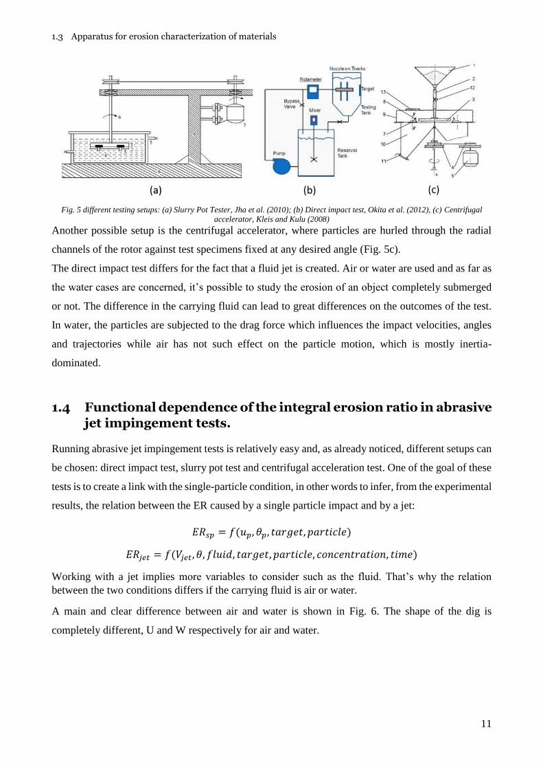
Fig. 5 different testing setups: (a) Slurry Pot Tester, Jha et al. (2010); (b) Direct impact test, Okita et al. (2012), (c) Centrifugal
accelerator, Kleis and Kulu (2008)
Another possible setup is the centrifugal accelerator, where particles are hurled through the radial
channels of the rotor against test specimens fixed at any desired angle (Fig. 5c).
The direct impact test differs for the fact that a fluid jet is created. Air or water are used and as far as
the water cases are concerned, it’s possible to study the erosion of an object completely submerged
or not. The difference in the carrying fluid can lead to great differences on the outcomes of the test.
In water, the particles are subjected to the drag force which influences the impact velocities, angles
and trajectories while air has not such effect on the particle motion, which is mostly inertia-
dominated.
1.4 Functional dependence of the integral erosion ratio in abrasive
jet impingement tests.
Running abrasive jet impingement tests is relatively easy and, as already noticed, different setups can
be chosen: direct impact test, slurry pot test and centrifugal acceleration test. One of the goal of these
tests is to create a link with the single-particle condition, in other words to infer, from the experimental
results, the relation between the ER caused by a single particle impact and by a jet:
𝐸𝑅𝑠𝑝 = 𝑓(𝑢𝑝, 𝜃𝑝, 𝑡𝑎𝑟𝑔𝑒𝑡, 𝑝𝑎𝑟𝑡𝑖𝑐𝑙𝑒)
𝐸𝑅𝑗𝑒𝑡 = 𝑓(𝑉𝑗𝑒𝑡, 𝜃, 𝑓𝑙𝑢𝑖𝑑, 𝑡𝑎𝑟𝑔𝑒𝑡, 𝑝𝑎𝑟𝑡𝑖𝑐𝑙𝑒, 𝑐𝑜𝑛𝑐𝑒𝑛𝑡𝑟𝑎𝑡𝑖𝑜𝑛, 𝑡𝑖𝑚𝑒)
Working with a jet implies more variables to consider such as the fluid. That’s why the relation
between the two conditions differs if the carrying fluid is air or water.
A main and clear difference between air and water is shown in Fig. 6. The shape of the dig is
completely different, U and W respectively for air and water.

1.4 Functional dependence of the integral erosion ratio in abrasive jet impinging tests
12
Fig. 6 comparison between eroded shapes: (a) U shape due to air test; W shape due to water test. Mansouri et al. (2015)
1.5 Tests in air
The characterization of erosion by impact has been studied for many years. One of the most complete
works is done by Kleis and Kulu (2008) who collected a lot of different results from many researchers
in the last 30 years of the 1900.
All the work by Kleis and Kulu (2008) focuses on the erosion in air. Using air as a fluid makes
possible to approximate the impact velocities of the jet with that of the single particle, as well as the
impact angle: this is due to the particle’s high inertia which makes the influence of the fluid almost
negligible. So, the functional relationship is the following:
𝐸𝑅𝑗𝑒𝑡 = 𝑓(𝑉𝑗𝑒𝑡, 𝜃, 𝑡𝑎𝑟𝑔𝑒𝑡, 𝑝𝑎𝑟𝑡𝑖𝑐𝑙𝑒, 𝑐𝑜𝑛𝑐𝑒𝑛𝑡𝑟𝑎𝑡𝑖𝑜𝑛, 𝑡𝑖𝑚𝑒)
Moreover, Kleis and Kulu (2008) used a centrifugal vacuum collector tester in order to prevent any
possible effect due to air. Nowadays, is difficult to find in literature studies on erosion by a direct
impact test in water. The impact velocity (𝑉𝑗𝑒𝑡), is the most affecting parameter. Generally, the erosion
ratio can be expressed by:
𝐸𝑅𝑣 [𝑚𝑚3
𝑘𝑔] = 𝑎 ∙ 𝑉𝑗𝑒𝑡
𝑚
Where the coefficient 𝑎 depends on the target material, the impact angle and the proprieties of the
abrasive material; while the exponent 𝑚 depends mainly on the target material. According to Kleis
and Kulu (2008), m varies from 1.4 for steel to 4.6 for rubber.
Moreover, both a and m depend on the particles, as shown in Fig. 7. In fact, the value of ER for a
given 𝑉𝑗𝑒𝑡 changes with particles size and varies a lot with coarse grains, which are considered the
most defective ones. It’s also clear that up to a threshold of velocity, the inclination of the lines is
constant and very similar for different sizes. However, m shouldn’t be considered a constant since it
can vary because the abrasive particles can break up during the test.

1.5 Tests in air
13
Fig. 7 Dependence of ER on the impact velocity (θ=90°): a – 0.8% C with various fractions of sand;
b – 1 – hardmetal WC-6Co with corundum, 2- 0.8% steel with glass grit; Kleis and Kulu (2008)
Moreover, it was found that m is smaller for sharp edged particles in comparison with rounded ones.
However, typical values used for m vary from 1.6 to 2.6 (Parsi et al, 2014).
Another influencing parameter is the impact angle θ between the particles’ velocity vector and the
specimen. Parsi and co-workers remark the different behavior of brittle and ductile target material:
the first is eroded by a cracking mechanism and the latter follows a plastic behavior. Generally, 𝐸𝑅𝑗𝑒𝑡
for brittle materials grows with θ (Fig. 8) while for ductile materials there’s a maximum and then a
decrease (Fig. 9). The same effect is reported by Kleis and Kulu (2008), who observed a
monotonically increasing dependence on θ also for hardened steels.
As for the exponent m, the dependence on the impact angle is affected, above all, by the target material
and the particles’ shape. As shown in Fig. 8 and Fig. 9, the maximum of the wear rate is approximately
between 17° and 45° for soft steel and between 60° and 90° for hardened steel. In the cases of soft
steels, for a fixed velocity, Kleis and Kulu (2008) found that the sharper the particles are the smaller
the impact angle at which the maximum wear rate is reached and the rounder the particles are the
flatter the curve is.

1.5 Tests in air
14
Fig. 8 Dependence on impact angle θ at v=120 m/s, the diameter of particles 0.4-0.6 mm:
a 0.2% C steel – 1: with glass grit, 2: with corundum, 3: quartz sand, 4: 0.8% C steel with quartz sand;
b 0.2% steel – 1: with sharp-edged particles of cast iron, 2: with cast iron pellets; Kleis and Kulu (2008)
Fig. 9 wear curves of brittle materials: a -wear of enamel in quartz sand, d=0.16-0.3 mm, v=26 m/s; 1 with priming enamel, 2
enamel R193; b – sintered corundum worn with quartz sand, v=130 m/s; 1 d=1.0mm, 2 d=0.1mm, 3 d=0.01 mm; Kleis and Kulu
(2008).
The influence of particles size on the wear rate is probably the most demanding issue and it’s still far
to be well defined. In general, it seems that a larger particle leads to a bigger dig, but the impact
velocity (Fig. 10) and the impact angle affect the process.
Particle size is even more complicated in systems with the recirculation of the abrasive mixture. The
impact against the specimen can break the particle itself, leading to a variation in the ER with time.

1.5 Tests in air
15
Also in systems without recirculation, it might be that particles bounce more than once on the surface
leading to the modification of particle’s size.
The particle diameter, as well as its shape, can lead to different curves of 𝐸𝑅𝑗𝑒𝑡 against θ.
Fig. 10 Erosion dependence on particle size: the curves referrers to different impact velocities, Kleis and Kulu (2008)
As already noticed, Kleis and Kulu (2008) highlights that, when brittle particles are used, there exists
a threshold velocity above which the particle is fragmented, leading a decline in the wear rate.
Desale et al. (2009) found that the erosion ratio is proportional to particle size elevated by n, which
can vary between 0.3 and 2, depending on differences in the material properties, experimental
conditions, particle velocity and even and size distribution, since generally the dp,50 is used. In general,
smaller sand is thought to cause lower erosion ratios since it has smaller kinetic energy and impact
force. Nevertheless, particle density, shape and hardness affect erosion, even though larger sand in
general causes more erosion for similar condition.
Erosion due to small particles may also be affected by particle-particle interactions as the number of
particles increases as the size decreases (for the same mass of impacting particles).
These small particles are more influenced by the fluid turbulence, but this is a typical effect of systems
using water as carrier mean and, therefore, it will be discussed later.
Moreover, the ratio between target and impact material hardness has a correlation with the erosion
ratio, which rapidly increases with the increasing of the ratio of erodent to target hardness toward
unity (Shipway and Hutchings, 1996). Also Arabnejad et al. (2015) found that “the hardness effect is
remarkable when the hardness of a particle is less than the hardness of the target material and the
erosion ratio doesn’t increase significantly when the particle hardness is relatively higher than the
material hardness and the particle keeps its integrity during the impact”

1.6 Tests in water
16
The last important parameter is the particle concentration. Kleis and Kulu (2008) found that its effect
generally depends on:
• Impact velocity. The effect of particle concentration increases with velocity, the influence of
concentrations at v=115 m/s is 2.1 greater than at v=56 m/s;
• Impact angle. A certain increase of the effect was observed at greater impact angles;
• Crushing of abrasive particles. The effect of quartz was 1.4 times greater than that of cast iron
pellets with identical size
• Particle size. The effect of concentration was greater with smaller particles.
Basically, a screening effect is connected with concentration, meaning that the bouncing particles
interact with the incoming ones, leading to a decrease of the erosion ratio.
Another one important parameter is the testing time which must be considered not as a time itself but
as a change in the specimen geometry. This effect has been studied by Nguyen (2014) who found out
that ER decreases with the testing time and so the change on geometry affects the impact characteristic
(impact angle and velocity) and so the erosion mechanism.
Testing time affects also the mechanical properties of the particles since a fragmentation of the
particles might occur during the test.
Thus, the results obtained with an abrasive jet impingement system in air can be considered
representative of the single-particle condition if the testing time and the concentration are sufficiently
small.
1.6 Tests in water
Using water as carrying fluid leads to a more complicated characterization of the functional
relationship. In this case, the hypothesis of 𝑢𝑝 ≈ 𝑉𝑗𝑒𝑡 and 𝜃𝑝 ≈ 𝜃 is no more valid since now the liquid
affects the motion of the particle. The complete functional relationship must be considered.
𝐸𝑅𝑗𝑒𝑡 = 𝑓(𝑉𝑗𝑒𝑡, 𝜃, 𝑓𝑙𝑢𝑖𝑑, 𝑡𝑎𝑟𝑔𝑒𝑡, 𝑝𝑎𝑟𝑡𝑖𝑐𝑙𝑒, 𝑐𝑜𝑛𝑐𝑒𝑛𝑡𝑟𝑎𝑡𝑖𝑜𝑛, 𝑡𝑖𝑚𝑒)
Inferring a relation with the single-particle condition from water experiments is hard and it requires
CFD models: probably this is one of reasons of the scarcity of literature referring to water abrasive
jet impingement condition. This type of tests is usually done for determining the wear characteristics
of different materials or for validating CFD models.
Velocity and angle of the jet are still the most important parameters. Generally, 𝐸𝑅𝑗𝑒𝑡 increase with
velocity (Fig. 11) which, contrary to the air case, doesn’t reach very high values. Based on the studies
found in the literature review, the maximum jet velocity in water tests is about 30-40 m/s.

1.6 Tests in water
17
Fig. 11 Velocity influence on ERjet, Nguyen et al. (2014
Two interesting works by Mansouri et al. (2014) and Okita et al. (2012) considered carrier fluids with
different viscosity. According to Mansouri et al. (2014), the viscosity is effective only at lower angles
(Fig. 12a), probably due to the different fluid dynamic characteristics that rise near the specimen.
Fig. 12 Viscosity effect: a) effect of impact angle θ on the ERjet; b) effect of sand size on ERjet, Mansouri et al. (2014)
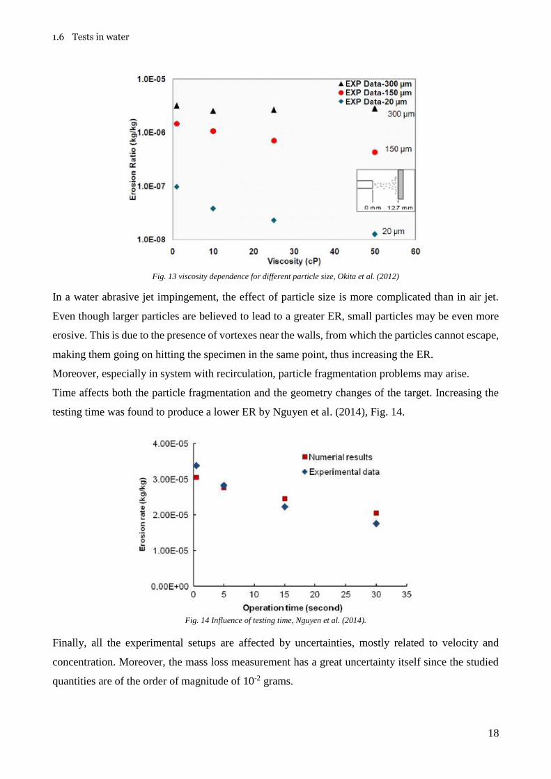
The dependence of viscosity is not affected by particle size according to Mansouri (Fig. 12b), whilst
opposite findings are observed by Okita, Fig. 13, according to whom the smaller the particle the
bigger the effect of the viscosity. The different results may be due to the different target material and
different velocity, 14 m/s and 10 m/s respectively.
1.6 Tests in water
18
Fig. 13 viscosity dependence for different particle size, Okita et al. (2012)
In a water abrasive jet impingement, the effect of particle size is more complicated than in air jet.
Even though larger particles are believed to lead to a greater ER, small particles may be even more
erosive. This is due to the presence of vortexes near the walls, from which the particles cannot escape,
making them going on hitting the specimen in the same point, thus increasing the ER.
Moreover, especially in system with recirculation, particle fragmentation problems may arise.
Time affects both the particle fragmentation and the geometry changes of the target. Increasing the
testing time was found to produce a lower ER by Nguyen et al. (2014), Fig. 14.
Fig. 14 Influence of testing time, Nguyen et al. (2014).
Finally, all the experimental setups are affected by uncertainties, mostly related to velocity and
concentration. Moreover, the mass loss measurement has a great uncertainty itself since the studied
quantities are of the order of magnitude of 10-2 grams.

1.7 Single particle erosion models
19
1.7 Single-particle erosion models
Single-particle erosion models are mathematical functions which aim at quantifying the functional
dependencies of the single-particle condition, based on the experimental data from abrasive jet
impingement test.
However, as can be easily understood from the previous paragraphs, a complete description of all the
parameters during a test is almost impossible. The difficulty of controlling all the parameters is
reflected in the many models of prediction of erosion that can be found in literature. Since
experimental result are intrinsically affected by errors, for instance in the concentration measurements
during a test, which is almost never explained in research papers, each model gives a different
prediction based on its own experimental data.
Nowadays, the most widely used erosion models are those developed by Oka and the Erosion-
Corrosion Research Center (E/CRC) at the University of Tulsa.
Oka developed its model considering that erosion is affected by impact velocity, angle, size and type
of particles and material hardness. In order to express the angle dependence, a function g(𝜗) is
introduced and represent the ratio between the erosion damage at arbitrary angles to that at normal
angle.
𝐸𝑅𝑣(𝜗) = 𝑔(𝜗)𝐸90
Where 𝐸𝑅𝑣 is the unit of material volume removed per mass of particles (mm3/kg).
g(𝜗) represents the combination of two trigonometric functions and the material hardness number Hv
(GPa),Fig. 15.
𝑔(𝜗) = (𝑠𝑖𝑛𝜗)𝑛1 ∙ (1 + 𝐻𝑣(1 − 𝑠𝑖𝑛𝜗))𝑛2
where 𝑛1 and 𝑛2 depend on the material hardness and other particle properties. Graphically, g(𝜗)
behaves as follows:
Fig. 15 Plastic deformation and cutting action contribution, Oka et al. (2005)

1.8 Aim of the work
20
Basically, Oka divides the angle dependence in two main contributions: first term is the repeated
plastic deformation (brittle behavior), and second term is the cutting action.
Concerning the erosion at normal angle, Oka and co-workers propose the following formula.
𝐸90 = 𝐾 ∙ (𝐻𝑣)𝑘1 ∙ (𝑢𝑝
𝑢′)𝑘2 ∙ (
𝐷𝑝
𝐷′)𝑘3
where k1, k2 and k3 are exponent factors, K denotes a particle property factor such as particle shape
and particle hardness. 𝐷𝑝 and 𝑢𝑝 are respectively the particle diameter and the impact velocity, whilst
D’ and u’ are normalization factors suggested by the authors. Besides, in their papers, Oka et al.
explains very well how all the parameters vary with the depending quantities.
The empirical models developed by E/CRC depends on the same parameters (particle impact angle,
speed, Brinell hardness), but have a simpler mathematical structure:
𝐸𝑅 (𝑘𝑔
𝑘𝑔) = 𝐹𝑠 ∙ 𝐶 ∙ (𝐵𝐻)−0.59 ∙ 𝑢𝑛 ∙ 𝐹(𝜗)
𝐵𝐻 =𝐻𝑣 + 0.1023
0.0108
where 𝐹𝑠 is a sharpness factor (0.2-1) depending on particle’s shape; C and n are empirical constants;
BH is the Brinell hardness computed from Vicker’s value; u is the impact velocity; 𝐹(𝜗) is the angle
function, obtained by fitting experimental data and qualitatively similar to the Oka’s one
1.8 Aim of the work
The characterization of different materials under an abrasive jet impingement condition in water is
the main goal of this work. As already explained, the functional dependence of the erosion behavior
in water is not well investigated in literature despite a deeper interest on the air condition. For these
reasons, the dependence on main parameters like velocity, impact angle and particle size is
investigated and compared with the existing literature (also in air) to see if similar relations hold.
After a deep investigation on aluminum and different steels also a polymeric material like the GRE
(Glass Reinforced Epoxy) is considered
As regard the GRE, there is no reference of its behavior under impact erosion, that makes its
investigation very innovative and can lead to new solution for the Oil & Gas industry.
Finally, an application of the results on a choke valve installed in slurry flow loop is reported.
2.1 Description of the set up
21
2 Experimental set up
2.1 Description of the set up
The system consists of four main elements: two tanks, one pump and one mixer. During its life the
system was modified many times in order to improve its performance. The mixer was substituted
since it wasn’t able to fully suspend some of the abrasive particles, the nozzle first and the pump later
were replaced because of erosion’s phenomena. The system can achieve a wide range of different
testing conditions. For example, the maximum velocity is about 30 m/s with the new nozzle and about
25 m/s with the old one. Besides, the system allows for different inclinations of the specimens.
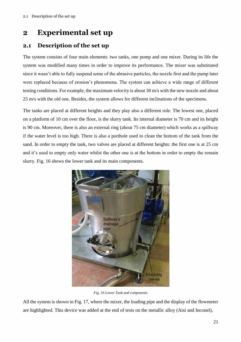
The tanks are placed at different heights and they play also a different role. The lowest one, placed
on a platform of 10 cm over the floor, is the slurry tank. Its internal diameter is 70 cm and its height
is 90 cm. Moreover, there is also an external ring (about 75 cm diameter) which works as a spillway
if the water level is too high. There is also a porthole used to clean the bottom of the tank from the
sand. In order to empty the tank, two valves are placed at different heights: the first one is at 25 cm
and it’s used to empty only water whilst the other one is at the bottom in order to empty the remain
slurry. Fig. 16 shows the lower tank and its main components.
Fig. 16 Lower Tank and components
All the system is shown in Fig. 17, where the mixer, the loading pipe and the display of the flowmeter
are highlighted. This device was added at the end of tests on the metallic alloy (Aisi and Inconel),

2.1 Description of the set up
22
and, up to that moment, the flowrate was computed through pressure measurement, as it’s explained
in the appendix.
Fig. 17 Hydraulic System and components
The water levels in the tanks are chosen such that in the upper tank the nozzle is fully submerged by
water and, in the loading tank, 30 cm of the water are always guaranteed. Choosing a level equal to
70 cm it’s enough for the previous constrain and the total volume in the system is 268 litres, as it’s
clear from Tab. 1.
Tab. 1 System Feature
Tank's Diameter 0.7 m
Water Level 0.7 m
Tank's Volume 261.75 litre
Porthole's Diameter 0.3 m
Porthole's Thickness 0.06 m
Porthole's Volume 4.24 litre
Axle Diameter 0.025 m
Axle Height 0.5 m
Axle Volume 0.245 litre
Impeller Diameter 0.3 m
Impeller Height 0.09 m
Impeller Volume 6.362 litre
Impeller with water Volume 2.12 litre
Total water Volume 267.87 litre
2.1 Description of the set up
23
So, every time the tank is filled up to a level of 70 cm.
The tests are made in the second tank, called test cabine. It contains a nozzle and a support which can
be moved and inclined in many ways. Its height is 70 cm, it has the same spillway and a similar
porthole of the lower one. Besides, the top of the tank can be opened and the bottom is not plane but
it has a conic shape. At the bottom of the cone there’s a hole with a valve which regulates the flow
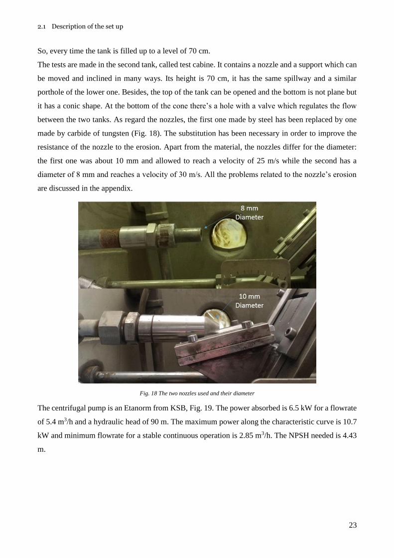
between the two tanks. As regard the nozzles, the first one made by steel has been replaced by one
made by carbide of tungsten (Fig. 18). The substitution has been necessary in order to improve the
resistance of the nozzle to the erosion. Apart from the material, the nozzles differ for the diameter:
the first one was about 10 mm and allowed to reach a velocity of 25 m/s while the second has a
diameter of 8 mm and reaches a velocity of 30 m/s. All the problems related to the nozzle’s erosion
are discussed in the appendix.
Fig. 18 The two nozzles used and their diameter
The centrifugal pump is an Etanorm from KSB, Fig. 19. The power absorbed is 6.5 kW for a flowrate
of 5.4 m3/h and a hydraulic head of 90 m. The maximum power along the characteristic curve is 10.7
kW and minimum flowrate for a stable continuous operation is 2.85 m3/h. The NPSH needed is 4.43
m.

2.1 Description of the set up
24
Fig. 19 Etanorm pump (KSB,2015)
After about 80 tests also the pump broke down (a lot of water started to exit the pump’s cover) and
so it was replaced with a similar one. The breakdown of the pump was caused by the slurry itself.
In Tab. 2, the total amount of sand and the time of usage of the pump with sand is reported.
Tab. 2 Amount of particles and duration before pump’s breakdown
duration [h] kg
Sand Testing 19.26 3312.11
Corundum Testing 2.27 324.02
Pre testing 6.17 801.67
tot 27.70 3636.13
The time for the pre-testing is required in order to bring the system at testing condition, which is more
or less 5 minutes. The following pictures, Fig. 20-Fig. 23, show the amount of erosion of the casing.
All the internal components are made of cast iron.
Fig. 20 Detail of the eroded pump: 3 holes on the volute casing.

2.1 Description of the set up
25
Fig. 21 Entrance of the water and impeller
Fig. 22 Impeller and eroded casing
Fig. 23 Detail of the volute casing

2.1 Description of the set up
26
It’s evident how powerful the erosion can be. The higher damage is observed on the fixed components
of the pump such as the casing, whilst the impeller seems not to be affected by the erosion.
As regard the mixer, its blades are very close to the bottom of the tank and to the side walls (few
millimetres) and a constant rotational speed of 900 rpm is kept during each test. The rpm are
controlled with an inverter.
In the first period a different mixer was used but, since its impeller diameter was smaller (about 15
cm diameter) and it was placed at half-way of the water level, it couldn’t suspend all the abrasive
particles without creating accumulation zones. That’s why a new mixer was chosen.
The exit of the flow in the lower tank was problematic since it carried a lot of air along with it, causing
the pump to go under cavitation. A metallic break-flux was added, as shown in Fig. 28
A mass-flow measuring device, called Coriolis, was initially installed but later removed because the
presence of sand in the fluid was affecting the precision of the its measurements. In the first
configuration, a massic flowrate of 6000 Kg/h was reached.
Beyond the Coriolis, some pipes were also replaced, in order to avoid abrupt curves, thereby reaching
higher jet velocities. These choices enabled the system able to reach a flowrate of 7.5 m3/h and a
velocity at the nozzle’s exit up to 26 m/s or 33 m/s, depending on the nozzle used.
Some valves and gauges are used in order to control the system. The most important ones are shown
in Fig. 24. The system has two lines: the first one is used for the test so that the jet out of the nozzle
is created; the second one is used to fill the upper tank in order to reach the testing conditions, e.g.
nozzle is submerged but not working. Switching between them is possible thanks to a two-way
diverter valve.
For the regulation of the flowrate two control valves can be used: one works with both the lines
(almost hidden in Fig. 24) while the upper one can modify the flow of the second line only and usually
it is not totally open to have the same flowrate exiting from both lines. The pressure can be read with
a manometer, installed in the second line, while the differential pressure gauge, working with the first
line (testing one), is connected to a computer and registers the pressure values with a frequency of
100 Hz.
In Fig. 24 the two-way diverter valve used for the change of the line is indicated as well as the valve
responsible for the control of the water level in the upper tank (and so in the lower one). This is fixed
during the tests and allows to maintain the nozzle submerged and to have a sufficient level in the
lower tank

2.2 Methodology
27
Fig. 24 Control devices and instrumentation of the system
2.2 Methodology
A test starts with fixing the specimen in the desired position.
The specimens are placed in the upper tank of the system where a jet of water mixed with a certain
percentage of solid particles comes out from the nozzle. Inside the tank there is a dedicated support
for the samples, as it can be seen on the left of
Fig. 25. They are secured by screws and nuts.
Fig. 25 Testing camera and its components
Distance screw

2.2 Methodology
28
This kind of configuration is used only for the 90° inclination. The control of the distance (12.7 mm
and 20 mm for GRE) between the nozzle and the metallic specimen is possible thanks to the bigger
screw on the bottom of
Fig. 25, which is adjusted by a small wheel placed outside the tank. For the 15° configuration, it
wasn’t possible to keep the distance of 12.7 mm because of geometrical constrains, i.e. the nozzle
touches the specimen. Therefore, a bigger distance has been set up.
The 90° inclination is the simplest one to be set since it doesn’t require extra support like the other
inclinations. As soon as the distance, the fixing and the angulation of the support are checked, the test
can begin.
An extra support is used in order to set up different inclinations. It’s blocked on the main support and
it has a 45° inclination itself, which makes it possible to achieve all the desired angles without
changing the nozzle-sample distance.
The angle can be changed through a screw whose movement causes the rotation of the main support.
In Fig. 26, the 30° configuration is shown. Besides, an extra cover is added in order to avoid the jet
to direct some water in the spillway, thus affecting the stationarity of the experimental conditions.
Fig. 26 Different inclination configuration
The investigated angles are: 90°, 60°, 30°, 15°.
For the 60° configuration, the extra support is turned by 180°, as shown in Fig. 27.
Inclination
screw

2.2 Methodology
29
Fig. 27 60° configuration: the support is turned
The placement of the specimens, fixed by 4 screws, is such that the flow coming from the nozzle hits
their centre. The same procedure is used for both nozzles.
Once the target materials are placed, the system is run on the second line in order to submerge the
nozzle in the upper tank. In order to maintain a stationary level in the two tanks, the piezometer is
controlled and the valve at the bottom of the testing tank is moved until a stationary condition is
reached.
Then the flow is switched on the testing line and the test can begin. All the data of pressure and
flowrate (when possible) are recorded on the computer using an acquisition model.
While testing, the concentration measurements are made.
The one-litre flask is filled with mixture of water and solid particles: this operation takes place close
to the exit of the flowrate in the lower tank (Fig. 28) and it must be done very carefully for the sample
mixture to be representative of the flowing one. It’s suggested to have the opening of the flask not
completely submerged by the flux. As soon as the flask is filled, it is put on a table where its face is
carefully dried with a paper and then the volume is valued. If two flasks are used, the excess of water
will be put in the 250 ml flask and the relevant volume will be given by the sum of the two flasks.
After the measurement, the flask is emptied in the lower tank.

2.2 Methodology
30
Fig. 28 Exit of the flux from the upper tank: place for concentration sampling
As shown in the above picture, an additional iron sheet has been installed to break the falling flux
which, otherwise, brings a lot of air in the mixture and causes cavitation’s troubles in the pump. The
presence of air is mainly caused by the free surface flux in the pipe between the two tanks.
The next step is the weighing: the flask (or equally the two flasks) is placed on the balance. The mass
of liquid is obtained after subtracting the previously computed tare.
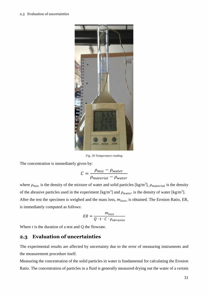
In order to get the density of water, a thermometer is inserted in the bigger flask (Fig. 29) and the
temperature gives the density’s value with the following formula:
𝜌𝑤𝑎𝑡𝑒𝑟 = −0.0063𝑇2 + 0.0609𝑇 + 999.61 [𝑘𝑔
𝑚3]
it’s gained with measurements of water density at temperatures between -30 to 100 C° (David R.
Lide, CRC Handbook of Chemistry and Physics).
On the other hand, the mixture density is given by:
𝜌𝑚𝑖𝑥 =𝑚𝑡𝑜𝑡 − 𝑚𝑡𝑎𝑟𝑒
𝑉 [
𝑘𝑔
𝑚3]
2.3 Evaluation of uncertainties
31
Fig. 29 Temperature reading
The concentration is immediately given by:
𝐶 =𝜌𝑚𝑖𝑥 − 𝜌𝑤𝑎𝑡𝑒𝑟
𝜌𝑚𝑎𝑡𝑒𝑟𝑖𝑎𝑙 − 𝜌𝑤𝑎𝑡𝑒𝑟
where 𝜌𝑚𝑖𝑥 is the density of the mixture of water and solid particles [kg/m3], 𝜌𝑚𝑎𝑡𝑒𝑟𝑖𝑎𝑙 is the density
of the abrasive particles used in the experiment [kg/m3] and 𝜌𝑤𝑎𝑡𝑒𝑟 is the density of water [kg/m3].
After the test the specimen is weighed and the mass loss, 𝑚𝑙𝑜𝑠𝑠, is obtained. The Erosion Ratio, ER,
is immediately computed as follows:
𝐸𝑅 =𝑚𝑙𝑜𝑠𝑠
𝑄 ∙ 𝑡 ∙ 𝐶 ∙ 𝜌𝑎𝑏𝑟𝑎𝑠𝑖𝑣𝑒
Where t is the duration of a test and Q the flowrate.
2.3 Evaluation of uncertainties
The experimental results are affected by uncertainty due to the error of measuring instruments and
the measurement procedure itself.
Measuring the concentration of the solid particles in water is fundamental for calculating the Erosion
Ratio. The concentration of particles in a fluid is generally measured drying out the water of a certain

2.3 Evaluation of uncertainties
32
volume sample and then weighing the solid part. Although it is the most precise, this procedure is
complex and takes a lot of time.
For these reasons, a different procedure was chosen making possible the measurement of the
concentration several times during the same test.
As soon as the system runs steadily the measurements begin: one flask is filled with the flow of water
and particles. This quantity is taken from the point where the mixture coming from the upper tank
returns in the lower reservoir (Fig. 28). It’s assumed that the mean concentration out of the nozzle is
the same at the measuring point.
Flasks, balances and a thermometer were used in order to measure the density.
At the beginning of all the tests, the empty flasks were weighed in order to have the tare’s value. The
balance used is a Diamond model 500 with a precision of 0.5 grams. For the weighing of the full
flasks, the balance used was a Precia Molen m5 with a precision of 1 gram.
The thermometer has a precision of 0.3 °C. Three different flasks were used. In the first tests two
flasks were used simultaneously: one with a capacity of 1 litre and a precision of 0.4 ml and another
one of 250 ml and a precision of 0.5 ml. It was chosen this solution because the 1-liter flask has no
notch but the one indicating one litre: so the excess of water was measured with the smaller flask.
The overall error should be 0.9 ml but it was increased till 1 ml since some extra error could occur
during the transfer of liquid.
In the second period was used only one flask. It has a capacity of 1 litre and notches going from 990
ml to 1100 ml, making the small flask useless and increasing the precision to 0.4 ml.
Later on, a new balance (PCE-BS 3000) is used making possible to increase the accuracy on the mass
to 0.3 gr and the tare is measured with higher precision so it is not considered in error’s propagation.
The next table sums up the precision during the tests.
Tab. 3 Tolerance of the measurement devices
1st set of instruments
2nd set of instruments
3rd set of instruments
δT [°C] 0.3 0.3 0.3
δm [gr] 1 1 0.3
δV [ml] 1 0.4 0.4
The estimation of the uncertainty due to measurement errors is done following the rule of propagation
of the error, which in general is:
𝑢𝑓 = √∑ (𝜕𝑓
𝜕𝑥𝑖𝑢𝑥𝑖
)2𝑛
𝑖=1

2.3 Evaluation of uncertainties
33
The most relevant uncertainty’s values are those ones regarding the concentration and the ER.
𝑢𝑐 = √(𝑢𝜌𝑚𝑖𝑥
𝜌𝑚𝑎𝑡𝑒𝑟𝑖𝑎𝑙 − 𝜌𝑤𝑎𝑡𝑒𝑟)
2
+ ((𝜌𝑚𝑖𝑥 − 𝜌𝑚𝑎𝑡𝑒𝑟𝑖𝑎𝑙) ∗ 𝑢𝜌𝑤𝑎𝑡𝑒𝑟
(𝜌𝑚𝑎𝑡𝑒𝑟𝑖𝑎𝑙 − 𝜌𝑤𝑎𝑡𝑒𝑟)2)
2
Where 𝑢𝜌𝑚𝑖𝑥 and 𝑢𝜌𝑤𝑎𝑡𝑒𝑟
are the uncertainties associated to the density of abrasive material and water,
which are:
𝑢𝜌𝑚𝑖𝑥= √(
𝑢𝑚
𝑉)
2
+ (𝑢𝑉 ∗ 𝑚𝑚𝑖𝑥
𝑉2)
2
𝑢𝜌𝑤𝑎𝑡𝑒𝑟= √(𝑢𝑇 ∗ (−2 ∗ 0.0063 ∗ 𝑇 + 0.0609))2
The uncertainty 𝑢 is given not only by the tolerance of the devices but also their resolutions, ∆, must
be considered (Tab. 4). Looking at the uncertainty on mass 𝑢𝑚 is computed as follows:
𝑢𝑚 = √(𝛿𝑚
√3)
2
+ (∆𝑚
2√3)
2
It is assumed that both the tolerance and the resolution can be descripted with a normal distribution:
the first is included in ±𝛿𝑚 and the latter in ±∆𝑚
2. The same considerations are made for the volume
and the temperature and results for the most precise devices are reported in Tab. 4.
Tab. 4 tolerance, resolution and total uncertainty on the main measured parameters
tolerance 𝜹 Resolution ∆ uncertainty 𝒖
Mass [g] ±0.3 ±0.1 ±0.304
Volume [ml] ±0.4 ±0.5 ±0.471
Temperature [°] ±0.3 ±0.1 ±0.304
In this way, it is possible to assume that the concentration value of a single sample is, for 95% of
probability, inside the range given by the measured concentration ±2𝑢𝑐.
The uncertainty on the mean concentration during a test is investigated, since the mean value is used
for the ER computation. In a test with multiple measurements, the uncertainty around the mean value
must be consider and no more the one concerning the single measurement, 𝑢𝑐 (UNI CEI ENV 13005).
As it is clear in Fig. 30, the concentration is not constant during a test.

2.3 Evaluation of uncertainties
34
Fig. 30 Concentration values during a test
The mean value of N measurements, taken from a Gaussian distribution, can be represented with t
Student distribution (Kottegada and Rosso, 2008).
The mean value and the standard deviation of a test are computed as follows:
𝑐̅ =1
𝑁∑ 𝑐𝑖
𝑁
𝑖=1
𝜎𝑐 = √1
𝑁 − 1∑(𝑐𝑖 − 𝑐̅)2
𝑁
𝑖=1
Where 𝑐𝑖 is a single measure. The standard deviation of the mean value is given by:
𝜎𝑐̅ =𝜎𝑐
√𝑁
It is high for small number of measurements, N.
It can be assumed that the mean concentration of the test 𝑐̅ is included in the range 𝑐̅ ± 𝑡𝑁,95%𝜎𝑐̅ for
a confidence interval of 95%. The percentiles for different degrees of freedom DF are reported in
. The degrees of freedom refer to the number of measurements minus one, N-1.
0.00%
0.10%
0.20%
0.30%
0.40%
0.50%
0.60%
0.70%
0.80%
0.90%
0 2 4 6 8 10 12
Co
nce
ntr
atio
n
Current measurement

2.3 Evaluation of uncertainties
35
Tab. 5 percentile for a two-tail t student distribution
Tab. 6 and Tab. 7 show the results of the use of one or two flasks and the uncertainty of each
measurement and the one on the mean. Tab. 6 refers to a nominal concentration of sand 1% and Tab.
7 to a nominal concentration of corundum 1% with one flask only. Tab. 8 describes a 10 minutes’ test
with sand with a 1% nominal concentration. Where the nominal concentration is the ratio between
the volume of the particles inserted in the lower tank and the volume of water: it is a known value
since these quantities are previously measured and it is the reference value to compare with the
samples.
Tab. 6 30 minutes’ test with sand with two flasks: each line refers to concentration samples at a different increasing time
T [C] ρw[kg/m3] uρw[kg/m3] mmix [kg] V [l] ρmix [kg/m3] uρmix C uC
24.8 997.2 0.025 1.456 1.036 1010.04 1.66 0.85% 0.111%
25.6 997.0 0.026 1.462 1.042 1009.98 1.65 0.86% 0.110%
26.6 996.8 0.027 1.446 1.027 1009.15 1.68 0.82% 0.112%
27.4 996.5 0.028 1.432 1.015 1007.29 1.70 0.71% 0.113%
28.3 996.3 0.030 1.442 1.025 1007.22 1.68 0.73% 0.112%
29.5 995.9 0.031 1.45 1.033 1007.16 1.67 0.75% 0.111%
30.3 995.7 0.032 1.458 1.042 1006.14 1.65 0.70% 0.110%
31.4 995.3 0.033 1.454 1.038 1006.17 1.66 0.72% 0.110%
32.5 994.9 0.035 1.442 1.028 1004.28 1.68 0.62% 0.111%
33.2 994.7 0.036 1.43 1.014 1006.31 1.70 0.77% 0.113%
34.1 994.4 0.037 1.45 1.034 1006.19 1.67 0.79% 0.111%
𝜎𝑐 = 0.07% 𝜎𝑐̅ = 0.02% 𝑡𝑁,95%𝜎𝑐̅ = 0.04%
DF 𝑡𝑁,95%
1 12.706
2 4.303
3 3.182
4 2.776
5 2.571
6 2.447
7 2.365
8 2.306
9 2.262
10 2.228
11 2.201
12 2.179

2.3 Evaluation of uncertainties
36
Tab. 7 5 minutes’ test with corundum with one flask: each line refers to concentration samples at a different increasing time
T [C] ρw[kg/m3] uρw[kg/m3] mmix [kg] V [l] ρmix [kg/m3] uρmix C uC
25.8 996.99 0.02642 1.2580 0.993 1021.45 1.09 0.83% 0.037%
26.5 996.80 0.02730 1.2680 1.001 1023.28 1.08 0.90% 0.037%
27.3 996.58 0.02831 1.2640 0.995 1025.43 1.09 0.98% 0.037%
𝜎𝑐 = 0.07% 𝜎𝑐̅ = 0.04% 𝑡𝑁,95%𝜎𝑐̅ = 0.17%
Tab. 8 10 minutes’ test with sand with one flask: each line refers to concentration samples at a different increasing time
T [C] ρw[kg/m3] uρw[kg/m3] mmix [kg] V [l] ρmix [kg/m3] uρmix C uC
29.5 995.92 0.03108 1.2617 1.006 1012.91 0.50 1.13% 0.033%
30.4 995.64 0.03221 1.2517 0.995 1014.06 0.51 1.22% 0.034%
31.2 995.38 0.03322 1.2627 1.006 1013.91 0.50 1.23% 0.033%
32.1 995.07 0.03436 1.2652 1.007 1015.38 0.50 1.35% 0.033%
32.8 994.83 0.03524 1.2539 1.002 1009.17 0.50 0.95% 0.033% 𝜎𝑐 = 0.15% 𝜎𝑐̅ = 0.07% 𝑡𝑁,95%𝜎𝑐̅ = 0.19%
Where 𝑚𝑚𝑖𝑥 includes the tare, which is 0.4096 kg (2 flasks) and 0.2437 (1 flask). In Tab. 8 the tare
value is not considered in the computation of 𝑢𝜌𝑚𝑖𝑥since its weight was measured more precisely.
As it is clear from the tables, the total error on the concentration is not negligible. Besides, the
concentration is different from the nominal one. Tab. 7 shows a 𝑢𝑐 three times smaller than the one
of Tab. 8. The reason is not only the use of one flask but also the different abrasive material: the
material’s density is at the denominator and so the corundum leads to a smaller error, independently
from the number of flasks used.
As regard the uncertainty on the mean value, it is clear that it depends on the number of measurements
and their dispersion.
The reliability of the measurements is based on the hypothesis that the mean concentration out of the
nozzle is the same as the mean concentration at the exit in the lower tank.
This strong hypothesis has to be verified. It’s based on the fact that the water jet effect out of the
nozzle doesn’t affect the concentration’s values, i.e. there are no accumulation zones in the tanks or
at least their effect is negligible. The only way to check the goodness of the hypothesis is to measure
the concentration directly out of the nozzle and to compare it to the values measured at the exit in the
lower tank.
These tests are performed with sand with a nominal concentration of 1% in volume and with same
conditions of the ER tests: same water level in lower and upper tank, same sampling method (1 litre

2.3 Evaluation of uncertainties
37
flask, balance with precision of 0.3 grams), same flowrate and therefore same velocity (about 30 m/s)
out the carbide of Tungsten nozzle.
In order to sample the mixture directly out of the nozzle in the same testing conditions, some changes
on the system are made. Two different configurations are set up:
• First configuration is a moving one since the pipes are moved for sampling
• Second configuration is a fixed one: sampling doesn’t require any modifications to the set up.
For each configuration, the concentration is sampled both out of the nozzle and in the lower tank in
order to compare these values.
Extra pipes are added directly to the nozzle in order to have the flow exit in the air, making possible
to sample it. In the first configuration are used only plastic pipes to build it, as shown in Fig. 31.
Fig. 31 First configuration in the filling set up: the tank is filled till the submersion of the nozzle
Three pipes with increasing diameter are used in order to have low velocities at the exit, which is
necessary for the measuring. This configuration has an intrinsic problem: the pipes are always
submerged for filling the upper tank whilst, for the measurement, they are moved as shown in Fig.
32. This leads to an alteration of the equilibrium and stationarity in the tank, making the comparison
between the samples in the two tanks uncertain

2.3 Evaluation of uncertainties
38
Fig. 32 First configuration in the sampling set up: the pipes are moved
The second configuration is fixed and there’s no need to move pipes. The configuration doesn’t
change during the tests. Plastic and stainless steel pipes are used and at the end a valve with a big
diameter in order to have small velocity at the exit.
The fixed pipe configuration with the empty tank and during sampling, respectively, are shown in
Fig. 33 and Fig. 34.
Fig. 33 Second configuration in the filling set up: all the pipes are fixed

2.3 Evaluation of uncertainties
39
Fig. 34 Second configuration in the sampling set up same as the filling one: no pipes are moved
In both the alternative configurations, the particle distribution in the tanks is different from each other
and from the testing one. Nevertheless, the key point is that different particle distribution due to
different set ups is not affecting the relation between concentration values in the two sampling points.
Regarding the testing configuration, it’s reasonable to assume that once the effect of the switching of
the line in the flow field is finished, the relation between the samples out of the nozzle and in the
lower tank is similar.
If the concentration values are similar, it can be reasonable assumed that all the measurements at the
exit in the lower tank are reliable in representing the real quantity of particles impacting the target
specimens.
As for all the other samples, the equations used are the following ones:
𝜌𝑤𝑎𝑡𝑒𝑟 = −0.0063𝑇2 + 0.0609𝑇 + 999.61 [𝑘𝑔
𝑚3]
𝜌𝑚𝑖𝑥 =𝑚𝑡𝑜𝑡 − 𝑚𝑡𝑎𝑟𝑒
𝑉 [
𝑘𝑔
𝑚3]
𝐶 =𝜌𝑚𝑖𝑥 − 𝜌𝑤𝑎𝑡𝑒𝑟
𝜌𝑚𝑎𝑡𝑒𝑟𝑖𝑎𝑙 − 𝜌𝑤𝑎𝑡𝑒𝑟
𝑢𝑐 = √(𝑢𝜌𝑚𝑖𝑥
𝜌𝑚𝑎𝑡𝑒𝑟𝑖𝑎𝑙 − 𝜌𝑤𝑎𝑡𝑒𝑟)
2
+ ((𝜌𝑚𝑖𝑥 − 𝜌𝑚𝑎𝑡𝑒𝑟𝑖𝑎𝑙) ∗ 𝑢𝜌𝑤𝑎𝑡𝑒𝑟
(𝜌𝑚𝑎𝑡𝑒𝑟𝑖𝑎𝑙 − 𝜌𝑤𝑎𝑡𝑒𝑟)2)
2
Where the meaning of the factors has already been explained in this work.

2.3 Evaluation of uncertainties
40
In order to compare the results with a ER test, in Tab. 9 the concentration’s values for a test with sand
are reported. These values will be addressed in the next pages and tabs as “test values”.
Tab. 9 Concentration values during a regular test: test values sampled only in the lower tank
T [C] ρ water [kg/m3] m mix [kg] V [l] ρ mix [kg/m3] C 𝑢𝑐
30.2 995.70 1.2465 0.992 1011.89 1.08% 0.0338%
31 995.44 1.2572 1.002 1012.47 1.13% 0.0335%
31.8 995.18 1.2497 0.995 1012.05 1.12% 0.0337%
32.6 994.90 1.2504 0.996 1011.74 1.12% 0.0337%
33.2 994.69 1.2511 0.997 1011.42 1.11% 0.0336%
mean 1.11% 0.034%
std 0.02%
It’s clear that the variation during the test is very small. Besides, the first value is always the most
uncertain because the switch of the line changes the flow field, which need time to reach the steady
state. For this reason, the first value is not used in the following elaborations.
The trend of concentration for the first configuration is shown in Fig. 35. Even though, they are
uncertain because of the movement of the pipe, these values don’t show big difference between the
two points of sampling.
Fig. 35 Comparison between different sampling position in the first configuration and with the test values
The only remarkable conclusion, which can be made, is that the values at the lower tank are higher
than those from the nozzle and that the test values are between the other two: it means that a change
in the configuration can lead to a change in the concentration’s value. Considering the mean values,
the difference between the sampling points is about 28%
0.00%
0.20%
0.40%
0.60%
0.80%
1.00%
1.20%
1.40%
0 1 2 3 4 5
Co
nce
ntr
atio
n
current measurements
First Configuration
Out of the nozzle
Lower Tank
Test values

2.3 Evaluation of uncertainties
41
The most interesting results are from the second configuration, which doesn’t have problems of
variability. In this case the difference between the values at the two points is very small, looking at
the mean values it’s about 0.04%. Besides, not only the concentration values of the two points are
internal in the bands of errors but the test values are within them too.
Fig. 36 Comparison between different sampling position in the second configuration and with the test values
As it is clearly shown in Fig. 36, the values are very similar considering the uncertainty on the
concentration values. This means that taking a sample from the exit in the lower tank is the same as
taking it directly from the nozzle. This is true if a steady state condition is reached and so the sampling
procedure should start after some little time from the switch of the line.
So it has been demonstrated that the concentration measured at the exit in the lower tank is the same
of the concentration out of the nozzle.
Moreover, it’s necessary to check if the “mixture-based” sampling for concentration is reliable or not.
In order to do that, three samples are taken in the same way as usual and the concentration is computed
with the method explained above. Then, the three samples are put in three different containers and
after one day of sedimentation, most of the water is removed and the residual is dried out by heat. In
this way, it’s possible to have all the sand contained in each sample and, weighing it, the concentration
is obtained. The tests are performed with sand and the samples are taken at the exit of the upper tank
in the lower one. The following formulas show the concentration’s computation in the two ways.
𝐶𝑚𝑖𝑥𝑡𝑢𝑟𝑒−𝑏𝑎𝑠𝑒𝑑 =𝜌𝑚𝑖𝑥 − 𝜌𝑤𝑎𝑡𝑒𝑟
𝜌𝑠𝑎𝑛𝑑 − 𝜌𝑤𝑎𝑡𝑒𝑟
𝐶𝑑𝑟𝑖𝑒𝑑 =𝑚𝑎𝑠𝑠𝑠𝑎𝑛𝑑
𝑉 ∙ 𝜌𝑠𝑎𝑛𝑑
0.00%
0.20%
0.40%
0.60%
0.80%
1.00%
1.20%
1.40%
0 1 2 3 4 5
Co
nce
ntr
atio
n
Current measurements
Second Configuration
out of the nozzle
Lower Tank
Test Values

2.3 Evaluation of uncertainties
42
Where the volume V is the same in both the methods and is measured with the one-liter flask with a
precision of 0.4ml. The mass in the dried way is measured with a high precision balance (0.0001 gr)
so it’s reasonable to consider these values not affected by any errors (Tab. 10).
Tab. 10 values for mixture-based and static concentration
Sample T
[C]
ρ water
[kg/m3]
m mix
[kg]
V [l] ρ mix
[kg/m3]
C
[V/V] 𝑢𝑐 tare
[gr]
Sand
[gr]
C
[V/V]
1 20.7 998.17 1.2537 0.998 1013.02 0.99% 0.0391% 9.209 26.606 1.07%
2 29.9 995.80 1.2516 0.995 1013.96 1.21% 0.0392% 8.527 32.089 1.29%
3 33.6 994.54 1.2456 0.990 1013.02 1.23% 0.0394% 8.254 31.894 1.29%
Graphically, the situation is the following, Fig. 37:
Fig. 37 Comparison between dried and mixture-based sampling
As it’s clearly shown, the concentration values are not equal. Nevertheless, the overall deviation
between the two methods is about 5% while the estimated error is about 3,5% in these tests. This very
little difference can be due to sampling errors in the “mixture-based” method, which can however be
considered a very good and reliable way of sampling as well as very fast one.
Even though the differences between dried and mixture-based is positive, it cannot be said that the
mixture-based method underestimates the concentration: many other tests should be performed.
As regard the weighing of the specimens, it’s necessary to have a very good precision since a little
mass loss has to be evaluated. Fig. 38 shows the balance used in the experiments. The model is a
Mettler Toledo AE200: it has a precision of 0.1 mg (0.0001 grams), which is considered to be enough
for the purpose.
0.00%
0.20%
0.40%
0.60%
0.80%
1.00%
1.20%
1.40%
0 1 2 3 4
Co
nce
ntr
atio
n
sample
Comparison of concentration
mixture-based
Dried

2.3 Evaluation of uncertainties
43
Fig. 38 Balance used for specimen weighing (Lab. Diagnostica e Analisi sui Materiali del Costruito – DICA, Politecnico di Milano)
The specimens are weighed before and after the test: every time each sample is cleaned with a piece
of paper soaked with an alcoholic solution in order to remove all the possible dirt which may affect
the weight.
The precision of the balance is high enough to consider negligible the error on the measure compared
with those ones on the concentration and on flowrate.
As already stated for the concentration values, the uncertainty around ER must be considered. The
most affecting quantity is the concentration itself but also the flowrate can have relevant weight, even
though smaller with respect to concentration. In general, the uncertainty is given by:
𝑢𝐸𝑅 = √(𝐸𝑅 ∗ 𝜎𝑐̅
𝐶)
2
+ (𝐸𝑅 ∗ 𝑢𝑄
𝑄)
2
The other quantities in the ER formula are assumed to be measured with very high precision
(particle’s density, duration and mass loss) and their uncertainties do not affect the overall uncertainty
of ER.
Besides, the contribution of Q in the uncertainty can be neglected for high velocity. It’s taken into
account only for velocity of 15 m/s. The 𝑢𝑄 is given by:
𝑢𝑄 = 3.6 ∙ 𝑢𝑝 ∙ (𝑏2 + 4𝑎𝑃)−12⁄ [𝑚3
ℎ⁄ ]

2.4 Materials
44
Where 𝑢𝑝 is the precision of the differential pressure gauge equal to 0.04 bar. The formula comes
from the derivation of the parabola linking Q and P with respect to Q, according to the propagation
of error’s law. The values of a and b are reported in the appendix.
Regarding the final uncertainty on ER, the standard uncertainty is chosen leading to confidence range
as follows:
𝐸𝑅 ± 𝑢𝐸𝑅
Depending on the number of measurements and their variability, the uncertainty on ER is between
5% and 30%.
All the values of ER and the associated errors are reported in the appendix.
2.4 Materials
In this work the behaviour of different target materials under a solid particle impacting flux is
investigated. Different abrasive materials are used in order to study the response of the target to a
changing in dimension and composition of the particles.
For the purpose a silica sand with three different size and corundum are used and as testing material
aluminium, two kind of steel alloy (Aisi 410 and Aisi 4130), Inconel and GRE.
2.4.1 Specimen Materials
The tests are performed on different materials in order to investigate their behaviour in presence of
erosion. A ductile material like the Aluminium is chosen since it is cheap and for its fast erosion
which allows short tests. Stiff steels like Aisi 410 and Aisi 4130 are selected since they are widely
used in machinery components. Inconel is one of the stiffest alloys available. GRE performances are
almost unknown but it is considered an innovative material in the Oil & Gas industry.
Aisi 410, Aisi 4130 and Inconel are used as materials of many valve components in the Oil & Gas
field. Besides, some of these valves have been studied on another hydraulic system at the G. Fantoli
laboratory in the Politecnico of Milan, as described in the chapter “Application: erosion test on a
valve”.
Aluminium 6082
In order to characterize the effect of particles erosion, an extrusion Aluminium alloy EN AW-6082
was selected. The aluminium is chosen as first target material due to its cheap cost, great erosion
which leads to faster tests and because there are some reference data in literature about its erosion
behaviour. This type of alloy is used for structural components and machinery thanks to its good

2.4 Materials
45
mechanical resistance and stiffness. Tab. 11 and Tab. 12 show the chemical and physical properties
of Aluminium, which are found through an online research.
Tab. 11 Properties (http://www.anodallgroup.com/images/files/LEGA_6082.pdf)
Mechanical and physical properties
density [kg/m3] 2700
melting point [C°] 615/655
elastic modulus [Mpa] 69000
tangential elastic modulus [Mpa] 26000
HBW Brinnel 90/95
Tab. 12 Chemical composition (http://www.anodallgroup.com/images/files/LEGA_6082.pdf)
Chemical composition %
silicon Si 0.7-1.3
iron Fe 0.5 max
copper Cu 0.1 max
manganese Mn 0.4-1.0
magnesium Mg 0.6-1.2
chromium Cr 0.25 max
zinc Zn 0.2 max
titanium Tn 0.1 max
others 0.05 each
aluminum 95.2-97
AISI 410
This type of stainless steel has a high resistance to corrosion from atmospheric factors. It’s used in
components of valves and plants, especially in the Oil & Gas industry. Tab. 13 and Tab. 14 show the
chemical and physical properties of AISI 410.
Tab. 13 Properties (http://www.centroinox.it/sites/default/files/pubblicazioni/245A.pdf)
Mechanical and physical properties
Density [kg/m3] 7700
Elastic modulus [Gpa] 215
Resistance to traction Rm [Mpa] 600
HB Brinnel 200
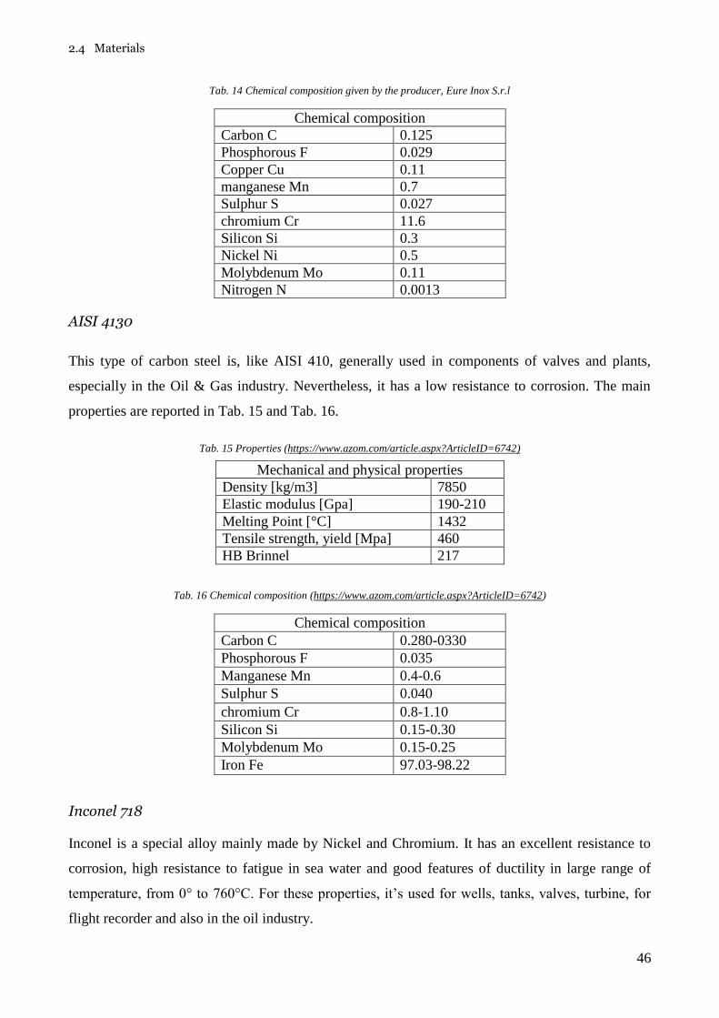
2.4 Materials
46
Tab. 14 Chemical composition given by the producer, Eure Inox S.r.l
Chemical composition
Carbon C 0.125
Phosphorous F 0.029
Copper Cu 0.11
manganese Mn 0.7
Sulphur S 0.027
chromium Cr 11.6
Silicon Si 0.3
Nickel Ni 0.5
Molybdenum Mo 0.11
Nitrogen N 0.0013
AISI 4130
This type of carbon steel is, like AISI 410, generally used in components of valves and plants,
especially in the Oil & Gas industry. Nevertheless, it has a low resistance to corrosion. The main
properties are reported in Tab. 15 and Tab. 16.
Tab. 15 Properties (https://www.azom.com/article.aspx?ArticleID=6742)
Mechanical and physical properties
Density [kg/m3] 7850
Elastic modulus [Gpa] 190-210
Melting Point [°C] 1432
Tensile strength, yield [Mpa] 460
HB Brinnel 217
Tab. 16 Chemical composition (https://www.azom.com/article.aspx?ArticleID=6742)
Chemical composition
Carbon C 0.280-0330
Phosphorous F 0.035
Manganese Mn 0.4-0.6
Sulphur S 0.040
chromium Cr 0.8-1.10
Silicon Si 0.15-0.30
Molybdenum Mo 0.15-0.25
Iron Fe 97.03-98.22
Inconel 718
Inconel is a special alloy mainly made by Nickel and Chromium. It has an excellent resistance to
corrosion, high resistance to fatigue in sea water and good features of ductility in large range of
temperature, from 0° to 760°C. For these properties, it’s used for wells, tanks, valves, turbine, for
flight recorder and also in the oil industry.

2.4 Materials
47
Tab. 17 Properties, ASTM international B637 12
Mechanical and physical properties
Density [kg/m3] 8193
Elastic modulus [Gpa] at 37 °C 205
Melting Point [°C] 1260-
1336 Tensile strength, yield [Mpa] 475
HB Brinnel 331
Tab. 18 Chemical composition, ASTM international B637 12
Chemical composition (%)
Nickel (plus Cobalt) Ni-Co 50-55
Chromium Cr 17-21
Iron Balance
Niobium Nb 4.75-5.50
Molybdenum Mo 2.80-3.30
Titanium Ti 0.65-1.15
Aluminium Al 0.2-0.8
Cobalt Co 1 max
Manganese Mn 0.35 max
Sulphur S 0.015 max
Carbon C 0.08 max
Silicon Si 0.35 max
Boron B 0.006 max
Phosphorous F 0.015 max
Copper Cu 0.30 max
The mechanical and physical properties vary according to the type of alloy and to the corresponding
heat treatment. The features for Inconel-718, which is the most used one, are reported in Tab. 17 and
the chemical composition in Tab. 18.
GRE
Glass Reinforced Epoxy (GRE) is a composite material, whose components are a thermoset polymer
matrix (Epoxy) and glass fiber. Adding glass fiber gives more strength depending on the orientation
of the them. GRE is an innovative material in the Oil & Gas industry and its behaviour under impact
erosion is still not deeply investigated. This material is used as coating for pipes and it is very
interesting for its lower cost, lower thermal conductivity and higher corrosion resistance compared to
the steels. Besides, it has very low roughness which means low head losses as well as low density,
1850 kg/m3, meaning an easier transportability. Unfortunately, no chemical composition and
properties are given by the factory and also the online research has not been successful.

2.4 Materials
48
2.4.2 Abrasive Materials
The abrasive particles’ properties, such as size and hardness, are very important parameters for the
numerical modelling of the erosion as well as for the phenomena itself. Silica sand is chosen because
it’s the most common material and represents the abrasive material that can be found in wells and
pipes in many engineering fields. Instead, Corundum is selected since, after the diamond, is the
hardest material in nature.
Silica sand
The used sands have the same chemical and physical properties except for the size: for simplicity, we
will refer to them as large, medium and thin sand. The use of different granulometry allowed us to
isolate and investigate the effect of the grain size on the ER.
The main properties are reported in Tab. 19 and Tab. 20.
Tab. 19 Properties given by the producer, Sabbie Sataf
Physical properties
density [kg/m3] 2500
bulk density [g/l] 1560
Tab. 20 Chemical composition given by the producer, Sabbie Sataf
Chemical composition %
SiO2 85.7
K2O 0.81
Fe2O3 0.8
BaO 0.12
CaO 0.96
TiO2 0.23
ZrO2 < 0.1
Cr2O3 < 0.1
MgO 1.21
Al2O3 7.95
SO3 0.52
MnO3 < 0.1
NiO < 0.1
SrO < 0.1
The Fig. 39, Fig. 40 and Fig. 41 show the grading curves for each type of sand, given by the producer,
Sabbie Sataf.

2.4 Materials
49
Fig. 39 Large sand grading curve: the dashed lines refer to the maximum and minimum percentage of particles for the diameters
considered
Fig. 40 Medium sand grading curve: the dashed lines refer to the maximum and minimum percentage of particles for the diameters
considered
Fig. 41 Thin Sand grading curve: the dashed lines refer to the maximum and minimum percentage of particles for the diameters
considered
0
10
20
30
40
50
60
70
80
90
100
0 0.2 0.4 0.6 0.8 1
%
mm
0
10
20
30
40
50
60
70
80
90
100
0 0.2 0.4 0.6 0.8 1
%
mm
0
10
20
30
40
50
60
70
80
90
100
0 0.1 0.2 0.3 0.4 0.5 0.6
%
mm

2.4 Materials
50
The commercial features are reported in Tab. 21.
Tab. 21 Mean diameter given by the producer, Sabbie Sataf
Mean diameter (mm)
large 0.35-0.45
medium 0.2-0.35
Thin 0-0.2
Corundum
Corundum RB46’s particles have a sharp-cornered shape with a diameter within 0.355-0.425 mm.
Tab. 22 and Tab. 23 sum up the corundum’s properties.
Tab. 22 Properties (http://www.techmasrl.com/p46/corindone/)
Physical properties
density [kg/m3] 3940
hardness (Mohs) 9
hardness (Knoop) [Kg/mm2] 2400-2500
conductivity [om/cm] 2-6*10-12
Tab. 23 Chemical composition (http://www.techmasrl.com/p46/corindone/)
Chemical composition %
Al2O3 ≥ 93%
TiO2 3
SiO2 0.7
Fe2O3 0.3-0.6
CaO 0.5
Na2O + K2O trace
Free silicon absent

3.1 Tests on Aluminium
51
3. Results
In this section the results of test with different set ups are reported.
3.1 Tests on Aluminium
The aluminium alloy is the most tested material in this work thanks to its fast erosion, which allows
to reduce the duration of the test, and because it is easy to find. Large sand, medium sand, thin sand
and corundum are used as abrasive particles.
Tested inclinations of the specimen are 15°, 30°, 60° and 90°. The durations are 5, 10, 15, 30 minutes.
More than one duration is tested in order to verify its influence on ER
More precisely, all the inclinations are investigated for a velocity of 25m/s with a nominal
concentration of 1% of large sand and corundum. Besides, corundum at 0.3% nominal is used for
each angle and large sand with a velocity of 15 m/s too. At the end, some tests are done with different
sand (large, medium, thin) with a velocity of 30 m/s.
3.1.1 Analysis of the effect of the jet velocity and inclination
The tests with the velocity of the jet equal at 25 m/s are done using two flasks for the concentration
sampling, leading to a precision of 0.11% on the concentration of large sand and the uncertainty on
the ER is around 20%. The tests with a velocity of the jet of 15 m/s are done with only one flask: the
precision on the concentration of large sand is now 0.03% and the uncertainty on ER around 15%.
The values of all the relevant factors are reported in the appendix.
The durations investigated are 5, 10, 15 and 30 minutes as well as 15°, 30°, 60° and 90° inclinations.
In Fig. 42 some eroded specimens are shown: it is clear the influence of the angle of the jet.
Fig. 42 Erosion effect, from right to left: 90°,60, 30° and 15°. Test duration 30 minutes

3.1 Tests on Aluminium
52
Initially, the tests are performed at 90° and only the duration is changed in order to investigate the
time dependence. Later, the angle is changed and the angle-ER function is obtained.
Fig. 43 ER at 90° vs time duration of the test
Fig. 43 shows the ER versus the duration of the test. A significant dependence on time is not
appreciable. Thus for aluminium, the time (and so the geometric changes of the surface) seems to not
affect the ER.
The results show a big uncertainty (up to 20%) on the values of ER at 60°, where the highest
difference between the durations is found, Fig. 44. Nevertheless, a maximum value of ER is found
between 30° and 60°, whilst for air jets it is expected to be between 15° and 40° as it is reported by
Okita et al. (2012) and Oka et al. (1997).
Fig. 44 ER values depending on the angle and duration under a jet velocity of 25 m/s
0.00E+00
2.00E-06
4.00E-06
6.00E-06
8.00E-06
1.00E-05
1.20E-05
1.40E-05
1.60E-05
1.80E-05
0 5 10 15 20 25 30 35
ER [
kg/k
g]
Duration [min]
0.00E+00
5.00E-06
1.00E-05
1.50E-05
2.00E-05
2.50E-05
0 20 40 60 80 100
ER [
kg/k
g]
inclination [°]
10 min
15 min
30 min
5 min

3.1 Tests on Aluminium
53
Normalizing all the values on the ER at 90° the angle function can be drawn, Fig. 45. Only the values
for the 30 minute test are considered, since the values of concentration for these tests show a small
variability between the samples of concentration.
Fig. 45 Normalized values of angle function for ER for 25m/s jet.
Regarding the test with a jet velocity of 15 m/s, it is possible to reach such a velocity thanks to the
control valve. Due to the lower velocity, the error on the flowrate is no more negligible on the ER,
thus it is considered on the computation of the uncertainty.
As usual, all the angles are investigated, the durations are 10 and 20 minutes and the abrasive particle
is large sand.
The values of ER are smaller than those at 25 m/s of almost an order of magnitude, as shown in Fig.
46. Nevertheless, the same trend of the angle dependence is found. Besides, there’s no great difference
between the values for the two different durations.
Fig. 46 ER values depending on the angle with a jet velocity of 25 m/s
The angle function in Fig. 47 confirms that the maximum ER occurs near 30°.
0.00
0.20
0.40
0.60
0.80
1.00
1.20
1.40
0 20 40 60 80 100
ER/E
R9
0[k
g/kg
]
inclination [°]
0.00E+00
5.00E-07
1.00E-06
1.50E-06
2.00E-06
2.50E-06
3.00E-06
3.50E-06
4.00E-06
0 20 40 60 80 100
ER [
kg/k
g]
Inclination [°]
20 min
10 min
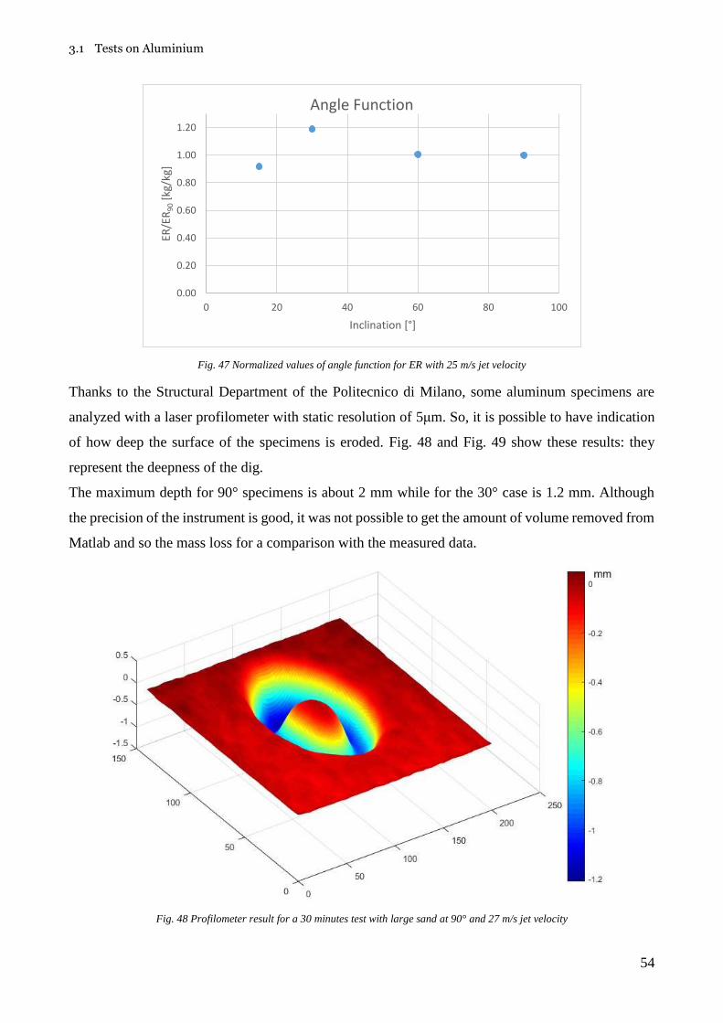
3.1 Tests on Aluminium
54
Fig. 47 Normalized values of angle function for ER with 25 m/s jet velocity
Thanks to the Structural Department of the Politecnico di Milano, some aluminum specimens are
analyzed with a laser profilometer with static resolution of 5μm. So, it is possible to have indication
of how deep the surface of the specimens is eroded. Fig. 48 and Fig. 49 show these results: they
represent the deepness of the dig.
The maximum depth for 90° specimens is about 2 mm while for the 30° case is 1.2 mm. Although
the precision of the instrument is good, it was not possible to get the amount of volume removed from
Matlab and so the mass loss for a comparison with the measured data.
Fig. 48 Profilometer result for a 30 minutes test with large sand at 90° and 27 m/s jet velocity
0.00
0.20
0.40
0.60
0.80
1.00
1.20
0 20 40 60 80 100
ER/E
R9
0[k
g/kg
]
Inclination [°]
Angle Function

3.1 Tests on Aluminium
55
Fig. 49 Profilometer result for a 15 minutes test with large sand at 30° and 25 m/s jet velocity. The arrow points the direction of the
flow
3.1.2 Analysis of the effect of concentration
This set of tests shows a bigger uncertainty due to the variability of the concentration measurements
among the tests. Only the one litre flask is used leading to a precision of 0.04% on the concentration
measurement. As already stated, the angles 15°, 30°, 60° and 90° and the durations of 5, 10 minutes
(only for 0.3% nominal concentration configuration) are investigated. The velocity is the same for all
the test equal to 25 m/s and corundum is the abrasive material.
The small value of nominal concentration chosen lead to higher uncertainty on the single
measurement of concentration: the maximum uncertainty on the ER, computed from the uncertainty
of the mean concentration, is about 25%.
Greater durations where not chosen because of the hardness of corundum: the mineral needs less time
to erode the aluminium compared to Large sand.
The ER as a function of the impact angle is shown in Fig. 50. The behaviour seems different from
that obtained with large sand under the same conditions. Besides, the different abrasive particle can
bring to very dissimilar results because of the different hardness and shape, Kleis and Kulu (2008).
As already said, this set of tests are affected by low precision due to low concentration of corundum.
The ER shows an increasing trend with the angle with the maximum value at 90°.

3.1 Tests on Aluminium
56
Moreover, the difference between the values of the different duration it is still explained by the lower
precision of these test, even though the effect of the geometric changes on the specimen shouldn’t be
excluded a priori.
Fig. 50 ER values depending on the angle for the 0.3% concentration
The tests with a nominal concentration of 1% show a lower uncertainty on the single measurement,
but the error on the concentration measures is now small and so the ER one.
Fig. 51 refers to the ER function of the angle. It is found that the ER of aluminium under corundum
is very similar of that obtained with large sand as abrasive.
Fig. 51 ER values depending on the angle for the 1% configuration
Fig. 52 shows the comparison between the two configurations. It seems that a lower concentration
leads to a bigger ER, especially for higher inclinations, in line with the results of Kleis and Kulu
(2008) for tests in air, even though they remark that the effect of concentration depends also on the
velocity, the angle and the properties of the particles.
0.00E+00
5.00E-06
1.00E-05
1.50E-05
2.00E-05
2.50E-05
3.00E-05
3.50E-05
4.00E-05
4.50E-05
0 20 40 60 80 100
ER [
Kg/
Kg]
inclination [°]
5 min
10 min
0.00E+00
2.00E-06
4.00E-06
6.00E-06
8.00E-06
1.00E-05
1.20E-05
1.40E-05
1.60E-05
1.80E-05
2.00E-05
0 20 40 60 80 100
ER [
kg/k
g]
inclination [°]
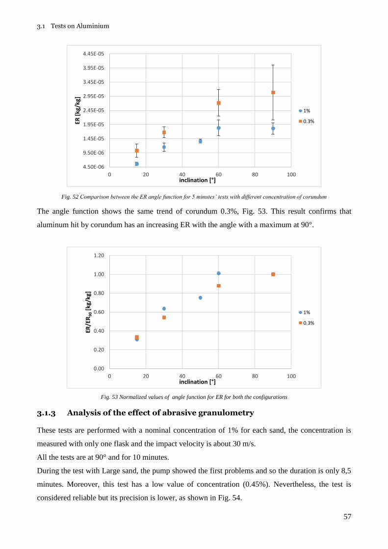
3.1 Tests on Aluminium
57
Fig. 52 Comparison between the ER angle function for 5 minutes’ tests with different concentration of corundum
The angle function shows the same trend of corundum 0.3%, Fig. 53. This result confirms that
aluminum hit by corundum has an increasing ER with the angle with a maximum at 90°.
Fig. 53 Normalized values of angle function for ER for both the configurations
3.1.3 Analysis of the effect of abrasive granulometry
These tests are performed with a nominal concentration of 1% for each sand, the concentration is
measured with only one flask and the impact velocity is about 30 m/s.
All the tests are at 90° and for 10 minutes.
During the test with Large sand, the pump showed the first problems and so the duration is only 8,5
minutes. Moreover, this test has a low value of concentration (0.45%). Nevertheless, the test is
considered reliable but its precision is lower, as shown in Fig. 54.
4.50E-06
9.50E-06
1.45E-05
1.95E-05
2.45E-05
2.95E-05
3.45E-05
3.95E-05
4.45E-05
0 20 40 60 80 100
ER [
kg/k
g]
inclination [°]
1%
0.3%
0.00
0.20
0.40
0.60
0.80
1.00
1.20
0 20 40 60 80 100
ER/E
R9
0[k
g/kg
]
inclination [°]
1%
0.3%
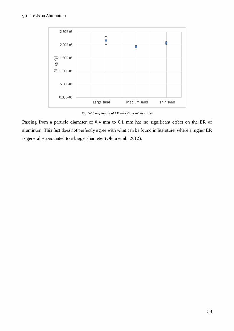
3.1 Tests on Aluminium
58
Fig. 54 Comparison of ER with different sand size
Passing from a particle diameter of 0.4 mm to 0.1 mm has no significant effect on the ER of
aluminum. This fact does not perfectly agree with what can be found in literature, where a higher ER
is generally associated to a bigger diameter (Okita et al., 2012).
0.00E+00
5.00E-06
1.00E-05
1.50E-05
2.00E-05
2.50E-05
ER [
kg/K
g]
Large sand Medium sand Thin sand

3.2 Tests on Aisi 410, Aisi 4130 and Inconel
59
3.2 Tests on Aisi 410, Aisi 4130 and Inconel
The steel alloys are tested because their widespread use in many components of plants and devices.
Large sand, medium sand and thin sand are used as abrasive particles.
Tested inclinations of the specimen are 15°, 30°, 60° and 90° for Aisi 410 hit by medium sand and at
90° for the other targets and abrasives. The durations are 15 and 20 minutes for the two Aisi and 30
minutes for the Inconel.
More precisely, all the inclinations are investigated for a velocity of 30 m/s with a nominal
concentration of 1% of medium sand on the Aisi 410. Besides, all the materials are tested under two
different velocity (25 m/s and 30 m/s) with medium sand as impact material. All the three different
sand sizes are used for the tests on the Aisi, whilst only medium sand and large on Inconel.
All these tests have higher precision on concentration (0.035%) due to the use of only one flask and
a more precise balance and an uncertainty around 10% on ER.
The ER values are computed twice with two different flowrates because it’s not sure which Q-H curve
is the most reliable (see chapter A3). However, the two values are shown only for the angle
dependence for Aisi 410 and they are reported in the final tabs. In all the other graphs the ER values
refer to the lower flowrate.
3.2.1 Analysis of the effect of the jet velocity
In this section the experiments with a nominal concentration of Large sand at 1% in volume and two
jet velocities (25 m/s and 30 m/s) are reported.
The durations investigated on the Aisi are 15 minutes for 25 m/s and 20 minutes for 30 m/s, whilst
the Inconel is tested 30 minutes for both velocities. The inclination is 90° for all the tests.
In Fig. 55 some specimens are shown: on the left, Inconel under 25 and 30 m/s velocity and the same
for Aisi 410 on the right. Even from the picture the difference between the two velocities is clear in
the bigger dig produced by the jet with the higher velocity.
Fig. 55 Eroded specimens: Inconel under 25 and 30 m/s on the left; AISI 410 under 25 and 30 m/s on the right
Fig. 56 report the trend of ER for the different materials and velocities.

3.2 Test on Aisi 410, Aisi 4130 and Inconel
60
Fig. 56 ER for all the steels under different jet velocities
It is clear from Fig. 56 that Inconel is the hardest material: the ER is smaller than in the case of Aisi
steels for both the tested velocities. This confirms that ER depends on the hardness (usually the Brinell
factor) of the target: the smaller the first, the bigger the last, under the same test conditions (Shipway
and Hutchings, 1996).
As regards the Aisi steels, there is no appreciable difference between the two materials since each
result is in the band of error of the other.
3.2.2 Analysis of the effect of the jet inclination
This set of test are made in order to characterize the behaviour of the Aisi 410 under different
inclinations of the jet. The velocity is kept constant and equal to 30 m/s and the duration of test is 20
minutes.
As already stated, the angles are 15°, 30°, 60° and 90° and medium sand is used as abrasive material.
Fig. 57 shows the specimens of Aisi 410 for different angles
Fig. 57 Eroded specimens of Aisi 410: from left to right 15° to 90° inclination. Reference graduation in mm. For the inclined tests the
jet impacts the specimens in the lower part
0.00E+00
1.00E-06
2.00E-06
3.00E-06
4.00E-06
5.00E-06
6.00E-06
7.00E-06
8.00E-06
20.0 22.0 24.0 26.0 28.0 30.0 32.0
ER [
Kg/
kg]
Vjet [m/s]
Aisi 410
Aisi 4130
Inconel

3.2 Test on Aisi 410, Aisi 4130 and Inconel
61
The following figure, Fig. 58, shows the ER trend for different angles. Two values are reported
because an uncertainty in the calculation of the flowrate from the nozzle characteristic curve using
the pressure at the nozzle has risen (see chapter A3).
Fig. 58 ER values depending on the angle
The trend shows that the maximum ER is between 50° and 80° whilst, for tests in air, Kleis and Kulu
(2008) state that the hardened steel has a maximum between 60° and 90°.
0.00E+00
2.00E-06
4.00E-06
6.00E-06
8.00E-06
1.00E-05
1.20E-05
0 20 40 60 80 100
ER [
kg/k
g]
Inclination [°]
AISI 410
v=29.5 m/s
v=33 m/s

3.2 Test on Aisi 410, Aisi 4130 and Inconel
62
3.2.3 Analysis of the effect of abrasive granulometry
The tests are performed with a jet velocity of 30 m/s and the duration the test varies depending on the
target material: 20 minutes for the Aisi and 30 minutes for the Inconel.
Large sand, medium and thin one are used as abrasive for Aisi, whilst only medium sand and large
are tested on Inconel.
Fig. 59, Fig. 60 and Fig. 61 show the eroded specimens with different sizes of the abrasive.
Fig. 59 Erosion Effect on AISI 410: from left to right impacted by large sand, medium and thin
Fig. 60 Erosion Effect on AISI 4130: from left to right impacted by large sand, medium and thin
Fig. 61 Erosion Effect on AISI 410: from left to right impacted by large sand, medium

3.2 Test on Aisi 410, Aisi 4130 and Inconel
63
It can be seen that for the thin sand as a hitting particle, the erode hole is larger respect to the other
ones.
The general trend for all the materials is that the ER decreases with the increasing of grain’s size, Fig.
62.
Fig. 62 Comparison between ER for different sand used
A possible reason is that as the grain size decrease, the flux out of the nozzle impacts a larger area of
the specimen (Fig. 59) with a higher tangential velocity. Besides, the number of impacting particles
is surely higher for smaller grains and perhaps the interaction between the impacting and the bouncing
particles is less important.
Inconel and Aisi 410 show a perfect linear trend: the ER decreases when the grain size is increasing.
Aisi 4130 has a decrease from thin to medium Sand, while it is almost constant between medium and
large sand.
0.00E+00
2.00E-06
4.00E-06
6.00E-06
8.00E-06
1.00E-05
1.20E-05
1.40E-05
ER [
kg/k
g]
Large sand Medium Sand Thin sand
ER
Aisi 410
Aisi 4130
Inconel

3.3 Tests on GRE-Glass Reinforced Epoxy
64
3.3 Test on GRE-Glass Reinforced Epoxy
The Glass Reinforced Epoxy is an innovative material in the Oil & Gas industry and its behavior
under impact erosion is still to be studied.
The test on GRE are performed in the same conditions of the other ones but only thin sand at 1%
nominal is used as abrasive. Besides only 15°, 30° and 90° are investigated for three different
durations of 5, 15 and 30 minutes. The maximum jet velocity reached is 33 m/s but also 21 m/s and
27 m/s are used.
3.3.1 Analysis of the effect of the jet inclination
These tests are performed with different inclination as well as two different velocities of 33 m/s and
21 m/s
The durations investigated are 5, 15 and 30 minutes as well as 15°, 30° and 90° inclinations.
Fig. 63, Fig. 64 and Fig. 65 show some eroded specimen: it is clear the effect of the inclination and
of the time.
Fig. 63 Erosion effect, from right to left: 5, 15 and 30 minutes duration at 15° inclination
Fig. 64 Erosion effect, from right to left: 5, 15 and 30 minutes duration at 30° inclination.

3.3 Tests on GRE-Glass Reinforced Epoxy
65
Fig. 65 Erosion effect, from right to left: 5, 15 and 30 minutes duration at 90° inclination
Looking at the ER values at 33 m/s, a maximum value at 90° is found even though it may be also
between 30° and 90° (Fig. 66).
Fig. 66 ER values at 33 m/s depending on the angle and duration
Moreover, the interesting finding is that if the duration is increased, ER decreases. This can be due to
the effect of the eroded hole evolving during the test. In fact, this is more evident at 90° where the
biggest difference between the holes is found. Nevertheless, other reasons like the changing in the
mechanical properties of the material and the fragmentation of the particles during a test may
contributed to this result.
8.00E-06
1.00E-05
1.20E-05
1.40E-05
1.60E-05
1.80E-05
2.00E-05
2.20E-05
2.40E-05
2.60E-05
0 20 40 60 80 100
ER [
kg/k
g]
Inclination [°]
5 min
15 min
30 min

3.3 Tests on GRE-Glass Reinforced Epoxy
66
As regards the test for a jet velocity of 21 m/s, the ER values are shown in Fig. 67.
Fig. 67 ER at 21 m/s depending on the angle and duration
The ER trend is similar to the one for higher velocity: the possible maximum value of ER is at the
normal angle.
On the other hand, the effect of time, considered as a change of the geometry, is no more so clear as
for 33 m/s case. This is reasonably due to a smaller ER and so to a smaller dig on the target material.
3.3.2 Analysis of the effect of the jet velocity
Three different velocities are tested in order to gain the dependence of the ER on velocity. A jet
velocity of 21 m/s, 27 m/s and 33 m/s is used whilst the durations are 5, 15 and 30 minutes.
Fig. 68 ER dependence on velocity along time
0.00E+00
1.00E-06
2.00E-06
3.00E-06
4.00E-06
5.00E-06
6.00E-06
7.00E-06
0 20 40 60 80 100
ER [
kg/k
g]
Inclination [°]
5 min
15 min
30 min
0.00E+00
1.00E-05
2.00E-05
3.00E-05
4.00E-05
5.00E-05
0.00 5.00 10.00 15.00 20.00 25.00 30.00 35.00 40.00
ER [
kg/k
g]
v [m/s]
5 min
15 min
30 min

3.3 Tests on GRE-Glass Reinforced Epoxy
67
The trend shown in Fig. 68 confirms the previous results: for smaller velocities, the ER values seems
to be similar, while at the higher velocity they differ.
An unexpected trend has been found for the duration of 5 minutes: possible reasons for this behavior
are still to be found.
The change in the geometry affects the trend of the dependency on velocity: a greater influence of
the velocity is related to smaller durations of the tests.
Besides, three test for the same duration (5 minutes) at normal angle and same velocity are done in
order to demonstrate the repeatability of the test.
Fig. 69 Repeatability of the test on the GRE
Fig. 69 shows that the values of ER are equal for each test, confirming its repeatability.
0.00E+00
5.00E-06
1.00E-05
1.50E-05
2.00E-05
2.50E-05
3.00E-05
0 1 2 3 4
ER [
kg/k
g]

4. Discussion of the results
68
4. Discussion of the results
In this section, all the results are compared with each other. From the tests performed, it’s possible to
investigate the effect of the most important parameters of the phenomenon.
A comparison with the literature values is difficult since they mainly refer to air tests. The difference
between single impacts, the air-solid jet tests and the water-solid (slurry) ones must be discussed.
All the erosion models refer to the single-particle condition, which, however, is impossible to
reproduce experimentally. Nevertheless, the single-particle condition is thought to be rather well
reproduced by the abrasive jet impingement test with air, since the high inertia of the particles with
respect to the carrying fluid makes each particle follow almost the same trajectory of the fluid. So, it
is reasonable to assume that 𝑉𝑗𝑒𝑡 ≅ 𝑢𝑝 in air. Most of the literature is based on this consideration.
As regard the test with water, the relation between the velocity of the jet and that of the particles is
not so clear a priori: in this configuration, the particles follow different trajectories of the fluid and
this leads to a spectrum of velocities and impact angles different from what has been called 𝑉𝑗𝑒𝑡 and
θ in chapter 1.
Based on theoretical considerations and tests in air, it is concluded that the ER of a single-particle
[kg/kg] scales with the impact velocity elevated to a certain exponent m. From the literature, the value
of m varies a lot (from 1.6 to 4.1 for different target materials) but the most used value is given by
Oka and the E/CRC as a constant equal to 2.41 for a single particle condition. In reality m depends
also on the impact angle and on the particle features (for high velocities). Since, as already noticed,
the single-particle condition and tests in air are directly related to each other, the following equations
hold and m value is the same:
𝐸𝑅𝑠𝑝~𝑢𝑝𝑚
𝐸𝑅~𝑉𝑗𝑒𝑡𝑚
The above equations also indicate that, for a single-particle condition and tests in air, the ratio between
the ER and the velocity elevated to m should not depend on velocity any longer. Referring to this
ratio makes it possible to compare between the data obtained at different velocities.
The situation is not so clear in case of slurry tests, and, therefore, it was object of investigation in the
present thesis.

4. Discussion of the results
69
Fig. 70 ER dependence on velocity for different target material and same impacting sand
In Fig. 70 only tests at 90° are considered and the abrasive is always large sand. As clearly shown,
the slope for the two Aisi and Inconel is almost the same, whilst the one of Aluminum differs from
them. The next tab shows the error obtained by taking m equal to 2.41 (valid for air according to the
E/CRC model) and the “optimum” m, which leads to the minimum coefficient of variation (Tab. 24).
The error is computed as the ratio between the standard deviation and the mean of the ER’s values
considered.
Tab. 24 Coefficient of variation using m=2.41 and optimum n value
m=2.41
All Aisi 410 Aisi 4130 Inconel
% (σ/μ) 7.69% 8.70% 11.01% 4.69%
optimum m value
n 2.60 1.75 3.24 2.77
Assuming that the uncertainty on the ER alone is between 10% and 20%, the errors produced setting
m=2.41 are acceptable.
Besides, the m values found are quite close to 2.41 for Aluminum and Inconel, while they are very
different for the Aisi. M. Parsi, in his paper - which is a good collection and analysis of many
experimental and numerical results - states that m varies between 1.6 to 2.6 for air tests on metals.
Besides, the dependence on the jet velocity is investigated also for the Thin Sand on Aluminum and
the values are reported in Fig. 71.
0.00E+00
5.00E-06
1.00E-05
1.50E-05
2.00E-05
2.50E-05
0.0 5.0 10.0 15.0 20.0 25.0 30.0 35.0 40.0
ER [
kg/k
g]
Vjet [m/s]
Inconel
AL
Aisi 410
Aisi 4130

4. Discussion of the results
70
Fig. 71 Aluminum dependence on velocity for different impacting sand
Only two velocities are tested but they are enough to find the same behavior of Large sand (2.8 with
thin sand). The trend seems to be not affected by the grain size. Looking at Fig. 7, it’s easy to
understand that the result is reasonable, even though the target material and the carrying fluid are
different. The grain size has an effect on the ER but not on the exponent of the power law 𝐸𝑅 =
𝑎𝑉𝑚(Kleis and Kulu, 2008).
Besides, a comparison with the few literature works that investigate slurry flows is shown in Fig. 72.
Since the conditions of all these tests are different, 𝐸𝑅/𝑉𝑗𝑒𝑡𝑚 is consider for comparing all the values.
The exponent m is chosen equal to 2.41, which is acceptable in slurry flows and it is the most used
value for m in the papers regarding the air-solid jets.
0.00E+00
5.00E-06
1.00E-05
1.50E-05
2.00E-05
2.50E-05
0 5 10 15 20 25 30 35 40
ER [
kg/k
g]
v [m/s]
Aluminum dependence on Velocity
Large sand
Thin sand

4. Discussion of the results
71
Fig. 72 Comparison between scaled ER with literature’s values (Messa et al, 2017)
The GRE shows the most interesting results for the velocity dependence. As reported in the chapter
“Test on GRE-Glass Reinforced Epoxy” the, a change of geometry due to erosion may lead to a
change in the erosion behavior. In Fig. 73, it is clear how different the values for the exponent m are:
the perfectly agree with the founding that the ER decreases with time, meaning that a bigger dig (or
a bigger geometry change) may lead to smaller erosion. Other possible reasons may be the changing
of the mechanical properties of the material and the fragmentation of the particles during the test.
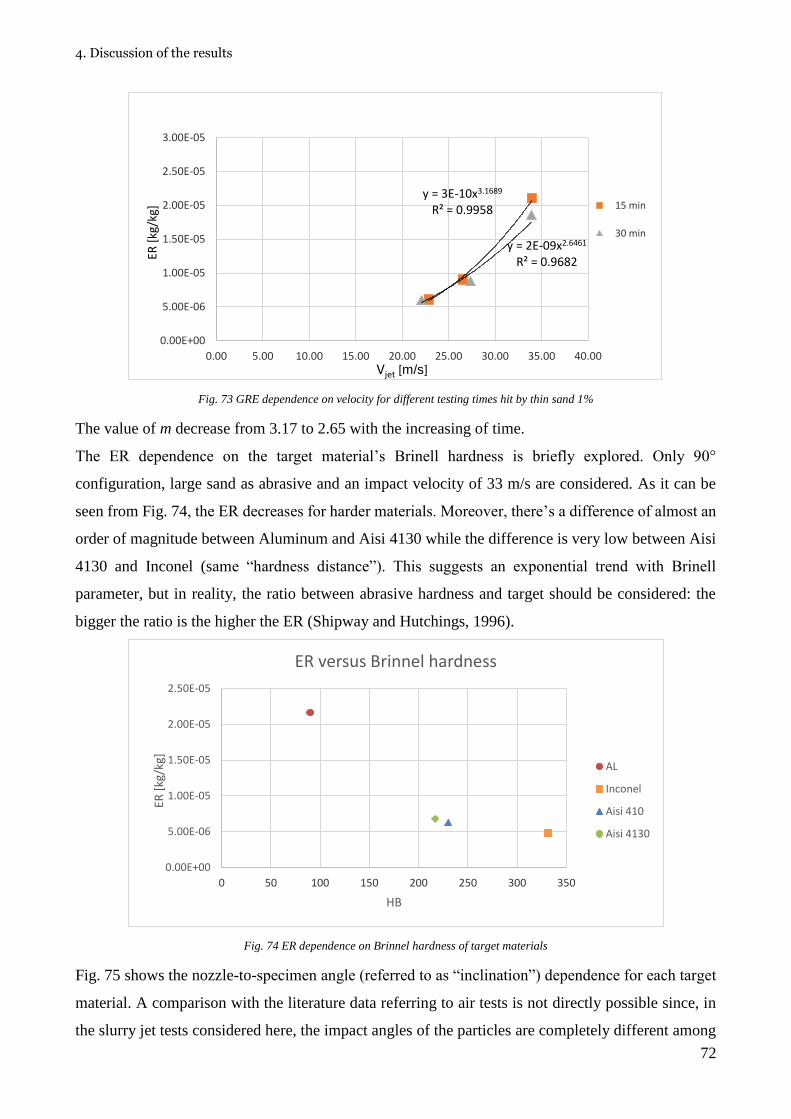
4. Discussion of the results
72
Fig. 73 GRE dependence on velocity for different testing times hit by thin sand 1%
The value of m decrease from 3.17 to 2.65 with the increasing of time.
The ER dependence on the target material’s Brinell hardness is briefly explored. Only 90°
configuration, large sand as abrasive and an impact velocity of 33 m/s are considered. As it can be
seen from Fig. 74, the ER decreases for harder materials. Moreover, there’s a difference of almost an
order of magnitude between Aluminum and Aisi 4130 while the difference is very low between Aisi
4130 and Inconel (same “hardness distance”). This suggests an exponential trend with Brinell
parameter, but in reality, the ratio between abrasive hardness and target should be considered: the
bigger the ratio is the higher the ER (Shipway and Hutchings, 1996).
Fig. 74 ER dependence on Brinnel hardness of target materials
Fig. 75 shows the nozzle-to-specimen angle (referred to as “inclination”) dependence for each target
material. A comparison with the literature data referring to air tests is not directly possible since, in
the slurry jet tests considered here, the impact angles of the particles are completely different among
y = 3E-10x3.1689
R² = 0.9958
y = 2E-09x2.6461
R² = 0.9682
0.00E+00
5.00E-06
1.00E-05
1.50E-05
2.00E-05
2.50E-05
3.00E-05
0.00 5.00 10.00 15.00 20.00 25.00 30.00 35.00 40.00
ER [
kg/k
g]
Vjet [m/s]
15 min
30 min
0.00E+00
5.00E-06
1.00E-05
1.50E-05
2.00E-05
2.50E-05
0 50 100 150 200 250 300 350
ER [
kg/k
g]
HB
ER versus Brinnel hardness
AL
Inconel
Aisi 410
Aisi 4130
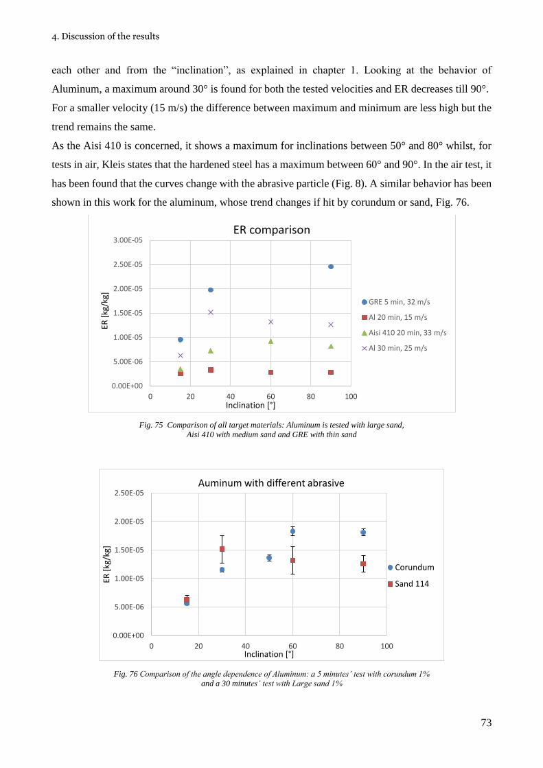
4. Discussion of the results
73
each other and from the “inclination”, as explained in chapter 1. Looking at the behavior of
Aluminum, a maximum around 30° is found for both the tested velocities and ER decreases till 90°.
For a smaller velocity (15 m/s) the difference between maximum and minimum are less high but the
trend remains the same.
As the Aisi 410 is concerned, it shows a maximum for inclinations between 50° and 80° whilst, for
tests in air, Kleis states that the hardened steel has a maximum between 60° and 90°. In the air test, it
has been found that the curves change with the abrasive particle (Fig. 8). A similar behavior has been
shown in this work for the aluminum, whose trend changes if hit by corundum or sand, Fig. 76.
Fig. 75 Comparison of all target materials: Aluminum is tested with large sand,
Aisi 410 with medium sand and GRE with thin sand
Fig. 76 Comparison of the angle dependence of Aluminum: a 5 minutes’ test with corundum 1%
and a 30 minutes’ test with Large sand 1%
0.00E+00
5.00E-06
1.00E-05
1.50E-05
2.00E-05
2.50E-05
3.00E-05
0 20 40 60 80 100
ER [
kg/k
g]
Inclination [°]
ER comparison
GRE 5 min, 32 m/s
Al 20 min, 15 m/s
Aisi 410 20 min, 33 m/s
Al 30 min, 25 m/s
0.00E+00
5.00E-06
1.00E-05
1.50E-05
2.00E-05
2.50E-05
0 20 40 60 80 100
ER [
kg/k
g]
Inclination [°]
Auminum with different abrasive
Corundum
Sand 114

4. Discussion of the results
74
Besides, Fig. 75 shows how big is the difference of ER, which is of one order of magnitude between
GRE and Aluminum compared with the AISI 410, whilst GRE and Aluminum have an ER of almost
the same order of magnitude.
As regard the possibility to infer the brittle or ductile behavior of the target from the inclination curve,
nothing can be stated. In fact, the literature explained in chapter 1 refer to the single particle condition
(or equally with air jet) and the water jet is really different from that condition.
From another point of view, it could be more interesting to have a look on the volumetric erosion ERv
(ratio between removed volume over kg of impacting sand). Its calculation is very easy since it’s
enough to divide the ER by the target material density.
It’s found that the volume losses for Aisi (1 mm3) is the same of Aluminum under an impact velocity
which is half than the Aisi’s one.
For Aluminum exposed to a 25 m/s jet the ERv increases till 5.6 mm3/kg. The GRE has the highest
removal reaching 11.4 mm3/kg at 90°, as shown in Fig. 77.
Fig. 77 ERv comparison for different target materials: Aluminum is tested with large sand,
Aisi 410 with medium sand and GRE with thin sand
Fig. 78 sums up the result regarding the dependence on particle size. The smaller the grains are, the
higher the ER for Aisi and Inconel, while Aluminum shows an almost constant trend. The trend for
the steels is not the expected one but, looking at I. Kleis’s considerations, it’s clear that a universal
trend on the particle’s diameter does not exist even for air test.
0.00
2.00
4.00
6.00
8.00
10.00
12.00
0 20 40 60 80 100
ERv
[mm
3 /kg
]
Inclination [°]
ERv comparison
Al 20 min, 15 m/s
Aisi 410 20 min, 33 m/s
Al 30 min, 25 m/s
GRE 15 min, 33 m/s
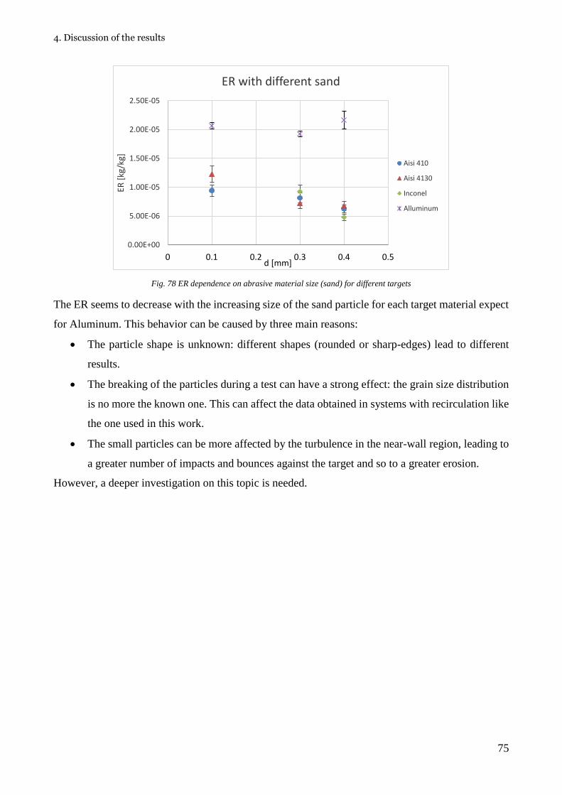
4. Discussion of the results
75
Fig. 78 ER dependence on abrasive material size (sand) for different targets
The ER seems to decrease with the increasing size of the sand particle for each target material expect
for Aluminum. This behavior can be caused by three main reasons:
• The particle shape is unknown: different shapes (rounded or sharp-edges) lead to different
results.
• The breaking of the particles during a test can have a strong effect: the grain size distribution
is no more the known one. This can affect the data obtained in systems with recirculation like
the one used in this work.
• The small particles can be more affected by the turbulence in the near-wall region, leading to
a greater number of impacts and bounces against the target and so to a greater erosion.
However, a deeper investigation on this topic is needed.
0.00E+00
5.00E-06
1.00E-05
1.50E-05
2.00E-05
2.50E-05
0 0.1 0.2 0.3 0.4 0.5
ER [
kg/k
g]
d [mm]
ER with different sand
Aisi 410
Aisi 4130
Inconel
Alluminum

5. Application: erosion test on a valve
76
5. Application: erosion test on a valve
As already explained in the introduction, the characterization of the materials under impact erosion
condition is important for the implementation of the erosion models. The direct impact tests are
fundamental for the characterization of the steels and so the calibration of the erosion models for the
numerical simulations.
Testing the specimens of AISI 410 was the first step, now an applied research is developed on a choke
valve: the investigated component, the cage, is made by AISI 410 too.
Another plant, inside the G. Fantoli laboratory, is used for testing real valves and it’s shown in Fig.
79.
The goals of the tests are to computed the mass loss of the interested component, a qualitative
description of the erosion effects, the control of the flow coefficient CV with the geometrical
evolution due to erosion.
Fig. 79 Erosion Loop system at G.Fantoli Laboratory
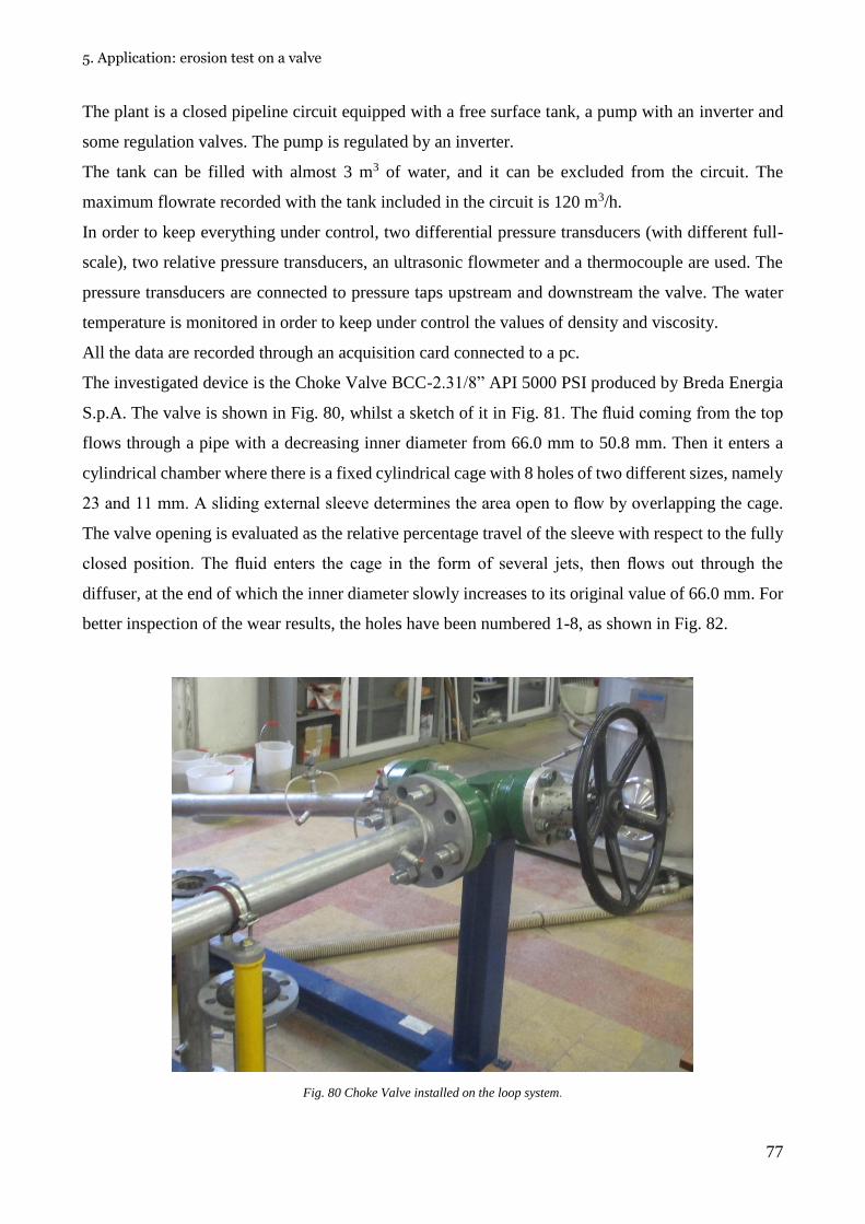
5. Application: erosion test on a valve
77
The plant is a closed pipeline circuit equipped with a free surface tank, a pump with an inverter and
some regulation valves. The pump is regulated by an inverter.
The tank can be filled with almost 3 m3 of water, and it can be excluded from the circuit. The
maximum flowrate recorded with the tank included in the circuit is 120 m3/h.
In order to keep everything under control, two differential pressure transducers (with different full-
scale), two relative pressure transducers, an ultrasonic flowmeter and a thermocouple are used. The
pressure transducers are connected to pressure taps upstream and downstream the valve. The water
temperature is monitored in order to keep under control the values of density and viscosity.
All the data are recorded through an acquisition card connected to a pc.
The investigated device is the Choke Valve BCC-2.31/8” API 5000 PSI produced by Breda Energia
S.p.A. The valve is shown in Fig. 80, whilst a sketch of it in Fig. 81. The fluid coming from the top
flows through a pipe with a decreasing inner diameter from 66.0 mm to 50.8 mm. Then it enters a
cylindrical chamber where there is a fixed cylindrical cage with 8 holes of two different sizes, namely
23 and 11 mm. A sliding external sleeve determines the area open to flow by overlapping the cage.
The valve opening is evaluated as the relative percentage travel of the sleeve with respect to the fully
closed position. The fluid enters the cage in the form of several jets, then flows out through the
diffuser, at the end of which the inner diameter slowly increases to its original value of 66.0 mm. For
better inspection of the wear results, the holes have been numbered 1-8, as shown in Fig. 82.
Fig. 80 Choke Valve installed on the loop system.
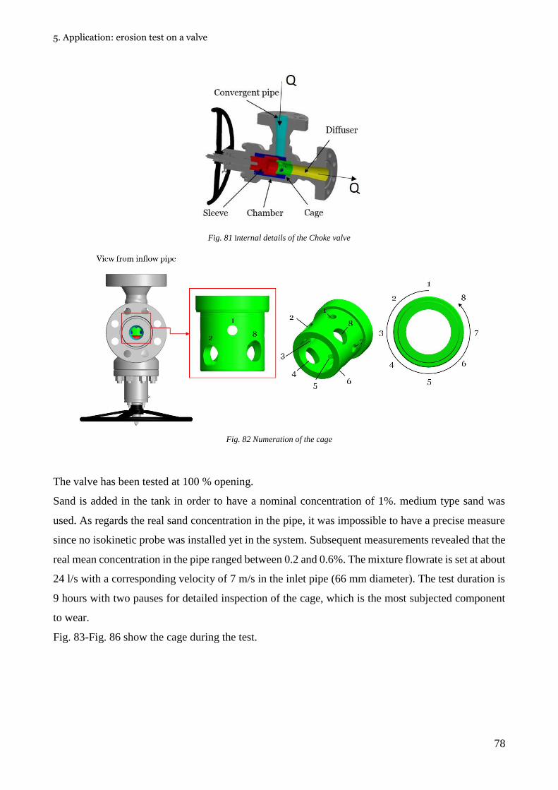
5. Application: erosion test on a valve
78
Fig. 81 Internal details of the Choke valve
Fig. 82 Numeration of the cage
The valve has been tested at 100 % opening.
Sand is added in the tank in order to have a nominal concentration of 1%. medium type sand was
used. As regards the real sand concentration in the pipe, it was impossible to have a precise measure
since no isokinetic probe was installed yet in the system. Subsequent measurements revealed that the
real mean concentration in the pipe ranged between 0.2 and 0.6%. The mixture flowrate is set at about
24 l/s with a corresponding velocity of 7 m/s in the inlet pipe (66 mm diameter). The test duration is
9 hours with two pauses for detailed inspection of the cage, which is the most subjected component
to wear.
Fig. 83-Fig. 86 show the cage during the test.

5. Application: erosion test on a valve
79
Fig. 83 Cage erosion during the tests: view from hole 1
Fig. 84 Cage erosion during the tests: view from hole 3
Fig. 85 Cage erosion during the tests: view from hole 5
Fig. 86 Cage erosion during the tests: view from hole 7
Details of the holes before and after the tests are shown in Fig. 87 and Fig. 88. It is clear the effect of
the sand presence in the water: the edges of the holes are rounded but not equally in each of them.
The two small holes aligned with the inlet (1 and 5), are eroded almost symmetrically. On the other
hand, the rest of holes shows an asymmetrical profile with the scar mainly left-oriented for 6,7, and
8, and right-oriented for 2,3 and 4.
Therefore, erosion is located in the faces opposite to the direction of the flow entering the chamber.

5. Application: erosion test on a valve
80
Fig. 87 Details of the bigger holes (2, 4, 6, 8) before and after the test
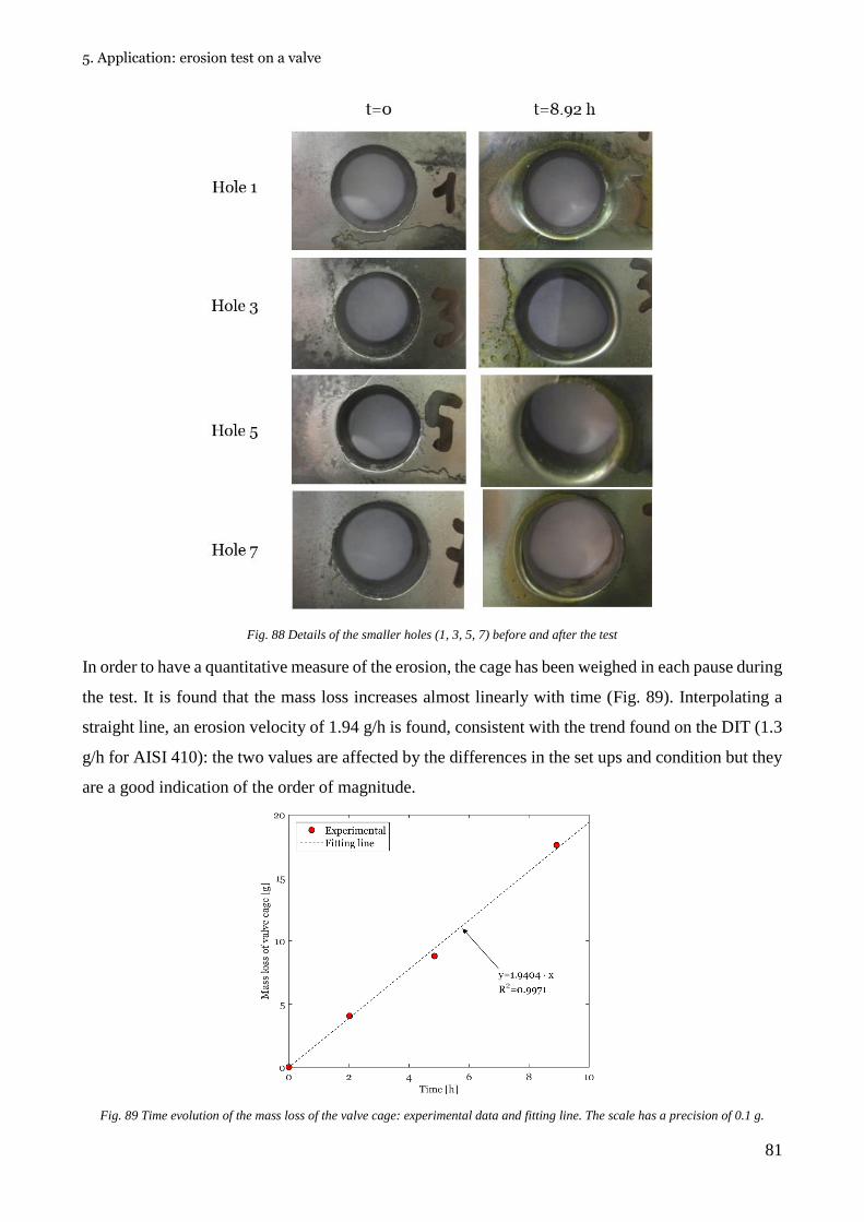
5. Application: erosion test on a valve
81
Fig. 88 Details of the smaller holes (1, 3, 5, 7) before and after the test
In order to have a quantitative measure of the erosion, the cage has been weighed in each pause during
the test. It is found that the mass loss increases almost linearly with time (Fig. 89). Interpolating a
straight line, an erosion velocity of 1.94 g/h is found, consistent with the trend found on the DIT (1.3
g/h for AISI 410): the two values are affected by the differences in the set ups and condition but they
are a good indication of the order of magnitude.
Fig. 89 Time evolution of the mass loss of the valve cage: experimental data and fitting line. The scale has a precision of 0.1 g.

5. Application: erosion test on a valve
82
Besides the mass erosion of the valve, its flow coefficient has been monitored too throughout the
erosion tests. Flow coefficient CV is one of the most important parameter of a valve (IEC 60534-2-
3)
𝐶𝑉 =𝑄
0.865 ∙ √∆𝑝
𝜌𝜌0
⁄
Where the flowrate Q is expressed in m3/h, the pressure drop across the valve ∆𝑝 is in bar, the actual
fluid density 𝜌 and the reference density 𝜌0 are in kg/m3. 𝜌0 is the water density at 15°C. The pressure
drop is evaluated between 2D upstream and 6D downstream the gauge (D is the diameter of the valve
inlet).
The tests for the evaluation of CV of the valve have been performed with constant pressure at the
upstream reference section and decreasing the downstream pressure, in order to increase the flow rate
and the pressure drop. These tests have been performed with fresh water, in between the erosion tests.
The application of the equation above shown, allowed to achieve values of the flow coefficient for
different valve Reynolds numbers and, after discarding the data outside the range of self-similarity
(not completely turbulent flow), it was verified that the largest value is no more than 4% greater than
the smallest one. The flow coefficient characteristic of that valve opening was taken as the arithmetic
mean of the values within the range of self-similarity with respect to the pipe Reynolds number. It
was verified that the maximum uncertainty on pressure and flow rate measurements was below 2%.
For each measurement, the relative error on the flow coefficient was lower than 2.1%.
CV before and after the erosion tests is reported in Fig. 90. Looking at the results obtained, the CV
does not appreciably change and it means that the geometry changes, caused by erosion, are not
enough to affect the regulation characteristics of the valve, at least for this amount of eroded mass.
Fig. 90 Experimentally determined flow coefficient versus pipe Reynolds number before and after the test

6. Conclusions
83
6. Conclusions
This work investigates the problem of the impact erosion of materials from an experimental point of
view. The phenomenon is very relevant in many engineering fields such as oil and gas, where many
components of the plants may be affected by erosion, leading to a decrease in production or even to
a failure of some components, resulting in high economical losses.
After providing an introduction to the erosion problem based on the available literature, (chapter 1),
the experimental apparatus and the computational methodology are described (chapter 2), together
with the target and the abrasive materials used (chapter 3). Finally, the results are reported (chapter 3
and 4) as well as an application in a real geometry of engineering interest (chapter 5).
The main functional dependences of the behaviour of five target materials under impact erosion in
water-solid (slurry) jets has been investigated. In literature, almost all researches consider air as a
carrier fluid, as this is the way to better approach the ideal condition of single impact between a
particle and a surface. Conversely, the erosion produced by slurry jets has been less studied,
contributing to the new approach of this thesis.
Tests were performed for different operating conditions (jet velocities, nozzle-to-inclination angles,
abrasive particles, testing times), and different target materials.
The aluminium 6061 was considered first for its low resistance to erosion and low cost. Aisi 410, Aisi
4130 and Inconel are chosen since they are commonly used for the components of valves and plants,
whilst the Glass Reinforced Epoxy (GRE) is tested because the use of this innovative material is very
promising in the Oil & Gas industry but its resistance to the impact erosion is still not well known.
The Erosion Ratio (ER) of each material (that is, the ratio between the mass loss from the specimen
and the mass of abrasive which has left the nozzle) was determined, and its dependence on the jet
velocity, on the angle between the nozzle and specimen, on the size of the abrasive particles as well
as their hardness was studied. It was found that the ER of aluminium and GRE are similar, i.e. same
order of magnitude, whist the steels show values lower of almost an order of magnitude.
The dependence of ER on the velocity of the water jet is qualitatively similar to that in air jets (that
is, a power law). Conversely, the effect of nozzle-to-specimen inclination is different, probably
because of the different role played by the fluid dynamic interactions between the fluid and the
particles in the two cases.
Moreover, the investigation of the particle size effect showed that larger particles produce lower ER
values. However, the dependence on particle size is worthy of further investigation, since the effect
of this parameter is very complicated and not well understood also for air jets.
The experimental study of the erosion of the valve installed on the E-LOOP pointed out that the mass
loss in time is consistent with the result of the DIT on the same material.
6. Conclusions
84
Besides allowing a preliminary characterization of the slurry erosion of different materials, the results
of this thesis can be used for the development and validation of predictive numerical models. To this
purpose, a deeper investigation on the effect of the test duration should be done as well as a
quantitative analysis of the surface of the eroded surface. Moreover, in order to keep under control
the particle characteristics during the tests (and their possible spurious effects on the experimental
results), a laboratory analysis on the abrasive material at the grain scale and its evolution in time is
needed.

Appendix
85
Appendix
In this section, it is explained how some fundamental parameters are computed and at the end a table
reports all the values and characteristics of each of the 103 tests.
Initially, the device used for the computation of the flowrate, a Coriolis, wasn’t able to work with
slurry. After that, an external magnetic flowmeter was used for calculating the curve of pressure and
flowrate and the flowrate is given by the pressure values measured during the tests. Finally, an
ultrasonic flowmeter was installed and the flowrate was easily taken from it.
Since a characteristic curve of the plant (pressure-flowrate) is measured (next chapter), it is possible
to deduce flowrate by the pressure measurement. A differential pressure transducer is used (Lektra
WT2000DP7S122D with a full-scale of 10 bar and precision is 0.04 bar),. The transducer returns an
electric signal in current, which goes to an acquisition card and then to a computer. Here, thanks to
the software, the instantaneous pressure is recorded.
The pressure is sampled with a frequency of 100 Hz. After any test, these data are elaborated with
Matlab and the mean of all the values is obtained and used in the computation of the flowrate.
Moreover, the nozzle is affected by erosion and so the pressure-flowrate curve need to be calibrate
considering this problem. Two different nozzles are used in this work: one with a diameter of 10 mm
and the other one made by carbide of tungsten with a diameter of 8 mm.

Appendix
86
A.1 Reliability of the pressure-flowrate curve
Initially, the flowrate was computed through the Q-H curve given by the factory of the nozzle (Fig.
91). a brand new nozzle has an exit of 10 mm and an exit angle of 15°. Obviously, the curve was
calculated only with water. Besides, the pressure value is taken 20 cm far from the nozzle. Assuming
that the losses in this little section were small, they were initially neglected.
Fig. 91 Nozzle Q-H curve from the factory
The head losses between the pressure transducer and the nozzle are computed in order to verify the
previous assumption. The aim of this computation is not to obtain the real value of the flowrate (which
it is an interactive process) but to understand how big the head losses are and how much the affect
the computation of the flowrate.
The length of the tubes and their internal diameter are measured in order to model the distributed and
localized losses. Fig. 92 and Tab. 25 show the main features and calculations. Three different values
of flowrate are considered: 1.8, 2 and 2.2 l/s.
y = 0.7044x1.9985
0.0
20.0
40.0
60.0
80.0
100.0
120.0
0 2 4 6 8 10 12 14
Hyd
rau
lic H
ead
[m
]
Flowrate [m3/h]

Appendix
87
Fig. 92 Detail of the pipes between nozzle and pressure gauge
Tab. 25 Losses between nozzle and pressure guage. Each line refers to three velocity chosen: 1.8 l/s, 2 l/s and 2.2 l/s
1) STRICTURE D20-D16.5 2) DISTRIBUTED PRESSURE DROP D16.5 3) WIDENING D16.5-D21.5
k [-] D
[mm] V [m/s] ΔH [m] D [mm] ε/D [-] V [m/s] Re [-] λ [-] L [m] JL [m] k [-] D [mm] V [m/s] ΔH [m]
0.15 16.5 8.42 0.54 16.5 0.00273 8.42 1.4E+05 0.026 0.02 0.12 0.2 21.5 4.96 0.25
0.15 16.5 9.35 0.67 16.5 0.00273 9.35 1.5E+05 0.026 0.02 0.14 0.2 21.5 5.51 0.31
0.15 16.5 10.29 0.81 16.5 0.00273 10.29 1.7E+05 0.026 0.02 0.17 0.2 21.5 6.06 0.37
5) STRICTURE D21.5-20 4) DISTRIBUTED PRESSURE DROP D21.5 7) WIDENING D20-D20.5
0.1 20 5.73 0.17 21.5 0.00209 4.96 1.1E+05 0.025 0.02 0.03 0.1 20.5 5.45 0.15
0.1 20 6.37 0.21 21.5 0.00209 5.51 1.2E+05 0.025 0.02 0.04 0.1 20.5 6.06 0.19
0.1 20 7.00 0.25 21.5 0.00209 6.06 1.3E+05 0.025 0.02 0.04 0.1 20.5 6.67 0.23
9) STRICTURE D20.5-D17.2 6) DISTRIBUTED PRESSURE DROP D20
0.15 17.5 7.48 0.43 20 0.00225 5.73 1.1E+05 0.025 0.04 0.09
0.15 17.5 8.32 0.53 20 0.00225 6.37 1.3E+05 0.025 0.04 0.11
0.15 17.5 9.15 0.64 20 0.00225 7.00 1.4E+05 0.025 0.04 0.13
8) DISTRIBUTED PRESSURE DROP D20.5
20.5 0.00220 5.45 1.1E+05 0.025 0.09 0.17
20.5 0.00220 6.06 1.2E+05 0.025 0.09 0.21
20.5 0.00220 6.67 1.4E+05 0.025 0.09 0.26
10) DISTRIBUTED PRESSURE DROP D17.2
17.2 0.00262 7.75 1.3E+05 0.026 0.04 0.19
17.2 0.00262 8.61 1.5E+05 0.026 0.04 0.23
17.2 0.00262 9.47 1.6E+05 0.026 0.04 0.28
The following formulas are used for the losses computation:

Appendix
88
Stricture and widening: 𝑘 ∙𝑉2
2𝑔 and k varies with the ratio d/D.
Distributed drop: 𝑅𝑒 =𝜌𝑣𝐷
𝜇 where 𝜌 = 999 𝑘𝑔/𝑚3 and 𝜇 = 0.001004 𝑝𝑎 𝑠. For the friction factor
the Haaland’s formula is used. 1
√𝜆= −1.8 ∙ log [(
𝜀𝐷⁄
3.7)
1.11
+6.9
𝑅𝑒]
Summing up:
Tab. 26 Head Loss and flowrate estimation
Q [l/s] Q [m3/h] Hydraulic Head [m]
ΔHtot [m]
1.8 6.48 29.50 2.13 2 7.2 36.41 2.63
2.2 7.92 44.05 3.18
For the supposed flowrates, which cover the range of the normal activity, the head losses are about
2-3 meters (Tab. 26) and the flowrate is not the one given by the factory curve. this uncertainty on
the flowrate values may affect heavily the computation of the erosion rate. For this reason, a
calibration of the of Q-H curve of the nozzle is required.
Moreover, after some tests it is noticed that as time passes the pressure upstream the nozzle decreases.
Firstly, the temperature seemed to be the cause, but when the nozzle was taken apart, because a little
piece of a seal had caused anomalous pressure value, it was clear that the nozzle was eroded, Fig. 93.
Fig. 93 Comparison of a used nozzle (left) and a new one (right)

Appendix
89
Fig. 93 shows the difference between a brand new nozzle (on the right) and a nozzle used for 8.6
hours. As it is clear, the opening is wider and the internal holes are eroded.
Hence, the pressure-flowrate curve of the plant changes because of the nozzle erosion and must be
constantly checked.
A new pressure-flowrate curve is needed as well as its calibration due to erosion problems.
A.2 Calibration of the 10mm nozzle
In order to have a precisely calculation of the flowrate from the pressure measurement, new Q-H
curves are computed.
A magnetic flowmeter with a full-scale of 2.2 l/s which is enough for the system is used. The model
is Toshiba 335/379 and it has precision of 0.4%.
The flowmeter is external and for its use the delivery pipe is changed with the one including the
instrument.
Since the flowmeter can work only with water, it is assumed that there is no significant difference in
the pressure-flowrate curve between a water flux and a slurry flow at low concentration. Moreover,
the new curves take into account the position of the pressure transducer and there are no more losses
to be modelled.
Both the flowmeter and the pressure transducer send to the computer an electrical input in current
which is automatically converted in the physical quantities.
These tests were made starting from the maximum value of flowrate (all the valves open) and then
decreasing it with a gradual closing of the flow valve. For each condition, a 20 second acquisition is
done and the test stopped when the pressure reached values smaller than 1 bar.
Two preliminary tests were done in order to verify that the same curve occurs for a submerged nozzle
condition and another one for not submerged. From Fig. 94 it’s clear that there is no difference
between the configurations.
Fig. 94 Comparison between curves by submerged and not submerged nozzle

Appendix
90
Three further tests were done: one with a brand new nozzle, one with a nozzle used for 8.617 hours
and 10.617 hours with water and sand.
Fig. 95 Comparison of Q-H curves for different time use of the nozzle
In Fig. 95 four curves are represented: it is immediately clear that the factory curve is not similar to
the one obtained with a brand new nozzle. Besides, the effects of the erosion can be seen: there is an
increase of flowrate for the same pressure values caused by the erosion of the nozzle.
At the beginning, only the data of the new and 8 hours used nozzle are analysed. The data are
interpolated with a second-degree polynomial and a linear interpolation of the coefficients of the
parabola versus time is obtained from these equations (Fig. 96): with a known time of use of the
nozzle and the pressure measurement is now possible to have a more precise flowrate value.
Tab. 27 Values of the parabola coefficients
parabola's coefficients
t use [h] a b
0 0.9717 -0.0075
8.671 0.871 -0.1594
Fig. 96 Variation with time of the parabola coefficients
Summing up, the flowrate is given by:
y = 0.9717x2 - 0.0075xR² = 1
y = 0.871x2 - 0.1594xR² = 0.9977
y = 0.8092x2 - 0.1144xR² = 0.9981
0
0.5
1
1.5
2
2.5
3
3.5
4
4.5
5
0.5 1 1.5 2 2.5
Hydra
ulic
Haed [
bar]
Flowrate [l/s]
Q-H curves
Brand New
Used 8 ore
Factory curve
U2 Used 10 ore
Polin. (Brand New)
Polin. (Used 8 ore)
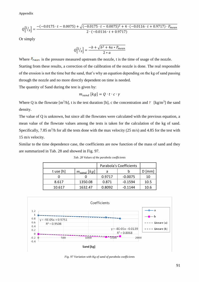
Appendix
91
𝑄[𝑙𝑠⁄ ] =
−(−0.0175 ∙ 𝑡 − 0.0075) + √(−0.0175 ∙ 𝑡 − 0.0075)2 + 4 ∙ (−0.0116 ∙ 𝑡 + 0.9717) ∙ 𝑃𝑚𝑒𝑎𝑛
2 ∙ (−0.0116 ∙ 𝑡 + 0.9717)
Or simply
𝑄[𝑙𝑠⁄ ] =
−𝑏 + √𝑏2 + 4𝑎 ∗ 𝑃𝑚𝑒𝑎𝑛
2 ∗ 𝑎
Where is the pressure measured upstream the nozzle, t is the time of usage of the nozzle.
Starting from these results, a correction of the calibration of the nozzle is done. The real responsible
of the erosion is not the time but the sand, that’s why an equation depending on the kg of sand passing
through the nozzle and no more directly dependent on time is needed.
The quantity of Sand during the test is given by:
𝑚𝑠𝑎𝑛𝑑 [𝑘𝑔] = 𝑄 ∙ 𝑡 ∙ 𝑐 ∙ 𝛾
Where Q is the flowrate [m3/h], t is the test duration [h], c the concentration and [kg/m3] the sand
density.
The value of Q is unknown, but since all the flowrates were calculated with the previous equation, a
mean value of the flowrate values among the tests is taken for the calculation of the kg of sand.
Specifically, 7.85 m3/h for all the tests done with the max velocity (25 m/s) and 4.85 for the test with
15 m/s velocity.
Similar to the time dependence case, the coefficients are now function of the mass of sand and they
are summarized in Tab. 28 and showed in Fig. 97.
Tab. 28 Values of the parabola coefficients
Parabola's Coefficients
t use [h] 𝑚𝑠𝑎𝑛𝑑 [𝑘𝑔] a b D [mm]
0 0 0.9717 -0.0075 10
8.617 1350.08 0.871 -0.1594 10.5
10.617 1632.47 0.8092 -0.1144 10.6
Fig. 97 Variation with Kg of sand of parabola coefficients

Appendix
92
From these data, the flowrate is now computed as:
𝑄[𝑙𝑠⁄ ] =
−(−8.033 ∙ 10−5 ∙ 𝑆𝑎𝑛𝑑 − 0.0139) + √(−8.033 ∙ 10−5 ∙ 𝑆𝑎𝑛𝑑 − 0.0139)2 + 4(−9.167 ∙ 10−5 ∙ 𝑆𝑎𝑛𝑑 + 0.9751) ∙ 𝑃𝑚𝑒𝑎𝑛
2 ∙ (−9.167 ∙ 10−5 ∙ 𝑆𝑎𝑛𝑑 + 0.9751)
In Tab. 28 the variation of nozzle diameter is also reported. This value is important for the
computation of velocity at the exit of the nozzle. Fig. 98 shows the variations depending on Sand Kg.
Fig. 98 Nozzle diameter variation with Kg of sand
Moreover, this method is used for any type of experiment, neglecting the different abrasive material.
A.3 Calibration of the 8mm nozzle
As for the 10 mm nozzle, the calibration is done measuring pressure and flowrate. The flowrate was
initially computed with the magnetic flowmeter and after with the ultrasonic one. Besides, at 5.64
hours of testing the pump was changed, but the curve remained the same (Fig. 99). It must be
underlined that the curves do not change among 5.6, 6.2 and 8.15 hours, meaning that no erosion of
the nozzle occurs during this period of time. After an accurate check of the nozzle diameter with a
calipers and an elaboration of nozzle’s photo with autocad and matlab, it can be said that the diameter
is still 8 mm.
For the 10 mm nozzle the difference between the curves was observed for each curve computed and
this was due to the erosion of the nozzle.
In this case the difference between the brand new nozzle curve and the succesive ones is hard to
explain, since no widening of the nozzle is visible and no appreciable change in the pressure- flowrate
curve occurs from t=5.64 h to t=15 h (Fig. 100). This may be due to the limescale of sand furred up
in the pipes, since the system had been stopped for some days before the change of the nozzle.
This fact has a great influence on the test uncertainty before the installation of the ultrasonic
flowmeter, specifically all the test with Aisi 410, Aisi 4130 and Inconel. For these materials the
erosion ratio changes wheter if computed with the brand new curve or the other one.
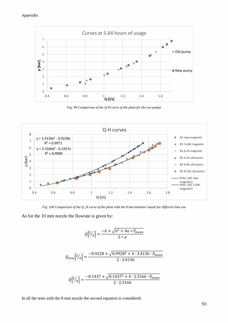
Appendix
93
Fig. 99 Comparison of the Q-H curve of the plant for the two pumps
Fig. 100 Comparison of the Q_H curve of the plant with the 8 mm diameter nozzle for different time use
As for the 10 mm nozzle the flowrate is given by:
𝑄[𝑙𝑠⁄ ] =
−𝑏 + √𝑏2 + 4𝑎 ∗ 𝑃𝑚𝑒𝑎𝑛
2 ∗ 𝑎
𝑄𝑛𝑒𝑤[𝑙𝑠⁄ ] =
−0.9228 + √0.99282 + 4 ∙ 3.4136 ∙ 𝑃𝑚𝑒𝑎𝑛
2 ∙ 3.4136
𝑄[𝑙𝑠⁄ ] =
−0.1437 + √0.14372 + 4 ∙ 2.3166 ∙ 𝑃𝑚𝑒𝑎𝑛
2 ∙ 2.3166
In all the tests with the 8 mm nozzle the second equation is considered.
0
1
2
3
4
5
6
7
0.4 0.6 0.8 1 1.2 1.4 1.6
p [
bar
]
Q [l/s]
Curves at 5.64 hours of usage
Old pump
New pump
y = 3.4136x2 - 0.9228xR² = 0.9971
y = 2.3166x2 - 0.1437xR² = 0.9989
0
1
2
3
4
5
6
7
8
0.4 0.6 0.8 1 1.2 1.4 1.6 1.8
p [
bar
]
Q [l/s]
Q-H curves
N1 new magnetic
N1 5.64h magnetic
N1 6.2h magnetic
N1 6.2h ultrasonic
N1 6.4h ultrasonic
N1 8.15h ultrasonic
Polin. (N1 newmagnetic)Polin. (N1 5.64hmagnetic)

Appendix
94
A.4 Comparison between different flowmeters
After a lot of tests, an ultrasonic flowmeter was installed on a vertical pipe. In order to verify the Q-
H curves computed with the previous devices, a simultaneous acquisition of pressure and flowrate
with both the ultrasonic and magnetic flowmeter is performed. In Fig. 101 the two curves are shown
and the difference between them can be considered negligible.
Fig. 101 System Q-H curve by different devices
The small differences are due to the different precision of the instruments: the magnetic flowmeter is
more precise than the ultrasonic one. Nevertheless, the deviation of the ultrasonic flowmeter is at
maximum of 1.5 % with respect to the magnetic flowmeter. An external flowmeter (the ultrasonic
one) makes possible the measurement of the flowrate during a test without using the Q-H curves. As
it is clear in the following Fig. 102 and Fig. 103, the ultrasonic flowmeter is able to measure correctly
even with a slurry flow. The variability seems to increase with the presence of sand, but the standard
deviation around the mean value for each step of Q [l/s] is still low.
Fig. 102 System Q-H curve measured by Ultrasonic flowmeter, in case of water and slurry flow
0
1
2
3
4
5
6
7
8
0.9 1.1 1.3 1.5 1.7
P [
bar
]
Q [l/s]
slurry 1%
Water

Appendix
95
Fig. 103 Standard deviation of flowrate in case of water and slurry flow.
These curves refer to the new nozzle with a diameter of 8 mm
Appendix B
Tab. 29 report of all the tests and main parameters’ values
Specimen name
Specimen material
Abrasive material
incl. [°]
conc. nom.
[% vol]
conc. meas. [% vol]
Jet velocity
[m/s] duration
[min] distance
[mm]
mass loss [mg]
ER [kg/kg]
𝒖𝑬𝑹 [𝒌𝒈/𝒌𝒈]
GRE 1 gre thin sand 30 1.00 0.92% 33.73 0.01 20.0 0.02900 1.48E-03 5.40E-05
GRE 2 gre thin sand 30 1.00 1.04% 33.18 5 20.0 0.25570 1.97E-05 3.12E-06
GRE 4 gre thin sand 30 1.00 1.00% 33.26 15 20.0 0.6913 1.83E-05 3.99E-06
GRE 5 gre thin sand 30 1.00 0.97% 33.27 30 20.0 1.1941 1.63E-05 2.07E-06
GRE 7 gre thin sand 15 1.00 0.94% 33.80 5 21.0 0.1137 9.52E-06 9.31E-07
GRE 9 gre thin sand 90 1.00 0.73% 33.90 30 20.0 1.0402 1.86E-05 5.7E-07
GRE 8 gre thin sand 15 1.00 0.83% 33.90 15 21.0 0.3172 9.92E-06 3.59E-07
GRE 6 gre thin sand 15 1.00 0.89% 33.81 30 21.0 0.6007 8.85E-06 2.89E-07
GRE 10 gre thin sand 90 1.00 0.80% 33.45 5 20.0 0.2485 2.46E-05 4.48E-06
GRE 11 gre thin sand 90 1.00 0.75% 33.95 15 20.0 0.6059 2.11E-05 8.83E-07
GRE25 gre thin sand 15 1.00 1.23% 21.06 30 21.0 0.1974 3.37E-06 2.33E-07
GRE 12 gre thin sand 15 1.00 1.30% 20.98 15 21.0 0.0673 2.18E-06 2.93E-07
GRE 13 gre thin sand 15 1.00 1.26% 21.86 5 21.0 0.0216 2.07E-06 6.54E-08
GRE 14 gre thin sand 30 1.00 1.18% 21.41 30 20.0 0.2284 4.01E-06 1.14E-07
GRE 15 gre thin sand 30 1.00 1.15% 21.37 15 20.0 0.1169 4.19E-06 2E-07
GRE 16 gre thin sand 30 1.00 1.14% 21.88 5 20.0 0.0327 3.47E-06 2.7E-07
GRE 17 gre thin sand 90 1.00 1.06% 22.07 30 20.0 0.3163 5.98E-06 1.9E-07
GRE 18 gre thin sand 90 1.00 1.00% 22.85 15 20.0 0.1568 6.07E-06 2.34E-07
GRE 19 gre thin sand 90 1.00 1.04% 22.58 5 20.0 0.0544 6.16E-06 4.87E-07
GRE 20 gre thin sand 90 1.00 0.89% 27.48 5 20.0 0.39713 4.3E-05 5.31E-06
GRE 21 gre thin sand 90 1.00 0.89% 26.53 15 20.0 0.2407 9.03E-06 6.43E-07
GRE 22 gre thin sand 90 1.00 0.90% 27.34 30 20.0 0.4915 8.82E-06 3.28E-07
GRE 23 gre thin sand 90 1.00 0.86% 34.91 5 20.0 0.2456 2.16E-05 9.62E-07
0
0.002
0.004
0.006
0.008
0.01
0.012
0.014
0.9 1.1 1.3 1.5 1.7
Qst
d [
l/s]
Q [l/s]
Slurry 1%
Water

Appendix
96
GRE 24 gre thin sand 90 1.00 0.81% 35.21 5 20.0 0.23387 2.16E-05 2.01E-07
GRE 26 gre thin sand 90 1.00 0.90% 35.15 5 20.0 0.26183 2.19E-05 6.02E-08
Al 14 all large sand 90 1.0 0.89% 27.03 5 12.7 0.14687 1.01E-05 1.26E-06
Al 06 all large sand 90 0.5 0.39% verificare 30 12.7 0.60583 1.63E-05 9.81E-07
Al 05 all large sand 90 1.0 1.46% verificare 30 12.7 1.77856 1.30E-05 2.07E-06
Ac 01 acc large sand 90 1.0 0.99% verificare 30 12.7 0.45159 4.84E-06 1.17E-06
Al 08 all large sand 90 1.0 1.08% verificare 30 12.7 0.73642 7.39E-06 1.08E-06
Al 10 all large sand 90 1.0 0.96% verificare 30 12.7 0.74722 8.29E-06 1.74E-06
Al 18 all large sand 90 1.0 0.75% 27.60 30 12.7 0.79880 1.08E-05 1.62E-06
Al 17 all large sand 90 1.0 0.99% 27.34 30 12.7 0.97297 9.95E-06 1.11E-06
Al 13 all large sand 90 1.0 1.15% 27.08 15 12.7 0.46817 8.34E-06 1.39E-06
Al 11 all large sand 90 1.0 0.83% 27.01 5 12.7 0.1277 9.45E-06 1.26E-06
Al 12 all large sand 90 1.0 0.83% 27.05 15 12.7 0.3724 9.15E-06 1.23E-06
Al 16 all large sand 90 1.0 0.16% 26.79 5 12.7 0.0286 1.11E-05 7.76E-06
Al 19 all large sand 90 1.0 0.36% 26.84 15 12.7 0.2222 1.26E-05 3.88E-06
Al 20 all large sand 90 1.0 0.85% 26.81 15 12.7 0.5823 1.40E-05 1.71E-06
Al 21 all large sand 90 1.0 1.23% 26.62 5 12.7 0.20207 1.01E-05 9.27E-07
Al 22 all large sand 90 1.0 0.96% 26.61 5 12.7 0.19227 1.24E-05 1.44E-06
Al 23 all large sand 90 1.0 0.88% 26.53 15 12.7 0.5404 1.26E-05 6.68E-07
Al 24 all large sand 90 1.0 0.92% 26.43 30 12.7 1.1033 1.22E-05 1.4E-06
Al 25 all large sand 90 1.0 0.86% 26.32 30 12.7 1.0942 1.29E-05 1.05E-06
Al 26 all large sand 90 1.0 0.82% 26.23 10 12.7 0.331 1.24E-05 1.97E-06
Al 27 all large sand 90 1.0 0.79% 26.23 10 12.7 0.3212 1.24E-05 3.94E-06
Al 28 all large sand 15 1.0 0.78% 25.96 15 23.5 0.3011 7.80E-06 4.68E-07
Al 31 all large sand 15 1.0 0.79% 25.94 30 23.5 0.4875 6.21E-06 3.14E-07
Al 32 all large sand 15 1.0 0.72% 25.90 10 23.5 0.1549 6.55E-06 4.11E-07
Al 35 all large sand 30 1.0 0.71% 25.86 30 12.7 1.0664 1.51E-05 7.66E-07
Al 33 all large sand 30 1.0 0.83% 25.87 10 12.7 0.3704 1.36E-05 4.58E-07
Al 34 all large sand 30 1.0 0.88% 25.78 15 12.7 0.56073 1.29E-05 8.60E-07
Al 37 all large sand 60 1.0 0.43% 25.80 10 12.7 0.2804 1.95E-05 3.63E-07
Al 39 all large sand 60 1.0 0.60% 25.81 30 12.7 0.7875 1.32E-05 2.16E-06
Al 40 all large sand 60 1.0 0.50% 25.77 15 12.7 0.3612 1.44E-05 1.05E-06
Al 41 all corundum 90 0.3 0.22% 26.95 10 12.7 0.2786 2.53E-05 1.53E-06
Al 42 all corundum 90 0.3 0.15% 26.94 5 12.7 0.116 3.08E-05 7.20E-07
Al 43 all corundum 15 0.3 0.18% 26.90 10 16.85 0.1051 1.16E-05 4.51E-06
Al 44 all corundum 15 0.3 0.21% 26.90 5 16.9 0.0536 1.03E-05 8.72E-07
Al 45 all corundum 30 0.3 0.15% 26.87 10 12.7 0.1484 1.91E-05 2.96E-06
Al 46 all corundum 30 0.3 0.17% 26.85 5 12.7 0.0718 1.67E-05 9.69E-06
Al 47 all corundum 60 0.3 0.14% 26.86 10 12.7 0.1603 2.27E-05 9.36E-06
Al 48 all corundum 60 0.3 0.11% 26.85 5 12.7 0.0778 2.71E-05 2.33E-06
Al 49 all corundum 90 1.0 1.08% 26.63 5 12.7 0.4875 1.81E-05 6.30E-06
Al 50 all corundum 60 1.0 0.90% 26.59 5 12.7 0.41313 1.83E-05 1.89E-06
Al 51 all corundum 30 1.0 1.23% 26.49 5 12.7 0.3542 1.15E-05 2.39E-06
Al 53 all corundum 15 1.0 1.18% 26.37 5 15.75 0.789 2.70E-05 4.69E-06
Al 54 all corundum 15 1.0 1.29% 26.34 5 17.2 0.17977 5.61E-06 1.27E-05

Appendix
97
Al 55 all corundum 50 1.0 0.96% 26.36 5 12.7 0.3252 1.36E-05 2.00E-06
Al 56 all large sand 15 1.0 1.30% 15.18 20 15.4 0.1312 2.56E-06 2.77E-06
Al 57 all large sand 15 1.0 1.18% 15.04 10 15.4 0.0552 2.39E-06 1.49E-06
Al 58 all large sand 30 1.0 1.22% 15.28 20 12.7 0.1611 3.31E-06 1.13E-06
Al 60 all large sand 30 1.0 1.18% 15.49 10 12.7 0.0797 3.32E-06 5.26E-07
Al 62 all large sand 60 1.0 1.18% 15.23 20 12.7 0.1321 2.80E-06 6.69E-07
Al 63 all large sand 60 1.0 1.13% 15.12 10 12.7 0.0633 2.82E-06 2.22E-07
Al 64 all large sand 90 1.0 1.07% 15.29 20 12.7 0.12 2.78E-06 5.48E-07
Al 65 all large sand 90 1.0 0.97% 15.57 10 12.7 0.0621 3.11E-06 3.81E-07
Aisi 410 1 Aisi 410 large sand 90 1.0 0.88% 29.92 15 12.7 0.2086 7.0E-06 2.86E-07
Aisi 4130 1 Aisi 4130 large sand 90 1.0 0.83% 29.87 15 12.7 0.2118 7.6E-06 2.01E-07
IN 3 Inconel large sand 90 1.0 0.70% 29.78 30 12.7 0.2527 5.3E-06 1.97E-07
AISI 410 2 Aisi 410 large sand 90 1.0 0.72% 25.22 20 12.7 0.1367 5.0E-06 2.20E-07
IN 2 Inconel large sand 90 1.0 0.64% 25.12 30 12.7 0.1141 3.1E-06 3.69E-07
AISI 4130 2 Aisi 4130 large sand 90 1.0 0.66% 25.15 17.43 12.7 0.1012 4.1E-06 7.2E-07
Al 69 all large sand 90 1.0 0.42% 29.62 8.37 12.7 0.1688 2.2E-05 9.8E-07
AISI 4130 6 Aisi 4130 sand THIN 90 1.0 0.98% 29.66 20 12.7 0.5996 1.4E-05 2.6E-07
AISI 410 3 Aisi 410 sand THIN 90 1.0 1.05% 29.71 20 12.7 0.4958 1.1E-05 1.8E-06
Al 71 All sand THIN 90 1.0 1.06% 29.70 10 12.7 0.4887 2.1E-05 2.3E-07
Al 73 All sand THIN 90 1.0 1.11% 25.21 10 12.7 0.2612 1.2E-05 2.9E-07
IN 1 Inconel medium
sand 90 1.0 1.18% 29.46 30 12.7 0.8148 1.0E-05 5.7E-06
Al 70 All medium
sand 90 1.0 1.19% 29.54 10 12.7 0.5109 1.9E-05 3.5E-07
AISI 410 8 Aisi 410 medium
sand 90 1.0 1.27% 29.48 20 12.7 0.5141 9.1E-06 5.4E-07
AISI 4130 11 Aisi 4130
medium sand 90 1.0 1.12% 29.49 20 12.7 0.4014 8.1E-06 2.1E-06
AISI 410 7 Aisi 410 medium
sand 60 1.0 0.92% 29.50 20 12.7 0.4188 1.0E-05 2.7E-07
AISI 410 10 Aisi 410 medium
sand 30 1.0 0.98% 29.47 20 12.7 0.3525 8.1E-06 6.6E-07
AISI 410 9 Aisi 410 medium
sand 20 1.0 0.99% 29.51 15 23 0.1709 3.9E-06 3.3E-06

References
98
References
R.J.K. Wood, D.W. Wheeler, “Design and performance of a high velocity air–sand jet impingement
erosion facility”, Wear 220 (1998), 95–112.
M. Parsi, K. Najmi, F. Najafifard, S. Hassani, B.S. McLaury and S.A. Shirazi, “A comprehensive
review of solid particle erosion modeling for oil and gas well sand pipelines applications”, Journal of
Natural Gas Science and Engineering 21 (2014), 850-873.
S. Malavasi, G.V. Messa and L. Piani, “A numerical-experimental investigation of the impact erosion
of Glass Reinforced Epoxies (GRE)”, AIMETA XXIII conference (2017).
G.V. Messa, Y. Wang, L. Piani and A. Malavasi “Numerical simulation of impact erosion in liquid-
solid abrasive jet impingement tests”, ECCOMAS YIC (2017).
I. Kleis, P. Kulu, “Solid particle erosion occurrence, prediction and control”, Springer-Verlag London
Limited (2008).
A. Mansouri, H. Arabnejad, S.A. Shirazi, and B.S. McLaury, “A combined CFD/experimental
methodology for erosion prediction”, Wear 332-333 (2015), 1090-1097.
Girish R. Desale, Bhupendra K. Gandhi and S.C. Jain, “Particle size effects on the slurry erosion of
aluminium alloy (AA 6063)”, Wear 266 (2009), 1066-1077.
P. Shipway and I. Hutchings, “The role of particle properties in the erosion of brittle materials”, Wear
193 (1996), 105-113.
H. Arabnejad, S.A. Shirazi, B.S. McLaury, H.J. Subramani and L.D. Rhyne, “The effect of erodent
particle hardness on the erosion of stainless steel”, Wear 332-333 (2015), 1098-1103
V.B. Nguyen, Q.B. Nguyen, Z.G. Liu, S. Wan, C.Y.H. Lim, Y.W. Zhang, “A combined numerical-
experimental study on the effect of surface evolution on the water-sand multiphase flow
characteristics and the erosion behavior”, Wear 319 (2014) 96-109.
R. Okita, Y. Zhang, B.S. McLaury and S.A. Shirazi, “Experimental and computational investigations
to evaluate the effects of fluid viscosity and particle size on erosion damage”, Journal of Fluids
Engineering (2012), vol.134.
A. Mansouri, S.A. Shirazi and B.S. McLaury, “Experimental and numerical investigation of the effect
of viscosity and particle size on the erosion damage caused by solid particles”, ASME FEDSM
(2014), Paper No. 21613.
Y.I. Oka, K. Okamura, T. Yoshida,” Practical estimation of erosion damage caused by solid particle
impact Part1: effect of impact parameters on a predictive equation”, Wear 259 (2005) 95–101.
A.K. Jha, R. Batham, M. Ahmed, A.K. Majumder, O.P. Modi, S. Chaturvedi, A.K Gupta,” Effect of
impinging angle and rotating speed on erosion behavior of aluminum”, Trans. Nonferrous Met. Soc.
China 21 (2011) 32-38.
N.T. Kottegoda and R. Rosso, “Applied Statistics for civil and environmental engineers”, Blackwell
(2008)