EXPERIMENTAL ASSESSMENT OF AGGREGATES by A thesis

EXPERIMENTAL ASSESSMENT OF AGGREGATES

by

Nicholas Robert Trimble

A thesis submitted in partial fulfillment of the requirements for the degree

of

Master of Science

in

Civil Engineering

MONTANA STATE UNIVERSITY Bozeman, Montana

July 2007

© COPYRIGHT

by


2007

All Rights Reserved

ii

APPROVAL

of a thesis submitted by


This thesis has been read by each member of the thesis committee and has been found to be satisfactory regarding content, English usage, format, citations, bibliographic style, and consistency, and is ready for submission to the Division of Graduate Education.

Dr. Robert L. Mokwa

Approved for the Department of Civil Engineering

Dr. Brett W. Gunnink

Approved for the Division of Graduate Education

Dr. Carl A. Fox

iii

STATEMENT OF PERMISSION TO USE

In presenting this thesis in partial fulfillment of the requirements for a master’s

degree at Montana State University, I agree that the Library shall make it available to

borrowers under rules of the Library.

Copying is allowable only for scholarly purposes, consistent with “fair use” as

prescribed in the U.S. Copyright Law. Requests for permission for extended quotation

from or reproduction of this thesis in whole or in parts may be granted only by the

copyright holder.

Nicholas Robert Trimble July 2007

iv

ACKNOWLEDGEMENTS

The author extends his appreciation to family and friends for their support

throughout the course of preparing this thesis. The author would also like to thank Bob

Mokwa and Eli Cuelho for their valuable advice, guidance, and patience throughout the

testing and writing that went into the preparation of this thesis.

Recognition is also extended to Montana Department of Transportation personnel

in obtaining soil samples from around the state, and to Mike Mullings for conducting all

R-value tests.

Acknowledgement of financial support for this research is extended to the

Western Transportation Institute and the Montana Department of Transportation.

v

TABLE OF CONTENTS

1. INTRODUCTION..................................................................................................... 1

2. MATERIALS ............................................................................................................ 4

3. AGGREGATE MATERIALS TESTING................................................................. 9

Statistical Evaluation of Results................................................................................ 9 Particle Size Distribution ........................................................................................ 11 Modified Proctor Compaction................................................................................. 15 Relative Density ...................................................................................................... 17 Specific Gravity....................................................................................................... 19 Los Angeles Abrasion ............................................................................................. 20 Resistance Value ..................................................................................................... 21

4. DIRECT SHEAR .................................................................................................... 24

Background ............................................................................................................. 24 Testing Conditions .................................................................................................. 26

Apparatus and Sample Preparation ............................................................ 26 Compacted Density of Samples ................................................................. 26

Results ..................................................................................................................... 27 Friction Angle ............................................................................................ 29 Initial Stiffness ........................................................................................... 32 Secant Stiffness .......................................................................................... 33

Summary ................................................................................................................. 35

5. PERMEABILITY.................................................................................................... 36

Testing Conditions .................................................................................................. 37 Apparatus ................................................................................................... 37 Sample Preparation .................................................................................... 39 Testing Procedure....................................................................................... 42

Results ..................................................................................................................... 45 Estimating Permeability from Grain Size ............................................................... 46

Background ................................................................................................ 46 Results ........................................................................................................ 50

Void Ratio-Permeability Relationships................................................................... 53 Summary ................................................................................................................. 59

6. X-RAY COMPUTED TOMOGRAPHY ................................................................ 60

vi

TABLE OF CONTENTS - CONTINUED

History & Applications ........................................................................................... 60 Acquiring Images: How it Works .......................................................................... 62 Apparatus and Scanner Setup.................................................................................. 65 Sample Preparation ................................................................................................. 67 Image Processing..................................................................................................... 67

Despeckling................................................................................................ 68 Thresholding .............................................................................................. 68

Void Ratio Analysis ................................................................................................ 74 Grain Size Analysis ................................................................................................. 75 Pore Size Analysis................................................................................................... 79 Estimating Permeability from Pore Size Distribution............................................. 81

Background ................................................................................................ 81 Results ........................................................................................................ 82

Summary ................................................................................................................. 84

7. SUMMARY & CONCLUSIONS ........................................................................... 85

REFERENCES........................................................................................................ 89

APPENDICES......................................................................................................... 92

APPENDIX A. MDT Grain Size Distribution Analysis Plots ............................... 93 APPENDIX B. R-value Test Reports .................................................................... 96 APPENDIX C. Shear Stress-Displacement Plots ................................................ 111 APPENDIX D. Despeckled 2D X-ray CT Images............................................... 115 APPENDIX E. X-ray CT Grain Size Plots .......................................................... 128

vii

LIST OF FIGURES Figure Page 1. Location map showing origin of samples. ..................................................................... 5

2. Pictures of CBC-6A samples from a) Butte, b) Missoula, c) Glendive, d) Billings, e) Great Falls, and f) Kalispell. ................................................................................. 7

3. Pictures of CBC-5A samples from a) Missoula, b) Great Falls, and c) Kalispell. ........ 7

4. Pictures of CTS-2A samples from a) Missoula, b) Billings, c) Glendive, d) Lewistown, and e) Havre. ..................................................................................... 8

5. p-value ranges utilized in this study for the two sample t-test..................................... 11

6. MDT specification limits for CBC-5A, CBC-6A, and CTS-2A.................................. 12

7. CBC-6A gradation results from the MSU soils lab. .................................................... 13

8. CBC-5A gradation results from the MSU soils lab. .................................................... 14

9. CTS-2A gradation results from MSU soils lab............................................................ 14

10. CTS-2A modified Proctor and maximum index density comparison........................ 16

11. Maximum and minimum index density test results. .................................................. 18

12. Schematic Diagram of a Stabilometer (from Huang 2004). ...................................... 22

13. R-value test results..................................................................................................... 22

14. Direct shear testing apparatus a) mold halves, b) mold placed in load frame with a crane, c) vibratory compactor, and d) assembled mold halves with air bladder and cover plate attached to top. ............................................................................... 25

15. Void ratio (e) for each direct shear test compared to emax and emin. ........................... 27

16. Example of strength parameter (ki, ku, and σu) determination. .................................. 28

17. Mohr-Coulomb failure envelopes for 6A samples: a) Butte, b) Missoula, c) Glendive, d) Billings, e) Great Falls, and f) Kalispell. ....................................... 29

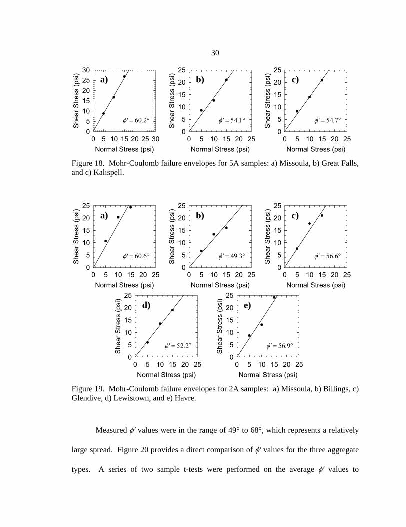
18. Mohr-Coulomb failure envelopes for 5A samples: a) Missoula, b) Great Falls, and c) Kalispell........................................................................................................ 30

19. Mohr-Coulomb failure envelopes for 2A samples: a) Missoula, b) Billings, c) Glendive, d) Lewistown, and e) Havre. .............................................................. 30

20. Internal friction angles (φ′) for each aggregate. ......................................................... 31

viii

LIST OF FIGURES - CONTINUED Figure Page 21. Initial stiffness (ki) results. ......................................................................................... 32

22. Secant stiffness (ku) results. ....................................................................................... 34

23. Photograph and schematic diagram of permeameter setup........................................ 37

24. Support plate for bottom of specimen mold. ............................................................. 39

25. Schematic diagram of permeameter base and specimen mold. ................................. 42

26. Schematic diagram of permeameter fully assembled. ............................................... 43

27. Summary of permeability (k) test results. .................................................................. 45

28. Calculated permeabilities for the 6A aggregates. ...................................................... 51



31. Void ratio versus permeability for all aggregates in this study. ................................ 54

32. Phase diagrams illustrating e, ec, and ef for the same soil (Modified from Cote and Konrad 2003).................................................................................................... 55

33. Conceptual schematic views of a) uneven fines distribution and b) even fines distribution. ............................................................................................................. 56

34. Fine fraction void ratio (ef) versus permeability. ....................................................... 57

35. Schematic plan view of MSU 3rd generation CT scanner......................................... 63

37. 2D slice CT images reconstructed using: a) two views, b) four views, c) eight views, d) 16 views, e) 32 views, and f) 64 views (from Russ 2002). ..................... 65

38. Thresholding example: a) original image, b) thresholded image, and c) pixel intensity histogram with threshold value indicated on the x-axis. .......................... 69

39. Thresholding example where void pixels in identified solid areas are minimized: a) original image, b) thresholded image, and c) pixel intensity histogram with threshold value indicated on the x-axis. .................................................................. 70

40. Threshold sensitivity plots for: a) 2A-Billings, b) 6A-Missoula, c) 6A-Billings, d) 6A-Kalispell, and e) 5A-Great Falls. .................................................................. 73

41. X-ray CT and weight-volume void ratio comparison. ............................................... 75

ix

LIST OF FIGURES - CONTINUED Figure Page 42. Image processing steps before grain size analysis: a) despeckled image,

b) thresholded image, c) image after closing and removal of misclassified void pixels. .............................................................................................................. 77

43. Grain size distributions determined by mechanical sieving and X-ray CT images for the 5A-Missoula sample. ................................................................................... 78

44. CBC-6A pore size distributions. ................................................................................ 79

45. CBC-5A pore size distributions. ................................................................................ 80

46. CTS-2A pore size distributions.................................................................................. 80

47. Pore size of 80% passing (p80) versus permeability (k) plot...................................... 83

A 1. CBC-6A gradation results from MDT soils lab. ...................................................... 94



B 1. R-value test report for 6A-Missoula......................................................................... 97

B 2. R-value test report for 6A-Glendive......................................................................... 98

B 3. R-value test report for 6A-Billings........................................................................... 99

B 4. R-value test report for 6A-Great Falls.................................................................... 100

B 5. R-value test report for 6A-Butte............................................................................. 101

B 6. R-value test report for 6A-Kalispell....................................................................... 102

B 7. R-value test report for 5A-Missoula....................................................................... 103

B 8. R-value test report for 5A-Kalispell....................................................................... 104

B 9. R-value test report for 5A-Great Falls.................................................................... 105

B 10. R-value test report for 2A-Havre. ........................................................................ 106

B 11. R-value test report for 2A-Glendive..................................................................... 107

B 12. R-value test report for 2A-Missoula..................................................................... 108

B 13. R-value test report for 2A-Lewistown. ................................................................ 109

B 14. R-value test report for 2A-Billings....................................................................... 110

x

LIST OF FIGURES - CONTINUED Figure Page C 1. Shear stress-displacement plots for 5 psi normal stress: a) 6A samples,

b) 5A samples, and c) 2A samples. ....................................................................... 112

C 2. Shear stress-displacement plots for 10 psi normal stress: a) 6A samples, b) 5A samples, and c) 2A samples. ....................................................................... 113

C 3. Shear stress-displacement plots for 15 psi normal stress: a) 6A samples, b) 5A samples, and c) 2A samples. ....................................................................... 114

D 1. 6A-Glendive X-ray CT images top (a) to bottom (i) at 9 mm intervals. ............... 116

D 2. 6A-Missoula X-ray CT images top (a) to bottom (i) at 9 mm intervals. ............... 117

D 3. 6A-Butte X-ray CT images top (a) to bottom (i) at 9 mm intervals. ..................... 118

D 4. 6A-Kalispell X-ray CT images top (a) to bottom (i) at 9 mm intervals................. 119

D 5. 5A-Missoula X-ray CT images top (a) to bottom (i) at 9 mm intervals. ............... 120

D 6. 5A-Great Falls X-ray CT images top (a) to bottom (i) at 9 mm intervals. ............ 121

D 7. 5A-Kalispell X-ray CT images top (a) to bottom (i) at 9 mm intervals................. 122

D 8. 2A-Billings X-ray CT images top (a) to bottom (i) at 9 mm intervals. ................. 123

D 9. 2A-Glendive X-ray CT images top (a) to bottom (i) at 9 mm intervals. ............... 124

D 10. 2A-Lewistown X-ray CT images top (a) to bottom (i) at 9 mm intervals. .......... 125

D 11. 2A-Havre X-ray CT images top (a) to bottom (i) at 9 mm intervals. .................. 126

D 12. 2A-Missoula X-ray CT images top (a) to bottom (i) at 9 mm intervals. ............. 127

E 1. X-ray CT Derived Grain Size Distributions for CBC-6A Samples: a) Glendive, b) Missoula, c) Butte, and d) Kalispell.................................................................. 129

E 2. X-ray CT Derived Grain Size Distributions for CBC-5A Samples: a) Missoula, b) Great Falls, and c) Kalispell.............................................................................. 129

E 2. X-ray CT Derived Grain Size Distributions for CBC-5A Samples: a) Missoula, b) Great Falls, and c) Kalispell.............................................................................. 130

E 3. X-ray CT Derived Grain Size Distributions for CTS-2A Samples: a) Billings, b) Glendive, c) Lewistown, d) Havre, and e) Missoula. ....................................... 131

xi

LIST OF TABLES

Table Page 1. Material Specification Limits ........................................................................................ 5

2. Materials Schedule......................................................................................................... 6

3. Sieve Sizes Utilized in this Study ................................................................................ 11

4. Specific Gravity Results .............................................................................................. 19

5. Los Angeles Abrasion Results ..................................................................................... 21

6. Average R-value Statistical Evaluation ....................................................................... 23

7. Average Internal Friction Angle (φ′)Statistical Evaluation ......................................... 31

8. Average Initial Stiffness (ki) Statistical Evaluation ..................................................... 33

9. Average Secant Stiffness (ku) Statistical Evaluation ................................................... 34

10. Summary of Direct Shear Results.............................................................................. 35

11. Average Permeability (k) Values Based on Aggregate Type .................................... 45

12. Average Permeability (k) Statistical Evaluation ........................................................ 46

13. Empirical Permeability Correlation Equations .......................................................... 47

14. Ranges of Predicted Permeability Based on Aggregate Type ................................... 53

15. 1993 AASHTO Base Course Minimum Permeability Recommendations ................ 59

16. Summary of Key Test Results ................................................................................... 86

xii

ABSTRACT

An extensive suite of geotechnical laboratory tests were conducted to quantify

differences in engineering properties of three crushed aggregates commonly used on Montana highway projects. The material types are identified in the Montana Supplemental Specifications as crushed base course (CBC, 1.5 to 2-inch maximum particle sizes) and crushed top surfacing (CTS, 0.75-inch maximum particle size). All aggregates were open-graded and contained relatively few fines. Results from R-value tests and direct shear (DS) tests performed on large samples (12-in by 12-in) indicate the CBC aggregates generally exhibited higher strength and stiffness than the CTS aggregates.

Drainage capacity was quantified by conducting multiple saturated constant head permeability (k) tests on 10-inch-diameter samples of each material type. Hydraulic properties of the materials examined in this study did not correlate well with aggregate type, but were found to correlate with pore properties. The fine fraction void ratio was correlated to k. It is derived from gradation and density, both parameters that are commonly tested in roadway construction projects. This could allow roadway designers to incorporate an estimate of k into their design, and could also allow quick comparisons of aggregate samples and the development of aggregate specifications.

X-ray CT scanning was performed to acquire pore size distributions of the materials. No differences between aggregate types could be discerned from the pore size distributions, but a strong correlation between the pore size of 80% passing and k was discovered. Additionally, an equation was presented for thresholding 2D X-ray CT soil images. This equation could be applied in future studies to help reduce the subjectivity of the thresholding process.

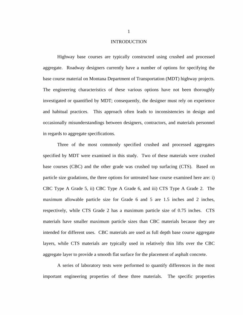
1

INTRODUCTION

Highway base courses are typically constructed using crushed and processed

aggregate. Roadway designers currently have a number of options for specifying the

base course material on Montana Department of Transportation (MDT) highway projects.

The engineering characteristics of these various options have not been thoroughly

investigated or quantified by MDT; consequently, the designer must rely on experience

and habitual practices. This approach often leads to inconsistencies in design and

occasionally misunderstandings between designers, contractors, and materials personnel

in regards to aggregate specifications.

Three of the most commonly specified crushed and processed aggregates

specified by MDT were examined in this study. Two of these materials were crushed

base courses (CBC) and the other grade was crushed top surfacing (CTS). Based on

particle size gradations, the three options for untreated base course examined here are: i)

CBC Type A Grade 5, ii) CBC Type A Grade 6, and iii) CTS Type A Grade 2. The

maximum allowable particle size for Grade 6 and 5 are 1.5 inches and 2 inches,

respectively, while CTS Grade 2 has a maximum particle size of 0.75 inches. CTS

materials have smaller maximum particle sizes than CBC materials because they are

intended for different uses. CBC materials are used as full depth base course aggregate

layers, while CTS materials are typically used in relatively thin lifts over the CBC

aggregate layer to provide a smooth flat surface for the placement of asphalt concrete.

A series of laboratory tests were performed to quantify differences in the most

important engineering properties of these three materials. The specific properties

2

examined in this study were: compaction, durability, strength, stiffness, and drainage

capacity. These properties were quantified by synthesizing and analyzing results from

the following laboratory tests:

Particle size gradation, Modified Proctor density, Relative density (maximum and minimum index densities), Specific gravity, Los Angeles abrasion/degradation, R-value, Direct shear, Permeability, and X-ray computed tomography.

Several of these tests were performed for basic classification purposes. The

equipment and procedures corresponding to each of these tests are considered

standardized. These basic classification and materials tests included particle size

gradation, modified Proctor density, relative density, specific gravity, and R-value tests.

Because these tests are standardized, there is little discussion of the equipment,

procedures, or interpretation of results in this report. The primary purpose of these tests

was for classification and general characterization of the materials.

Direct shear and permeability testing are standardized by both ASTM and

AASHTO, but not for the large particle sizes utilized in this study. Over-sized testing

apparatus were utilized in each case; consequently, more detailed discussions of testing

conditions and procedures are presented herein. These tests were a key aspect of this

study because strength and drainage are both vitally important to the performance of base

course aggregates and ultimately the pavement structure as a whole. Maximizing

strength and stiffness yields less rutting, smaller pavement deflections, and ultimately

3

less cracking of the pavement surface. Maximizing drainage yields less water in the

pavement structure; this reduces the damaging effects of water in the structural layers of

roadways. Maximization of both of these properties ultimately translates into longer

pavement service live.

X-ray computed tomography (CT) scanning was performed to attain pore size

distributions, which cannot be attained using more traditional methods for aggregate

materials with large pore sizes. Results from this testing were used to examine and

quantify the relationship between permeability and pore size distribution. X-ray CT is

not commonly used in soil analysis and there are no standardized testing procedures;

consequently, a thorough discussion of background information and test conditions are

presented.

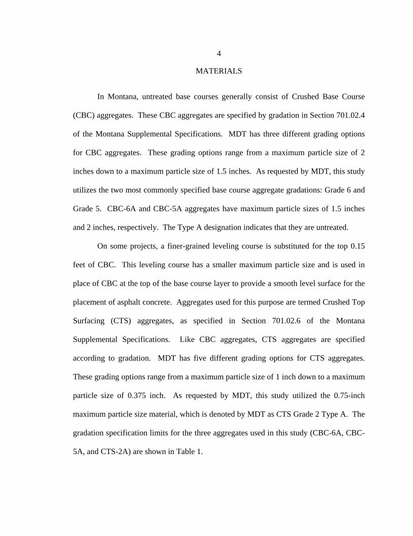
4

MATERIALS

In Montana, untreated base courses generally consist of Crushed Base Course

(CBC) aggregates. These CBC aggregates are specified by gradation in Section 701.02.4

of the Montana Supplemental Specifications. MDT has three different grading options

for CBC aggregates. These grading options range from a maximum particle size of 2

inches down to a maximum particle size of 1.5 inches. As requested by MDT, this study

utilizes the two most commonly specified base course aggregate gradations: Grade 6 and

Grade 5. CBC-6A and CBC-5A aggregates have maximum particle sizes of 1.5 inches

and 2 inches, respectively. The Type A designation indicates that they are untreated.

On some projects, a finer-grained leveling course is substituted for the top 0.15

feet of CBC. This leveling course has a smaller maximum particle size and is used in

place of CBC at the top of the base course layer to provide a smooth level surface for the

placement of asphalt concrete. Aggregates used for this purpose are termed Crushed Top

Surfacing (CTS) aggregates, as specified in Section 701.02.6 of the Montana

Supplemental Specifications. Like CBC aggregates, CTS aggregates are specified

according to gradation. MDT has five different grading options for CTS aggregates.

These grading options range from a maximum particle size of 1 inch down to a maximum

particle size of 0.375 inch. As requested by MDT, this study utilized the 0.75-inch

maximum particle size material, which is denoted by MDT as CTS Grade 2 Type A. The

gradation specification limits for the three aggregates used in this study (CBC-6A, CBC-

5A, and CTS-2A) are shown in Table 1.

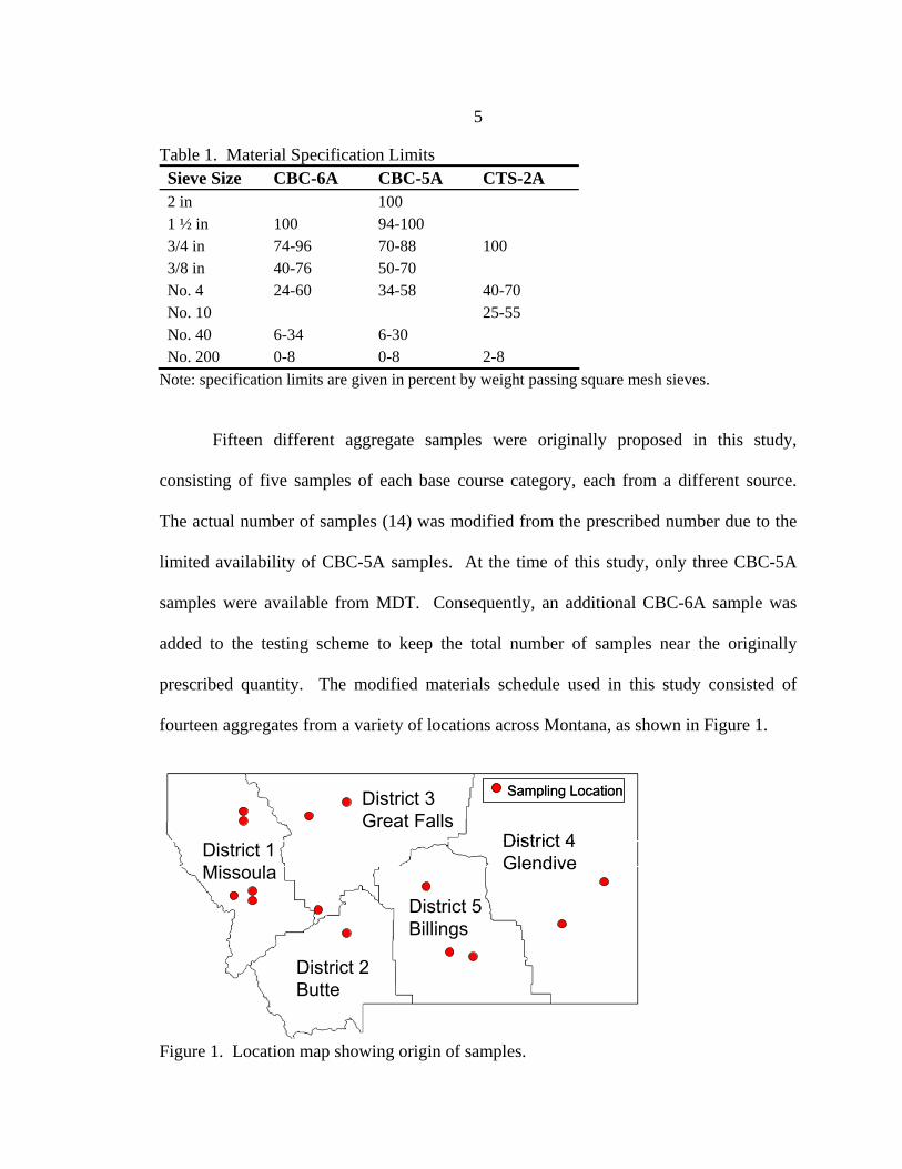
5

Table 1. Material Specification Limits Sieve Size CBC-6A CBC-5A CTS-2A 2 in 100 1 ½ in 100 94-100 3/4 in 74-96 70-88 100 3/8 in 40-76 50-70 No. 4 24-60 34-58 40-70 No. 10 25-55 No. 40 6-34 6-30 No. 200 0-8 0-8 2-8

Note: specification limits are given in percent by weight passing square mesh sieves.

Fifteen different aggregate samples were originally proposed in this study,

consisting of five samples of each base course category, each from a different source.

The actual number of samples (14) was modified from the prescribed number due to the

limited availability of CBC-5A samples. At the time of this study, only three CBC-5A

samples were available from MDT. Consequently, an additional CBC-6A sample was

added to the testing scheme to keep the total number of samples near the originally

prescribed quantity. The modified materials schedule used in this study consisted of

fourteen aggregates from a variety of locations across Montana, as shown in Figure 1.

Figure 1. Location map showing origin of samples.

District 1Missoula

District 2Butte

District 3Great Falls

District 4Glendive

District 5Billings

Sampling Location

District 1Missoula

District 2Butte


District 4Glendive

District 5Billings

District 1Missoula

District 2Butte


District 4Glendive

District 5Billings

Sampling LocationSampling Location

6

Table 2 shows the abbreviations for each material that will be used throughout

this report. Samples that are of different aggregate type yet labeled under the same town

name did not come from the same source pit, only from the same regional area. If each

aggregate type were sampled from the same pit in each town some variability would have

been eliminated. However, this would have required more samples to be tested

increasing time and cost. Additionally, the samples used here were the only ones

available at the time of sample collection.

Table 2. Materials Schedule Aggregate Type Abbreviation

Butte 6A-Butte Missoula 6A-Missoula Glendive 6A-Glendive Billings 6A-Billings Great Falls 6A-Great Falls

CBC-6A

Kalispell 6A-Kalispell Missoula 5A-Missoula Great Falls 5A-Great Falls CBC-5A Kalispell 5A-Kalispell Missoula 2A-Missoula Billings 2A-Billings Glendive 2A-Glendive Lewistown 2A-Lewistown

CTS-2A

Havre 2A-Havre

Photographs of 6A, 5A, and 2A aggregates are presented in Figure 2, Figure 3,

and Figure 4, respectively. All photos were taken at approximately the same scale, and a

graduated scale in inches is shown at the bottom of each photo. The following

7

differences in particle size and gradation between the CBC type aggregates and the CTS

type aggregates can be visually discerned by comparing Figure 2, Figure 3, and Figure 4.

All aggregates are relatively well graded.

2A aggregates have a smaller maximum particle size (0.75 inches), while the 6A and 5A aggregates have larger maximum particle sizes (1.5 and 2 inches).

The 5A aggregates appear to be slightly gap graded with some larger particles and an abundance of sand-size particles, while the 6A aggregates appear to have a better distribution and range of particle sizes.

Figure 2. Pictures of CBC-6A samples from a) Butte, b) Missoula, c) Glendive, d) Billings, e) Great Falls, and f) Kalispell.

Figure 3. Pictures of CBC-5A samples from a) Missoula, b) Great Falls, and c) Kalispell.

d)

a) b) c)

e) f)

a) b) c)

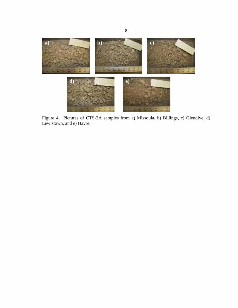
8

Figure 4. Pictures of CTS-2A samples from a) Missoula, b) Billings, c) Glendive, d) Lewistown, and e) Havre.

a) b) c)

d) e)

9

AGGREGATE MATERIALS TESTING

Aggregate materials testing includes any soils testing that would normally be

performed on a base course aggregate on a MDT roadway construction project. This

chapter begins with a description of the statistical testing that was used to evaluate results

where averages for each aggregate type were examined. Soils tests that could be termed

“index tests” are then presented (particle size distribution, modified Proctor compaction,

relative density, and specific gravity). The Los Angeles abrasion and R-value tests are

also commonly performed by the MDT materials laboratory for many roadway

construction projects.

Statistical Evaluation of Results

The primary focus of this project is to determine relative differences in important

engineering properties between three different aggregate types. Statistical analyses of

average values based on aggregate type were conducted using the two sample t-test to

determine if apparent trends in measured laboratory test results represent true differences

between aggregate types. The following statistical symbols are used throughout this

report:

µ = average (also known as the mean) σ = standard deviation COV = coefficient of variation (σ/µ)

The two sample t-test is a statistical test used to determine if the averages of two

data sets are statistically different based on a mathematical evaluation of data scatter. It

can further be used to determine the relationship between the two averages; i.e., whether

10

one average is greater than, less than, or equal to the other. Three separate comparisons

are required to determine the relationship between each set of test results (i.e., 6A versus

5A, 6A versus 2A, and 5A versus 2A).

The output of interest from this statistical test is the p-value parameter, which

ranges from 0 to 1 based on the methodology used in this study. p-values from the two

sample t-test can be used to indicate how two average values compare to each other

taking into account data scatter and the number of data points. In this investigation,

results from the two sample t-test were interpreted as follows:

p-values between 0 and 0.15 indicated that one average was statistically less than another average;

p-values between 0.85 and 1.0 indicated that one average is statistically greater than another average; and

p-values between 0.15 and 0.85 indicated the two averages being compared are not statistically different, which is denoted here with an equal sign (see Figure 5).

This latter outcome may be because the averages were truly the same, or that the

standard deviations are relatively large compared to the difference between the averages.

In either case, no statistically significant differences can be discerned between the two

averages. The two sample t-test does not inherently include cut-off p-values for

evaluating the relationship between data sets; rather appropriate cutoff values must be

selected by the user. The cut-off p-values of 0.15 and 0.85 were selected by the

researchers in this study using judgment based on the relatively large variability that is

typically observed in geotechnical test data.

11

Figure 5. p-value ranges utilized in this study for the two sample t-test.

Particle Size Distribution

Grain size analyses were completed on each of the 14 samples in general

accordance with AASHTO Test Method T311 and MDT Test Method MT202. Particle

size distributions were compared to MDT specified upper and lower gradation limits,

which are described in Sections 701.02.4 and 701.02.6 of the Montana Supplemental

Specifications. Screen sizes used for gradation analyses were selected based on MDT

specifications, as shown in Table 3. Figure 6 shows a comparison plot of the

specification limits for the three aggregate types compared in this study.

Table 3. Sieve Sizes Utilized in this Study Sieve Opening

(in) (mm) Standard Sieve Size

2 50 - 1.5 37.5 - 1 25 - 0.75 19 - 0.5 12.5 - 0.375 9.5 - 0.187 4.75 No. 4 0.079 2 No. 10 0.017 0.425 No. 40 0.003 0.075 No. 200

A dash indicates that a standard sieve size does not exist for this sieve opening size.

12

Figure 6. MDT specification limits for CBC-5A, CBC-6A, and CTS-2A.

Grain size analyses were performed by two separate labs. One set of analyses

was performed at the Montana State University (MSU) geotechnical laboratories, and

another set was completed by MDT. MSU grain size distributions are shown in Figure 7

through Figure 9, and copies of MDT grain size distributions are provided in Appendix

A. Gradation plots compare favorably for the two sets of analyses, with only one notable

difference; the MSU gradations show less fine material than the MDT grain size

distributions. One explanation of the discrepancy between the results is that the MDT lab

performed a wash test on the minus No. 4 size particles, while the MSU lab did not.

Wash testing was not performed at the MSU lab because these materials contained

relatively few fines and it was thought that washing would have a relatively minor impact

on the results. The slight differences in results could also partially be attributed to

Particle Size (mm)

0.010.1110100

Perc

ent P

assi

ng

0

20

40

60

80

100

5A Specification Limits 6A Specification Limits2A Specification Limits

50 mm = 1.97 in

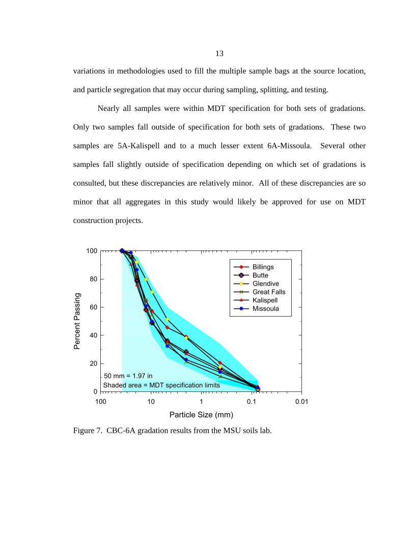
13

variations in methodologies used to fill the multiple sample bags at the source location,

and particle segregation that may occur during sampling, splitting, and testing.

Nearly all samples were within MDT specification for both sets of gradations.

Only two samples fall outside of specification for both sets of gradations. These two

samples are 5A-Kalispell and to a much lesser extent 6A-Missoula. Several other

samples fall slightly outside of specification depending on which set of gradations is

consulted, but these discrepancies are relatively minor. All of these discrepancies are so

minor that all aggregates in this study would likely be approved for use on MDT

construction projects.

Figure 7. CBC-6A gradation results from the MSU soils lab.

Particle Size (mm)

0.010.1110100

Perc

ent P

assi

ng

0

20

40

60

80

100

Billings Butte Glendive Great Falls Kalispell Missoula

Shaded area = MDT specification limits50 mm = 1.97 in

14

Figure 8. CBC-5A gradation results from the MSU soils lab.

Figure 9. CTS-2A gradation results from MSU soils lab.

Particle Size (mm)

0.010.1110100

Perc

ent P

assi

ng

0

20

40

60

80

100

Great Falls Kalispell Missoula


Particle size (mm)0.010.1110100

Perc

ent P

assi

ng

0

20

40

60

80

100

Missoula Glendive Havre Lewistown Lewistown (re-test) Billings


15

Modified Proctor Compaction

Modified Proctor testing was conducted in general accordance with AASHTO

Test Method T180 and MDT Test Method MT230. Because the 2A aggregates had a

maximum particle size of 0.75 inches, no screening of oversize particles was necessary

with the 6-inch-diameter Proctor mold. Material greater than the 0.75-inch sieve was

screened off for testing of the 6A and 5A materials and replaced with an equal weight of

material between the No. 4 and 0.75-inch sieve sizes, as specified in MT230. When

testing the 6A and 5A materials, several difficulties were encountered in obtaining results

that were accurate and repeatable enough for research purposes. These difficulties

included excessive amounts of water and fines washing out of the bottom of the Proctor

mold, excessive movement of particles when the hammer was applied to the sample, and

variations in measured densities depending on the approach used to level-off the top

surface of the test specimen. The combined effect of these factors led to wide variation

in the results. This variation is generally attributed to the open graded nature of the 6A

and 5A aggregates.

ASTM Test Method D2049 specifies that relative index density testing is

appropriate for materials with less than 12% passing the No. 200 sieve. In addition, as

described in AASHTO Test Methods T99 and T180, the Proctor test is not necessarily

applicable for use on cohesionless soils. All aggregate samples evaluated in this study

have less than 12% fines and are cohesionless. Consequently, densities obtained from

maximum and minimum index density testing (ASTM D4253 and ASTM D4254) were

16

used in place of Proctor densities for evaluating relative densities of prepared samples in

this study.

Accurate modified Proctor data was gathered for the 2A samples, even though

testing was not completed on 6A or 5A samples. Modified Proctor maximum dry

densities (for the 2A samples) were similar in magnitude to dry densities determined

using the saturated maximum index density method, as shown in Figure 10. Density

measurements are provided in terms of void ratio (e) in Figure 10, which can be related to

dry unit weight (γd) using Equation (1), as follows:

e

G wsd +

=1

γγ (1)

where, Gs = specific gravity, γw = unit weight of water, and e = void ratio.

Figure 10. CTS-2A modified Proctor and maximum index density comparison.

0.0

0.1

0.2

0.3

0.4

0.5

0.6

0.7

0.8

0.9

1.0

Source Location

Voi

d R

atio

( e)

Modified Proctor density

Maximum and minimum index densities

Bill

ings

Gle

ndiv

e

Lew

isto

wn

Hav

re

Mis

soul

a

17

This indicates that either method (saturated maximum index density or modified

Proctor) for determining maximum density would be acceptable for the 2A aggregates.

For consistency, maximum dry densities obtained using the maximum index density test

were used in this study for all three aggregate types. It is expected that if accurate

Proctor densities could be obtained for 5A and 6A aggregates, they would likely also

correspond to maximum dry densities measured using the maximum index density test

because these aggregates are similar in structure to 2A aggregates.

Relative Density

Relative density testing was conducted in general accordance with ASTM Test

Method D4253 (Maximum Index Density and Unit Weight of Soils Using a Vibratory

Table) and ASTM Test Method D4254 (Minimum Index Density and Unit Weight of

Soils and Calculation of Relative Density). ASTM D4253 provides the option of

conducting either dry or saturated testing. It was observed in this study that saturated

testing yielded significantly lower minimum void ratios (higher maximum densities) than

dry testing. Consequently, all maximum index density results reported herein are based

on tests performed under saturated conditions. The size of the mold used for testing was

governed by the ASTM specification, which is based on the maximum particle size of the

sample. The 5A and 6A samples were tested in the 10-inch-diameter (volume = 0.500

ft3) mold, while 2A samples were tested in the 6-inch-diameter (volume = 0.100 ft3)

mold. Relative density can be calculated in terms of either void ratio or dry density as:

⎥⎦

⎤⎢⎣

⎡

⎥⎥⎦

⎤

⎢⎢⎣

⎡

−

−=

−−

=d

d

dd

ddr ee

eeDρ

ρρρ

ρρ (max)

(min)(max)

(min)

minmax

max (2)

18

where, Dr = relative density, emax = maximum void ratio, emin = minimum void ratio, e =

in-situ void ratio, ρd = in-situ density, ρd(max) = maximum index density, and ρd(min) =

minimum index density.

Maximum and minimum index density results are summarized in Figure 11 in

terms of void ratio. This figure shows maximum and minimum void ratios, as well as the

associated void ratio spread (emax−emin) for each aggregate. The majority of specimens

compacted to an emin between 0.20 and 0.25, with three exceptions. The 5A-Kalispell

sample had the lowest emin value (0.17), while the 6A-Missoula and 6A-Glendive samples

were on the high end with emin values of 0.29 and 0.27, respectively.

Figure 11. Maximum and minimum index density test results.

0.00.10.20.30.40.50.60.70.80.91.0

Source Location

Voi

d R

atio

(e)

Billi

ngs

Gle

ndiv

e

Gre

at F

alls

Kal

ispe

ll

Mis

soul

a

But

te

Mis

soul

a

Gre

at F

alls

Kal

ispe

ll

Billi

ngs

Gle

ndiv

e

Lew

isto

wn

Hav

re

Mis

soul

a

CBC-6A CBC-5A CTS-2A

19

Specific Gravity

Specific gravity (Gs) tests were conducted on the 14 aggregate samples in general

accordance with AASHTO Test Method T100 (Specific Gravity of Soils) and AASHTO

Test Method T85 (Specific Gravity and Absorption of Coarse Aggregate). Specific

gravity was determined by taking a weighted average from the fine and coarse fractions

of each soil sample. Aggregate type is not expected to have any relation to Gs.

Additionally, different aggregate types that have the same location label may not have

corresponding Gs values because samples did not necessarily come from the same pit

only the same region. Values ranging from 2.66 to 2.76 were obtained for the samples

tested in this study; well within the typical range reported for these material types (Das

2002). Specific gravity results are summarized in Table 4.

Table 4. Specific Gravity Results Aggregate Type Specific Gravity

Great Falls 2.73 Billings 2.71 Glendive 2.71 Missoula 2.72 Butte 2.68

CBC-6A

Kalispell 2.69 Great Falls 2.73 Missoula 2.70 CBC-5A Kalispell 2.69 Havre 2.66 Glendive 2.76 Missoula 2.76 Lewistown 2.71

CTS-2A

Billings 2.72

20

Los Angeles Abrasion

Los Angeles (LA) abrasion tests were conducted in general accordance with

AASHTO Test Method T96 and MDT Test Method MT209 (Resistance to Degradation

of Small-Size Coarse Aggregate by Abrasion and Impact in the Los Angeles Machine).

LA abrasion tests are used to quantify the relative durability of aggregates. Aggregate

durability is thought to depend on mineralogy so no relation to aggregate type was

expected. Results from LA abrasion testing are summarized in Table 5. The 2A-Havre

and 5A-Missoula samples fell outside of the MDT specification limit of 40 percent loss,

with LA abrasion loss percentages of 48.2 and 61.9, respectively. All other samples fell

within the MDT specification limit for durability.

The loss value for the 2A-Havre sample is about 8 percent greater than the

specification limit, and the loss for 5A-Missoula is about 22 percent greater than the

limit. It was noted during direct shear testing that the larger particles of the 5A-Missoula

sample contained conglomerations of smaller particles that broke apart under load. It is

likely that these weaker particles contributed to the high loss obtained using the LA

impact device.

21

Table 5. Los Angeles Abrasion Results Aggregate Type Percent Loss

Great Falls 27.3 Billings 23.5 Glendive 22.3 Missoula 15.3 Butte 19.0

CBC-6A

Kalispell 15.5 Great Falls 19.0 Missoula 61.9 CBC-5A Kalispell 13.2 Havre 48.2 Glendive 15.3 Missoula 13.1 Lewistown 24.1

CTS-2A

Billings 16.9

Resistance Value

The Resistance R-value and Expansion Pressure of Compacted Soils test

(commonly referred to as the R-value test) is used by MDT to evaluate the strength and

stability of subgrade and base materials. The test is standardized by AASHTO Test

Method T190 and ASTM Test Method D2844. Testing was completed by MDT at their

Helena materials testing lab. R-value test output is a number ranging from 0 to 100, with

0 representing viscous liquid slurry with no shear resistance, and 100 representing a rigid

solid. The R-value test is conducted using a stabilometer, which is shown schematically

in Figure 12. Testing involves applying a constant vertical pressure to the sample and

measuring the corresponding increase in horizontal (fluid) pressure. The R-value is

calculated based on the ratio of vertical pressure applied to the amount of fluid pressure

measured.

22

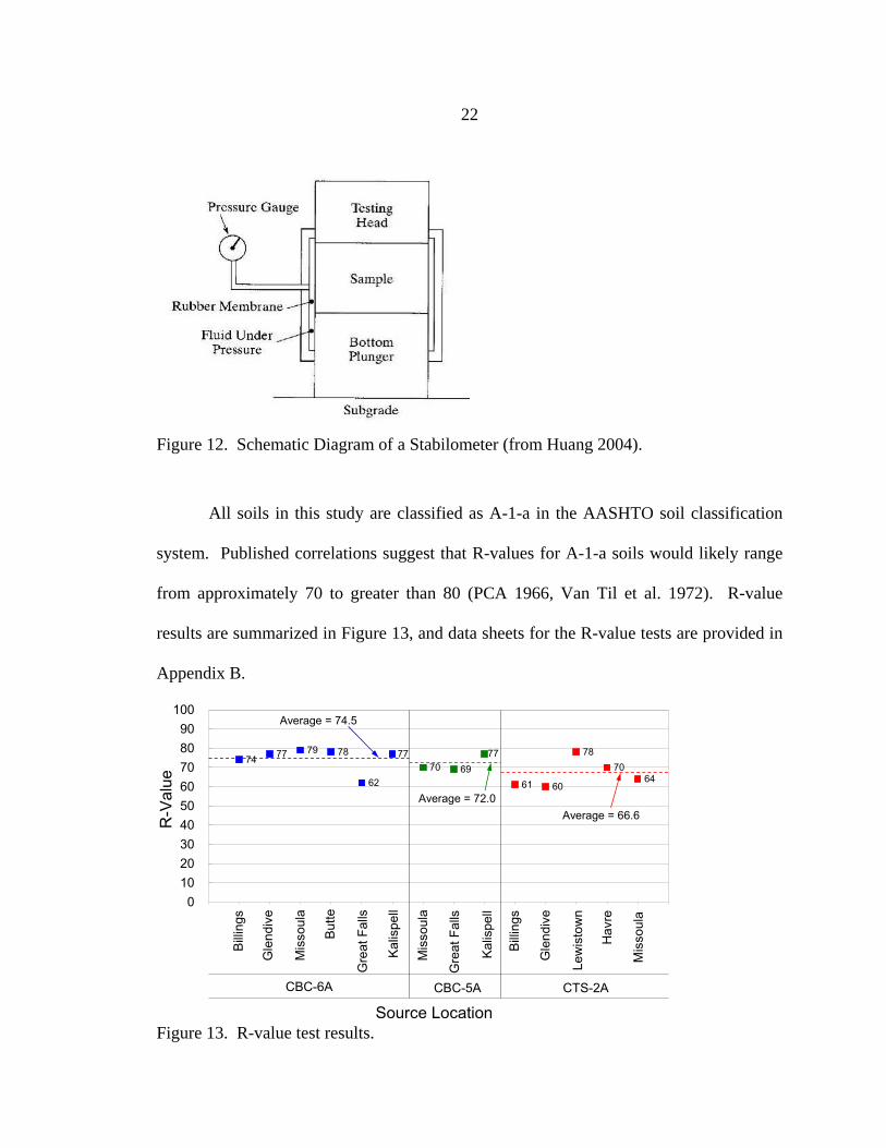
Figure 12. Schematic Diagram of a Stabilometer (from Huang 2004).

All soils in this study are classified as A-1-a in the AASHTO soil classification

system. Published correlations suggest that R-values for A-1-a soils would likely range

from approximately 70 to greater than 80 (PCA 1966, Van Til et al. 1972). R-value

results are summarized in Figure 13, and data sheets for the R-value tests are provided in

Appendix B.

Figure 13. R-value test results.

74 77 79 7870 69

61 60

7870

64

77 77

62

0102030405060708090

100

Source Location

R-V

alue

Bill

ings

Gle

ndiv

e

Gre

at F

alls

Kal

ispe

ll

Mis

soul

a

But

te

Mis

soul

a

Gre

at F

alls

Kal

ispe

ll

Bill

ings

Gle

ndiv

e

Lew

isto

wn

Hav

re

Mis

soul

a


Average = 74.5

Average = 72.0Average = 66.6

23

As shown in Figure 13, slight differences in average R-values were observed

between the different aggregate types. A series of two sample t-tests were performed to

determine if differences in the average values were statistically significant. Results from

this statistical evaluation are shown in Table 6. Based on the statistical testing, the

average 2A R-value (66.6) was less than both the average 6A R-value (74.5) and the

average 5A R-value (72.0). There is no statistically significant difference between the

average 6A and average 5A R-values. From a practical viewpoint, the relative

differences are not significant based on the accuracy of the test.

Table 6. Average R-value Statistical Evaluation Relationship p-value

6A = 5A µ=74.5 µ=72.0

0.740

6A > 2A µ=74.5 µ=66.6

0.950

5A > 2A µ=72.0 µ=66.6 0.873

24

DIRECT SHEAR

Direct shear testing was performed to supplement R-value testing by providing

another means of quantifying shear strength parameters of the aggregate samples. Tests

were performed in general accordance with AASHTO Test Method T236. A 12-inch by

12-inch Brainard-Kilman direct shear testing apparatus was used to accommodate the

large maximum particle size of the aggregate samples. Shear resistance was measured

using an S-type load cell and lateral displacement was measured using a linear variable

displacement transducer (LVDT). Figure 14 shows some of the main components of the

direct shear device.

Background

The direct shear test is used to obtain average macro strength properties of a soil

sample by measuring the load required to induce shear failure along a predetermined

plane. A flat shear failure plane is commonly assumed because there is no practical way

to measure the shape of the actual failure plane in a direct shear test, which has been

shown by Atkinson and Bransby (1978) to be elliptical. Localized strains in the sample

are not measured, and high stress concentrations near the sample boundaries can lead to

non-uniform stress conditions (Holtz and Kovacs 1981). Consequently, the average

strain is calculated from displacement, and the average stress is calculated from the load.

25

Figure 14. Direct shear testing apparatus a) mold halves, b) mold placed in load frame with a crane, c) vibratory compactor, and d) assembled mold halves with air bladder and cover plate attached to top.

The direct shear machine is a reasonable, practical device for quantifying stresses

that cause failure on a specific (horizontal) failure plane (Atkinson and Bransby 1978).

This test was selected as a method for quantifying strength and stiffness because it

provides a repeatable approach for quantifying relative differences between the aggregate

types examined in this study. The test was also selected because it is relatively easy to

perform compared to the triaxial test; especially for aggregates containing large particle

sizes, like those utilized in this study.

a) b)

c)

d)

26

Testing Conditions

Testing conditions are presented here to document the details of equipment setup

and sample preparation that are not specified for the over-size samples utilized in this

study.

Apparatus and Sample Preparation

Soil was placed into the shear box in 1.3-inch compacted lifts. Compaction was

performed at 4% moisture using a 57-pound pneumatic vibratory compactor with a 100

in2 contact area (Figure 14c). Normal stress (pressure) was applied to the sample using a

pressurized rubber air bladder, which was located on the inside of the shear box lid

(Figure 14d). The samples were sheared at a constant rate of 0.05 in/min to a maximum

horizontal displacement of 3.8 inches. The horizontal displacement rate was slow enough

to ensure full drainage (effective stress conditions).

Compacted Density of Samples

In the field, large vibratory drum compactors pass over a material multiple times

to impart weight and vibration to the underlying geomaterials. This process was

simulated in the laboratory using a weighted vibratory plate. Vibration and impact

compaction energy were applied until observable particle movement ceased, which

generally occurred after approximately 1 minute of compaction for each soil layer. This

method of compaction provided high densities with minimal compaction non-

uniformities. All samples were compacted using an initial water content of 4% to help

minimize particle segregation and achieve high densities.

27

The dry density of each direct shear sample was determined using mass-volume

relationships after each sample was compacted into the direct shear mold. Relative

density (Dr) was calculated for each compacted sample using Equation (2). There is

some variation in Dr between aggregate types because of the differences in particle

gradation, particle shape, and maximum particle size. Overall, good repeatability was

achieved using this method of compaction, as evidenced by the relatively small spread of

compacted void ratios, as shown by the dashed symbols in Figure 15.

Figure 15. Void ratio (e) for each direct shear test compared to emax and emin.

Results

Several parameters were obtained from direct shear testing including initial

stiffness (ki), ultimate secant stiffness (ku), and ultimate strength (σu). Mohr-Coulomb

failure envelopes were determined from the ultimate strength of each material at different

0.00.10.20.30.40.50.60.70.80.91.0

Source Location

Voi

d R

atio

(e)

Direct shear test

Maximum and minimumindex densities

Billi

ngs

Gle

ndiv

e

Gre

at F

alls

Kal

ispe

ll

Mis

soul

a

But

te

Mis

soul

a

Gre

at F

alls

Kal

ispe

ll

Billin

gs

Gle

ndiv

e

Lew

isto

wn

Hav

re

Mis

soul

a


* If less than 3 void ratios are displayed for each sample, some of them overlap.

28

normal stresses. Values of ki reported here are defined as the slope of the linear elastic

portion of the stress-displacement curve, which occurs at low displacements. Ultimate

secant stiffness is defined as the slope of a line drawn from the origin to the shear stress

at 8% strain, where the strain is averaged over the entire length of the sample. Percent

strain in this context is thus defined as the measured displacement divided by sample

width. σu was determined at 8% strain or the peak stress, whichever occurred first. An

example illustrating how these values were determined for the 6A-Missoula, 10 psi

sample, is shown in Figure 16. Shear stress versus horizontal displacement plots for all

three normal stresses are provided in Appendix C for each material.

Figure 16. Example of strength parameter (ki, ku, and σu) determination.

0

500

1,000

1,500

2,000

2,500

3,000

3,500

4,000

4,500

5,000

0.0 0.5 1.0 1.5 2.0 2.5 3.0Displacement (in)

Load

(lb)

6A Missoula, 10 psi

Displacement = 0.96 in (εavg = 8%)

Secant Stiffness (k u ) = 3,337 lb/in

σ u

Initial Stiffness (k i ) = 25,680 lb/in

29

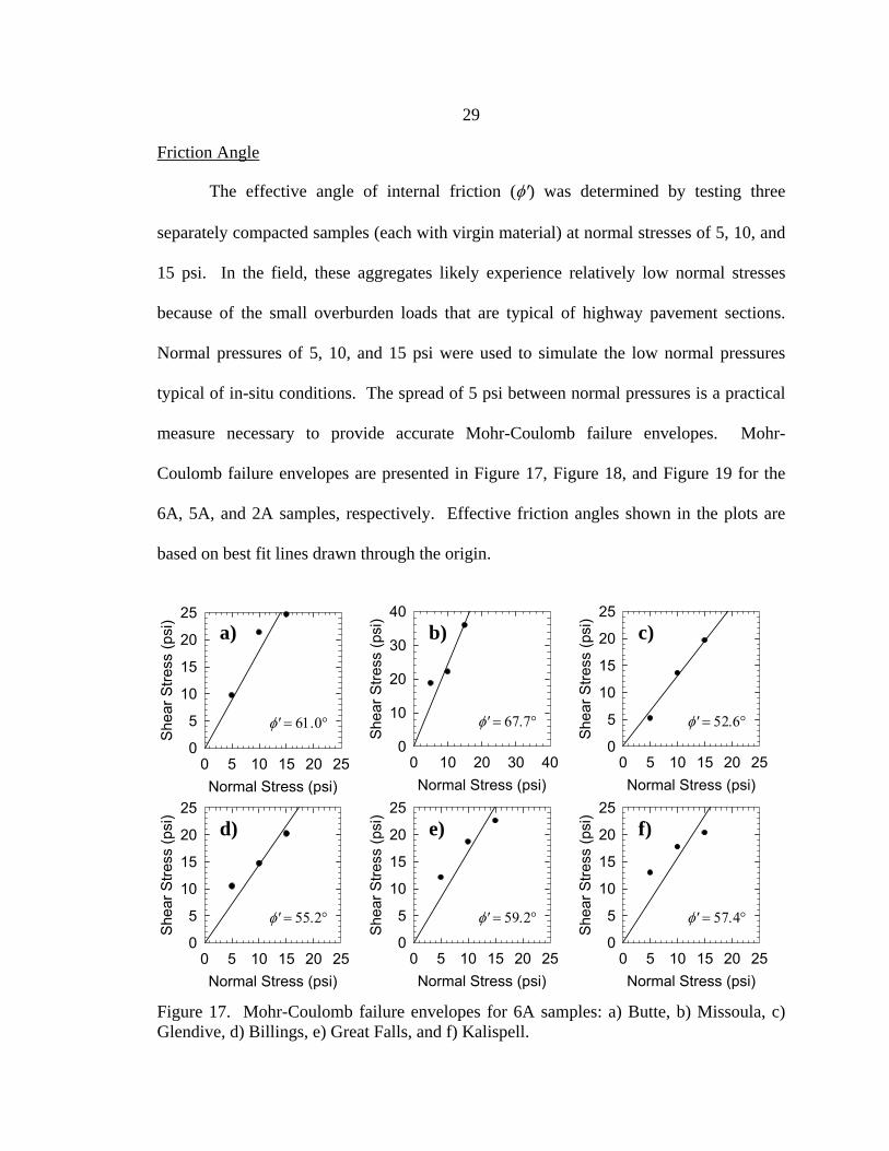
Friction Angle

The effective angle of internal friction (φ′) was determined by testing three

separately compacted samples (each with virgin material) at normal stresses of 5, 10, and

15 psi. In the field, these aggregates likely experience relatively low normal stresses

because of the small overburden loads that are typical of highway pavement sections.

Normal pressures of 5, 10, and 15 psi were used to simulate the low normal pressures

typical of in-situ conditions. The spread of 5 psi between normal pressures is a practical

measure necessary to provide accurate Mohr-Coulomb failure envelopes. Mohr-

Coulomb failure envelopes are presented in Figure 17, Figure 18, and Figure 19 for the

6A, 5A, and 2A samples, respectively. Effective friction angles shown in the plots are

based on best fit lines drawn through the origin.

Figure 17. Mohr-Coulomb failure envelopes for 6A samples: a) Butte, b) Missoula, c) Glendive, d) Billings, e) Great Falls, and f) Kalispell.

Normal Stress (psi)0 5 10 15 20 25

She

ar S

tress

(psi

)

0

5

10

15

20

25

φ' = 61.0°

Normal Stress (psi)0 10 20 30 40

Shea

r Stre

ss (p

si)

0

10

20

30

40

φ' = 67.7°


Shea

r Stre

ss (p

si)

0

5

10

15

20

25

φ' = 52.6°


She

ar S

tress

(psi

)

0

5

10

15

20

25

φ' = 55.2°


Shea

r Stre

ss (p

si)

0

5

10

15

20

25

φ' = 59.2°


Shea

r Stre

ss (p

si)

0

5

10

15

20

25

φ' = 57.4°

a) b) c)

d) e) f)

30

Figure 18. Mohr-Coulomb failure envelopes for 5A samples: a) Missoula, b) Great Falls, and c) Kalispell.

Figure 19. Mohr-Coulomb failure envelopes for 2A samples: a) Missoula, b) Billings, c) Glendive, d) Lewistown, and e) Havre.

Measured φ′ values were in the range of 49° to 68°, which represents a relatively

large spread. Figure 20 provides a direct comparison of φ′ values for the three aggregate

types. A series of two sample t-tests were performed on the average φ′ values to

Normal Stress (psi)0 5 10 15 20 25 30

Shea

r Stre

ss (p

si)

05

1015202530

φ' = 60.2°


She

ar S

tress

(psi

)

0

5

10

15

20

25

φ' = 54.1°


She

ar S

tress

(psi

)

0

5

10

15

20

25

φ' = 54.7°

a) b) c)


She

ar S

tress

(psi

)0

5

10

15

20

25

φ' = 56.6°


She

ar S

tress

(psi

)

0

5

10

15

20

25

φ' = 56.9°


She

ar S

tress

(psi

)

0

5

10

15

20

25

φ' = 52.2°

d) e)


She

ar S

tress

(psi

)

0

5

10

15

20

25

φ' = 60.6°


She

ar S

tress

(psi

)

0

5

10

15

20

25

φ' = 49.3°

a) b) c)

31

determine the statistical significance of the scatter or spread in results. The results of this

statistical evaluation are summarized in Table 7, which indicates that the average 6A

effective friction angle (58.8°) is larger than the average 2A friction angle (55.1°). When

the spread of data is taken into account, there is not a significant difference in the φ′

values between the 6A and 5A materials or between the 5A and 2A materials.

Figure 20. Internal friction angles (φ′) for each aggregate.

Table 7. Average Internal Friction Angle (φ′)Statistical Evaluation Relationship p-value

6A = 5A µ=58.8 µ=56.3

0.791

6A > 2A µ=58.8 µ=55.1

0.882

5A = 2A µ=56.3 µ=55.1 0.660

55.2

52.6

67.7

61.0 60.2

49.3

56.6

52.2

56.9

60.659.2

54.1 54.7

57.4

40

45

50

55

60

65

70

Source Location

Inte

rnal

Fric

tion

Ang

le (d

eg)

Billin

gs

Gle

ndiv

e

Gre

at F

alls

Kal

ispe

ll

Mis

soul

a

Butte

Mis

soul

a

Gre

at F

alls

Kal

ispe

ll

Billin

gs

Gle

ndiv

e

Lew

isto

wn

Hav

re

Mis

soul

a


Average = 58.8

Average = 56.3 Average = 55.1

32

Initial Stiffness

Failure of roadway materials is generally defined by relatively small

deformations, which are related to the initial portion of the stress-displacement curve.

The initial stiffness, ki, is defined as the slope of the stress-displacement curve at low

displacements, where the curve is relatively linear, as shown in Figure 16.

Values of ki for all of the samples tested are compared in Figure 21. These values

generally ranged from 10,000 lb/in to 30,000 lb/in. As expected, most aggregates

exhibited increasing ki with increasing normal stress. There were some minor exceptions

to this trend, which may be attributed to small variations in the test pressures and

variations in sample collection methodology, compaction non-uniformities, and minor

particle segregation during sampling and sample preparation.

Figure 21. Initial stiffness (ki) results.

0

10,000

20,000

30,000

40,000

50,000

60,000

Source Location

Stiff

ness

(lb/

in)

5 psi

10 psi

15 psi

Billi

ngs

Gle

ndiv

e

Gre

at F

alls

Kal

ispe

ll

Mis

soul

a

But

te

Mis

soul

a

Gre

at F

alls

Kal

ispe

ll

Billi

ngs

Gle

ndiv

e

Lew

isto

wn

Hav

re

Mis

soul

a


Average = 22,100

Average = 17,300 Average = 17,100

33

A series of two sample t-tests were performed to determine if the apparent trends

in average ki values were statistically significant. The results of the statistical evaluation

are summarized in Table 8. The average ki of the 6A aggregate type (22,100 lb/in) is

statistically greater than the average ki of the 2A aggregate type (17,100 lb/in) and the 5A

aggregate type (17,300 lb/in). There is no significant difference between the average ki

of the 5A and 2A aggregate types.

Table 8. Average Initial Stiffness (ki) Statistical Evaluation Relationship p-value

6A > 5A µ=22.1 µ=17.3

0.931

6A > 2A µ=22.1 µ=17.1

0.953

5A = 2A µ=17.3 µ=17.1 0.552

Secant Stiffness

Ultimate secant stiffness (ku) values were determined for each aggregate to

evaluate the soil behavioral characteristics at large strains. Ultimate secant stiffness is

defined here as the slope of a line drawn from the origin to the shear stress at 8% strain

on a shear stress-displacement curve, as shown in Figure 16. Ultimate secant stiffness

may not be as relevant as ki because roadway base course aggregates would likely not

experience 8% strain during normal service. However, ku is an additional, meaningful

parameter that can be used for quantifying strength and stiffness differences between

aggregate types.

34

As shown in Figure 22, ku values generally ranged from 1,000 lb/in to 3,500 lb/in.

All aggregates exhibited increasing ku values with increasing normal stresses. The 6A-

Missoula sample exhibited significantly higher secant stiffness than all of the other

samples. A series of two sample t-tests were performed to compare average ku values

based on aggregate type. Results of this statistical evaluation are presented in Table 9.

Figure 22. Secant stiffness (ku) results.

Table 9. Average Secant Stiffness (ku) Statistical Evaluation Relationship p-value

6A > 5A µ=2.44 µ=2.20

0.878

6A > 2A µ=2.44 µ=2.16

0.934

5A = 2A µ=2.20 µ=2.16 0.538

0

1,000

2,000

3,000

4,000

5,000

6,000

Source Location

Stiff

ness

(lb/

in)

5 psi

10 psi

15 psi


Billi

ngs

Gle

ndiv

e

Gre

at F

alls

Kal

ispe

ll

Mis

soul

a

But

te

Mis

soul

a

Gre

at F

alls

Kal

ispe

ll

Billi

ngs

Gle

ndiv

e

Lew

isto

wn

Hav

re

Mis

soul

a

Average = 2,440 Average = 2,200 Average = 2,160

35

The average ku of the 6A aggregate type (2,440 lb/in) is greater than the average

of the 2A aggregate type (2,160 lb/in) and the 5A aggregate type (2,200 lb/in). There is

no significant difference between the average ku of the 5A and 2A aggregates. This

indicates that at relatively large displacements, these aggregates all exhibit relatively

similar stress-displacement behavior, with the 6A aggregate type exhibiting only a small

potential advantage over the other aggregates. Trends observed in the ku results are

similar to the ki results.

Summary

Sample preparation techniques and testing procedures were adapted for an over-

sized 12-inch by 12-inch direct shear box. Results for all three parameters determined in

direct shear testing are summarized in Table 10. These results indicate that, in general,

the 6A aggregates were the strongest and stiffest examined in this study, followed by the

5A, and then the 2A aggregates.

Table 10. Summary of Direct Shear Results ki ku φ′

6A > 5A 6A > 5A 6A = 5A 6A > 2A 6A > 2A 6A > 2A 5A = 2A 5A = 2A 5A = 2A

36

PERMEABILITY

Drainage capacity was quantified through saturated constant head hydraulic

conductivity (permeability) testing. Permeability (k) tests were performed in general

accordance with ASTM Test Method D2434 and AASHTO Test Method T215

(Permeability of Granular Soils - Constant Head). Constant head testing was utilized (as

opposed to falling head) to limit the amount of hydraulic head applied to the samples thus

ensuring laminar flow conditions. Darcy’s Law was used to compute k, as follows:

tHAQLk = (3)

where, k = permeability, Q = volume of water passed through the specimen, L = length of

the specimen, t = elapsed time corresponding to Q, H = total head across the specimen,

and A = cross sectional area of the specimen perpendicular to the flow direction.

Testing the least permeable layer of a soil sample in the laboratory is a commonly

accepted method for quantifying the speed with which a fluid will pass through porous

media. Permeability is a highly variable soil property that can vary significantly with

small variations in compaction and gradation. To minimize testing errors, average k

values were obtained for each sample by conducting three separate tests, using virgin

aggregate each time. Experimental results were compared to empirical estimation

equations and published typical ranges to verify laboratory test results, and to evaluate

the prediction methods themselves to determine if any performed well for the aggregates

in this study.

37

Testing Conditions

Testing conditions are presented here to document the details of equipment setup,

sample preparation, and testing procedures that are not specified for the over-size

samples utilized in this study.

Apparatus

A custom-built large-diameter permeameter was utilized for this testing. The

permeameter specimen mold has a diameter of 10 inches and an approximate height of 10

inches. The permeameter utilizes a unique Mariotte tube and integral upper reservoir

arrangement to maintain constant pressure head and complete saturation of the soil

sample and testing apparatus throughout the experiment. A photograph and schematic

diagram of the permeameter are shown in Figure 23.

Figure 23. Photograph and schematic diagram of permeameter setup.

Upper reservoir

Mariotte (bubble) tube

Coupling & Support plate

Specimen mold

Coupling & Support plate

Drainage port

Fill port

Screens

38

There are several notable improvements in this custom-built device over a

traditional constant head permeability testing apparatus. The apparatus used in this study

completely submerges the specimen in the tail water tank, which ensures the specimen

remains saturated throughout the test. There is no head loss between the head water tank

and specimen because there are no tubes, valves, or fittings between the headwater and

specimen. Only a screen and support plate separates the supply water from the specimen.

The upper reservoir is used to supply water to the sample and can be precisely measured

using a manometer, which eliminates the need to collect and measure the tail water.

Additionally, the use of a Mariotte tube to maintain constant head eliminates the waste of

overflow head water, which is inherent in traditional permeameter devices.

The specimen support plates are shown in Figure 24. The support plates consist

of 0.25 inch thick galvanized steel plates that have 0.25 inch holes throughout to permit

the unrestricted flow of water. Two square mesh screens, oriented at 45° relative to each

other, were placed between the sample and the support plates to reduce the washing of

finer particles out of the specimen during testing. The screens were placed at 45° relative

to each other to further reduce the opening size of the sieves, thereby reducing the

movement of fines.

A 0.125-inch thick soft neoprene rubber liner with 450 psi tensile strength and

10A durometer hardness was attached to the inside of the specimen mold with silicone

adhesive to reduce edge effects, as suggested by Thornton and Toh (1995). The liner was

installed to alleviate high stress concentrations that may occur at the contact points of the

larger particles on the smooth rigid interior wall of the mold, and to maintain a more

uniform and representative distribution of particles near the sample edges. The liner was

39

used for all tests performed in this study. Any effect imparted on the measured k from

the presence of the liner was assumed to be the same for all samples.

Figure 24. Support plate for bottom of specimen mold.

Sample Preparation

Virgin aggregate samples were compacted into the 10-inch tall specimen mold in

five lifts using 15 drops from a modified Proctor hammer (with a 10-lb weight and 18-

inch drop). Relatively low energy was utilized for compaction (2,600 lb-ft/ft3) to

minimize damage to the bottom screens. Impact was selected as the compaction

mechanism to minimize particle segregation. Samples were compacted at 4% water

content to further reduce particle segregation and to help achieve high densities.

Preventing particle segregation during placement and compaction is important in

k testing because a heterogeneous fine particle distribution can have a large effect on the

measured permeability (Moulton 1980). Careless sample preparation and compaction

techniques can lead to inaccurate results. Even if extreme care is taken, the measured

value of permeability will likely only be within one order of magnitude of the true value

40

(Bowles 1992). Every effort was made in the preparation, placement, and compaction of

samples to minimize particle segregation and to ensure consistency between test

specimens.

Samples were compacted in the permeameter specimen mold, screens put in

place, and then saturated. De-aired water was used to minimize the potentially adverse

effects of air bubbles in the system. De-aired water was obtained by filling buckets with

tap water that was above room temperature and allowing air bubbles to rise to the surface.

Over time, the warm water was allowed to cool to room temperature. This process

ensured that the air holding capacity of the water was at equilibrium with the ambient air

conditions, such that no air bubbles would develop during saturation or testing. It is

recognized that the water utilized here was not completely de-aired, but de-airing the

water any further would have been difficult because of the large quantity of water used in

each test. Furthermore, additional de-airing would have had minor effect on the results.

A small negative pressure (vacuum) was applied to the reservoir tube to draw in

head water and to help saturate the soil specimen. While applying the vacuum through

the vacuum port at the top of the reservoir tube, the side port was opened to allow water

to fill the upper reservoir. This also created a slight negative hydraulic gradient across

the sample thereby causing water to be drawn up through the specimen. This helped to

saturate the specimen because the negative pressure forced entrapped air bubbles out of

the sample. The negative pressure was kept small to avoid washing fines from the

specimen into the upper reservoir.

ASTM D2434 recommends applying a 20-inch Hg vacuum to the specimen for 15

minutes to remove air adhering to soil particles, and then full vacuum during saturation.

41

In this study, it was found that even relatively low vacuum had a tendency to wash finer

particles out of the samples. The ASTM specification cited above was developed for

finer grained materials in which the washing of fines is not likely a problem. Due to the

granular cohesionless nature and high permeabilities of the aggregates in this study, only

a small amount of vacuum was applied during this process. Samples were filled under

low vacuum at a rate of approximately 0.6 gpm. This slow filling rate and low vacuum

was selected to provide a balance between the removal of air bubbles entrapped in the

sample and the control of fines migration.

Approximately 35 to 40 gallons of water were prepared for each test. This

included water for filling the tail water container, saturating the sample, and filling the

upper reservoir. The saturation procedure is briefly outlined below:

1. Assemble permeameter base and specimen mold with all screens in place.

2. Place the assembly in the tail water tub (35 gallon plastic barrel).

3. Slowly fill tail water tub until the water level almost reaches the top of the specimen mold, as shown schematically in Figure 25.

4. Provide sufficient time for water to saturate the specimen mold. The time required for full saturation varied depending on aggregate properties. Open graded samples saturated in several minutes, while densely graded samples with high fine particle contents required several hours. In Figure 25, arrows indicate the direction of water flow into the drain holes in the base of the permeameter (bottom tube) and then upward into the specimen.

42

Figure 25. Schematic diagram of permeameter base and specimen mold.

Testing Procedure

After the sample is fully saturated, the upper reservoir is attached to the specimen

mold and filled with water. The procedure for filling the reservoir and running a test is

outlined below:

1. Install the upper reservoir using the coupling near the top of the specimen mold, as shown in Figure 26, and adjust the height of the Mariotte tube to control the hydraulic gradient through the sample.

2. Open the side port and the vacuum port.

3. Plug the top of the Mariotte tube.

4. Apply a small amount of vacuum to the vacuum port. This will draw water into the side port from the tailwater tub. Leave vacuum on until the upper reservoir is completely full of water. Additional water will need to be added to the tailwater tub as it is drawn into the upper reservoir.

5. Close the vacuum and side ports after the upper reservoir is completely filled with water.

6. Unplug the Mariotte tube to initiate the flow of water through the sample.

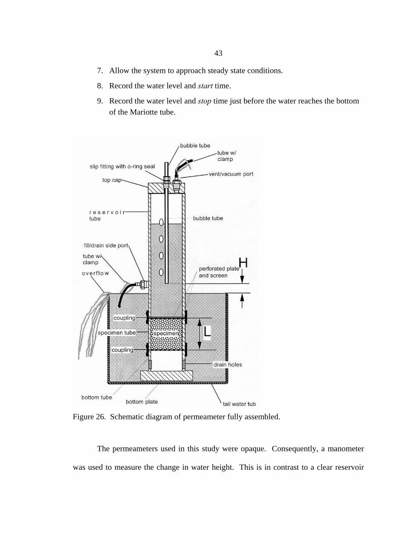
43

7. Allow the system to approach steady state conditions.

8. Record the water level and start time.

9. Record the water level and stop time just before the water reaches the bottom of the Mariotte tube.

Figure 26. Schematic diagram of permeameter fully assembled.

The permeameters used in this study were opaque. Consequently, a manometer

was used to measure the change in water height. This is in contrast to a clear reservoir

44

tube, which could be graduated on the surface. When the reservoir is completely filled,

the water level is above the range measurable by the manometer. The difference in water

level from where the reservoir is completely full to where the water level can be

measured by the manometer is approximately 7 inches, which corresponds to a volume of

approximately 2.3 gallons of water. Each test was started by allowing this initial volume

of water to drain through the sample to allow the system to approach steady state

conditions.

ASTM D2434 and AASHTO T215 suggest that k testing should not be started

until the system completely reaches steady state conditions. However, for the wide range

of particle sizes examined in this study, it was observed that running excessively large

quantities of water through the specimen before testing is started could be counter-

productive. Excessive seepage, especially at high gradients could change the results of

the test because fines could be washed out of the specimen. It was determined that using

a carefully controlled hydraulic gradient and a water volume of 2.3 gallons allowed the

system to approach steady state successfully because only minor changes in k were noted

after this initial volume of water drained through a sample.

Relatively low hydraulic gradients were used on all samples to ensure that the

assumptions inherent in Darcy’s Law were not violated and to provide consistency

between tests. ASTM D2434 recommends applying gradients of 0.2 to 0.3 ft/ft to coarse

grained soils and gradients of 0.3 to 0.5 ft/ft to finer soils. All of the aggregate samples

examined in this study were predominately coarse-grained; consequently, a hydraulic

gradient of 0.26 ft/ft was employed.

45

Results

Saturated permeabilities were determined for each aggregate in this study by

conducting three independent k tests (each using virgin aggregates). Results for each k

test are summarized in Figure 27, and average results for each aggregate type are shown

in Table 11. The COV values shown in Table 11 are relatively large, which is attributed

to the inherently highly variable nature of this parameter. (Values of k are presented in

this section using units of cm/s as is typical practice in the United States. Whenever

practically possible, US Customary units are also presented.)

Figure 27. Summary of permeability (k) test results.

Table 11. Average Permeability (k) Values Based on Aggregate Type Average k Standard Deviation, σ Aggregate

Type (ft/hr) (cm/s) (ft/hr) (cm/s) COV

6A 11.1 0.094 16.9 0.143 1.52 5A 1.5 0.013 1.1 0.009 0.69 2A 10.4 0.088 14.2 0.120 1.36

0.001

0.01

0.1

1

Source Location

Per

mea

bilit

y (c

m/s

)

Billi

ngs

Gle

ndiv

e

Gre

at F

alls

Kal

ispe

ll

Mis

soul

a

But

te

Mis

soul

a

Gre

at F

alls

Kal

ispe

ll

Billi

ngs

Gle

ndiv

e

Lew

isto

wn

Hav

re

Mis

soul

a


1 cm/s = 118.1 ft/hr

This value represents two data points

46

A series of two sample t-tests were performed to facilitate the evaluation of

average k values. The results of this statistical evaluation are presented in Table 12. The

average k values for each aggregate type were all in the same order of magnitude, ranging

from 0.094 to 0.013 cm/s (11.1 to 1.5 ft/hr). The statistical evaluation indicates that 6A

and 2A aggregates both have higher average permeabilities than the 5A aggregates.

There is no statistically significant difference between the average permeabilities of the

2A and 6A samples.

Table 12. Average Permeability (k) Statistical Evaluation Relationship p-value

6A > 5A µ=11.1 µ=1.5

0.986

6A = 2A µ=11.1 µ=10.5

0.552

5A < 2A µ=1.5 µ=10.5 0.015

The measured permeability values fell within typical reported ranges based on

general soil type. Measured values of k for the aggregates in this study varied from 0.002

to 0.529 cm/s (0.23 to 62.5 ft/hr), similar to the approximate ranges reported by Holtz and

Kovacs (1981) for clean sands and gravels.

Estimating Permeability from Grain Size

Background

For course grained materials like those in this study, particle size information is

commonly used for correlation with k. These correlation equations can be unreliable

47

when applied to soils other than those they were developed for (Carrier 2003);

consequently, there is no widely accepted k estimation equation. Several of these grain

size-k correlation equations were evaluated in this study to determine their effectiveness

for use with crushed and processed base course aggregates and for comparison with

laboratory measured permeabilities to further evaluate their reasonableness.

Permeability correlation equations developed for sands and gravels rely on data

obtained from geotechnical index testing to estimate k. Although the parameters used to

determine k vary from equation to equation, they generally rely on particle size and/or

void space measurements of the soil. Table 13 summarizes the six empirical equations

that were evaluated using data measured in this study.

Table 13. Empirical Permeability Correlation Equations Name Year Equation Validity

Hazen 1911 210dCk H= Sands between 0.1 and 3.0

mm

Terzaghi 1925 210

2

3/10

0 )1(13.0 d

nnCk

T⎥⎦

⎤⎢⎣

⎡−−

=µµ

µ Sands with non-uniform

grain size and shape

Moulton 1980 597.0200

654.6478.110

5

)()(10*00219.0

Pndk = Roadway subbase

aggregates

Shahabi et al. 1984 e

edCk u +=

12.1

389.0

10735.0 Medium to fine sand

Chapuis 2004 7825.03

210 1

4622.2 ⎥⎦

⎤⎢⎣

⎡+

=e

edk Saturated sands and gravels

Chapuis 2004 )1(

)1(3max

max32

10

eeeedC

k H

++

= Extended Hazen equation for use on sand or gravel

Notes: CH = empirical coefficient, d10 = grain size corresponding to 10% passing, C/µo = empirical coefficient, µo = dynamic viscosity of water at 10° C, µT dynamic viscosity of the permeant (water) at the temperature of interest, n = porosity, P200 = percent of material passing the No. 200 sieve, Cu = coefficient of uniformity, e = void ratio, and emax = maximum void ratio.

48

Empirical correlation equations for estimating k are best suited for materials that

are similar to those used to develop the equation. The Hazen (1911) equation was

developed for clean filter sands at or near their minimum density (ρmin) with uniformity

coefficients (Cu) of less than 5. The empirical coefficient, CH, in this equation is

generally considered to vary between 0.8 and 1.5. However, Carrier (2003) has shown

that the magnitude of CH can vary over several orders of magnitude when applied to

different granular materials. Hazen’s equation is not expected to perform very well for

the aggregates in this study because they contain effective particle sizes (d10) larger than

the sand that Hazen used to develop his equation, and Cu values greater than 5.

The Terzaghi (1925) equation takes multiple factors into account including

viscosity of the permeant (water) at different temperatures, d10, and n. The empirical

coefficient in this equation, C/µo, varies from 460 for angular sands to 800 for rounded

sands. A value of 460 was used here due to the crushed nature of the aggregates being

examined. This equation was developed for sands with non-uniform grain size and

shape. It is more versatile than Hazen’s equation because it accounts for more factors

that influence k. It is unknown if the Terzaghi equation can be successfully applied to

soils containing particle sizes larger than sand.

The Moulton (1980) equation was developed for roadway subbase aggregates. It

takes multiple factors into account including n and P200. This equation utilizes multiple

factors and was developed for materials similar to those used in this study; consequently,

this equation is expected to perform well.

The Shahabi et al. (1984) and Chapuis (2004) equations are both variants of the

Kozeny-Carman equation, which is given by:

49

⎟⎟⎠

⎞⎜⎜⎝

⎛+

=⎟⎟⎠

⎞⎜⎜⎝

⎛

ee

STkk

p 11 3

20

20γ

µ (4)

where, µ = the dynamic viscosity of the permeant, γp = is the unit weight of the permeant,

ko = the pore shape factor, T = the tortuosity factor, and So = particle shape factor

(Kozeny 1927, Carman 1937).

This equation is widely recognized as a reasonable predictor of k in porous media

such as gravels, sands, and silts (Carrier 2003). The Kozeny-Carman equation is based

on hydraulic principles and takes into account pore shape and size, particle shape and

size, and the tortuosity of the flow path. These parameters are difficult to quantify

because there is no practical way of measuring the tortuosity of the pore space, and most

aggregates contain widely varying pore and particle sizes and shapes, as compared to the

single value the equation accounts for.

Many variations of the Kozeny-Carman equation have been developed that utilize

different methods of experimentally correlating the pore shape/tortuosity/particle shape

term ( 22oo STk ) to more readily measured parameters. The equations presented here from

Shahabi et al. (1984) and Chapuis (2004) are both based on the Kozeny-Carman

equation. Shahabi et al. (1984) assumed that the 22oo STk term depends on d10 and Cu,

while Chapuis (2004) assumed that this term depends solely on d10. The researchers each

used different regression techniques and data sets to develop their equations.

Chapuis (2004) also developed what is known as the “extended Hazen” equation,

which is essentially another variant of the Kozeny-Carman equation. The extended

Hazen equation is nearly the same as the Hazen equation except that it includes a

50

correction factor for the void ratio. Hazen’s equation was developed for loose filter

sands. The term “loose” implies that these sands were at or near emax. The correction

factor was developed by Chapuis (2004) using the e relationship from the Kozeny-

Carman equation to adjust the k of a sample that is at an e other than its emax.

Results

The empirical correlation equations presented in this study utilize grain size data

from mechanical sieve analyses. Two sets of estimated permeabilities are presented; one

set utilizes MSU grain size data, and the other set utilizes MDT grain size data. Figure

28 shows a comparative plot of the predicted and measured k values for the 6A aggregate

type utilizing MSU and MDT grain size data. Differences in k estimations between the

MSU and MDT grain size data are evident in the 6A-Great Falls sample where predicted

values of k are almost an order of magnitude apart from each other. This exemplifies the

dependence of these estimation equations on the finer fraction of the grain size data.

Figure 29 and Figure 30 show comparative plots of the predicted and measured

permeabilities for the 5A and 2A aggregate types, respectively. Permeability estimations

utilizing MDT gradation data could not be created for the 5A-Kalispell sample because

the MDT gradation did not include grain size data with small enough particle sizes to

utilize the estimation equations.

51

Figure 28. Calculated permeabilities for the 6A aggregates.


0.001

0.010

0.100

1.000

Source Location

Per

mea

bilit

y (c

m/s

)

Hazen (1911)Terzaghi (1925)Moulton (1980)Shahabi et al. (1984)Chapuis (2004)Extended Hazen (Chapuis 2004)Measured values

MissoulaBillings Glendive Great Falls KalispellButte

1 cm/s = 118.1 ft/hrValues shown in shaded regions were produced using MDT gradation data.

0.001

0.010

0.100

1.000

Source Location

Per

mea

bilit

y (c

m/s

)


Missoula Great Falls Kalispell


52


Ranges of permeability predicted by the correlation equations varied widely, as

summarized in Table 14. In many cases, the highest and lowest predicted values of k

bracketed the measured k values. This is true of 6A-Butte, 6A-Kalispell, 5A-Great Falls,

5A-Kalispell, 2A-Billings, and 2A-Havre. The k predictions from the Hazen (1911) and

Moulton (1980) equations both tended to fall at or near the upper end of the estimations,

while the k predictions from the Terzaghi (1925) and extended Hazen (Chapuis, 2004)

equations both fell at or near the lower end of the estimations. The equations from

Chapuis (2004) and Moulton (1980) tended to fall somewhere in between these high and

low values.

0.001

0.010

0.100

1.000

Source Location

Per

mea

bilit

y (c

m/s

)


LewistownBillings Glendive MissoulaHavre


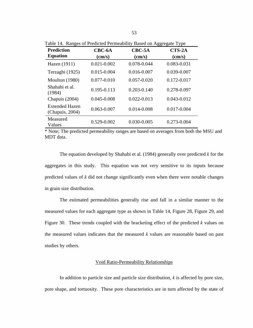
53

Table 14. Ranges of Predicted Permeability Based on Aggregate Type CBC-6A CBC-5A CTS-2A Prediction

Equation (cm/s) (cm/s) (cm/s) Hazen (1911) 0.021-0.002 0.078-0.044 0.083-0.031 Terzaghi (1925) 0.015-0.004 0.016-0.007 0.039-0.007 Moulton (1980) 0.077-0.010 0.057-0.020 0.172-0.017 Shahabi et al. (1984) 0.195-0.113 0.203-0.140 0.278-0.097

Chapuis (2004) 0.045-0.008 0.022-0.013 0.043-0.012 Extended Hazen (Chapuis, 2004) 0.063-0.007 0.014-0.008 0.017-0.004

Measured Values 0.529-0.002 0.030-0.005 0.273-0.004

* Note; The predicted permeability ranges are based on averages from both the MSU and MDT data.

The equation developed by Shahabi et al. (1984) generally over predicted k for the

aggregates in this study. This equation was not very sensitive to its inputs because

predicted values of k did not change significantly even when there were notable changes

in grain size distribution.

The estimated permeabilities generally rise and fall in a similar manner to the

measured values for each aggregate type as shown in Table 14, Figure 28, Figure 29, and

Figure 30. These trends coupled with the bracketing effect of the predicted k values on

the measured values indicates that the measured k values are reasonable based on past

studies by others.

Void Ratio-Permeability Relationships

In addition to particle size and particle size distribution, k is affected by pore size,

pore shape, and tortuosity. These pore characteristics are in turn affected by the state of

54

compaction. For cohesionless soils, the state of compaction is often quantified on a

macro basis by void ratio (e). The permeameter samples in this study were each

compacted using the same compaction energy and methodology; however, because of

differences in particle size, shape, and distribution, the compacted void ratios varied

slightly between samples. Because of the dependency of k on void structure, a

relationship between e and k was explored. When all soil samples are examined together,

there is not a very strong correlation between e and k, as shown in Figure 31. This

indicates that k cannot be predicted solely on the basis of compacted density or e.

Figure 31. Void ratio versus permeability for all aggregates in this study.

The value of e commonly used to calculate k is the average e determined from

weight-volume relationships using total weight and total volume data. Cote and Konrad

(2003) proposed that because k is known to highly depend on smaller particles, it could

y = 0.0068Ln(x) + 0.3871R2 = 0.0442

0.25

0.30

0.35

0.40

0.45

0.50

0.55

0.001 0.010 0.100 1.000Permeability (cm/s)

Voi

d R

atio

(e)

kef

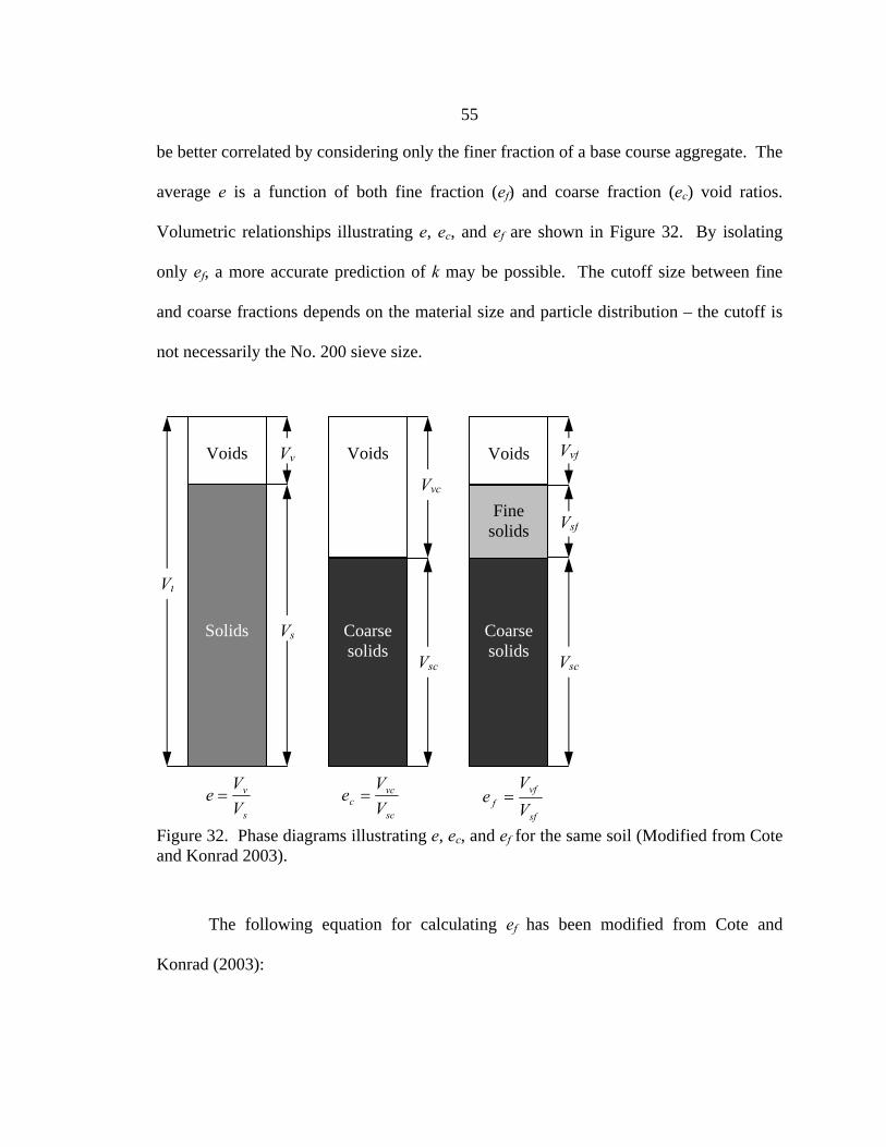
55

be better correlated by considering only the finer fraction of a base course aggregate. The

average e is a function of both fine fraction (ef) and coarse fraction (ec) void ratios.

Volumetric relationships illustrating e, ec, and ef are shown in Figure 32. By isolating

only ef, a more accurate prediction of k may be possible. The cutoff size between fine

and coarse fractions depends on the material size and particle distribution – the cutoff is

not necessarily the No. 200 sieve size.

Figure 32. Phase diagrams illustrating e, ec, and ef for the same soil (Modified from Cote and Konrad 2003).

The following equation for calculating ef has been modified from Cote and

Konrad (2003):

Voids

Solids

Voids

Coarsesolids

Coarsesolids

Fine solids

Voids

Vt

Vs

Vv

Vsc

Vvc

Vvf

Vsf

Vsc

s

v

VV

e =sc

vcc V

Ve =

sf

vff V

Ve =

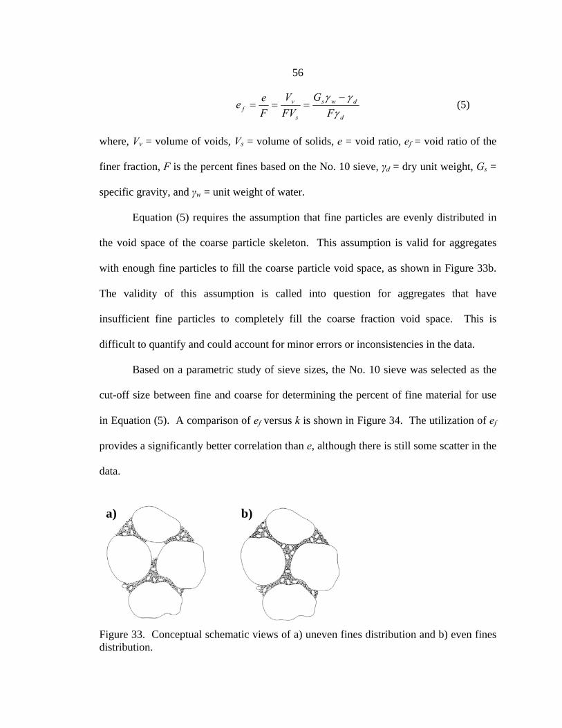
56

d

dws

s

vf F

GFVV

Fee

γγγ −

=== (5)

where, Vv = volume of voids, Vs = volume of solids, e = void ratio, ef = void ratio of the

finer fraction, F is the percent fines based on the No. 10 sieve, γd = dry unit weight, Gs =

specific gravity, and γw = unit weight of water.

Equation (5) requires the assumption that fine particles are evenly distributed in

the void space of the coarse particle skeleton. This assumption is valid for aggregates

with enough fine particles to fill the coarse particle void space, as shown in Figure 33b.

The validity of this assumption is called into question for aggregates that have

insufficient fine particles to completely fill the coarse fraction void space. This is

difficult to quantify and could account for minor errors or inconsistencies in the data.

Based on a parametric study of sieve sizes, the No. 10 sieve was selected as the

cut-off size between fine and coarse for determining the percent of fine material for use

in Equation (5). A comparison of ef versus k is shown in Figure 34. The utilization of ef

provides a significantly better correlation than e, although there is still some scatter in the

data.

Figure 33. Conceptual schematic views of a) uneven fines distribution and b) even fines distribution.

a) b) a) b)

57

Figure 34. Fine fraction void ratio (ef) versus permeability.

Several other correlations were examined using Cu, Cc, and d10; however, none of

these other parameters were effective at reducing R2. This suggests that hydraulic

properties of an aggregate rely more heavily on pore parameters than particle parameters.

According to Equation (5), ef is a function of e and F, which is derived from the grain

size distribution (percent fines based on the No. 10 sieve). Aggregate compaction is

often specified as some percentage of a maximum laboratory determined density or unit

weight. Combining the logarithmic regression shown in Figure 34 with Equation (5)

yields an equation that can be used for estimating k for base course materials used by

MDT from readily assumed or measured parameters, and is shown as:

77.10117.01ln

max

−⎥⎦

⎤⎢⎣

⎡−=

d

ws

RCG

Fk

γγ (6)

y = 0.1732Ln(x) + 1.8629R2 = 0.6213

0.40

0.60

0.80

1.00

1.20

1.40

1.60

1.80

2.00

2.20

2.40

0.001 0.010 0.100 1.000

Permeability (cm/s)

Fine

Fra

ctio

n Vo

id R

atio

(ef)

ef k

58

where, k is the permeability in cm/s, F is the percent material finer than the No. 10 sieve,

Gs is the specific gravity, γw is the unit weight of water in pcf, γd max is the maximum unit

weight in pcf, and RC is the relative compaction.

This equation could be useful for comparing the hydraulic properties of base

course aggregates, for estimating the hydraulic properties of materials that are out of

specification, or to determine the maximum amount of material passing the No. 10 sieve

to achieve a particular minimum k.

Equation (6) can be re-arranged to compute F (the maximum amount of material

passing the No. 10 sieve) if Gs, γd max, the required RC, and the required minimum k are

all known. This is a useful application of the equation for developing material

specifications, and is presented as:

⎥⎦

⎤⎢⎣

⎡−⎥⎦

⎤⎢⎣⎡

+= 1

83.1ln17.01

maxd

ws

RCG

kF

γγ (7)

The following steps outline the calculation procedure:

1. Determine γd max from either maximum index density or modified Proctor testing.

2. Assume a value for RC. MDT commonly uses 0.95 to 0.98.

3. Measure Gs in the lab, or assume a value of about 2.7.

4. Select a minimum value of k. This value should be selected so that it is practically achievable, and will provide adequate drainage capacity.

5. Table 15 shows AASHTO (1993) design guide recommended minimum permeabilities.

6. Substitute the above parameters into Equation (7) to determine the maximum amount of material passing the No. 10 sieve.

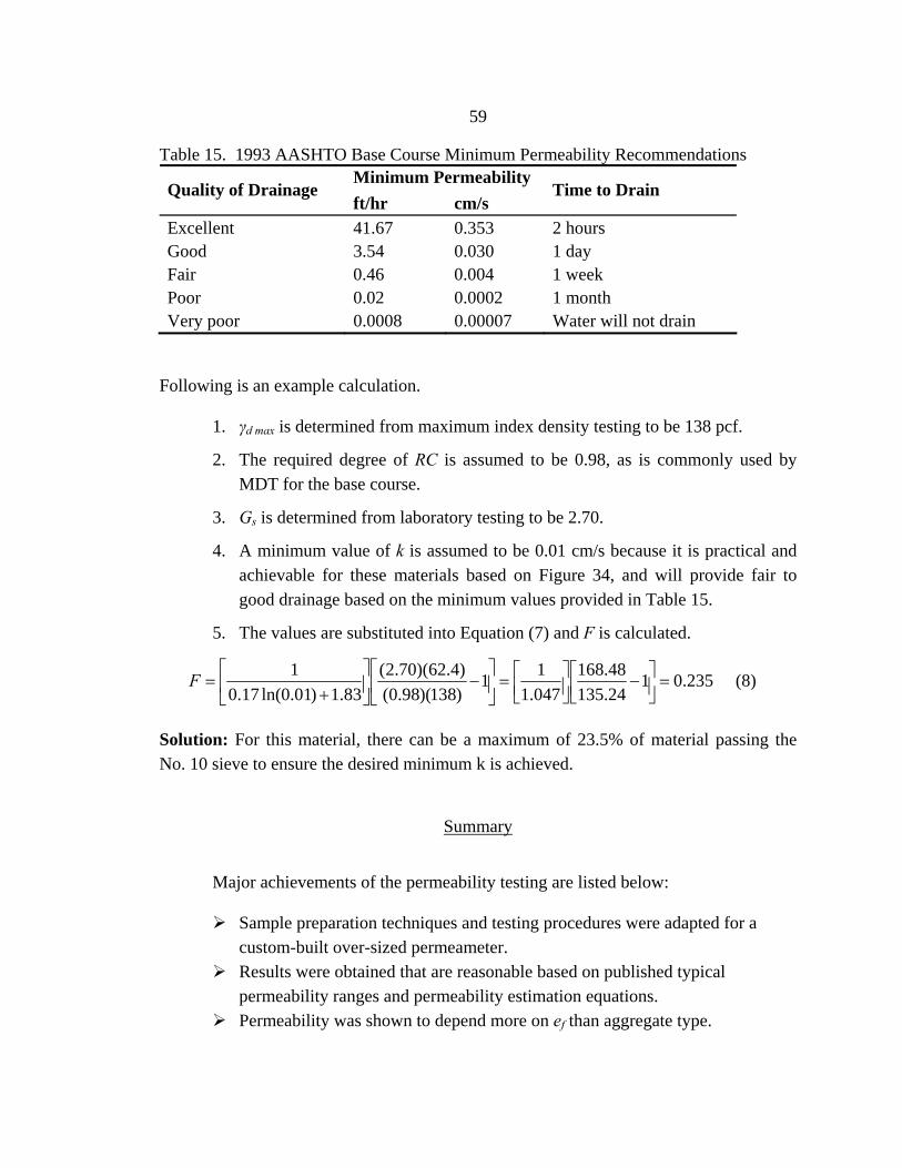
59

Table 15. 1993 AASHTO Base Course Minimum Permeability Recommendations Minimum Permeability

Quality of Drainage ft/hr cm/s

Time to Drain

Excellent 41.67 0.353 2 hours Good 3.54 0.030 1 day Fair 0.46 0.004 1 week Poor 0.02 0.0002 1 month Very poor 0.0008 0.00007 Water will not drain

Following is an example calculation.

1. γd max is determined from maximum index density testing to be 138 pcf.

2. The required degree of RC is assumed to be 0.98, as is commonly used by MDT for the base course.

3. Gs is determined from laboratory testing to be 2.70.

4. A minimum value of k is assumed to be 0.01 cm/s because it is practical and achievable for these materials based on Figure 34, and will provide fair to good drainage based on the minimum values provided in Table 15.

5. The values are substituted into Equation (7) and F is calculated.

235.0124.13548.168

047.111

)138)(98.0()4.62)(70.2(

83.1)01.0ln(17.01

=⎥⎦⎤

⎢⎣⎡ −⎥⎦

⎤⎢⎣⎡=⎥

⎦

⎤⎢⎣

⎡−⎥

⎦

⎤⎢⎣

⎡+

=F (8)

Solution: For this material, there can be a maximum of 23.5% of material passing the No. 10 sieve to ensure the desired minimum k is achieved.

Summary

Major achievements of the permeability testing are listed below:

Sample preparation techniques and testing procedures were adapted for a custom-built over-sized permeameter.

Results were obtained that are reasonable based on published typical permeability ranges and permeability estimation equations.

Permeability was shown to depend more on ef than aggregate type.

60

X-RAY COMPUTED TOMOGRAPHY

The primary goal of X-ray computed tomography (CT) scanning in this study was

to non-destructively acquire and subsequently measure 2-dimensional (2D) slice images

of aggregate samples to estimate/measure their properties. The soil properties of interest

were the void ratio (e), grain size distribution, and pore size distribution. Grain size

distributions were previously measured using traditional geotechnical techniques, and e

can be calculated from weight-volume relationships. These same properties were

estimated from X-ray CT data in order to test/confirm the applicability of the MSU X-ray

CT scanning system for these purposes. The pore size distribution was measured to

discern differences between aggregate types and to further the understanding of the

internal structure/behavior of crushed and processed aggregates. In addition, image

thresholding methods were developed to further refine soils image processing techniques.

The MSU X-ray CT scanner and scanning software exclusively use SI units. For

this reason, SI units will be the primary units presented in the following X-ray CT

sections.

History & Applications

X-ray CT was first developed in the late-1970’s for use in the medical field to

obtain 2D and 3D images of internal body organs and tissues. X-ray beam power was

limited to approximately 125 kV with relatively short exposure times to minimize tissue

damage. X-ray CT technology was adapted for industrial uses in the 1980’s. Uninhibited

by exposure time and power limitations inherent in medical scanning, X-ray beam

61

powers in excess of 400 kV were possible. This allowed for significantly better

resolutions than those attainable by medical scanners, and facilitated a wide variety of

applications for X-ray CT. These applications included the internal imaging of

irreplaceable paleontology specimens (Conroy and Vannier 1984) and one-of-a-kind

meteorites (Arnold et al. 1982). In the mid-1980’s and early-1990’s, X-ray CT

applications in the geo-sciences were also developed. As X-ray CT scanners evolved and

improved over the years, so have the vastness of applications of this technology.

Ketcham and Carlson (2001) noted that the applications of X-ray CT to the geo-sciences

were still only in their infancy as of the time of publishing.

X-ray CT has been used in the geotechnical and geologic fields to study a wide

variety of topics. Steude et al. (1994) provides a comprehensive list of the early uses of

industrial X-ray CT. Several more recent examples are provided by Ketcham and

Carlson (2001) and Alramahi and Alshibli (2006). Several of the most recently studied

geotechnical topics include the formation and propagation of shear bands in sand during

triaxial testing (Alshibli et al. 2000, Desrues et al. 1996), and various flow and moisture

properties of soil and rock (Fukahori 2003, Cislerova 2002). Researchers have attempted

to use computer software to model flow properties of soil and asphalt cores using 3D X-

ray CT particle and compaction information (Kutay et al. 2006). Unfortunately, this

software is highly complex and is still in developmental stages.

Alternative methods for acquiring 2D slice images of soil or rock cores, such as

serial sectioning, are destructive (Ketcham and Carlson 2001). The serial sectioning

process involves impregnating a soil sample with low viscosity epoxy and physically

cutting the object into thin slices and measuring those slices. This process is expensive,

62

time consuming, and can alter the internal features of a soil sample. X-ray CT can also

be expensive initially due to the high capital cost of equipment. Additionally, X-ray CT

is considerably faster than serial sectioning once equipment is set-up and calibrated, and

X-ray CT provides digitized results that can be easily measured and stored, which makes

it suitable for quantitative analyses.

The non-destructive nature of X-ray CT represents a significant advantage over

traditional methods of acquiring 2D internal slice images of soil and rock cores. Non-

destructive testing allows multiple tests to be run on one sample without changing the

structure of that sample. Similarly, the same sample can be tested while undergoing

small incremental changes, like changes in water content or stress state, to quantify the

effect of these changes.

Acquiring Images: How it Works

X-ray CT scanning consists of basically two phases: image acquisition and image

reconstruction. The MSU X-ray CT scanner is a 3rd generation scanner based on a

classification system proposed by Ketcham and Carlson (2001). The MSU Scanner is

capable of both centered and off-set geometries, though centered geometry is almost

exclusively used. A schematic diagram of the major system components is shown in

Figure 35. The scanning system consists of: i) an X-ray source that produces a fanned

beam of X-rays, ii) lead collimator plates that shape the rough X-ray fan beam to a more

precise thin fan of X-rays, iii) the object being scanned that rests on a rotating table, iv)

another set of lead collimator plates to shape the X-ray fan beam, v) a phosphor screen,

which converts X-ray beams into visible light, and vi) a digital camera for capturing

63

images of the illuminated phosphor screen during scanning. The variation in the amount

of light given off at different locations along the phosphor screen is directly proportional

to the extent that the X-ray beam has been attenuated by the object.

Figure 35. Schematic plan view of MSU 3rd generation CT scanner.

One camera image for a particular orientation of the object is termed a “view”,

which appears as a thin strip of pixels of varying brightness. A simplified “view” of

several concentric circles of varying density is shown in Figure 36a. Many views must

be acquired at different degrees of rotation to produce one final 2D slice image of an

object. The smaller the degree of rotation between views, the higher resolution the final

2D slice image will be.

64

Figure 36. Image reconstruction: a) single view, b) projection of single view, c) over-layed and rotated projected views, and d) same as c with more projected views (from Nielson and Mokwa 2004).

After images are acquired, they must be reconstructed. The first step in image

reconstruction is projection. In this step, each view is projected to the full diameter of the

spacimen, as shown in Figure 36b. Projected views are then rotated to the angle in which

they were acquired and overlain on top of one another, as shown in Figure 36c and Figure

36d. Figure 37 shows different reconstructions of the same object each using different

numbers of views. It can be seen in these 2D slice images that the clarity of the object is

dramatically increased by increasing the number of views used to reconstruct the 2D slice

image. Increasing the number of views is analogous to decreasing the degree of rotation

between subsequent views.

a) b) c) d)

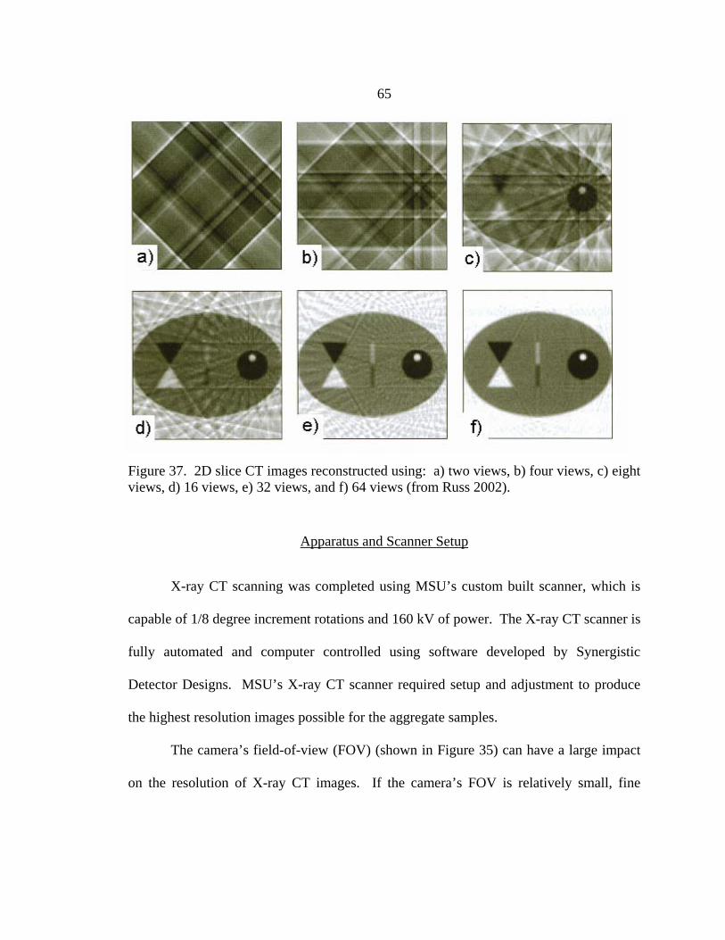
65

Figure 37. 2D slice CT images reconstructed using: a) two views, b) four views, c) eight views, d) 16 views, e) 32 views, and f) 64 views (from Russ 2002).

Apparatus and Scanner Setup

X-ray CT scanning was completed using MSU’s custom built scanner, which is

capable of 1/8 degree increment rotations and 160 kV of power. The X-ray CT scanner is

fully automated and computer controlled using software developed by Synergistic

Detector Designs. MSU’s X-ray CT scanner required setup and adjustment to produce

the highest resolution images possible for the aggregate samples.

The camera’s field-of-view (FOV) (shown in Figure 35) can have a large impact

on the resolution of X-ray CT images. If the camera’s FOV is relatively small, fine

66

details will be captured in the resulting images, and if the camera’s FOV is relatively

large, detail is lost but larger objects can be scanned.

Particles of the 6A and 5A soil samples larger than 19.1 mm (0.75 inches) were

screened and removed to reduce the sample container size, thereby reducing the camera’s

FOV and improving the resolution. Modification of the 2A samples was not necessary.

The same container size was utilized for all samples so that all images had the same

resolution, and maintained the same container diameter to maximum particle size (d:p)

ratio. A container diameter of 76.2 mm (3 inches) was selected, which provided a d:p

ratio of 4:1, and a resolution of approximately one pixel = 0.080 mm.

Nine scans were completed on each cylindrical sample at a spacing of one scan

every 9.00 mm. Scans were not taken within 38 mm of the top or bottom of the container

to avoid heterogeneities near these boundaries. Multiple scans were taken of each sample

so that properties measured from each scan location could be averaged together to

account for variations across the sample due to unavoidable minor segregation. The

number of scans was limited to nine to keep scanning time within reason, while still

providing accurate results. Each scan took approximately two hours, for a total of more

than 20 hours required to fully scan each sample.

The highest power setting (160 kV) on the MSU X-ray CT scanner was used with

camera exposure times of approximately 3.6 seconds. High power was necessary to fully

penetrate samples because of the high density of the soil and rock samples being scanned

and the relatively large size of the sample containers. Camera exposure times were set as

long as possible to achieve the highest resolution possible, while preventing the

saturation of pixels in the resulting digital images.

67

The increment of sample rotation between the acquisition of each view effects the

resolution. The MSU X-ray CT scanner is capable of producing 1/8 degree increment

scans. However, 1/4 degree scans were utilized in this study because the increase in

resolution realized in 1/8 degree scanning was negligible, and 1/4 degree scans required

significantly less acquisition and processing time. Scanning at 1/4 degree increments

produced 1,440 views requiring reconstruction to produce one final 2D slice image of the

soil sample.

These settings provided the highest resolution achievable by the MSU X-ray CT

scanner with the samples being tested. Nielson and Mokwa (2004) provide additional

details regarding soil sample imaging using the MSU X-ray CT scanner.

Sample Preparation

Meticulous care was taken during the preparation, placement, and compaction of

samples to minimize segregation. All samples were compacted in four evenly sized lifts

of approximately 400 grams each. Each lift received 20 drops from a 24.4-N rammer

from a height of 152.4 mm, which equates to 409.9 kN-m/m3 of compaction energy.

Samples were prepared dry so that only two phases (solid and gas) were present in the

samples for X-ray CT scanning, as compared to the three phases that would have to be

discerned in X-ray CT images if samples were compacted moist.

Image Processing

All image processing was completed using ImageJ image analysis software,

which was developed by the National Institutes of Health and is available at no charge

68

from http://rsb.info.nih.gov/ij. Image processing of 2D X-ray CT images involves the

following basic steps: despeckling, thresholding, and measuring/analysis.

Despeckling

After image acquisition and re-construction, all 2D slice images were despeckled.

This process smoothes the images by removing some of the noise present. This is

accomplished in the software by measuring pixel intensities in a 3x3 grid around a given

pixel and assigning this center pixel the median value of the surrounding pixels (Russ

2002). This process is completed for each pixel in the digital image. The despeckling

command can be found in ImageJ in the following menus: Process – Noise – Despeckle.

Despeckled images of the aggregate samples are provided in Appendix D.

Thresholding

The next image processing step is referred to as thresholding. Each pixel in an 8-

bit X-ray CT image represents some grayscale value from 0 to 255, where 0 represents

white or void space and 255 represents black or solid space. In order to take meaningful

measurements, each pixel must be deemed either void or solid space. A cut-off threshold

grayscale value must be determined to assign all pixels the distinction of either void or

solid. Figure 38 shows two images, one before thresholding and one after. The

corresponding histogram of pixel intensities is shown in Figure 38c. This histogram has

the threshold value used to produce the image in Figure 38b indicated on the x-axis. The

original image has a wide variety of pixel intensities, while the thresholded image has

only white (0, void) or black (255, solid) pixels. The thresholding command can be

found in ImageJ in the following menus: Image – Adjust – Threshold.

69

Figure 38. Thresholding example: a) original image, b) thresholded image, and c) pixel intensity histogram with threshold value indicated on the x-axis.

There are no well established guidelines for determining the threshold value for

soil X-ray CT images. Images are commonly thresholded in a subjective manner by

visually adjusting the threshold value until void and solid space appear to match the

original image, which leads to variance between the thresholding of different images and

between different operators. In scanning soil samples with particles of varying density

and size, a threshold value that visually makes all known solid objects completely black

may also misclassify some of the solid space as void, as shown in Figure 39. The image

in Figure 39b still exhibits some void pixels in areas that are actually solid space, as

indicated by the circles, despite the fact that very few void pixels can be seen in the rest

a) b)

c)

70

of the image. This phenomenon occurs because the measured void and solid pixel

intensities partially overlap, which can at least partially be attributed to partial volume

effects.

Figure 39. Thresholding example where void pixels in identified solid areas are minimized: a) original image, b) thresholded image, and c) pixel intensity histogram with threshold value indicated on the x-axis.

Each pixel in a 2D X-ray CT image represents a specific quantification of area. In

this study, one pixel = 0.080 mm. If this area is occupied by several different materials,

the resulting measured pixel intensity will represent some average of these different

materials. In other words, if an image is acquired with several small particles (with some

b)a)

c)

71

air space in between them) in one pixel, then the pixel intensity produced will not

represent solid or void, but rather some average of the two.

One of the subordinate goals of this research was to develop a more objective

means of thresholding soil X-ray CT images. It is hypothesized that choosing a threshold

value based on the histogram of grayscale pixel intensities will produce a more accurate

and consistent final thresholded image. Pixel intensity histograms typically have a nearly

normal distribution, with occasional slightly positive or negative skews (Figure 39c).

The following statistical terms will be used in subsequent discussions:

Average, ∑=

=N

iix

N 1

1µ

Mode, M, the most frequently occurring value in a histogram

Standard deviation, ∑=

−=N

iix

N 1

2)(1 µσ

Pearson’s 1st skewness coefficient, σ

µ Ms −= 3

Several options were weighed in developing a formula for determining threshold

values. The following two formulas were carefully considered after a parametric study

was conducted to determine the primary factors for consideration:

σµ 6.0−=T (9)

σ6.0−= MT (10)

where, T = threshold value. The value of 0.6 was determined by trial and error and

provided reasonable results for the soil images in this study. Initially, Equation (9) and

Equation (10) were both used to determine threshold values for five of the soil samples

(2A-Billings, 6A-Billings, 5A-Great Falls, 6A-Kalispell, and 6A-Missoula). Values of e

72

produced using these two thresholding equations were compared to the weight-volume

determined e values. Equation (10) generally produced more accurate results, as shown

in Figure 40. Equation (9) did not seem to be very sensitive to inputs because it produced

values of e that were between 0.3 and 0.4 for all images/samples.

An in-depth sensitivity analysis was outside the scope of this study, but the

following recommendation is provided for future work in this area. The values of e

produced by Equation (10) appears to be inversely related to s. Therefore, it is

hypothesized that incorporating some factor of s into Equation (10), possibly in place of

the constant value of 0.6, may produce better results.

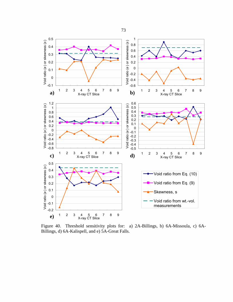
73

Figure 40. Threshold sensitivity plots for: a) 2A-Billings, b) 6A-Missoula, c) 6A-Billings, d) 6A-Kalispell, and e) 5A-Great Falls.

-0.6

-0.4

-0.2

0

0.2

0.4

0.6

0.8

1

1 2 3 4 5 6 7 8 9X-ray CT Slice

Voi

d ra

tio (e

) or s

kew

ness

(s)

b)

-0.8-0.6-0.4-0.2

00.20.40.60.8

11.2

1 2 3 4 5 6 7 8 9X-ray CT Slice

Voi

d ra

tio (e

) or s

kew

ness

(s)

c) -0.5-0.4-0.3-0.2-0.1

00.10.20.30.40.50.6

1 2 3 4 5 6 7 8 9X-ray CT Slice

Voi

d ra

tio (e

) or s

kew

ness

(s)

d)

-0.2

-0.1

0

0.1

0.2

0.3

0.4

0.5

1 2 3 4 5 6 7 8 9X-ray CT Slice

Void

ratio

(e) o

r ske

wne

ss (s

)

e)

-0.1

0

0.1

0.2

0.3

0.4

0.5

1 2 3 4 5 6 7 8 9X-ray CT Slice

Voi

d ra

tio (e

) or s

kew

ness

(s)

a)

e from Eq. (10)

e from Eq. 9

skewness, s

e from wt.-vol.measurements

Void ratio from Eq. (10)

Void ratio from Eq. (9)

Skewness, s

Void ratio from wt.-vol.measurements

74

Void Ratio Analysis

Void ratio (e) was calculated from the 2D thresholded images by counting the

number of void and the number of solid pixels in each image. From these pixel counts,

values of e can be calculated using the following equation:

pixelssolidofNumberpixelsvoidofNumbere = (11)

Calculated e values for each of the nine images were averaged together for each

aggregate sample. Values of e determined from the X-ray CT images are compared to e

values determined from weight-volume relationships in Figure 41. Values of e estimated

from X-ray CT images generally exhibited relatively small variances between the nine

images measured for each sample. There are three exceptions (6A-Billings, 6A-

Missoula, and 2A-Lewistown) that exhibited relatively large variations in CT estimated e

values between different slices of the same sample. In two other samples (5A-Missoula

and 2A Missoula), the weight-volume measured e did not fall in the range of the X-ray

CT estimated values.

High variance or inaccuracies in the X-ray CT measured e values are attributed to

the segregation of particles during placement and compaction, as well as thresholding

techniques. Known inaccuracies in the measured images include partial volume effects

and ring artifacts. Ring artifacts (Figure 38 and Figure 39) proved difficult to remove

from the images, and are likely the result of a number of factors related to changes in the

way the phosphor converting screen responds to changes in beam strength during a single

CT scan. These changes in beam strength could be due to environmental conditions, such

75

as temperature or humidity, or variations in beam hardness as the sample rotates

(Ketcham and Carlson 2001). Beam hardness causes the edges of an object to appear

brighter than the center because lower energy X-rays are attenuated more easily than

higher energy ones. Consequently, the average energy of the beam is changed after

passing through an object.

Figure 41. X-ray CT and weight-volume void ratio comparison.

Grain Size Analysis

Grain size distributions were calculated from the thresholded 2D X-ray CT

images using granulometry and stereology. Granulometry and stereology are image

processing and statistical methods used to determine grain or pore size distributions from

2D soil images.

0

0.2

0.4

0.6

0.8

1

1.2

Source Location

Voi

d R

atio

(e)

Weight-Volume

CT Average

CT Maximum and Minimum

Bill

ings

Gle

ndiv

e

Gre

at F

alls

Kal

ispe

ll

Mis

soul

a

But

te

Mis

soul

a

Gre

at F

alls

Kal

ispe

ll

Bill

ings

Gle

ndiv

e

Lew

isto

wn

Hav

re

Mis

soul

aCBC-6A CBC-5A CTS-2A

76

The granulometry procedure involves many steps of “opening” an image and then

measuring it. In 2D image processing, the process of opening an image results in the

smallest particles being eliminated from the image. Before and after each opening, the

number of solid pixels is counted. The difference in solid pixels before and after the

opening indicates the number of particles that were contained in the size that was

eliminated from the image. Openings are performed that remove increasingly large

particle sizes, until all particles have been removed from the image.

The data collected in the granulometry procedure is collected from 2D images;

however, grain size distributions are representative of 3D objects. Stereology is defined

as the science of estimating 3D properties from 2D images. A series of statistical

procedures are used to adjust granulometry data such that it approximately represents 3D

objects. Mokwa and Nielson (2004) present additional details regarding granulometry

and stereology procedures.

Before the granulometry and stereology analysis was performed, additional image

processing was conducted to improve the accuracy of the results. During thresholding, it

was visually apparent that some solid space was misclassified as void space (Figure 38b).

To improve the accuracy of the process, images were closed one time to eliminate the

smallest pore sizes. This resulted in the elimination of much of the misclassified void

space. Remaining visually apparent misclassified void space was removed by hand.

Example images from before and after this closing are shown in Figure 42. This

additional step produced more accurate grain size distributions for larger particle sizes,

but also reduced the resolution and consequently produced less accurate grain size

distributions for smaller particle sizes.

77

Figure 42. Image processing steps before grain size analysis: a) despeckled image, b) thresholded image, c) image after closing and removal of misclassified void pixels.

Grain size distributions were relatively accurate from the maximum particle size

down to approximately 1 or 2 mm, although particles in this size range were represented

slightly smaller than indicated by mechanical sieve analysis. This is likely due to some

remaining pixels that are misclassified as void. These out-of-place pixels added noise to

the images, and if located within a larger particle, caused that particle to be counted as a

series of smaller particles. For particle sizes smaller than 1 to 2 mm, the X-ray CT grain

b)

c)

a)

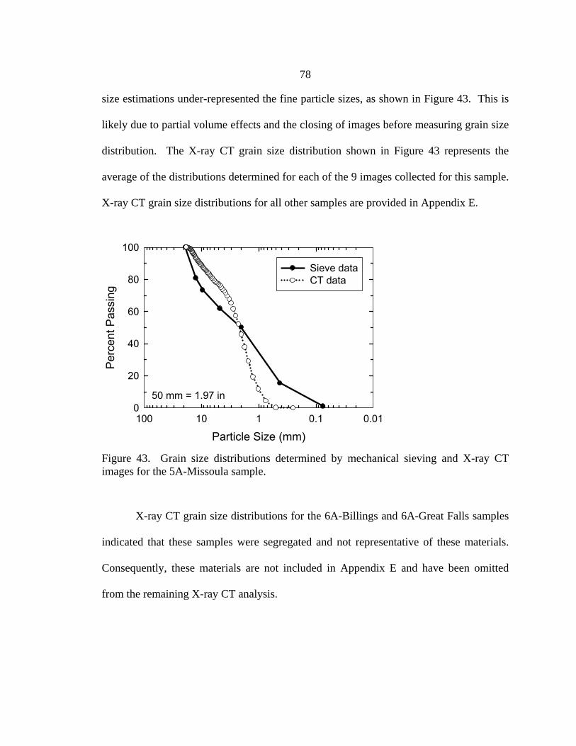
78

size estimations under-represented the fine particle sizes, as shown in Figure 43. This is

likely due to partial volume effects and the closing of images before measuring grain size

distribution. The X-ray CT grain size distribution shown in Figure 43 represents the

average of the distributions determined for each of the 9 images collected for this sample.

X-ray CT grain size distributions for all other samples are provided in Appendix E.

Figure 43. Grain size distributions determined by mechanical sieving and X-ray CT images for the 5A-Missoula sample.

X-ray CT grain size distributions for the 6A-Billings and 6A-Great Falls samples

indicated that these samples were segregated and not representative of these materials.

Consequently, these materials are not included in Appendix E and have been omitted

from the remaining X-ray CT analysis.

50 mm = 1.97 in

Particle Size (mm)0.010.1110100

Perc

ent P

assi

ng

0

20

40

60

80

100

Sieve dataCT data

50 mm = 1.97 in

79

Pore Size Analysis

Pore size distributions were calculated from the same thresholded and closed X-

ray CT images by inverting the black and white pixels so that pore space was highlighted

instead of grain space. The same granulometry and stereology procedures were used.

Pore size distributions for 6A, 5A, and 2A samples are shown in Figure 44, Figure 45,

and Figure 46, respectively.

Figure 44. CBC-6A pore size distributions.

Pore Size (mm)

0.1110

Perc

ent P

assi

ng

0

20

40

60

80

100

Butte GlendiveKalispell Missoula

50 mm = 1.97 in

80

Figure 45. CBC-5A pore size distributions.

Figure 46. CTS-2A pore size distributions.

No secondary pore size distribution data was available to compare the X-ray CT

data with. An abrupt change of slope in many of the pore-size curves occurs at

Pore size (mm)0.1110

Perc

ent P

assi

ng

0

20

40

60

80

100

Missoula Glendive Havre Lewistown Billings

50 mm = 1.97 in

Pore Size (mm)

0.1110

Perc

ent P

assi

ng

0

20

40

60

80

100

Great Falls KalispellMissoula

50 mm = 1.97 in

81

approximately 0.2 to 0.4 mm. This change of slope is thought to occur largely due to

partial volume effects and appears to represent the limit of accuracy for the pore size

distributions. This abrupt change of slope can clearly be seen in the following samples:

6A-Glendive, 6A-Butte, 6A-Kalispell, 2A-Havre, and 2A-Glendive. All other samples

exhibited pore sizes that were mostly larger than this value and there is consequently no

abrupt change of slope visible.

Pore size distributions do not seem to be closely correlated to material type;

consequently, no differences based on aggregate type could be discerned.

Estimating Permeability from Pore Size Distribution

Background

Studies by Vervoot (2003) and Cote and Konrad (2003) indicate that pore

parameters may exert more influence than grain size parameters on the hydraulic

properties of soils. Several attempts have been made at correlating pore size distributions

to permeability (Marshall 1958, Garcia-Bengochea 1979). Many of these correlations

have been developed for fine-grained soils (particle sizes from clays to sands), but none

for open-graded base course aggregates containing few fines. This is attributed to past

difficulties in determining pore size distributions for open-graded aggregates containing

few fines.

Pore size distributions can be determined for open-graded base course aggregates

using relatively recently developed techniques that utilize X-ray CT. Other methods for

determining pore size distributions of soils include correlation with the soil water

characteristic curve (SWCC) and mercury intrusion. The SWCC method involves

82

measurement of the relationship between water content and matric suction, and relies on

the assumption that matric suction is related to pore radii. This method for determining

pore size parameters is not practical for large pore sizes such as those found in base

course aggregates because large pores can drain under gravity alone. Mercury intrusion

involves introducing mercury into a dry soil specimen and measuring the mercury content

of the soil sample under different mercury pressures. This method is no longer used due

to the toxicity of mercury.

Results

The pore size of 80% passing (p80) was used for correlation with k because this

parameter occurred closer to the upper portion of the pore size distributions where data is

thought to be more reliable, yet low enough on the curves to be a value that is

representative of the entire material sample. The pore size of 80% passing correlates well

with k, as shown in Figure 47. Permeability values presented in Figure 47 are averages of

the three k tests performed on each sample. Data from the 6A-Billings and 6A-Great

Falls samples were not included in this correlation because they represented dramatic

outliers. These outliers likely occur because particle sizes larger than 19.1 mm (0.75

inches) were screened off of the 6A samples for CT scanning, thereby significantly

altering the properties of these aggregate samples.

83

Figure 47. Pore size of 80% passing (p80) versus permeability (k) plot.

Several other pore size parameter correlations were examined including the pore

size of 90% passing and the percent passing the No. 10 and No. 40 sieve sizes. These

pore size parameters were near the upper end of the pore size distributions, where data for

all of the samples was considered most reliable. Some distributions did not produce

reliable data for sizes any smaller than approximately the No. 40 sieve size. It is

hypothesized that this correlation could be improved if smaller pore information could be

included. Based on the data evaluation shown in Figure 47, the following equation is

presented for estimating k for base course materials used by MDT:

29.0

89.1ln 80 −=

pk (12)

y = 0.2916Ln(x) + 1.8859R2 = 0.8349

0.0

0.2

0.4

0.6

0.8

1.0

1.2

1.4

1.6

1.8

2.0

0.001 0.010 0.100 1.000

Permeability (cm/s)

Por

e si

ze o

f 80%

pas

sing

, p80

(mm

)

kef

84

where p80 is in mm and k is in cm/s. This equation could be useful for making

approximate comparisons of k between different MDT crushed aggregates, or for

estimating k for out-of-specification materials.

The p80 correlation presented in Figure 49 has an even better R2 value (0.84) than

the ef correlation presented in Figure 39, which had and R2 value of 0.62. This indicates

that using the p80, which is derived from the pore size distribution, is more strongly

correlated to hydraulic properties than ef. While ef is related to pore information, it is

derived from weight-volume and grain size information. The correlations presented here

relating k to pore parameters also provide significantly better correlations than the

published equations that were evaluated in Figure 32, Figure 33, and Figure 34, which

rely largely on grain size information. This shows that the hydraulic properties of

crushed base course aggregates (with few fines) depend more on pore parameters than

grain parameters.

Summary

Major achievements of the X-ray CT testing are listed below:

An objective means of thresholding X-ray CT soil images was developed that was based on a histogram of pixel intensities for 2D images.

Relatively accurate grain and pore size information was produced from 2D X-ray CT images.

No differences based on aggregate type could be discerned between the pore size distributions.

Pore size information was found to be very useful in understanding the hydraulic properties of these aggregates.

85

SUMMARY & CONCLUSIONS

This report details a laboratory analysis of three different grades of MDT

aggregates. Two of these grades were crushed base course materials (CBC-6A and CBC-

5A) and the other grade was a crushed top surfacing material (CTS-2A). CTS materials

have smaller maximum particle sizes than CBC materials because they are intended for

different uses. CBC materials are used as full depth base course aggregate layers, while

CTS materials are typically used in relatively thin lifts over the CBC aggregate layer to

provide a smooth flat surface for the placement of asphalt concrete.

The primary goal of this laboratory analysis was to quantify differences in

engineering properties of these three material types. This information will be used to

alleviate confusion among designers and materials personnel regarding customary

practices, and to provide valuable information to construction personnel when faced with

requests by contractors to change or substitute aggregate types.

The engineering properties examined in this study were: compaction, durability,

strength, stiffness, and drainage. These properties were quantified by synthesizing and

analyzing results from the following laboratory tests:

Geotechnical index tests Direct shear R-value Permeability X-ray CT Los Angeles abrasion/degradation

86

Statistical analyses of average values based on material type were conducted

using the two sample t-test to determine if apparent trends in measured laboratory test

results represented true differences between aggregate types.

Direct shear tests were performed to quantify the strength and stiffness of the

materials. Several parameters were quantified during this testing including the initial

stiffness (ki), the secant stiffness (ku), and the effective friction angle (φ′). Another test

that is used to quantify the strength and stiffness of a material is the R-value test. The R-

value test is used by MDT to evaluate the stiffness, strength, and stability of subgrade and

base materials. All R-value tests were completed by MDT at their Helena materials

testing lab. Trends in comparing average values of these various strength/stiffness

parameters based on material type are summarized in Table 16.

Table 16. Summary of Key Test Results ki ku φ′ R-value Permeability

6A > 5A 6A > 5A 6A = 5A 6A = 5A 6A > 5A 6A > 2A 6A > 2A 6A > 2A 6A > 2A 6A = 2A 5A = 2A 5A = 2A 5A = 2A 5A > 2A 5A < 2A

In summary, the CBC-6A aggregates generally exhibited the highest strength and

stiffness of the three material types. The CBC-6A aggregates exhibited higher ki and ku

values than both the CBC-5A and CTS-2A material types. On average, the CBC-6A

aggregates exhibited higher φ′ values and higher R-values than the CTS-2A materials. In

terms of strength parameters measured from direct shear tests, there was no statistically

significant difference between CBC-5A and CTS-2A materials. The CBC-6A and 5A

materials exhibited similar average R-values, which were both slightly greater than the

87

CTS-2A materials. Overall, the CTS-2A materials generally exhibited the lowest average

strength and stiffness. Although this material was the poorest performer when compared

to the two CBC materials, it still exhibited relatively high strength and stiffness.

Drainage capacity was quantified using saturated constant head permeability (k)

tests. There was some scatter in the measured k results; however, trends based on

material type averages could still be statistically discerned, as summarized in the last

column of Table 16. The CBC-6A and CTS-2A materials exhibited the highest average k

values, while the CBC-5A materials exhibited the lowest. Permeability was shown to

depend more on the fine fraction void ratio (ef) than on aggregate type or maximum

particle size. A method of predicting k based on ef was developed, which will allow

MDT designers to estimate k based on gradation and state of compaction. This equation

could be useful for comparing the hydraulic properties of base course aggregates, for

estimating the hydraulic properties of materials that are out of specification, or to

determine the maximum amount of material passing the No. 10 sieve to achieve a

particular minimum k.

X-ray CT scanning was performed to acquire pore size distributions of the

materials. No differences between aggregate types could be discerned from the CT

images, but it was determined that hydraulic properties are highly on the pore properties

of aggregates. The pore size of 80% passing (p80) was correlated to k, and an equation

was presented for this correlation. This equation could be useful for predicting k of

crushed base course materials with relatively few fines, if pore size information is

available. Additionally, an equation was presented for thresholding 2D X-ray CT soil

88

images. This equation could be applied in future studies to help reduce the subjectivity of

the thresholding process.

Hydraulic properties of open-graded crushed base course materials with relatively

few fines were found in this study to depend almost entirely on pore properties. The

relationship between ef and k is convenient because it can be determined from the grain

size distribution and compaction information, which are both easily determined in the

laboratory. If pore properties can be measured directly, an even better prediction of

hydraulic properties can be realized. In this study, p80 was found to be strongly

correlated to k.

LA abrasion testing was performed to quantify the durability of the aggregates.

CBC-5A-Missoula and CTS-2A-Havre did not meet MDT durability specifications based

on LA Abrasion testing. Results from the LA abrasion tests did not show any trends with

regard to material type. It is hypothesized that the durability measurement in this test

depends heavily on the mineralogy of the aggregate.

Based on the results from strength, stiffness, and drainage testing, the CBC-6A

materials were generally the best performers in this study. The CBC-5A aggregates

generally exhibited the second highest strength and stiffness, but also had the lowest

drainage capacity. The CTS-2A aggregates generally exhibited the lowest strength and

stiffness, but had relatively good drainage capacity. The ability to substitute CTS-2A

material for CBC aggregates depends on the relative importance that is assigned to

strength, stiffness, and drainage in the pavement design model.

89

REFERENCES

AASHTO (American Association of State Highway Transportation Officials) (1993). “AASHTO Guide for Design of Pavement Structures.” Washington, D.C.

Alramahi, B.A. and Alshibli, K.A. (2006). “Applications of Computed Tomography (CT) to Characterize the Internal Structure of Geomaterials: Limitations and Challenges.” Proceedings, GeoShanghai Conference - Site and Geomaterial Characterization, Geotechnical Special Publication, No. 149, pp. 88-95.

Alshibli, K.A., Sture, S., Costes, N.C., Frank, M.L., Lankton, M.R., Batiste, S.N., and Swanson, R.A. (2000). “Assessment of Localized Deformations in Sand Using X-Ray Computed Tomography.” Journal of Geotechnical Testing, Vol. 23, No. 3, pp. 274-299.

Arnold, J.R., Testa, J.P., Friedman, P.J., and Kambic, G.X. (1982). “Computed Tomographic Analysis of Meteorite Inclusions.” Science, Vol. 219, pp. 383-384.

Atkinson, J.H. and Bransby, P.L. (1978). “The Mechanics of Soils: An Introduction to Critical State Soil Mechanics.” McGraw-Hill, New York, 375 pp.

Bowles, J.E. (1992). “Engineering Properties of Soils and their Measurement.” 4th Ed., McGraw-Hill, New York, 241 pp.

Carman, P.C. (1937). “Fluid Flow Through a Granular Bed.” Transactions, Institution of Chemical Engineers, Vol. 15, p. 150, London, England.

Carrier, W.D. (2003). “Goodbye, Hazen; Hello, Kozeny-Carman.” Journal of Geotechnical and Geoenvironmental Engineering, Vol. 129, No. 11, pp. 1054-1056.

Chapuis, R. P. (2004). “Predicting the Saturated Hydraulic Conductivity of Sand and Gravel using Effective Diameter and Void Ratio.” Canadian Geotechnical Journal, Vol. 41, No. 5, pp. 787-795.

Cislerova, M. and Votrubova, J. (2002). “CT Derived Porosity Distribution and Flow Domains.” Journal of Hydrology, Vol. 267, No. 3-4, pp. 186-200.

Conroy, G.C. and Vannier, M.W. (1984). “Noninvasive Three-Dimensional Computer Imaging of Matrix-Filled Fossil Skulls by High-Resolution Computed Tomography.” Science, Vol. 226, pp. 456-458.

Cote, J. and Konrad, J.M. (2003). “Assessment of the Hydraulic Characteristics of Unsaturated Base-Course Materials: A Practical Method for Pavement Engineers.” Canadian Geotechnical Journal, Vol. 40, No. 1, pp. 121-136.

90

Das, B.M. (2002). “Principles of Geotechnical Engineering.” 5th Ed., Brooks/Cole, CA, 589 pp.

Desrues, J., Chambon, R., Mokni, M., and Mazerolle, F. (1996). “Void Ratio Evolution Inside Shear Bands in Triaxial Sand Specimens Studied by Computed Tomography.” Geotechnique, Vol. 46, No. 3, pp. 529-546.

Fukahori, D., Sato, A., Sugawara, K. (2006). “Development of a New X-Ray CT Permeation Test System and Application to Porous Rocks.” Proceedings, GeoCongress 2006: Geotechnical Engineering in the Information Technology Age, p. 49.

Garcia-Bengochea, I., Lovell, C.W., and Wood, L.E. (1979). “Use of Pore Size Distribution Parameters to Predict Permeability.” Proceedings, European Conference on Soil Mechanics and Foundation Engineering, Vol. 2, pp. 49-56.

Hazen, A. (1911). Discussion of “Dams on Sand Foundations.” by A.C. Koeing, Transactions, ASCE (American Society of Civil Engineers), Vol. 73, pp. 199-203.

Holtz, R.D. and Kovacs, W.D. (1981). “An Introduction to Geotechnical Engineering.” Prentice-Hall, New Jersey, 733 pp.

Huang, Y.H. (2004). “Pavement Analysis and Design.” 2nd Ed., Pearson Prentice Hall, New Jersey, 775 pp.

Ketcham, R.A. and Carlson, W.D. (2001). “Acquisition, Optimization and Interpretation of X-Ray Computed Tomographic Imagery: Applications to the Geosciences.” Computers & Geosciences, Vol. 27, pp. 381-400.

Kozeny, J. (1927). “Uber kapillare Leitung des Wassers in Boden,” Sitzungsberichte der Wiener Akademie der Wessenschaften, Vol. 136, Part 2A, pp. 271-306 (in German).

Kutay, M.E., Ahmet, H.A., and Harman, T. (2006). “Dynamic Hydraulic Conductivity (Permeability) of Asphalt Pavements.” Proceedings, GeoCongress 2006: Geotechnical Engineering in the Information Technology Age, pp. 230-236.

Marshall, T.J. (1958). “A Relation Between Permeability and Size Distribution of Pores.” Journal of Soil Science, Vol. 9, No. 1, pp. 1-8.

Moulton, L.K. (1980). “Highway Subdrainage Design.” Report No. FHWA-TS-80-224, Federal Highway Administration.

91

Nielsen, B.D. and Mokwa, R.L. (2004). “Non-Destructive Soil Testing Using X-Ray Computed Tomography.” Final Research Report for the Western Transportation Institute, Bozeman, Montana, 126 pp.

PCA (Portland Cement Association). (1966). “Thickness Design for Concrete Pavements.”

Russ, J.C. (2002). “The Image Processing Handbook.” 4th Ed., CRC Press, Florida, 732 pp.

Shahabi, A.A., Das, B.M., and Tarquin, A.J. (1984). “An Empirical Relation for Coefficient of Permeability of Sand.” Proceedings, Fourth Australia-New Zealand Conference on Geomechanics, Vol. 1, pp. 54-57.

Steude, J.S., Hopkins, F., and Anders, J.E. (1994). “Industrial X-Ray Computed Tomography Applied to Soil Research.” Tomography of Soil-Water-Root Processes, Soil Science Society of America (SSSA) Special Publication, No. 36, pp. 29-41.

Terzaghi, C. (1925). “Principles of Soil Mechanics: III-Determination of Permeability of Clay.” Engineering News Record, Vol. 95, No. 21, pp. 832-836.

Thornton, S.I. and Toh, C.L. (1995). “Permeability of Pavement Base Course.” Report No. MBTC FR 1010, Arkansas Highway and Transportation Department, Little Rock, Arkansas, and Mack-Blackwell National Rural Transportation Study Center, University of Arkansas, Fayetteville, 66 pp.

Van Til, C.J., McCullough, B.F., Vallerga, B.A., and Hicks, R.G. (1972). “Evaluation of AASHO Interim guides for Design of Pavement Structures.” Report No. NCHRP 128, Highway Research Board.

Vervoort, R.W. and Cattle, S.R. (2003). “Linking Hydraulic Conductivity and Tortuosity Parameters to Pore Space Geometry and Pore-Size Distribution.” Journal of Hydrology, Vol. 272, No. 1-4, pp. 36-49.

92

APPENDICES

93

APPENDIX A

MDT GRAIN SIZE DISTRIBUTION ANALYSIS PLOTS

94

Figure A 1. CBC-6A gradation results from MDT soils lab.

Figure A 2. CBC-5A gradation results from MDT soils lab.

Particle Size (mm)

0.010.1110100

Perc

ent P

assi

ng

0

20

40

60

80

100

Billings Butte Glendive Great Falls Kalispell Missoula


Particle Size (mm)

0.010.1110100

Perc

ent P

assi

ng

0

20

40

60

80

100

Great Falls Kalispell Missoula


95

Figure A 3. CBC-2A gradation results from MDT soils lab. Particle Size (mm)

0.010.1110100

Perc

ent P

assi

ng

0

20

40

60

80

100

Missoula Glendive Havre Lewistown Billings

Shaded area = MDT Specification Limits50 mm = 1.97 in

96

APPENDIX B

R-VALUE TEST REPORTS

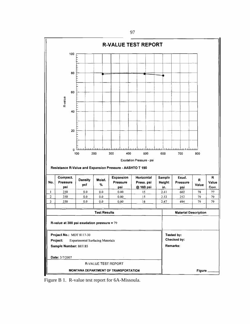
97

Figure B 1. R-value test report for 6A-Missoula.

98

Figure B 2. R-value test report for 6A-Glendive.

99

Figure B 3. R-value test report for 6A-Billings.

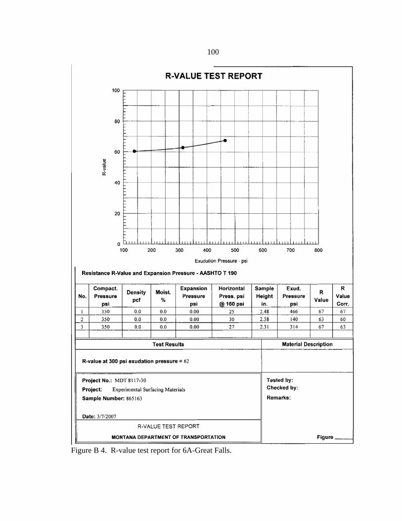
100

Figure B 4. R-value test report for 6A-Great Falls.

101

Figure B 5. R-value test report for 6A-Butte.

102

Figure B 6. R-value test report for 6A-Kalispell.

103


104

Figure B 8. R-value test report for 5A-Kalispell.

105

Figure B 9. R-value test report for 5A-Great Falls.

106

Figure B 10. R-value test report for 2A-Havre.

107

Figure B 11. R-value test report for 2A-Glendive.

108


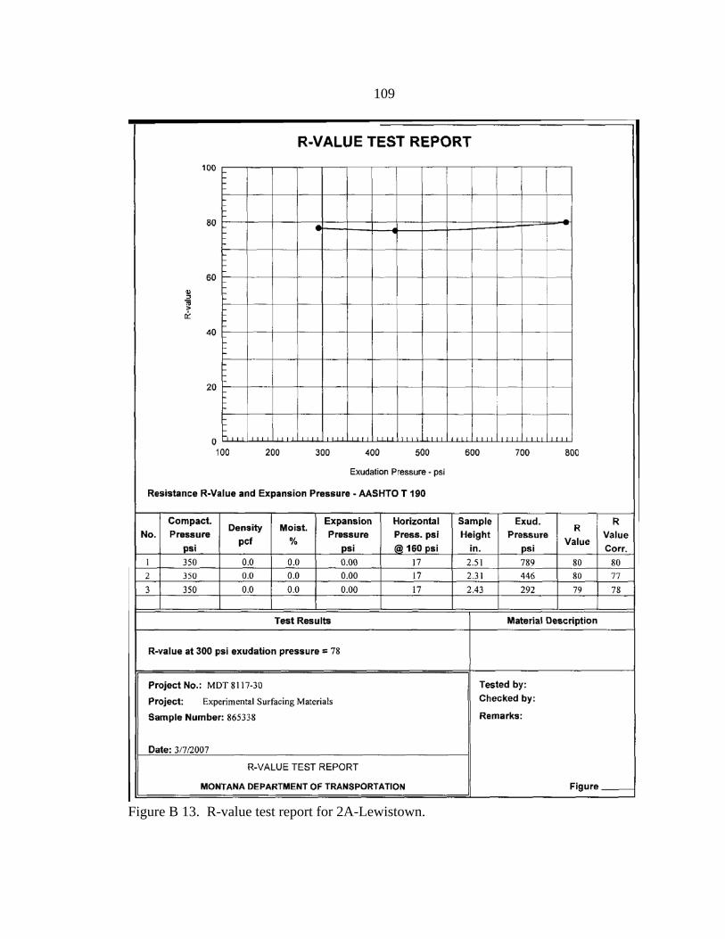
109

Figure B 13. R-value test report for 2A-Lewistown.

110

Figure B 14. R-value test report for 2A-Billings.

111

APPENDIX C

SHEAR STRESS-DISPLACEMENT PLOTS

112

Figure C 1. Shear stress-displacement plots for 5 psi normal stress: a) 6A samples, b) 5A samples, and c) 2A samples.

0

2

4

6

8

10

12

14

16

18

20

0.0 0.5 1.0 1.5 2.0 2.5 3.0 3.5 4.0

Displacement (in)

Shea

r Str

ess

(psi

)

2A Billings, Dr=79.7%2A Glendive, Dr=83.6%2A Lewistown, Dr=86.7%2A Havre, Dr=84.8%2A Missoula, Dr=84.6%

0

2

4

6

8

10

12

14

16

18

20

0.0 0.5 1.0 1.5 2.0 2.5 3.0 3.5 4.0Displacement (in)

Shea

r Str

ess

(psi

)

6A Billings, Dr=64.6%6A Glendive, Dr=65.0%6A Missoula, Dr=65.1%6A Butte, Dr=59.4%6A Great Falls, Dr=62.0%6A Kalispell, Dr=74.5%

0

2

4

6

8

10

12

14

16

18

20

0.0 0.5 1.0 1.5 2.0 2.5 3.0 3.5 4.0Displacement (in)

Shea

r Str

ess

(psi

)

5A Missoula, Dr=75.6%5A Great Falls, Dr=66.6%5A Kalispell, Dr=70.8%

a)

b)

c)

113


0

5

10

15

20

25

30

35

0.0 0.5 1.0 1.5 2.0 2.5 3.0 3.5 4.0Displacement (in)

Shea

r Str

ess

(psi

)


0

5

10

15

20

25

30

35

0.0 0.5 1.0 1.5 2.0 2.5 3.0 3.5 4.0Displacement (in)

Shea

r Str

ess

(psi

)


0

5

10

15

20

25

30

35

0.0 0.5 1.0 1.5 2.0 2.5 3.0 3.5 4.0

Displacement (in)

Shea

r Str

ess

(psi

)


a)

b)

c)

114


0

5

10

15

20

25

30

35

40

0.0 0.5 1.0 1.5 2.0 2.5 3.0 3.5 4.0Displacement (in)

Shea

r Str

ess

(psi

)


0

5

10

15

20

25

30

35

40

0.0 0.5 1.0 1.5 2.0 2.5 3.0 3.5 4.0Displacement (in)

Shea

r Str

ess

(psi

)


0

5

10

15

20

25

30

35

40

0.0 0.5 1.0 1.5 2.0 2.5 3.0 3.5 4.0Displacement (in)

Shea

r Str

ess

(psi

)


a)

b)

c)

115

APPENDIX D

DESPECKLED 2D X-RAY CT IMAGES

116

Figure D 1. 6A-Glendive X-ray CT images top (a) to bottom (i) at 9 mm intervals.

a) b) c)

d) e) f)

g) h) i)

117

Figure D 2. 6A-Missoula X-ray CT images top (a) to bottom (i) at 9 mm intervals.

a) b) c)

d) e) f)

g) h) i)

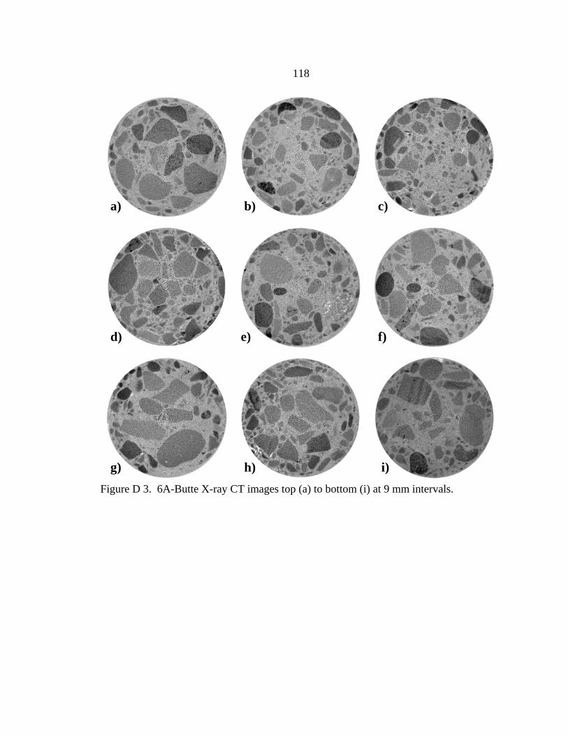
118

Figure D 3. 6A-Butte X-ray CT images top (a) to bottom (i) at 9 mm intervals.

a) b) c)

d) e) f)

g) h) i)

119

Figure D 4. 6A-Kalispell X-ray CT images top (a) to bottom (i) at 9 mm intervals.

a) b) c)

d) e) f)

g) h) i)

120


a) b) c)

d) e) f)

g) h) i)

121

Figure D 6. 5A-Great Falls X-ray CT images top (a) to bottom (i) at 9 mm intervals.

a) b) c)

d) e) f)

g) h) i)

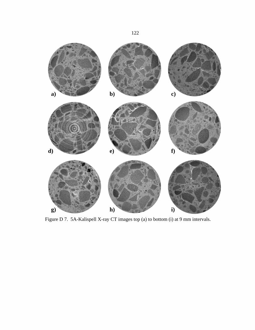
122

Figure D 7. 5A-Kalispell X-ray CT images top (a) to bottom (i) at 9 mm intervals.

a) b) c)

i)h)g)

f)e)d)

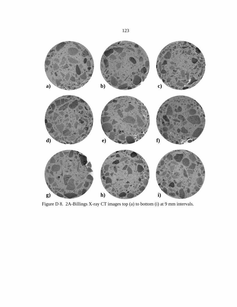
123

Figure D 8. 2A-Billings X-ray CT images top (a) to bottom (i) at 9 mm intervals.

a) b) c)

d) e) f)

g) h) i)

124

Figure D 9. 2A-Glendive X-ray CT images top (a) to bottom (i) at 9 mm intervals.

a) b) c)

d) e) f)

g) h) i)

125

Figure D 10. 2A-Lewistown X-ray CT images top (a) to bottom (i) at 9 mm intervals.

a) b) c)

d) e) f)

g) h) i)

126

Figure D 11. 2A-Havre X-ray CT images top (a) to bottom (i) at 9 mm intervals.

a) b) c)

d) e) f)

g) h) i)

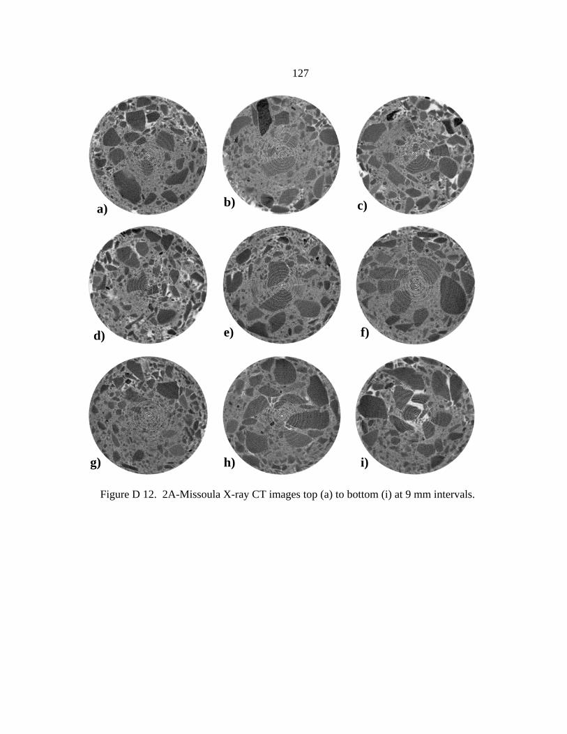
127


a) b) c)

d) e) f)

g) h) i)

128

APPENDIX E

X-RAY CT GRAIN SIZE PLOTS

129

Figure E 1. X-ray CT Derived Grain Size Distributions for CBC-6A Samples: a) Glendive, b) Missoula, c) Butte, and d) Kalispell.


Per

cent

Pas

sing

0

20

40

60

80

100

Sieve dataCT data

50 mm = 1.97 in

a)


Per

cent

Pas

sing

0

20

40

60

80

100

Sieve dataCT data

50 mm = 1.97 in

b)


Per

cent

Pas

sing

0

20

40

60

80

100

Sieve dataCT data

50 mm = 1.97 in

c)


Per

cent

Pas

sing

0

20

40

60

80

100

Sieve dataCT data

50 mm = 1.97 in

d)

130

Figure E 2. X-ray CT Derived Grain Size Distributions for CBC-5A Samples: a) Missoula, b) Great Falls, and c) Kalispell.


Per

cent

Pas

sing

0

20

40

60

80

100

Sieve dataCT data

50 mm = 1.97 in

a)


Per

cent

Pas

sing

0

20

40

60

80

100

Sieve dataCT data

50 mm = 1.97 in

b)


Per

cent

Pas

sing

0

20

40

60

80

100

Sieve dataCT data

50 mm = 1.97 in

c)

131

Figure E 3. X-ray CT Derived Grain Size Distributions for CTS-2A Samples: a) Billings, b) Glendive, c) Lewistown, d) Havre, and e) Missoula.


Per

cent

Pas

sing

0

20

40

60

80

100

Sieve dataCT data

50 mm = 1.97 in

a)


Per

cent

Pas

sing

0

20

40

60

80

100

Sieve dataCT data

50 mm = 1.97 in

b)


Per

cent

Pas

sing

0

20

40

60

80

100

Sieve dataCT data

50 mm = 1.97 in

c)


Per

cent

Pas

sing

0

20

40

60

80

100

Sieve dataCT data

50 mm = 1.97 in

d)


Per

cent

Pas

sing

0

20

40

60

80

100

Sieve dataCT data

50 mm = 1.97 in

e)

Documents

EXPERIMENTAL ASSESSMENT OF AGGREGATES by A thesis