Optics Communications 253 (2005) 109–117

www.elsevier.com/locate/optcom

Experimental and theoretical analysis of leaky extraordinarymodes in negative uniaxial channel waveguides

Giovanni Tartarini a,*, Ralf Stolte b, Hagen Renner c

a Dipartimento di Elettronica, Informatica e Sistemistica, Universita di Bologna, Viale Risorgimento 2, 40136 Bologna, Italyb Adaptif Photonics GmbH, Harburger Schlossstrasse 6-12, D-21079 Hamburg, Germany

c Technische Universitaet Hamburg-Harburg, 2-03 Optische Kommunikationstechnik, Eissendorfer Strasse 40,

D-21073 Hamburg, Germany

Received 2 December 2004; received in revised form 4 April 2005; accepted 21 April 2005

Abstract

We perform a theoretical and experimental study of the radiation losses of extraordinary-like leaky modes in neg-

ative uniaxial waveguides, such as Ti:LiNbO3 channel waveguides, with the axis inclined to the optical axis. Different

waveguides have been realized and characterized varying some fabrication parameters. The numerical model utilized is

based on the assumpton that the leaking power is radiated only by the ordinary substrate field. The comparison

between experimental data and numerical results obtained with this assumption confirms the validity of the approach.

� 2005 Elsevier B.V. All rights reserved.

PACS: 42.82.Et; 42.82.Bq

Keywords: Leaky modes; Anisotropic waveguides; Finite element method; Boundary conditions

1. Introduction

Many anisotropic materials (LiNbO3, LiTaO3,

etc.), exhibit interesting characteristics like piezo-

electric, acousto-optic and non-linear properties,

Therefore, they are widely used for the realization

0030-4018/$ - see front matter � 2005 Elsevier B.V. All rights reserv

doi:10.1016/j.optcom.2005.04.059

* Corresponding author. Tel.: +39 051 2093051; fax: +39 051

2093053.

E-mail address: gtartarini@deis.unibo.it (G. Tartarini).

of a great variety of telecommunication compo-

nents and sensors.

Making an appropriate choice for the orientation

of the crystal axes of these materials at the design

stage [1,2], it is possible to increase the performances

of many devices, like surface acoustic wave (SAW)

components [3], electrooptic polarization convert-ers [4], and directional couplers [5].

However, the anisotropy of the material on

which the electromagnetic field propagates is often

ed.

110 G. Tartarini et al. / Optics Communications 253 (2005) 109–117

connected to the possible presence of leaky modes.

These modes generally cause undesired radiation

losses, and can depend on parameters like the

dimensions of the waveguiding structures [6] or

the orientation of the crystal axes of the aniso-tropic material [7].

When devices based on particular configura-

tions of anisotropic materials are investigated, it

is therefore important to have at disposal an

appropriate modelling tool that is able to predict

the possible presence of leaky modes and the cor-

responding value of leakage losses. Incidentally,

this modelling tool would be able to study as aparticular case also the behaviour of the leaky

modes of important isotropic structures, like AR-

ROW waveguides [8] or photonic crystal fibers [9].

For the calculation of the leakage losses, exact

models [10–12] and approximating analytical for-

mulas [13] have been developed for infinitely

extending anisotropic planar waveguides. How-

ever, practical channel waveguides are confinedto a certain finite cross section, and the numerical

analysis becomes much more complicated. In [14],

it is proposed a method, based on the solution of a

system of integro-differential equations, which can

be successfully applied to the study of leaky modes

in anisotropic channel waveguides exhibiting a

diagonal permittivity tensor.

If anisotropic channel waveguides with non-diagonal permittivity tensor have to be studied,

the finite-element method (FEM) is certainly

among the most versatile tools [16,17].

The FEM calculation of leaky modes of inte-

grated-optical anisotropic channel waveguides

with non-diagonal permittivity tensor has been re-

ported in [18], where the analysis was limited to the

case where the optical axis of the anisotropic mate-rial lies in the plane perpendicular to the wave-

guide axis. In this case, the authors based their

model on the assumption that the structure to be

analyzed is imbedded in an isotropic material, in

order to avoid the introduction of more compli-

cated radiating boundary conditions for aniso-

tropic materials.

With respect to the well-known perfectlymatched layers (PML) boundary conditions [19–

21], this model has the advantage of a potentially

lower cost in terms of CPU memory, since no

additional lossy regions are necessary in the outer

part of the computational domain. In fact, the

hypothesis of an isotropic surrounding medium re-

sults simply in the proper calculation of a line inte-

gral over the boundary of the domain itself.In [22,23], the model proposed in [18] has been

extended for analyzing the important case of leak-

age of the extraordinary leaky mode in anisotropic

waveguides with the waveguide axis not perpendic-

ular to the optical axis [24–26]. Due to the absence

of analytical models describing leaky modes in

two-dimensional (2D) structures, the method was

tested in [23] analyzing 2D structures highly ex-tended along the horizontal direction and compar-

ing the numerical results with rigorously calculated

ones referred to planar structures. In this work, the

validation of the model is further assessed, since

numerical results referring to Ti:LiNbO3 channel

waveguides will be compared with other numerical

results obtained applying the above-mentioned

method [14] and with measured results referredto fabricated waveguides.

In the following, after a brief description of the

model utilized, a numerical comparison will be

presented between the results obtained with our

method and the results presented in [14,15]. Subse-

quently, results coming from experimental mea-

surements performed on real waveguides will be

presented and successfully compared with numeri-cal results computed with our method. Finally,

conclusions will be drawn.

2. Theoretical model

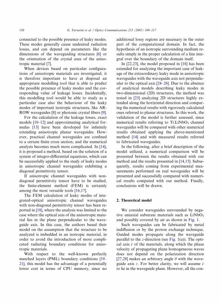
We consider waveguides surrounded by nega-

tive uniaxial substrate materials such as LiNbO3

and possibly covered by air as shown in Fig. 1.

Such waveguides can be fabricated by metal

indiffusion or by the proton exchange technique.

Guided modes propagate along the waveguide

parallel to the z-direction (see Fig. 1(a)). The opti-

cal axis c of the materials, along which the phase

velocity of propagating plane homogeneous waves

does not depend on the polarization direction[27,28] makes an arbitrary angle h with the wave-

guide axis z. For better clarity, we will assume cto lie in the waveguide plane. However, all the con-

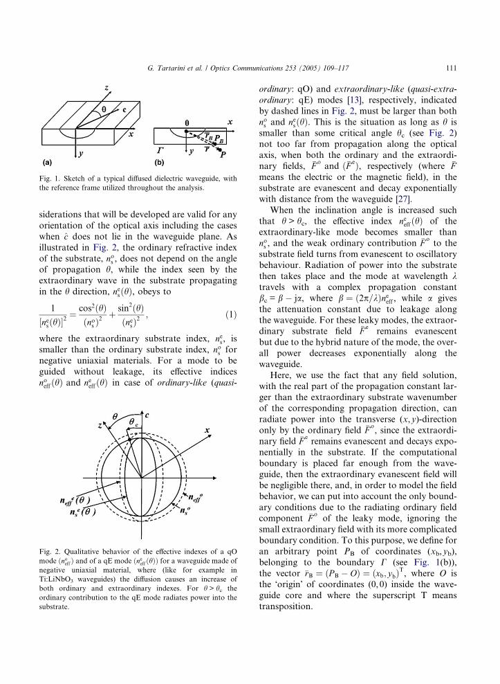
Fig. 1. Sketch of a typical diffused dielectric waveguide, with

the reference frame utilized throughout the analysis.

G. Tartarini et al. / Optics Communications 253 (2005) 109–117 111

siderations that will be developed are valid for any

orientation of the optical axis including the cases

when c does not lie in the waveguide plane. As

illustrated in Fig. 2, the ordinary refractive index

of the substrate, nos , does not depend on the angleof propagation h, while the index seen by the

extraordinary wave in the substrate propagating

in the h direction, nesðhÞ, obeys to

1

½nesðhÞ�2¼ cos2ðhÞ

ðnos Þ2

þ sin2ðhÞðnesÞ

2; ð1Þ

where the extraordinary substrate index, nes , is

smaller than the ordinary substrate index, nos for

negative uniaxial materials. For a mode to be

guided without leakage, its effective indices

noeffðhÞ and neeffðhÞ in case of ordinary-like (quasi-

Fig. 2. Qualitative behavior of the effective indexes of a qO

mode ðnoeffÞ and of a qE mode ðneeffðhÞÞ for a waveguide made of

negative uniaxial material, where (like for example in

Ti:LiNbO3 waveguides) the diffusion causes an increase of

both ordinary and extraordinary indexes. For h > hc the

ordinary contribution to the qE mode radiates power into the

substrate.

ordinary: qO) and extraordinary-like (quasi-extra-

ordinary: qE) modes [13], respectively, indicated

by dashed lines in Fig. 2, must be larger than both

nos and nesðhÞ. This is the situation as long as h is

smaller than some critical angle hc (see Fig. 2)not too far from propagation along the optical

axis, when both the ordinary and the extraordi-

nary fields, �F oand ð�F eÞ, respectively (where �F

means the electric or the magnetic field), in the

substrate are evanescent and decay exponentially

with distance from the waveguide [27].

When the inclination angle is increased such

that h > hc, the effective index neeffðhÞ of theextraordinary-like mode becomes smaller than

nos , and the weak ordinary contribution �F oto the

substrate field turns from evanescent to oscillatory

behaviour. Radiation of power into the substrate

then takes place and the mode at wavelength ktravels with a complex propagation constant

bc = b � ja, where b ¼ ð2p=kÞneeff , while a gives

the attenuation constant due to leakage alongthe waveguide. For these leaky modes, the extraor-

dinary substrate field �F eremains evanescent

but due to the hybrid nature of the mode, the over-

all power decreases exponentially along the

waveguide.

Here, we use the fact that any field solution,

with the real part of the propagation constant lar-

ger than the extraordinary substrate wavenumberof the corresponding propagation direction, can

radiate power into the transverse (x,y)-direction

only by the ordinary field �F o, since the extraordi-

nary field �F eremains evanescent and decays expo-

nentially in the substrate. If the computational

boundary is placed far enough from the wave-

guide, then the extraordinary evanescent field will

be negligible there, and, in order to model the fieldbehavior, we can put into account the only bound-

ary conditions due to the radiating ordinary field

component �F oof the leaky mode, ignoring the

small extraordinary field with its more complicated

boundary condition. To this purpose, we define for

an arbitrary point PB of coordinates (xb,yb),

belonging to the boundary C (see Fig. 1(b)),

the vector �rB ¼ ðPB � OÞ ¼ ðxb; ybÞT, where O is

the �origin� of coordinates (0,0) inside the wave-

guide core and where the superscript T means

transposition.

112 G. Tartarini et al. / Optics Communications 253 (2005) 109–117

With the assumptions taken, the total field �F in

the point P of coordinates (x,y) close to PB (see

again Fig. 1(b)) can be written in its asymptotic

form as

�F ð�rÞ ’ �F oðrBÞrBr

� �1=2

exp½�ikot ðr � rBÞ�

þO jkot rj�3=2

� �ð2Þ

and behaves locally as a plane ordinary wave. In

Eq. (2), rB ¼ j�rBj ¼ffiffiffiffiffiffiffiffiffiffiffiffiffiffiffix2b þ y2b

p;�r ¼ ðP � OÞ ¼ ðx; yÞT

and r ¼ j�rj ¼ffiffiffiffiffiffiffiffiffiffiffiffiffiffix2 þ y2

p.

Generally, the complex number kot , which is re-

lated to the transverse wavevector �ko

t by

�ko

t ¼kotrB

xByB

� �ð3Þ

depends only on the ordinary index nos of the sub-

strate at the boundary point (xB,yB) as

kot ¼ ½k2ðnos Þ2 � b2

c �1=2

, but not on the direction of

rB. Around the point (xB,yB), the slight wavefront

curvature and the asymptotic r�1/2 weakening of

the field due to the cylindrical geometry can be ne-glected against the exponential variation, since its

first derivative is small of order 1=jkot rj � 1 and

can be discarded in the further calculations at this

level of approximation.

The above formulation allows us to calculate

differential expressions of the fields appearing in

the line integrals of the various FEM along the

boundary of the computational window, which re-quire a knowledge of the spatial variation of the

field and hence are responsible for incorporating

the boundary conditions

We applied this formalism in [22,23] to propose

a full-fectorial H-field FEM in the b-formulation

able to model the electromagnetic behavior of lea-

ky modes in anisotropic channel waveguides. As

mentioned in Section 1, the method could be theo-retically tested only referring to 1D planar aniso-

tropic structures, for which rigorous numerical

solutions can be calculated. In the following

sections, this modelling program will be furtherly

validated in the 2D case through the comparison

with numerical results, obtained with a different

method, referring to channel waveguides with

diagonal permittivity tensor, and with experimen-tal results coming from the characterization of real

Ti:LiNbO3 channel waveguides exhibiting a non-

diagonal permittivity tensor.

3. Numerical results

As a theoretical check, our method has been

utilized to calculate the propagation characteristics

of leaky modes in LiNbO3 channel waveguides like

the ones described in [14,15], in order to perform a

comparison.

The ordinary and extraordinary indexes (no and

ne, respectively,) of the waveguides are assumed tofollow the behavior,

no;e ¼ffiffiffiffiffiffiffiffiffiffiffiffiffiffiffiffiffiffiffiffiffiffiffiffiffiffiffiffiffiffiffiffiffiffiffiffiffiffiffiffiffiðno;es Þ2 þ Def ðyÞgðxÞ

q. ð4Þ

In Eq. (4), it is nos ¼ffiffiffiffiffiffiffi5.2

p; nes ¼

ffiffiffiffiffiffiffiffiffi4.84

p, while

f ðyÞ ¼ e�ðy=DÞ2 ; and

gðxÞ ¼ 0.5 � erfxþ 0.5W

D

� �� erf

x� 0.5WD

� �� .

It is assumed that W = 2D, and it is also assumedthat the quantity V ¼ ð2p=kÞD

ffiffiffiffiffiffiDe

phas the value

V = 3.5. The wavelength utilized is k = .632 lm.

Waveguides obtained with the c-axis along

the vertical direction (Z-cut configuration) and

with the c-axis along the horizontal direction

(X-cut Y-propagation configuration) have been

considered.

For these waveguides, the characteristics of thefundamental qE leaky mode have been calculated

for different values of De (keeping the relationship

V = 3.5).

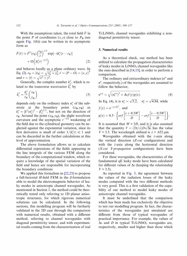
As reported in Fig. 3, the agreement between

the values of the radiation losses of the leaky

modes computed with the two different methods

is very good. This is a first validation of the capa-

bility of our method to model leaky modes ofanisotropic channel waveguides.

It must be underlined that the comparison

which has been made has exclusively the objective

to test our modelling program. In fact, the charac-

teristics of the waveguides just simulated are

different from those of typical waveguides of

practical importance. For example, the values of

De and D in typical Ti:LiNbO3 waveguides are,respectively, smaller and higher than those which

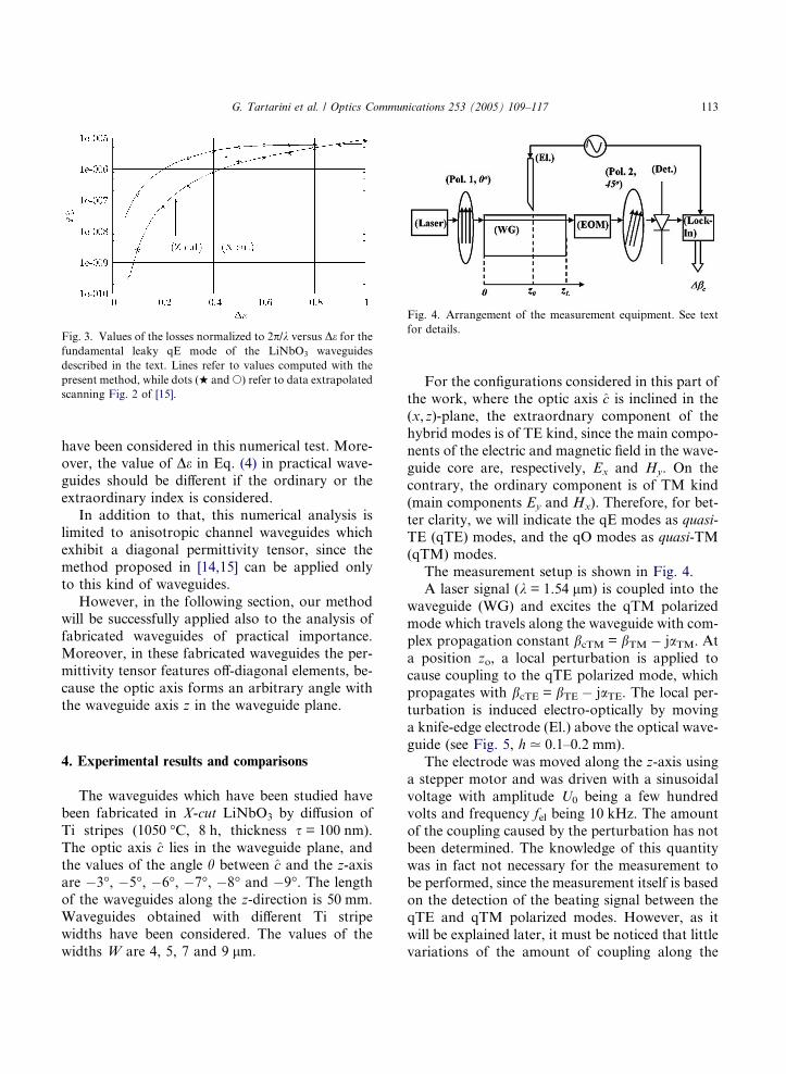
Fig. 4. Arrangement of the measurement equipment. See text

for details.Fig. 3. Values of the losses normalized to 2p/k versus De for thefundamental leaky qE mode of the LiNbO3 waveguides

described in the text. Lines refer to values computed with the

present method, while dots (w ands) refer to data extrapolated

scanning Fig. 2 of [15].

G. Tartarini et al. / Optics Communications 253 (2005) 109–117 113

have been considered in this numerical test. More-

over, the value of De in Eq. (4) in practical wave-guides should be different if the ordinary or the

extraordinary index is considered.

In addition to that, this numerical analysis is

limited to anisotropic channel waveguides which

exhibit a diagonal permittivity tensor, since the

method proposed in [14,15] can be applied only

to this kind of waveguides.

However, in the following section, our methodwill be successfully applied also to the analysis of

fabricated waveguides of practical importance.

Moreover, in these fabricated waveguides the per-

mittivity tensor features off-diagonal elements, be-

cause the optic axis forms an arbitrary angle with

the waveguide axis z in the waveguide plane.

4. Experimental results and comparisons

The waveguides which have been studied have

been fabricated in X-cut LiNbO3 by diffusion of

Ti stripes (1050 �C, 8 h, thickness s = 100 nm).

The optic axis c lies in the waveguide plane, and

the values of the angle h between c and the z-axis

are �3�, �5�, �6�, �7�, �8� and �9�. The lengthof the waveguides along the z-direction is 50 mm.

Waveguides obtained with different Ti stripe

widths have been considered. The values of the

widths W are 4, 5, 7 and 9 lm.

For the configurations considered in this part ofthe work, where the optic axis c is inclined in the

(x,z)-plane, the extraordnary component of the

hybrid modes is of TE kind, since the main compo-

nents of the electric and magnetic field in the wave-

guide core are, respectively, Ex and Hy. On the

contrary, the ordinary component is of TM kind

(main components Ey and Hx). Therefore, for bet-

ter clarity, we will indicate the qE modes as quasi-TE (qTE) modes, and the qO modes as quasi-TM

(qTM) modes.

The measurement setup is shown in Fig. 4.

A laser signal (k = 1.54 lm) is coupled into the

waveguide (WG) and excites the qTM polarized

mode which travels along the waveguide with com-

plex propagation constant bcTM = bTM � jaTM. At

a position zo, a local perturbation is applied tocause coupling to the qTE polarized mode, which

propagates with bcTE = bTE � jaTE. The local per-

turbation is induced electro-optically by moving

a knife-edge electrode (El.) above the optical wave-

guide (see Fig. 5, h . 0.1–0.2 mm).

The electrode was moved along the z-axis using

a stepper motor and was driven with a sinusoidal

voltage with amplitude U0 being a few hundredvolts and frequency fel being 10 kHz. The amount

of the coupling caused by the perturbation has not

been determined. The knowledge of this quantity

was in fact not necessary for the measurement to

be performed, since the measurement itself is based

on the detection of the beating signal between the

qTE and qTM polarized modes. However, as it

will be explained later, it must be noticed that littlevariations of the amount of coupling along the

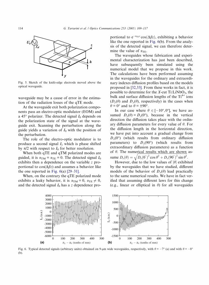
Fig. 5. Sketch of the knife-edge electrode moved above the

optical waveguide.

114 G. Tartarini et al. / Optics Communications 253 (2005) 109–117

waveguide may be a cause of error in the estima-tion of the radiation losses of the qTE mode.

At the waveguide exit both polarization compo-

nents pass an electro-optic modulator (EOM) and

a 45� polarizer. The detected signal I0 depends on

the polarization state of the signal at the wave-

guide exit. Scanning the perturbation along the

guide yields a variation of I0 with the position of

the perturbation.The role of the electro-optic modulator is to

produce a second signal I1 which is phase shifted

by p/2 with respect to I0 for better resolution.

When both qTE and qTM polarized modes are

guided, it is aTM = aTE = 0. The detected signal I0exhibits then a dependence on the variable z pro-

portional to cos(Dbz) and assumes a behavior like

the one reported in Fig. 6(a) [29–31].When, on the contrary the qTE polarized mode

exhibits a leaky behavior, it is aTM = 0, aTE 6¼ 0,

and the detected signal I0 has a z dependence pro-

(a) (b

Fig. 6. Typical detected signals (arbitrary units) obtained on 9-lm w

(b).

portional to e�aTEz cosðDbzÞ, exhibiting a behavior

like the one reported in Fig. 6(b). From the analy-

sis of the detected signal, we can therefore deter-

mine the value of aTE.The waveguides whose fabrication and experi-

mental characterization has just been described,

have subsequently been simulated using the

numerical model that we propose in this work.

The calculations have been performed assuming

in the waveguides for the ordinary and extraordi-

nary indexes diffusion profiles based on the models

proposed in [32,33]. From these works in fact, it is

possible to determine for the X-cut Ti:LiNbO3, thebulk and surface diffusion lengths of the Ti4+ ions

(Dy(h) and Dx(h), respectively) in the cases when

h = 0� and to h = ±90�.In our case where h 2 [�10�, 0�], we have as-

sumed Dy(h) = Dy(0�), because in the vertical

direction the diffusion takes place with the ordin-

ary diffusion parameters for every value of h. Forthe diffusion length in the horizontal direction,we have put into account a gradual change from

Dx(0�) (which results from ordinary diffusion

parameters) to Dx(90�) (which results from

extraordinary diffusion parameters) as a function

of h. The numerical results which are shown as-

sume DxðhÞ ¼ffiffiffiffiffiffiffiffiffiffiffiffiffiffiffiffiffiffiffiffiffiffiffiffiffiffiffiffiffiffiffiffiffiffiffiffiffiffiffiffiffiffiffiffiffiffiffiffiffiffiffiffiffiffiffiffiffiffiffiffiffiffiDxð0

� Þ2 cos h2 þ Dxð90� Þ2 sin h2

q.

However, due to the low values of jhj exhibitedby the waveguides that we have studied, different

models of the behavior of Dx(h) lead practicallyto the same numerical results. We have in fact ver-

ified that assuming different laws for this change

(e.g., linear or elliptical in h) for all waveguides

)

ide waveguides, respectively, with h = �7� (a) and with h = �8�

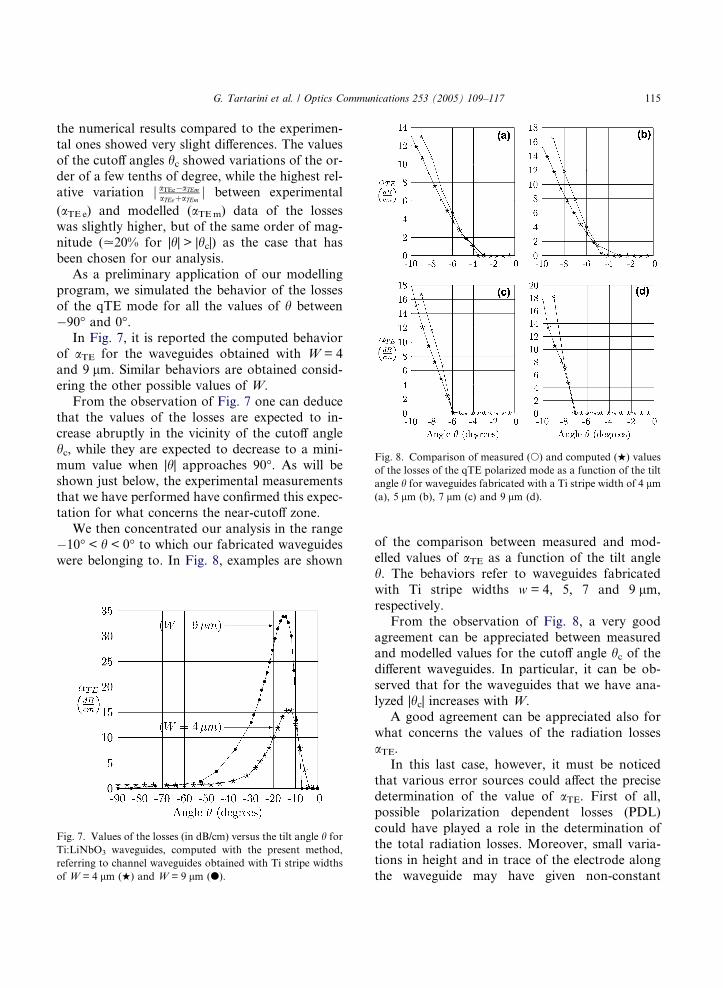
Fig. 8. Comparison of measured (s) and computed (w) values

of the losses of the qTE polarized mode as a function of the tilt

angle h for waveguides fabricated with a Ti stripe width of 4 lm(a), 5 lm (b), 7 lm (c) and 9 lm (d).

G. Tartarini et al. / Optics Communications 253 (2005) 109–117 115

the numerical results compared to the experimen-

tal ones showed very slight differences. The values

of the cutoff angles hc showed variations of the or-

der of a few tenths of degree, while the highest rel-

ative variation j aTEe�aTEmaTEeþaTEm

j between experimental

(aTEe) and modelled (aTEm) data of the losseswas slightly higher, but of the same order of mag-

nitude (.20% for |h| > |hc|) as the case that has

been chosen for our analysis.

As a preliminary application of our modelling

program, we simulated the behavior of the losses

of the qTE mode for all the values of h between

�90� and 0�.In Fig. 7, it is reported the computed behavior

of aTE for the waveguides obtained with W = 4

and 9 lm. Similar behaviors are obtained consid-

ering the other possible values of W.

From the observation of Fig. 7 one can deduce

that the values of the losses are expected to in-

crease abruptly in the vicinity of the cutoff angle

hc, while they are expected to decrease to a mini-

mum value when |h| approaches 90�. As will beshown just below, the experimental measurements

that we have performed have confirmed this expec-

tation for what concerns the near-cutoff zone.

We then concentrated our analysis in the range

�10� < h < 0� to which our fabricated waveguides

were belonging to. In Fig. 8, examples are shown

Fig. 7. Values of the losses (in dB/cm) versus the tilt angle h for

Ti:LiNbO3 waveguides, computed with the present method,

referring to channel waveguides obtained with Ti stripe widths

of W = 4 lm (w) and W = 9 lm (d).

of the comparison between measured and mod-

elled values of aTE as a function of the tilt angle

h. The behaviors refer to waveguides fabricated

with Ti stripe widths w = 4, 5, 7 and 9 lm,

respectively.

From the observation of Fig. 8, a very good

agreement can be appreciated between measuredand modelled values for the cutoff angle hc of thedifferent waveguides. In particular, it can be ob-

served that for the waveguides that we have ana-

lyzed |hc| increases with W.

A good agreement can be appreciated also for

what concerns the values of the radiation losses

aTE.In this last case, however, it must be noticed

that various error sources could affect the precise

determination of the value of aTE. First of all,

possible polarization dependent losses (PDL)

could have played a role in the determination of

the total radiation losses. Moreover, small varia-

tions in height and in trace of the electrode along

the waveguide may have given non-constant

116 G. Tartarini et al. / Optics Communications 253 (2005) 109–117

coupling conditions between the two polariza-

tions. This is, in effect, the origin of the non-con-

stant envelope in the measurement curve reported

in Fig. 6(a).

Finally, the leaky field which is present in thebulk part of the waveguide substrate can have

interacted with the signal at the detector. We be-

lieve for example that this can be the origin of

the asymmetric response around the zero value in

Fig. 6(b).

As for the PDL, since the two polarization

modes have about similar losses, which in this case

can be expected to be a few tenths of a dB, we con-cluded that we could neglect their effect here, be-

cause it is well below the leaking effect that we

were looking for in this work. About the other

possible causes of error in the determination of

the value of aTE, we did not perform a detailed er-

ror analyisis. The values of aTE that we have ob-

tained must then be seen as approximate values,

which can give us an idea of the amount of radia-tion losses which the qTE modes undergo once

|h| < |hc|.The comparisons reported in Fig. 8 show, there-

fore, that the theoretical model that we have uti-

lized is able to compute the value of the cutoff

angle hc, and, at least on an order-of-magnitude

basis, the values of aTE of the leaky modes of

anisotropic channel waveguides.

5. Conclusions

Through the comparison between calculated

and experimentally measured results, we have

tested a theoretical model to study with the finite

element method the characteristics of leakymodes in anisotropic channel waveguides. The

model is based on the assumption that, suffi-

ciently far from the waveguide core, only the or-

dinary component of the modes can be assumed

to be present without altering the field character-

istics. The good agreement between theoretical

and experimental results confirms the correctness

of the proposed approach. The model developedcan, therefore, become a useful tool at the design

stage for the fabrication of some important IO

devices.

Acknowledgements

The authors thank Paolo Bassi for helpful

discussions. This work has been supported by the

Italian Ministry of University and Education.

References

[1] W. Yue, J. Yi-Jian, Opt. Mater. 23 (2003) 403.

[2] N. Naumeno, B. Abbott, IEEE Symp. Ultrasonics 2 (2003)

2110.

[3] F. Martin, M.I. Newton, G. McHale, K.A. Melzak, E.

Gizeli, Biosens. BioElectron. 19 (2003) 627.

[4] T. Wang, J. Chung, IEEE Photonics Technol. Lett. 16

(2004) 2275.

[5] M. Tounsi, A. Khodja, B. Haraoubia, in: IEEE Interna-

tional Conference on Electronics, Circuits and Systems,

ICECS 2003, vol. 3, 2003, p. 966.

[6] T. Hashimoto, Y. Kobayashi, IEEE MTT-S Int. 3 (2002)

1975.

[7] P. Wallner, W. Ruile, R. Weigel, IEEE Trans. Ultrason.

Ferr. 47 (2000) 1235.

[8] C.W. Tee, S.F. Yu, N.S. Chen, IEEE J. Lightwave

Technol. 22 (2004) 1797.

[9] D. Ferrarini, L. Vincetti, M. Zoboli, A. Cucinotta, F. Poli,

S. Selleri, in: Proceedings of Optical Fiber Communica-

tions Conference, OFC 2003, 2003, p. 699.

[10] G. Tartarini, P. Bassi, P. Baldi, M.P. De Micheli, D.B.

Ostrowsky, Appl. Opt. 34 (1995) 3441.

[11] I. Avrutsky, J. Opt. Soc., Am. 20 (2003) 548.

[12] H.P. Uranus, H.J.W.M. Hoekstra, E. Van Groesen, Opt.

Quant. Electron. 36 (2004) 239.

[13] S.K. Sheem, W.K. Burns, A.F. Milton, Opt. Lett. 3 (1978)

76.

[14] A.B. Sotsky, L.I. Sotskaya, Opt. Quant. Electron. 31

(1999) 733.

[15] A.B. Sotsky, J. Commun. Technol. Electron. 47 (2002)

707.

[16] M. Koshiba, Optical Waveguide Theory by the Finite

Element Method, KTK Scientific Publishers, Tokyo,

1992.

[17] F.A. Fernandez, Y. Lu, Microwave and Optical Wave-

guide Analysis by the Finite Element Method, Research

Studies Press, Taunton, 1996.

[18] H.E. Hernandez-Figueroa, F.A. Fernandez, Y. Lu, J.B.

Davies, IEEE Trans. Magnet. 31 (1995) 1710.

[19] Z.S. Sacks, D.M. Kingsland, R. Lee, Jin-Fa Lee, IEEE

Trans. Antennas Prop. 43 (1995) 1460.

[20] S. Selleri, L. Vincetti, A. Cucinotta, D.M. Zoboli, Opt.

Quant. Electron. 33 (2001) 359.

[21] S.S.A. Obayya, B.M.A. Rahman, K.T.V. Grattan, H.A.

El-Mikati, J. Lightwave Technol. 20 (2002) 1054.

[22] G. Tartarini, H. Renner, IEEE Microw. Guided Wave

Lett. 9 (1999) 389.

G. Tartarini et al. / Optics Communications 253 (2005) 109–117 117

[23] G. Tartarini, Opt. Quant. Electron. 32 (2000) 719.

[24] S. Bahndare, R. Noe, in: 10th European Conference on

Integrated Optics, ECIO 2001, Paderborn, Germany, April

4–6, 2001, p. 172.

[25] S. Sonoda, I. Tsuruma, M. Hatori, Appl. Phys. Lett. 71

(1997) 3048.

[26] R. Stolte, R. Ulrich, Electron. Lett. 33 (1997) 1217.

[27] D.P.GiaRusso, J.H.Harris, J. Opt. Soc., Am. 63 (1973) 138.

[28] A. Yariv, P. Yeh, Optical Waves in Crystals, Wiley, New

York, 1984.

[29] R. Stolte, R. Ulrich, Opt. Lett. 20 (2) (1995) 142.

[30] R. Stolte, R. Ulrich, Electron. Lett. 32 (1996) 814.

[31] Reinhard Ulrich, Ralf Stolte, Harald Gnewuch, Giovanni

Tartarini, in: Proceedings of Cleo-Europe �96, Hamburg,

Germany, 1996.

[32] E. Strake, G.P. Bava, I. Montrosset, IEEE J. Lightwave

Technol. 6 (1988) 1126.

[33] S. Fouchet, A. Carenco, C. Dauget, R. Guglielmi,

L. Riviere, IEEE J. Lightwave Technol. 5 (1987)

700.