Embed Size (px)
Citation preview
EXPERIMENTAL AND NUMERICAL STUDY
OF
SPRING-IN ANGLE IN CORNER SHAPED COMPOSITE PARTS
A THESIS SUBMITTED TO
THE GRADUATE SCHOOL OF NATURAL AND APPLIED SCIENCES
OF
MIDDLE EAST TECHNICAL UNIVERSITY
BY
KEREM FURKAN ÇİÇEK
IN PARTIAL FULLFILLMENT OF THE REQUIREMENTS
FOR
THE DEGREE OF MASTER OF SCIENCE
IN
MECHANICAL ENGINEERING
SEPTEMBER 2014

Approval of the thesis:
EXPERIMENTAL AND NUMERICAL STUDY
OF
SPRING-IN ANGLE IN CORNER SHAPED COMPOSITE PARTS
submitted by KEREM FURKAN ÇİÇEK in partial fulfillment of the requirements
for the degree of Master of Science in Mechanical Engineering Department,
Middle East Technical University by,
Prof. Dr. Canan Özgen
Dean, Graduate School of Natural and Applied Sciences
Prof. Dr. Süha Oral
Head of Department, Mechanical Engineering
Assist. Prof. Dr. Merve Erdal
Supervisor, Mechanical Engineering Dept., METU
Prof. Dr. Altan Kayran
Co-Supervisor, Aerospace Engineering Dept., METU
Examining Committee Members:
Prof. Dr. Haluk Darendeliler
Mechanical Engineering Dept., METU
Assist. Prof. Dr. Merve Erdal
Mechanical Engineering Dept., METU
Prof. Dr. Altan Kayran
Aerospace Engineering Dept., METU
Prof. Dr. Levend Parnas
Mechanical Engineering Dept., METU
Prof. Dr. Serkan Dağ
Mechanical Engineering Dept., METU
Date: 02/09/2014

iv
I hereby declare that all information in this document has been obtained and
presented in accordance with academic rules and ethical conduct. I also
declare that, as required by these rules and conduct, I have fully cited and
referenced all material and results that are not original to this work.
Name, Last name : Kerem Furkan ÇİÇEK
Signature :
v
ABSTRACT
EXPERIMENTAL AND NUMERICAL STUDY
OF
SPRING-IN ANGLE IN CORNER SHAPED COMPOSITE PARTS
Çiçek, Kerem Furkan
M. S., Department of Mechanical Engineering
Supervisor: Assist. Prof. Dr. Merve Erdal
Co-supervisor: Prof. Dr. Altan Kayran
September 2014, 110 Pages
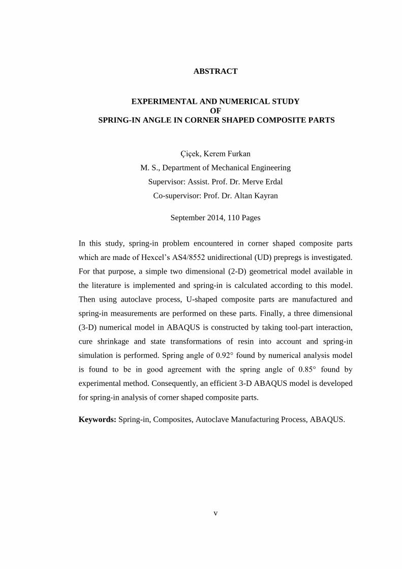
In this study, spring-in problem encountered in corner shaped composite parts
which are made of Hexcel’s AS4/8552 unidirectional (UD) prepregs is investigated.
For that purpose, a simple two dimensional (2-D) geometrical model available in
the literature is implemented and spring-in is calculated according to this model.
Then using autoclave process, U-shaped composite parts are manufactured and
spring-in measurements are performed on these parts. Finally, a three dimensional
(3-D) numerical model in ABAQUS is constructed by taking tool-part interaction,
cure shrinkage and state transformations of resin into account and spring-in
simulation is performed. Spring angle of 0.92° found by numerical analysis model
is found to be in good agreement with the spring angle of 0.85° found by
experimental method. Consequently, an efficient 3-D ABAQUS model is developed
for spring-in analysis of corner shaped composite parts.
Keywords: Spring-in, Composites, Autoclave Manufacturing Process, ABAQUS.
vi
ÖZ
KÖŞELİ GEOMETRİYE SAHİP KOMPOZİT PARÇALARDA OLUŞAN
GERİ YAYLANMANIN DENEYSEL VE NÜMERİK OLARAK
İNCELENMESİ
Çiçek, Kerem Furkan
Yüksek Lisans, Makina Mühendisliği Bölümü,
Tez Yöneticisi: Yard. Doç. Dr. Merve Erdal
Ortak Tez Yöneticisi: Prof. Dr. Altan Kayran
Eylül 2014, 110 Sayfa
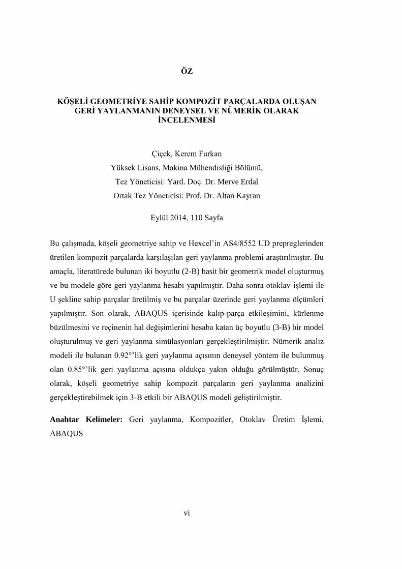
Bu çalışmada, köşeli geometriye sahip ve Hexcel’in AS4/8552 UD prepreglerinden
üretilen kompozit parçalarda karşılaşılan geri yaylanma problemi araştırılmıştır. Bu
amaçla, literatürede bulunan iki boyutlu (2-B) basit bir geometrik model oluşturmuş
ve bu modele göre geri yaylanma hesabı yapılmıştır. Daha sonra otoklav işlemi ile
U şekline sahip parçalar üretilmiş ve bu parçalar üzerinde geri yaylanma ölçümleri
yapılmıştır. Son olarak, ABAQUS içerisinde kalıp-parça etkileşimini, kürlenme
büzülmesini ve reçinenin hal değişimlerini hesaba katan üç boyutlu (3-B) bir model
oluşturulmuş ve geri yaylanma simülasyonları gerçekleştirilmiştir. Nümerik analiz
modeli ile bulunan 0.92°’lik geri yaylanma açısının deneysel yöntem ile bulunmuş
olan 0.85°’lik geri yaylanma açısına oldukça yakın olduğu görülmüştür. Sonuç
olarak, köşeli geometriye sahip kompozit parçaların geri yaylanma analizini
gerçekleştirebilmek için 3-B etkili bir ABAQUS modeli geliştirilmiştir.
Anahtar Kelimeler: Geri yaylanma, Kompozitler, Otoklav Üretim İşlemi,
ABAQUS

vii
To my fiancée and my family,

viii
ACKNOWLEDGEMENTS
I gratefully acknowledge the support and guidance of my thesis advisors Assist.
Prof. Dr. Merve Erdal and Prof. Dr. Altan Kayran. With their thoughtful
encouragement and discreet supervision, I was able to finish my thesis.
I would like to express my sincere gratitude to my supervisors Tahir Fidan and
Suphi Yılmaz, at ASELSAN Inc. for their support and patience throughout my
thesis studies.
I am also grateful to İhsan Otabatmaz from EPSİLON Composite for his
contributions on the experiments I conducted during my thesis. My thanks also go
out to my colleague, Oğuz Doğan, who helped me during ABAQUS modeling.
I extend my sincere thanks to my parents Sevda and Atalay Çiçek for their
encouragement and support in every moment of my life.
Finally, my deepest thanks go to my fiancée, Merve Soyarslan, for her love and
never-ending support.

ix
TABLE OF CONTENTS
ABSTRACT ............................................................................................................... v
ÖZ ............................................................................................................................. vi
ACKNOWLEDGEMENTS .................................................................................... viii
TABLE OF CONTENTS .......................................................................................... ix
LIST OF TABLES ................................................................................................... xii
LIST OF FIGURES................................................................................................. xiii
NOMENCLATURE ............................................................................................... xvii
LIST OF ABBREVIATIONS ............................................................................... xviii
CHAPTERS
1.INTRODUCTION................................................................................................... 1
1.1 COMPOSITE MATERIALS....................................................................... 1
1.1.1 Thermoset Composites ......................................................................... 2
1.1.2 Thermoplastic Composites ................................................................... 3
1.1.3 Fiber Reinforcements ........................................................................... 4
1.1.4 Manufacturing Processes ..................................................................... 7
1.2 MANUFACTURING INDUCED SHAPE DISTORTION PROBLEMS IN
THERMOSET COMPOSITES VIA AUTOCLAVE FORMING PROCESS ..... 13
1.2.1 Vacuum Bagging and Cure Cycle ...................................................... 13
1.2.2 Shape Distortion Problems in Autoclave Forming Process ............... 16
1.3 OBJECTIVE OF THE THESIS ................................................................ 23
1.4 THESIS OUTLINE ................................................................................... 23
2.ANALYTICAL DETERMINATION OF SPRING-IN ........................................ 25
x
2.1 GEOMETRIC DEFINITION OF SPRING-IN ......................................... 25
2.2 3-D EFFECTIVE THERMOMECHANICAL PROPERTIES OF A
SYMMETRIC AND BALANCED LAMINATE ................................................ 29
2.2.1 Effective Stiffness Matrix .................................................................. 29
2.2.2 Effective Coefficient of Thermal Expansions (CTEs) ....................... 36
2.3 EFFECTIVE CURE SHRINKAGE OF A SYMMETRIC AND
BALANCED LAMINATE ................................................................................... 40
2.4 MATERIAL PROPERTIES NEEDED FOR THE CALCULATION OF
SPRING-IN ANGLE ............................................................................................ 42
3.EXPERIMENTAL INVESTIGATION OF SPRING-IN...................................... 45
3.1. LAY-UP CONFIGURATION, MATERIAL TYPE AND DIMENSIONS
45
3.2. AUTOCLAVE FORMING PROCESS ..................................................... 47
3.2.1. Preparing the Tool Surface and Prepregs ........................................... 47
3.2.2. Intermediate Vacuum Bagging Process ............................................. 48
3.2.3. Final Vacuum Bagging Process ......................................................... 49
3.2.4. Thermocouple Installation to a Specific Manufacturing Assembly ... 50
3.2.5. Cure Cycle .......................................................................................... 53
3.2.6. Temperature Field Data Obtained From Thermocoupled
Manufacturing Assembly .................................................................................. 53
3.3. MEASURING THE SPRING-IN ANGLE ............................................... 54
3.3.1. Scanning Mating Surfaces of the Composite and the Tool via Optical
Measuring Device ................................................................................................. 54
3.3.2. Processing Scanned Surfaces in CATIA Environment .......................... 57
4.NUMERICAL ANALYSIS MODEL FOR SPRING-IN SIMULATION ............ 61
xi
4.1. MATERIAL PROPERTIES OF AS4/8552 COMPOSITE SYSTEM AND
ALUMINUM TOOL ............................................................................................ 62
4.2. ABAQUS ANALYSIS MODEL ............................................................... 68
4.2.1. FEM Models in the Literature ............................................................ 68
4.2.2. Modeling Strategy in ABAQUS ........................................................ 71
4.2.3. The Effect of Cure Shrinkage on the Spring-in ................................. 82
4.2.4. The Effect of Tool-part Interaction on Spring-in ............................... 82
5.RESULTS AND DISCUSSIONS ......................................................................... 85
5.1. SPRING-IN ANGLE CALCULATION VIA ANALYTICAL MODEL . 86
5.2. SPRING-IN ANGLE MEASUREMENT VIA EXPERIMENT ............... 87
5.3. SPRING-IN ANGLE CALCULATION VIA NUMERICAL ANALYSIS
MODEL ................................................................................................................ 90
5.4. COMPARISON OF SPRING-IN ANGLES FOUND BY ANALYTICAL
MODEL, EXPERIMENT AND NUMERICAL ANALYSIS MODEL ............ 101
6.CONCLUSIONS ................................................................................................. 103
REFERENCES ....................................................................................................... 105
xii
LIST OF TABLES
Table 1 – Some of the Necessary Material Properties of Hexcel’s AS4/8552
Composite System for Analytical Spring-in Calculation [51] ......................... 44
Table 2 – Some of the Necessary Material Properties of Hexcel’s AS4/8552
Composite System for Spring-in Modeling [51] .............................................. 63
Table 3 – Average thermal conductivities of AS4/8552 used in ABAQUS analysis
model ................................................................................................................ 65
Table 4 – Average specific heat capacities of AS4/8552 used in ABAQUS analysis
model ................................................................................................................ 67
Table 5 – Material properties of aluminum tools (6061 series, T6 heat treatment)
used in ABAQUS analysis model [68]............................................................. 67
Table 6 – Comparison Between Numerical Model Developed in This Thesis and
Çınar’s Numerical Model ................................................................................. 72
Table 7 – Thermal conductance and related clearance values defined in the analysis
model ................................................................................................................ 79
Table 8 – Spring-in angles calculated by using the 2-D analytical model ............... 86
Table 9 – Measured angles, i i an on each composite part ......... 89
Table 10 – Measured angles, i i an on each tool ......................... 89
Table 11 - Spring-in angles, i i an ............................................ 89
Table 12 – Spring-in angles calculated by using different coefficient of friction (μ)
values in primary analysis model ..................................................................... 96
Table 13 – Spring-in angles calculated by each ABAQUS analysis model ........... 101
Table 14 –Comparison of Spring-in Angles Found by Three Different Methods . 102
xiii
LIST OF FIGURES
Figure 1: Schematic of 2-D fiber arrangement [10] ................................................... 4
Figure 2: Comparison of in-plane and through thickness tensile modulus of some
engineering composites having 2-D fiber arrangement [10] .............................. 5
Figure 3: UD continuous 2-D fiber arrangement ....................................................... 5
Figure 4: Crossply or woven fabric 2-D fiber arrangement in a composite ............... 6
Figure 5: 3-D braided para-aramid perform [11] ....................................................... 6
Figure 6: Unidirectional lay-up configuration [12] .................................................... 7
Figure 7: Symmetric and balanced lay-up configuration [14] ................................... 8
Figure 8: Hand lay-up process [12] ............................................................................ 9
Figure 9: RTM process [12] ..................................................................................... 10
Figure 10: Autoclave forming process [16] ............................................................. 11
Figure 11: Schematic view of a UD prepreg [17] .................................................... 12
Figure 12: A typical vacuum bagging process [18] ................................................. 13
Figure 13: Cure cycle for Hexcel’s AS4/8552 UD prepregs [21] ............................ 15
Figure 14: Material behavior of a thermosetting composite during a typical cure
cycle [23] .......................................................................................................... 16
Figure 15: Drapability Simulation in PAM-QUIK FORM [27] .............................. 17
Figure 16: Warpage on an initially flat part [30] ..................................................... 18
Figure 17: Spring-in on a corner section [34] .......................................................... 19
Figure 18: Elimination of tension-shear coupling when a tensile force applied on
balanced laminate [1] ....................................................................................... 21
Figure 19: Warpage Mechanism: a) Tool expansion due to heating of tool up to cure
temperature b) Inter-ply slippage due to stress gradients in the through
thickness direction c) Initially flat part is curved after demolding [31] ........... 23
Figure 20: Change in the enclosed angle of corner section after curing process 26
Figure 21: Cross-section of an L shaped part ........................................................... 28
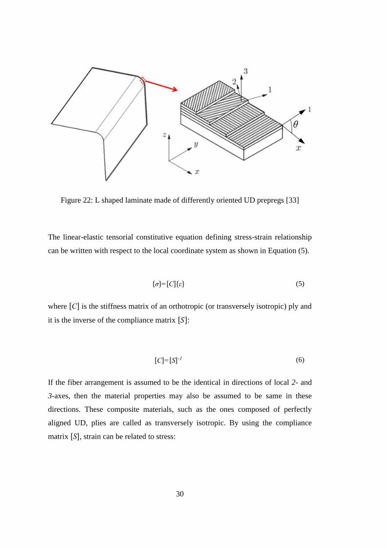
Figure 22: L shaped laminate made of differently oriented UD prepregs [33] ........ 30
xiv
Figure 23: r-θ and x-y-z coordinate systems displayed on the cross section of an L-
shaped part ........................................................................................................ 40
Figure 24: Cure shrinkage strains ( ) and ( ) with the corresponding r-θ
coordinate system displayed on an L-shaped part ............................................ 42
Figure 25: U-shaped composite laminate studied in the thesis ................................ 43
Figure 26: Dimensions of Composite Parts (in mm) ................................................ 46
Figure 27: Dimensions of Tools (in mm) ................................................................. 47
Figure 28: Intermediate vacuum bagging process .................................................... 48
Figure 29: Final Vacuum Bagging Process .............................................................. 49
Figure 30: Vacuum bagged manufacturing assemblies inside the autoclave chamber
.......................................................................................................................... 50
Figure 31: Schematic View of Thermocouple Installation ...................................... 51
Figure 32: Thermocouple codes and their locations ................................................ 52
Figure 33: Temperature vs. Time Graph Showing Each Thermocouple Data ......... 54
Figure 34: Spring-in of a composite part by eye inspection ..................................... 55
Figure 35: Reference markers and the application of gray spray on: a) Composite
Part Surface b) Tool Surface ............................................................................ 56
Figure 36: Scanning Process of the Tool.................................................................. 57
Figure 37: a) Importing the scanned surface of the composite part in .stl format b)
Creating automatic surface from the .stl data ................................................... 58
Figure 38: Deviation analysis performed on newly generated surface with respect to
the scanned data................................................................................................ 58
Figure 39: Angles i i an measured in CATIA for composite parts
.......................................................................................................................... 59
Figure 40: Angles i i an measured in CATIA for tools .............. 60
Figure 41: Transverse thermal conductivity (kc33) obtained for AS4/8552 in cured
and uncured states [60] ..................................................................................... 64
Figure 42: Longitudinal thermal conductivity (kc11) obtained for AS4/8552 in cured
state [60] ........................................................................................................... 65
xv
Figure 43: Specific heat capacity (Cp) obtained for AS4/8552 for cured and uncured
resin [60] .......................................................................................................... 66
Figure 44: ABAQUS analysis model ....................................................................... 73
Figure 45: The first two analysis steps on the cure diagram of AS4/8552 composite
system ............................................................................................................... 75
Figure 46: Displacement boundary condition applied to the corner nodes of the
bottom surface of the tool ................................................................................ 76
Figure 47: Pressure load applied to the whole manufacturing assembly ................. 77
Figure 48: Displacement boundary condition applied to the corner nodes of the
bottom surface of the composite part in step 3 of the analysis ........................ 80
Figure 49: Defining field variables in ABAQUS Edit Material window................. 81
Figure 50: Angles i i an measured in CATIA for composite parts
.......................................................................................................................... 88
Figure 51: Angles i i an measured in CATIA for tools .............. 88
Figure 52: Primary analysis model - displacement in U1 direction (global-x
direction) at the end of Step 1 (Deformation Scale Factor: 1, unit: mm, and
μ=0.28) ............................................................................................................. 91
Figure 53: Primary analysis model - displacement in U1 direction (global-x
direction) at the end of Step 2 (Deformation Scale Factor: 1, unit: mm, and
μ=0.28) ............................................................................................................. 91
Figure 54: Primary analysis model - displacement in U1 direction (global-x
direction) at the end of Step 3 (Deformation Scale Factor: 1, unit: mm, and
μ=0.28) ............................................................................................................. 92
Figure 55: Primary analysis model - displacement in U1 direction (global-x
direction) at the end of Step 1 (Deformation Scale Factor: 1, unit: mm, and
μ=0.36) ............................................................................................................. 93
Figure 56: Primary analysis model - displacement in U1 direction (global-x
direction) at the end of Step 2 (Deformation Scale Factor: 1, unit: mm, and
μ=0.36) ............................................................................................................. 93
xvi
Figure 57: Primary analysis model - displacement in U1 direction (global-x
direction) at the end of Step 3 (Deformation Scale Factor: 1, unit: mm, and
μ=0.36) ............................................................................................................. 94
Figure 58: Primary analysis model - displacement in U1 direction (global-x
direction) at the end of Step1 (Deformation Scale Factor: 1, unit: mm, and
μ=0.20) ............................................................................................................. 94
Figure 59: Primary analysis model - displacement in U1 direction (global-x
direction) at the end of Step2 (Deformation Scale Factor: 1, unit: mm, and
μ=0.20) ............................................................................................................. 95
Figure 60: Primary analysis model - displacement in U1 direction (global-x
direction) at the end of Step3 (Deformation Scale Factor: 1, unit: mm, and
μ=0.20) ............................................................................................................. 95
Figure 61: Analysis Model Simulating Cure Shrinkage Effect - displacement in U1
direction (global-x direction) at the end of Step 1 (Deformation Scale Factor: 1
and unit: mm) ................................................................................................... 97
Figure 62: Analysis Model Simulating Cure Shrinkage Effect - displacement in U1
direction (global-x direction) at the end of Step 2 (Deformation Scale Factor: 1
and unit: mm) ................................................................................................... 97
Figure 63: Analysis Model without Tool - displacement in U1 direction (global-x
direction) at the end of Step 1 (Deformation Scale Factor : 1 and unit : mm) . 98
Figure 64: Analysis Model without Tool - displacement in U1 direction (global-x
direction) at the end of Step 2 (Deformation Scale Factor : 1 and unit : mm) . 99
Figure 65: Analysis Model without Tool and with Lay-up Configuration of [0]8 -
displacement in U1 direction (global-x direction) (Deformation Scale Factor :
1 and unit : mm) ............................................................................................. 100
xvii
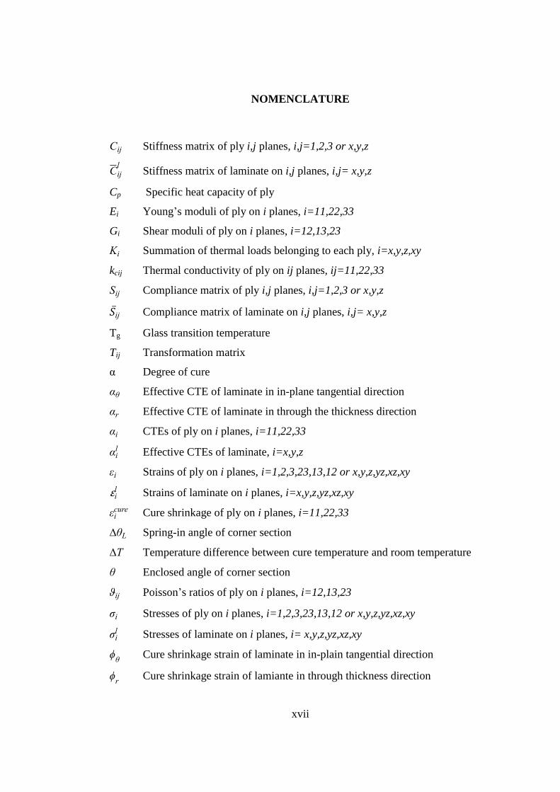
NOMENCLATURE
i Stiffness matrix of ply i,j planes, i,j=1,2,3 or x,y,z
i
Stiffness matrix of laminate on i,j planes, i,j= x,y,z
Cp Specific heat capacity of ply
Ei Young’s moduli of ply on i planes, i=11,22,33
Gi Shear moduli of ply on i planes, i=12,13,23
i Summation of thermal loads belonging to each ply, i=x,y,z,xy
kcij Thermal conductivity of ply on ij planes, ij=11,22,33
i Compliance matrix of ply i,j planes, i,j=1,2,3 or x,y,z
i Compliance matrix of laminate on i,j planes, i,j= x,y,z
Tg Glass transition temperature
Tij Transformation matrix
α Degree of cure
Effective CTE of laminate in in-plane tangential direction
Effective CTE of laminate in through the thickness direction
i CTEs of ply on i planes, i=11,22,33
i Effective CTEs of laminate, i=x,y,z
i Strains of ply on i planes, i=1,2,3,23,13,12 or x,y,z,yz,xz,xy
i Strains of laminate on i planes, i=x,y,z,yz,xz,xy
ic Cure shrinkage of ply on i planes, i=11,22,33
Spring-in angle of corner section
T Temperature difference between cure temperature and room temperature
Enclosed angle of corner section
i Poisson’s ratios of ply on i planes, i=12,13,23
i Stresses of ply on i planes, i=1,2,3,23,13,12 or x,y,z,yz,xz,xy
i Stresses of laminate on i planes, i= x,y,z,yz,xz,xy
Cure shrinkage strain of laminate in in-plain tangential direction
Cure shrinkage strain of lamiante in through thickness direction

xviii
LIST OF ABBREVIATIONS
CAD Computer Aided Design
CLT Classical Lamination Theory
CMC Ceramic Matrix Composite
CNC Computer Numerical Control
CTE Coefficient of Thermal Expansion
FEA Finite Element Analysis
FEM Finite Element Method
FRPC Fiber-reinforced Plastic Composite
MMC Metal Matrix Composite
PMC Polymer Matrix Composite
RTM Resin Transfer Molding
UD Unidirectional
USDFLD User Defined Field
3-D Three dimensional
2-D Two dimensional
1
CHAPTER 1
INTRODUCTION
1.1 COMPOSITE MATERIALS
A composite material, or sometimes called as a composite, is a combination of at
least two materials which have different physical and chemical properties. The
concept of composite is first encountered in the nature although today, composite
materials are commonly considered as engineered materials. For example, natural
wood is a composite material. It consists of cellulose fibers embedded in
polysaccharide lignin. Here, cellulose fibers are responsible from providing good
strength and stiffness properties while the polysaccharide lignin as the resin matrix
ensures the integrity of the wood [1].
Composite materials with their changeable mechanical properties allow designers to
overcome difficult engineering problems by making tougher and lighter designs
possible. Moreover, manufacturing complex shaped parts with the use of
composites is easier than with the use of conventional materials such as metals. The
composite materials have many other advantageous properties which are good
dimensional stability, corrosion resistance, slowness of damage propagation, good
fatigue strength, and aging resistance [2]. Therefore, the use of composite materials
takes place in various industries such as automotive industry, building and civil
engineering industry, aeronautics, space, armaments, shipbuilding, electricity and
electronics, sports and leisure industries, and many other industries like packaging,
art, and decoration [3].
Modern composite materials can be classified in four categories based on their
matrices: polymer matrix composite (PMC), metal matrix composite (MMC),
ceramic matrix composite (CMC), and carbon matrix composite. Much lower
manufacturing temperatures are required for PMC when compared to MMC and
2
CMC. Also, there has been an increasing demand over the last 30 years in the usage
of PMC, particularly for fiber-reinforced plastic composites (FRPC) [4]. PMC
contains thermoset or thermoplastic resins which are reinforced with glass, carbon,
aramid, or boron fibers. MMC includes metals or alloys reinforced with boron,
carbon, or ceramic fibers. CMC, on the other hand, is composed of ceramic matrix
and ceramic fibers. Carbon matrix composites employ graphite yarn or fabric in
carbon or graphite matrix [9].
In this study, the focus will be on PMC which has two different types in terms of its
polymer matrices such as thermoset composites and thermoplastic composites. As
will be explained in the following chapters, these composites are reinforced with
fiber structures and manufactured by different processes.
1.1.1 Thermoset Composites
A set of manufacturing methods are available for thermoset composites such as
hand lay-up, liquid composite moulding (e.g. resin transfer molding or RTM
process), and autoclave-forming [5].
Thermoset resins become hardened (solid-like) material when they are cured by
applying heat for a specific time interval. However, when a thermoset resin is
heated or cured, the process is irreversible which means the resin can not be
remolded after the initial heat-forming or curing process. Heating a thermoset resin
forms three-dimensional (3-D) network structure between the molecules of resin as
chemical reactions (chemical crosslinking or sometimes called as polymerization
reactions) take place during curing process. Therefore, once cured, thermoset resins
still sustain their strength and shape at high temperatures and they will not become
liquid when they are reheated. But above a certain temperature, a dramatic fall in
the mechanical properties of thermoset resin is observed. This temperature is called
as glass transition temperature (T ). T differs for each thermoset resin depending
upon the specific cure-cycle parameters such as time, temperature, and pressure [4].
3
As the thermoset resins can stay in liquid state at low temperatures before the cure
process, embedding continuous fiber reinforcements into the resin matrix can be
performed relatively easily. For that reason, thermoset composites are widely
available with continuous fiber reinforcements. Epoxy, vinyl ester, furan, cyanate
ester, bismaleimide, phenolic resin, and unsaturated polyester can be given as
examples to the thermoset resins that are used in the fiber reinforced composites [4].
1.1.2 Thermoplastic Composites
Thermoplastic composites can be processed by different manufacturing methods.
For instance, autoclave-forming, diaphragm forming, and compression-forming are
the most commonly used methods [5].
Thermoplastic resins, on the other hand, become softened when they are heated and
become hardened or solidified when they are cooled down. It is possible to heat up
and cool down a thermoplastic resin system as many times as needed without
causing a chemical change in the resin’s molecular structure. This means the
manufacturing process of thermoplastic resin composites is reversible [6, 22].
PET, polyproplyene, polycarbonate, PBT, vinyl, polyethylene, PVC, PEI, and nylon
can be given as examples to commonly used thermoplastic resins. Thermoplastic
composites with short-chopped fiber reinforcements have been widely employed in
thermoplastic composite industry and this type of thermoplastic composites
generally contains glass or carbon fiber as the reinforcement. However, for the last
decade, it has been possible to see long fiber thermoplastic composite applications
in composite industries, especially in automotive industry. These materials have
advantages in terms of material properties and manufacturing processes such as
adjustable and reproducible fiber length distribution, single heat history, high
productivity, and short cycle times [7, 8].
4
1.1.3 Fiber Reinforcements
In FRPC, fibers can be in different structural forms such as small particles, whiskers
(discontinuous fibers) or continuous fibers (filaments). Glass, carbon, and aramid
are the most commonly used fiber types in engineering composites and there are
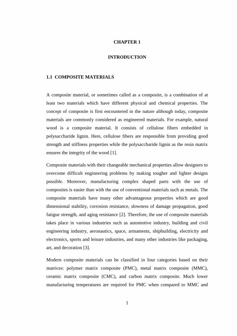
some other types of fibers available like boron and ceramic [9]. Fiber arrangement
in a laminate can be two dimensional (2-D) or three dimensional (3-D). For the 2-D
fiber arrangement, there is no fiber aligned in through thickness direction (Figure
1). However, this leads to poor mechanical properties in terms of stiffness and
strength in this direction. As the through-thickness direction of the laminate is
dominated with resin which has weaker mechanical properties when compared to
the in-plane fiber dominated properties [10]. (Figure 2)
Figure 1: Schematic of 2-D fiber arrangement [10]
5
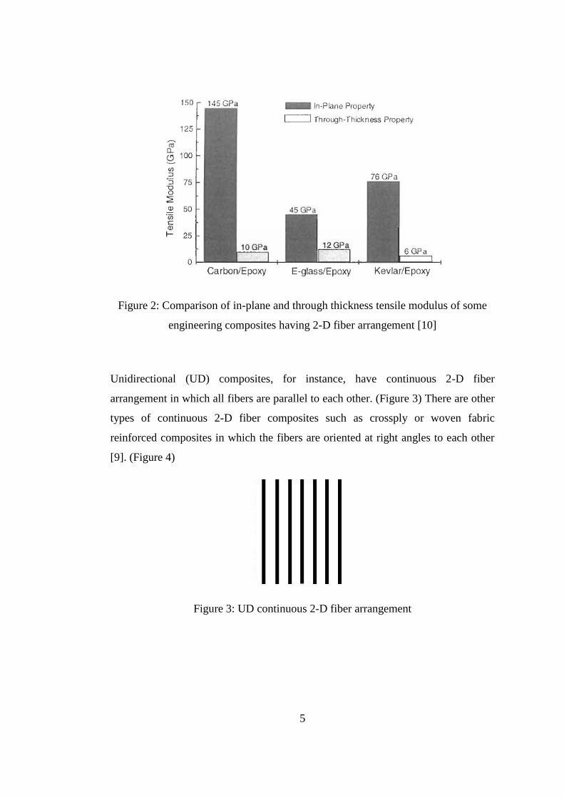
Figure 2: Comparison of in-plane and through thickness tensile modulus of some
engineering composites having 2-D fiber arrangement [10]
Unidirectional (UD) composites, for instance, have continuous 2-D fiber
arrangement in which all fibers are parallel to each other. (Figure 3) There are other
types of continuous 2-D fiber composites such as crossply or woven fabric
reinforced composites in which the fibers are oriented at right angles to each other
[9]. (Figure 4)
Figure 3: UD continuous 2-D fiber arrangement
6
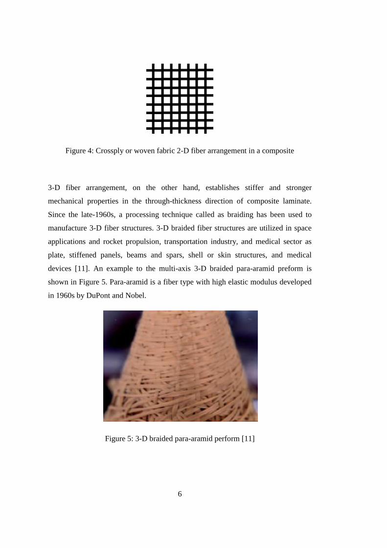
Figure 4: Crossply or woven fabric 2-D fiber arrangement in a composite
3-D fiber arrangement, on the other hand, establishes stiffer and stronger
mechanical properties in the through-thickness direction of composite laminate.
Since the late-1960s, a processing technique called as braiding has been used to
manufacture 3-D fiber structures. 3-D braided fiber structures are utilized in space
applications and rocket propulsion, transportation industry, and medical sector as
plate, stiffened panels, beams and spars, shell or skin structures, and medical
devices [11]. An example to the multi-axis 3-D braided para-aramid preform is
shown in Figure 5. Para-aramid is a fiber type with high elastic modulus developed
in 1960s by DuPont and Nobel.
Figure 5: 3-D braided para-aramid perform [11]
7
1.1.4 Manufacturing Processes
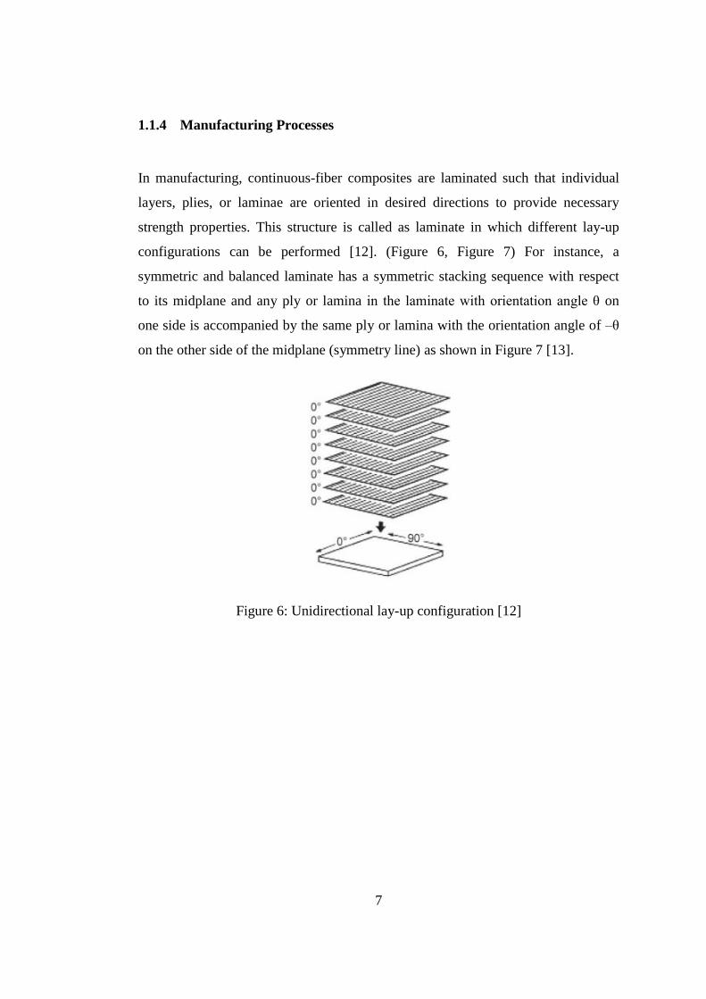
In manufacturing, continuous-fiber composites are laminated such that individual
layers, plies, or laminae are oriented in desired directions to provide necessary
strength properties. This structure is called as laminate in which different lay-up
configurations can be performed [12]. (Figure 6, Figure 7) For instance, a
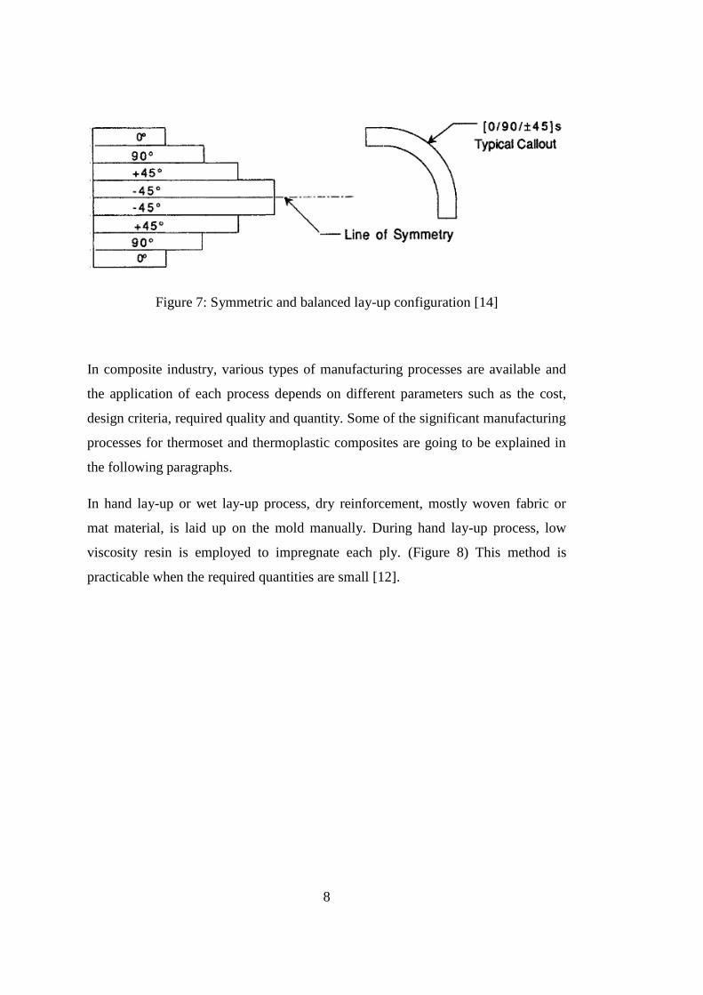
symmetric and balanced laminate has a symmetric stacking sequence with respect
to its midplane and any ply or lamina in the laminate with orientation angle θ on
one side is accompanied by the same ply or lamina with the orientation angle of –θ
on the other side of the midplane (symmetry line) as shown in Figure 7 [13].
Figure 6: Unidirectional lay-up configuration [12]
8
Figure 7: Symmetric and balanced lay-up configuration [14]
In composite industry, various types of manufacturing processes are available and
the application of each process depends on different parameters such as the cost,
design criteria, required quality and quantity. Some of the significant manufacturing
processes for thermoset and thermoplastic composites are going to be explained in
the following paragraphs.
In hand lay-up or wet lay-up process, dry reinforcement, mostly woven fabric or
mat material, is laid up on the mold manually. During hand lay-up process, low
viscosity resin is employed to impregnate each ply. (Figure 8) This method is
practicable when the required quantities are small [12].
9
Figure 8: Hand lay-up process [12]
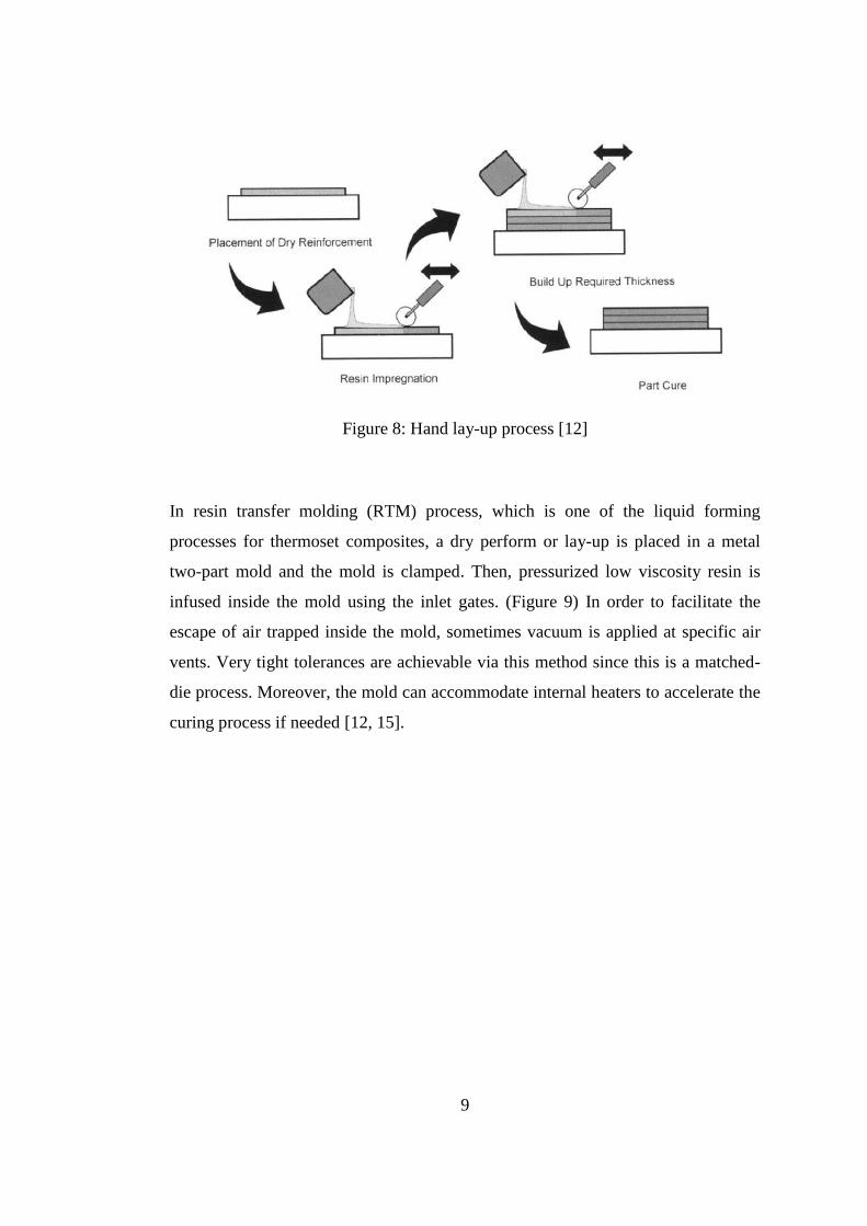
In resin transfer molding (RTM) process, which is one of the liquid forming
processes for thermoset composites, a dry perform or lay-up is placed in a metal
two-part mold and the mold is clamped. Then, pressurized low viscosity resin is
infused inside the mold using the inlet gates. (Figure 9) In order to facilitate the
escape of air trapped inside the mold, sometimes vacuum is applied at specific air
vents. Very tight tolerances are achievable via this method since this is a matched-
die process. Moreover, the mold can accommodate internal heaters to accelerate the
curing process if needed [12, 15].
10
Figure 9: RTM process [12]
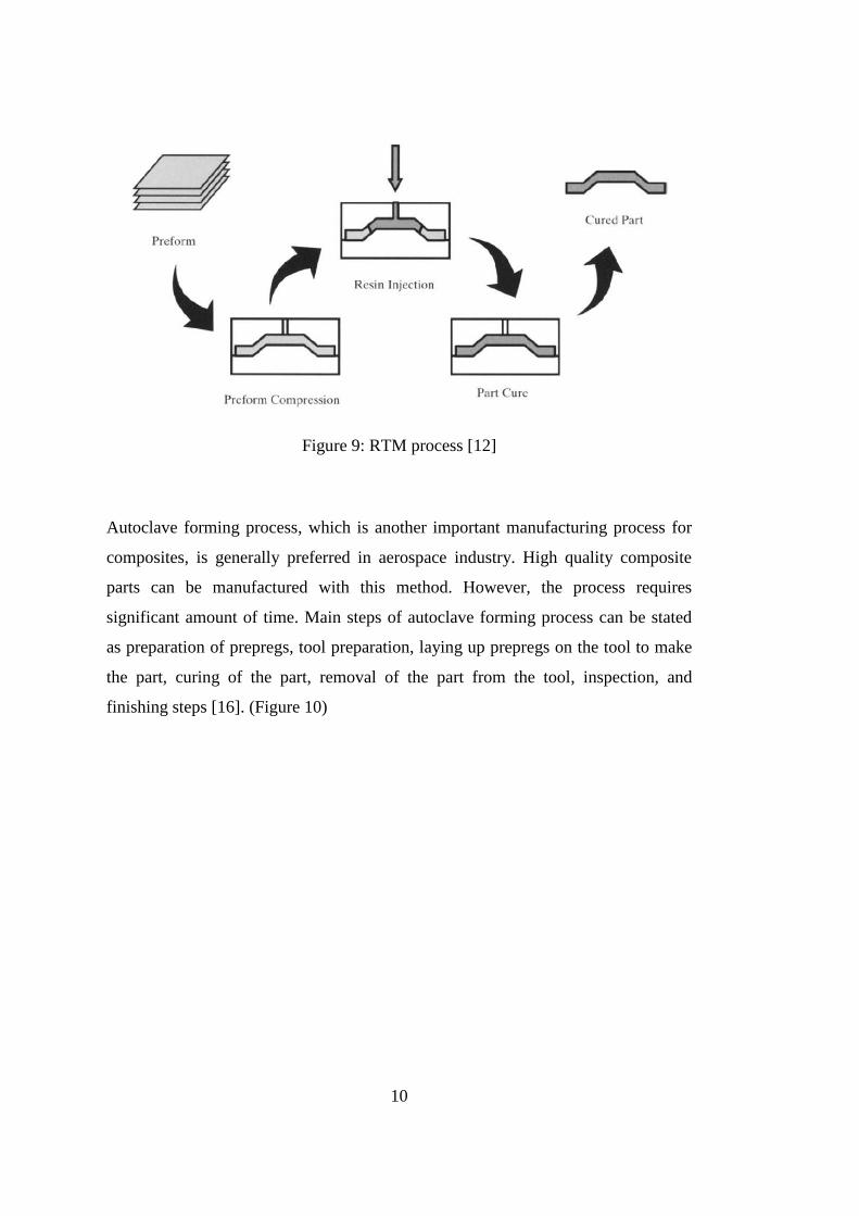
Autoclave forming process, which is another important manufacturing process for
composites, is generally preferred in aerospace industry. High quality composite
parts can be manufactured with this method. However, the process requires
significant amount of time. Main steps of autoclave forming process can be stated
as preparation of prepregs, tool preparation, laying up prepregs on the tool to make
the part, curing of the part, removal of the part from the tool, inspection, and
finishing steps [16]. (Figure 10)
11
Figure 10: Autoclave forming process [16]
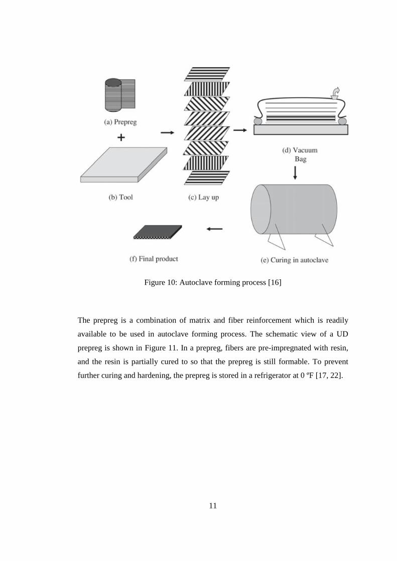
The prepreg is a combination of matrix and fiber reinforcement which is readily
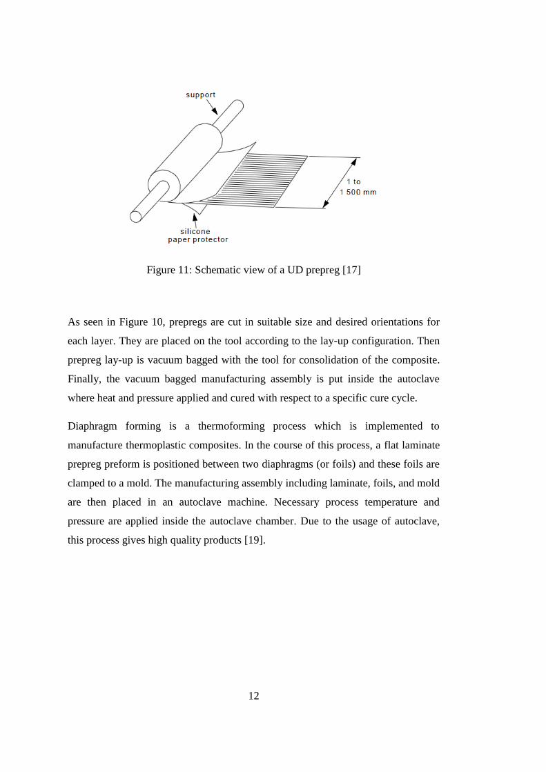
available to be used in autoclave forming process. The schematic view of a UD
prepreg is shown in Figure 11. In a prepreg, fibers are pre-impregnated with resin,
and the resin is partially cured to so that the prepreg is still formable. To prevent
further curing and hardening, the prepreg is stored in a refrigerator at 0 ºF [17, 22].
12
Figure 11: Schematic view of a UD prepreg [17]
As seen in Figure 10, prepregs are cut in suitable size and desired orientations for
each layer. They are placed on the tool according to the lay-up configuration. Then
prepreg lay-up is vacuum bagged with the tool for consolidation of the composite.
Finally, the vacuum bagged manufacturing assembly is put inside the autoclave
where heat and pressure applied and cured with respect to a specific cure cycle.
Diaphragm forming is a thermoforming process which is implemented to
manufacture thermoplastic composites. In the course of this process, a flat laminate
prepreg preform is positioned between two diaphragms (or foils) and these foils are
clamped to a mold. The manufacturing assembly including laminate, foils, and mold
are then placed in an autoclave machine. Necessary process temperature and
pressure are applied inside the autoclave chamber. Due to the usage of autoclave,
this process gives high quality products [19].
13
1.2 MANUFACTURING INDUCED SHAPE DISTORTION PROBLEMS IN
THERMOSET COMPOSITES VIA AUTOCLAVE FORMING PROCESS
1.2.1 Vacuum Bagging and Cure Cycle
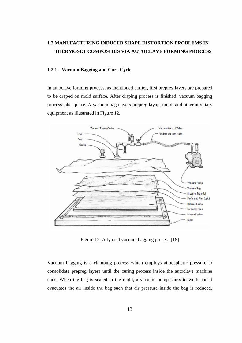
In autoclave forming process, as mentioned earlier, first prepreg layers are prepared
to be draped on mold surface. After draping process is finished, vacuum bagging
process takes place. A vacuum bag covers prepreg layup, mold, and other auxiliary
equipment as illustrated in Figure 12.
Figure 12: A typical vacuum bagging process [18]
Vacuum bagging is a clamping process which employs atmospheric pressure to
consolidate prepreg layers until the curing process inside the autoclave machine
ends. When the bag is sealed to the mold, a vacuum pump starts to work and it
evacuates the air inside the bag such that air pressure inside the bag is reduced.

14
Then atmospheric pressure puts equal force on everywhere of the vacuum bag
surface. The pressure gradient between inside and outside of the vacuum bag drives
the amount of clamping force [18].
Breather material shown in Figure 12 is a perforated film which endures high
temperatures in autoclave chamber. It allows the escape of vapor of gases formed
during curing process. Release fabric, on the other hand, is a smooth fabric which
does not stick to the laminate. It provides a good surface quality for the laminate.
Sometimes, release agents are applied on the mold surface to prevent laminates
from bonding to the mold surface [16, 18].
Mastic sealant or sealant tape is used during vacuum bagging process for sealing the
interface between mold and bagging film. The sealant should adhere to mold
surface properly in order to provide an airtight seal [20].
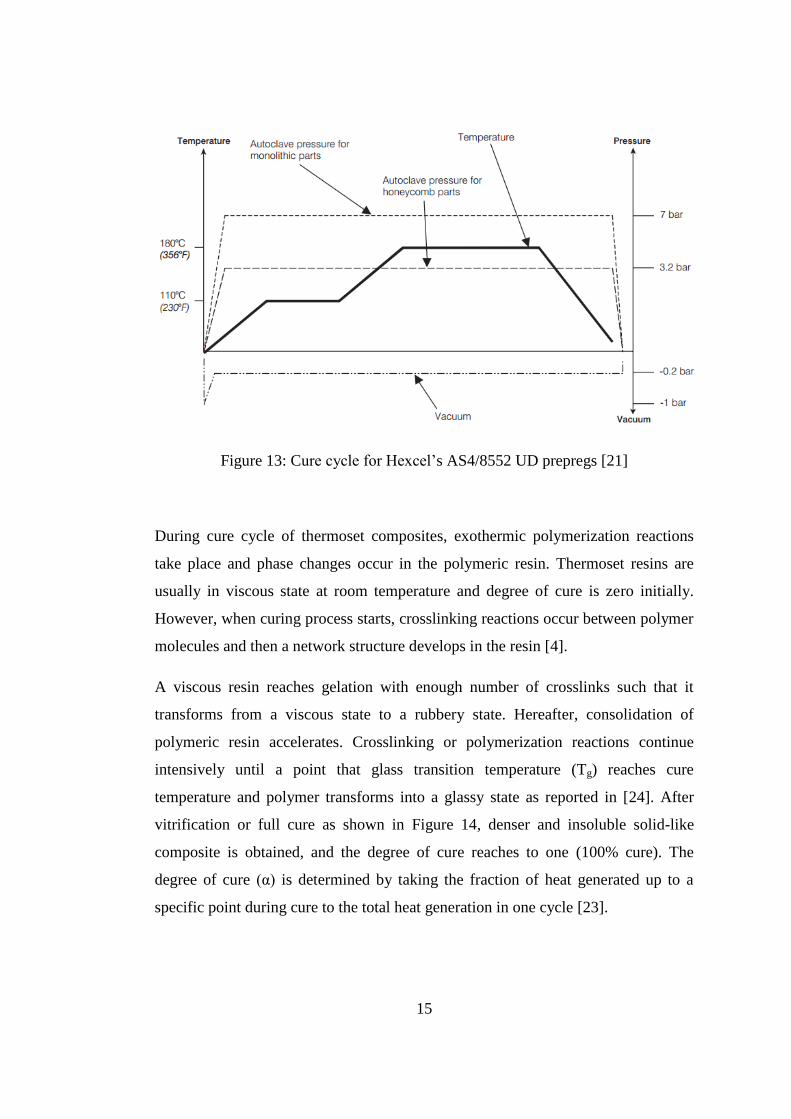
After vacuum bagging process is completed, manufacturing assembly is placed in to
autoclave chamber. Inside the autoclave, in order to accomplish curing process, the
manufacturing assembly is subjected to temperature and pressure cycles with
respect to a time cycle. The combination of these cycles is called as cure cycle and
as an example, cure cycle for a specific prepreg is shown in Figure 13 [16].
15
Figure 13: Cure cycle for Hexcel’s AS4/8552 UD prepregs [21]
During cure cycle of thermoset composites, exothermic polymerization reactions
take place and phase changes occur in the polymeric resin. Thermoset resins are
usually in viscous state at room temperature and degree of cure is zero initially.
However, when curing process starts, crosslinking reactions occur between polymer
molecules and then a network structure develops in the resin [4].
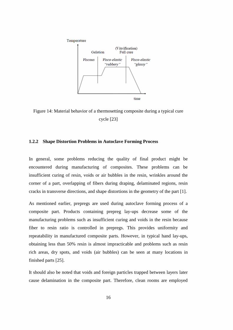
A viscous resin reaches gelation with enough number of crosslinks such that it
transforms from a viscous state to a rubbery state. Hereafter, consolidation of
polymeric resin accelerates. Crosslinking or polymerization reactions continue
intensively until a point that glass transition temperature (Tg) reaches cure
temperature and polymer transforms into a glassy state as reported in [24]. After
vitrification or full cure as shown in Figure 14, denser and insoluble solid-like
composite is obtained, and the degree of cure reaches to one (100% cure). The
degree of cure (α) is determined by taking the fraction of heat generated up to a
specific point during cure to the total heat generation in one cycle [23].
16
Figure 14: Material behavior of a thermosetting composite during a typical cure
cycle [23]
1.2.2 Shape Distortion Problems in Autoclave Forming Process
In general, some problems reducing the quality of final product might be
encountered during manufacturing of composites. These problems can be
insufficient curing of resin, voids or air bubbles in the resin, wrinkles around the
corner of a part, overlapping of fibers during draping, delaminated regions, resin
cracks in transverse directions, and shape distortions in the geometry of the part [1].
As mentioned earlier, prepregs are used during autoclave forming process of a
composite part. Products containing prepreg lay-ups decrease some of the
manufacturing problems such as insufficient curing and voids in the resin because
fiber to resin ratio is controlled in prepregs. This provides uniformity and
repeatability in manufactured composite parts. However, in typical hand lay-ups,
obtaining less than 50% resin is almost impracticable and problems such as resin
rich areas, dry spots, and voids (air bubbles) can be seen at many locations in
finished parts [25].
It should also be noted that voids and foreign particles trapped between layers later
cause delamination in the composite part. Therefore, clean rooms are employed
17
during draping of prepreg layers in order to prevent foreign particles from sticking
to layer surfaces and vacuum bag is utilized in autoclave forming process to
decrease the amount of voids present in the resin. It is particularly important to
apply vacuum bagging to reduce voids since interlaminar shear strength reduces by
7% for each 1% void present in the resin [28].
Resin cracks are considered to initiate from manufacturing defects such as resin
voids, densely grouped fiber arrangement, and fiber-resin de-bonding. These cracks
can grow within planes normal to the ply mid-plane and finally result in failure
[29].
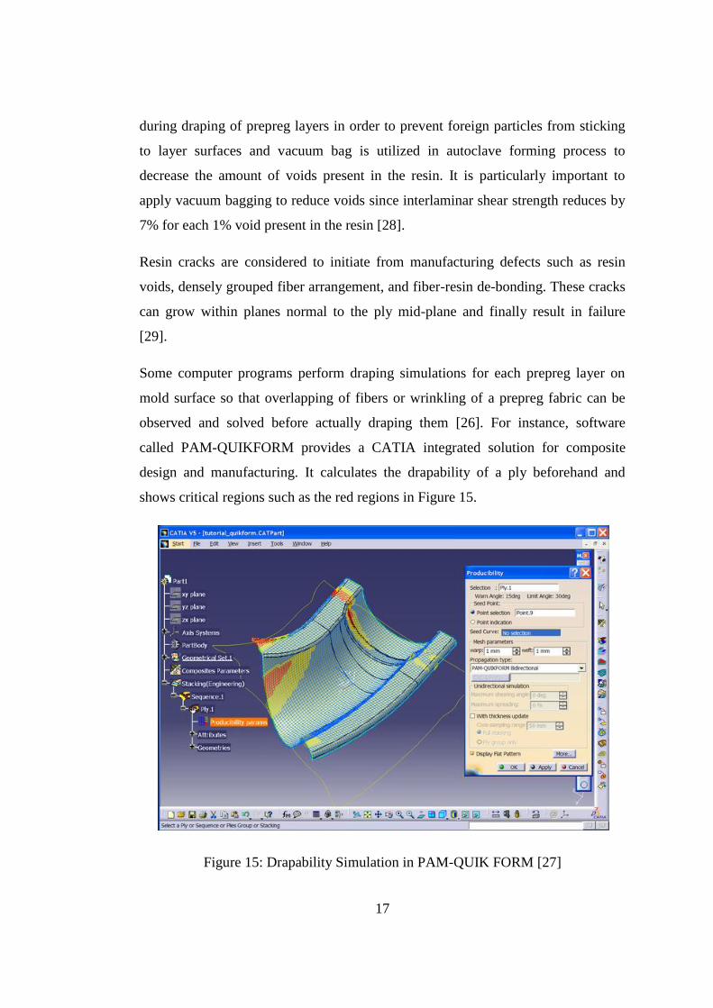
Some computer programs perform draping simulations for each prepreg layer on
mold surface so that overlapping of fibers or wrinkling of a prepreg fabric can be
observed and solved before actually draping them [26]. For instance, software
called PAM-QUIKFORM provides a CATIA integrated solution for composite
design and manufacturing. It calculates the drapability of a ply beforehand and
shows critical regions such as the red regions in Figure 15.
Figure 15: Drapability Simulation in PAM-QUIK FORM [27]
18
Manufacturing problems mentioned up to this point can be controlled and
eliminated in the course of an autoclave forming process. However, shape
distortions which occur due to unavoidable residual stress formations during cure
are not easy to overcome [23]. Because of shape distortions, assembling of
composite parts becomes difficult and this leads to an increase in manufacturing
costs. In the following sections, shape distortion types and mechanisms causing
residual stresses and shape distortions are going to be explained in detail.
1.2.2.1. Shape Distortion Types
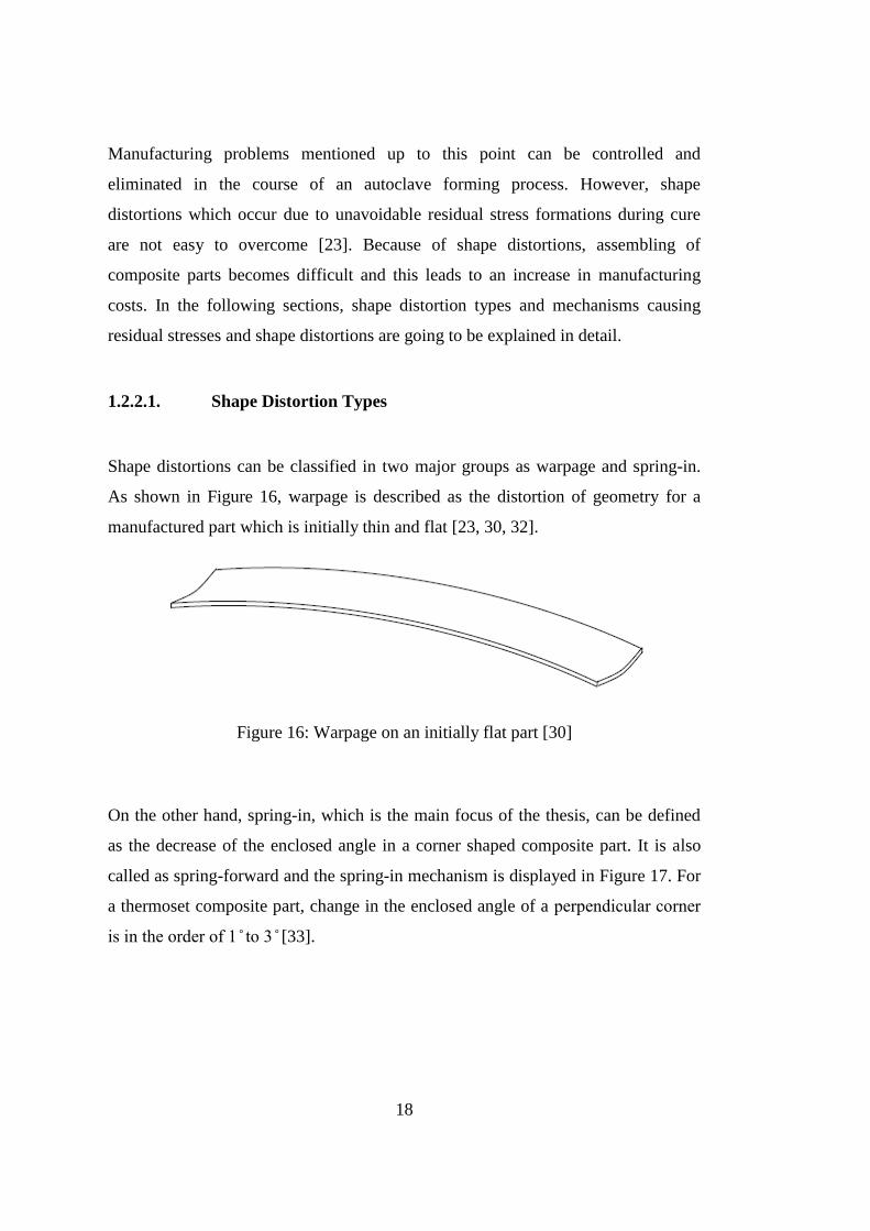
Shape distortions can be classified in two major groups as warpage and spring-in.
As shown in Figure 16, warpage is described as the distortion of geometry for a
manufactured part which is initially thin and flat [23, 30, 32].
Figure 16: Warpage on an initially flat part [30]
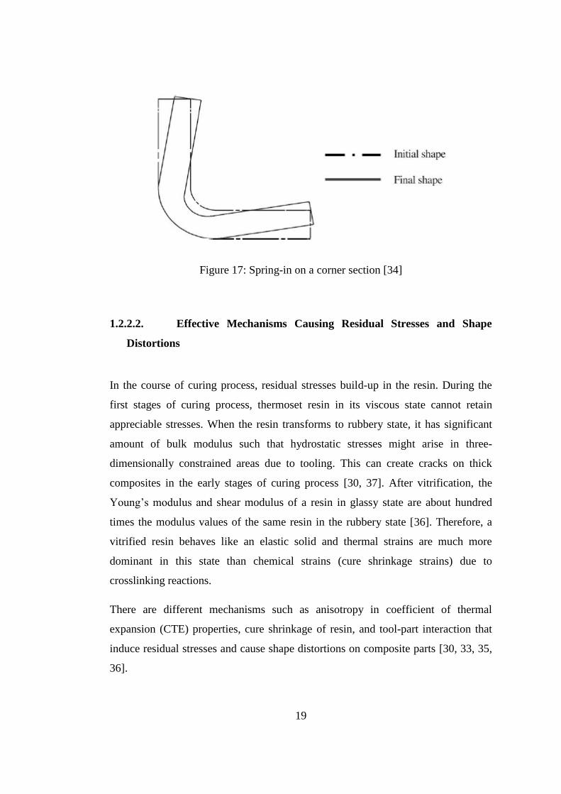
On the other hand, spring-in, which is the main focus of the thesis, can be defined
as the decrease of the enclosed angle in a corner shaped composite part. It is also
called as spring-forward and the spring-in mechanism is displayed in Figure 17. For
a thermoset composite part, change in the enclosed angle of a perpendicular corner
is in the order of 1 to 3 [33].
19
Figure 17: Spring-in on a corner section [34]
1.2.2.2. Effective Mechanisms Causing Residual Stresses and Shape
Distortions
In the course of curing process, residual stresses build-up in the resin. During the
first stages of curing process, thermoset resin in its viscous state cannot retain
appreciable stresses. When the resin transforms to rubbery state, it has significant
amount of bulk modulus such that hydrostatic stresses might arise in three-
dimensionally constrained areas due to tooling. This can create cracks on thick
composites in the early stages of curing process [30, 37]. After vitrification, the
Young’s modulus and shear modulus of a resin in glassy state are about hundred
times the modulus values of the same resin in the rubbery state [36]. Therefore, a
vitrified resin behaves like an elastic solid and thermal strains are much more
dominant in this state than chemical strains (cure shrinkage strains) due to
crosslinking reactions.
There are different mechanisms such as anisotropy in coefficient of thermal
expansion (CTE) properties, cure shrinkage of resin, and tool-part interaction that
induce residual stresses and cause shape distortions on composite parts [30, 33, 35,
36].
20
Anisotropy in CTEs
There are three mechanisms causing residual stresses because of anisotropic CTE
properties. These mechanisms are due to fiber and matrix level (micromechanical
level), ply-level, and laminate-level differential thermal expansion properties
respectively [30].
In the first mechanism, it is stated that CTE of polymer-matrix is generally higher
than the CTE of fiber. In addition to this, fibers generally have orthotropic thermal
expansion coefficients. This means CTE’s of a fiber are unique and independent in
three mutually perpendicular directions. These factors result in residual stresses at
the micromechanical level as the part is cooled-down from the cure temperature to
the room temperature. The residual stresses developed at this level do not contribute
much to the shape distortions, however; they might cause the progress of matrix
cracking and have a negative effect on the mechanical properties of the composites
[30, 37].
Unidirectional plies have much larger CTE in the transverse directions than in the
fiber direction because the fiber direction is dominated by fibers whereas the
transverse directions are dominated by resin. Furthermore, the mechanical stiffness
properties of unidirectional composites are much weaker in transverse direction
when compared to the fiber direction [36]. Therefore, in the second mechanism,
when the temperature of a ply is increased, transverse expansion is more than
expansion observed in the fiber direction and as a result warpage in the initially flat
ply is encountered [30].
The third mechanism is similar to the second mechanism but this time it is in the
laminate-level. Laminates, having higher transverse CTE’s compared to fiber
dominated longitudinal CTE, tend to distort with the application of temperature
gradient [30]. However, transverse expansion of a laminate is greatly dependent up
on the lay-up configuration. If an initially flat laminate is symmetric and balanced,
then all stretch-bending couplings are eliminated such that transverse expansions of
21
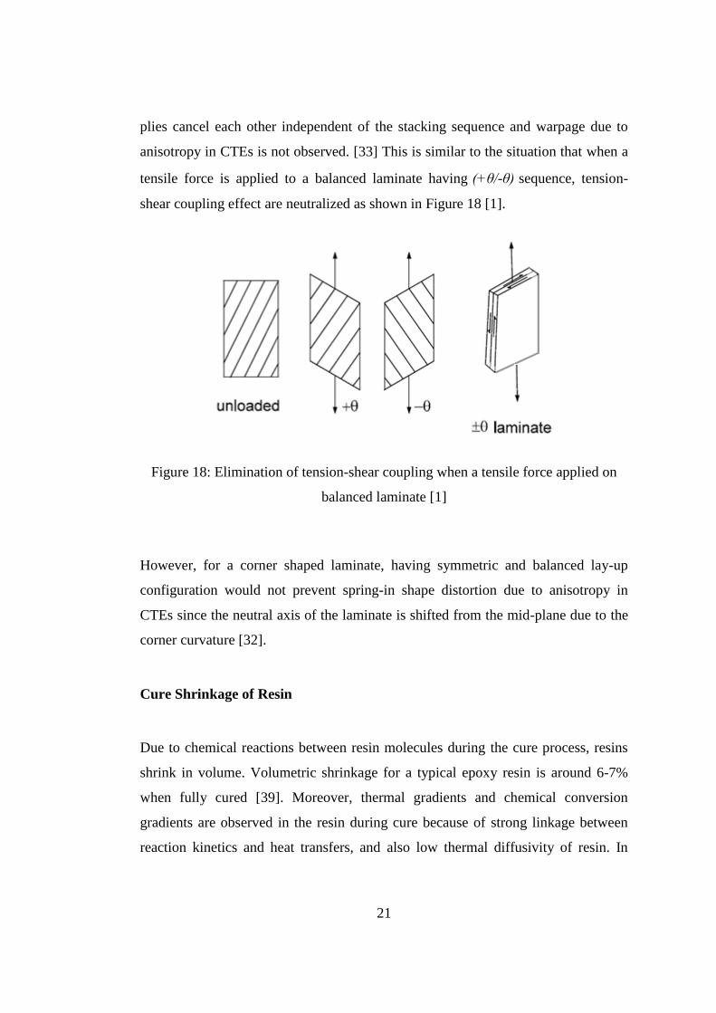
plies cancel each other independent of the stacking sequence and warpage due to
anisotropy in CTEs is not observed. [33] This is similar to the situation that when a
tensile force is applied to a balanced laminate having - sequence, tension-
shear coupling effect are neutralized as shown in Figure 18 [1].
Figure 18: Elimination of tension-shear coupling when a tensile force applied on
balanced laminate [1]
However, for a corner shaped laminate, having symmetric and balanced lay-up
configuration would not prevent spring-in shape distortion due to anisotropy in
CTEs since the neutral axis of the laminate is shifted from the mid-plane due to the
corner curvature [32].
Cure Shrinkage of Resin
Due to chemical reactions between resin molecules during the cure process, resins
shrink in volume. Volumetric shrinkage for a typical epoxy resin is around 6-7%
when fully cured [39]. Moreover, thermal gradients and chemical conversion
gradients are observed in the resin during cure because of strong linkage between
reaction kinetics and heat transfers, and also low thermal diffusivity of resin. In
22
thick laminates, thermal gradients through thickness direction have significant
effect on curing process and they can change the cure shrinkage trend [40]. The
difference in degree of cure between the surface and core of a neat resin reaches to
15% of the total degree of cure [39]. This causes residual stresses and cure gradients
in the resin and leads to variation in mechanical properties. In addition to this,
chemical shrinkage causes shape distortions in curved or cylindrical laminates due
to the different chemical shrinkage buildup between in-plane and transverse
directions [41].
Cure shrinkage can be minimized through the use of different cure cycles. For that
purpose, time and temperature parameters of cure cycle are modified [42].
However, modifying cure cycle parameters to reduce residual stresses is not always
feasible since there might be an increase in the time of curing process or undesired
mechanical properties can be obtained at the end.
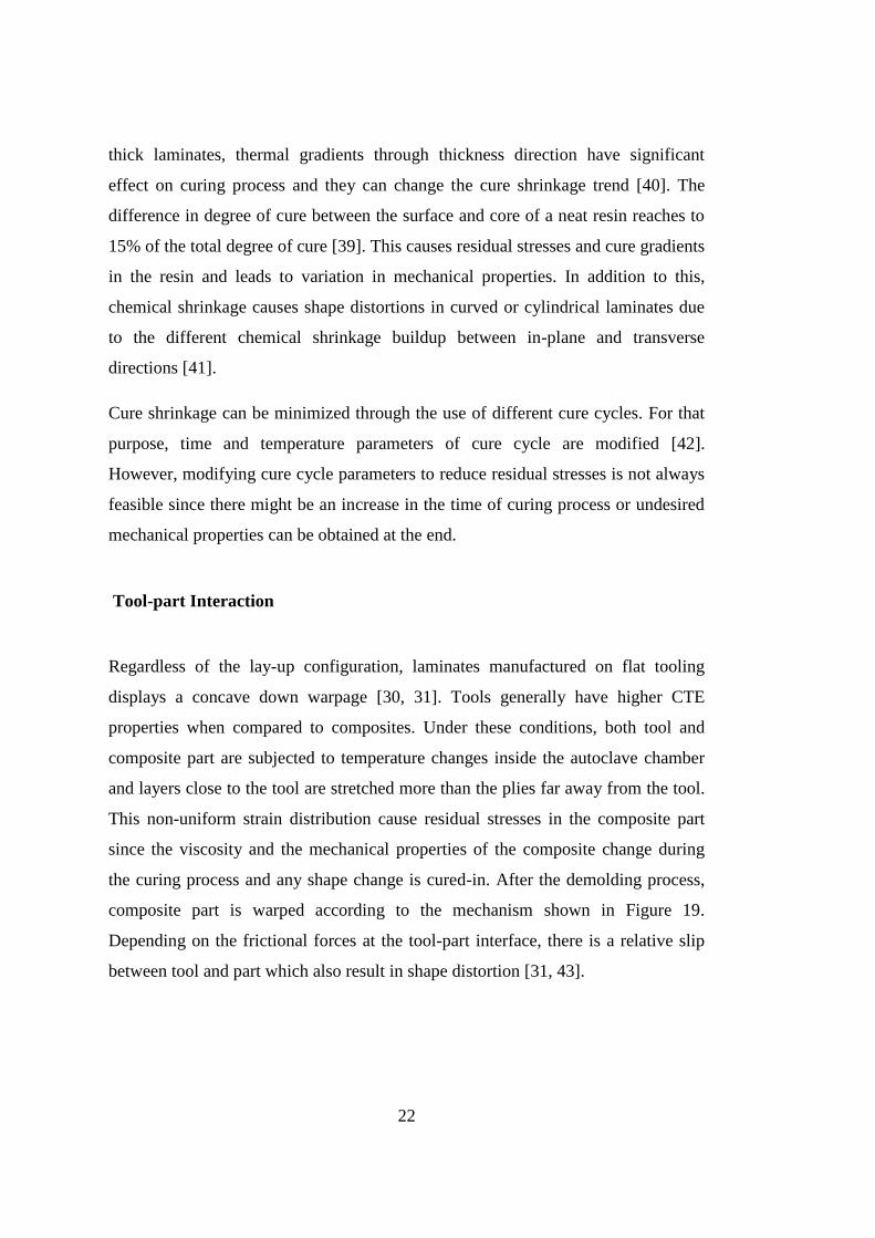
Tool-part Interaction
Regardless of the lay-up configuration, laminates manufactured on flat tooling
displays a concave down warpage [30, 31]. Tools generally have higher CTE
properties when compared to composites. Under these conditions, both tool and
composite part are subjected to temperature changes inside the autoclave chamber
and layers close to the tool are stretched more than the plies far away from the tool.
This non-uniform strain distribution cause residual stresses in the composite part
since the viscosity and the mechanical properties of the composite change during
the curing process and any shape change is cured-in. After the demolding process,
composite part is warped according to the mechanism shown in Figure 19.
Depending on the frictional forces at the tool-part interface, there is a relative slip
between tool and part which also result in shape distortion [31, 43].
23
Figure 19: Warpage Mechanism: a) Tool expansion due to heating of tool up to cure
temperature b) Inter-ply slippage due to stress gradients in the through thickness
direction c) Initially flat part is curved after demolding [31]
1.3 OBJECTIVE OF THE THESIS
The objective of this thesis is to develop a 3-D numerical analysis model that
predicts the spring-in problem in corner shaped composite parts manufactured via
autoclave forming process. It is considered that with such a predictive analysis
method, tool geometry can be modified beforehand such that the cured part comes
out of the mold without any appreciable shape distortion. For this purpose, an
efficient and reliable numerical analysis model which considers anisotropic material
behavior, cure shrinkage of resin, and tool-part interaction is developed.
1.4 THESIS OUTLINE
This thesis consists of five main chapters. In the first three chapters, spring-in
problem on corner shaped composite parts which are made of AS4/8552 composite
system is investigated by different methods. AS4/8552 is a UD prepreg which
24
consists of carbon fibers and epoxy resin. Then, in the last two chapters, results are
presented and discussed, and conclusions are made respectively.
2-D analytical solution for spring-in problem available in the literature is presented
in Chapter 2. The analytical solution finds and uses 3-D effective CTEs of a
symmetric and balanced laminate. Furthermore, the effect of cure shrinkage is also
taken into account here and for that purpose; effective cure shrinkage strains of a
symmetric and balanced laminate are also found. Then strains due to anisotropy in
CTEs and cure shrinkage are utilized in a simple geometric formula to find spring-
in angle of a corner shaped composite part.
In Chapter 3, spring-in behavior of U-shaped composite parts is examined by
manufacturing composite specimens using autoclave forming process. For that
purpose, details of spring-in angle measurement using an optical scanning device
are described. Also, in this chapter it is explained how the surface temperature field
of a specific manufacturing assembly inside the autoclave chamber is monitored
during the curing process.
A 3-D ABAQUS model simulating the spring-in of U-shaped composite parts is
developed in Chapter 4. The numerical model considers changing rubbery and
glassy state composite properties and takes spring-in mechanisms such as
anisotropy in material properties, cure shrinkage of resin and tool-part interaction
into account. In addition to these, the effects of cure shrinkage and tool-part
interaction mechanisms on spring-in problem are separately identified numerically.
Results of analytical, experimental and numerical spring-in values are given and
discussed in Chapter 5. Comments are made on the effects of cure shrinkage and
tool-part interaction mechanisms on spring-in problem. In addition to these, the
effect of coefficient of friction between tool and part is discussed.
In Chapter 6, conclusions are made and recommendations for further research are
provided.
25
CHAPTER 2
ANALYTICAL DETERMINATION OF SPRING-IN
In this chapter, a 2-D theoretical computation method available in the literature for
spring-in on corner sections is explained and a solution is obtained with this
method. The method includes both the anisotropy in CTE and the cure shrinkage
effects, but excludes tool-part interaction. The aim is to compare the results
obtained using the analytical method with experimental measurements and the FEM
solution.
2.1 GEOMETRIC DEFINITION OF SPRING-IN
Spring-in is already discussed in Chapter 1 and it can be defined as the decrease in
the enclosed angle of a corner section which has anisotropic material properties.
There have been many studies conducted to determine spring-in angle theoretically
over the past years. [33, 34, 41, 44, 45, 46] In this chapter, a theoretical model
solving the spring-in angle of a corner section on a laminate is introduced.
Theoretical model utilizes 2-D Radford model [46] to take both cure shrinkage and
anisotropy of CTE into account during cooling down from cure temperature to room
temperature with the help of studies available in the literature [33, 44].
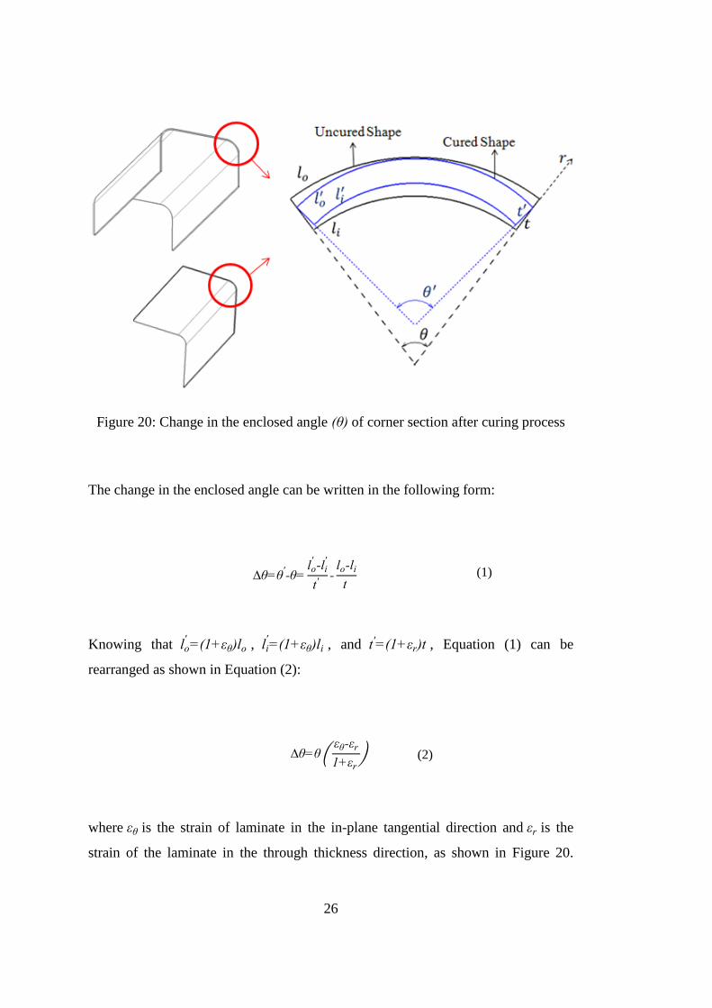
Corner section of a U-shaped or L-shaped composite part in cured and uncured
states is displayed in Figure 20 where o, i, and represent the enclosed angle,
outer length, inner length and thickness of the corner section in uncured state,
respectively.
26
Figure 20: Change in the enclosed angle of corner section after curing process
The change in the enclosed angle can be written in the following form:
o i
o i
(1)
Knowing that o o , i
i , and , Equation (1) can be
rearranged as shown in Equation (2):
(2)
where is the strain of laminate in the in-plane tangential direction and is the
strain of the laminate in the through thickness direction, as shown in Figure 20.
27
Using Equation (2), the sources of in-plane and through thickness strains such as
anisotropy in CTE ( T ) and cure shrinkage ( ) are included and expanded in
Equation (3).
T T
T
(3)
where, , , , , and T denote CTE in in-plane tangential direction, CTE in
through the thickness direction, cure shrinkage strain in in-plane tangential
direction, cure shrinkage strain in through the thickness direction, and temperature
difference between the cure temperature and the room temperature, respectively.
Although, the formula given in Equation (3) models a 2-D spring-in problem, the
need for calculating effective CTEs ( and ) of the laminate in through the
thickness and in-plane directions requires a 3-D approach. Therefore, later in this
chapter, derivation of effective CTEs is explained. The represented model considers
only symmetric and balanced laminates which has quasi-isotropic lay-up
configuration. A quasi-isotropic laminate exhibits isotropic material behavior in in-
plane directions but for the out of plane direction or through thickness direction, this
isotropic material behavior does not hold. It should also be noted that Equation (3)
uses constant CTE values while taking the cooling down process into account.
The cure shrinkage strains of the laminate seen in the second term of Equation (3)
are calculated using experimental data for one ply. The method for obtaining cure
shrinkage strains of a symmetric and balanced laminate is also presented in this
chapter.
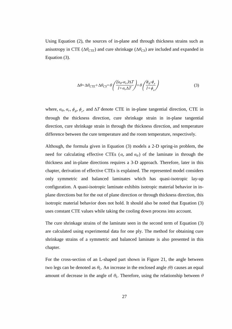
For the cross-section of an L-shaped part shown in Figure 21, the angle between
two legs can be denoted as L. An increase in the enclosed angle causes an equal
amount of decrease in the angle of L. Therefore, using the relationship between
28
and L, Equation (3) can be reorganized to account for the angle L as demonstrated
in Equation (4).
Figure 21: Cross-section of an L shaped part
T
T
(4)
Determining mechanical and thermal properties of a laminate experimentally is not
always feasible since the parameters related to each manufacturing process such as
time, applied temperature and pressure or manufacturing method might differ
considerably. Thus, models have been generated to estimate some mechanical and
thermal properties of composites in different levels such as from micromechanical
level like the fiber-matrix interphase to macromechanical level like laminates. In the
remaining parts of this chapter, a model which predicts three dimensional stiffness
matrix for a symmetric laminate made of UD plies is introduced first [47]. This is
followed by obtaining three dimensional effective CTE values of a symmetric and
balanced laminate by using the method proposed by Dong [44]. Then, a cure
shrinkage model is generated to predict laminate’s shrinkage strain by using
29
experimental data. The results are then implemented in Equation (4) to have a quick
estimation of spring-in angle for a symmetric and balanced laminate.
2.2 3-D EFFECTIVE THERMOMECHANICAL PROPERTIES OF A
SYMMETRIC AND BALANCED LAMINATE
Classical lamination theory (CLT) assumes plane stress solution and ignores
through thickness stresses. It is limited for the analysis of thin plates [33].
Therefore, CLT becomes useless for the cases such as spring-in of corner shaped
geometries where through the thickness effects are important. For that reason, to
predict 3-D effective mechanical properties, averaging methods are used in studies
[47, 48, 49]. In this section, the method represented by Chen and Tsai [47] is
explained in detail and employed for the solution.
2.2.1 Effective Stiffness Matrix
Figure 22 presents a small portion of an L-shaped laminate made of differently
oriented UD plies. There are two different coordinate systems: a local 123-
coordinate system defined on each ply and a global xyz-coordinate system. In each
ply, the 1-axis coincides with the fiber direction and the 2-axis, which is the other
in-plane axis, is perpendicular to the fiber direction. The 3-axis, on the other hand,
is in the through-thickness direction and coincides with global z-axis. For each ply,
fiber reinforcements (or local 1-axis) are oriented at an angle of θ with the global x-
axis.
30
Figure 22: L shaped laminate made of differently oriented UD prepregs [33]
The linear-elastic tensorial constitutive equation defining stress-strain relationship
can be written with respect to the local coordinate system as shown in Equation (5).
(5)
where is the stiffness matrix of an orthotropic (or transversely isotropic) ply and
it is the inverse of the compliance matrix :
(6)
If the fiber arrangement is assumed to be the identical in directions of local 2- and
3-axes, then the material properties may also be assumed to be same in these
directions. These composite materials, such as the ones composed of perfectly
aligned UD, plies are called as transversely isotropic. By using the compliance
matrix , strain can be related to stress:
31
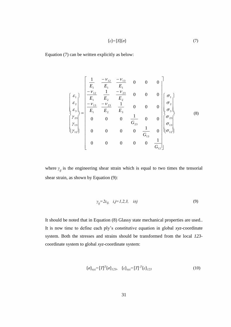
(7)
Equation (7) can be written explicitly as below:
12
13
23
3
2
1
12
13
23
32
23
1
13
2
23
21
12
1
13
1
12
1
12
13
23
3
2
1
100000
01
0000
001
000
0001
0001
0001
G
G
G
EEE
EEE
EEE
(8)
where i is the engineering shear strain which is equal to two times the tensorial
shear strain, as shown by Equation (9):
i i i i (9)
It should be noted that in Equation (8) Glassy state mechanical properties are used..
It is now time to define each ply’s constitutive equation in global xyz-coordinate
system. Both the stresses and strains should be transformed from the local 123-
coordinate system to global xyz-coordinate system:
y T T , y T T (10)
32
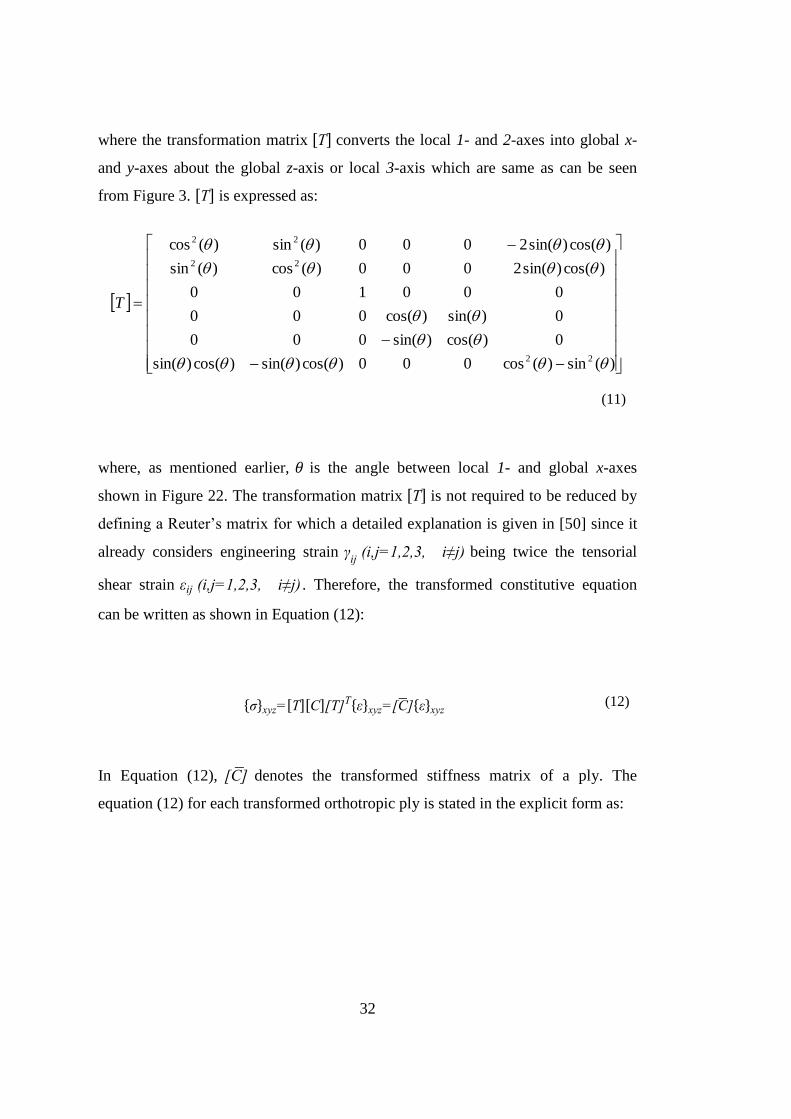
where the transformation matrix T converts the local 1- and 2-axes into global x-
and y-axes about the global z-axis or local 3-axis which are same as can be seen
from Figure 3. T is expressed as:
)(sin)(cos000)cos()sin()cos()sin(
0)cos()sin(000
0)sin()cos(000
000100
)cos()sin(2000)(cos)(sin
)cos()sin(2000)(sin)(cos
22
22
22
T
(11)
where, as mentioned earlier, is the angle between local 1- and global x-axes
shown in Figure 22. The transformation matrix T is not required to be reduced by
defining a Reuter’s matrix for which a detailed explanation is given in [50] since it
already considers engineering strain i i i being twice the tensorial
shear strain i i i . Therefore, the transformed constitutive equation
can be written as shown in Equation (12):
y T T T y y (12)
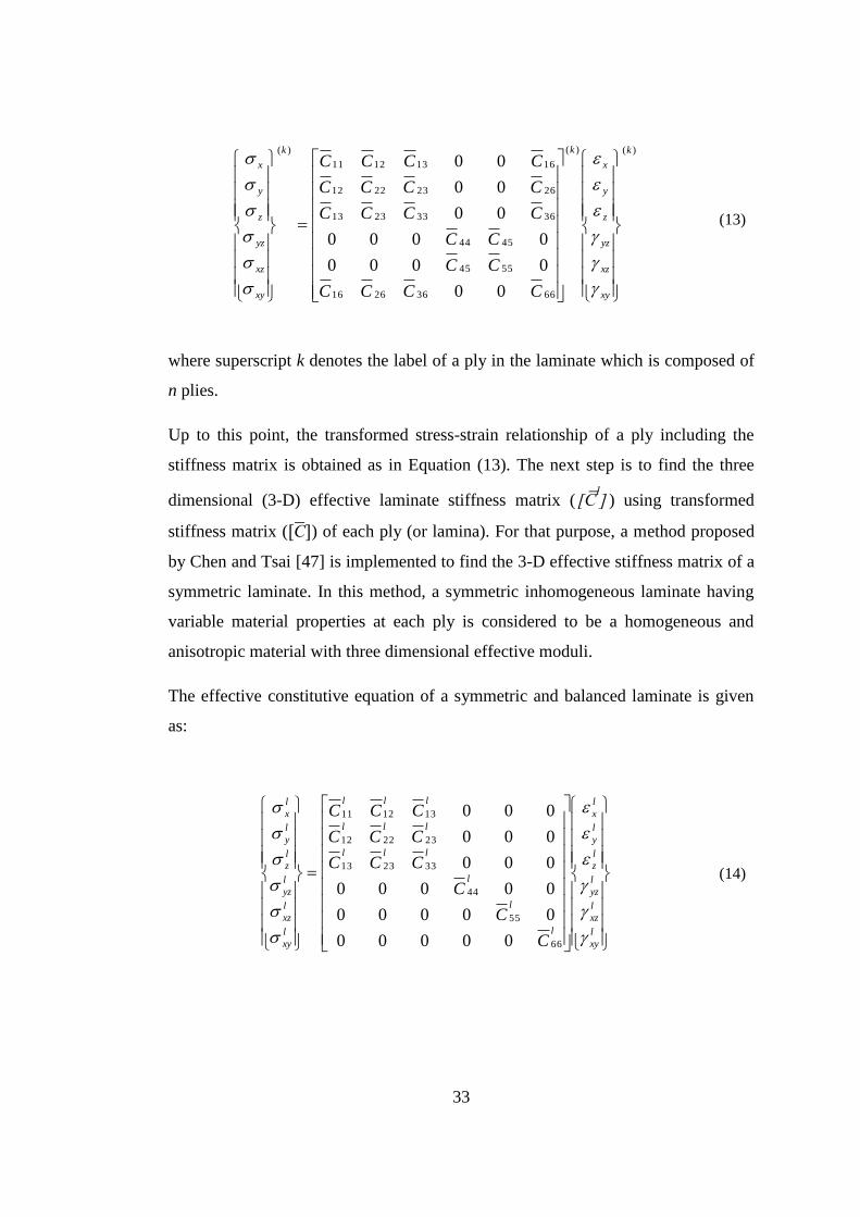
In Equation (12), denotes the transformed stiffness matrix of a ply. The
equation (12) for each transformed orthotropic ply is stated in the explicit form as:
33
)()(
66362616
5545
4544
36332313
26232212
16131211
)(
00
0000
0000
00
00
00k
xy
xz
yz
z
y
x
kk
xy
xz
yz
z
y
x
CCCC
CC
CC
CCCC
CCCC
CCCC
(13)
where superscript k denotes the label of a ply in the laminate which is composed of
n plies.
Up to this point, the transformed stress-strain relationship of a ply including the
stiffness matrix is obtained as in Equation (13). The next step is to find the three
dimensional (3-D) effective laminate stiffness matrix ( ) using transformed
stiffness matrix ( ) of each ply (or lamina). For that purpose, a method proposed
by Chen and Tsai [47] is implemented to find the 3-D effective stiffness matrix of a
symmetric laminate. In this method, a symmetric inhomogeneous laminate having
variable material properties at each ply is considered to be a homogeneous and
anisotropic material with three dimensional effective moduli.
The effective constitutive equation of a symmetric and balanced laminate is given
as:
l
xy
l
xz
l
yz
l
z
l
y
l
x
l
l
l
lll
lll
lll
l
xy
l
xz
l
yz
l
z
l
y
l
x
C
C
C
CCC
CCC
CCC
66
55
44
332313
232212
131211
00000
00000
00000
000
000
000
(14)
34
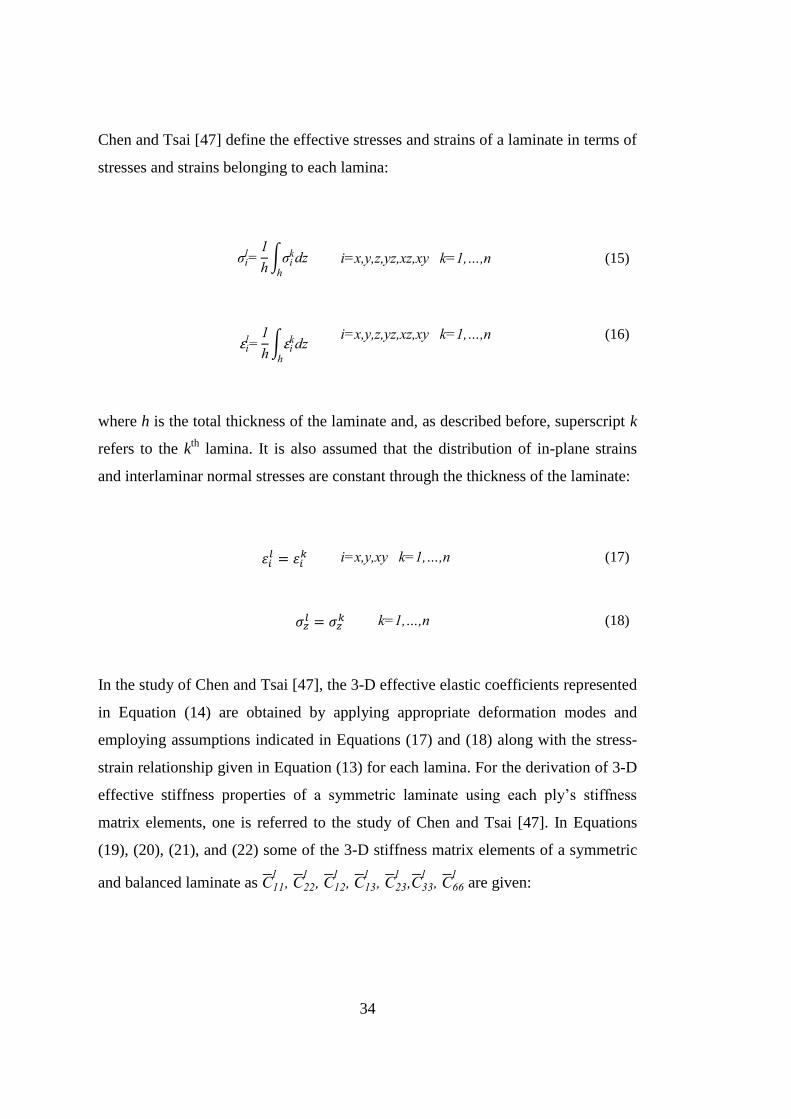
Chen and Tsai [47] define the effective stresses and strains of a laminate in terms of
stresses and strains belonging to each lamina:
i
i
i y y y … n (15)
i
i
i y y y … n (16)
where h is the total thickness of the laminate and, as described before, superscript k
refers to the kth
lamina. It is also assumed that the distribution of in-plane strains
and interlaminar normal stresses are constant through the thickness of the laminate:
i y y … n (17)
… n (18)
In the study of Chen and Tsai [47], the 3-D effective elastic coefficients represented
in Equation (14) are obtained by applying appropriate deformation modes and
employing assumptions indicated in Equations (17) and (18) along with the stress-
strain relationship given in Equation (13) for each lamina. For the derivation of 3-D
effective stiffness properties of a symmetric laminate using each ply’s stiffness
matrix elements, one is referred to the study of Chen and Tsai [47]. In Equations
(19), (20), (21), and (22) some of the 3-D stiffness matrix elements of a symmetric
and balanced laminate as
are given:
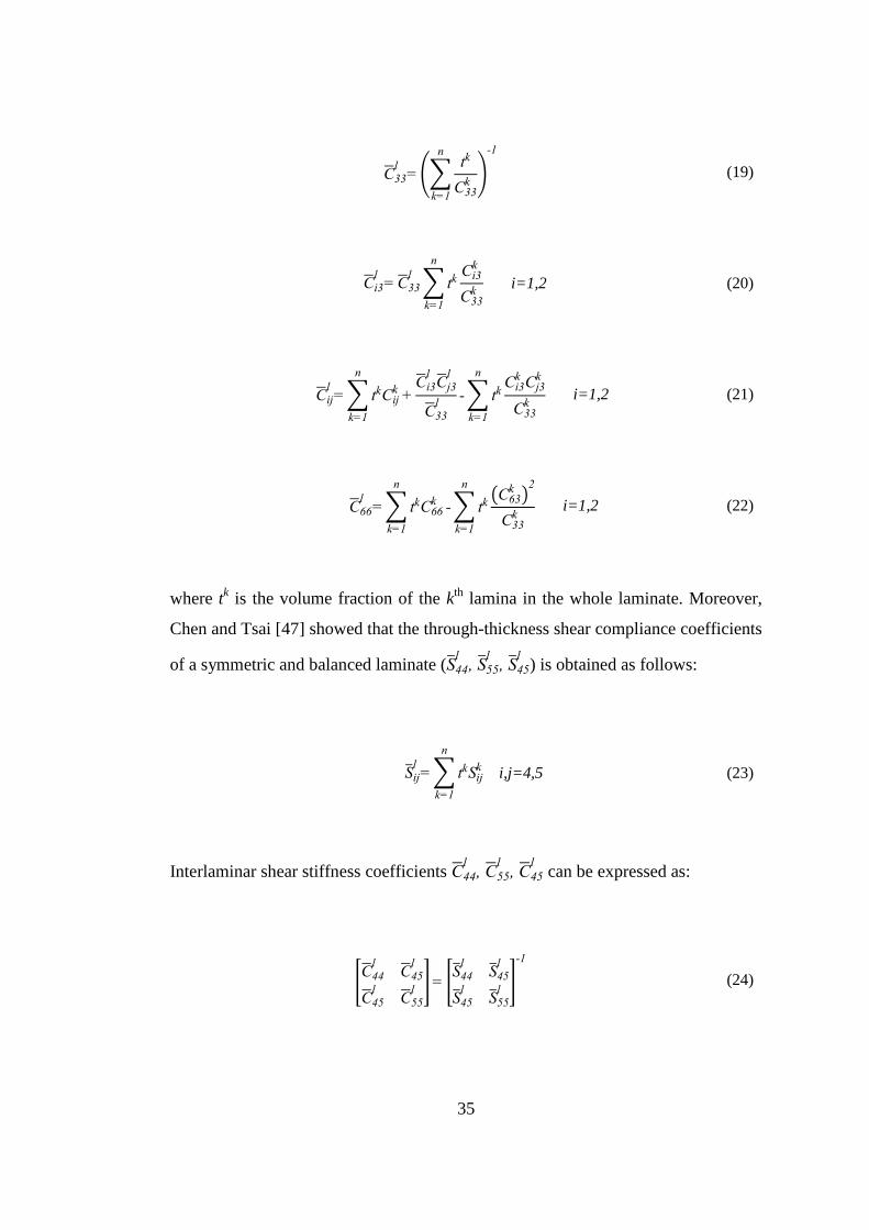
35
n
(19)
i
i
n
i=1,2 (20)
i i
n
i
i
n
i=1,2 (21)
n
n
i=1,2 (22)
where tk is the volume fraction of the k
th lamina in the whole laminate. Moreover,
Chen and Tsai [47] showed that the through-thickness shear compliance coefficients
of a symmetric and balanced laminate (
) is obtained as follows:
i i
n
i,j=4,5 (23)
Interlaminar shear stiffness coefficients
can be expressed as:
(24)

36
However, in a symmetric and balanced laminate, the individual plies occur in
pairs. Due to this reason, by combining Equations (8), (11), (13), (23), it can be
concluded that
becomes zero for a symmetric and balanced laminate. This
means that:
(25)
where
can be calculated using Equation (23).
2.2.2 Effective Coefficient of Thermal Expansions (CTEs)
The strains in a ply include thermal and mechanical components as shown in
Equation (26):
y y
y
T (26)
where stands for the mechanical component of the strain, consists of the
CTEs in vectorial form, T denotes the difference between the cure temperature and
room temperature. For an orthotropic ply (or lamina), the CTEs in local 123-
coordinate system can be transferred to the global xyz-coordinate system with the
help of transformation matrix [T] which is represented in Equation (11):

37
0
0
0
0
0
3
2
1
T
xy
z
y
x
T (27)
When there is no mechanical load applied and only thermal stresses are considered,
the constitutive relationship for a ply oriented at an angle of given in Equation
(13) becomes:
)()()(
66362616
5545
4544
36332313
26232212
16131211
0
0
0
0
0
0
200
0000
0000
00
00
00kk
xyxy
xz
yz
zz
yy
xx
k
T
T
T
T
CCCC
CC
CC
CCCC
CQQQ
CCCC
(28)
Equation (28) can be rearranged as:
T
CCCC
CCCC
CCCC
CCCC
CCCC
CC
CC
CCCC
CCCC
CCCC
xyzyx
xyzyx
xyzyx
xyzyx
k
xy
xz
yz
z
y
x
k
66362616
36332313
26232212
16131211)()(
66362616
5545
4544
36332313
26232212
16131211
2
0
0
2
2
2
00
0000
0000
00
00
00
(29)
As given in Equation (17), Dong [44] assumes that all plies are bonded strictly to
each other and they have the same strains. This means that strains of a laminated
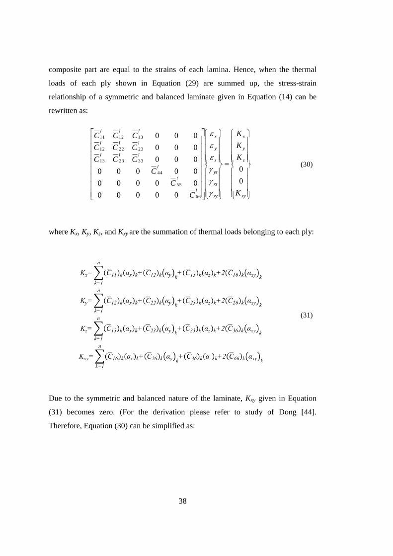
38
composite part are equal to the strains of each lamina. Hence, when the thermal
loads of each ply shown in Equation (29) are summed up, the stress-strain
relationship of a symmetric and balanced laminate given in Equation (14) can be
rewritten as:
xy
z
y
x
xy
xz
yz
z
y
x
l
l
l
lll
lll
lll
K
K
K
K
C
C
C
CCC
CCC
CCC
0
0
00000
00000
00000
000
000
000
66
55
44
332313
232212
131211
(30)
where Kx, Ky, Kz, and Kxy are the summation of thermal loads belonging to each ply:
y y
n
y y y
n
y y
n
y y y
n
(31)
Due to the symmetric and balanced nature of the laminate, Kxy given in Equation
(31) becomes zero. (For the derivation please refer to study of Dong [44].
Therefore, Equation (30) can be simplified as:
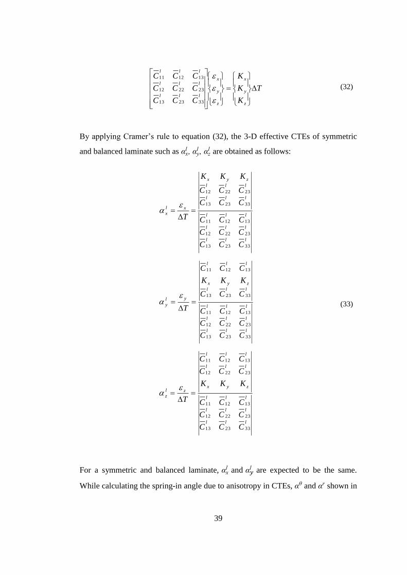
39
T
K
K
K
CCC
CCC
CCC
z
y
x
z
y
x
lll
lll
lll
332313
232212
131211
(32)
By applying Cramer’s rule to equation (32), the 3-D effective CTEs of symmetric
and balanced laminate such as y
are obtained as follows:
lll
lll
lll
lll
lll
zyx
xl
x
CCC
CCC
CCC
CCC
CCC
KKK
T
332313
232212
131211
332313
232212
lll
lll
lll
lll
zyx
lll
yl
y
CCC
CCC
CCC
CCC
KKK
CCC
T
332313
232212
131211
332313
131211
lll
lll
lll
zyx
lll
lll
zl
z
CCC
CCC
CCC
KKK
CCC
CCC
T
332313
232212
131211
232212
131211
(33)
For a symmetric and balanced laminate, and
are expected to be the same.
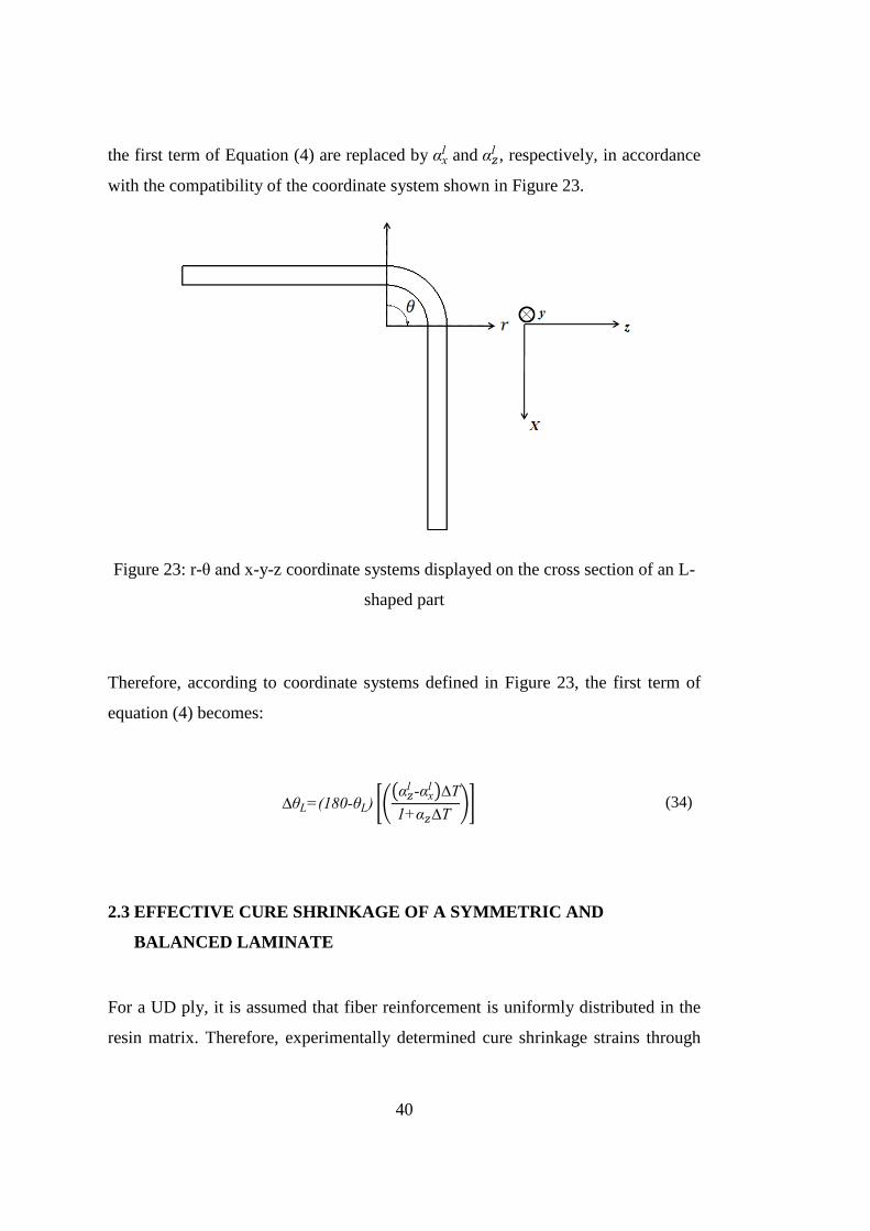
While calculating the spring-in angle due to anisotropy in CTEs, and shown in
40
the first term of Equation (4) are replaced by and
, respectively, in accordance
with the compatibility of the coordinate system shown in Figure 23.
Figure 23: r-θ and x-y-z coordinate systems displayed on the cross section of an L-
shaped part
Therefore, according to coordinate systems defined in Figure 23, the first term of
equation (4) becomes:
T
T (34)
2.3 EFFECTIVE CURE SHRINKAGE OF A SYMMETRIC AND
BALANCED LAMINATE
For a UD ply, it is assumed that fiber reinforcement is uniformly distributed in the
resin matrix. Therefore, experimentally determined cure shrinkage strains through
41
the resin dominant transverse directions, namely 2- and 3-directions in the local
coordinate system shown in Figure 22, can be treated as the same. (i.e. c
c )
However, in the longitudinal direction or in the local 1-direction, due to fiber
reinforcement, lamina is subjected to very little cure shrinkage which can be
regarded as zero, (i.e., c ) [51].
It can be considered that each ply in a laminate is subjected to the same amount of
cure shrinkage in through the thickness direction, therefore; they contract equally in
this direction. Consequently, effective through-thickness cure shrinkage strain ( )
of a laminate can be written as:
c
n
(35)
where is the volume fraction of the kth
ply (or lamina). On the other hand, the in–
plane cure shrinkage strain of a laminate ( ) due to transverse cure shrinkage
strains ( c ) of each lamina can be written as follows:
c co
n
(36)
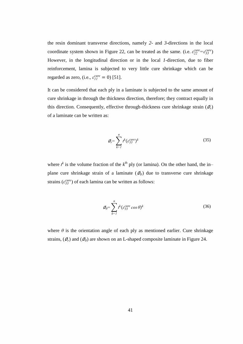
where is the orientation angle of each ply as mentioned earlier. Cure shrinkage
strains, ( ) and ( ) are shown on an L-shaped composite laminate in Figure 24.
42
Figure 24: Cure shrinkage strains ( ) and ( ) with the corresponding r-θ
coordinate system displayed on an L-shaped part
2.4 MATERIAL PROPERTIES NEEDED FOR THE CALCULATION OF
SPRING-IN ANGLE
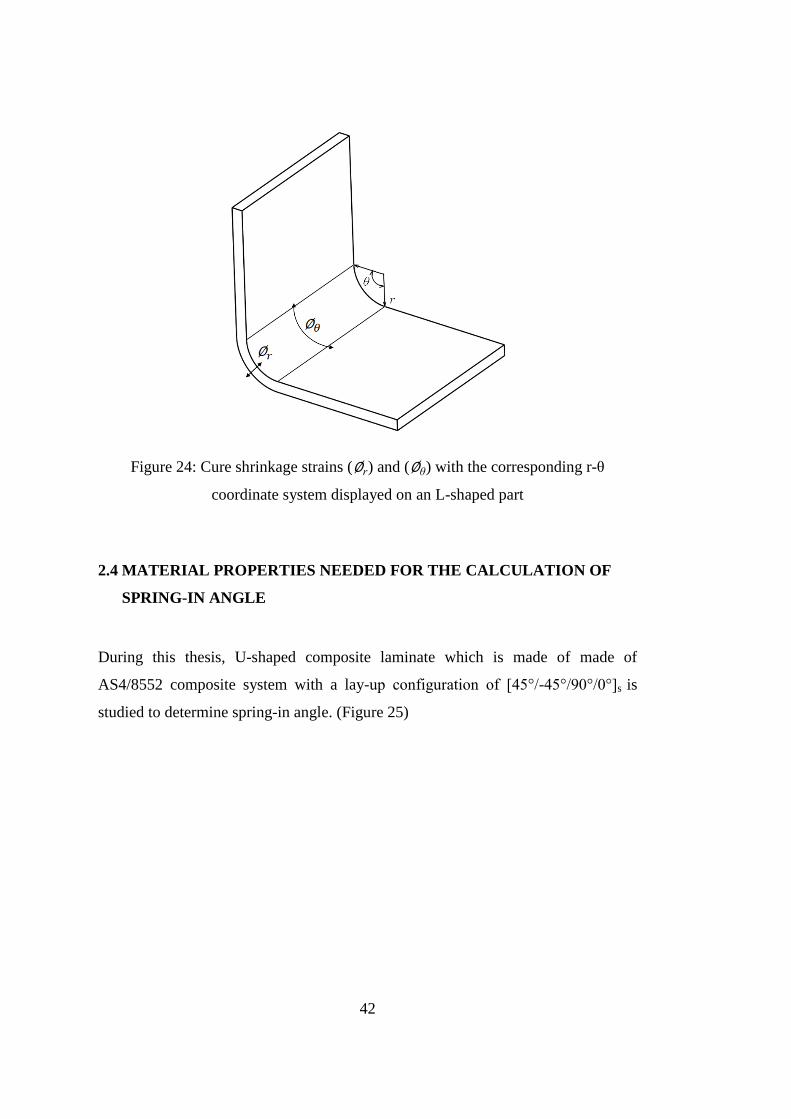
During this thesis, U-shaped composite laminate which is made of made of
AS4/8552 composite system with a lay-up configuration of [45°/-45°/90°/0°]s is
studied to determine spring-in angle. (Figure 25)
43
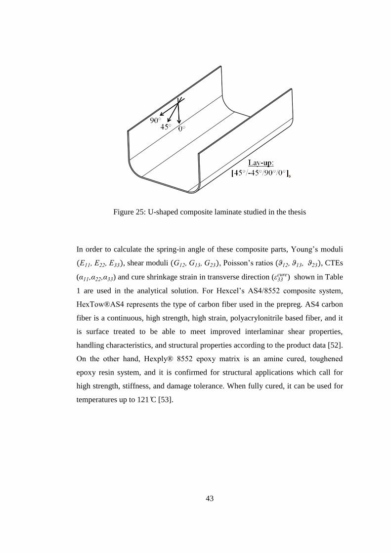
Figure 25: U-shaped composite laminate studied in the thesis
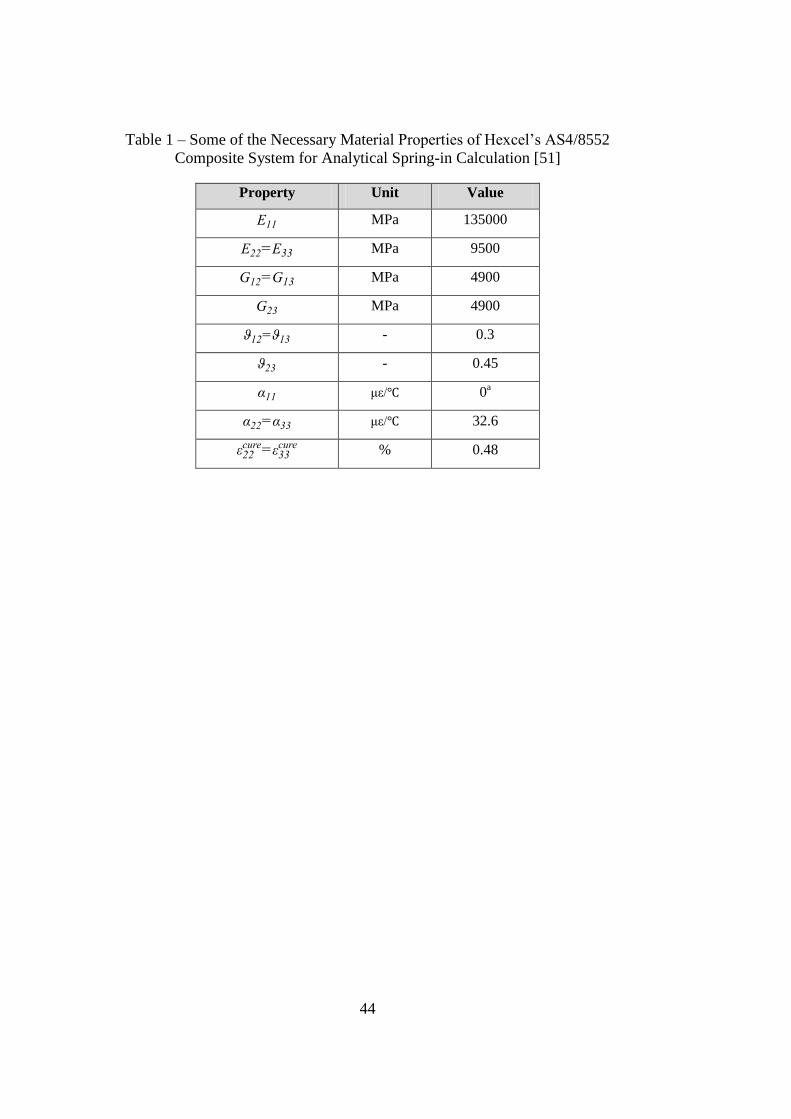
In order to calculate the spring-in angle of these composite parts, Young’s moduli
, shear moduli , Poisson’s ratios , CTEs
( ) and cure shrinkage strain in transverse direction ( c ) shown in Table
1 are used in the analytical solution. For Hexcel’s AS4/8552 composite system,
HexTow®AS4 represents the type of carbon fiber used in the prepreg. AS4 carbon
fiber is a continuous, high strength, high strain, polyacrylonitrile based fiber, and it
is surface treated to be able to meet improved interlaminar shear properties,
handling characteristics, and structural properties according to the product data [52].
On the other hand, Hexply® 8552 epoxy matrix is an amine cured, toughened
epoxy resin system, and it is confirmed for structural applications which call for
high strength, stiffness, and damage tolerance. When fully cured, it can be used for
temperatures up to 121 C [53].
44
Table 1 – Some of the Necessary Material Properties of Hexcel’s AS4/8552
Composite System for Analytical Spring-in Calculation [51]
Property Unit Value
MPa 135000
MPa 9500
MPa 4900
MPa 4900
- 0.3
- 0.45
μ / 0a
μ / 32.6
c
c % 0.48
45
CHAPTER 3
EXPERIMENTAL INVESTIGATION OF SPRING-IN
A number of U-shaped composite laminates consisting of UD plies has been
manufactured via autoclave forming process in order to investigate the spring-in
problem experimentally. Surface temperature of the tool-part assembly has been
monitored during the complete cure cycle by using thermocouples and the spring-in
measurement for the manufactured parts has been conducted using an optical
scanning device after completion of the manufacturing process. The details related
to autoclave forming process including the cure cycle, thermocouple installations
for temperature measurements and the spring-in measurement are presented in this
chapter.
3.1. LAY-UP CONFIGURATION, MATERIAL TYPE AND DIMENSIONS
Designing a laminate with symmetric and balanced configuration prevents warpage
formation by cancelling out the bending effects of thermal and cure strains. On the
other hand, for laminates having corner shaped geometries such as U-shaped
composite parts manufactured within the scope of this thesis, spring-in problem will
still be present even though the laminates have symmetric and balanced lay-up
configuration mainly because of anisotropy in CTEs and other factors like tool-part
interaction and cure shrinkage. Therefore, to minimize warpage problem and not to
have “warpage and spring-in” couplings in the manufactured composite parts, a
symmetric and balanced lay-up configuration is considered. Quasi-isotropic
laminate configuration that is studied in the thesis is taken as [45°/-45°/90°/0°]s.
Hexcel’s UD carbon-epoxy prepreg (AS4/8552) is used to manufacture U-shaped
composite parts with autoclave manufacturing technique. Details related to
AS4/8552 composite system have already been explained in the previous chapter.
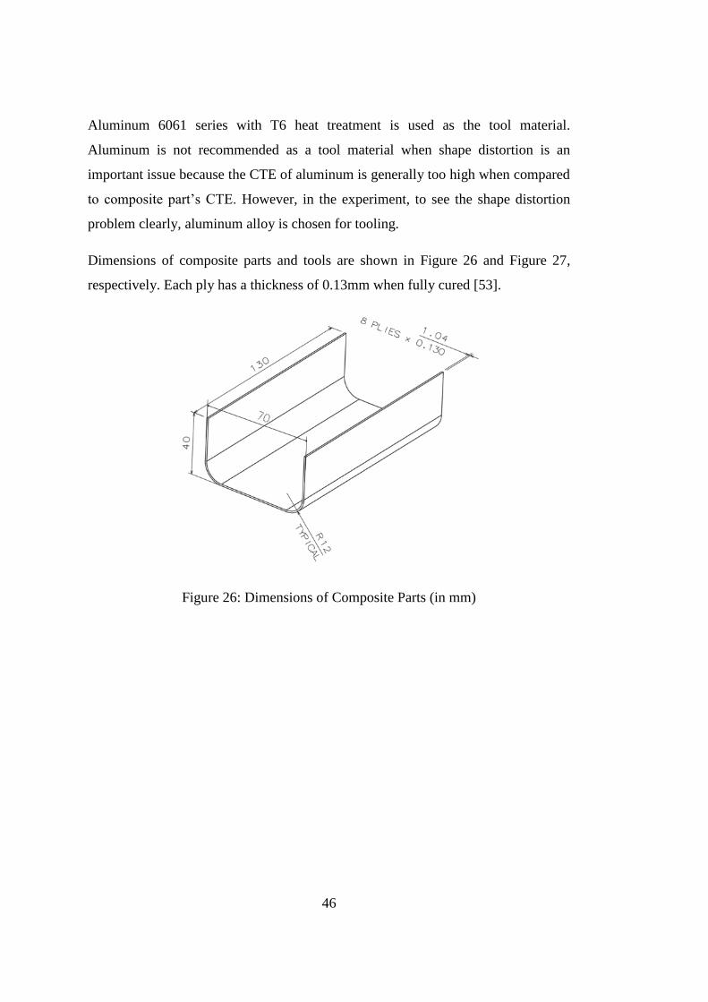
46
Aluminum 6061 series with T6 heat treatment is used as the tool material.
Aluminum is not recommended as a tool material when shape distortion is an
important issue because the CTE of aluminum is generally too high when compared
to composite part’s CTE. However, in the experiment, to see the shape distortion
problem clearly, aluminum alloy is chosen for tooling.
Dimensions of composite parts and tools are shown in Figure 26 and Figure 27,
respectively. Each ply has a thickness of 0.13mm when fully cured [53].
Figure 26: Dimensions of Composite Parts (in mm)
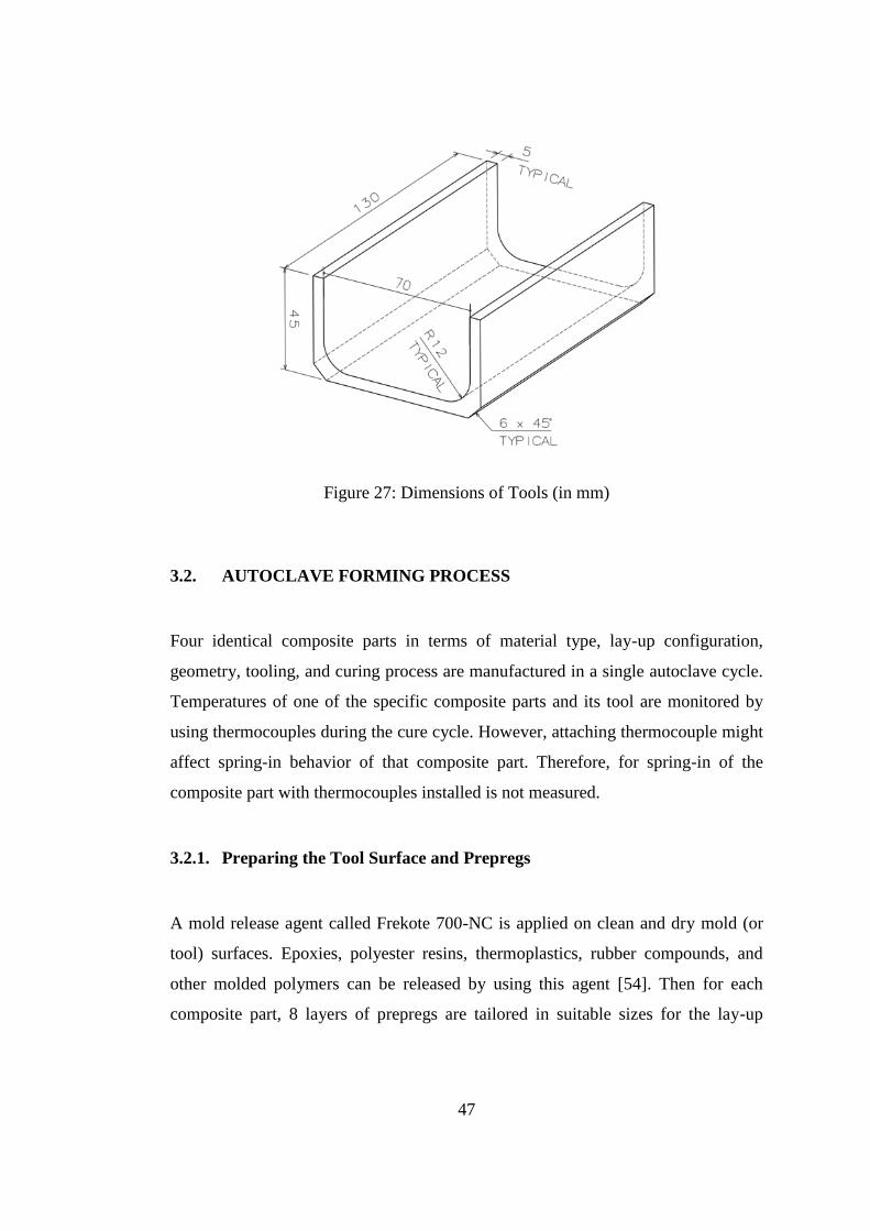
47
Figure 27: Dimensions of Tools (in mm)
3.2. AUTOCLAVE FORMING PROCESS
Four identical composite parts in terms of material type, lay-up configuration,
geometry, tooling, and curing process are manufactured in a single autoclave cycle.
Temperatures of one of the specific composite parts and its tool are monitored by
using thermocouples during the cure cycle. However, attaching thermocouple might
affect spring-in behavior of that composite part. Therefore, for spring-in of the
composite part with thermocouples installed is not measured.
3.2.1. Preparing the Tool Surface and Prepregs
A mold release agent called Frekote 700-NC is applied on clean and dry mold (or
tool) surfaces. Epoxies, polyester resins, thermoplastics, rubber compounds, and
other molded polymers can be released by using this agent [54]. Then for each
composite part, 8 layers of prepregs are tailored in suitable sizes for the lay-up
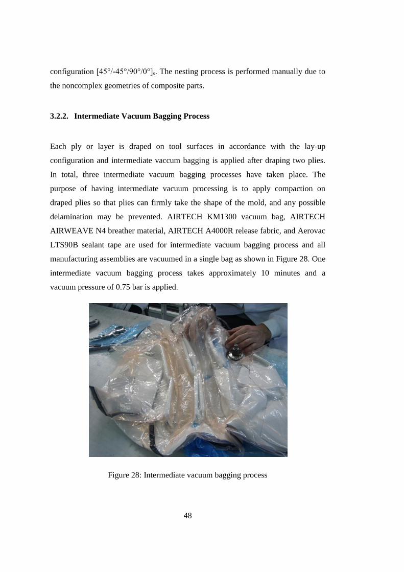
48
configuration [45°/-45°/90°/0°]s. The nesting process is performed manually due to
the noncomplex geometries of composite parts.
3.2.2. Intermediate Vacuum Bagging Process
Each ply or layer is draped on tool surfaces in accordance with the lay-up
configuration and intermediate vaccum bagging is applied after draping two plies.
In total, three intermediate vacuum bagging processes have taken place. The
purpose of having intermediate vacuum processing is to apply compaction on
draped plies so that plies can firmly take the shape of the mold, and any possible
delamination may be prevented. AIRTECH KM1300 vacuum bag, AIRTECH
AIRWEAVE N4 breather material, AIRTECH A4000R release fabric, and Aerovac
LTS90B sealant tape are used for intermediate vacuum bagging process and all
manufacturing assemblies are vacuumed in a single bag as shown in Figure 28. One
intermediate vacuum bagging process takes approximately 10 minutes and a
vacuum pressure of 0.75 bar is applied.
Figure 28: Intermediate vacuum bagging process
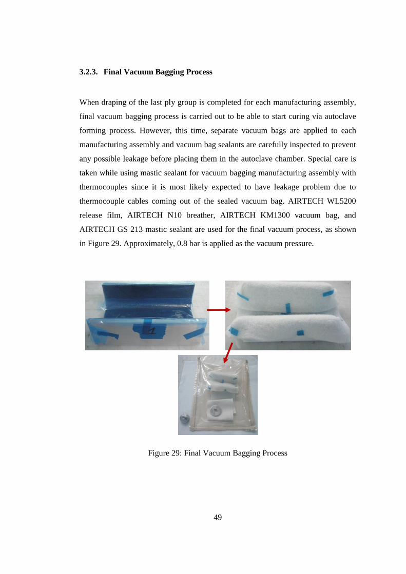
49
3.2.3. Final Vacuum Bagging Process
When draping of the last ply group is completed for each manufacturing assembly,
final vacuum bagging process is carried out to be able to start curing via autoclave
forming process. However, this time, separate vacuum bags are applied to each
manufacturing assembly and vacuum bag sealants are carefully inspected to prevent
any possible leakage before placing them in the autoclave chamber. Special care is
taken while using mastic sealant for vacuum bagging manufacturing assembly with
thermocouples since it is most likely expected to have leakage problem due to
thermocouple cables coming out of the sealed vacuum bag. AIRTECH WL5200
release film, AIRTECH N10 breather, AIRTECH KM1300 vacuum bag, and
AIRTECH GS 213 mastic sealant are used for the final vacuum process, as shown
in Figure 29. Approximately, 0.8 bar is applied as the vacuum pressure.
Figure 29: Final Vacuum Bagging Process
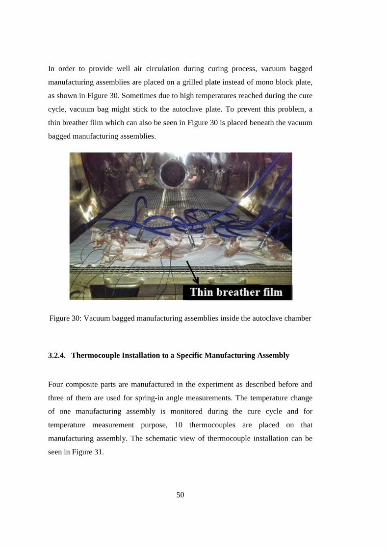
50
In order to provide well air circulation during curing process, vacuum bagged
manufacturing assemblies are placed on a grilled plate instead of mono block plate,
as shown in Figure 30. Sometimes due to high temperatures reached during the cure
cycle, vacuum bag might stick to the autoclave plate. To prevent this problem, a
thin breather film which can also be seen in Figure 30 is placed beneath the vacuum
bagged manufacturing assemblies.
Figure 30: Vacuum bagged manufacturing assemblies inside the autoclave chamber
3.2.4. Thermocouple Installation to a Specific Manufacturing Assembly
Four composite parts are manufactured in the experiment as described before and
three of them are used for spring-in angle measurements. The temperature change
of one manufacturing assembly is monitored during the cure cycle and for
temperature measurement purpose, 10 thermocouples are placed on that
manufacturing assembly. The schematic view of thermocouple installation can be
seen in Figure 31.
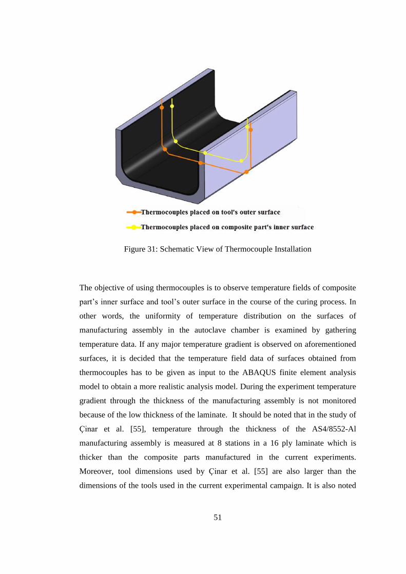
51
Figure 31: Schematic View of Thermocouple Installation
The objective of using thermocouples is to observe temperature fields of composite
part’s inner surface and tool’s outer surface in the course of the curing process. In
other words, the uniformity of temperature distribution on the surfaces of
manufacturing assembly in the autoclave chamber is examined by gathering
temperature data. If any major temperature gradient is observed on aforementioned
surfaces, it is decided that the temperature field data of surfaces obtained from
thermocouples has to be given as input to the ABAQUS finite element analysis
model to obtain a more realistic analysis model. During the experiment temperature
gradient through the thickness of the manufacturing assembly is not monitored
because of the low thickness of the laminate. It should be noted that in the study of
Çinar et al. [55], temperature through the thickness of the AS4/8552-Al
manufacturing assembly is measured at 8 stations in a 16 ply laminate which is
thicker than the composite parts manufactured in the current experiments.
Moreover, tool dimensions used by Çinar et al. [55] are also larger than the
dimensions of the tools used in the current experimental campaign. It is also noted
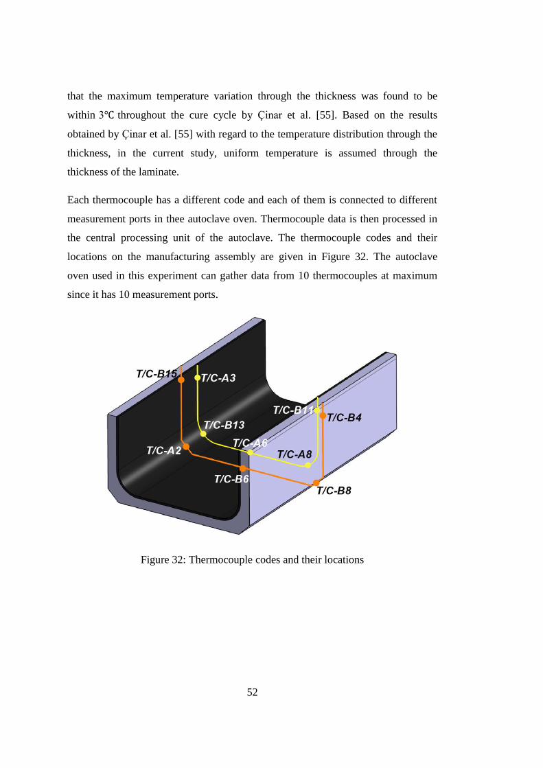
52
that the maximum temperature variation through the thickness was found to be
within 3 throughout the cure cycle by Çinar et al. [55]. Based on the results
obtained by Çinar et al. [55] with regard to the temperature distribution through the
thickness, in the current study, uniform temperature is assumed through the
thickness of the laminate.
Each thermocouple has a different code and each of them is connected to different
measurement ports in thee autoclave oven. Thermocouple data is then processed in
the central processing unit of the autoclave. The thermocouple codes and their
locations on the manufacturing assembly are given in Figure 32. The autoclave
oven used in this experiment can gather data from 10 thermocouples at maximum
since it has 10 measurement ports.
Figure 32: Thermocouple codes and their locations
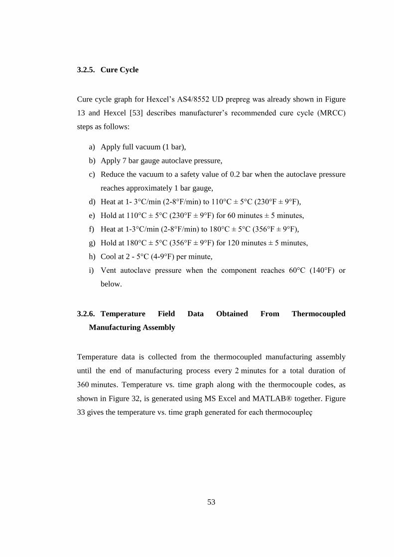
53
3.2.5. Cure Cycle
Cure cycle graph for Hexcel’s AS4/8552 UD prepreg was already shown in Figure
13 and Hexcel [53] describes manufacturer’s recommended cure cycle (MRCC)
steps as follows:
a) Apply full vacuum (1 bar),
b) Apply 7 bar gauge autoclave pressure,
c) Reduce the vacuum to a safety value of 0.2 bar when the autoclave pressure
reaches approximately 1 bar gauge,
d) Heat at 1- 3°C/min (2-8°F/min) to 110°C ± 5°C (230°F ± 9°F),
e) Hold at 110°C ± 5°C (230°F ± 9°F) for 60 minutes ± 5 minutes,
f) Heat at 1-3°C/min (2-8°F/min) to 180°C ± 5°C (356°F ± 9°F),
g) Hold at 180°C ± 5°C (356°F ± 9°F) for 120 minutes ± 5 minutes,
h) Cool at 2 - 5°C (4-9°F) per minute,
i) Vent autoclave pressure when the component reaches 60°C (140°F) or
below.
3.2.6. Temperature Field Data Obtained From Thermocoupled
Manufacturing Assembly
Temperature data is collected from the thermocoupled manufacturing assembly
until the end of manufacturing process every 2 minutes for a total duration of
360 minutes. Temperature vs. time graph along with the thermocouple codes, as
shown in Figure 32, is generated using MS Excel and MATLAB® together. Figure
33 gives the temperature vs. time graph generated for each thermocoupleç
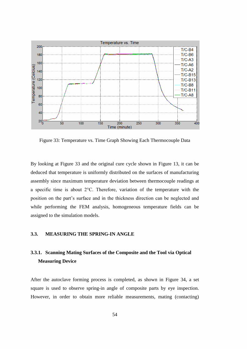
54
Figure 33: Temperature vs. Time Graph Showing Each Thermocouple Data
By looking at Figure 33 and the original cure cycle shown in Figure 13, it can be
deduced that temperature is uniformly distributed on the surfaces of manufacturing
assembly since maximum temperature deviation between thermocouple readings at
a specific time is about 2°C. Therefore, variation of the temperature with the
position on the part’s surface and in the thickness direction can be neglected and
while performing the FEM analysis, homogeneous temperature fields can be
assigned to the simulation models.
3.3. MEASURING THE SPRING-IN ANGLE
3.3.1. Scanning Mating Surfaces of the Composite and the Tool via Optical
Measuring Device
After the autoclave forming process is completed, as shown in Figure 34, a set
square is used to observe spring-in angle of composite parts by eye inspection.
However, in order to obtain more reliable measurements, mating (contacting)
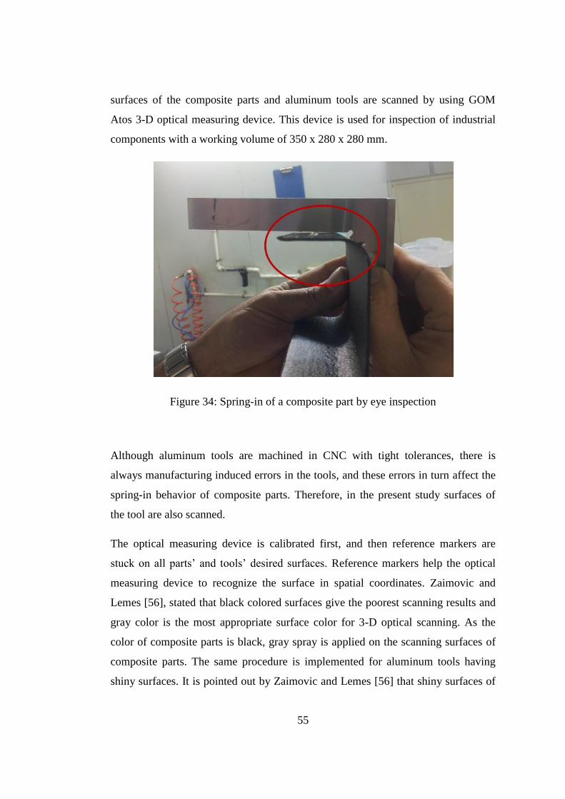
55
surfaces of the composite parts and aluminum tools are scanned by using GOM
Atos 3-D optical measuring device. This device is used for inspection of industrial
components with a working volume of 350 x 280 x 280 mm.
Figure 34: Spring-in of a composite part by eye inspection
Although aluminum tools are machined in CNC with tight tolerances, there is
always manufacturing induced errors in the tools, and these errors in turn affect the
spring-in behavior of composite parts. Therefore, in the present study surfaces of
the tool are also scanned.
The optical measuring device is calibrated first, and then reference markers are
stuck on all parts’ and tools’ desired surfaces. Reference markers help the optical
measuring device to recognize the surface in spatial coordinates. Zaimovic and
Lemes [56], stated that black colored surfaces give the poorest scanning results and
gray color is the most appropriate surface color for 3-D optical scanning. As the
color of composite parts is black, gray spray is applied on the scanning surfaces of
composite parts. The same procedure is implemented for aluminum tools having
shiny surfaces. It is pointed out by Zaimovic and Lemes [56] that shiny surfaces of
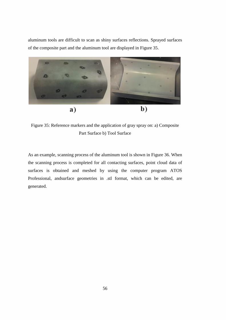
56
aluminum tools are difficult to scan as shiny surfaces reflections. Sprayed surfaces
of the composite part and the aluminum tool are displayed in Figure 35.
Figure 35: Reference markers and the application of gray spray on: a) Composite
Part Surface b) Tool Surface
As an example, scanning process of the aluminum tool is shown in Figure 36. When
the scanning process is completed for all contacting surfaces, point cloud data of
surfaces is obtained and meshed by using the computer program ATOS
Professional, andsurface geometries in .stl format, which can be edited, are
generated.
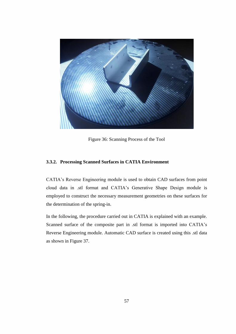
57
Figure 36: Scanning Process of the Tool
3.3.2. Processing Scanned Surfaces in CATIA Environment
CATIA’s Reverse Engineering module is used to obtain CAD surfaces from point
cloud data in .stl format and CATIA’s Generative Shape Design module is
employed to construct the necessary measurement geometries on these surfaces for
the determination of the spring-in.
In the following, the procedure carried out in CATIA is explained with an example.
Scanned surface of the composite part in .stl format is imported into CATIA’s
Reverse Engineering module. Automatic CAD surface is created using this .stl data
as shown in Figure 37.
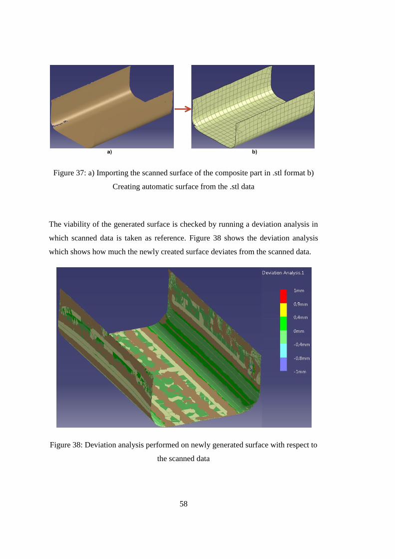
58
Figure 37: a) Importing the scanned surface of the composite part in .stl format b)
Creating automatic surface from the .stl data
The viability of the generated surface is checked by running a deviation analysis in
which scanned data is taken as reference. Figure 38 shows the deviation analysis
which shows how much the newly created surface deviates from the scanned data.
Figure 38: Deviation analysis performed on newly generated surface with respect to
the scanned data
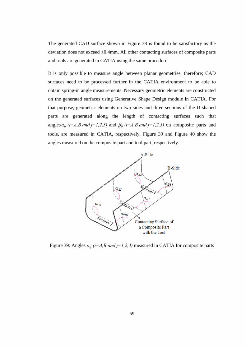
59
The generated CAD surface shown in Figure 38 is found to be satisfactory as the
deviation does not exceed ±0.4mm. All other contacting surfaces of composite parts
and tools are generated in CATIA using the same procedure.
It is only possible to measure angle between planar geometries, therefore; CAD
surfaces need to be processed further in the CATIA environment to be able to
obtain spring-in angle measurements. Necessary geometric elements are constructed
on the generated surfaces using Generative Shape Design module in CATIA. For
that purpose, geometric elements on two sides and three sections of the U shaped
parts are generated along the length of contacting surfaces such that
angles i i an and i i an on composite parts and
tools, are measured in CATIA, respectively. Figure 39 and Figure 40 show the
angles measured on the composite part and tool part, respectively.
Figure 39: Angles i i an measured in CATIA for composite parts
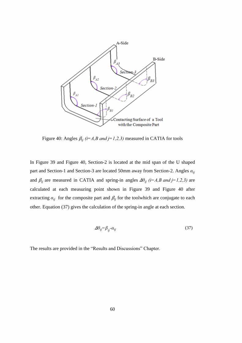
60
Figure 40: Angles i i an measured in CATIA for tools
In Figure 39 and Figure 40, Section-2 is located at the mid span of the U shaped
part and Section-1 and Section-3 are located 50mm away from Section-2. Angles i
and i are measured in CATIA and spring-in angles i i an are
calculated at each measuring point shown in Figure 39 and Figure 40 after
extracting i for the composite part and i for the toolwhich are conjugate to each
other. Equation (37) gives the calculation of the spring-in angle at each section.
i i i (37)
The results are provided in the “Results and Discussions” Chapter.
61
CHAPTER 4
NUMERICAL ANALYSIS MODEL FOR SPRING-IN SIMULATION
For numerical analysis of spring-in, the material properties of the composite are
needed. For material characterization of thermoset composite, cure kinetics models
which predict the trend of cure and state transformations of resin such as gelation
and vitrification are generated. Via these models, material properties such as glass
transition temperature, modulus development during curing process, and CTEs can
be found. The cure shrinkage can be monitored in the course of curing process [37,
40, 51, 57].
For cure kinetics modeling of a thermoset composite, data is obtained via
experiments using differential scanning calorimeter (DSC), dynamic mechanical
analyzer (DMA) and/or thermal mechanical analyzer (TMA) are conducted. DSC is
used to obtain heat flow measurements of a specimen as a function of temperature,
and these measurements determine the amount of heat needed to raise a specimen’s
temperature to a certain degree. Therefore, the degree of cure (α) in one cycle can
be found by using DSC. DMA, on the other hand, is used to understand the
viscoelastic behavior of polymers in terms of temperature, time, frequency, stress,
atmosphere or a combination of these parameters. Material properties of the
composite system such as glass transition temperature (Tg), CTEs, and cure
shrinkage along the thickness direction can be found by using DMA. Thermal
mechanical analyzer (TMA) which measures the deformation of a specimen under
non-oscillating stress conditions with respect to time and temperature can be used
for determining glass transition temperature (Tg) and CTEs of the composite
material [37, 67].
After performing material characterization, effective mechanisms causing the
spring-in problem should be implemented in the numerical analysis model properly.
Ersoy et al. [58] stated that in any numerical analysis model, effective mechanisms
62
such as tool-part interaction, thermal expansion and contraction, cure shrinkage, and
modulus development should be included to predict the manufacturing distortion
accurately.
4.1. MATERIAL PROPERTIES OF AS4/8552 COMPOSITE SYSTEM AND
ALUMINUM TOOL
The most involved material properties related to the spring-in and the residual stress
modeling are the degree of cure, glass transition temperature, cure shrinkage strains,
thermal expansion coefficients, elastic properties, and the gel point which
instantaneously change during the curing process [51]. However, when a thermal
analysis is preferred, in addition to the aforementioned material properties, thermal
conductivity and specific heat capacity are also needed. As will be explained in
detail, a fully coupled thermal-stress analysis model called as “coupled temperature-
displacement” is generated in ABAQUS since this kind of an analysis is preferred
when mechanical and thermal solutions have strong influences on each other [59].
Obviously, in the course of the curing process, residual stress development is
strongly dependent on temperature changes. In this type of analysis, if needed, heat
transfer such as conduction between composite part and tool, and convection
between manufacturing assembly and autoclave environment can also be considered
and implemented.
Ersoy et al. [51] constructed a cure kinetics model for the AS4/8552 composite
system. Using this cure kinetics model, some of the necessary material properties
for spring-in modeling are determined as constant and average values for both
rubbery and glassy states. The total through the thickness cure shrinkage strain
c , Young’s moduli , shear moduli , Poisson’s
ratios , and CTEs ( ) are obtained in this study. Table 2
summarizes the material properties of Hexcel AS4/8552 composite system required
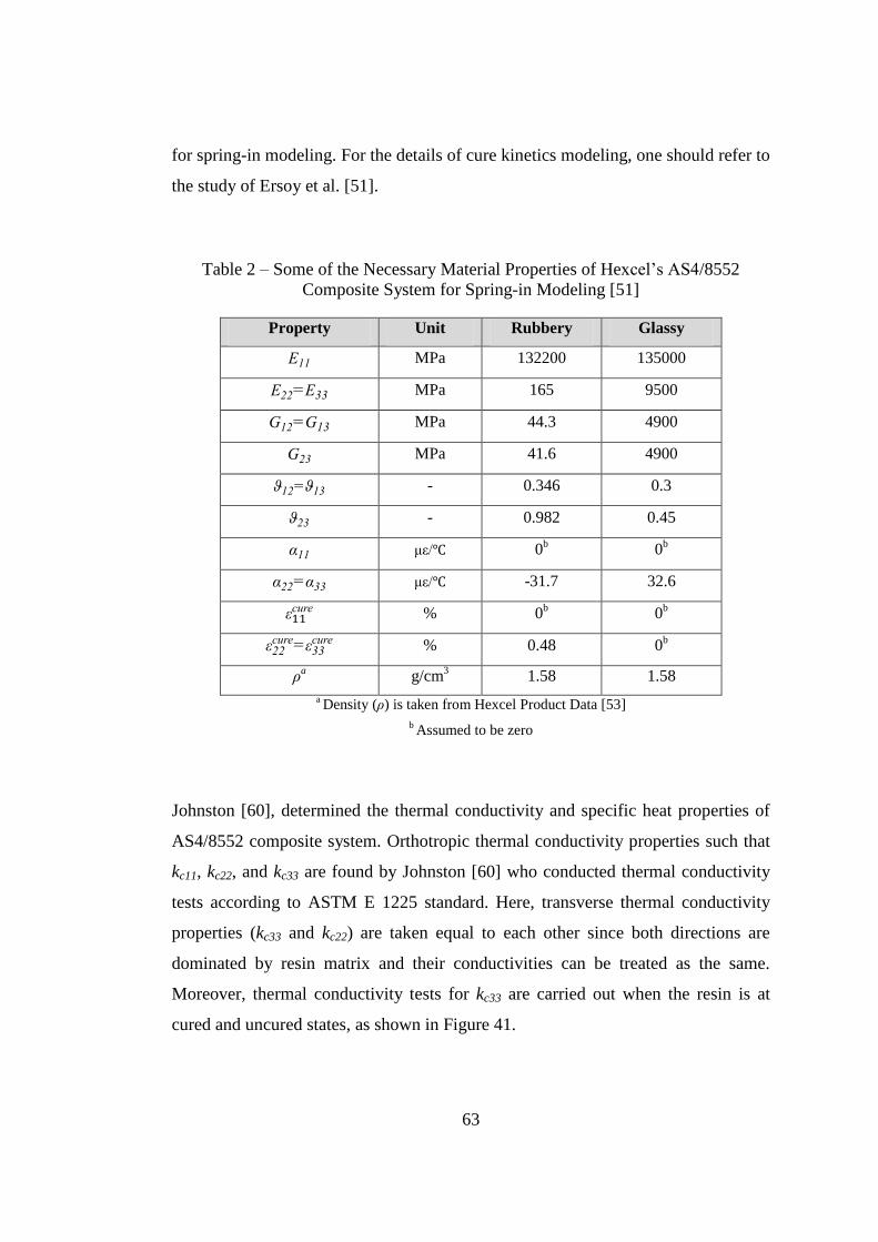
63
for spring-in modeling. For the details of cure kinetics modeling, one should refer to
the study of Ersoy et al. [51].
Table 2 – Some of the Necessary Material Properties of Hexcel’s AS4/8552
Composite System for Spring-in Modeling [51]
Property Unit Rubbery Glassy
MPa 132200 135000
MPa 165 9500
MPa 44.3 4900
MPa 41.6 4900
- 0.346 0.3
- 0.982 0.45
μ / 0b
0b
μ / -31.7 32.6
c % 0
b 0
b
c
c % 0.48 0b
a g/cm
3 1.58 1.58
a Density ( ) is taken from Hexcel Product Data [53]
b Assumed to be zero
Johnston [60], determined the thermal conductivity and specific heat properties of
AS4/8552 composite system. Orthotropic thermal conductivity properties such that
kc11, kc22, and kc33 are found by Johnston [60] who conducted thermal conductivity
tests according to ASTM E 1225 standard. Here, transverse thermal conductivity
properties (kc33 and kc22) are taken equal to each other since both directions are
dominated by resin matrix and their conductivities can be treated as the same.
Moreover, thermal conductivity tests for kc33 are carried out when the resin is at
cured and uncured states, as shown in Figure 41.
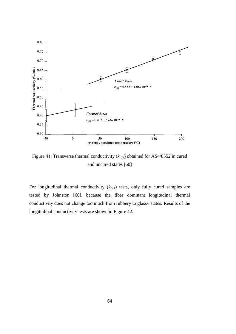
64
Figure 41: Transverse thermal conductivity (kc33) obtained for AS4/8552 in cured
and uncured states [60]
For longitudinal thermal conductivity (kc11) tests, only fully cured samples are
tested by Johnston [60], because the fiber dominant longitudinal thermal
conductivity does not change too much from rubbery to glassy states. Results of the
longitudinal conductivity tests are shown in Figure 42.
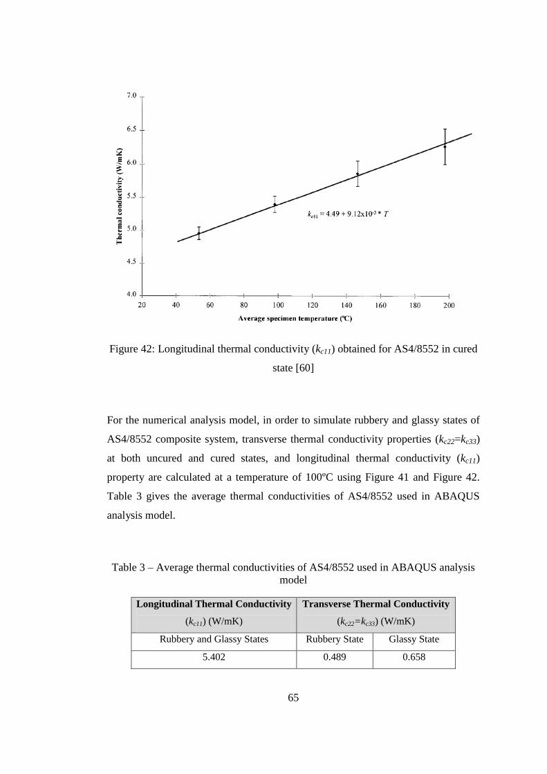
65
Figure 42: Longitudinal thermal conductivity (kc11) obtained for AS4/8552 in cured
state [60]
For the numerical analysis model, in order to simulate rubbery and glassy states of
AS4/8552 composite system, transverse thermal conductivity properties (kc22=kc33)
at both uncured and cured states, and longitudinal thermal conductivity (kc11)
property are calculated at a temperature of 100ºC using Figure 41 and Figure 42.
Table 3 gives the average thermal conductivities of AS4/8552 used in ABAQUS
analysis model.
Table 3 – Average thermal conductivities of AS4/8552 used in ABAQUS analysis
model
Longitudinal Thermal Conductivity
(kc11) (W/mK)
Transverse Thermal Conductivity
(kc22=kc33) (W/mK)
Rubbery and Glassy States Rubbery State Glassy State
5.402 0.489 0.658
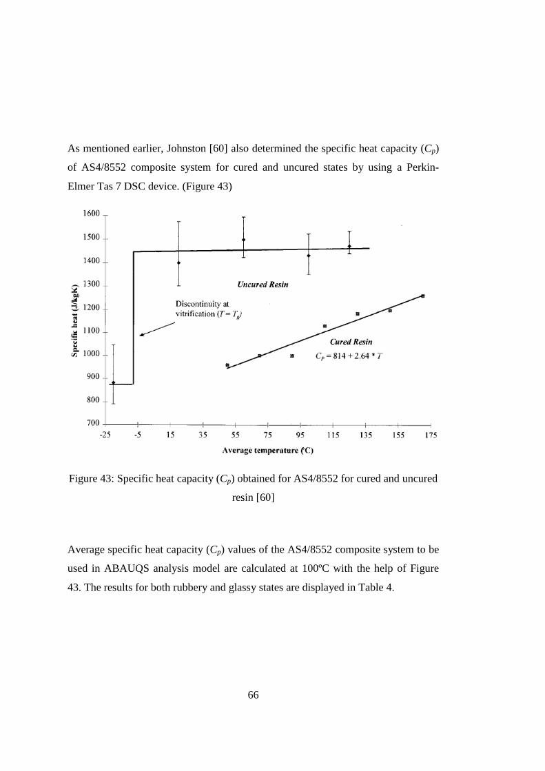
66
As mentioned earlier, Johnston [60] also determined the specific heat capacity (Cp)
of AS4/8552 composite system for cured and uncured states by using a Perkin-
Elmer Tas 7 DSC device. (Figure 43)
Figure 43: Specific heat capacity (Cp) obtained for AS4/8552 for cured and uncured
resin [60]
Average specific heat capacity (Cp) values of the AS4/8552 composite system to be
used in ABAUQS analysis model are calculated at 100ºC with the help of Figure
43. The results for both rubbery and glassy states are displayed in Table 4.
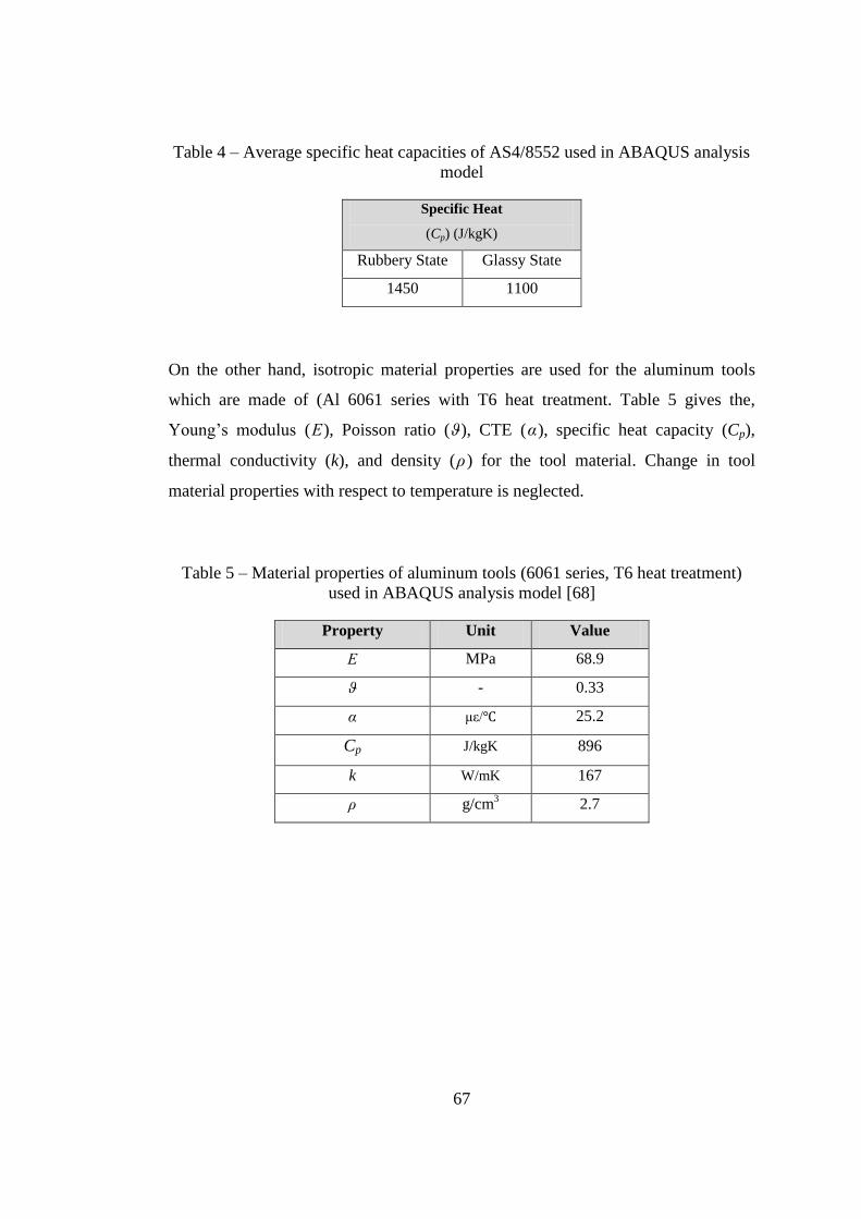
67
Table 4 – Average specific heat capacities of AS4/8552 used in ABAQUS analysis
model
Specific Heat
(Cp) (J/kgK)
Rubbery State Glassy State
1450 1100
On the other hand, isotropic material properties are used for the aluminum tools
which are made of (Al 6061 series with T6 heat treatment. Table 5 gives the,
Young’s modulus ( ), Poisson ratio ( ), CTE ( ), specific heat capacity (Cp),
thermal conductivity (k), and density ( ) for the tool material. Change in tool
material properties with respect to temperature is neglected.
Table 5 – Material properties of aluminum tools (6061 series, T6 heat treatment)
used in ABAQUS analysis model [68]
Property Unit Value
MPa 68.9
- 0.33
μ / 25.2
Cp J/kgK 896
k W/mK 167
g/cm3 2.7
68
4.2. ABAQUS ANALYSIS MODEL
4.2.1. FEM Models in the Literature
In the literature, there are many finite element analysis models simulating shape
distortions of different composite systems [35, 44, 55, 61, 63, 64, 65].
Zhu et al. [61] constructed a transient coupled thermo-chemo-viscoelastic numerical
model which aimed to find the optimal tool geometry. The model generated by Zhu
et al. [61] is a 2-D plane strain finite element in which both warpage and spring-in
problems are considered. First, the effect of composite part’s curvature with
changing CTEs of the tool and then the spring-in problem of the L-shaped
composite part are studied. However, numerical model constructed for the spring-in
problem does not take tool-part interaction into account properly since the
composite part is connected to the tool surface during analysis which means no slip
condition is assumed between tool and composite part.
Dong [44] generated a 3-D FEM model to observe spring-in of an L-shaped
composite part made of T300/CYCOM 934 carbon epoxy unidirectional prepreg.
As an important note, in the study of Dong [44], tool is not constructed for the
numerical model, therefore tool-part interaction is neglected. The model also
considers only the glassy state properties such that viscoelastic behavior of resin is
not taken into account.
In the study of Wiersma et al. [62], first a 3-D numerical composite part model
which is composed of 8-node brick elements is generated. Within this numerical
analysis, only thermoelastic behavior of composite part causing the spring-in is
examined and it is stated that the results of thermoelastic numerical model do not
explain the total spring-in angles found in experiments. Therefore, Wiersma et al.
[62] decided to improve the first numerical modelto include a cure cycle model to
simulate the heat distribution in composite part and a viscoelastic model to include
69
the changes in thermoset resin properties. The extended numerical model generated
by Wiersma et al. [62] is a 2-D model and it also considers tooling effects but no
slip is allowed between tool and part. At the end of the study, it is concluded that
improvement in cure cycle model is needed to have better spring-in angle
predictions and this requires a more complex modeling strategy.
Dong et al. [63] developed a 2-D thermoelastic numerical finite element analysis
(FEA) model by constructing typical structural composite parts such as stiffeners,
corner shaped parts, and cylindrical shells etc... In this study, viscoelastic effects
and tool effects are neglected, only composite part is modeled and thermoelastic
effects are simulated. Regression-based shape distortion model is generated by
using FEA results of each typical structural composite part for different dimensions.
The aim here is to obtain a regression based model for any fiber or resin type and
stacking sequence, and to eliminate the need for using an FEA model. Dong et al.
[63] constructed structural tree method by using the generated regression models to
calculate shape distortions of assemblies which are composed of typical structural
composite parts.
Fernlund et al. [64] used 2-D process models which are generated in COMPRO to
predict shape distortion on various sections of interest on a 3-D model. This
technique is called as 2-D/3-D technique in the study. 2-D process models consider
extrinsic and intrinsic process parameters existing during the cure process. For
extrinsic process parameters, effects of lay-up, part and tool geometry, cure cycle,
tool material, and tool surface are taken into account in the generated COMPRO
model. On the other hand, for intrinsic process parameters, the factors such as
anisotropy in the CTE and cure shrinkage of the resin are included. Moreover,
autoclave conditions are modeled during numerical analysis [64] since convective
heat transfer which is found as a function of pressure is applied to all boundaries of
manufacturing assembly that are subjected to the autoclave gas. In addition to this,
in the COMPRO model, a more realistic model is implemented such that degree of
cure and temperature are used as state variables to calculate thermal and physical
70
properties at any time during the curing process. Here, degree of cure is obtained
from a developed cure kinetics model and temperature is determined by the heat
transfer analysis. However, predicting thermo-physical material properties instantly
in the course of curing requires constructing complex constitutive models and
extensive material characterization. Also, in order to find the convective heat
transfer coefficient to simulate the autoclave environment, experiments need to be
conducted. Another important point in study of Fernlund et al. [64] is that at the
tool-part interface, slippage is not allowed between contacting surface and they are
assumed to be bonded together. Consequently, it is suggested that the usage of full
3-D models give better results but they also state that 3-D modeling requires longer
computation times.
Svanberg and Holmberg [65] simulated spring-in of angle bracket manufactured by
the RTM technique. In ABAQUS, plane strain elements (CGPE6) are used to
generate the analysis model. Epoxy system Araldite LY5052/Hardener HY5052 and
E-glass weave, Hexcel 7781-127 are used as the composite material. For tool-part
interaction, Svanberg and Holmberg [65] proposed three different boundary
condition modeling methods such as freestanding, fully constrained, and frictionless
contact conditions. In freestanding boundary condition, only the part is modeled and
it is free to move in any direction during curing process, therefore tooling effects
are completely disregarded. In fully constrained method, the angle bracket is
constrained from all degrees of freedom such that a rigid tool is assumed.
Demolding is simulated by removing the constraints defined on the composite part.
Lastly, in the frictionless contact condition, a frictionless contact pair for the mating
surfaces of composite part and tool is defined in ABAQUS. It is defined as
frictionless since Svanberg and Holmberg [65] states that the tool surface is clothed
with Myler film which has low coefficient of friction. According to Svanberg and
Holmberg [65], the best results are obtained when the contact boundary condition is
applied to the analysis model. Moreover, in the accompanying study of Svanberg
and Holmberg [65], Svanberg and Holmberg [35] constructed a constitutive model
including different glassy and rubbery material properties and chemical shrinkage.
71
The model is then applied to ABAQUS by user subroutines UMAT and UEXPAN
for spring-in simulations of angle brackets performed in study of Svanberg and
Holmberg [65].
In all of the aforementioned studies [35, 44, 55, 61, 63, 64, 65] which present
spring-in simulation techniques, some of the models are simple that do not take the
important spring-in mechanisms such as viscoelasticity of resin and the tool-part
interaction. Other models are complex to construct, because in those models
constitutive models, which take changing cure shrinkage and material properties as
a function of temperature into account, are implemented in the analysis program
with a user subroutine. Moreover, in some of the complex models, convection heat
transfer coefficient within the autoclave chamber is experimentally found and
implemented in the numerical analysis.
4.2.2. Modeling Strategy in ABAQUS
Modeling strategy in this thesis takes its basis from the study of Çınar et al. [55] in
some aspects and adds new contributions to the model. Çınar et al. [55] established
a three-step two dimensional (2-D) plane strain finite element model to investigate
the spring-in behavior of corner shaped composite parts in ABAQUS. The
numerical analysis is performed in general static case and it takes anisotropy in
CTE, cure shrinkage, consolidation and tool-part interaction into account. The
model of Çınar et al. [55] works on constant viscous, rubbery, and glassy state
material properties of AS4/8552 composite system. For viscous state material
properties, Çınar et al. [55] conducted a parametric study such that fractions of
rubbery state properties are used since information on viscous state properties is not
available. This way, the model is able to consider the effects of consolidation.
However, viscous resin is not able to sustain considerable amount of residual stress.
Therefore, the effect of consolidation on spring-in can be neglected [36, 58]. To
take tool-part interaction into account, hard contact and classical isotropic Coulomb
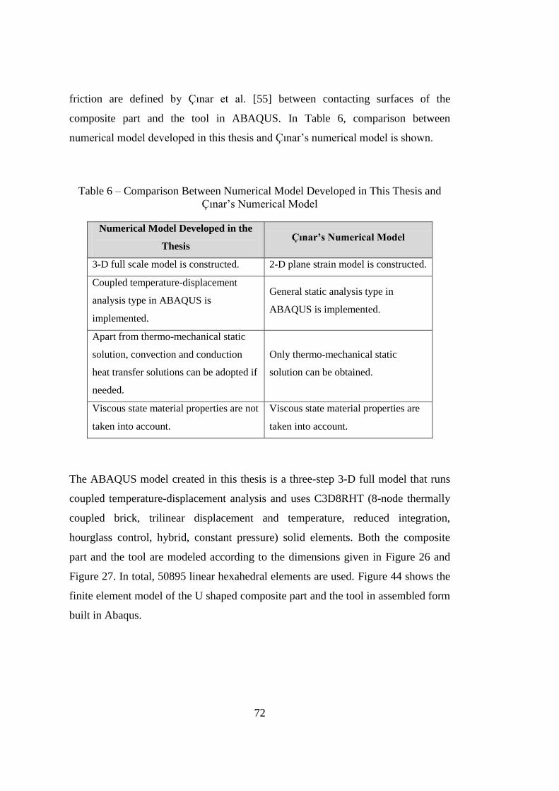
72
friction are defined by Çınar et al. [55] between contacting surfaces of the
composite part and the tool in ABAQUS. In Table 6, comparison between
numerical model developed in this thesis and Çınar’s numerical model is shown.
Table 6 – Comparison Between Numerical Model Developed in This Thesis and
Çınar’s Numerical Model
Numerical Model Developed in the
Thesis Çınar’s Numerical Model
3-D full scale model is constructed. 2-D plane strain model is constructed.
Coupled temperature-displacement
analysis type in ABAQUS is
implemented.
General static analysis type in
ABAQUS is implemented.
Apart from thermo-mechanical static
solution, convection and conduction
heat transfer solutions can be adopted if
needed.
Only thermo-mechanical static
solution can be obtained.
Viscous state material properties are not
taken into account.
Viscous state material properties are
taken into account.
The ABAQUS model created in this thesis is a three-step 3-D full model that runs
coupled temperature-displacement analysis and uses C3D8RHT (8-node thermally
coupled brick, trilinear displacement and temperature, reduced integration,
hourglass control, hybrid, constant pressure) solid elements. Both the composite
part and the tool are modeled according to the dimensions given in Figure 26 and
Figure 27. In total, 50895 linear hexahedral elements are used. Figure 44 shows the
finite element model of the U shaped composite part and the tool in assembled form
built in Abaqus.
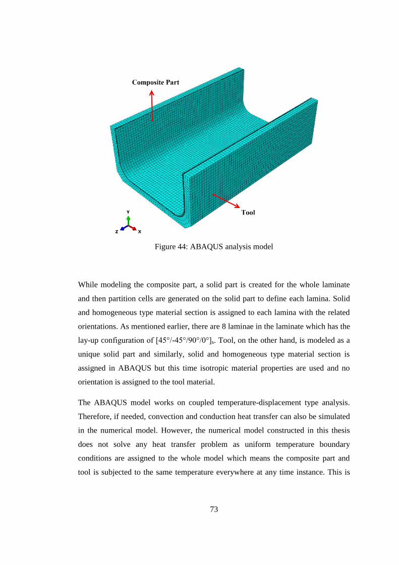
73
Figure 44: ABAQUS analysis model
While modeling the composite part, a solid part is created for the whole laminate
and then partition cells are generated on the solid part to define each lamina. Solid
and homogeneous type material section is assigned to each lamina with the related
orientations. As mentioned earlier, there are 8 laminae in the laminate which has the
lay-up configuration of [45°/-45°/90°/0°]s. Tool, on the other hand, is modeled as a
unique solid part and similarly, solid and homogeneous type material section is
assigned in ABAQUS but this time isotropic material properties are used and no
orientation is assigned to the tool material.
The ABAQUS model works on coupled temperature-displacement type analysis.
Therefore, if needed, convection and conduction heat transfer can also be simulated
in the numerical model. However, the numerical model constructed in this thesis
does not solve any heat transfer problem as uniform temperature boundary
conditions are assigned to the whole model which means the composite part and
tool is subjected to the same temperature everywhere at any time instance. This is

74
because the surface temperature data obtained from experiment by monitoring the
composite part and the tool surfaces at different locations revealed that maximum
temperature gradient among all thermocouple measurements is within the range of
2 . (Figure 33) Therefore, variation in the surface temperature fields for composite
part and tool can be neglected and uniform temperature boundary conditions can be
assigned. On the other hand, for thicker and larger composite parts where
temperature field on the surface differs greatly, the present numerical model can be
modified to take convection heat transfer mechanism into account. The convection
coefficient of autoclave chamber can be determined experimentally and
implemented in the model but this would require additional work. It should be noted
that although the analysis model does not solve any heat transfer problem,
ABAQUS requires a thermal conduction to be defined between contacting surfaces
of the composite part and the tool.
The ABAQUS analysis model considers rubbery and glassy state properties of
composite material and it consists of three steps as mentioned earlier. The first two
steps are illustrated on the cure diagram of AS4/8552 composite system in Figure
45. In the third step, demolding process of the composite part from the tool is
simulated.
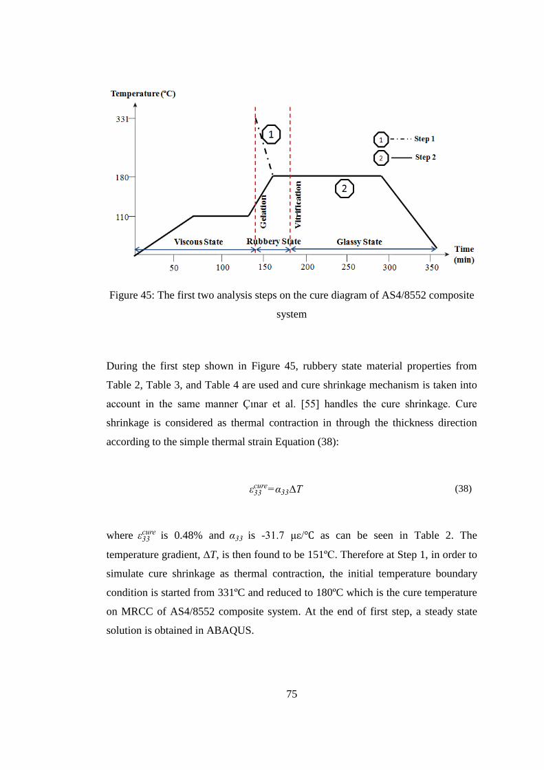
75
Figure 45: The first two analysis steps on the cure diagram of AS4/8552 composite
system
During the first step shown in Figure 45, rubbery state material properties from
Table 2, Table 3, and Table 4 are used and cure shrinkage mechanism is taken into
account in the same manner Çınar et al. [55] handles the cure shrinkage. Cure
shrinkage is considered as thermal contraction in through the thickness direction
according to the simple thermal strain Equation (38):
c T (38)
where c is 0.48% and is -31.7 μ / as can be seen in Table 2. The
temperature gradient, T, is then found to be 151ºC. Therefore at Step 1, in order to
simulate cure shrinkage as thermal contraction, the initial temperature boundary
condition is started from 331ºC and reduced to 180ºC which is the cure temperature
on MRCC of AS4/8552 composite system. At the end of first step, a steady state
solution is obtained in ABAQUS.
76
At Step 2, cooling down from cure temperature to room temperature is simulated.
Therefore, the temperature boundary condition is brought to 25ºC in 2700 seconds.
For a more realistic simulation, transient solution technique is preferred at this step.
During the first and second steps, displacement of four nodes at the corners of
bottom surface of the tool is fixed in x, y, and z directions but no constraint is
applied for the rotation boundary conditions. Figure 46 shows the displacement
boundary condition applied to the corner nodes of the bottom surface of the tool.
Figure 46: Displacement boundary condition applied to the corner nodes of the
bottom surface of the tool
A pressure load of 0.78 MPa representing the combined autoclave chamber pressure
and vacuum pressure is applied to the whole manufacturing assembly during the
first and second steps as shown in Figure 47. At the third step, the pressure load is
removed.
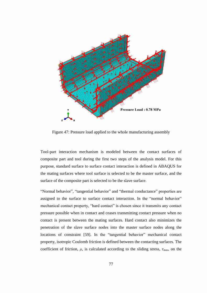
77
Figure 47: Pressure load applied to the whole manufacturing assembly
Tool-part interaction mechanism is modeled between the contact surfaces of
composite part and tool during the first two steps of the analysis model. For this
purpose, standard surface to surface contact interaction is defined in ABAQUS for
the mating surfaces where tool surface is selected to be the master surface, and the
surface of the composite part is selected to be the slave surface.
“Normal behavior”, “tangential behavior” and “thermal conductance” properties are
assigned to the surface to surface contact interaction. In the “normal behavior”
mechanical contact property, “hard contact” is chosen since it transmits any contact
pressure possible when in contact and ceases transmitting contact pressure when no
contact is present between the mating surfaces. Hard contact also minimizes the
penetration of the slave surface nodes into the master surface nodes along the
locations of constraint [59]. In the “tangential behavior” mechanical contact
property, isotropic Coulomb friction is defined between the contacting surfaces. The
coefficient of friction, μ, is calculated according to the sliding stress, τmax, on the
78
contacting surfaces which is accepted to be 0.2 MPa in Step 1 and Step 2 [55].
Equation (39) is used for determining μ:
μ τma
(39)
where P represents the total pressure applied on the manufacturing assembly during
cure and as mentioned earlier, it is 0.78 MPa. The coefficient of friction, μ, is then
found to be 0.26. For the “thermal conductance” thermal contact property, a perfect
thermal conductance which uses clearance-dependency is defined between the
mating surfaces. In reality, engineering surfaces are not completely smooth and
there always exists a surface roughness. These surface irregularities result in
reduced heat transfer between contacting surfaces and conduction heat transfer is
possible through the solid to solid contact points and through the interfacial gaps
[69]. There are available studies in the literature in which thermal conductance
models are presented [70, 71]. However, for the ease of calculation, in the present
study, perfect thermal conductance between composite part and tool is assumed in
the numerical model. To provide perfect thermal conduction meaning there is no
thermal resistance between the contacting surfaces, thermal contact conductance
(TCC) is selected to be a large number in the heat transfer analysis. Thermal
contact conductance is determined in terms of the highest material conductivity
(HMC) used in the model and the diagonal of the overall geometry bounding box
(DOGBB) according to Equation (40) [66]:
TCC = (10000 x HMC) / DOGBB (40)
DOGBB is calculated by measuring the distance between the furthest two points on
tool geometry. TCC is found to be 7.7x10⁶ W/mK which is then approximated as
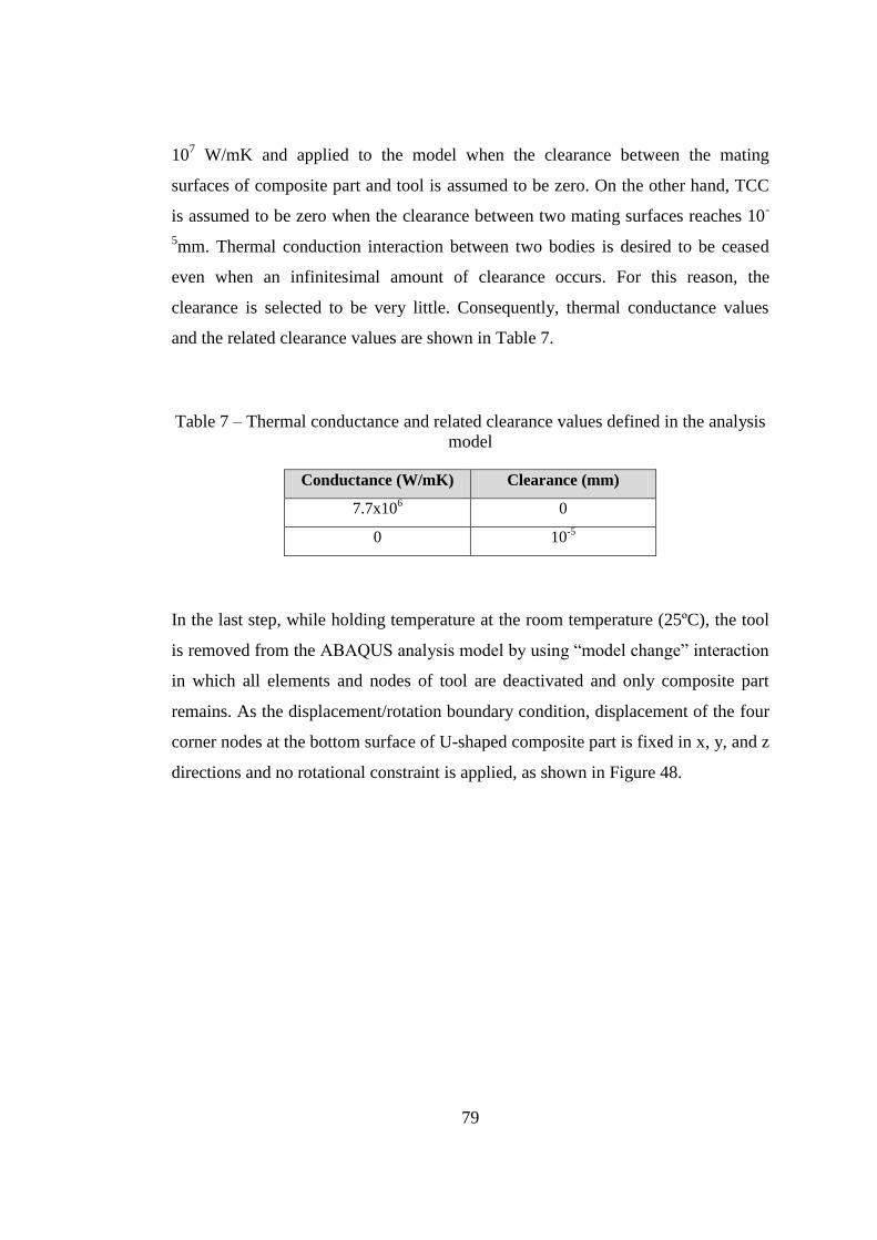
79
107 W/mK and applied to the model when the clearance between the mating
surfaces of composite part and tool is assumed to be zero. On the other hand, TCC
is assumed to be zero when the clearance between two mating surfaces reaches 10-
5mm. Thermal conduction interaction between two bodies is desired to be ceased
even when an infinitesimal amount of clearance occurs. For this reason, the
clearance is selected to be very little. Consequently, thermal conductance values
and the related clearance values are shown in Table 7.
Table 7 – Thermal conductance and related clearance values defined in the analysis
model
Conductance (W/mK) Clearance (mm)
7.7x10⁶ 0
0 10-5
In the last step, while holding temperature at the room temperature (25ºC), the tool
is removed from the ABAQUS analysis model by using “model change” interaction
in which all elements and nodes of tool are deactivated and only composite part
remains. As the displacement/rotation boundary condition, displacement of the four
corner nodes at the bottom surface of U-shaped composite part is fixed in x, y, and z
directions and no rotational constraint is applied, as shown in Figure 48.
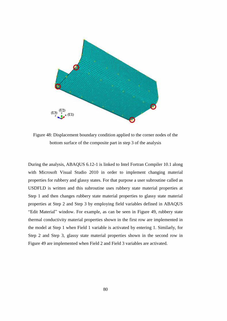
80
Figure 48: Displacement boundary condition applied to the corner nodes of the
bottom surface of the composite part in step 3 of the analysis
During the analysis, ABAQUS 6.12-1 is linked to Intel Fortran Compiler 10.1 along
with Microsoft Visual Studio 2010 in order to implement changing material
properties for rubbery and glassy states. For that purpose a user subroutine called as
USDFLD is written and this subroutine uses rubbery state material properties at
Step 1 and then changes rubbery state material properties to glassy state material
properties at Step 2 and Step 3 by employing field variables defined in ABAQUS
“Edit Material” window. For example, as can be seen in Figure 49, rubbery state
thermal conductivity material properties shown in the first row are implemented in
the model at Step 1 when Field 1 variable is activated by entering 1. Similarly, for
Step 2 and Step 3, glassy state material properties shown in the second row in
Figure 49 are implemented when Field 2 and Field 3 variables are activated.
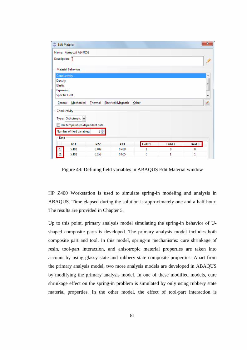
81
Figure 49: Defining field variables in ABAQUS Edit Material window
HP Z400 Workstation is used to simulate spring-in modeling and analysis in
ABAQUS. Time elapsed during the solution is approximately one and a half hour.
The results are provided in Chapter 5.
Up to this point, primary analysis model simulating the spring-in behavior of U-
shaped composite parts is developed. The primary analysis model includes both
composite part and tool. In this model, spring-in mechanisms: cure shrinkage of
resin, tool-part interaction, and anisotropic material properties are taken into
account by using glassy state and rubbery state composite properties. Apart from
the primary analysis model, two more analysis models are developed in ABAQUS
by modifying the primary analysis model. In one of these modified models, cure
shrinkage effect on the spring-in problem is simulated by only using rubbery state
material properties. In the other model, the effect of tool-part interaction is
82
investigated by removing tool from the analysis model. Both modified models are
explained in the following sections.
4.2.3. The Effect of Cure Shrinkage on the Spring-in
In order to understand the effect of cure shrinkage, ABAQUS analysis model is
modified in such a way that only rubbery state material properties are used. The
purpose is to see the spring-in behavior of U-shaped composite part when only cure
shrinkage and tool-part interaction mechanisms are taken into account. Therefore,
the cooling down from the cure temperature to room temperature is not simulated in
this model. The analysis consists of two steps. The previously described modeling
strategy is employed during both steps. In the first step, which is shown in Figure
45 as Step 1, rubbery state material properties are used and cure shrinkage
mechanism is modeled as thermal contraction. Therefore, the temperature of both
composite part and tool is brought to 180ºC from 331ºC. In the second step, while
holding the temperature constant at 180ºC as if the room temperature is reached,
tool is removed from the analysis model and demolding process is simulated. The
results are provided in Chapter 5.
4.2.4. The Effect of Tool-part Interaction on Spring-in
Tool-part interaction has an important effect on the spring-in mechanism. To see
this effect, ABAQUS analysis model is modified such that tool is removed from the
analysis model and surface to surface contact definition between the composite part
and the tool is eliminated. The analysis model only considers composite part and it
consists of two steps which are shown in Figure 45 as Step 1 and Step 2. The
previously described modeling strategy is employed during both steps. In the first
step, rubbery state material properties are used and cure shrinkage mechanism is
modeled as thermal contraction. In the second step, cooling down from cure
temperature to room temperature is simulated by using glassy state material

83
properties. The same boundary conditions and loads are applied to the composite
part. The results are provided in Chapter 5.

84
85
CHAPTER 5
RESULTS AND DISCUSSIONS
In this thesis, spring-in problem of corner shaped composite parts which are made
of AS4/8552 UD prepregs is investigated by three different methods. In the first
method, spring-in problem is solved by employing an analytical model which is
available in the literature. In the analytical model, a 2-D solution is obtained and the
effect of two spring-in mechanisms, cure shrinkage and anisotropy in CTEs, is
taken into account. In the second method, four composite parts are manufactured
with autoclave forming process. During manufacturing process, the surface
temperature of one of the composite parts and its tool is monitored at different
locations to see the variation in temperature. Then, spring-in angles of the
remaining composite parts are measured by using the optical scanning device. In the
third method, a 3-D ABAQUS analysis model which considers the effective spring-
in mechanisms cure shrinkage, anisotropic material properties, and tool-part
interaction is developed. To have a realistic analysis model, changing material
properties are implemented in the analysis model during the cure cycle for the
composite parts. For that purpose, constant rubbery and glassy state material
properties of the composite material available in the literature are used.
Furthermore, effects of cure shrinkage and tool-part interaction mechanisms are
studied separately by modifying the analysis model. In order to see the effect of
cure shrinkage on the spring-in shape distortion, only cure shrinkage mechanism is
simulated. To understand the effect of tool-part interaction, tool is removed from
the analysis model and autoclave forming process is simulated in ABAQUS only
for the composite part.
.
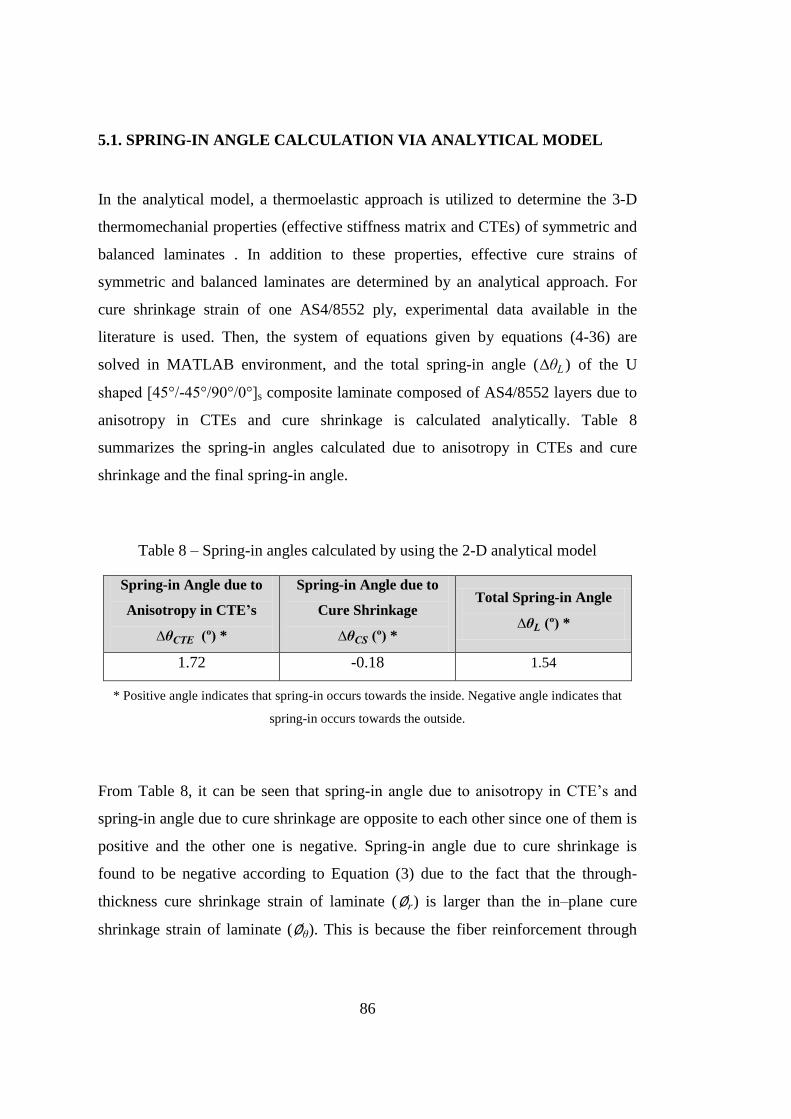
86
5.1. SPRING-IN ANGLE CALCULATION VIA ANALYTICAL MODEL
In the analytical model, a thermoelastic approach is utilized to determine the 3-D
thermomechanial properties (effective stiffness matrix and CTEs) of symmetric and
balanced laminates . In addition to these properties, effective cure strains of
symmetric and balanced laminates are determined by an analytical approach. For
cure shrinkage strain of one AS4/8552 ply, experimental data available in the
literature is used. Then, the system of equations given by equations (4-36) are
solved in MATLAB environment, and the total spring-in angle ( ) of the U
shaped [45°/-45°/90°/0°]s composite laminate composed of AS4/8552 layers due to
anisotropy in CTEs and cure shrinkage is calculated analytically. Table 8
summarizes the spring-in angles calculated due to anisotropy in CTEs and cure
shrinkage and the final spring-in angle.
Table 8 – Spring-in angles calculated by using the 2-D analytical model
Spring-in Angle due to
Anisotropy in CTE’s
(º) *
Spring-in Angle due to
Cure Shrinkage
(º) *
Total Spring-in Angle
(º) *
1.72 -0.18 1.54
* Positive angle indicates that spring-in occurs towards the inside. Negative angle indicates that
spring-in occurs towards the outside.
From Table 8, it can be seen that spring-in angle due to anisotropy in CTE’s and
spring-in angle due to cure shrinkage are opposite to each other since one of them is
positive and the other one is negative. Spring-in angle due to cure shrinkage is
found to be negative according to Equation (3) due to the fact that the through-
thickness cure shrinkage strain of laminate ( ) is larger than the in–plane cure
shrinkage strain of laminate ( ). This is because the fiber reinforcement through
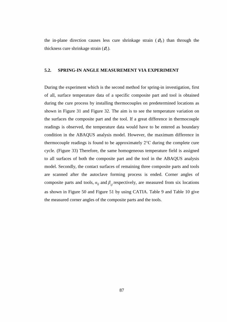
87
the in-plane direction causes less cure shrinkage strain ( ) than through the
thickness cure shrinkage strain ( ).
5.2. SPRING-IN ANGLE MEASUREMENT VIA EXPERIMENT
During the experiment which is the second method for spring-in investigation, first
of all, surface temperature data of a specific composite part and tool is obtained
during the cure process by installing thermocouples on predetermined locations as
shown in Figure 31 and Figure 32. The aim is to see the temperature variation on
the surfaces the composite part and the tool. If a great difference in thermocouple
readings is observed, the temperature data would have to be entered as boundary
condition in the ABAQUS analysis model. However, the maximum difference in
thermocouple readings is found to be approximately 2°C during the complete cure
cycle. (Figure 33) Therefore, the same homogeneous temperature field is assigned
to all surfaces of both the composite part and the tool in the ABAQUS analysis
model. Secondly, the contact surfaces of remaining three composite parts and tools
are scanned after the autoclave forming process is ended. Corner angles of
composite parts and tools, i and i respectively, are measured from six locations
as shown in Figure 50 and Figure 51 by using CATIA. Table 9 and Table 10 give
the measured corner angles of the composite parts and the tools.
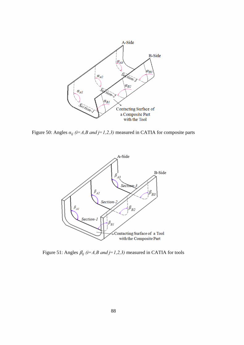
88
Figure 50: Angles i i an measured in CATIA for composite parts
Figure 51: Angles i i an measured in CATIA for tools
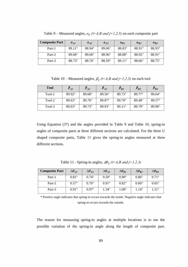
89
Table 9 – Measured angles, i i an on each composite part
Composite Part
Part-1 89.11° 88.94° 89.06° 88.83° 88.91° 88.93°
Part-2 89.06° 89.06° 88.96° 88.88° 88.92° 88.91°
Part-3 88.73° 88.76° 88.59° 89.11° 88.66° 88.75°
Table 10 – Measured angles, i i an on each tool
Tool
Tool-1 89.92° 89.68° 89.56° 89.73° 89.77° 89.64°
Tool-2 89.63° 89.76° 89.87° 89.70° 89.48° 89.57°
Tool-3 89.63° 89.73° 89.93° 90.11° 89.79° 89.96°
Using Equation (37) and the angles provided in Table 9 and Table 10, spring-in
angles of composite parts at three different sections are calculated. For the three U
shaped composite parts, Table 11 gives the spring-in angles measured at three
different sections.
Table 11 - Spring-in angles, i i an
Composite Part
Part-1 0.81° 0.74° 0.50° 0.90° 0.86° 0.71°
Part-2 0.57° 0.70° 0.91° 0.82° 0.60° 0.65°
Part-3 0.91° 0.97° 1.34° 1.00° 1.14° 1.21°
* Positive angle indicates that spring-in occurs towards the inside. Negative angle indicates that
spring-in occurs towards the outside.
The reason for measuring spring-in angles at multiple locations is to see the
possible variation of the spring-in angle along the length of composite part.
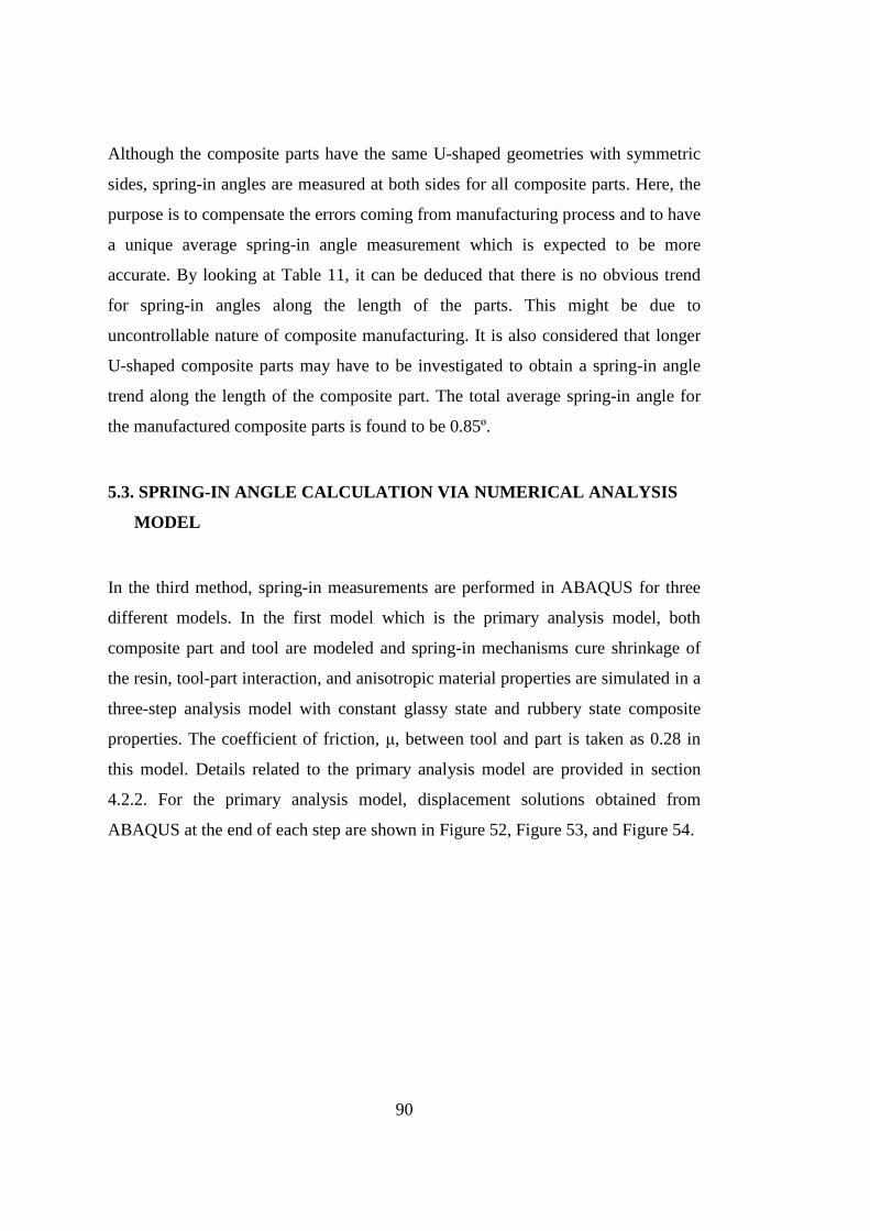
90
Although the composite parts have the same U-shaped geometries with symmetric
sides, spring-in angles are measured at both sides for all composite parts. Here, the
purpose is to compensate the errors coming from manufacturing process and to have
a unique average spring-in angle measurement which is expected to be more
accurate. By looking at Table 11, it can be deduced that there is no obvious trend
for spring-in angles along the length of the parts. This might be due to
uncontrollable nature of composite manufacturing. It is also considered that longer
U-shaped composite parts may have to be investigated to obtain a spring-in angle
trend along the length of the composite part. The total average spring-in angle for
the manufactured composite parts is found to be 0.85º.
5.3. SPRING-IN ANGLE CALCULATION VIA NUMERICAL ANALYSIS
MODEL
In the third method, spring-in measurements are performed in ABAQUS for three
different models. In the first model which is the primary analysis model, both
composite part and tool are modeled and spring-in mechanisms cure shrinkage of
the resin, tool-part interaction, and anisotropic material properties are simulated in a
three-step analysis model with constant glassy state and rubbery state composite
properties. The coefficient of friction, μ, between tool and part is taken as 0.28 in
this model. Details related to the primary analysis model are provided in section
4.2.2. For the primary analysis model, displacement solutions obtained from
ABAQUS at the end of each step are shown in Figure 52, Figure 53, and Figure 54.
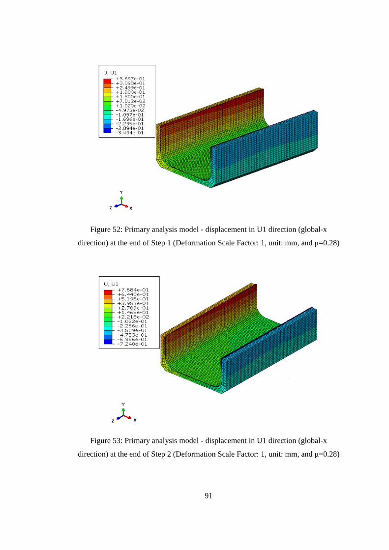
91
Figure 52: Primary analysis model - displacement in U1 direction (global-x
direction) at the end of Step 1 (Deformation Scale Factor: 1, unit: mm, and μ=0.28)
Figure 53: Primary analysis model - displacement in U1 direction (global-x
direction) at the end of Step 2 (Deformation Scale Factor: 1, unit: mm, and μ=0.28)
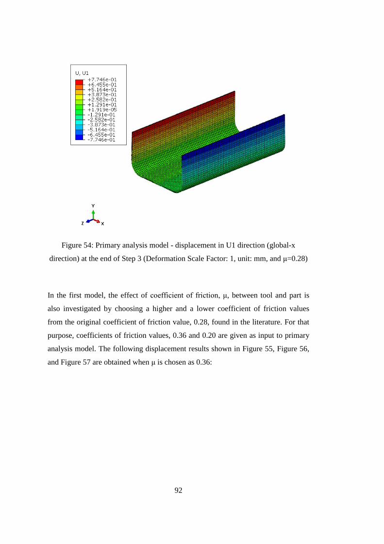
92
Figure 54: Primary analysis model - displacement in U1 direction (global-x
direction) at the end of Step 3 (Deformation Scale Factor: 1, unit: mm, and μ=0.28)
In the first model, the effect of coefficient of friction, μ, between tool and part is
also investigated by choosing a higher and a lower coefficient of friction values
from the original coefficient of friction value, 0.28, found in the literature. For that
purpose, coefficients of friction values, 0.36 and 0.20 are given as input to primary
analysis model. The following displacement results shown in Figure 55, Figure 56,
and Figure 57 are obtained when μ is chosen as 0.36:
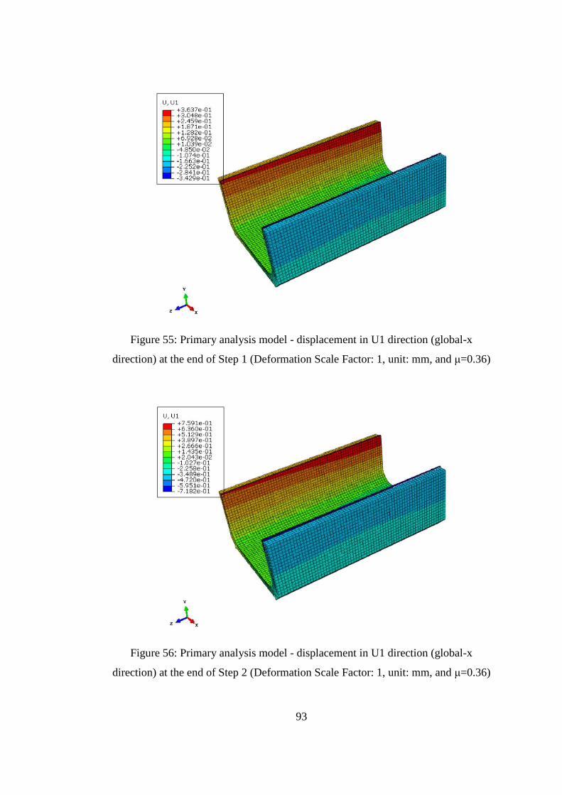
93
Figure 55: Primary analysis model - displacement in U1 direction (global-x
direction) at the end of Step 1 (Deformation Scale Factor: 1, unit: mm, and μ=0.36)
Figure 56: Primary analysis model - displacement in U1 direction (global-x
direction) at the end of Step 2 (Deformation Scale Factor: 1, unit: mm, and μ=0.36)
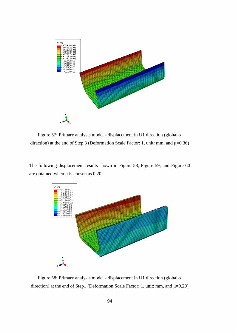
94
Figure 57: Primary analysis model - displacement in U1 direction (global-x
direction) at the end of Step 3 (Deformation Scale Factor: 1, unit: mm, and μ=0.36)
The following displacement results shown in Figure 58, Figure 59, and Figure 60
are obtained when μ is chosen as 0.20:
Figure 58: Primary analysis model - displacement in U1 direction (global-x
direction) at the end of Step1 (Deformation Scale Factor: 1, unit: mm, and μ=0.20)
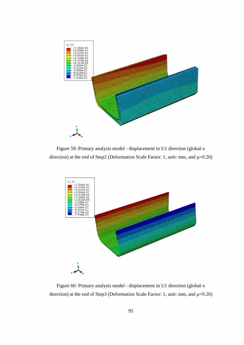
95
Figure 59: Primary analysis model - displacement in U1 direction (global-x
direction) at the end of Step2 (Deformation Scale Factor: 1, unit: mm, and μ=0.20)
Figure 60: Primary analysis model - displacement in U1 direction (global-x
direction) at the end of Step3 (Deformation Scale Factor: 1, unit: mm, and μ=0.20)
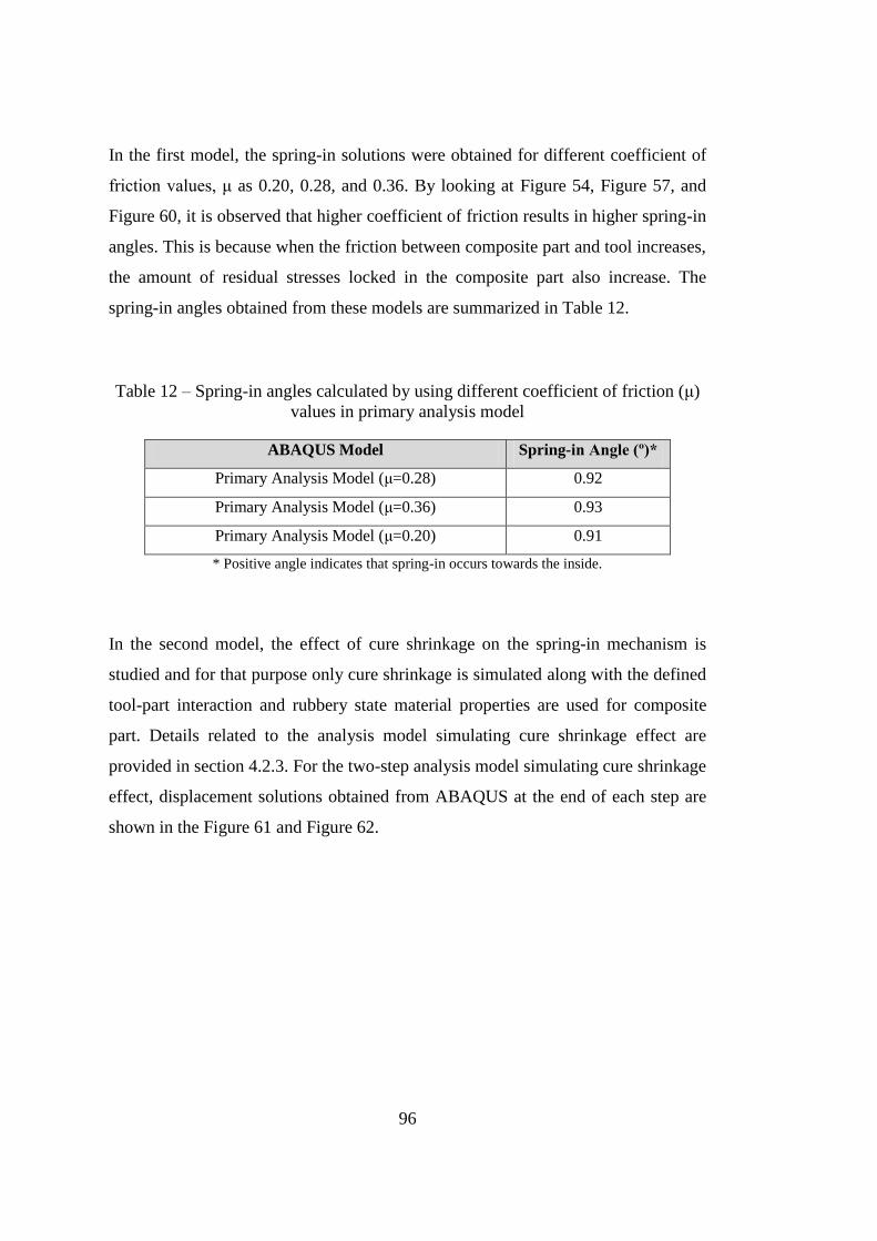
96
In the first model, the spring-in solutions were obtained for different coefficient of
friction values, μ as 0.20, 0.28, and 0.36. By looking at Figure 54, Figure 57, and
Figure 60, it is observed that higher coefficient of friction results in higher spring-in
angles. This is because when the friction between composite part and tool increases,
the amount of residual stresses locked in the composite part also increase. The
spring-in angles obtained from these models are summarized in Table 12.
Table 12 – Spring-in angles calculated by using different coefficient of friction (μ)
values in primary analysis model
ABAQUS Model Spring-in Angle (º)*
Primary Analysis Model (μ=0.28) 0.92
Primary Analysis Model (μ=0.36) 0.93
Primary Analysis Model (μ=0.20) 0.91
* Positive angle indicates that spring-in occurs towards the inside.
In the second model, the effect of cure shrinkage on the spring-in mechanism is
studied and for that purpose only cure shrinkage is simulated along with the defined
tool-part interaction and rubbery state material properties are used for composite
part. Details related to the analysis model simulating cure shrinkage effect are
provided in section 4.2.3. For the two-step analysis model simulating cure shrinkage
effect, displacement solutions obtained from ABAQUS at the end of each step are
shown in the Figure 61 and Figure 62.
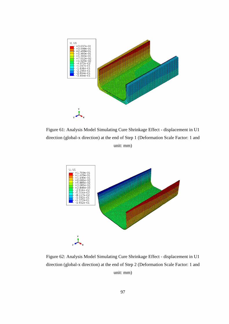
97
Figure 61: Analysis Model Simulating Cure Shrinkage Effect - displacement in U1
direction (global-x direction) at the end of Step 1 (Deformation Scale Factor: 1 and
unit: mm)
Figure 62: Analysis Model Simulating Cure Shrinkage Effect - displacement in U1
direction (global-x direction) at the end of Step 2 (Deformation Scale Factor: 1 and
unit: mm)
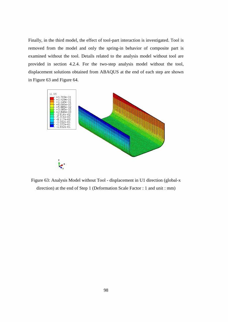
98
Finally, in the third model, the effect of tool-part interaction is investigated. Tool is
removed from the model and only the spring-in behavior of composite part is
examined without the tool. Details related to the analysis model without tool are
provided in section 4.2.4. For the two-step analysis model without the tool,
displacement solutions obtained from ABAQUS at the end of each step are shown
in Figure 63 and Figure 64.
Figure 63: Analysis Model without Tool - displacement in U1 direction (global-x
direction) at the end of Step 1 (Deformation Scale Factor : 1 and unit : mm)
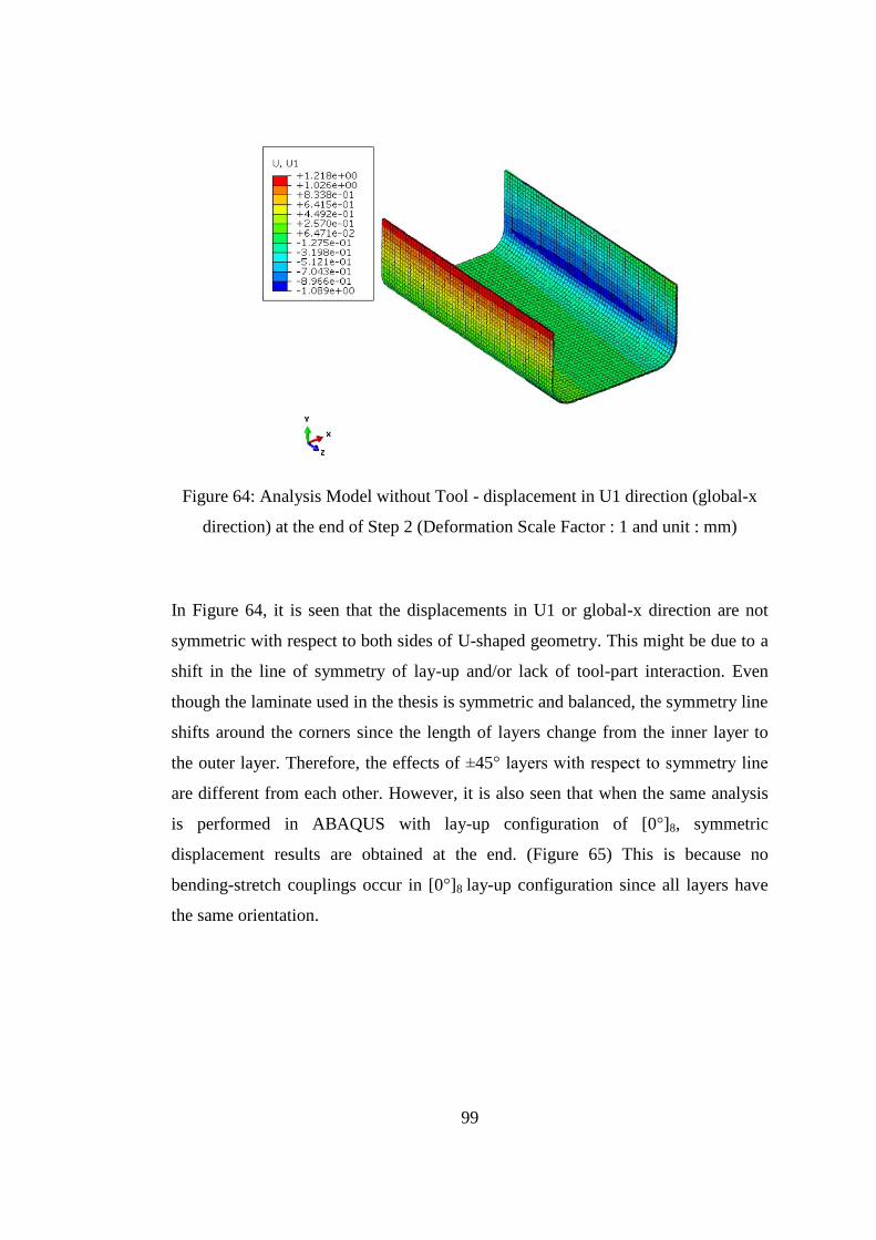
99
Figure 64: Analysis Model without Tool - displacement in U1 direction (global-x
direction) at the end of Step 2 (Deformation Scale Factor : 1 and unit : mm)
In Figure 64, it is seen that the displacements in U1 or global-x direction are not
symmetric with respect to both sides of U-shaped geometry. This might be due to a
shift in the line of symmetry of lay-up and/or lack of tool-part interaction. Even
though the laminate used in the thesis is symmetric and balanced, the symmetry line
shifts around the corners since the length of layers change from the inner layer to
the outer layer. Therefore, the effects of ±45° layers with respect to symmetry line
are different from each other. However, it is also seen that when the same analysis
is performed in ABAQUS with lay-up configuration of [0°]8, symmetric
displacement results are obtained at the end. (Figure 65) This is because no
bending-stretch couplings occur in [0°]8 lay-up configuration since all layers have
the same orientation.
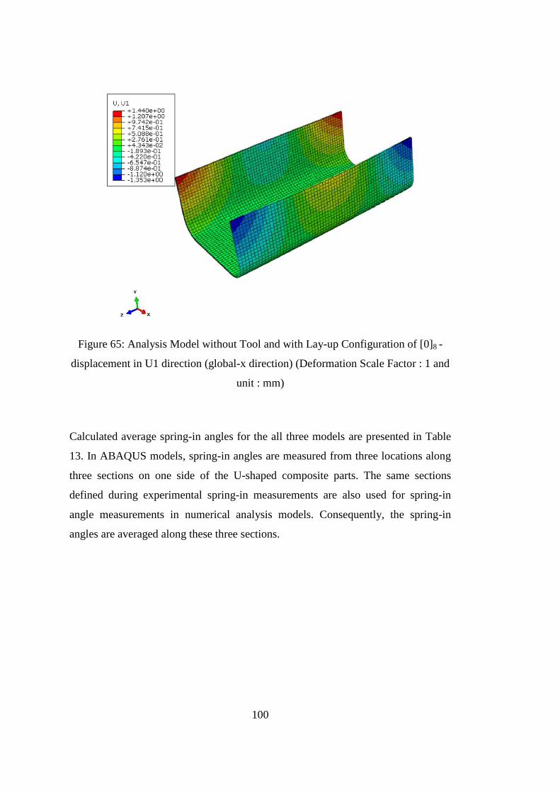
100
Figure 65: Analysis Model without Tool and with Lay-up Configuration of [0]8 -
displacement in U1 direction (global-x direction) (Deformation Scale Factor : 1 and
unit : mm)
Calculated average spring-in angles for the all three models are presented in Table
13. In ABAQUS models, spring-in angles are measured from three locations along
three sections on one side of the U-shaped composite parts. The same sections
defined during experimental spring-in measurements are also used for spring-in
angle measurements in numerical analysis models. Consequently, the spring-in
angles are averaged along these three sections.
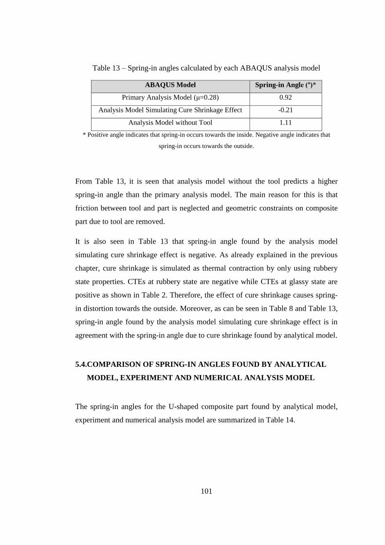
101
Table 13 – Spring-in angles calculated by each ABAQUS analysis model
ABAQUS Model Spring-in Angle (º)*
Primary Analysis Model (μ=0.28) 0.92
Analysis Model Simulating Cure Shrinkage Effect -0.21
Analysis Model without Tool 1.11
* Positive angle indicates that spring-in occurs towards the inside. Negative angle indicates that
spring-in occurs towards the outside.
From Table 13, it is seen that analysis model without the tool predicts a higher
spring-in angle than the primary analysis model. The main reason for this is that
friction between tool and part is neglected and geometric constraints on composite
part due to tool are removed.
It is also seen in Table 13 that spring-in angle found by the analysis model
simulating cure shrinkage effect is negative. As already explained in the previous
chapter, cure shrinkage is simulated as thermal contraction by only using rubbery
state properties. CTEs at rubbery state are negative while CTEs at glassy state are
positive as shown in Table 2. Therefore, the effect of cure shrinkage causes spring-
in distortion towards the outside. Moreover, as can be seen in Table 8 and Table 13,
spring-in angle found by the analysis model simulating cure shrinkage effect is in
agreement with the spring-in angle due to cure shrinkage found by analytical model.
5.4.COMPARISON OF SPRING-IN ANGLES FOUND BY ANALYTICAL
MODEL, EXPERIMENT AND NUMERICAL ANALYSIS MODEL
The spring-in angles for the U-shaped composite part found by analytical model,
experiment and numerical analysis model are summarized in Table 14.
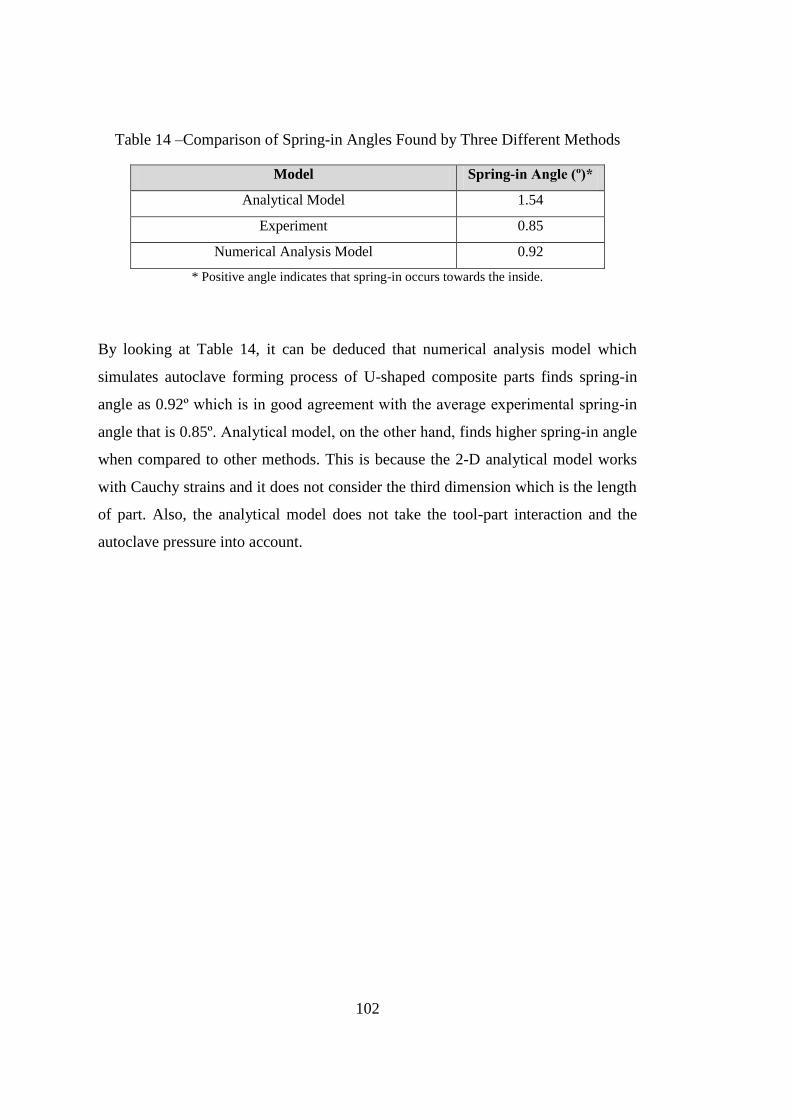
102
Table 14 –Comparison of Spring-in Angles Found by Three Different Methods
Model Spring-in Angle (º)*
Analytical Model 1.54
Experiment 0.85
Numerical Analysis Model 0.92
* Positive angle indicates that spring-in occurs towards the inside.
By looking at Table 14, it can be deduced that numerical analysis model which
simulates autoclave forming process of U-shaped composite parts finds spring-in
angle as 0.92º which is in good agreement with the average experimental spring-in
angle that is 0.85º. Analytical model, on the other hand, finds higher spring-in angle
when compared to other methods. This is because the 2-D analytical model works
with Cauchy strains and it does not consider the third dimension which is the length
of part. Also, the analytical model does not take the tool-part interaction and the
autoclave pressure into account.
103
CHAPTER 6
CONCLUSIONS
In this thesis, spring-in problem encountered in U-shaped composite parts which are
made of Hexcel’s AS4/8552 unidirectional (UD) prepregs with lay-up configuration
[45°/-45°/90°/0°]s is investigated by analytical, experimental and numerical
methods. First of all, a simple two dimensional (2-D) geometrical model available
in the literature is implemented and spring-in is calculated according to this model.
Secondly, using autoclave forming technique, U-shaped composite parts are
manufactured and spring-in measurements are performed on these parts by using
optical scanning device. Finally, a three dimensional (3-D) numerical model in
ABAQUS is constructed by taking tool-part interaction, cure shrinkage and state
transformations of resin into account. Then spring-in simulation is performed by
using constant rubbery and glassy state material properties for U-shaped composite
parts.
Spring-in angle 1.54º calculated with analytical method is observed to be higher
than spring-in angles determined by the numerical and the experimental methods.
Therefore, it is concluded that although 2-D analytical model is a fast method to
predict spring-in behavior of a corner shaped composite part, it overestimates the
spring-in angle.
It can be deduced from the overestimated results of analytical model that tool-part
interaction is an important spring-in mechanism which must be taken into account
for proper spring-in estimation. The importance of tool-part interaction mechanism
is also seen in the numerical analyses. The numerical analysis performed without
the tool gave spring-in angle of 1.11º which is higher than the spring angle of 0.92º
found by primary analysis model which includes tool model and, therefore; tool-
part interaction.

104
The effect of cure shrinkage causes a spring-in behavior towards the outside for a
U-shaped composite part. This is validated by both analytical and numerical results.
Negative spring-in angles of -0.18º and -0.21º are obtained from the analytical and
numerical models, respectively. Negative spring-in angles mean that the spring-in
occurs towards the outside. It can be stated that analytical model and numerical
model make a good agreement while calculating spring-in angle due to cure
shrinkage mechanism.
As mentioned earlier, spring-in angle 0.92º found by primary analysis model which
is the basic numerical model developed in ABAQUS is very close to the average
spring-in angle 0.85º obtained via experiment. Therefore, ABAQUS analysis model
is found to be satisfactory since it yields acceptable spring-in angle prediction with
respect to the real case spring-in angle measured during experiment. It is concluded
that the ABAQUS analysis model can be used to predict the spring-in angle of a
composite part so that more accurate tools can be manufactured beforehand. This
reduces manufacturing costs and time.
For future studies, in order to have a more realistic numerical analysis model, heat
transfer inside the autoclave chamber can be modeled. For that purpose, convection
coefficient should be experimentally determined and implemented in the analysis
model. Also, to see the variation of spring-in along the length of U-shaped
composite parts, experiments and numerical analyses with longer composite parts
should be conducted. In addition to these, spring-in behavior of a different type of
reinforcement such as woven fabric reinforcement can be studied in the numerical
analysis and experiments. Plane stress and strain models of the composite parts can
be developed to make comparisons against the 2D analytical prediction presented in
this thesis.
105
REFERENCES
[1] Harris, B., (1999). Engineering Composite Materials. London: The Institute of
Materials.
[2] Mohan, M., (2008). The Advantages of Composite Materials in Marine
Renewable Energy Structures. Paper presented at RINA Marine Renewable Energy
Conference. pp.1-3
[3] Biron, M., (2014). Thermosets and Composites. 2nd ed. San Diego, USA:
Elsevier.
[4] Ratna, D., (2009). Handbook of Thermoset Resins. 1st ed. UK: Smithers.
[5] Lamers, E. A. D., (2004). Shape distortions in fabric reinforced composite
products due to processing induced fibre reorientation. 1st ed. The Netherlands:
FEBO druk, Enschede.
[6] Ibeh, C.C., (2011). Thermoplastic Materials: Properties, Manufacturing
Methods, and Applications. 1st ed. : CRC Press.
[7] Todd Johnson (2008). Thermoplastic vs Thermoset Resins. [ONLINE]
Available at:
http://composite.about.com/od/aboutcompositesplastics/a/Thermoplastic-Vs-
Thermoset-Resins.htm. [Last Accessed 13 July 2014].
[8] Henning, F., Krause, W., (2005). Long-Fiber Reinforced Thermoplastics
Tailored for Structural Performance. ACCE, 5th Automotive and Composites
Conference. USA.
[9] Daniel, M.I., Ishai, O., (1994). Engineering Mechanics of Composite Materials.
1st ed. New York: Oxford University Press.
[10] Tong, L., Mouritz, A. P., and Bannister, M. K., (2002). 3D Fiber Reinforced
Polymer Composites. 1st ed. Sydney: Elsevier.
[11] Bilisik, K., (2013). Three-dimensional braiding for composites: A review.
Textile Research Journal. 83 (13), pp.1414-1436
[12] Campbell, F.C., (2003). Manufacturing Processes for Advanced Composites.
Missouri: Elsevier.
[13] Vasiliev, V. V., Morozov, E. V., (2001). Mechanics and Analysis of
Composite Materials. 1st ed. Oxford: Elsevier.
106
[14] Harper, A. C., Petrie, M. E., (2003). Plastics Materials and Processes: A
Concise Encyclopedia. John Wiley & Sons, Inc..
[15] Laurenzi, S. and Marchetti, M. (2012). Advanced Composite Materials by
Resin Transfer Molding for Aerospace Applications, Composites and Their
Properties, Prof. Ning Hu (Ed.), ISBN: 978-953-51-0711-8, InTech, DOI:
10.5772/48172. Available from: http://www.intechopen.com/books/composites-
and-their-properties/advanced-composite-materials-by-resin-transfer-molding-for-
aerospace-applications
[16] Hoa, V. S., (2009). Principles of the Manufacturing of Composite Materials.
1st ed. USA: DEStech Publications.
[17] Hexcel (2005). Prepreg Technology. France: Publication No. FGU 017b.
[18] West System, (2010). Vacuum Bagging Techniques. 7th ed. Bay City:
Gougeon Brothers.
[19] Bersee, H.E.N., Lindstedt, S., Niño, G., Beukers, A., (2007). DIAPHRAGM
FORMING OF THERMOSET COMPOSITES. 16TH INTERNATIONAL
CONFERENCE ON COMPOSITE MATERIALS. pp.1-2
[20] Lavender CE (2010). Guide to Vacuum Bagging. [ONLINE] Available at:
http://www.lavender-ce.com/wp-content/uploads/guide-to-vacuum-bagging.pdf.
[Last Accessed 15.07.2014].
[21] Hexcel, (2013). HexPly 8552 Product Data. 1st ed. France: Hexcel Composites
Publication.
[22] FAA-H-8083-31, (2014). Aviation Maintenance Technician Handbook -
Airframe. 1st ed. USA
[23] Fernlund, G., Poursartip, A., Twigg, G., and Albert, C., (2002). RESIDUAL
STRESS, 2 IN AUTOCLAVED COMPOSITE PARTS. Vancouver: The University
of British Columbia.
[24] Antonucci V., Giordano M., Cusano A., Nasser J., Nicolais L., (2006). Real
time monitoring of cure and gelification of a thermoset matrix. Composites Science
and Technology. 66, pp.3273–3280
[25] ACP Composites (2013). Prepregs. [ONLINE] Available at:
https://www.acpsales.com/upload/what-are-prepregs.pdf. [Last Accessed 16 July
2014].
[26] Leutz, D., (2011). Draping Simulation: Modelling different Materials and
Processes. München: SGL GROUP.
107
[27] PAM-QUIKFORM for CATIA V5 (2007). [ONLINE] Available at:
http://www.plmmarketplace.com/software/pam-quikform-for-catia-v5.html. [Last
Accessed 17 July 2014].
[28] Woytowich, Brian J., (2008). Detection of delamination defects in carbon fiber
laminate composites using ultrasound and the Hilbert-Huang transform.
Massachusetts: Tufts University
[29] P. Camanhoa, P., G. Da´vila, C., Pinhoc, S., Iannucci, L., Robinson, P., (2006).
Prediction of in situ strengths and matrix cracking in composites under transverse
tension and in-plane shear. Composites. 37 (Part A), pp. 165–176
[30] Wisnom, M.R., Gigliotti, M., Ersoy, N., Campbell, M., Potter, K.D. , (2006).
Mechanisms generating residual stresses and distortion during manufacture of
polymer–matrix composite structures. Composites. 37 (Part A), pp.522-529
[31] Twigg, G., Poursartip, A., Fernlund, G., (2004). Tool–part interaction in
composites processing. Part I: experimental investigation and analytical model.
Composites. 35 (Part A), pp.121-133
[32] Albert, C., Fernlund, G., (2002). Spring-in and warpage of angled composite
laminates. Composites Science and Technology. 62 (), pp.1895-1912
[33] Wijskamp, S., (2005). Shape Distortions in Composite Forming. 1st ed. The
Netherlands: PrintPartners Ipskamp B.V.
[34] Salomi, A., Garstka T., Potter K., Greco, A., Maffezzoli, A., (2002). Spring-in
angle as molding distortion for thermoplastic matrix composite. Composites
Science and Technology. 68, pp.3047-3054
[35] Svanberg, J.M., Holmberg, J. A., (2004). Prediction of shape distortions Part I.
FE-implementation of a path dependent constitutive model. Composites. 35 (Part
A), pp.711-721
[36] Svanberg, J.M., (2002). Predictions of manufacturing induced shape
distortions-high performance thermoset composites. Sweden: Department of
Applied Physics and Mechanical Engineering, Lulea University of Technology.
[37] Ersoy, N., Tugutlu, M., (2010). Cure Kinetics Modeling and Cure Shrinkage
Behavior of a Thermosetting Composite. POLYMER ENGINEERING AND
SCIENCE. 50, pp.84-92
[38] Shokrieh, M.M., Safarabadi, M., (2011). Three-dimensional analysis of micro-
residual stresses in fibrous composites based on the energy method: a study
including interphase effects. Journal of Composite Materials. 46 (6), pp.727-735
108
[39] Nawab, Y., Tardif, X., Boyard, N., Sobotka, V., Casari, P., Jacquemin, F.,
(2012). Determination and modelling of the cure shrinkage of epoxy vinylester resin
and associated composites by considering thermal gradients. Composites Science
and Technology. 73, pp.81-87
[40] Hoa, S.V., Ouellette, P., Ngo, T.D., (2009). Determination of Shrinkage and
Modulus Development of Thermosetting Resins. Journal of Composite Materials.
43 (783).
[41] Yoon, K. J., Kim, J-S., (2001). Effect of Thermal Deformation and Chemical
Shrinkage on the Process Induced Distortion of Carbon/Epoxy Curved Laminates.
Journal of Composite Materials. 35 (253).
[42] Russell, J.D., Madhukar, M.S., Genidy, Lee, A.Y., (2000). A New Method to
Reduce Cure-Induced Stresses in Thermoset Polymer Composites, Part III:
Correlating Stress History to Viscosity, Degree of Cure, and Cure Shrinkage.
Journal of Composite Materials. 34 (1926).
[43] Zeng, X., Raghavan, J., (2010). Role of tool-part interaction in process-induced
warpage of autoclave-manufactured composite structures. Composites. 41 (Part A),
pp.1174-1183
[44] Dong, C., (2009). Modeling the Dimensional Variations of Composites Using
Effective Coefficients of Thermal Expansion. Journal of Composite Materials. 43
(2639).
[45] Wisnom, M. R., Potter, K. D., and Ersoy, N., (2007). Shear-lag Analysis of the
Effect of Thickness on Spring-in of Curved Composites. Journal of Composite
Materials. 41 (1311)
[46] Radford, D.W., Rennic, T.S., (2000). Separating sources of manufacturing
distortion in laminated composites. Journal of Reinforeced Plastics Composites. 19
(8), pp.621-641
[47] Chen, H-J. and Tsai, S.W., (1996). Three-Dimensional Effective Moduli of
Symmetric Laminates. Journal of Composite Materials. 30 (906).
[48] Goetschel, D.B., and Radford, D.W., (1997). Analytical development of
through–thickness properties of composite laminates. Journal of Advanced
Materials, 28(4), pp.37–46.
[49] Akkerman, R., (2002). On the properties of quasi–isotropic laminates.
Composites Part B: Engineering, 33, pp.133–140.
[50] Roylance, D., (2001). Transformation of Stresses and Strains, Department of
Materials Science and Engineering, MIT, USA.
109
[51] Ersoy, N., Garstka, T., Potter, K., Wisnom, M.R., Porter, D., Clegg, M.,
Stringer, G., (2010). Development of the properties of a carbon fibre reinforced
thermosetting composite through cure. Composites. 41 (Part A), pp.401-409
[52] HexTow, AS4, (2013). Product Data. France: Hexcel.
[53] HexPly, 8552 Epoxy Matrix, (2013). Product Data. France: Hexcel.
[54] FREKOTE, 700-NC, (2009). Technical Data Sheet. Germany: Henkel
[55] Çinar, K., Öztürk, U. E., Ersoy, N., Wisnom, M.R., (2013) Modeling
manufacturing deformations in corner sections made of composite materials.
Journal of Composite Materials, 0(0) 1–15.
[56] ZAIMOVIC-UZUNOVIC, N., LEMES, S., (2010) Influences Of Surface
Parameters On Laser 3d Scanning, 10th International Symposium on Measurement
and Quality Control.
[57] Khoun, L., Centea, T., Hubert, P., (2009). Characterization Methodology of
Thermoset Resins for the Processing of Composite Materials -- Case Study:
CYCOM 890RTM Epoxy Resin. Journal of Composite Materials. 44 (1397)
[58] Ersoy, N., Garstka, T., Potter, K., Wisnom, M.R., Porter, D., Stringer, G.,
(2009) Modelling of the spring-in phenomenon in curved parts made of a
thermosetting composite. Composites. 41 (Part A), pp.410-418
[59] SIMULIA, ABAQUS 6.12-1. ABAQUS Analysis User's Manual.
[60] Johnston, A.A., (1997). An Integrated Model of the Development of Process-
Induced Deformation in Autoclave Processing of Composite Structures. Canada:
Department of Metals and Materials Engineering, The University of British
Columbia.
[61] Zhu, Q., Geubelle, P.H., (2002). Dimensional Accuracy of Thermoset
Composites: Shape Optimization, Journal of Composite Materials. 36 (647)
[62] Wiersma, H.W., Peeters, L.J.B., Akkerman, R., (1998). Prediction of
springforward in continuous-fibre/polymer L-shaped parts. The Netherlands:
Department of Mechanical Engineering, University of Twente.
[63] Dong, C., Zhang, C., Liang, Z., Wang, B., (2003) Dimension variation
prediction for composites with finite element analysis and regression modeling,
Composites. 35 (Part A), pp.735-746
[64] Fernlund, G., Osooly, A., Poursartip, A., Vaziri, R., Courdji, R., Nelson, K.,
George, P., Hendrickson, L., Griffith, J., (2003). Finite element based prediction of
110
process-induced deformation of autoclaved composite structures using 2D process
analysis and 3D structural analysis, Composite Structures. 62, pp.223-234
[65] Svanberg, J.M., Holmberg, J.A., (2004). Prediction of shape distortions. Part II.
Experimental validation and analysis of boundary conditions, Composites. 35 (Part
A), pp.723-734
[66] Ruiz, M. J. G., (2009). Thermal Analysis in ANSYS. Columbia: Mechanical
Engineering Department, Universidad EAFIT.
[67] Dynamic Mechanical Analysis (DMA), (2013). USA: PerkinElmer Inc.
[68] ASM Aerospace Specification Metals Inc. (2001). [ONLINE] Available at:
http://asm.matweb.com/search/GetReference.asp?bassnum=MA6061t6. [Last
Accessed 25 June 2014].
[69] Misra, P., Nagaraju, J., (2010). Thermal gap conductance at low contact
pressures (<1 MPa): Effect of gold plating and plating thickness, International
Journal of Heat and Mass Transfer. 53, 5373-5379
[70] Milanez, F., Yovanovic, M. M., Mantelli, M.B.H., (2003). Thermal Contact
Conductance At Low Contact Pressures, 36th AIAA Thermophysics Conference,
Orlando, FL
[71] Cooper, M. G., Mikict, B. B., Yovanovich M. M., (1969), Thermal Contact
Conductance. International Journal of Heat and Mass Transfer, 12, pp.279-303