Experimental and Computational Studies on Cryogenic Turboexpander

A Thesis Submitted for Award of the Degree of

Doctor of Philosophy

Subrata Kumar Ghosh

Mechanical Engineering Department

National Institute of Technology Rourkela 769008

Dedicated to

PARENTS

NATIONAL INSTITUTE OF TECHNOLOGY ROURKELA, INDIA

Ranjit Kr Sahoo Sunil Kr Sarangi Professor Director Mechanical Engg. Department NIT Rourkela NIT Rourkela Date: July 29, 2008

This is to certify that the thesis entitled “Experimental and computational studies

on Cryogenic Turboexpander”, being submitted by Shri Subrata Kumar Ghosh, is

a record of bona fide research carried out by him at Mechanical Engineering

department, National Institute of Technology, Rourkela, under our guidance and

supervision. The work incorporated in this thesis has not been, to the best of our

knowledge, submitted to any other university or institute for the award of any

degree or diploma.

(Ranjit Kr Sahoo) (Sunil Kr Sarangi)

CERTIFICATE

iv

Acknowledgement

I am extremely fortunate to be involved in an exciting and challenging research project

like development of a high speed cryogenic turboexpander. It has enriched my life, giving me an

opportunity to look at the horizon of technology with a wide view and to come in contact with

people endowed with many superior qualities.

I would like to express my deep sense of gratitude and respect to my supervisors Prof.

S.K.Sarangi and Prof. R.K.Sahoo for their excellent guidance, suggestions and constructive

criticism. I feel proud that I am one their doctoral students. The charming personality of Prof.

Sarangi has been unified perfectly with knowledge that creates a permanent impression in my

mind. I consider myself extremely lucky to be able to work under the guidance of such a dynamic

personality. Whenever I faced any problem – academic or otherwise, I ran to him, and he was

always there, with his reassuring smile, to bail me out. I and my family members also remember

the affectionate love and kind support extended by Madam Sarangi during our stay at Kharagpur

and Rourkela.

I also feel lucky to get Prof. R.K.Sahoo as one of my supervisors. His invaluable academic

and family support and creative suggestions helped me a lot to complete the project successfully.

I record my deepest gratitude to Madam Sahoo for family support all the times during our stay at

Rourkela.

I take this opportunity to express my heartfelt gratitude to the members of my doctoral

scrutiny committee – Prof. B. K. Nanda (HOD), Prof. A. K. Shatpaty of Mechanical Engineering

Department, Prof. R. K. Singh of Chemical Engineering Department for thoughtful advice and

useful discussions. I am thankful to my other teachers at the Mechanical Engineering Department

for constant encouragement and support in pursuing the PhD work.

I am indebted to the Cryogenic Division of Bhabha Atomic Research Centre (BARC), Mr.

Tilok Singh and his Team for sharing their vast experience on turbine. I must confess – had he

not made arrangements for the experiments of our turbine in BARC, I would not be in a position

to write these words now.

I take this opportunity to express my heartfelt gratitude to all the staff members of

Mechanical Engineering Department, NIT Rourkela for their valuable suggestions and timely

support. I am deeply indebted to one of the project team members Mr. Biswanath Mukherjee for

his cooperation and skilled technical support to complete the task in time. I record my

appreciation for the help extended by Dr. Nagam Seshaiah during my research work.

“A friend in need is a friend indeed” – I have got a first hand proof of this proverb

through the generosity of my friends and associates at NIT. Mr. Pradip Kumar Roy and Mr Suhrit

v

Mula, my good friends have been by my side all my life at NIT. I shall really miss the interesting

and intellectually motivating company of my friends and colleagues.

I am really grateful to my loving parents for their perseverance, encouragement with

support of all kinds and their unconditional affection. With a smile on their faces but anxiety in

their minds, they stood by my side in times of need. Their presence itself came as a soothing

solace. I thank my stars to have such wonderful parents. My beloved wife had to undergo the

rigours of my agony and ecstasy during the period of my research work. Sometimes she had to

manage difficult and demanding situations all alone. I am sorry for this but feel proud of her.

This thesis is a fruit of the fathomless love and affection of all the people around me –

my wife, parents, in-laws, grandparents, uncle and aunty, brother, my supervisors and my

colleagues and friends. If there is anything in this work that is of value – the credit goes entirely

to them.

(July 29, 2008) (Subrata Kumar Ghosh)

vi

Abstract

The expansion turbine constitutes the most critical component of a large number of

cryogenic process plants – air separation units, helium and hydrogen liquefiers, and low

temperature refrigerators. A medium or large cryogenic system needs many components,

compressor, heat exchanger, expansion turbine, instrumentation, vacuum vessel etc. At present

most of these process plants operate at medium or low pressure due to its inherent advantages.

A basic component which is essential for these processes is the turboexpander. The theory of

small turboexpanders and their design method are not fully standardised. Although several

companies around the world manufacture and sell turboexpanders, the technology is not

available in open literature. To address to this problem, a modest attempt has been made at NIT,

Rourkela to understand, standardise and document the design, fabrication and testing procedure

of cryogenic turboexpanders. The research programme has two major objectives –

⇒ A clear understanding of the thermodynamic scenario though modelling, that will help

in determination of blade profile, and prediction of its performance for a given speed

and size.

⇒ To build and record in open literature a complete turbine system.

The work presented here can be broadly classified into seven parts. The first part is the

genesis that builds up the problem and gives a comprehensive review of turboexpander

literature. A detailed review of the development process, as well as all relevant technical issues,

have been carried out and will be presented in the thesis.

A streamlined design procedure, based on published works, has been developed and

documented for all the components. Full details of the design process, from conception of the

basic topology to production drawings are presented. A detailed procedure has also been given to

determine the three-dimensional contours of the blades with a view to obtaining highest

performance while satisfying manufacturing constraints.

A cryogenic turboexpander is a precision equipment. Because it operates at high speed

with clearances of 10 to 40 μm in the bearings, the rotor should be properly balanced. This

demands micron scale manufacturing tolerance on the shaft and also on the impellers. Special

attention has been paid to the material selection, tolerance analysis, fabrication and assembly of

the turboexpander.

An experimental set up has been built to study the performance of the turbine. The thesis

presents the construction of the test rig, including the air / nitrogen handling system, gas bearing

system, and instrumentation for measurement of temperature, pressure, rotational speed and

vibration. Vibration and speed have been measured with a laser vibrometer. The prototype

turbine has been successfully operated above 200,000 r/min.

vii

The performance of a turbine system is expressed as a function of mass flow rate,

pressure ratio and rotational speed. Based on the method suggested by Whitfield and Baines, a

one-dimensional meanline procedure for estimating various losses and prediction of off design

performance of an expansion turbine has been carried out.

viii

Contents

Certificate iii

Acknowledgements iv Abstract vi

Contents viii

Nomenclature xi

List of Figures xv

List of Tables xx

1. Introduction

1.1. Role of Expansion Turbines in Cryogenic Processes 1

1.2. Anatomy of an Expansion Turbine 2

1.3. Objectives of the Present Investigation 4

1.4. Organization of the Thesis 5

2. Literature Review

2.1. A Historical Perspective 6

2.2. Design of of Turboexpander 9

2.3. Assessment of Blade Profile 19

2.4. Development of prototype Turboexpander 20

2.5. Experimental Performance Study 25

2.6. Off-Design Performance of Turboexpander 27

3. Design of Turboexpander

3.1. Fluid Parameters and layout of components 31

3.2. Design of Turbine Wheel 33

3.3. Design of Diffuser 37

3.4. Design of Nozzle 42

3.5. Design of Brake Compressor 46

3.6. Design of shaft 51

3.7. Design of Vaneless Space 53

3.8. Selection of Bearings 53

3.9. Supporting Structures 55

ix

4. Determination of Blade Profile

4.1. Introduction to Blade Profile 62

4.2. Assumptions 64

4.3. Input and Output Variables 65

4.4. Governing Equations 66

4.5. Results and Discussion 74

5. Development of Prototype Turboexpander

5.1. Materials for the Turbine System 84

5.2. Analysis of Design Tolerance 86

5.3. Fabrication of Turboexpander 96

5.4. Balancing of the Rotor 97

5.5. Sequence of Assembly 99

5.6. Precautions during Assembly and suggested Change 101

6. Experimental Performance Study 6.1. Turboexpander Test Rig 102

6.2. Selection of Equipment 103

6.3. Instrumentation 104

6.4. Measurement of Efficiency 106

6.5. Experiment on Turboexpander with Aerostatic Bearings 107

6.6. Experiment on Turboexpander with Complete Aerodynamic Bearings 110

6.7. Results and Discussion 113

7. Off Design Performance of Turboexpander 7.1 Introduction to Performance Analysis 119

7.2 Loss Mechanisms in a Turboexpander 120

7.3 Summary of Governing Equations 124

7.4 Input and Output Variables 127

7.5 Mathematical Model of Components 130

7.6 Solution of Governing Equations 140

7.7 Results and Discussion 145

8. Epilogue 8.1 Concluding Remarks 155

8.2 Scope for Future Work 156

x

References 158

Appendices

A. Production Drawings of Turboexpander

B. Fabricated Parts of Turboexpander

Curriculum Vitae

xi

Nomenclature

A = cross sectional area normal to flow direction (m2)

b = height (nozzle, wheel blade) (m)

C = chord length (m)

Cr

= absolute velocity of fluid stream (m/s)

C0 = spouting velocity (m/s)

PC = specific heat at constant pressure (J/kg K)

sC = velocity of sound (m/s)

1C = integrating constant (dimensionless)

2C = integrating constant (dimensionless)

D = diameter (wheel, brake compressor) (m)

d = diameter (shaft) (m)

DS = design speed rpm

E = Young’s modulus (N/m2)

f = vibration frequency (Hz)

h = enthalpy (J/kg)

I = rothalpy (J/kg)

1k = Pressure recovery factor (dimensionless)

2k = Temperature and Density recovery factor (dimensionless)

eK = free parameter (dimensionless)

hK = free parameter (dimensionless)

IK = meridional velocity ratio (dimensionless)

l = shaft length (m)

L = length (m)

LL = lower limit of tolerance (m)

xii

M = Mach number (dimensionless)

m = total number of difficulty factors (dimensionless)

m = polytropic index (dimensionless)

NM = Molecular weight of N2 kg/kmol

m& = mass flow rate (kg/s)

N = rotational speed (r/min)

n = total number of dimensions in a loop (dimensionless)

sn = specific speed (dimensionless)

sd = specific diameter (dimensionless)

P = power output of the turbine (W)

p = pressure (N/m2)

Q = volumetric flow rate (m3/s)

R = Gas constant of the working fluid (J/kg.K)

R = difficulty index for each tolerance (dimensionless)

r = radius (m)

r = radial coordinate (dimensionless)

Re = machine Reynolds number (dimensionless)

S = tangential vane spacing (m)

s = entropy (J/kg.K)

s = meridional streamlength (m)

T = temperature (K)

t = blade thickness (m)

t = central streamlength (m)

t = tolerance (m)

Ur

= rotor surface velocity (in tangential direction) (m/s)

UL = upper limit of tolerance (m)

Wr

= velocity of fluid stream relative to blade surface (m/s)

w = width (m)

xiii

W = highest value of a dimension (m)

w = lower value of a dimension (m)

x = dimension in a dimension loop (m)

yw = dimension function (m)

Z = number of vanes (dimensionless)

z = axial coordinate (dimensionless)

Greek symbols α = absolute velocity angle (radian)

αt = throat angle (radian)

α0 = inlet flow angle (radian)

β = relative velocity angle (radian)

γ = specific heat ratio (dimensionless)

μ = dynamic viscosity (pa.s)

ρ = density (kg/m3)

ω = rotational speed (rad/s)

θ = tangential coordinate (dimensionless)

ξ = Inlet turbine wheel diameter to exit tip diameter ratio (dimensionless)

λ = Hub diameter to tip diameter ratio (dimensionless)

ε = axial clearance (m)

δ = angle between meridional velocity & axial co-ordinate (radian)

η = isentropic efficiency (dimensionless)

stT −η = total-to-static efficiency (dimensionless)

TT −η = total-to-total efficiency (dimensionless)

Subscripts

0 = stagnation condition

in = inlet to the nozzles

1 = exit from the nozzles

2 = inlet to the turbine wheel

xiv

3 = exit from the turbine wheel

ex = discharge from the diffuser

4 = inlet to brake compressor

5 = exit to brake compressor

D = diffuser

ad = adiabatic

m = meridional direction

n = nozzle

r = radial direction

s = isentropic

hub = hub of turbine wheel at exit

tip = tip of turbine wheel at exit

mean = average of tip and hub

ss = Stainless Steel (SS-304)

t = throat

tr = turbine

w = relative

θ = tangential direction

vs = vaneless space

rel = relative

Cl = clearance loss

DF = disk friction loss

I = incidence loss

P = passage loss

R = rotor overall loss

TE = trailing edge loss

xv

List of Figures

Page No. Chapter 1 1.1 Steady flow cryogenic refrigeration cycles with and without active expansion devices 2 1.2 Schematic of an expansion turbine assembly; the basic components 3

Chapter 2 2.1 ss dn diagram for radial inflow turbines with 0

2 90=β 11

Chapter 3 3.1 Longitudinal section of the expansion turbine displaying the layout of the components 32 3.2 State points of turboexpander 33 3.3 Inlet and exit velocity triangles of the turbine wheel 36

3.4 Diffuser nomenclatures 38

3.5 Performance diagram for diffusers 38 3.6 Velocity diagrams for expansion turbine 41 3.7 Major dimensions of the nozzle and nozzle vane 43 3.8 Cascade notation 45 3.9 Inlet and exit velocity triangles of the brake compressor 48 3.10 Flow chart for calculation of state properties and dimension of cryogenic

turboexpander 61

Chapter 4 4.1 Illustration of flows in radial axial impeller 63 4.2 Coordinate system 63 4.3 Flow chart of the computer program for calculation of blade profile using

Hasselgruber’s method 73

4.4 Variation of radial co-ordinate of turbine wheel with the variation of hk 75 4.5 Variation of radial co-ordinate of turbine wheel with the variation of ek 75 4.6 Variation of radial co-ordinate of turbine wheel with the variation of 3δ 76

xvi

4.7 Variation of axial co-ordinate of turbine wheel with the variation of hk 76 4.8 Variation of axial co-ordinate of turbine wheel with the variation of ek 76 4.9 Variation of axial co-ordinate of turbine wheel with the variation of 3δ 77 4.10 Variation of angular co-ordinate of turbine wheel with the variation of hk 77 4.11 Variation of angular co-ordinate of turbine wheel with the variation of ek 77 4.12 Variation of angular co-ordinate of turbine wheel with the variation of 3δ 78 4.13 Variation of characteristic angle in the turbine wheel with the variation of hk 78 4.14 Variation of characteristic angle in the turbine wheel with the variation of ek 78 4.15 Variation of characteristic angle in the turbine wheel with the variation of 3δ 79 4.16 Variation of flow angle in the turbine wheel with the variation of hk 79 4.17 Variation of flow angle in the turbine wheel with the variation of ek 79 4.18 Variation of flow angle in the turbine wheel with the variation of 3δ 80 4.19 Variation of relative acceleration in the turbine wheel with the variation of hk 80 4.20 Variation of relative acceleration in the turbine wheel with the variation of ek 80 4.21 Variation of relative acceleration in the turbine wheel with the variation of 3δ 81

4.22 Pressure and temperature distribution along the meridional streamline of the turbine wheel 83 4.23 Density, absolute velocity and relative velocity distribution along the meridional

streamline of the turbine wheel 83

Chapter 5 5.1 Dimensional chains for length tolerance analysis of thrust bearing clearance,

wheel-shroud clearance and brake compressor clearance 91

5.2 Dimensional chains for radial tolerance analysis of journal bearing and shaft clearances 95

5.3 Schematic showing the planes for balancing the prototype rotor 98 5.4 Photograph of a balanced rotor 98 5.5 Photograph of the assembled turboexpander 100

xvii

Chapter 6 6.1 Schematic of the experimental set up to test a turboexpander with

aerostatic bearings 103 6.2 Schematic of the experimental set up to test a turboexpander with

aerodynamic bearings 103

6.3 Schematic diagram of laser vibrometer for the measurement of speed 106

6.4 Experimental set up for study of turboexpander with aerodynamic journal bearings and aerostatic thrust bearings 108

6.5 Turbine rotational speed at pressure 1.2 bar with aerodynamic journal bearings and aerostatic thrust bearings 108

6.6 Turbine rotational speed at pressure 1.6 bar with aerodynamic journal bearings

and aerostatic thrust bearings 109 6.7 Turbine rotational speed at pressure 2.0 bar with aerodynamic journal bearings

and aerostatic thrust bearings 109

6.8 Turbine rotational speed at pressure 2.4 bar with aerodynamic journal bearings and aerostatic thrust bearings 109

6.9 Aerodynamic spiral groove thrust bearing 110 6.10 Experimental set up at BARC 110 6.11 Experimental set up with aerodynamic bearing 110 6.12 Closer view of turboexpander 112 6.13 A second view of experimental set up 112 6.14 Turbine rotational speed at pressure 1.8 bar with complete aerodynamic bearings 115 6.15 Turbine rotational speed at pressure 2.2 bar with complete aerodynamic bearings 115 6.16 Turbine rotational speed at pressure 2.6 bar with complete aerodynamic bearings 115 6.17 Turbine rotational speed at pressure 3.0 bar with complete aerodynamic bearings 116 6.18 Turbine rotational speed at pressure 3.4 bar with complete aerodynamic bearings 116 6.19 Turbine rotational speed at pressure 3.8 bar with complete aerodynamic bearings 116 6.20 Turbine rotational speed at pressure 4.2 bar with complete aerodynamic bearings 117 6.21 Turbine rotational speed at pressure 4.6 bar with complete aerodynamic bearings 117 6.22 Turbine rotational speed at pressure 5.0 bar with complete aerodynamic bearings 117 6.23 Variation of efficiency with pressure ratio at room temperature 118 6.24 Variation of dimensionless mass flow rate with pressure ratio at room temperature 118

xviii

Chapter 7 7.1 Components of the expansion turbine along the fluid flow path 120 7.2 General turbine inlet and outlet velocity triangle 126 7.3 Flow chart for computation of off-design performance of an expansion turbine

by using mean line method 144 7.4 Variation of dimensionless mass flow rate with pressure ratio and rotational speed 147 7.5 Variation of efficiency with pressure ratio and rotational speed 147 7.6 Variation of different turboexpander loss coefficient with pressure ratio 147 7.7 Variation of different turboexpander loss with pressure ratio 148 7.8 Variation of different turbine wheel loss coefficient with pressure ratio 148 7.9 Variation of Mach number at different basic units of turboexpander with

pressure ratio 148 7.10 Variation of nozzle loss coefficient with pressure ratio and rotational speed 149 7.11 Variation of vaneless space loss coefficient with pressure ratio and rotational speed 149 7.12 Variation of turbine wheel loss coefficient with pressure ratio and rotational speed 149 7.13 Variation of diffuser loss coefficient with pressure ratio and rotational speed 150 7.14 Variation of nozzle loss with pressure ratio and rotational speed 150 7.15 Variation of vaneless space loss with pressure ratio and rotational speed 150 7.16 Variation of turbine wheel loss with pressure ratio and rotational speed 151 7.17 Variation of diffuser loss with pressure ratio and rotational speed 151 7.18 Variation of turbine wheel incidence loss coefficient with pressure ratio and

rotational speed 151 7.19 Variation of turbine wheel passage loss coefficient with pressure ratio and

rotational speed 152 7.20 Variation of turbine wheel clearance loss coefficient with pressure ratio and

rotational speed 152 7.21 Variation of turbine wheel trailing edge loss coefficient with pressure ratio and

rotational speed 152 7.22 Variation of turbine wheel disk friction loss coefficient with pressure ratio and

rotational speed 153

7.23 Variation of nozzle exit Mach number with pressure ratio and rotational speed 153 7.24 Variation of turbine wheel inlet Mach number with pressure ratio and

rotational speed 153

xix

7.25 Variation of turbine wheel exit Mach number with pressure ratio and rotational speed 154

7.26 Variation of diffuser exit Mach number with pressure ratio and rotational speed 154

xx

List of Tables

Page No.

Chapter 3 3.1 Basic input parameters for the cryogenic expansion turbine system 32 3.2 Thermodynamic states at inlet and exit of prototype turbine 35 3.3 Thermodynamic properties at state point 3 40

Chapter 4 4.1 Input data for blade profile analysis of expansion turbine 65 4.2 Output variables in meanline analysis of expansion turbine performance 66 4.3 Turbine blade profile co-ordinates of mean streamsurface 81 4.4 Turbine blade profile co-ordinates of pressure and suction surfaces 82

Chapter 5 5.1 Elements of dimension loop controlling the clearance between the thrust

bearing and the collar 90 5.2 Distribution of tolerance in the thrust collar loop 91

5.3 Limiting dimensions of components in the thrust bearing loop 92 5.4 Elements of dimension loop controlling the clearance between the wheel and

the shroud 92

5.5 Distribution of tolerance in the wheel clearance loop 93

5.6 Limiting dimensions of components in the wheel clearance loop 93 5.7 Elements of dimension loop controlling the clearance between the compressor

wheel and the Lock Nut 94 5.8 Distribution of tolerance in the compressor wheel and the Lock Nut 94 5.9 Limiting dimensions of components in the compressor wheel and the Lock Nut 94 5.10 Elements of dimension loop controlling the clearance between the shaft and pads 95

5.11 Distribution of tolerance in the shaft and pads 96 5.12 Limiting dimensions of components in the shaft and pads 96

xxi

Chapter 6 6.1 Test results on turboexpander with aerostatic thrust bearings and

aerodynamic journal bearings 108 6.2 Experimental results at BARC 111 6.3 Test results on turboexpander with complete aerodynamic bearings 113 6.4 Property evaluation from ALLPROPS 114 6.5 Dimensionless performance parameters 114

Chapter 7 7.1 Input data for meanline analysis of expansion turbine performance 127 7.2 Output variables in meanline analysis of expansion turbine performance 129

Chapter 1

Introduction

Chapter I

INTRODUCTION

1.1 Role of expansion turbines in cryogenic processes

Though nature has provided an abundant supply of gaseous raw materials in the

atmosphere (oxygen, nitrogen) and beneath the earth’s crust (natural gas, helium), we need to

harness and store them for meaningful use. In fact, the volume of consumption of these basic

materials is considered to be an index of technological advancement of a society. For large-scale

storage, transportation and for low temperature applications liquefaction of the gases is

necessary. The only viable source of oxygen, nitrogen and argon is the atmosphere. For

producing atmospheric gases like oxygen, nitrogen and argon in large scale, low temperature

distillation provides the most economical route. In addition, many industrially important physical

processes – from superconducting magnets and SQUID magnetometers to treatment of cutting

tools and preservation of blood cells, require extreme low temperature. The low temperature

required for liquefaction of common gases can be obtained by several processes. While air

separation plants, helium and hydrogen liquefiers based on the high pressure Linde and Heylandt

cycles were common during the first half of the 20th century, cryogenic process plants in recent

years are almost exclusively based on the low-pressure cycles. They use an expansion turbine to

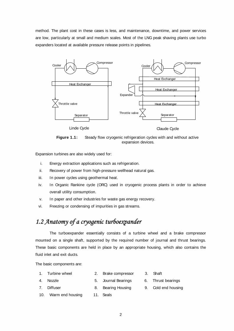
generate refrigeration. The steady flow cycles, with and without an active expansion device, have

been illustrated in Fig. 1.1. Compared to the high and medium pressure systems, turbine based

plants have the advantage of high thermodynamic efficiency, high reliability and easier

integration with other systems. The expansion turbine is the heart of a modern cryogenic

refrigeration or separation system. Cryogenic process plants may also use reciprocating

expanders in place of turbines. But with the improvement of reliability and efficiency of small

turbines, the use of reciprocating expanders has largely been discontinued.

In addition to their role in producing liquid cryogens, turboexpanders provide

refrigeration in a variety of other applications, such as generating refrigeration to provide air

conditioning in aeroplanes. In petrochemical industries, expansion turbine is used for the

separation of propane and heavier hydrocarbons from natural gas streams. It generates the low

temperature necessary for the recovery of ethane and does it with less expense than any other

2

method. The plant cost in these cases is less, and maintenance, downtime, and power services

are low, particularly at small and medium scales. Most of the LNG peak shaving plants use turbo

expanders located at available pressure release points in pipelines.

Heat Exchanger

Heat Exchanger

Heat Exchanger

Heat Exchanger

Cooler Cooler

Throttle valve

Throttle valve

Compressor Compressor

Separator Separator

Expander

Linde Cycle Claude Cycle

Figure 1.1: Steady flow cryogenic refrigeration cycles with and without active expansion devices.

Expansion turbines are also widely used for:

i. Energy extraction applications such as refrigeration.

ii. Recovery of power from high-pressure wellhead natural gas.

iii. In power cycles using geothermal heat.

iv. In Organic Rankine cycle (ORC) used in cryogenic process plants in order to achieve

overall utility consumption.

v. In paper and other industries for waste gas energy recovery.

vi. Freezing or condensing of impurities in gas streams.

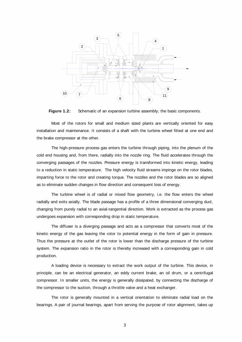
1.2 Anatomy of a cryogenic turboexpander

The turboexpander essentially consists of a turbine wheel and a brake compressor

mounted on a single shaft, supported by the required number of journal and thrust bearings.

These basic components are held in place by an appropriate housing, which also contains the

fluid inlet and exit ducts.

The basic components are:

1. Turbine wheel 2. Brake compressor 3. Shaft

4. Nozzle 5. Journal Bearings 6. Thrust bearings

7. Diffuser 8. Bearing Housing 9. Cold end housing

10. Warm end housing 11. Seals

3

10 78

11

9

4

5

6

3

2 1

Figure 1.2: Schematic of an expansion turbine assembly; the basic components.

Most of the rotors for small and medium sized plants are vertically oriented for easy

installation and maintenance. It consists of a shaft with the turbine wheel fitted at one end and

the brake compressor at the other.

The high-pressure process gas enters the turbine through piping, into the plenum of the

cold end housing and, from there, radially into the nozzle ring. The fluid accelerates through the

converging passages of the nozzles. Pressure energy is transformed into kinetic energy, leading

to a reduction in static temperature. The high velocity fluid streams impinge on the rotor blades,

imparting force to the rotor and creating torque. The nozzles and the rotor blades are so aligned

as to eliminate sudden changes in flow direction and consequent loss of energy.

The turbine wheel is of radial or mixed flow geometry, i.e. the flow enters the wheel

radially and exits axially. The blade passage has a profile of a three dimensional converging duct,

changing from purely radial to an axial-tangential direction. Work is extracted as the process gas

undergoes expansion with corresponding drop in static temperature.

The diffuser is a diverging passage and acts as a compressor that converts most of the

kinetic energy of the gas leaving the rotor to potential energy in the form of gain in pressure.

Thus the pressure at the outlet of the rotor is lower than the discharge pressure of the turbine

system. The expansion ratio in the rotor is thereby increased with a corresponding gain in cold

production.

A loading device is necessary to extract the work output of the turbine. This device, in

principle, can be an electrical generator, an eddy current brake, an oil drum, or a centrifugal

compressor. In smaller units, the energy is generally dissipated, by connecting the discharge of

the compressor to the suction, through a throttle valve and a heat exchanger.

The rotor is generally mounted in a vertical orientation to eliminate radial load on the

bearings. A pair of journal bearings, apart from serving the purpose of rotor alignment, takes up

4

the load due to residual imbalance. For horizontally oriented rotors, the journal bearings are

assigned with the additional duty of supporting the rotor weight. The shaft collar, along with the

thrust plates, form a pair of thrust bearings that take up the load due to the difference of

pressure between the turbine and the compressor ends. The thrust bearings in a vertically

oriented rotor additionally support the rotor weight.

The supporting structures mainly consist of the cold and the warm end housings with an

intermediate thermal isolation section. They support the static parts of the turbine assembly, such

as the bearings, the inlet and exit ducts and the speed and vibration probes. The cold end

housing is insulated to preserve the cold produced by the turbine.

1.3 Objectives of the present investigation Industrial gas manufactures in the technologically advanced countries have switched over

from the high-pressure Linde and medium pressure reciprocating engine based claude systems to

the modern, expansion turbine based, low pressure cycles several decades ago. Thus in modern

cryogenic plants a turboexpander is one of the most vital components- be it an air separation

plant or a small reverse Brayton cryocooler. Industrially advanced countries have already

perfected this technology and attained commercial success. However this technology has largely

remained proprietary in nature and is not available in open literature. To upgrade the technology

in air separation plants, as well as in helium and hydrogen liquefiers, it is necessary to develop an

indigenous technology for cryogenic turboexpanders.

For the development of turboexpander system this project has been initiated. The

objectives include: (i) building a knowledge base on cryogenic turboexpanders covering a range

of working fluids, pressure ratio and flow rate; (ii) construction of an experimental prototype and

study of its performance, and generation of specifications for indigenous development. The

development of the turbine involves several intricate technologies. Among the major components

of the system are: turbine wheel, braking device, gas bearings and pressure sealing. Each aspect

of the system has its own specific problems that have been specially addressed to.

For the experimental studies, a turboexpander system has been built with the following

specifications which are compatible with the compressor facility available in our laboratory:

Working fluid : Air/ Nitrogen

Turbine inlet temperature : 120 K

Turbine inlet pressure : 0.60 MPa

Discharge pressure : 0.15 MPa

Throughput : 67.5 nm3/hr

5

This thesis constitutes a portion of overall project on the study of cryogenic turboexpander

technology. The primary objectives of this investigation are:

• A comprehensive review of turboexpander literature

• Design and fabrication of basic units for the prototype turboexpander and

• Experimental and theoretical performance study of the turboexpander

1.4 Organization of the thesis

The thesis has been divided into eight chapters with one appendix. The first chapter

presents a brief introduction to expansion turbines and their application in cryogenic process

plants. The need for an indigenous development programme has been highlighted along with the

aim of the present investigation. Chapter–II presents an extensive survey of available literature

on various aspects of cryogenic turbine development. Starting with a comprehensive historical

profile, the chapter presents a brief outline of various technological issues related to design,

fabrication and testing.

The Chapter–III enunciates a systematic design procedure, based on published works

that has been developed and documented for all the components. The formal methodology has

been used to design a prototype turbine unit for fabrication and study. The specifications of this

system are based on the available air compressor. Full details of the design process, from

conception of the basic topology to preparation of production drawings and solid models have

been presented. In Chapter–IV, a parametric study has been carried out to determine the

optimum blade profile for given specifications. In Chapter–V attention has been paid to material

selection, tolerance analysis, fabrication and assembly of the turboexpander.

Chapter – VI describes the experimental set up to study the performance of the turbine.

This chapter presents the construction of the test rig including the air / nitrogen handling system,

bearing gas system, and instrumentation for measurement of temperature, pressure, rotational

speed and vibration. Experimental results for the prototype expander have also been included in

this chapter.

Prediction of performance under off-design conditions is an essential part of the design

process. The performance of a turbine system is expressed as a function of mass flow rate,

pressure ratio and rotational speed. Based on the available procedure, a one-dimensional

meanline analysis for estimating various losses and predicting the off design performance of an

expansion turbine has been discussed in Chapter–VII. Finally Chapter–VIII is confined to some

concluding remarks and for outlining the scope of future work.

Chapter 2

Literature Review

Chapter II

LITERATURE REVIEW

One of the main components of most cryogenic plants is the expansion turbine or the

turboexpander. Since the turboexpander plays the role of the main cold generator, its properties

– reliability and working efficiency, to a great extent, affect the cost effectiveness parameters of

the entire cryogenic plant.

Due to their extensive practical applications, the turboexpander has attracted the

attention of a large number of researchers over the years. Investigations involving applied as well

as fundamental research, experimental as well as theoretical studies, have been reported in

literature.

Fundamentals operating principles, design and construction procedures have been

discussed in well known textbooks on cryogenic engineering and turbomachinery [1–14]. The

books [1, 3, 4] provides an excellent introduction to the field of cryogenic engineering and

contain a valuable database on the turboexpander. The book by Devydov [5] contains lucid

description of the fundamentals of calculation and design procedure of small sized high speed

radial cryogenic turboexpander. The book by Bloch and Soares [6] is an up to date overview of

turboexpander and the processes where these machines are used in a modern, cost conscious

process plant environment. The detailed loss calculations and methods of performance analysis

are described by Whitfield and Baines [13, 14].

Journals such as Cryogenics and Turbomachinery and major conference proceedings such

as Advances in Cryogenic Engineering and proceedings of the International Cryogenic Engineering

Conference devote a sizable portion of their contents to research findings on turboexpander

technology.

2.1 History of development

The concept that an expansion turbine might be used in a cycle for the liquefaction of

gases was first introduced by Lord Rayleigh in a letter to “Nature” dated June 28, 1898 [15]. He

suggested the use of a turbine instead of a piston expander for the liquefaction of air. Rayleigh

emphasized that the most important function of the turbine would be the refrigeration produced

7

rather than the power recovered. In 1898, a British engineer named Edgar C. Thrupp patented a

simple liquefying machine using an expansion turbine [16]. Thrupp’s expander was a double-flow

device with cold air entering the centre and dividing into two oppositely flowing streams. At

about the same time, Joseph E. Johnson in USA patented an apparatus for liquefying gases. His

expander was a De Laval or single stage impulse turbine. Other early patents include expansion

turbines by Davis (1922). In 1934, a report was published on the first successful commercial

application for cryogenic expansion turbine at the Linde works in Germany [15]. The single stage

axial flow machine was used in a low pressure air liquefaction and separation cycle. It was

replaced two years later by an inward radial flow impulse turbine.

The earliest published description of a low temperature turboexpander was by Kapitza in

1939, in which he describes a turbine attaining 83% efficiency. It had an 8 cm Monel wheel with

straight blades and operated at 40,000 rpm [17]. In USA in 1942, under the sponsorship of the

National Defence Research Committee a turboexpander was developed which operated without

trouble for periods aggregating 2,500 hrs and attained an efficiency of more than 80% [17].

During Second World War the Germans used impulse type turboexpander in their oxygen plants

[18].

Work on the small gas bearing turboexpander commenced in the early fifties by Sixsmith

at Reading University on a machine for a small air liquefaction plant [19]. In 1958, the United

Kingdom Atomic Energy Authority developed a radial inward flow turbine for a nitrogen

production plant [20]. During 1958 to 1961 Stratos Division of Fairchild Aircraft Co. built blower

loaded turboexpanders, mostly for air separation service [18]. Voth et. al developed a high speed

turbine expander as a part of a cold moderator refrigerator for the Argonne National Laboratory

(ANL) [21]. The first commercial turbine using helium was operated in 1964 in a refrigerator that

produced 73 W at 3 K for the Rutherford helium bubble chamber [19].

A high speed turboalternator was developed by General Electric Company, New York in

1968, which ran on a practical gas bearing system capable of operating at cryogenic temperature

with low loss [22–23]. National Bureau of Standards at Boulder, Colorado [24] developed a

turbine of shaft diameter of 8 mm. The turbine operated at a speed of 600,000 rpm at 30 K inlet

temperature. In 1974, Sulzer Brothers, Switzerland developed a turboexpander for cryogenic

plants with self acting gas bearings [25]. In 1981, Cryostar, Switzerland started a development

program together with a magnetic bearing manufacturer to develop a cryogenic turboexpander

incorporating active magnetic bearing in both radial and axial direction [26]. In 1984, the

prototype turboexpander of medium size underwent extensive experimental testing in a nitrogen

liquefier. Izumi et. al [27] at Hitachi, Ltd., Japan developed a micro turboexpander for a small

helium refrigerator based on Claude cycle. The turboexpander consisted of a radial inward flow

reaction turbine and a centrifugal brake fan on the lower and upper ends of a shaft supported by

self acting gas bearings. The diameter of the turbine wheel was 6mm and the shaft diameter was

8

4 mm. The rotational speeds of the 1st and 2nd stage turboexpander were 816,000 and 519,000

rpm respectively.

A simple method sufficient for the design of a high efficiency expansion turbine is

outlined by Kun et. al [28–30]. A study was initiated in 1979 to survey operating plants and

generate the cost factors relating to turbine by Kun & Sentz [29]. Sixsmith et. al. [31] in

collaboration with Goddard Space Flight Centre of NASA, developed miniature turbines for

Brayton Cycle cryocoolers. They have developed of a turbine, 1.5 mm in diameter rotating at a

speed of approximately one million rpm [32].

Yang et. al [33] developed a two stage miniature expansion turbine made for an 1.5 L/hr

helium liquefier at the Cryogenic Engineering Laboratory of the Chinese Academy of Sciences.

The turbines rotated at more than 500,000 rpm. The design of a small, high speed turboexpander

was taken up by the National Bureau of Standards (NBS) USA. The first expander operated at

600,000 rpm in externally pressurized gas bearings [34]. The turboexpander developed by Kate

et. al [35] was with variable flow capacity mechanism (an adjustable turbine), which had the

capacity of controlling the refrigerating power by using the variable nozzle vane height.

A wet type helium turboexpander with expected adiabatic efficiency of 70% was

developed by the Naka Fusion Research Centre affiliated to the Japan Atomic Energy Institute

[36–37]. The turboexpander consists of a 40 mm shaft, 59 mm impeller diameter and self acting

gas journal and thrust bearings [36]. Ino et. al [38–39] developed a high expansion ratio radial

inflow turbine for a helium liquefier of 100 L/hr capacity for use with a 70 MW superconductive

generator.

Davydenkov et. al [40] developed a new turboexpander with foil bearings for a cryogenic

helium plants in Moscow, Russia. The maximum rotational speed of the rotor was 240,000 rpm

with the shaft diameter of 16 mm. The turboexpander third stage was designed and

manufactured in 1991, for the gas expansion machine regime, by “Cryogenmash” [41]. Each

stage of the turboexpander design was similar, differing from each other by dimensions only

produced by “Heliummash” [41].

The ACD company incorporated gas lubricated hydrodynamic foil bearings into a TC–3000

turboexpander [42]. Detailed specifications of the different modules of turboexpander developed

by the company have been given in tabular format in Reference [43]. Several Cryogenic

Industries has been involved with this technology for many years including Mafi-Trench.

Agahi et. al. [44–45] have explained the design process of the turboexpander utilizing

modern technology, such as Computational Fluid Dynamic software, Computer Numerical Control

Technology and Holographic Techniques to further improve an already impressive turboexpander

efficiency performance. Improvements in analytical techniques, bearing technology and design

features have made turboexpanders to be designed and operated at more favourable conditions

9

such as higher rotational speeds. A Sulzer dry turboexpander, Creare wet turboexpander and IHI

centrifugal cold compressor were installed and operated for about 8000 hrs in the Fermi National

Accelerator Laboratory, USA [46]. This Accelerator Division/Cryogenics department is responsible

for the maintenance and operation of both the Central Helium Liquefier (CHL) and the system of

24 satellite refrigerators which provide 4.5 K refrigeration to the magnets of the Tevatron

Synchrotron. Theses expanders have achieved 70% efficiency and are well integrated with the

existing system.

Sixsmith et. al. [47] at Creare Inc., USA developed a small wet turbine for a helium

liquefier set up at the particle accelerator of Fermi National laboratory. The expander shaft was

supported in pressurized gas bearings and had a 4.76 mm turbine rotor at the cold end and a

12.7 mm brake compressor at the warm end. The expander had a design speed of 384,000 rpm

and a design cooling capacity of 444 Watts. Xiong et. al. [48] at the institute of cryogenic

Engineering, China developed a cryogenic turboexpander with a rotor of 103 mm long and

weighing 0.9 N, which had a working speed up to 230,000 rpm. The turboexpander was

experimented with two types of gas lubricated foil journal bearings. The L’Air liquid company of

France has been manufacturing cryogenic expansion turbines for 30 years and more than 350

turboexpanders are operating worldwide, installed on both industrial plants and research

institutes [49, 50]. These turbines are characterized by the use of hydrostatic gas bearings,

providing unique reliability with a measured Mean Time between failures of 45,000 hours. Atlas

Copco [51] has manufactured turboexpanders with active magnetic bearings as an alternative to

conventional oil bearing system for many applications.

India has been lagging behind the rest of the world in this field of research and

development. Still, significant progress has been made during the past two decades. In CMERI

Durgapur, Jadeja et. al [52–54] developed an inward flow radial turbine supported on gas

bearings for cryogenic plants. The device gave stable rotation at about 40,000 rpm. The

programme was, however, discontinued before any significant progress could be achieved.

Another programme at IIT Kharagpur developed a turboexpander unit by using aerostatic thrust

and journal bearings which had a working speed up to 80,000 rpm. The detailed summary of

technical features of the cryogenic turboexpander developed in various laboratories has been

given in the PhD dissertation of Ghosh [55]. Recently Cryogenic Technology Division, BARC

developed Helium refrigerator capable of producing 1 kW at 20K temperature.

2.2 Design of turboexpander The process of designing turbomachines is very seldom straightforward. The final design

is usually the result of several engineering disciplines: fluid dynamics, stress analysis, mechanical

vibration, tribology, controls, mechanical design and fabrication. The process design parameters

which specify a selection are the flow rate, gas compositions, inlet pressure, inlet temperature

10

and outlet pressure [56]. This section on design and development of turboexpander intends to

explore the basic components of a turboexpander.

Turbine wheel During the past two decades, performance chart has become commonly accepted mode

of presenting characteristics of turbomachines [57]. Several characteristic values are used for

defining significant performance criteria of turbomachines, such as turbine velocity ratio0C

U ,

pressure ratio, flow coefficient factor and specific speed [58]. Balje has presented a simplified

method for computing the efficiency of radial turbomachines and for calculating their

characteristics [59]. Similarity considerations offer a convenient and practical method to recognize

major characteristics of turbomachinery. Similarity principles state that two parameters are

adequate to determine major dimensions as well as the inlet and exit velocity triangles of the

turbine wheel. The specific speed and the specific diameter completely define dynamic similarity.

The physical meaning of the parameter pair ss dn , is that, fixed values of specific speed sn and

specific diameter sd define that combination of operating parameters which permit similar flow

conditions to exist in geometrically similar turbomachines [8].

Specific speed and specific diameter The concept of specific speed was first introduced for classifying hydraulic machines.

Balje [58] introduced this parameter in design of gas turbines and compressors. Values of specific

speed and specific diameter may be selected for getting the highest possible polytropic efficiency

and to complete the optimum geometry [56]. Specific speed is a useful single parameter

description of the design point of a compressible flow rotodynamic machine [60]. A design chart

that has been used for a wide variety of turbomachinery has been given by Balje [8, 58, 61]. The

diagram helps in computing the maximum obtainable efficiency and the optimum design

geometry in terms of specific speed and specific diameter for constant Reynolds number and

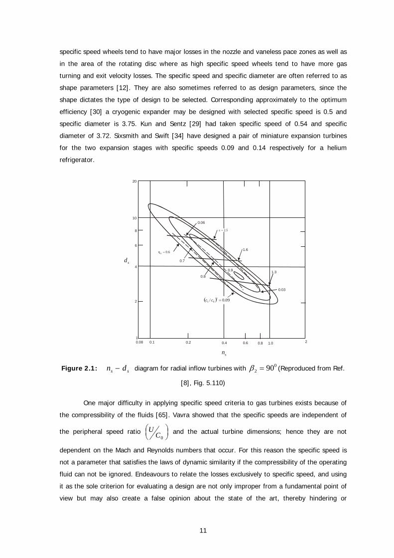
Laval number [8]. A, ss dn − diagram for radial inflow turbines of the mixed flow type, with a

rotor blade angle of 90° is reproduced in Fig 2.1.

A major advantage of Balje’s representation is that the efficiency is shown as a function

of parameters which are of immediate concern to the designer viz. angular speed and rotor

diameter. The ss dn − diagram given by Balje [8] has been obtained for a specific heat ratio

γ = 1.41. If the working fluid has a different value of γ (e.g. 1.67 for helium) the chart has to

be modified. Macchi [62] has shown that this effect is negligible for small pressure ratios, but

becomes significant at higher values.

According to Rohlik [63], for radial flow geometry, maximum static and total efficiencies

occur at specific speed values of 0.58 and 0.93.In reference [8] total to static efficiencies are

plotted for specific speeds ranging between 0.46 and 0.63. Luybli and Filippi [64] state that low

11

specific speed wheels tend to have major losses in the nozzle and vaneless pace zones as well as

in the area of the rotating disc where as high specific speed wheels tend to have more gas

turning and exit velocity losses. The specific speed and specific diameter are often referred to as

shape parameters [12]. They are also sometimes referred to as design parameters, since the

shape dictates the type of design to be selected. Corresponding approximately to the optimum

efficiency [30] a cryogenic expander may be designed with selected specific speed is 0.5 and

specific diameter is 3.75. Kun and Sentz [29] had taken specific speed of 0.54 and specific

diameter of 3.72. Sixsmith and Swift [34] have designed a pair of miniature expansion turbines

for the two expansion stages with specific speeds 0.09 and 0.14 respectively for a helium

refrigerator.

1.6

1.3

0.03

0.9

0.8

0.7

0.06

20

10

8

4

2

1

6

0.08 0.1 0.2 0.4 0.6 0.8 1.0 2

5.2=ε

6.0=stη

sn

sd

( ) 09.0/ 203 =cc

Figure 2.1: ss dn − diagram for radial inflow turbines with 02 90=β (Reproduced from Ref.

[8], Fig. 5.110)

One major difficulty in applying specific speed criteria to gas turbines exists because of

the compressibility of the fluids [65]. Vavra showed that the specific speeds are independent of

the peripheral speed ratio ⎟⎠⎞⎜

⎝⎛

0CU and the actual turbine dimensions; hence they are not

dependent on the Mach and Reynolds numbers that occur. For this reason the specific speed is

not a parameter that satisfies the laws of dynamic similarity if the compressibility of the operating

fluid can not be ignored. Endeavours to relate the losses exclusively to specific speed, and using

it as the sole criterion for evaluating a design are not only improper from a fundamental point of

view but may also create a false opinion about the state of the art, thereby hindering or

12

preventing research work that establishes sound design criteria. Vabra [65] has suggested

improvement of these charts by incorporating new data obtained through experiments. He has

shown that optimum turbine performance can be expected at values of specific speed between

0.6 and 0.7 and the operating range for radial turbines may lie between specific speed values of

0.4 to 1.2.

Parameters The ratio of exit tip to rotor inlet diameter should be limited to a maximum value of 0.7

to avoid excessive shroud curvature. Similarly, the exit hub to the tip diameter ratio should have

a minimum value of 0.4 to avoid excessive hub blade blockage and loss [63, 60]. Kun and Sentz

[29] have taken 68.0=ε . Balje [59] has taken the ratio of exit meridian diameter to inlet

diameter of a radial impeller as 0.625. The inlet blade height to inlet blade diameter of the

turbine wheel would lie between values of 0.02 to 0.6 [60]. The detailed design parameters for a

90° inward radial flow turbine is shown in Table 2.2 of the PhD dissertation of Ghosh [55].

The peripheral component of absolute velocity at the inlet of turbine wheel is mainly

dependent upon the nozzle angle. The peripheral component of absolute velocity at the exit of

turbine wheel is a function of the exit blade angle and the peripheral speed at the outlet [59].

Balje [59] shows that the desirable ratio of meridional component of absolute velocity at the inlet

and exit of the turbine wheel is a function of the flow factor and Mach number. He has taken the

value of the ratio of meridional components of absolute velocity at exit and inlet for a radial

turbine as 1.0. Whitfield [66] has shown that for any given incidence angle, the absolute flow

angle can be selected to minimize the absolute Mach number. The general view is that the

optimum incidence angle is a function of the number of blades and lies between -20° and -30°.

The absolute flow angle can then be selected to minimize the inlet Mach number, or alternatively

derived through the specification of the isentropic velocity ratio ⎟⎠⎞⎜

⎝⎛

0CU , as 0.7. The absolute flow

angle is usually selected to lie between 70° and 80°.

Number of blades Assuming a simplified blade loading distribution, Balje [8] has derived an equation for the

minimum rotor blade number as a function of specific speed. Denton [67] has given guidance on

the choice of number of blades. By using his theory it can be ensured that the flow does not

stagnate on the pressure surface. He suggests that a number of 12 blades is typical for cryogenic

turbine wheels. Wallace [68] has given some useful information on best number of blades to

avoid excessive frictional loss on the one hand and excessive variation of flow conditions between

adjacent blades on the other.

Rohlik [63] recommends a procedure to estimate the required number of blades

considering the criterion of flow separation in the rotor passage. In his formula, the number of

blades is chosen so as to inhibit boundary layer growth in the flow passage. Sixsmith [24] used

13

twelve complete blades and twelve partial blades in his turbine designed for medium size helium

liquefiers. The blade number is calculated from the value of slip factor [52]. The number of

blades must be so adjusted that the blade width and thickness can be manufactured with the

available machine tools.

Nozzle

A set of static nozzles must be provided around the turbine wheel to generate the

required inlet velocity and swirl. The flow is subsonic, the absolute Mach number being around

0.95. Filippi [64] has derived the effect of nozzle geometry on stage efficiency by a comparative

discussion of three nozzle styles: fixed nozzles, adjustable nozzles with a centre pivot and

adjustable nozzles with a trailing edge pivot. At design point operation, fixed nozzles yield the

best overall efficiency. Nozzles should be located at the optimal radial location from the wheel to

minimize vaneless space loss and the effect of nozzle wakes on impeller performance. Fixed

nozzle shapes can be optimized by rounding the noses of nozzle vanes and are directionally

oriented for minimal incidence angle loss.

The throat of the nozzle has an important influence on turbine performance and must be

sized to pass the required mass flow rate at design conditions. Converging–diverging nozzles,

giving supersonic flow are not generally recommended for radial turbines [13]. The exit flow

angle and exit velocity from nozzle are determined by the angular momentum required at rotor

inlet and by the continuity equation. The throat velocity should be similar to the stator exit

velocity and this determines the throat area by continuity [67]. Turbine nozzles designed for

subsonic and slightly supersonic flow are drilled and reamed for straight holes inclined at proper

nozzle outlet angle [69]. In small turbines, there is little space for drilling holes; therefore two

dimensional passages of appropriate geometry are milled on a nozzle ring. The nozzle inlet is

rounded off to reduce frictional losses.

Kato et. al. [35] have developed a large helium turboexpander with variable capacity by

varying nozzle throat and the flow angle of gas entering the turbine blade by rotating the nozzle

vanes around pivot pins. Ino et. al. [38] have derived a conformal transformation method to

amend the nozzle setting angle using air as a medium under normal and high temperature

conditions.

Mafi Trench Corporation [70] has invented a nozzle design that withstands full expander

inlet pressure and can be adjusted to control admission over a range of approximately 0 to 125%

of the design mass flow rate. The variable area nozzles act as a flow control device that provides

high efficiency over a wide range of flow [44].

Thomas [71] used the inlet nozzle of adjustable type. In this design the nozzle area is

adjusted by widening the flow passages. The efficiency of a well designed nozzle ring should be

about 95% while the overall efficiency of the turbine may be about 80% [24].

14

Vaneless space The space between the nozzle and the rotor, known as the vaneless space, has an

important role on turbine design. In the annular space between the nozzles and the rotor, the gas

flows with constant angular momentum, i.e., it is a free vortex flow. Consequently the velocity at

the mid point of the nozzle outlets should be less than the velocity at the rotor inlets in the ratio

of the two radii [24]. Watanabe et. al. [72] empirically determined the value of an interspace

parameter for the maximum efficiency. Whitfield and Baines [13] have concluded from others’

observations that the design of vaneless space is a compromise between fluid friction and nozzle-

rotor interaction.

Diffuser

The design of the exhaust diffuser is a difficult task, because the velocity field at the inlet

of the diffuser (discharge from the wheel) is hardly known. The diffuser acts as a compressor,

converting most of the kinetic energy in the gas leaving the rotor to potential energy in the form

of pressure rise. The expansion ratio in the rotor is thereby increased with a corresponding gain

in efficiency.

The efficiency of a diffuser may be defined as the fraction of the inlet kinetic energy that

gets converted to gain in static pressure. The Reynolds number based on the inlet diameter

normally remains around 105. The efficiency of a conical diffuser with regular inlet conditions is

about 90% and is obtained for a semi cone angle of around 5° to 6°. According to Shepherd, the

optimum semi cone angle lies in the range of 3°-5° [24]. A higher cone angle leads to a shorter

diffuser and hence lower frictional loss, but enhances the chance of flow separation. Whitefield

and Baines [13] and Balje [8] have given design charts showing the pressure recovery factor

against geometrical parameters of the diffuser.

Ino et. al. [38] have given the following recommendation for an effective design of the

diffuser: Half cone angle : 5° - 6° Aspect ratio : 1.4 – 3.3.

The inner radius is chosen to be 5% greater than the impeller tip radius and the exit radius of the

diffuser is chosen to be about 40% greater than the impeller tip radius [73], this proportion being

roughly representative of what is acceptable in a small aero turbine application.

It has further been suggested that the exit diameter of the diffuser may be obtained by

setting the exhaust velocity around 10–20 m/s. 30 to 40 percent of the residual energy, which

contains 4 to 5 percent of the total energy, can generally be recovered by a well designed

downstream diffuser [74]. Kun and Sentz [29] have described the gross dimensions of the

diffuser starting from the eye geometry, the remaining space envelope and the diffuser discharge

piping.

15

Shaft The force acting on the turbine shaft due to the revolution of its mass center and around

its geometrical center constitutes the major inertia force. A restoring force equivalent to a spring

force for small displacements, and viscous forces between the gas and the shaft surface, [75] act

as spring and damper to the rotating system. The film stiffness depends on the relative position

of the shaft with respect to the bearing and is symmetrical with the center-to-center vector.

Winterbone [76] has suggested that the diameter of the shaft be made the same as the

diameter of the turbine wheel, thus eliminating the need for a heavily loaded thrust bearing.

Shaft speed is limited by the first critical speed in bending [31, 70]. This limitation for a given

diameter determines the shaft length, and the overhang distance into the cold end, which

strongly affects the conductive heat leak penalty to the cold end. In practice, particularly in small

and medium size turbines, the bending critical speeds are for above the operating speeds. On the

other hand, rigid body vibrations lead to resonance at lower speeds, the frequencies being

determined by bearing stiffness and rotor inertia. Thomas [71] stated that the shaft and impellers

should be properly balanced. They used a dynamically balanced shaft of 3 mg imbalance on a

radius of 20 mm.

Brake compressor

The power developed in the expanders may be absorbed by a geared generator, oil

pump, viscous oil brake or blower wheel [77]. Where relatively large amounts of power are

involved, the generator provides the most effective means of recovery. Induction motors running

at slightly above their synchronous speed have been successfully used for this service. This does

not permit speed variation which may be desirable during plant start up or part load operation.

A popular loading device at lower power levels is the centrifugal compressor [2]. Because

of its simplicity and ease of control the centrifugal compressor is ideally suited for the loading of

small turbines. It has the additional advantage that it can operate at high speeds. For small

turbines whose work output exceeds the capacity of a centrifugal gas compressor, an electrical or

oil brake may be used. The electrical device may be an eddy current brake or permanent magnet

alternator, the latter having the advantage that heat is generated in an external load.

The power generated by the turbine is absorbed by means of a centrifugal blower which

acts as a brake [24, 47, 76, 78]. The helium gas in the brake circuit is circulated by the blower

through a water cooled heat exchanger and a throttle valve. The throttle valve is used to adjust

the load on the blower and the corresponding speed of the shaft. The blower is over-designed so

that when the throttle is fully open the shaft speed is less than the optimum value. The heat

exchanger removes the heat energy equivalent of the shaft work generated by the turbine from

the system. Thus the turbine removes heat from the process gas and transfers it to the cooling

water.

16

Design of brake compressors has not been discussed to any depth in open literature.

Jekat [69] has designed the load absorber as a single stage radially vaned compressor directly

coupled to the turbine by means of a floating shaft. The compression ratio ranges between 1.2

and 2.5 depending upon the speed.

The turboexpander brake assembly is designed in the form of a centrifugal wheel of

diameter 11.5 mm with a control valve at the inlet which provides for variation in rotor speed

within 20% [79]. The heat of friction is removed by the flow of lubricant through the static gas

bearings thereby ensuring constant temperature of the parts supporting the rotor. Most authors

[29] have followed the same guidelines for designing their compressors as for the turbine wheels.

Bearings Aerostatic thrust bearings

Decades of experience with cryogenic turboexpanders of various designs have shown

that the gas bearing is ideally suited for supporting the rotors of these machines. Kun, Amman

and Scofield [80] describe the development of a cryogenic expansion turbine supported on gas

bearings at the Linde division of the Union Carbide Corporation, USA during the mid and late

1960’s. They used aerostatic bearings to support the shaft.

L’Air Liquide of France began its developmental efforts on cryogenic turboexpander from

the late 1960’s [81]. Gas lubricated journal and thrust bearings were designed to support the

high-speed rotor. This bearing system assured an unlimited life to the rotating system, due to

total elimination of contact between the parts in relative motion.

In recent times, Thomas [71] has reported the development of a helium turbine with flow

rate of 190 g/s, working within the pressure limits of 15 and 4.5 bar. Both the journal as well as

the thrust bearings used process gas for external pressurisation. The journal bearings with L/D

ratio of 1.5 were designed for a shaft of diameter 25.4 mm. The bearing clearance was kept

within 20 and 25 μm. The bearing stiffness was measured to be 1.75 N/μm.

Sponsored by the Agency of Industrial Science and Technology of MITI, Japan, in early

1990’s, Ino, Machida and co-workers [38, 39] developed an expander for a liquefier capable of

liquefying helium at a rate of 100 lt/hr. The turbine was expected to run at 2,30,000 r/min. A

shaft-bearing system comprising of a pair of tilting pad journal bearings and a reliable externally

pressurised thrust bearing was developed. Annular collar thrust bearings with multi-feeding holes

were also developed to support the large thrust load resulting from the high expansion ratio of

the turbine.

Kun et. al. [75] have presented the development of a gas lubricated thrust bearing for

cryogenic expansion turbines. Kun et. al. [80] also describes results associated with the

development of gas bearing supported cryogenic turbines.

17

A high speed expansion turbine has been built by using aerostatic bearings as part of a

cold refrigerator for the Argonne National Laboratory (ANL) [21]. It is imperative that the turbine

receives a supply of bearing gas at all times during shaft rotation. The turbine, therefore, has

been supplied with a separate emergency supply for continuous operation.

Tilting pad journal bearings Sulzer Brothers, Switzerland [82] were the first company to sell cryogenic turboexpanders

supported on aerodynamic journal and thrust bearings. They initiated their development program

in the 1950’s. Early designs involved oil lubricated bearings. Later, the radial oil bearings were

replaced by a special type of self-acting tilting pad gas bearings invented by Hanny and Trepp

[15]. Their journal bearings [25] have three self-acting tilting pads. In this design, a converging

film forms between the pads and the shaft and generates the required pressure for supporting

the radial load. A fraction of the bearing gas from each converging film is fed to the back of the

pad, thus forming a film between the pad and the housing. The pad floats on this film of gas.

This tilting pad bearing is characterised by the absence of pivots in any form.

Sixsmith and his team at Creare Inc, USA developed a miniature tilting pad gas bearing

for use in very small cryogenic turboexpanders [34, 83]. They developed bearings with shaft

diameters down to about 3 mm and rotational speeds up to one million r/min, which were

suitable for refrigeration rates down to about 10 W.

The Japanese researchers joined the race for developing micro turbine technology by

using both the conventional tilting pad journal bearings as well as a grooved self acting bearing

giving successful operation up to 8,50,000 r/min [27]. The tests with tilting pad bearings did not

show any sign of shaft whirl. Vibration levels were always less than 3 microns.

Ino, Machida and co-workers [38, 39] developed an expansion turbine for a helium

liquefier with design speed of 2,30,000 r/min. The bearing system comprised of a pair of tilting

pad journal bearings and a reliable externally pressurised thrust bearing. The tilting pad journal

bearings were very stable and the shaft could be run up to the design speed without

encountering any problem. They used hardened Martensitic stainless steel (JIS SUS 440C) for the

shaft and a ceramic material for the tilting pads to prevent the seizure of the bearings during

start-stop cycles. The bearings could survive 200 start stop cycles without any problem.

Gas lubricated tilting pad journal bearings were also used to support the rotor of a large

helium turboexpander developed by the Japan Atomic Energy Research Institute and the Kobe

Steel Limited [35]. Agahi, Ershaghi and Lin [44] reported the development of a variant of

conventional tilting pad bearings – the flexible pad or flexure pivot bearing for supporting

cryogenic turboexpanders meant for hydrogen and helium liquefiers.

The Japan Atomic Energy Research Institute (JAERI) [36] has developed a turboexpander

consists of self acting tilting pad journal bearings for use on an experimental fusion reactor in

18

collaboration with Kobe Steel Ltd. Mafi Trench Corporation [70] designed and manufactured all its

own tilting pad journal bearings made of brass with a Babbitt lining. A detailed mathematical

analysis has been given in the PhD dissertation of Chakraborty [84] for tilting pad journal

bearings.

Seals

Proper sealing of process gas, especially in a small turboexpander, is a very important

factor in improving machine performance. For lightweight, high speed turbomachinery,

requirements are somewhat different from heavy stationary steam turbines [57]. The most

common sealing systems are labyrinth type, floating carbon rings, and dynamic dry face seals.

Due to extreme cold temperature, commercial dry face seal materials are not suitable for helium

and hydrogen expanders and a special design is needed. On the other hand, floating carbon rings

increase the shaft overhang and therefore limit the rotational speed. Considering the above, Agai

et. al. [44] have suggested the expander shaft seal to be a close noncontacting conical labyrinth

seal and the operating clearances to be of the order of 0.02 mm to 0.05 mm.

Effective shaft sealing is extremely important in turboexpanders since the power

expended on the refrigerant generally makes it quite valuable. Simple labyrinths can be used with

relatively good results where the differential pressure across the seal is low. More elaborate seals

are required where relatively high differential pressures must be handled. In larger machines,

static type oil seals have been used for these applications in which the oil pressure is controlled

by and balanced against the refrigerant pressure [77].

A major potential source of heat leak between the warm and the cold ends is due to the

flow of gas along the shaft. To minimize this leakage, the shaft extension from the lower bearing

to the turbine rotor is surrounded by a labyrinth seal [47]. It is essential that any flow of gas,

either upward or downward through this seal should be reduced to a minimum. An upward flow

will carry refrigeration out and a downward flow will carry heat in. In either case, there will be a

loss of efficiency. To minimize this loss a special buffer seal is provided.

Simple labyrinths running against carbon sleeves are employed as shaft seals. The

clearances used are in the magnitude of twice the bearing clearances. Serrations on the labyrinth

tips reduce the additional bearing load in case of rubbing [69]. Martin [69] first presented a

formula for the computation of the rate of flow through a labyrinth packing. The rapidly growing

size of turbomachinery market makes the investigation of relatively small losses worth while. In

this regard Geza Vermes [85] described a more accurate calculation procedure of leakage

through labyrinth seal.

The seal is exposed to the system pressure on one side and is ported to a regulated

supply of warm helium on the other side. Since pressure at the system side of the seal varies

depending on inlet conditions, Fuerest [46] have suggested the pressure at the other side must

19

be adjusted to maintain zero differential pressure across the seal. Mafi Trench Corporation [70]

used a spring loaded Teflon lip seal for sealing in cryogenic turboexpanders. Elastomeric ‘O’ rings

are used for sealing warm process casing and warm internal parts. Baranov et. al [41] and Voth

et. al. [21] have also used labyrinth seals on the shaft to reduce the leakage of gas.

2.3 Determination of blade profile Blade geometry

A method of computing blade profiles has been worked out by Hasselgruber [86], which

has been employed by Kun & Sentz [29] and by Balje [8, 87]. A complete aerodynamic analysis

of the flow path and structural analysis have been described by Bruce [88] for designing

turbomachinery rotor blade geometry. The rotor blade geometry is comprises of a series of three

dimensional streamlines which are determined from a series of mean line distributions and are

used to form the rotor blade surface. The profile distribution consists of radial and axial co-

ordinates that connect the inlet radii to the exit radii.

Wallace et. al. [89] describe a technique for designing mixed flow compressors which is

similar to that used by Wallace and Pasha for mixed flow turbines. Casey [90] used a new

computational method which used Bernstein Bezier polynomial patches to define the geometrical

shape of the flow channels.

The outside dimensions of the rotor and the casing as well as the blade angles are

determined from one dimensional design calculation [91, 92]. Strinning [93] has described a

computer program using straight forward design for completely specifying the shape of impellers

and guide vanes. A computer aided design method (CAD) has also been developed by Krain [94]

for radially ending and backswept centrifugal impellers by taking care of computational,

manufacturing, as well as aerodynamic aspects.

Parameters The complete design of a turbomachinery rotor requires aerodynamic analysis of the flow

path and structural analysis of the rotor including the blades and the hub. A typical rotor design

procedure follows the pattern of specifying blade and hub geometry, performing aerodynamic

and structural analysis, and iterating on geometry until acceptable aerodynamic and structural

criteria are achieved. This requires the geometry generation to focus not only on blade shape but

also on hub geometry.

In order to develop such a design system, it is critical that the rotor geometry generation

procedure be clearly understood. Rotor blade geometry end points are defined as the inlet and

exit radii, blade angles, and thickness. The rotor blade shape is determined by optimizing the

rotor blade distribution for aerodynamic performance and structural criteria are used to determine

20

the hub geometry. Rotor design procedures focus on generating geometry for both three

dimensional flow path analysis and structural analysis [88].

In seeking to find the most suitable geometry of radial turboexpander with the highest

possible efficiency, attention must be given to feasibility of constructing of the turboexpander.

Watanabe et. al. [72] have examined effects of dimensional parameters of impellers on

performance of the turbine. Similarly, Leyarovski et. al. [95] have done the optimization of

parameters for a low temperature radial centripetal turboexpander to determine the parameters

at which it would operate best.

Balje [87] has given a brief description of parameters influencing the curvature of the

flow path in the meridional and peripheral planes and consequently the boundary layer growth

and separation behavior of the flow path. He has followed a typical pressure balanced flow path

for optimization of the blade profile.

2.4 Development of prototype turboexpander Material selection Impellers

Aluminum is the ideal material for turbine impellers or blades because of its excellent low

temperature properties, high strength to weight ratio and adaptability to various fabrication

techniques. This material has been widely used in expanders either in cast form or machined

from forgings. Cast aluminum impellers for radial turbines may be safely operated at tip speeds of

200 to a maximum of about 300 metres per second, depending on the design [77]. Expander and

compressor wheels are usually constructed of high strength aluminum alloy. Low density and

relatively high strength aluminum alloys are ideally suited to these wheels as they operate at

moderate temperature with relatively clean gas. The low density alloy permits reducing the

weight of the wheels which is desirable to avoid critical speed problems [70] and centrifugal

stresses.

The turbine and compressor wheels can be produced by a variety of manufacturing

techniques. Aluminum alloys are used universally as the material, the major requirements for the

duty being high strength and low weight [2]. Clarke [19] has used aluminum alloy brake wheels

for his turboexpander. Akhtar [71] used the impeller as a precision investment casting of C-355-

T6 material.

The turbine rotor is made of high strength aluminium alloy. A rotor integral with the shaft

would be simpler, but it was found difficult to end mill the rotor channels in high tensile titanium

alloy [24]. With tip speeds up to 500 m/sec, titanium compressor wheels machined out of solid

forgings are standard industry practice [96]. Duralumin is ideal material for use in the rotor disk,

it has a high strength to weight ratio and is adaptable to various vibrating techniques.

21

Shaft The turbine rotor is mounted on an extension of the shaft, which overhangs into the cold

region. The material of the shaft is 410 stainless steel or K-monel. stainless steel 410 was chosen

because of its desirable combination of low thermal conductivity and high tensile strength [76]. In

designing the shaft bearing system, prevention of contact damage between the journal and

bearing at start up is very important. Shaft hardness and bearing material selection are therefore

important considerations. The experimental machine used hardening heat treated martensitic

stainless steel for the shaft and ceramic for the bearing [38]. The 18/8 stainless steel is also

frequently used as a shaft material since its low thermal conductivity is advantageous in limiting

heat flow into the cold region of the machine. It is necessary to treat the surface to improve its

bearing properties [2]. The particular shaft used is made of titanium to reduce heat leak [97].

The shaft is made from nitridied steel and hardened to 600 Bn on the bearing surfaces [71].

Bearings Prevention of contact damage between the journal and the bearing at start up is very

important. No flaws should be found in the contact surface of the bearing and the shaft. Ino et.

al. [38] found no flaws on the heat treated surface of the journal combined with the ceramic

tilting pads after 200 start/stop cycles and then it was confirmed that the combination of shaft

and ceramic bearing provides significant improvement in their contact damage.

Bearings are of nickel silver, used largely for ease of accurate machining and

compatibility with respect to its coefficient of contraction in cooling [19]. Halford et. al. [20] used

lead bronze for air bearings. The bearings made from SAE64 leaded bronze. This material is

selected for its anti friction properties which reduces scoring during initial testing [71].

Nozzle One of the disadvantages of the radial inward flow path is the tendency of foreign

particles to accumulate in the space between the nozzles and the wheel, causing surface damage

by erosion. In severe cases, the trailing edges of the nozzles have been completely worn away.

The use of stainless steel nozzles reduces the rate of deterioration but the only satisfactory cure

is the prevention of particle entry by filtration [2]. Swearingen [18] has suggested that the nozzle

must be of special material to withstand this erosion in order to have reasonable life. Cryogenic

turboexpanders, however, are essentially free of this problem because of the clean fluid that they

use.

Thomas [71] manufactured the nozzle from type 310 stainless steel. Fixed nozzles are of

nickel silver, used largely for ease of accurate machining and compatibility with respect to its

coefficient of contraction in cooling [19].

22

Housing In the choice of materials for the main body of the turbine, there was no difficulty with

chemical compatibility and the choice was based on strength and fatigue properties on the one

hand and adequate thermal properties of conductivity and expansion on the other [20].

Since it was necessary to keep the thermal conductivity to a minimum, the next step was

to decide on the actual body material. Normal design methods can reduce the cross sectional

area available for conduction to the absolute minimum, and a correlation of literature data on

thermal conductivity in the important temperature range shows a most significant difference in

characteristics between the aluminum alloys and pure metals on the one hand and stainless steel

on the other. The greatest potential source of heat conduction is through that portion of the body

which connects the low temperature end to the ambient temperature end. It was decided to bolt

this part to the outside of the cold box in a position providing ready accessibility. With a compact

design, the temperature gradient at the working conditions is quite steep, and stainless steel was

felt to be the most suitable material.

Materials with sufficient ductility at low temperature encountered have been selected. 18-

8 stainless steel is used for the rotating elements and the bearing housings. The various turbine

housings are of cast aluminum bronze. The thermal expansion coefficients of 18-8 stainless steel

and the selected grade of aluminum bronze are nearly the same. This makes for stability of fits

and alignment [69].

The main body of the turbines, which was originally constructed of brass and nickel

silver, has changed to of 18/8 stainless steel for manufacturing [19]. Similarly Thomas [71] used

the inlet housing as a weldment of 304 stainless steel. Stainless steel has the disadvantage of

cost and weight, so the casings at the warm end of the machine can advantageously be of

aluminum. In fact, medium sized turbines have been constructed using aluminum castings

throughout at a small penalty on efficiency [2]. The material of the turbine casing is the same 9%

Nickel steel as the rotor shaft so as not to allow a gap between the impeller and casing by

thermal contraction [37]. Housing of small turboexpander systems used in helium liquefiers is

almost universally made of stainless steel.

Seal Many different materials have been used for making turboexpander seals. Commercially

available cryogenic seals are used but not relied upon. The best commercially available cryogenic

reusable seals are made of rings of PTEE coated metals [19].

Labyrinth type seals are utilized between the expander and compressor wheels and the

oil or gas lubricated bearings. Shaft seals are labyrinth type to minimize seal gas leakage. The

design incorporates a replaceable stainless steel rotating labyrinth running adjacent to a fiber

reinforced phenolic seal cartridge [70]. The turbine rotor housing originally contained a carbon

23

labyrinth seal from the downstream side of the turbine, a device which was later found to be

redundant as the best seal is the closest fitting sleeve which is possible [20].

Labyrinth packing and an adjustable throttle are used for eliminating leaks between the

rotor support (hot) and cold zones [79]. While Voth et. al. [21] have reported the use of stainless

steel in their labyrinth seals, Sixsmith has recommended nickel silver to reduce heat conduction

[47].

Fabrication

As rotational speed is increased, wheel size is reduced. In small turboexpanders,

problems are related to miniaturization, Reynolds number effects, heat transfer, seals, bearing

and critical speed. When the wheel size is small, it is questionable whether the wheel can be

produced economically with the required accuracy necessary to reduce losses.

In a high speed expander, brazing of the wheel is not acceptable because of high tip

speeds. Wheel casting patterns are very expensive and very difficult to make, particularly for

small wheels when the surface of blade has an arbitrary shape that requires close tolerances

[45].

Interactive graphics assisted tool selection software has produced satisfactory geometries

for design specifications of turbine wheels. This computer program is intended for straight line

element blading and features optimal flank milling. A 5-axes CNC milling machine may be

employed to obtain the required profiles with close tolerances [45].

Thomas [71] used investment casting of C-355-T6 aluminium alloy to construct a

turboexpander at CCI Cryogenics, USA. Colyer [22] has produced impulse wheels and nozzles

from titanium by the three methods: a) direct milling of the wheel and the nozzles by tracing

from an enlarged pattern, b) electro-discharge machining, and c) diffusion bonding of photo-

etched laminations.

During the early years of cryogenic turbine development, when CNC machines were not

available, special purpose machines were used to fabricate turbine wheels. Brimingham et. al.

[76] constructed a specially designed pantograph for the purpose of machining the turbine rotor.

The designer has to choose a convenient balance between the needs of aerodynamic

performance, stress and vibration resistance [98]. A fixed radius fillet is usually the easiest to

machine, especially when the radius is the same as that of the tool, ideally suited to machining

the blade. Precision of manufacture is essential. Before assembly, the flatness and the run out of

the shaft disk have to be measured and they should not exceed 0.003 mm [25].

Balancing Only a few authors have described the balancing requirements of a cryogenic

turboexpander. Beasly and Halford [20] have suggested that shaft eccentricity equal to one tenth

24

of the radial bearing clearance is acceptable. Turbine rotors made by Mafi Trench Corporation,

USA are dynamically balanced to the specifications of ISO G 2.5 on precision electronic balancing

machines. Schimd [25] has recommended a maximum unbalance of 20 mg.cm for a rotor

weighing 300 g. Clarke [19] recommends acceptable unbalance of 0.75 mg.cm for the rotor of

BOC helium turbine. High speed dynamic balancing machines are available in international market

for balancing small rotors. The requirements of balancing can be reduced by choice of

homogenous material and precision fabrication of the cylindrical components with appropriate

tolerance on cylindricity.

Assembly

A prime requirement of expansion turbine design is the facility for easy replacement of

parts. The most popular structural arrangement is a modular system which has been followed by

most workers [19, 34, 47]. In this arrangement, the turbine assembly is constructed of an inner

module and an outer casing. The inner module consists of the rotating parts and the bearings.

The outer casing consists of the turbine housing, the flanges, the piping and sensor interfaces. In

case of a failure, the bearings and the rotor can be taken out and replaced without disturbing the

connections to the rest of the plant.

Small high speed turbines are generally designed with a vertical rotor. This eliminates

radial load on the journal bearings which have low load carrying capacity. The rotors being small

and light in weight, the thrust bearings can easily absorb both pressure and gravity loads. In

larger rotors, the operating speed is low, making it possible to use robust antifrictrion journal

bearings with significant load carrying capacity. Simultaneously, the increased rotor weight may

not be absorbed easily by the thrust bearings. Therefore larger turbines are better designed in a

horizontal configuration. In critical applications, vertical operation also helps in reducing the

convective heat leak in the gas space separating the warm and the cold ends of the machine

[47].

The expander was designed [47] to be flanged mounted on the top cover of a stand with

the shaft axis operating in a vertical position. Vertical operation is important to reduce convective

heat leaks in the gas spaces separating the warm and cold end of the machine. The inlet and

exhaust connections to the expander are made by means of bolted flanges incorporating static

seals. By using flange connections, the possibility of introducing contaminants (due to solder

fluxes or welding slag) can be eliminated. It also provides a quick and easy means of installing

and removing the turboexpander.

The turbine rotor, the shaft and brake impeller are manufactured as an integral piece

from high tensile strength titanium alloy. The journal bearing and lower side of the thrust bearing

are fabricated from a number of pieces which are silver soldered together to form an integral

assembly. This unit is machined to size after soldering. The assembly incorporates pneumatic

25

phase shift stabilizers against shaft whirl. The upper side of the thrust bearing is built into the

brake circuit assembly. Its function is to limit the axial play of the shaft and, if needed, to support

an upward thrust load [34].

2.5 Experimental performance study

The testing of turboexpanders depends, by necessity, on certain measurements to obtain

a quantitative evaluation of performance e.g. efficiency and power. The accurate measurement of

temperatures, flow rate, and pressures is significant in determining turbine efficiency. When

power measurement is needed, the flow rate becomes as critical as temperature [54, 99]. There

are various methods of indicating turbine performance. The isentropic and polytropic efficiencies

are very common in literature. Bearing gas consumption does not directly affect the turbine

performance but does reduce the overall efficiency of the cycle by about 20% [97]. For

performance measurements the turbine is usually equipped with conventional instrumentation to

measure turbine inlet and exit flow conditions and rotational speed [100].

Temperature measurement

Thermocouples are the preferred type of instrument for measurement of temperature

because of the simplicity of operation. They can attain a high levels of accuracy particularly while

measuring differences in temperature. They are also suitable for remote reading. Thermocouples

are usually robust and relatively inexpensive [54]. Kato et. al. [35] used Pt-Co resistance

thermometers with proven accuracy of less than 0.1K in the range from 20 to 300K. Futral &

Wasserbauer [101] measured the inlet stagnation temperature with a setup consisting of three

thermocouples. Germanium resistance thermometers have been used by Kato et. al. [37] at the

inlet and outlet piping.

Flow measurement

Flow rate measurement accuracies are just as important as those of temperature

measurement. When energy balance is required, the flow rate of the fluid is measured by an

orifice plate placed upstream of the turbine inlet and away from the flow disturbances (elbows,

bend etc.) [54].

Futral & Wasserbauer [101] measured flow rate with a sharp edged orifice that was

installed according to the ASME test code. Kato et. al. [37] has also used an orifice flow meter to

determine the mass flow rate. A venturi nozzle at upstream of the compressor has been used by

Came [73] to measure mass flow.

26

Pressure measurement The following instruments are used to measure pressures at different points in a turbine test

set up.

• Bourdon tube gauges

• Liquid manometers

• Pitot tubes

• Pressure transducers

Differential pressures and sub-atmospheric pressures are measured by manometers with a

fluid that is chemically stable. Mercury taps are used to prevent the manometric fluid from

entering process piping. Errors in these instruments are around 0.25% [54].

Two total pressure probes were also used by Futral and Wasserbauer [101] to determine the

turbine total pressure ratio. The turbine developed by Benisek [100] was instrumented with static

pressure taps to measure surface pressures around the circumference of the rotor inlet, as well

as in the meridional direction along the shroud contour from inlet to exit.

Speed measurement

During the early years of turbine development, speed was measured with and electronic

counter actuated by a magnetic pulse generator or a toothed gear attached to the shaft. But the

method of speed measurement was found to be inaccurate; so non-contacting type optical

probes are used by placing a strobolight on the shaft. The speed is recorded on a digital counter

[54]. A six tooth sprocket mounted on one end of the high speed coupling was used in

conjunction with a magnetic pickup and electronic tachometer to record speed [101].

To provide shaft stability and speed signal, a small proximity probe is located between

the brake rotor and the upper bearing. The clearance between the probe and the shaft is about

0.1 mm. An electronic circuit which is sensitive to small changes in capacitance provides a signal

which is approximately proportional to small displacements of the shaft towards or away from the

probe. The signal is displayed on the screen of an oscilloscope. Radial displacements from the

position of equilibrium down to about 0.2 micron can be observed [47]. To provide a speed

signal, a sharp spike is generated each time the flat passes the probe. An oscilloscope with a

calibrated sweep provides a display of both shaft stability and shaft speed [37, 46].

The speed of rotation is measured by a capacitance probe located over a flat on the

shaft. The signal is amplified and fed into a frequency meter for visual display. The turbine

normally operates at 240,000 rpm but can safely run at 300,000 rpm to accommodate changes in

refrigeration load [21]. A notched shaft and an eddy current probe were used to measure the

rotational speed of the rotor and to provide information relating the instantaneous blade position

to the laser measurement position [100].

27

The data on temperature, pressure, and flow rate were automatically observed and

recorded by pen recorders and the micro computer data acquisition system which can

immediately convert the voltage signals to physical quantities [35, 36].

Efficiency of turboexpander

Isentropic efficiency is generally used for representing temperature changes across a

cryogenic turbine. For preliminary design purposes it is necessary to assume the efficiency of

turbine. Denton [67] at Cambridge University assumed a turbine efficiency of 0.7 for a

turboexpander designed as an undergraduate project. Kanoglu [102] established a suitable model

for the assessment of cryogenic turbine performance. He studied the isentropic, hydraulic and

exergetic efficiencies and compared them with the output from a throttled valve. Gao et. al [103]

provide an optimized design method based on genetic algorithm to approximately choose the

main parameters that have significant effect on performance during the design process.

2.6 Off-design performance of turboexpander Meanline method

In order to achieve high efficiency of cryogenic turboexpanders, it is very important

during the design process to appropriately choose the main parameters that determine its

performance. A number of methods for representing the losses in radial gas turbines for

predicting off-design performance of a turboexpander are reviewed. It is shown that reasonable

predictions of the turbine performance may be made using one dimensional theory [104].

A meanline loss system is described that is capable of predicting the efficiency of radial

turbine stages at both on- and off-design conditions. The system is based on the well known

approach introduced by NASA in the 1960s [105]. Meanline, or one-dimensional, methods are

routinely used for the design and analysis of radial turbines. They are very fast to compute and

require only a small amount of geometric information. For these reasons they are extremely

useful in the initial stages of a design, and can be used to investigate very quickly a number of

different design options before any details of the blade geometry have been fixed. The principal

disadvantage of meanline methods is that some means of estimating the loss or efficiency of

individual components of the turbine must be available if realistic estimates of performance are to

be made.

A performance prediction program based on a one-dimensional analysis of expansion

turbines has been developed, on the basis of which a method of selecting similarity criteria to

deal with model tests on air and helium turbines is presented [106]. The method of performance

estimation based on the one dimensional flow theory for a wide range of nozzle angles of variable

geometry radial inflow turbine is presented. In this method it is assumed that turbine

performance at the design point and geometry of the components are given [107].

28

A modified report has been made for a radial inflow turbine to enhance the design code

capabilities consistent with those of a companion off-design code [108]. Liu et. al. [103] provide a

new type of optimization method which is based on the genetic algorithm.

Losses in turboexpander

Low specific speed wheels tend to have major losses in the nozzle and vaneless space

zones as well as in the rotating disc. High specific speed wheels tend to have more gas turning

and exit velocity losses. Analysis of the individual losses in a specific machine involves the effect

of Reynolds number, surface finish, density ratio, Mach number, clearance ratios and geometric

effects [64].

The physical size of the machine influences its efficiency since fluid friction losses

decrease with increasing Reynolds number. In addition, relative leakage losses can be reduced

for larger machines since clearance can usually be held to a smaller percentage of working

dimensions. Likewise, blade thickness losses and other imperfections incidental to manufacturing

become less critical for larger machines [77].

Balje [8] has considered the following losses in order to determine optimum geometry:

• Nozzle blade row boundary layers,

• Rotor passage boundary layers

• Rotor blade tip clearance

• Disc windage (on the back surface of the rotor)

• Kinetic energy loss at exit

The major sources of exergy loss may be divided into three groups, depending on their

variation with flow rate: losses due to nozzle end wall friction, and due to cylinder friction

between the shroud and the rotor, tip leakage, and heat in-leak [24]. A study was conducted by

Khalil et. al. to determine these losses experimentally and theoretically in radial inflow turbine

nozzles [109]. Experimental results were obtained for the flow at the inlet and exit of a full scale

radial turbine stator annulus. These experimental results were used to develop a better

theoretical model for loss prediction in the stator annulus.

Nozzle Loss Wasserbauer and Glassman [110] found from experiments that the ratio of total

stagnation pressures between the nozzle exit and inlet remains fairly constant, between 0.98 and

0.99, over a wide range of operating parameters. Hence they recommend the nozzle loss

coefficient to be defined in terms of stagnation pressure ratio across the nozzle.

The nozzle loss is minimum when the nozzle inlet Mach number is between 0.7 and 0.9

[111]. If the inlet angle of the relative velocity ( 1β ) is between 80° and 90°, there is no or

29

negligible inlet loss in the wheel. For all practical purposes a well designed nozzle segment may

be expected to have a loss coefficient of the order of 0.1 [104].

Rotor passage loss Accurate estimation of rotor passage loss is difficult. The viscous loss in a channel is

assumed to be proportional to the average kinetic energy in the channel, the average kinetic

energy being the average of kinetic energies entering and leaving the rotor[101]. Again the rotor

passage loss is modified by Wasserbauer and Glassman [110] to give a better correlation with

experimental data. Bridle and Boulter [104] used stagnation pressure loss to determine a

coefficient for the passage loss.

Rotor incidence loss One of the major losses that occur in radial inflow turbines is the impeller incidence loss

due to the variation between the impeller blade angle and relative inlet velocity at the impeller

tip. This incidence loss is due to the turbine speed being incorrect for the given process

conditions. Since the turbine speed is determined by the loading device, it is important to match

the loader to the turbine so that equilibrium operation occurs at optimum speed. It is generally

well known that the optimum velocity triangle at the wheel tip does not occur at zero incidence

but approaches the velocity triangle as determined by using the slip fator concept of centrifugal

compressor. Optimum incidence angle for a 90° impeller is approximately -20° [64, 66].

Whitfield [66] has shown that for an optimum incidence angle the absolute flow angle

can be selected to minimize the absolute Mach number. The minimum Mach number condition

should lead to the minimization of the stator losses. As this condition also leads to the minimum

relative Mach number, it should also be the condition for minimum rotor losses. The absolute flow

angle is usually selected to lie between 70° and 80°.

For calculating incidence loss at the rotor inlet, it is assumed that the loss is equivalent to

the kinetic energy of the velocity component normal to the blade at the rotor inlet [101]. The

combination of high wheel speed and low stator velocity will result in severe incidence losses and

a corresponding decrease in work in high speed and high pressure ratio range of operation. At

high speeds the radial machine shows a far greater increase in incidence loss.

Several loss models [8, 87, 110] have been proposed to describe incidence loss. Benson

[104] has shown that the incidence loss models proposed by Balje [8], Futral and Wasserbauer

[101], and Wallace [68] give almost identical results.

The incidence loss models proposed by NASA workers [101, 110] are widely used. Baines

[105] has, however, criticized these models on the ground that the physical reason behind the

concept of slip at the exit of a centrifugal impeller is different from that at the inlet of a radial

inflow turbine. In the former case, the secondary flow and its subsequent mixing with the main

stream are the primary causes of the slip, while in the case of the radial turbine, blade loading

30

and Coriolis acceleration are the major factors. It has been further suggested that the optimum

incidence angle has to be taken at the best efficiency point, and in the absence of any

experimental data, the best efficiency point may be taken where the blade to jet velocity ratio is

0.7.

Rotor clearance loss Turbine wheel clearance along the contour surface between the spinning wheel and the

stationary shroud allows a portion of the gas to slip through without delivering energy to the

wheel. This loss is known as clearance loss. Blade clearance is important because, even with very

small operating clearances, leakage losses in a miniature turbine can be a significant part of the

total flow. Wheel efficiency is based on total to total pressures and temperature differences

between inlet and exit; and the overall efficiency is based on net electrical output with all losses

included. The overall efficiency drops as the blade clearance is increased because the amount of

flow from the tip of the nozzle bypassing the wheel may be between 5 to 10 percent of the total

nozzle flow [22].

Rohlik [63] and Watanbe et. al. [72] has also arrived at a similar conclusion from their

experiences. They found that the radial clearance at the turbine exit is more serious than the

axial clearance. Ino et. al. [38] have observed that in small, high pressure ratio cryogenic

turbines, efficiency loss is considerable if the axial clearance ratio exceeds the value of 0.3. Kato

et. al. [36] have identified clearance losses to be the most prominent source of inefficiency in

large helium turboexpanders. They have suggested the use of shrouded rotors and labyrinth seals

to reduce clearance losses and improve overall efficiency.

Chapter 3

Design of Turboexpander

Chapter III

DESIGN OF TURBOEXPANDER

In this chapter the process of design of the experimental turboexpander and associated

units for cryogenic process have been analysed. The whole system consists of the turbine wheel,

nozzles, diffuser, shaft, brake compressor, journal and thrust bearings and the appropriate

housing. The design procedure of the cryogenic turboexpander depends on working fluid, flow

rate, inlet conditions and expansion ratio. The procedure created in this chapter allows any

arbitrary combination of fluid species, inlet conditions and expansion ratio, since the fluid

properties are adequately taken care in the relevant equations. The computational process is

illustrated with examples. The present design procedure is more systematic and lucid than

available in open literature [55]. The design methodology of the turboexpander system consists

of the following units, which are described in the subsequent sections.

• Fluid parameters and layout of the components,

• Design of turbine wheel,

• Design of diffuser and nozzle ,

• Design of brake compressor,

• Shaft design,

• Selection of bearings,

• Design of supporting structure

3.1 Fluid parameters and layout of components The fluid specifications have been dictated by the requirements of a small refrigerator

producing less than 1 KW of refrigeration. A turbine efficiency of 75% has been assumed

following the experience of the workers [20, 33, 67, 69]. The inlet temperature has been

specified rather arbitrarily, chosen in such a way that even with ideal (isentropic) expansion, the

exit state should not fall in the two-phase region. The basic input parameters for the system are

given in Table 3.1.

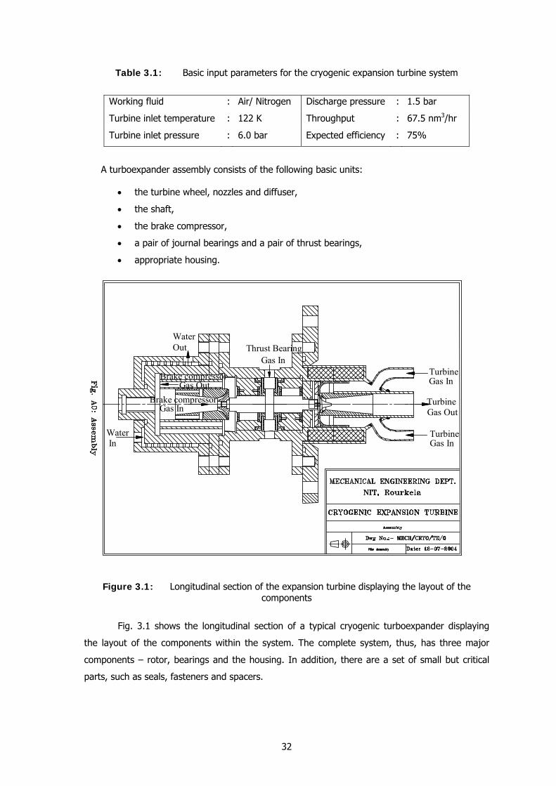
32

Table 3.1: Basic input parameters for the cryogenic expansion turbine system

Working fluid : Air/ Nitrogen Discharge pressure : 1.5 bar

Turbine inlet temperature : 122 K Throughput : 67.5 nm3/hr

Turbine inlet pressure : 6.0 bar Expected efficiency : 75%

A turboexpander assembly consists of the following basic units:

• the turbine wheel, nozzles and diffuser,

• the shaft,

• the brake compressor,

• a pair of journal bearings and a pair of thrust bearings,

• appropriate housing.

Figure 3.1: Longitudinal section of the expansion turbine displaying the layout of the components

Fig. 3.1 shows the longitudinal section of a typical cryogenic turboexpander displaying

the layout of the components within the system. The complete system, thus, has three major

components – rotor, bearings and the housing. In addition, there are a set of small but critical

parts, such as seals, fasteners and spacers.

Brake compressor Gas In

Brake compressor Gas Out

Thrust Bearing Gas In

Turbine Gas In

Turbine Gas In

Turbine Gas Out

Water In

Water Out

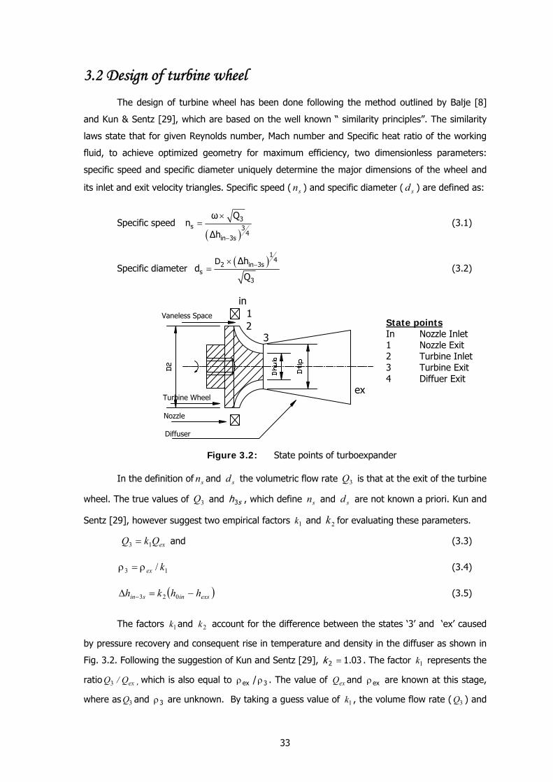
33

3.2 Design of turbine wheel The design of turbine wheel has been done following the method outlined by Balje [8]

and Kun & Sentz [29], which are based on the well known “ similarity principles”. The similarity

laws state that for given Reynolds number, Mach number and Specific heat ratio of the working

fluid, to achieve optimized geometry for maximum efficiency, two dimensionless parameters:

specific speed and specific diameter uniquely determine the major dimensions of the wheel and

its inlet and exit velocity triangles. Specific speed ( sn ) and specific diameter ( sd ) are defined as:

Specific speed ( )−

×= 3

s 34

in 3s

ω Qn

Δh (3.1)

Specific diameter ( )−×

=

14

2 in 3ss

3

D Δhd

Q (3.2)

Figure 3.2: State points of turboexpander

In the definition of sn and sd the volumetric flow rate 3Q is that at the exit of the turbine

wheel. The true values of 3Q and sh3 , which define sn and sd are not known a priori. Kun and

Sentz [29], however suggest two empirical factors 1k and 2k for evaluating these parameters.

exQkQ 13 = and (3.3)

13 / kexρ=ρ (3.4)

( )exsinsin hhkh −=Δ − 023 (3.5)

The factors 1k and 2k account for the difference between the states ‘3’ and ‘ex’ caused

by pressure recovery and consequent rise in temperature and density in the diffuser as shown in

Fig. 3.2. Following the suggestion of Kun and Sentz [29], 03.12 =k . The factor 1k represents the

ratio exQ/Q3 , which is also equal to 3ex /ρρ . The value of exQ and exρ are known at this stage,

where as 3Q and 3ρ are unknown. By taking a guess value of 1k , the volume flow rate ( 3Q ) and

Turbine Wheel

Diffuser

Nozzle

Vaneless Space 1in

23

ex

State points In Nozzle Inlet 1 Nozzle Exit 2 Turbine Inlet 3 Turbine Exit 4 Diffuer Exit

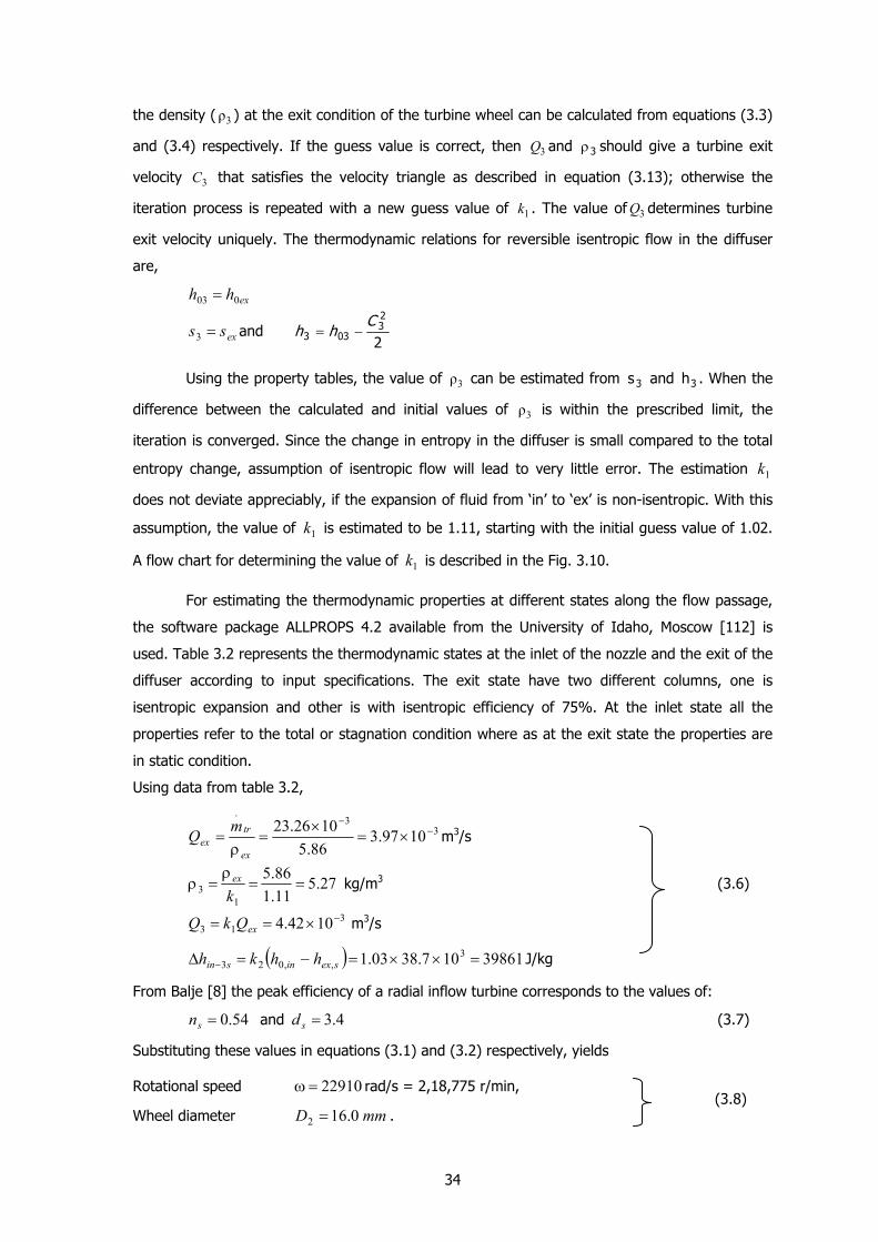
34

the density ( 3ρ ) at the exit condition of the turbine wheel can be calculated from equations (3.3)

and (3.4) respectively. If the guess value is correct, then 3Q and 3ρ should give a turbine exit

velocity 3C that satisfies the velocity triangle as described in equation (3.13); otherwise the

iteration process is repeated with a new guess value of 1k . The value of 3Q determines turbine

exit velocity uniquely. The thermodynamic relations for reversible isentropic flow in the diffuser

are,

exhh 003 =

exss =3 and 2

23

033C

hh −=

Using the property tables, the value of 3ρ can be estimated from 3s and 3h . When the

difference between the calculated and initial values of 3ρ is within the prescribed limit, the

iteration is converged. Since the change in entropy in the diffuser is small compared to the total

entropy change, assumption of isentropic flow will lead to very little error. The estimation 1k

does not deviate appreciably, if the expansion of fluid from ‘in’ to ‘ex’ is non-isentropic. With this

assumption, the value of 1k is estimated to be 1.11, starting with the initial guess value of 1.02.

A flow chart for determining the value of 1k is described in the Fig. 3.10.

For estimating the thermodynamic properties at different states along the flow passage,

the software package ALLPROPS 4.2 available from the University of Idaho, Moscow [112] is

used. Table 3.2 represents the thermodynamic states at the inlet of the nozzle and the exit of the

diffuser according to input specifications. The exit state have two different columns, one is

isentropic expansion and other is with isentropic efficiency of 75%. At the inlet state all the

properties refer to the total or stagnation condition where as at the exit state the properties are

in static condition.

Using data from table 3.2,

33

.

1097.386.5

1026.23 −−

×=×

=ρ

=ex

trex

mQ m3/s

27.511.186.5

13 ==

ρ=ρkex kg/m3 (3.6)

313 1042.4 −×== exQkQ m3/s

( ) 39861107.3803.1 3,,023 =××=−=Δ − sexinsin hhkh J/kg

From Balje [8] the peak efficiency of a radial inflow turbine corresponds to the values of:

54.0=sn and 4.3=sd (3.7)

Substituting these values in equations (3.1) and (3.2) respectively, yields Rotational speed 22910=ω rad/s = 2,18,775 r/min,

Wheel diameter mmD 0.162 = . (3.8)

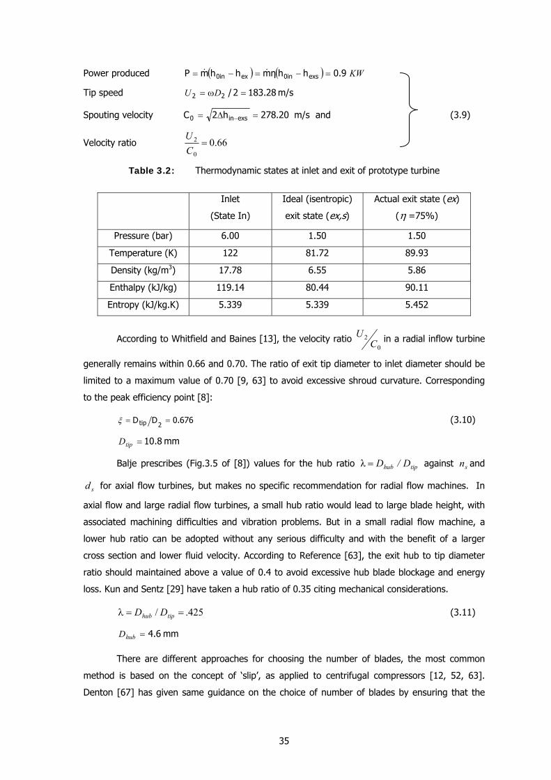
35

Power produced ( ) ( ) KW9.0hhηmhhmP exs0inex0in =−=−= &&

Tip speed 28.1832/22 =ω= DU m/s

Spouting velocity 20.278h2C exsin0 =Δ= − m/s and (3.9)

Velocity ratio 66.00

2 =CU

Table 3.2: Thermodynamic states at inlet and exit of prototype turbine

Inlet

(State In)

Ideal (isentropic)

exit state (ex,s)

Actual exit state (ex)

(η =75%)

Pressure (bar) 6.00 1.50 1.50

Temperature (K) 122 81.72 89.93

Density (kg/m3) 17.78 6.55 5.86

Enthalpy (kJ/kg) 119.14 80.44 90.11

Entropy (kJ/kg.K) 5.339 5.339 5.452

According to Whitfield and Baines [13], the velocity ratio 0

2C

U in a radial inflow turbine

generally remains within 0.66 and 0.70. The ratio of exit tip diameter to inlet diameter should be

limited to a maximum value of 0.70 [9, 63] to avoid excessive shroud curvature. Corresponding

to the peak efficiency point [8]:

676.0DD2tip ==ξ (3.10)

8.10=tipD mm

Balje prescribes (Fig.3.5 of [8]) values for the hub ratio tiphub D/D=λ against sn and

sd for axial flow turbines, but makes no specific recommendation for radial flow machines. In

axial flow and large radial flow turbines, a small hub ratio would lead to large blade height, with

associated machining difficulties and vibration problems. But in a small radial flow machine, a

lower hub ratio can be adopted without any serious difficulty and with the benefit of a larger

cross section and lower fluid velocity. According to Reference [63], the exit hub to tip diameter

ratio should maintained above a value of 0.4 to avoid excessive hub blade blockage and energy

loss. Kun and Sentz [29] have taken a hub ratio of 0.35 citing mechanical considerations.

425./ ==λ tiphub DD (3.11)

6.4=hubD mm

There are different approaches for choosing the number of blades, the most common

method is based on the concept of ‘slip’, as applied to centrifugal compressors [12, 52, 63].

Denton [67] has given same guidance on the choice of number of blades by ensuring that the

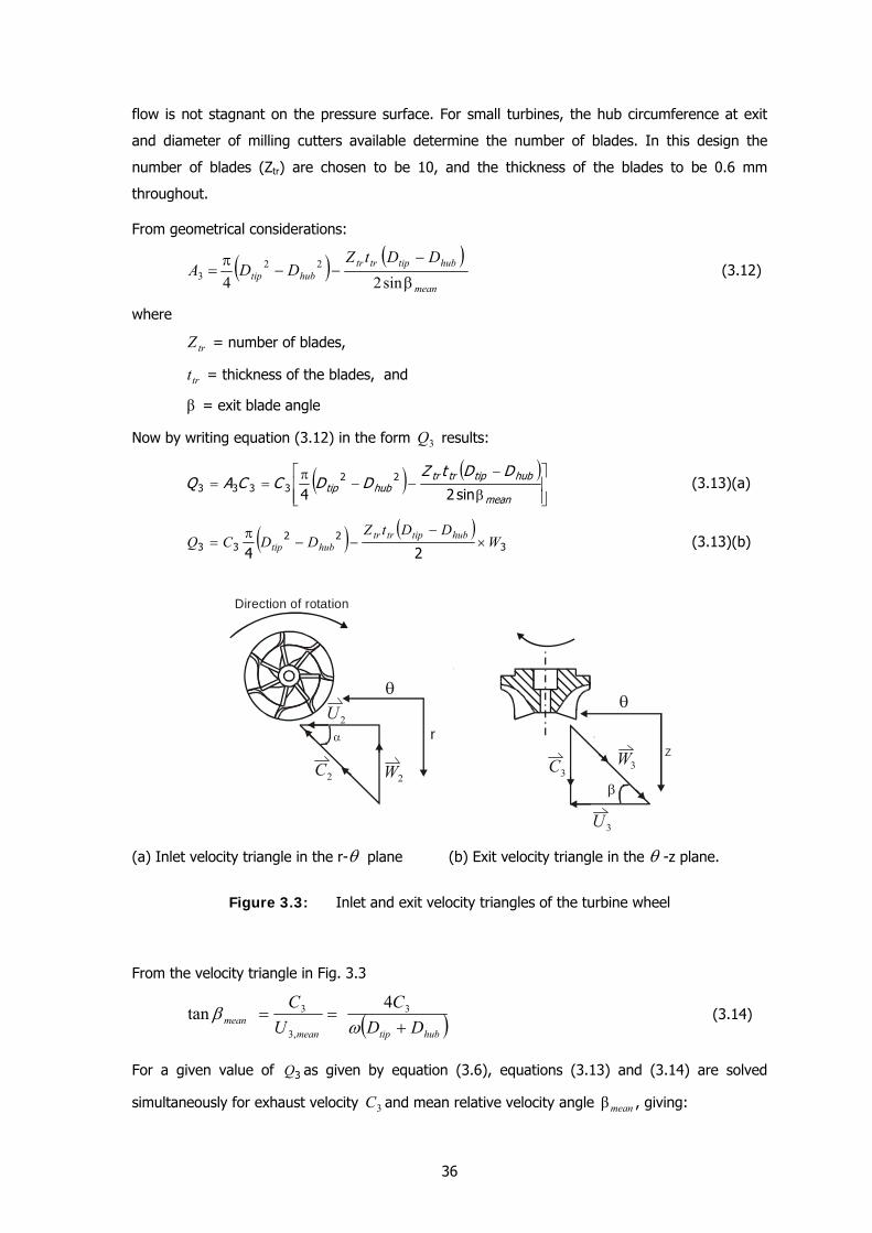
36

flow is not stagnant on the pressure surface. For small turbines, the hub circumference at exit

and diameter of milling cutters available determine the number of blades. In this design the

number of blades (Ztr) are chosen to be 10, and the thickness of the blades to be 0.6 mm

throughout.

From geometrical considerations:

( ) ( )mean

hubtiptrtrhubtip

DDtZDDA

β

−−−

π=

sin2422

3 (3.12)

where

trZ = number of blades,

trt = thickness of the blades, and

β = exit blade angle

Now by writing equation (3.12) in the form 3Q results:

( ) ( )⎥⎥⎦

⎤

⎢⎢⎣

⎡

β

−−−

π==

mean

hubtiptrtrhubtip

DDtZDDCCAQ

sin2422

3333 (3.13)(a)

( ) ( )3

2233 24

WDDtZ

DDCQ hubtiptrtrhubtip ×

−−−

π= (3.13)(b)

2U

2C 2W

θθ

3C 3W

3U

Direction of rotation

Zr

β

(a) Inlet velocity triangle in the r-θ plane (b) Exit velocity triangle in the θ -z plane.

Figure 3.3: Inlet and exit velocity triangles of the turbine wheel

From the velocity triangle in Fig. 3.3

( )hubtipmeanmean DD

CUC

+==

ωβ 3

,3

3 4tan (3.14)

For a given value of 3Q as given by equation (3.6), equations (3.13) and (3.14) are solved

simultaneously for exhaust velocity 3C and mean relative velocity angle meanβ , giving:

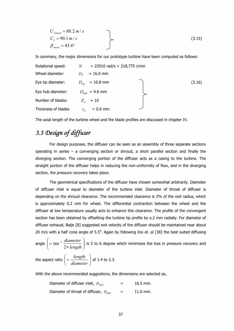
37

°==

=

6.45/1.90

/2.88

3

3

mean

mean

smCsmU

β (3.15)

In summary, the major dimensions for our prototype turbine have been computed as follows:

Rotational speed: N = 22910 rad/s = 218,775 r/min

Wheel diameter: 2D = 16.0 mm

Eye tip diameter: tipD = 10.8 mm (3.16)

Eye hub diameter: hubD = 4.6 mm

Number of blades: trZ = 10

Thickness of blades trt = 0.6 mm

The axial length of the turbine wheel and the blade profiles are discussed in chapter IV.

3.3 Design of diffuser

For design purposes, the diffuser can be seen as an assembly of three separate sections

operating in series – a converging section or shroud, a short parallel section and finally the

diverging section. The converging portion of the diffuser acts as a casing to the turbine. The

straight portion of the diffuser helps in reducing the non-uniformity of flow, and in the diverging

section, the pressure recovery takes place.

The geometrical specifications of the diffuser have chosen somewhat arbitrarily. Diameter

of diffuser inlet is equal to diameter of the turbine inlet. Diameter of throat of diffuser is

depending on the shroud clearance. The recommended clearance is 2% of the exit radius, which

is approximately 0.2 mm for wheel. The differential contraction between the wheel and the

diffuser at low temperature usually acts to enhance this clearance. The profile of the convergent

section has been obtained by offsetting the turbine tip profile by o.2 mm radially. For diameter of

diffuser exhaust, Balje [8] suggested exit velocity of the diffuser should be maintained near about

20 m/s with a half cone angle of 5.50. Again by following Ino et. al [38] the best suited diffusing

angle ⎟⎟⎠

⎞⎜⎜⎝

⎛∗

= −

lengthdiameter2

tan 1 is 5 to 6 degree which minimizes the loss in pressure recovery and

the aspect ratio ⎟⎠⎞

⎜⎝⎛=diameterlength

of 1.4 to 3.3.

With the above recommended suggestions, the dimensions are selected as,

Diameter of diffuser inlet, inDD = 16.5 mm.

Diameter of throat of diffuser, thDD = 11.0 mm.

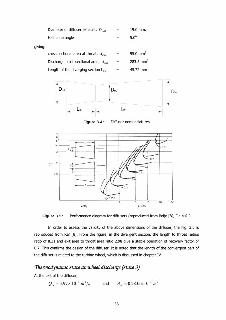
38

Diameter of diffuser exhaust, exDD = 19.0 mm.

Half cone angle = 5.00

giving:

cross sectional area at throat, thDA = 95.0 mm2

Discharge cross sectional area, thDA = 283.5 mm2

Length of the diverging section LdD = 45.72 mm

LcD LdD

DthD DexDDinD

Figure 3.4: Diffuser nomenclatures

Figure 3.5: Performance diagram for diffusers (reproduced from Balje [8], Fig 4.61)

In order to assess the validity of the above dimensions of the diffuser, the Fig. 3.5 is

reproduced from Ref [8]. From the figure, in the divergent section, the length to throat radius

ratio of 8.31 and exit area to throat area ratio 2.98 give a stable operation of recovery factor of

0.7. This confirms the design of the diffuser. It is noted that the length of the convergent part of

the diffuser is related to the turbine wheel, which is discussed in chapter IV.

Thermodynamic state at wheel discharge (state 3) At the exit of the diffuser,

smQex331097.3 −×= and 23102835.0 mAex

−×=

39

Therefore, exit velocity

sm0141028350

10973C 3

3

ex ...

AQ

ex

ex =××

== −

−

(3.17)

This velocity is below 20 m/s as suggested by Balje [8].

Exit stagnation enthalpy:

2C

hh2

exex0ex += (3.18)

kgkJ20.90102

1411.90 3

2

=×

+= .

Exit stagnation pressure:

pCρ21pp ex

2ex0ex ≈+= (because velocity exC is small) (3.19)

.505.1101486.5

215.1 5

2

bar=××+=

Neglecting losses in the diffuser, the stagnation enthalpy at turbine exit,

kgkJhh ex 20.90003 == , (3.20)

From the stagnation enthalpy, 03h , and stagnation pressure exp0 , the entropy 3s is estimated

[112] as

KkgkJs .452.53 =

And static enthalpy:

kgkJC

hh 15.86100021.9020.90

2

223

033 =×

−=−= (3.21)

From static enthalpy, kgkJh 15.863 = and KkgkJs .452.53 = , the density 3ρ calculated [167]

as 3ρ = 5.26 kg/m3.

The choice of =1k 1.11 is justified by comparing this density value with equations 3.6.

Therefore, the state point 3 is now fully described which can lead to the construction of velocity

triangle of the turbine.

Tip circumferential velocity

sm7.12310002

8.102291023 =

××== tip

tip

DU

ω (3.22)

Relative velocity at eye tip

23

23tip3tip CUW += (3.23)

sm153.090.1123.7 22 =+=

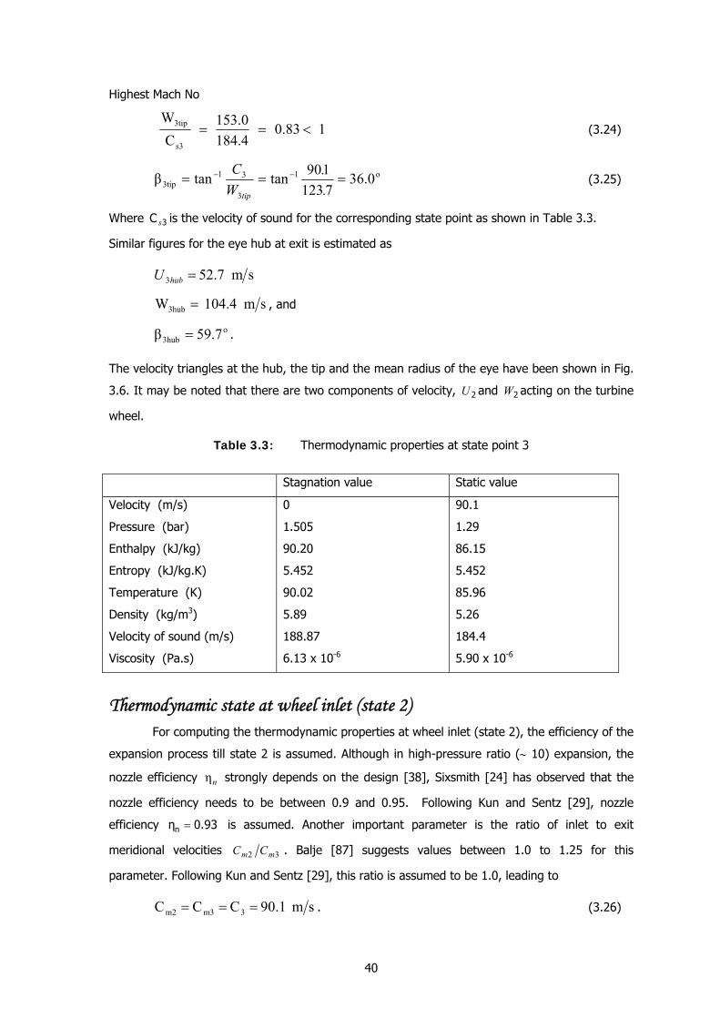
40

Highest Mach No

10.83184.4153.0

CW

s3

3tip <== (3.24)

o1

3

313tip 36.0

7123190tantanβ === −−

..

WC

tip

(3.25)

Where 3C s is the velocity of sound for the corresponding state point as shown in Table 3.3.

Similar figures for the eye hub at exit is estimated as

sm7.523 =hubU

sm104.4W3hub = , and

o3hub 59.7β = .

The velocity triangles at the hub, the tip and the mean radius of the eye have been shown in Fig.

3.6. It may be noted that there are two components of velocity, 2U and 2W acting on the turbine

wheel.

Table 3.3: Thermodynamic properties at state point 3

Stagnation value Static value

Velocity (m/s)

Pressure (bar)

Enthalpy (kJ/kg)

Entropy (kJ/kg.K)

Temperature (K)

Density (kg/m3)

Velocity of sound (m/s)

Viscosity (Pa.s)

0

1.505

90.20

5.452

90.02

5.89

188.87

6.13 x 10-6

90.1

1.29

86.15

5.452

85.96

5.26

184.4

5.90 x 10-6

Thermodynamic state at wheel inlet (state 2) For computing the thermodynamic properties at wheel inlet (state 2), the efficiency of the

expansion process till state 2 is assumed. Although in high-pressure ratio (∼ 10) expansion, the

nozzle efficiency nη strongly depends on the design [38], Sixsmith [24] has observed that the

nozzle efficiency needs to be between 0.9 and 0.95. Following Kun and Sentz [29], nozzle

efficiency =nη 0.93 is assumed. Another important parameter is the ratio of inlet to exit

meridional velocities 32 mm CC . Balje [87] suggests values between 1.0 to 1.25 for this

parameter. Following Kun and Sentz [29], this ratio is assumed to be 1.0, leading to

sm90.1CCC 3m3m2 === . (3.26)

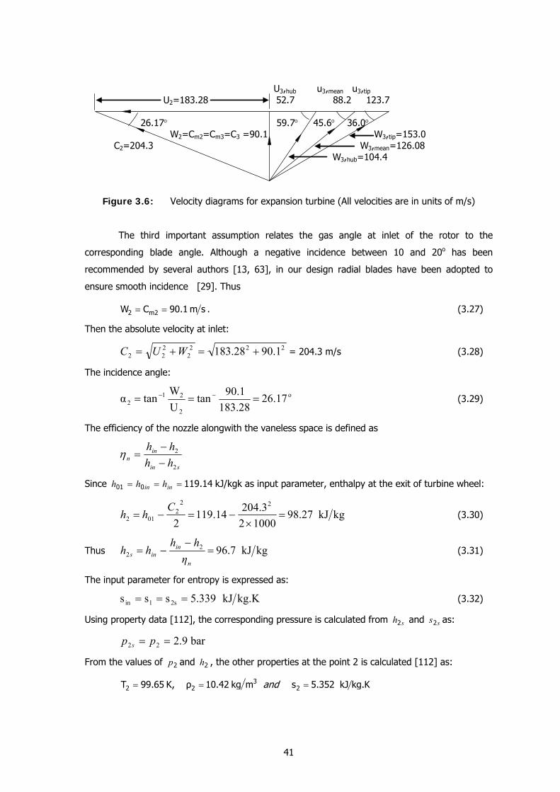
41

U3,hub u3,mean u3,tip U2=183.28 52.7 88.2 123.7 26.17° 59.7° 45.6° 36.0° W2=Cm2=Cm3=C3 =90.1 W3,tip=153.0 C2=204.3 W3,mean=126.08 W3,hub=104.4

Figure 3.6: Velocity diagrams for expansion turbine (All velocities are in units of m/s)

The third important assumption relates the gas angle at inlet of the rotor to the

corresponding blade angle. Although a negative incidence between 10 and 20o has been

recommended by several authors [13, 63], in our design radial blades have been adopted to

ensure smooth incidence [29]. Thus

= =2 m2W C 90.1 m s . (3.27)

Then the absolute velocity at inlet:

2222

222 1.9028.183 +=+= WUC = 204.3 m/s (3.28)

The incidence angle:

o

2

212 17.26

28.1831.90tan

UW

tanα === −− (3.29)

The efficiency of the nozzle alongwith the vaneless space is defined as

sin

inn hh

hh

2

2

−−

=η

Since 14.119001 === inin hhh kJ/kgk as input parameter, enthalpy at the exit of turbine wheel:

kgkJ98.2710002

204.3119.142

222

012 =×

−=−=C

hh (3.30)

Thus kgkJ96.722 =

−−=

n

inins η

hhhh (3.31)

The input parameter for entropy is expressed as:

kg.KkJ5.339sss 2s1in === (3.32)

Using property data [112], the corresponding pressure is calculated from sh2 and ss2 as:

bar2.922 == pp s

From the values of 2p and 2h , the other properties at the point 2 is calculated [112] as:

= = =32 2 2T 99.65 K, ρ 10.42 kg m s 5.352 kJ kg.Kand

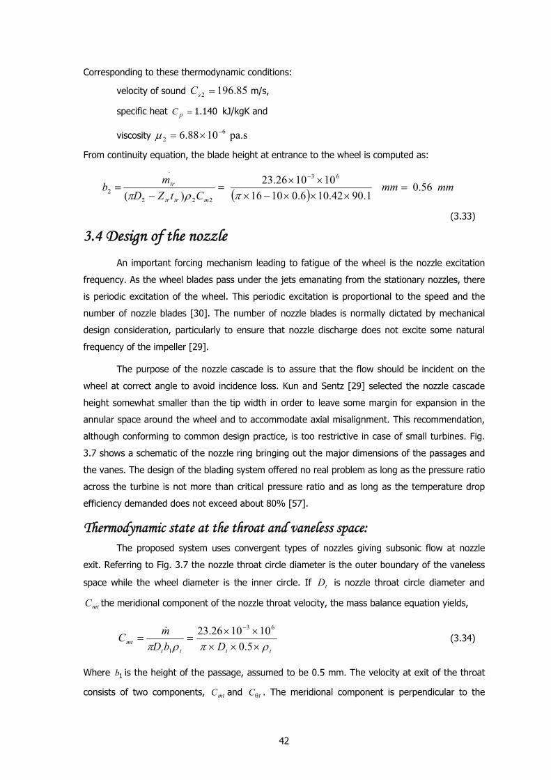
42

Corresponding to these thermodynamic conditions:

velocity of sound 85.1962 =sC m/s,

specific heat 140.1=pC kJ/kgK and

viscosity pa.s1088.6 62

−×=μ

From continuity equation, the blade height at entrance to the wheel is computed as:

222

.

2 )( mtrtr

tr

CtZDm

bρπ −

= ( ) mm1.9042.106.01016

101026.23 63

×××−×××

=−

πmm56.0=

(3.33)

3.4 Design of the nozzle

An important forcing mechanism leading to fatigue of the wheel is the nozzle excitation

frequency. As the wheel blades pass under the jets emanating from the stationary nozzles, there

is periodic excitation of the wheel. This periodic excitation is proportional to the speed and the

number of nozzle blades [30]. The number of nozzle blades is normally dictated by mechanical

design consideration, particularly to ensure that nozzle discharge does not excite some natural

frequency of the impeller [29].

The purpose of the nozzle cascade is to assure that the flow should be incident on the

wheel at correct angle to avoid incidence loss. Kun and Sentz [29] selected the nozzle cascade

height somewhat smaller than the tip width in order to leave some margin for expansion in the

annular space around the wheel and to accommodate axial misalignment. This recommendation,

although conforming to common design practice, is too restrictive in case of small turbines. Fig.

3.7 shows a schematic of the nozzle ring bringing out the major dimensions of the passages and

the vanes. The design of the blading system offered no real problem as long as the pressure ratio

across the turbine is not more than critical pressure ratio and as long as the temperature drop

efficiency demanded does not exceed about 80% [57].

Thermodynamic state at the throat and vaneless space: The proposed system uses convergent types of nozzles giving subsonic flow at nozzle

exit. Referring to Fig. 3.7 the nozzle throat circle diameter is the outer boundary of the vaneless

space while the wheel diameter is the inner circle. If tD is nozzle throat circle diameter and

mtC the meridional component of the nozzle throat velocity, the mass balance equation yields,

tttt

mt DbDmC

ρπρπ ×××××

==−

5.0101026.23 63

1

& (3.34)

Where 1b is the height of the passage, assumed to be 0.5 mm. The velocity at exit of the throat

consists of two components, mtC and tCθ . The meridional component is perpendicular to the

43

nozzle throat circle diameter, which determines the mass flow rate whereas the tCθ other

component is tangential to the throat.

Following Ref [29], mmDDt 28.17*08.1 2 == , leading to

t

mtCρ

93.856= (3.35)

Similar to the presence of two velocity components at the throat circle diameter, there

are two velocity components at the entry of the turbine wheel as shown in Fig. 3.3. From

conservation of angular momentum in free vortex flow over the vaneless space,

= =θt 2 2 tC U D D 183.28 1.08 sm.70169= (3.36)

Figure 3.7: Major dimensions of the nozzle and nozzle vane.

Thus,

22

222

2t

tCC

hh −+=

Since tC consists of two velocity components perpendicular to each other,

222

2222

2tmt

tCCC

hh θ−−+=

kgJC.. mt

22701691014119

223 −−×=

2

33

ρ10163671074104

t

.. ×−×= (3.37)

The relation between th and tρ given by equation (3.37) and the entropy conservation

relation given below [112] uniquely determines enthalpy and density at that throat. Assuming

isentropic expansion in the vaneless space,

kgKkJssst /352.521 ===

W t

D2

Vaneless SpaceDt

Dn

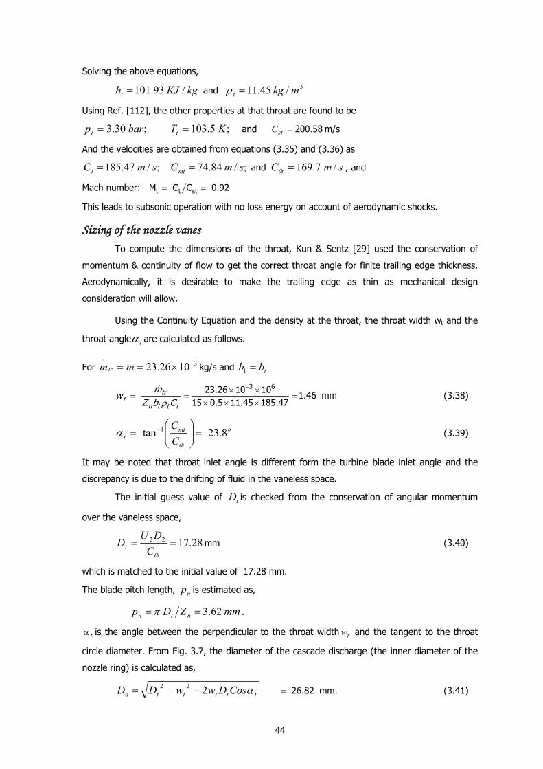
44

Solving the above equations,

kgKJht /93.101= and 3/45.11 mkgt =ρ

Using Ref. [112], the other properties at that throat are found to be

;5.103;30.3 KTbarp tt == and 58.200=stC m/s

And the velocities are obtained from equations (3.35) and (3.36) as

;/84.74;/47.185 smCsmC mtt == and smC t /7.169=θ , and

Mach number: = =t t stM C C 0.92

This leads to subsonic operation with no loss energy on account of aerodynamic shocks.

Sizing of the nozzle vanes To compute the dimensions of the throat, Kun & Sentz [29] used the conservation of

momentum & continuity of flow to get the correct throat angle for finite trailing edge thickness.

Aerodynamically, it is desirable to make the trailing edge as thin as mechanical design

consideration will allow.

Using the Continuity Equation and the density at the throat, the throat width wt and the

throat angle tα are calculated as follows.

For 3..

1026.23 −×== mmtr kg/s and tbb =1

ρ

−× ×= = =

× × ×

& 3 623.26 10 101.46 mm

15 0.5 11.45 185.47tr

tn t t t

mw

Z b C (3.38)

o

t

mtt C

C8.23tan 1 =⎟⎟

⎠

⎞⎜⎜⎝

⎛= −

θ

α (3.39)

It may be noted that throat inlet angle is different form the turbine blade inlet angle and the

discrepancy is due to the drifting of fluid in the vaneless space.

The initial guess value of tD is checked from the conservation of angular momentum

over the vaneless space,

28.1722 ==t

t CDUDθ

mm (3.40)

which is matched to the initial value of 17.28 mm.

The blade pitch length, np is estimated as,

mmZDp ntn 62.3==π .

tα is the angle between the perpendicular to the throat width tw and the tangent to the throat

circle diameter. From Fig. 3.7, the diameter of the cascade discharge (the inner diameter of the

nozzle ring) is calculated as,

tttttn CosDwwDD α222 −+= = 26.82 mm. (3.41)

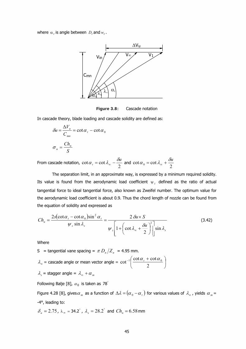
45

where tα is angle between tD and tw .

Figure 3.8: Cascade notation

In cascade theory, blade loading and cascade solidity are defined as:

0cotcot ααδ −=Δ

= tmn

u

CV

u

SChn

n =σ

From cascade notation, 2

cotcot ut

δλα −= ∞ and 2

cotcot 0uδλα += ∞

The separation limit, in an approximate way, is expressed by a minimum required solidity.

Its value is found from the aerodynamic load coefficient zψ defined as the ratio of actual

tangential force to ideal tangential force, also known as Zweifel number. The optimum value for

the aerodynamic load coefficient is about 0.9. Thus the chord length of nozzle can be found from

the equation of solidity and expressed as

( )

szsz

ttn

u

SusCh

λδλψ

δλψ

ααα

sin2

cot1

2sin

sincotcot22

20

⎥⎥⎦

⎤

⎢⎢⎣

⎡⎟⎠⎞

⎜⎝⎛ ++

×=

−=

∞

(3.42)

Where

S = tangential vane spacing = nn ZDπ = 4.95 mm.

∞λ = cascade angle or mean vector angle = ⎟⎠

⎞⎜⎝

⎛ +−

2cotcot

cot 01 αα t

sλ = stagger angle = mαλ +∞

Following Balje [8], 0α is taken as °78

Figure 4.28 [8], gives mα as a function of ( )tααλ −=Δ 0 for various values of ∞λ , yields mα =

-4°, leading to:

75.2=uδ , °∞ =λ 2.34 , °= 2.28sλ and 58.6=nCh mm

αt

α 0

C mn

λ∞λs

V inV∞ V1

ΔVu

46

3.5 Design of brake compressor

The shaft power generated by a turbine must be transferred to a braking device mounted

on the shaft. For relatively large amounts of power, an electrical generator [37, 77] is mostly

used as the braking device. A brake compressor is the most common choice for small

turboexpanders. The power generated by the turbine is used to drive a centrifugal compressor

which acts as a brake. In small turbine systems the energy is dissipated through a valve or orifice

in the brake circuit. The throttle valve is used to reduce the flow of gas through the compressor,

this reduces the load and consequently, there is a corresponding increase in speed. The

compressor should be over designed so that with the throttle fully open the turbine speed is less

than the designed value [76]. Thus, the turbine speed may be increased up to the designed value

by suitable adjustment of the throttle. Here a mixed flow centrifugal compressor is chosen which

uses same design principle as the turbine wheel. The efficiency of a brake compressor used as a

loading device does not influence the overall efficiency of the process plant [69].

Design inputs and basic dimensions The design inputs to the brake compressor are the following:

Process gas Air/ Nitrogen

Power to be dissipated (P) 0.9 kW (neglecting bearing friction losses)

Angular speed (ω) 22910.0 rad/s (2,18,775 r/min)

Inlet total pressure (p04) 1.12 bar

Inlet total temperature (T04) 300 K (ambient temperature)

Expected efficiency (ηb) 60 % [67]

To determine the compressor discharge pressure and flow rate, an estimate of the static

thermodynamic properties at the inlet (State 4) is needed.

11

204

211

−⎟⎠⎞

⎜⎝⎛ −+=

γγρρ

M

04

0494.0RTMp N= 18.1

30083142811200094.0

=×

××= kg/m3 (3.43)

for 044 94.0 ρρ =

Power dissipated b

sb hmP

η0Δ

=&

where sh0Δ is the total head across the isentropic compressor.

Also 4Q being the volume flow rate, the expression for power gives,

KWhQhm

b

s

b

sb 9.00440

.

=Δ

=Δ

ηρ

η

Substituting 60.0=bη and 18.14 =ρ kg/m3, the resultant expression is

47

9.45604 =Δ shQ Wm3/kg (3.44)

Ref. [8] gives the ns – ds diagram for a single stage centrifugal compressor. From this

diagram, the operating point is chosen in order to achieve proper velocity triangles within the

constraints of available power and rotational speed. Under these operating conditions,

,95.1=sn 9.2=sd (3.45)

sn and sd being defined as :

Specific speed

434

ss h

Qn

Δ=

ω

Specific diameter

4

415

QhD

d ss

Δ=

shΔ is the ideal static head across the compressor and 5D is the diameter of the impeller.

Balje [8] has pointed out that mixed flow geometry is necessary to obtain the highest efficiency

at these values of sn and sd . The design optimization is not required because the energy is

eventually dissipated. Thus a lower value of sn is chosen for radial blading.

Assuming zero swirl at inlet, [9],

WattUmP bsf 90025 == &φσ (3.47)

where, =φ power input factor 021.= [9]

sfσ = slip factor 78.05

5 ==UCθ [9]

5θC = Tangential component of the absolute velocity at exit

5U = peripheral speed at exit = 25Dω

Solving the equations (3.45) – (3.47) simultaneously with approximate value of 4ρ , we get:

m/s6.3122

kg/s0116.0

KJ/kg19.12/sm0098.0

,mm30.27

55

44

.

34

5

==

==

=Δ=

=

DU

Qm

hQ

D

b

s

ωρ

(3.48)

Substituting the value of 4Q in equation (3.44),

kgKJh s /10.410 =Δ

(3.46)

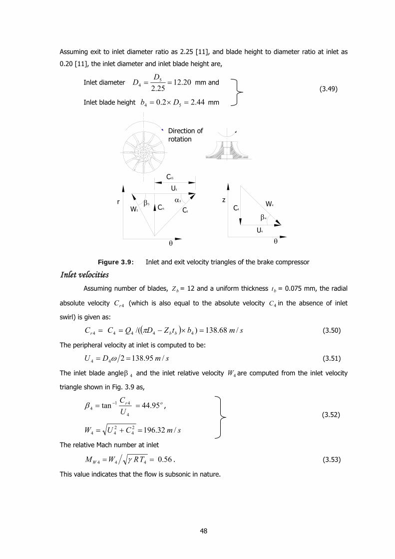
48

Assuming exit to inlet diameter ratio as 2.25 [11], and blade height to diameter ratio at inlet as

0.20 [11], the inlet diameter and inlet blade height are,

Inlet diameter 20.1225.25

4 ==D

D mm and

Inlet blade height 44.22.0 54 =×= Db mm

Direction of rotation

Cθ5

β4

β5α5

W5Cr5 C5

U5

r

θ θ

W4C4

U4

z

Figure 3.9: Inlet and exit velocity triangles of the brake compressor

Inlet velocities Assuming number of blades, bZ = 12 and a uniform thickness bt = 0.075 mm, the radial

absolute velocity 4rC (which is also equal to the absolute velocity 4C in the absence of inlet

swirl) is given as:

( ) smbtZDQCC bbr /68.138)/( 44444 =×−== π (3.50)

The peripheral velocity at inlet is computed to be:

smDU /95.138244 == ω (3.51)

The inlet blade angle 4β and the inlet relative velocity 4W are computed from the inlet velocity

triangle shown in Fig. 3.9 as,

or

UC

95.44tan4

414 == −β ,

smCUW /32.19624

244 =+=

The relative Mach number at inlet

56.0444 == TRWMW γ . (3.53)

This value indicates that the flow is subsonic in nature.

(3.49)

(3.52)

49

Number of blades Unlike the turbine wheel, the output of the brake compressor is eventually dissipated in a

valve, particularly in small machines. Therefore, it is not necessary to have efficient blade

geometry in the impeller. There are several empirical relations for determining the optimum

number of blades. Well known among them are [11]:

Eck: 1

5

45 )1(sin5.8 −−=

DD

zb β

Pfleirderer: ⎟⎠

⎞⎜⎝

⎛ +⎟⎟⎠

⎞⎜⎜⎝

⎛−+

=2

sin5.6 54

45

54 ββDDDD

zb

Stepanoff: 531 β=bz with 5β given in degrees.

The formulas give 17, 16 and 18 blades respectively for the impeller. A choice of number of

blades of 12 and thickness of 0.75 mm are justified from the present design point of view.

Thermodynamic variables at inlet and exit Static temperature at inlet:

KCC

TTp

76.2902

24

044 =−= (3.55)

Inlet static pressure:

004.11

04

4044 =⎟⎟

⎠

⎞⎜⎜⎝

⎛=

−γγ

TT

pp bar, (3.56)

γ being the specific heat ratio 1.41. The density at inlet is calculated as

16.14

44 ==

RTp

ρ kg/m3 (3.57)

This is close to the assumed value of 1.18 kg/m3.

The rise in stagnation temperature through the compressor can be obtained from the

power expended and the mass flow rate through the compressor. Thus

7.3741041*0116.0

9003000405 =+=+=pbCm

PTT&

K (3.58)

The exit stagnation temperature for an isentropic compressor with isentropic efficiency, 6.0=ηb

is estimated as,

82.3440405 =+=pb

bs Cm

PTT

&

ηK (3.59)

The corresponding stagnation pressure is found to be:

(3.54)

50

82.11

04

050405 =⎟⎟

⎠

⎞⎜⎜⎝

⎛=

−γγ

TTpp s bar (3.60)

Exit velocities The absolute exit velocity:

( ) smhhC ss /55.2622 5055 =−= (3.61)

Using the value of 0.82 for the slip factor, the tangential velocity:

smUC /85.24382.0 55 ==θ

smCCCr /3.9725

255 =−= θ

The exit blade angle:

θ

β − ⎛ ⎞= =⎜ ⎟⎜ ⎟−⎝ ⎠

1 55

5 5tan 54.74orC

U C

and the absolute exit angle :

or

CC

75.21tan5

515 =⎟⎟

⎠

⎞⎜⎜⎝

⎛= −

θ

α

The relative velocity at exit:

smecCW r /15.119cos 555 == β (3.64)

Exit temperature KCh

TTp

adst 71.311045 =Δ

+=

and exit pressure: barTT

pp 28.11

04

5045 =⎟⎟

⎠

⎞⎜⎜⎝

⎛=

−γγ

Density at exit: 3

5

55 /38.1 mkg

RTp

==ρ

The required blade height at exit:

( ) 5555

rbb

b

CtZDm

bρ−π

=&

= 1.12 mm (3.66)

3.6 Design of shaft

Because the strength of most materials improves at low temperature, the general

perception among engineers and scientists is that stress considerations are unimportant in case

of cryogenic turbines. In reality, cryogenic turbines, because of the moderate to high-pressure

ratio and low flow rates operate at high rotational speeds, leading to significant centrifugal

stresses in the shaft. The shaft transmits the torque produced by the turbine to the brake

(3.62)

(3.63)

(3.65)

51

compressor. Torsional shear stress is not dominant due to the high rotational speed and small

power transmission. Also the turboexpander is vertically oriented and bending load is neglected

due to the absence of any radial load. Important considerations in the design of the shaft are:

• number and size of components linked with the shaft,

• tangential speed on bearing surfaces,

• stress at the root of the collar,

• critical speed in shaft bending mode,

• heat conduction between the warm and the cold ends and

• overall compactness of the system.

The major dimensions of the shaft include:

• diameter of the shaft,

• diameter of the collar and

• length of the shaft

Sixsmith and Swift [113] suggest that shafts should be designed on the basis of safe

critical speed and checked for heat conduction. In our approach, however, the dimensions have

been chosen based on data from comparable installations by other workers and these data have

been verified for maximum stress, critical speed and heat conduction. Ino et. al [38] have

chosen a shaft diameter of 16 mm for their helium turbine rotating at 2,30,000 r/min, while

Yang et al [33] have chosen 18 mm for their air turbine rotating at 180,000 r/min. A shaft of

diameter 16 mm and length 88.1 mm with a thrust collar of diameter 30 mm has been selected in

the present case. Detailed drawing of the shaft is given in Fig. A3.

Kun and Sentz [29] have suggested that it is necessary to perform detailed stress

analysis when the operating surface speed of the turbine or compressor wheel exceeds about

50% of the critical speed at which the material starts yielding in a simple disk of same diameter

rotating at the same speed.

The peripheral speed on the shaft surface is computed to be:

ω= = =2 22910.0 * 0.016 2 183.28surfV d m/s. (3.67)

and that on the tip of the collar is 343.65 m/s.

A preliminary calculation considering the collar as a solid disk gives [114]

σ ρ= = × × =2 21 18000 343.65 314.92

3 3ss surfV MPa (3.68)

This value is more than recommended design stress of 230 MPa for stainless steel SS 304

[1], justifying the need for other material. Hence K-Monel-500 for the shaft material is chosen

having design stress of 790 Mpa. By using K-Monel-500 as a shaft material the possibility of

yielding of the shaft is very less.

52

Shaft speed is generally limited by the first critical speed in bending. This limitation for a

given diameter determines the shaft length. The overhang distance into the cold end, strongly

affects the conductive heat leak penalty to the cold end [31].

The first bending critical speed for a uniform shaft is given by the formula [113]

( )ρEldf 29.0= Hz (3.69)

where d is the diameter of the shaft, l is the length, E is the Young’s modulus and ρ is the

density of the material. Considering the shaft to be a K-Monel-500 cylinder of diameter 16.0 mm

and length 88.1 mm, the bending critical speed is

×⎛ ⎞= = =⎜ ⎟⎝ ⎠

10

2

0.016 18 100.9 8544 Hz 5,12,640

84400.0881f r/min

This is well above the operating speed of 2,18,775 r/min.

The gas lubricated bearings of a cryogenic turbine need to be maintained at room

temperature to get the necessary viscosity. This requires a strong temperature gradient over the

shaft overhang between the lower journal bearing and the turbine wheel. The rate of heat flow

can be reduced by (a) using material of lower thermal conductivity (b) reducing the shaft

diameter below the lower journal bearing and (c) by using a hollow shaft in that section.

The principal features of the shaft

A collar alongwith the thrust plates anchored to the housing, acts as a pair of thrust

bearings.

A step at the top end of the shaft provides a seat for the brake compressor [Fig. A3].

A step at the bottom end of the shaft, providing a seat for the turbine wheel.

A hollow section at the bottom end of the shaft to reduce the heat transfer rate from

the warm to the cold end.

3.7 Design of vaneless space The discharge air at the nozzle exit reaches the impeller after passing through vaneless

space. As this space is located just adjacent to the impeller, its configuration seems to influence

the condition of inflow to the impeller. Watanabe [72] pointed out that too small a radial

clearance causes reduction in efficiencies and at large radial clearances performance

characteristics of turbine are less influenced by the clearances, and in addition, that an optimum

radial clearance ought to exist. Irregularities of nozzle discharge flow to the impeller entry can be

reduced at larger clearance obtaining the maximum efficiency. But the friction losses within the

vaneless space will increase at large clearance giving less efficiency. Thus, inflow irregularities

and friction losses should be taken into consideration in order to estimate the optimum radial

53

clearance between nozzle vanes and the impellers. By following the reference [72] the flow path

length of fluid is expressed as follows

α

εsin

S rvs =

where,

=rε radial clearance between the nozzle and turbine impeller

=α flow angle at nozzle exit

3.8 Selection of bearings

Successful development of a turboexpander strongly depends on the performance of the

bearings and their protection systems. In this system gas-lubricated bearings, the aerostatic

thrust bearings and the aerodynamic tilting pad journal bearings are employed. The main

advantages of these bearings are high stability to self-excitation, external dynamic load and fewer

constraints on fabrication, albeit at the cost of some process gas consumption [115]. The radial

load arises primarily due to rotor imbalance and is taken up by a pair of aerodynamic journal

bearing. Apart from imbalance load, the journal bearings ensure shaft alignment. Thrust bearing

supports the thrust load comprises of the rotor weight and the difference of force due to pressure

between the turbine and the compressor ends.

(i) Aerostatic thrust bearing Aerostatic thrust bearings have come up as a reliable solution for supporting high-speed

rotors, especially for cases where the use of oil bearings is discouraged. This is particularly true

for cryogenic turboexpander where use of oil is avoided due to the possibility of seepage and

contamination of the process gas. On the other hand, aerostatic thrust bearing, owing to their

high load carrying capacity and reliability have remained largely unchanged. Although in most

cases the thrust load is unidirectional, that’s why a double thrust bearing is always provided as a

stop in case of accidental thrust reversal. The shaft is vertically oriented and runs at high speed.

By following the procedure of Chakraborty [84], the double thrust bearing has been

designed assuming an eccentricity ratio of 0.1, supply pressure of 6.0 bar and discharged

pressure of 1.5 bar. Based on the relevant data from literature, the following parameters have

been computed.

Feed hole or orifice diameter d0 = 0.4 mm

Outer radius of bearing rt1 = 15 mm

Inner radius of the bearing rt2 = 8.5 mm

Feed hole pitch circle rt0 = 11.75 mm

Number of feed orifices nh = 8

Bearing clearance hbg = 12 μm

54

The bearing outer diameter is kept equal to that of the shaft collar. The shaft diameter

determines the inner diameter of the bearing with a radial clearance of 1mm between the shaft

and the thrust plates. The feed hole pitch circle diameter is chosen from the consideration of

equal inward and outward flow of bearing gas. Available drill bit sizes influence the choice of feed

hole diameter. The diameters of the orifices in the upper and the lower thrust plates are

computed to match the load capacity while keeping the gas flow at the minimum.

A pair of thrust plates and the shaft collar form the double thrust bearing. Apart from the

feed hole or orifice larger holes on the outer side on the bearing are provided for connecting the

high pressure gas line. One O-ring is used to ensure the entry of high pressure in the outer large

holes.

(ii) Pivot-less tilting pad gas journal bearing

A pivot-less tilting pad bearing consists of three pads floating around the journal, within

the pad housing, surrounded by gas films on all sides. The three pads and the shaft form the

journal bearing system is shown in Fig. A6. Each pad basically consists of a front face that forms

the bearing surface, a back face, a network of three holes. High pressure from the bearing

surface is communicated to the back face of the pad through the holes. This generates a

pressure profile at the back face. The forces coming into picture are the aerodynamic load on the

pad, the frictional force on the bearing surface and the force due to pressure distribution at the

pad back face. The normal forces developed in the bearing clearance and at the back face, along

with the frictional force due to rotor motion, determine the equilibrium pad tilt. This type of tilting

pad bearings is specially suited for supporting small rotors.

By following the procedure of Chakraborty [84] the tilting pad bearing has been designed

with the basic input parameters like bearing gas, ambient conditions, rotor geometry and

rotational speed. The mean radial clearance is kept quite large, keeping in view of the machining

difficulties. This clearance is however much less than the radial clearance provided between the

turbine and its diffuser as well as that between the brake compressor and its casing, to prevent

rubbing at high speeds. The designed clearance of 10μm between the pad back face and housing

is also achievable. The pad length is decided from consideration of available axial space; which is

taken as L/D =1. A 3-pad geometry with a span of 120° for each pad is chosen. The bleed and

connecting holes should be large, to communicate the pressure generated at the bearing

clearance to the back face of the pad without any significant pressure drop; too large a hole

would starve the bearing. It has been chosen a diameter of 1.75 mm for the bleed holes and 1.3

mm for the connecting holes. Care has been taken for rotor eccentricity such that a pad

equilibrium solution is possible.

55

3.9 Supporting structure Bearing housing

The bearing housing is the central component providing support to the two journal

bearings and the two thrust bearings. It is one of the most intricate components in the whole

assembly, not because of any requirement of high precision, but due to the sheer number and

variety of features. In other words, the bearing housing element provides both a structural

stability and thermal isolation between the warm end and cold end of the machine. The main

features of the housing design can be listed as follows:

A groove is provided to accommodate the two tilting pad journal bearings and two thrust

bearings.

A radial hole is drilled in the center of the shaft collar for accommodating the high

pressure supply lines and the low pressure exhaust lines to and from the thrust bearings

and for the proximity probe assembly.

Two lock nuts are provided, one in turbine side and another on compressor side to set all

the bearings and insulator inside the housing.

Flanges are provided at the top and bottom end of the housing to attach the warm end

casing and cold end casing.

An important function of the bearing housing is to provide thermal isolation between the

warm and the cold ends. The wall thickness is reduced wherever possible to meet this

objective.

Apart from the bearings, the housing also supports the labyrinth seal, speed and

vibrations sensors. Detailed drawings of the bearing housing are given in Figs in Appendix.

The Cap Base

The cap base between the two thrust plates is one of the most vital components of the

turbine. The cap base acting as thrust spacer has a two-fold function. It acts as distance pieces,

adjusting the clearances between parts and fixing tolerances where appropriate. They also make

way for the exhaust gas leaving the thrust bearings to flow to the outside. The thickness of this

spacer exceeds that of the shaft collar by the required amount of clearance. Through a radial hole

machined on its groove, this cap base also allows the exhaust bearing gas from the inner edges

of the thrust bearings to flow out. It also connects to proximity sensor to measure the rotational

speed.

Seal Heat inleak may occur from any of these sources.

• The environment

56

• Heat generated within the machine

• Heat carried into the machine by the lubricant

Heat entering the cold area does so mainly by conduction along the structural parts of the

machine, but some may enter by convection. The machine is usually supported by the part of its

structure which is at the highest temperature, and the flow paths to the cold end being made as

resistant to heat flow as possible by the use of minimum cross sectional areas consistent with

strength. Materials having low thermal conductivity are used and heat insulating materials are

incorporated wherever possible. Gas seals are used to limit the leakage of process gas along the

shaft or across a fully shrouded wheel. They also provide a means of adjusting the axial forces

acting on the rotor in that they are used to define the areas over which high or low pressure acts.

The most usual form of gas seal is the labyrinth. For a given pressure differential the leakage flow

will be lower than for a plain seal of equal diametrical clearance.

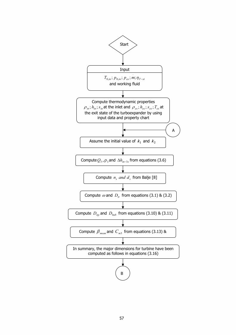
57

Start

Input

stTexinin mppT −η;;;;.

,0,0

and working fluid

A

Assume the initial value of 1k and 2k

Compute 3Q , 3ρ and sinh 3−Δ from equations (3.6)

Compute thermodynamic properties

ininin sh ;;ρ at the inlet and exexexex Tsh ;;;ρ at the exit state of the turboexpander by using

input data and property chart

Compute ss dandn from Balje [8]

Compute ω and trD from equations (3.1) & (3.2)

Compute tipD and hubD from equations (3.10) & (3.11)

Compute meanβ and 3mC from equations (3.13) &

In summary, the major dimensions for turbine have been computed as follows in equations (3.16)

B

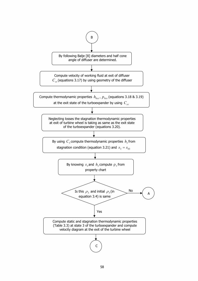
58

Compute thermodynamic properties exex ph 00 , (equations 3.18 & 3.19)

at the exit state of the turboexpander by using exC

By using 3C compute thermodynamic properties 3h from

stagnation condition (equation 3.21) and 033 ss =

Compute velocity of working fluid at exit of diffuser

exC (equations 3.17) by using geometry of the diffuser

By following Balje [8] diameters and half cone angle of diffuser are determined.

B

Neglecting losses the stagnation thermodynamic properties at exit of turbine wheel is taking as same as the exit state

of the turboexpander (equations 3.20).

By knowing 3s and 3h compute 3ρ from

property chart

A Is this 3ρ and initial 3ρ (in

equation 3.4) is same

Yes

No

Compute static and stagnation thermodynamic properties (Table 3.3) at state 3 of the turboexpander and compute

velocity diagram at the exit of the turbine wheel

C

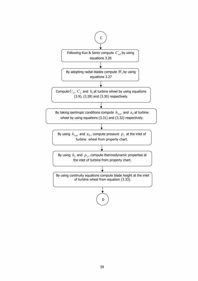
59

Following Kun & Sentz compute 2mC by using

equations 3.26

C

By adopting radial blades compute 2W by using equations 3.27

Compute 2U , 2C and 2h at turbine wheel by using equations (3.9), (3.28) and (3.30) respectively.

By taking isentropic conditions compute adh2 and 2s at turbine

wheel by using equations (3.31) and (3.32) respectively.

By using adh2 and 2s , compute pressure 2p at the inlet of

turbine wheel from property chart.

By using 2h and 2p , compute thermodynamic properties at the inlet of turbine from property chart.

By using continuity equations compute blade height at the inlet of turbine wheel from equation (3.33).

D

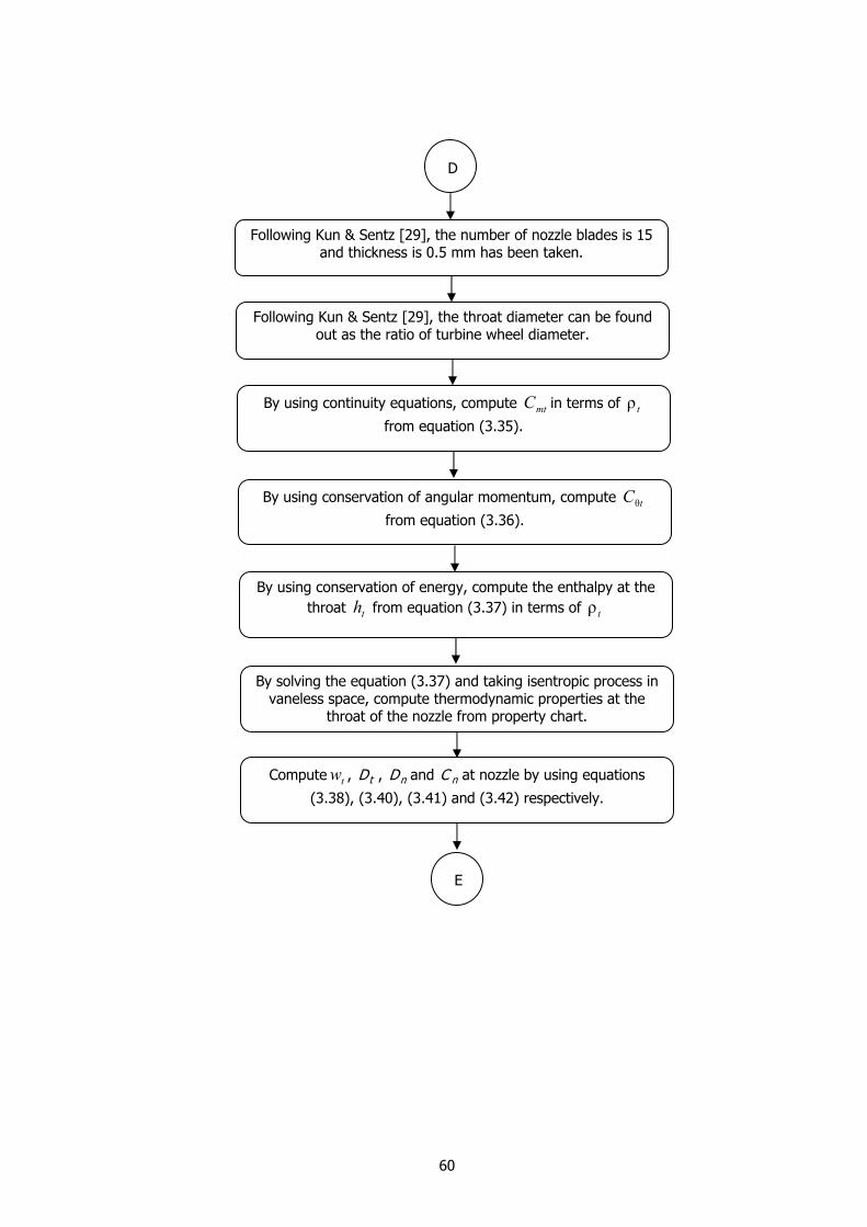
60

D

Following Kun & Sentz [29], the number of nozzle blades is 15 and thickness is 0.5 mm has been taken.

Following Kun & Sentz [29], the throat diameter can be found out as the ratio of turbine wheel diameter.

By using continuity equations, compute mtC in terms of tρ

from equation (3.35).

By using conservation of angular momentum, compute tCθ

from equation (3.36).

By using conservation of energy, compute the enthalpy at the throat th from equation (3.37) in terms of tρ

By solving the equation (3.37) and taking isentropic process in vaneless space, compute thermodynamic properties at the

throat of the nozzle from property chart.

Compute tw , tD , nD and nC at nozzle by using equations

(3.38), (3.40), (3.41) and (3.42) respectively.

E

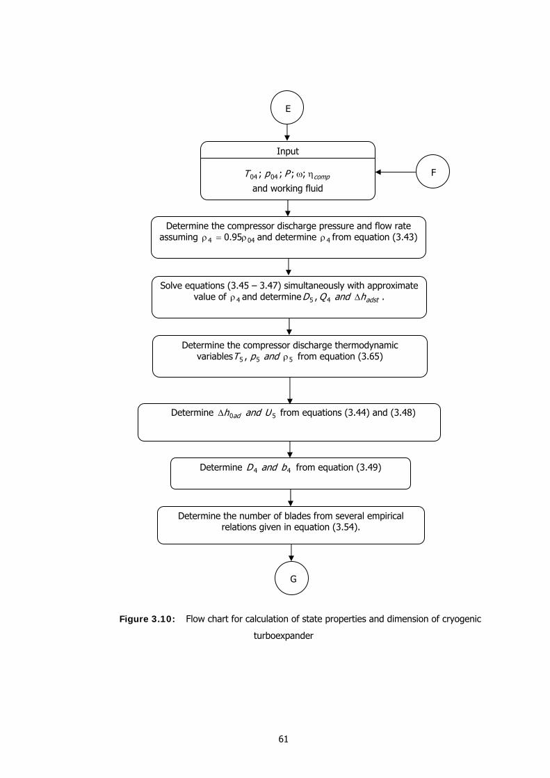
61

Figure 3.10: Flow chart for calculation of state properties and dimension of cryogenic

turboexpander

E

Input

compPpT ηω;;;; 0404

and working fluid

Determine the compressor discharge pressure and flow rate assuming 044 95.0 ρ=ρ and determine 4ρ from equation (3.43)

Solve equations (3.45 – 3.47) simultaneously with approximate value of 4ρ and determine adsthandQD Δ45 , .

Determine the compressor discharge thermodynamic variables 555 , ρandpT from equation (3.65)

F

Determine 50 Uandh adΔ from equations (3.44) and (3.48)

Determine 44 bandD from equation (3.49)

Determine the number of blades from several empirical relations given in equation (3.54).

G

Chapter 4

Determination of Blade Profile

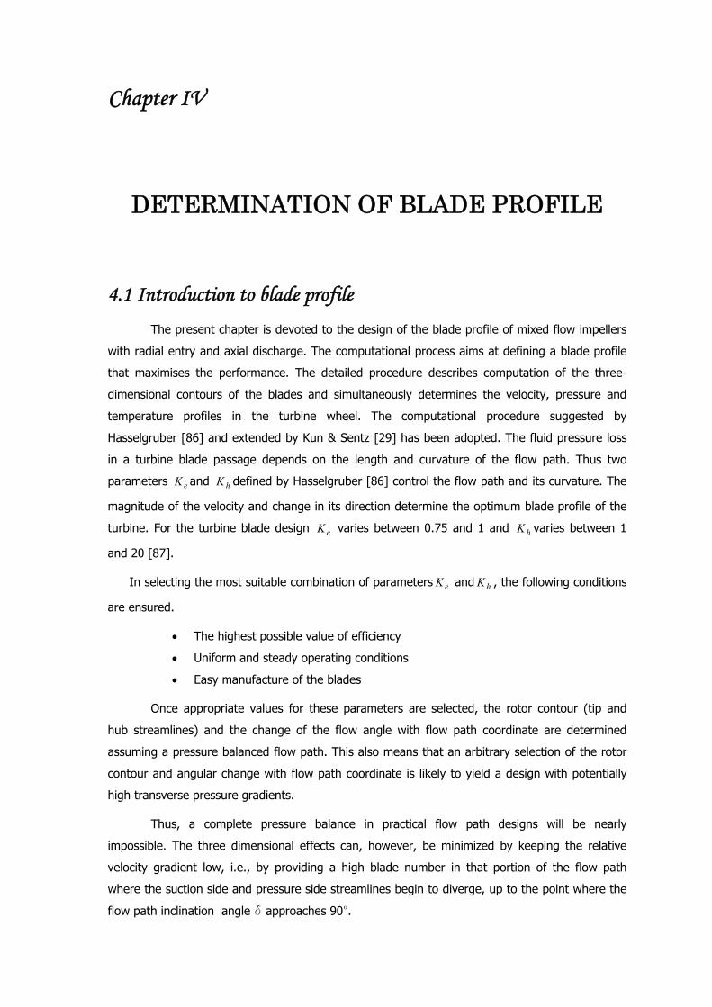
Chapter IV

DETERMINATION OF BLADE PROFILE

4.1 Introduction to blade profile The present chapter is devoted to the design of the blade profile of mixed flow impellers

with radial entry and axial discharge. The computational process aims at defining a blade profile

that maximises the performance. The detailed procedure describes computation of the three-

dimensional contours of the blades and simultaneously determines the velocity, pressure and

temperature profiles in the turbine wheel. The computational procedure suggested by

Hasselgruber [86] and extended by Kun & Sentz [29] has been adopted. The fluid pressure loss

in a turbine blade passage depends on the length and curvature of the flow path. Thus two

parameters eK and hK defined by Hasselgruber [86] control the flow path and its curvature. The

magnitude of the velocity and change in its direction determine the optimum blade profile of the

turbine. For the turbine blade design eK varies between 0.75 and 1 and hK varies between 1

and 20 [87].

In selecting the most suitable combination of parameters eK and hK , the following conditions

are ensured.

• The highest possible value of efficiency

• Uniform and steady operating conditions

• Easy manufacture of the blades

Once appropriate values for these parameters are selected, the rotor contour (tip and

hub streamlines) and the change of the flow angle with flow path coordinate are determined

assuming a pressure balanced flow path. This also means that an arbitrary selection of the rotor

contour and angular change with flow path coordinate is likely to yield a design with potentially

high transverse pressure gradients.

Thus, a complete pressure balance in practical flow path designs will be nearly

impossible. The three dimensional effects can, however, be minimized by keeping the relative

velocity gradient low, i.e., by providing a high blade number in that portion of the flow path

where the suction side and pressure side streamlines begin to diverge, up to the point where the

flow path inclination angle δ approaches 90°.

63

The design of blade profile is carried out by Hasselgruber’s approach [86]. The equations

are derived in a body fitted orthogonal coordinate system (t, b, n). The coordinate t is the

direction along the central streamline, the coordinate b is the lateral coordinate between the

suction and the pressure surfaces and the coordinate n refers to depth of the flow path in the

turbine passage. The author also defines the meridional coordinate s to correlate the body fitted

coordinate system with the cylindrical coordinate system (r, θ, z) where the s coordinate lies on

the r-z plane. Figures 4.1 and 4.2 show the flow velocity and coordinate transformation

respectively.

W2

ω

U2

C2

r2

r3W3

C3

C

U

U3

WCM

Detail A

α β

WC CM=WM

Uα2

β3

Inlet of Turbine Wheel (State 2)

Outlet of Turbine Wheel (State 3)

W3

C3

U3

β3

Detail B

Detail B

Detail A

t s

Figure 4.1: Illustration of flows in radial axial impeller

π/2-βδ

ω

r δ

π/2-βθ(u)

r

s(Cm)

z

n

b

t(W)

Figure 4.2: Coordinate system

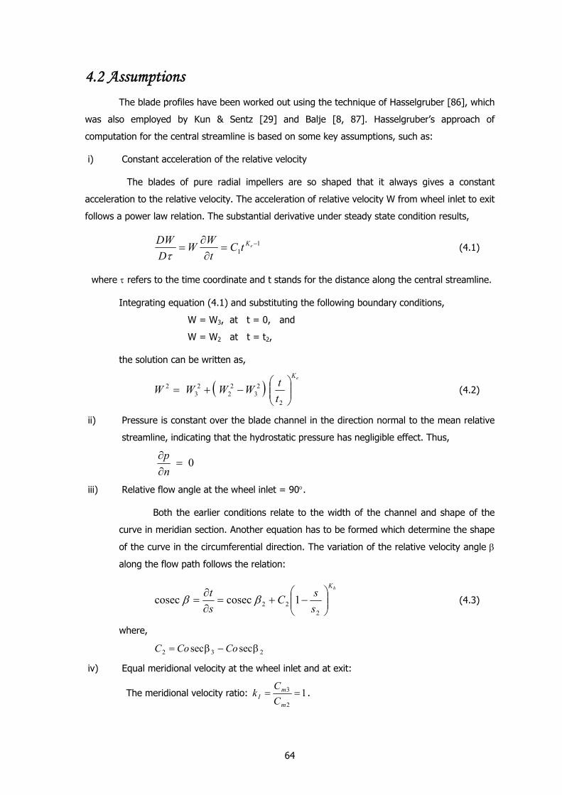
64

4.2 Assumptions The blade profiles have been worked out using the technique of Hasselgruber [86], which

was also employed by Kun & Sentz [29] and Balje [8, 87]. Hasselgruber’s approach of

computation for the central streamline is based on some key assumptions, such as:

i) Constant acceleration of the relative velocity

The blades of pure radial impellers are so shaped that it always gives a constant

acceleration to the relative velocity. The acceleration of relative velocity W from wheel inlet to exit

follows a power law relation. The substantial derivative under steady state condition results,

11

−=∂∂

= eKtCtWW

DDWτ

(4.1)

where τ refers to the time coordinate and t stands for the distance along the central streamline.

Integrating equation (4.1) and substituting the following boundary conditions,

W = W3, at t = 0, and

W = W2 at t = t2,

the solution can be written as,

( )eK

ttWWWW ⎟⎟⎠

⎞⎜⎜⎝

⎛−+=

2

23

22

23

2 (4.2)

ii) Pressure is constant over the blade channel in the direction normal to the mean relative

streamline, indicating that the hydrostatic pressure has negligible effect. Thus,

0=∂∂np

iii) Relative flow angle at the wheel inlet = 90°.

Both the earlier conditions relate to the width of the channel and shape of the

curve in meridian section. Another equation has to be formed which determine the shape

of the curve in the circumferential direction. The variation of the relative velocity angle β

along the flow path follows the relation:

hK

ssC

st

⎟⎟⎠

⎞⎜⎜⎝

⎛−+=

∂∂

=2

22 1coseccosec ββ (4.3)

where,

232 secsec β−β= CoCoC

iv) Equal meridional velocity at the wheel inlet and at exit:

The meridional velocity ratio: 12

3 ==m

mI CC

k .

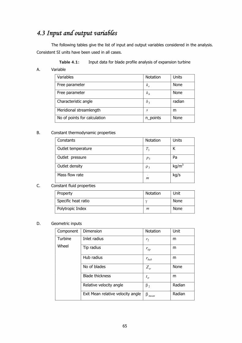
65

4.3 Input and output variables

The following tables give the list of input and output variables considered in the analysis.

Consistent SI units have been used in all cases.

Table 4.1: Input data for blade profile analysis of expansion turbine

A. Variable

Variables Notation Units

Free parameter ek None

Free parameter hk None

Characteristic angle 3δ radian

Meridional streamlength s m

No of points for calculation n_points None

B. Constant thermodynamic properties

Constants Notation Units

Outlet temperature 3T K

Outlet pressure 3p Pa

Outlet density 3ρ kg/m3

Mass flow rate .m

kg/s

C. Constant fluid properties

Property Notation Unit

Specific heat ratio γ None

Polytropic Index m None

D. Geometric inputs

Component Dimension Notation Unit

Inlet radius 2r m

Tip radius tipr m

Hub radius hubr m

No of blades trZ None

Blade thickness trt m

Relative velocity angle 2β Radian

Turbine

Wheel

Exit Mean relative velocity angle meanβ Radian

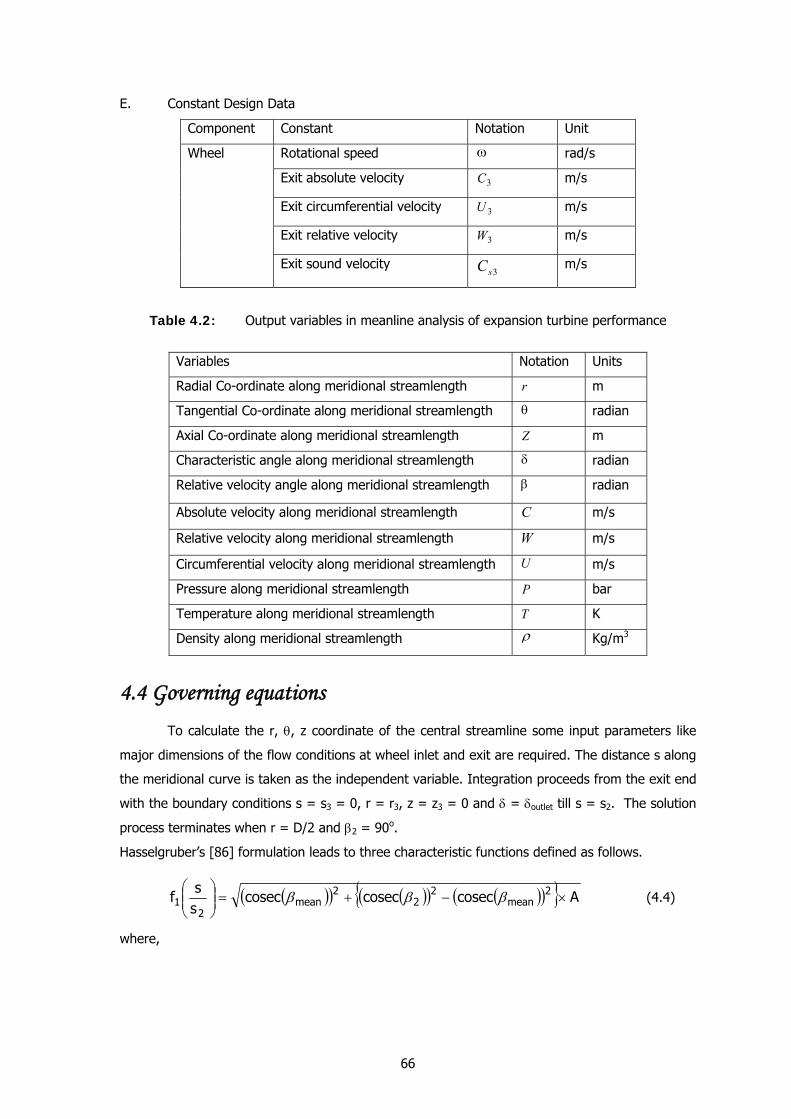
66

E. Constant Design Data

Component Constant Notation Unit

Rotational speed ω rad/s

Exit absolute velocity 3C m/s

Exit circumferential velocity 3U m/s

Exit relative velocity 3W m/s

Wheel

Exit sound velocity 3sC m/s

Table 4.2: Output variables in meanline analysis of expansion turbine performance

Variables Notation Units

Radial Co-ordinate along meridional streamlength r m

Tangential Co-ordinate along meridional streamlength θ radian

Axial Co-ordinate along meridional streamlength Z m

Characteristic angle along meridional streamlength δ radian

Relative velocity angle along meridional streamlength β radian

Absolute velocity along meridional streamlength C m/s

Relative velocity along meridional streamlength W m/s

Circumferential velocity along meridional streamlength U m/s

Pressure along meridional streamlength P bar

Temperature along meridional streamlength T K

Density along meridional streamlength ρ Kg/m3

4.4 Governing equations

To calculate the r, θ, z coordinate of the central streamline some input parameters like

major dimensions of the flow conditions at wheel inlet and exit are required. The distance s along

the meridional curve is taken as the independent variable. Integration proceeds from the exit end

with the boundary conditions s = s3 = 0, r = r3, z = z3 = 0 and δ = δoutlet till s = s2. The solution

process terminates when r = D/2 and β2 = 90o.

Hasselgruber’s [86] formulation leads to three characteristic functions defined as follows.

( )( ) ( )( ) ( )( ){ } Acoseccoseccosecss

f 2mean

22

2mean

21 ×−+=⎟⎟

⎠

⎞⎜⎜⎝

⎛βββ (4.4)

where,

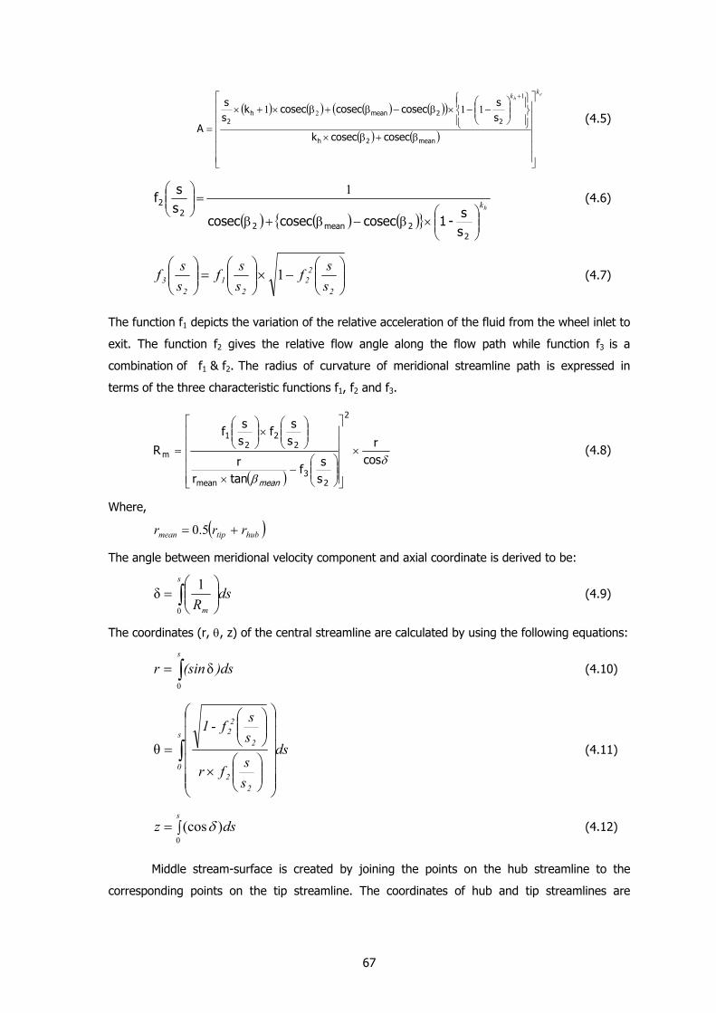
67

( ) ( ) ( ) ( )( )

( ) ( )

eh

kk

⎥⎥⎥⎥⎥⎥

⎦

⎤

⎢⎢⎢⎢⎢⎢

⎣

⎡

β+β×

⎪⎭

⎪⎬⎫

⎪⎩

⎪⎨⎧

⎟⎟⎠

⎞⎜⎜⎝

⎛−−×β−β+β×+×

=

+

mean2h

22meanh

2

coseccoseck

ss

coseccoseccoseckss

A

1

2 111 (4.5)

( ) ( ) ( ){ }hk

⎟⎟⎠

⎞⎜⎜⎝

⎛×β−β+β

=⎟⎟⎠

⎞⎜⎜⎝

⎛

22mean2

22

ss

-1coseccoseccosecss

f1

(4.6)

⎟⎟⎠

⎞⎜⎜⎝

⎛−×⎟⎟

⎠

⎞⎜⎜⎝

⎛=⎟⎟

⎠

⎞⎜⎜⎝

⎛

2

22

21

23 s

sfssf

ssf 1 (4.7)

The function f1 depicts the variation of the relative acceleration of the fluid from the wheel inlet to

exit. The function f2 gives the relative flow angle along the flow path while function f3 is a

combination of f1 & f2. The radius of curvature of meridional streamline path is expressed in

terms of the three characteristic functions f1, f2 and f3.

( )δ

βcos

r

ss

ftanrr

ss

fss

f

R

2

23

mean

22

21

m ×

⎥⎥⎥⎥⎥

⎦

⎤

⎢⎢⎢⎢⎢

⎣

⎡

⎟⎟⎠

⎞⎜⎜⎝

⎛−

×

⎟⎟⎠

⎞⎜⎜⎝

⎛×⎟⎟

⎠

⎞⎜⎜⎝

⎛

=

mean

(4.8)

Where,

( )hubtipmean rrr += 5.0

The angle between meridional velocity component and axial coordinate is derived to be:

∫ ⎟⎟⎠

⎞⎜⎜⎝

⎛=

s

m

dsR0

1δ (4.9)

The coordinates (r, θ, z) of the central streamline are calculated by using the following equations:

∫=s

ds)(sinr0

δ (4.10)

∫⎟⎟⎟⎟⎟⎟

⎠

⎞

⎜⎜⎜⎜⎜⎜

⎝

⎛

⎟⎟⎠

⎞⎜⎜⎝

⎛×

⎟⎟⎠

⎞⎜⎜⎝

⎛

=s

0

22

2

22

ds

ssfr

ssf-1

θ (4.11)

∫=s

dsz0

)(cosδ (4.12)

Middle stream-surface is created by joining the points on the hub streamline to the

corresponding points on the tip streamline. The coordinates of hub and tip streamlines are

68

calculated by using channel depth and the angle between meridional velocity component and

axial coordinate.

To represent the ratio of meridional to circumferential velocity, a characteristics factor is defined

as:

33

3 tanβ==λUCm

m (4.13)

The velocities at different points of meridional streamline are

⎟⎟⎠

⎞⎜⎜⎝

⎛×=

213 ssfCW mm (4.14)

⎟⎟⎠

⎞⎜⎜⎝

⎛=β −

22

1sinssfm (4.15)

mean

m rrU

U×

= 3 (4.16)

β−= cosWUCu (4.17)

⎟⎟⎠

⎞⎜⎜⎝

⎛×⎟⎟⎠

⎞⎜⎜⎝

⎛×=

22

213 s

sfssfCC mm (4.18)

)CC(C um22 += (4.19)

Assuming isentropic flow, the density along the fluid flow path is

11

23

23

23

222

33 2)1(1

−

⎟⎟⎠

⎞⎜⎜⎝

⎛ +−−×

γ−×+×ρ=ρ

m

mCWUWU

mmM (4.20)

The channel width and channel depth at each point are determined by using these equations:

tr

trtrtr Z

tZrw

−βπ=

sin2 (4.21)

mtrtr

tr

CwZm

bρβ

=Δsin

.

(4.22)

The r, θ, z coordinates of the hub and tip streamlines are calculated by using the following

equations:

( )

( )δ

δ

cos2b

rr

cos2b

rr

meantip

meanhub

×Δ

+=

×Δ

−= (4.23)

( )

( )δsin2Δb

zz

δsin2Δb

zz

meantip

meanhub

×−=

×+= (4.24)

69

meanhubtip θθθ == (4.25)

The surface so generated is considered as the mean surface within a blade. The suction

and pressure surfaces of two adjacent channels are computed by translating the mean surface in

the +ve and -ve θ directions through half the blade thickness. The suction side and pressure

side surfaces (r, θ and z coordinates of streamlines) are obtained through the following

equations:

meansuctionpressure rrr == (4.26)

meansuctionpressure zzz == (4.27)

β+θ=θ cos**2 mean

trmeanpressure r

t (4.28)

β−θ=θ cos**2 mean

trmeansuction r

t (4.29)

The average velocity can be split into two parts: one, due to the curvature of the blades

and other, due to the rotation of the blades – the so-called channel-vortex. For turbine wheel,

since the curvature is backward ( bR is positive), the effects are opposite.

The blade angle β along the hub and tip streamlines are calculated by using the following

equations:

⎥⎦

⎤⎢⎣

⎡β×=β − tantan 1

hubhub r

r (4.30)

⎥⎥⎦

⎤

⎢⎢⎣

⎡β×=β − tantan 1

tiptip r

r (4.31)

The velocities of fluid at the suction and pressure sides are determined from the following

expression.

δω2

1 sin.L.R.L.wwb

ss,ps m⎟⎟⎠

⎞⎜⎜⎝

⎛±= (4.32)

where,

β×

⎟⎟⎠

⎞⎜⎜⎝

⎛−

β×⎟⎟⎠

⎞⎜⎜⎝

⎛−=

−cot

1

cos1

2

22

hKh

b

ssC

ecKs

R

1

1211

λ

⎟⎠⎞⎜

⎝⎛ λ−λ+

=C

31 tanβ=λ

70

The thermodynamic quantities are computed using the following relations:

m

PP ⎟⎟⎠

⎞⎜⎜⎝

⎛ρρ

×=3

3 (4.33)

1

33

−

⎟⎟⎠

⎞⎜⎜⎝

⎛ρρ

×=m

TT (4.34)

The results may be used to compute the net axial thrust by integration of the pressure over the

projected area of the turbine wheel.

32

3

2

3

2 prrpdrFr

raxial π+π= ∫↑ (4.35)

( ) 222

2π prrF shaftaxial ×−=↓ (4.36)

Steps of calculations

• Inputs: major dimensions and the flow conditions at the inlet and exit of the wheel

• Determination of the middle streamline

• Determination of the hub and tip streamlines

• Determination of the suction and pressure side geometries of the blade

The block diagram of the computational process using the above algorithm is shown in Figure

4.3. The results of calculation, shown in Figures 4.4 to 4.23, express the interrelationship

between various process and performance parameters.

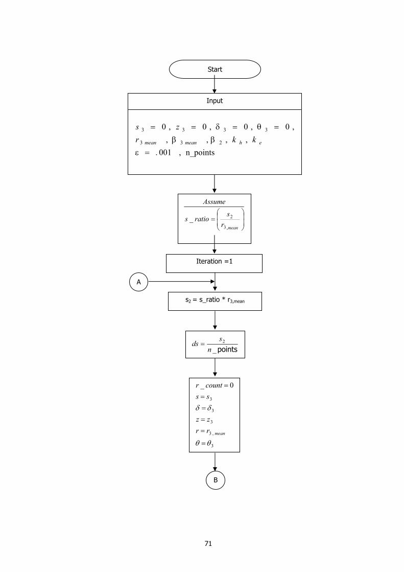
71

Start

⎟⎟⎠

⎞⎜⎜⎝

⎛=

meanrs

ratios

Assume

,3

2_

Iteration =1

s2 = s_ratio * r3,mean

points_2

ns

ds =

3

,3

3

3

3

0_

θθ

δδ

=

====

=

meanrrzz

sscountr

A

Input

n_points,001.,,,,

,0,0,0,0

233

3333

=εββ

=θ=δ==

ehmeanmean kkrzs

B

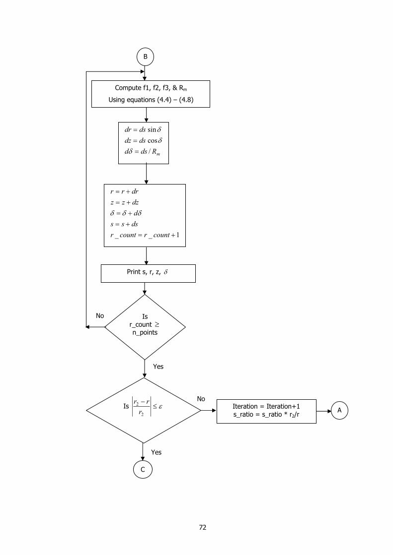
72

Compute f1, f2, f3, & Rm

Using equations (4.4) – (4.8)

mRdsddsdzdsdr

/cossin

===

δδδ

1__ +=+=+=+=+=

countrcountrdsssddzzzdrrr

δδδ

Print s, r, z, δ

Is r_count ≥ n_points

Is ε≤−

2

2

rrr

Iteration = Iteration+1 s_ratio = s_ratio * r2/r

A

C

No

Yes

B

No

Yes

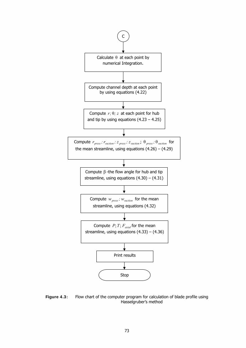
73

Figure 4.3: Flow chart of the computer program for calculation of blade profile using Hasselgruber’s method

Calculate θ at each point by numerical Integration.

Compute channel depth at each point by using equations (4.22)

Compute z;;r θ at each point for hub and tip by using equations (4.23 – 4.25)

C

Compute suctionpresssuctionpress z;z;r;r ; suctionpress ;θθ for

the mean streamline, using equations (4.26) – (4.29)

Print results

Stop

Compute β -the flow angle for hub and tip streamline, using equations (4.30) – (4.31)

Compute suctionpress w;w for the mean

streamline, using equations (4.32)

Compute axialFTP ;; for the mean streamline, using equations (4.33) – (4.36)

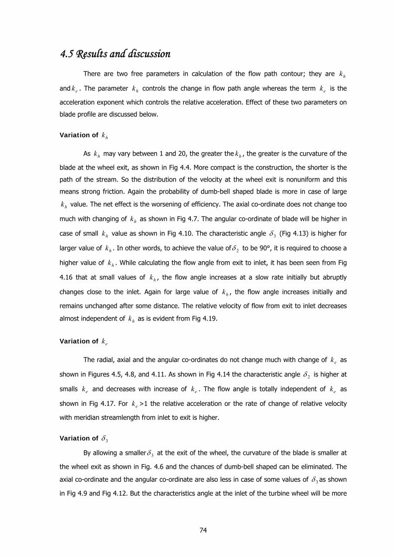
74

4.5 Results and discussion There are two free parameters in calculation of the flow path contour; they are hk

and ek . The parameter hk controls the change in flow path angle whereas the term ek is the

acceleration exponent which controls the relative acceleration. Effect of these two parameters on

blade profile are discussed below.

Variation of hk

As hk may vary between 1 and 20, the greater the hk , the greater is the curvature of the

blade at the wheel exit, as shown in Fig 4.4. More compact is the construction, the shorter is the

path of the stream. So the distribution of the velocity at the wheel exit is nonuniform and this

means strong friction. Again the probability of dumb-bell shaped blade is more in case of large

hk value. The net effect is the worsening of efficiency. The axial co-ordinate does not change too

much with changing of hk as shown in Fig 4.7. The angular co-ordinate of blade will be higher in

case of small hk value as shown in Fig 4.10. The characteristic angle 3δ (Fig 4.13) is higher for

larger value of hk . In other words, to achieve the value of 2δ to be 90°, it is required to choose a

higher value of hk . While calculating the flow angle from exit to inlet, it has been seen from Fig

4.16 that at small values of hk , the flow angle increases at a slow rate initially but abruptly

changes close to the inlet. Again for large value of hk , the flow angle increases initially and

remains unchanged after some distance. The relative velocity of flow from exit to inlet decreases

almost independent of hk as is evident from Fig 4.19.

Variation of ek

The radial, axial and the angular co-ordinates do not change much with change of ek as

shown in Figures 4.5, 4.8, and 4.11. As shown in Fig 4.14 the characteristic angle 2δ is higher at

smalls ek and decreases with increase of ek . The flow angle is totally independent of ek as

shown in Fig 4.17. For ek >1 the relative acceleration or the rate of change of relative velocity

with meridian streamlength from inlet to exit is higher.

Variation of 3δ

By allowing a smaller 3δ at the exit of the wheel, the curvature of the blade is smaller at

the wheel exit as shown in Fig. 4.6 and the chances of dumb-bell shaped can be eliminated. The

axial co-ordinate and the angular co-ordinate are also less in case of some values of 3δ as shown

in Fig 4.9 and Fig 4.12. But the characteristics angle at the inlet of the turbine wheel will be more

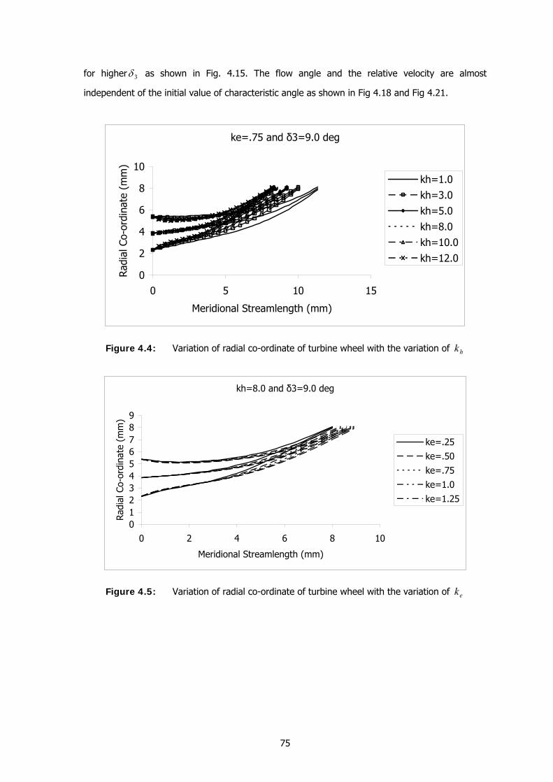
75

for higher 3δ as shown in Fig. 4.15. The flow angle and the relative velocity are almost

independent of the initial value of characteristic angle as shown in Fig 4.18 and Fig 4.21.

ke=.75 and δ3=9.0 deg

0

2

4

6

8

10

0 5 10 15

Meridional Streamlength (mm)

Rad

ial C

o-or

dina

te (

mm

)

kh=1.0kh=3.0kh=5.0kh=8.0kh=10.0kh=12.0

Figure 4.4: Variation of radial co-ordinate of turbine wheel with the variation of hk

kh=8.0 and δ3=9.0 deg

0123456789

0 2 4 6 8 10

Meridional Streamlength (mm)

Rad

ial C

o-or

dina

te (

mm

)

ke=.25ke=.50ke=.75ke=1.0ke=1.25

Figure 4.5: Variation of radial co-ordinate of turbine wheel with the variation of ek

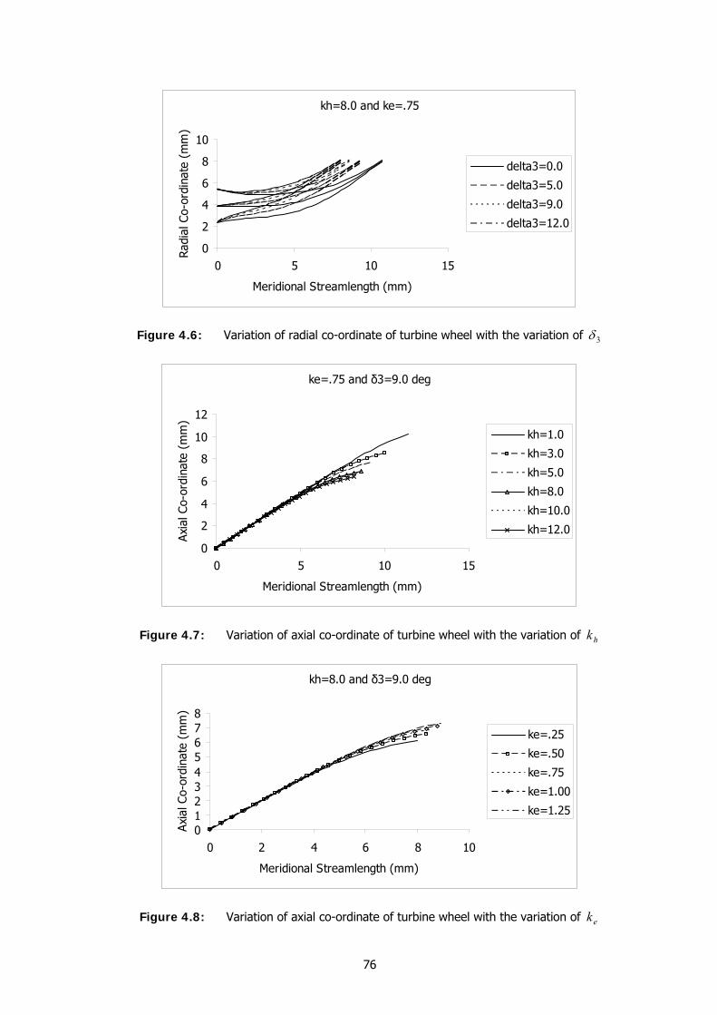
76

kh=8.0 and ke=.75

0

2

4

6

8

10

0 5 10 15

Meridional Streamlength (mm)

Radi

al C

o-or

dina

te (

mm

)delta3=0.0

delta3=5.0

delta3=9.0

delta3=12.0

Figure 4.6: Variation of radial co-ordinate of turbine wheel with the variation of 3δ

ke=.75 and δ3=9.0 deg

0

2

4

6

8

10

12

0 5 10 15

Meridional Streamlength (mm)

Axia

l Co-

ordi

nate

(m

m)

kh=1.0

kh=3.0

kh=5.0

kh=8.0

kh=10.0

kh=12.0

Figure 4.7: Variation of axial co-ordinate of turbine wheel with the variation of hk

kh=8.0 and δ3=9.0 deg

012345678

0 2 4 6 8 10

Meridional Streamlength (mm)

Axia

l Co-

ordi

nate

(m

m)

ke=.25

ke=.50

ke=.75

ke=1.00

ke=1.25

Figure 4.8: Variation of axial co-ordinate of turbine wheel with the variation of ek

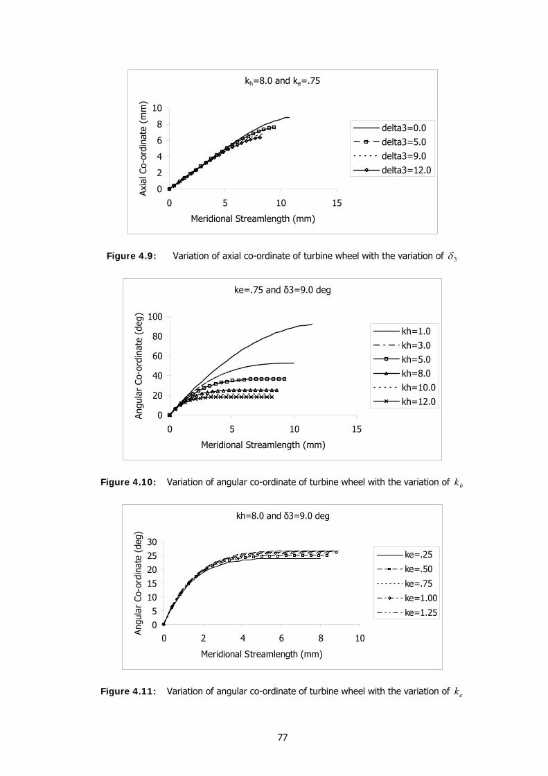
77

kh=8.0 and ke=.75

0

2

4

6

8

10

0 5 10 15

Meridional Streamlength (mm)

Axia

l Co-

ordi

nate

(m

m)

delta3=0.0delta3=5.0delta3=9.0delta3=12.0

Figure 4.9: Variation of axial co-ordinate of turbine wheel with the variation of 3δ

ke=.75 and δ3=9.0 deg

0

20

40

60

80

100

0 5 10 15

Meridional Streamlength (mm)

Angu

lar

Co-o

rdin

ate

(deg

)

kh=1.0kh=3.0kh=5.0kh=8.0kh=10.0kh=12.0

Figure 4.10: Variation of angular co-ordinate of turbine wheel with the variation of hk

kh=8.0 and δ3=9.0 deg

05

1015202530

0 2 4 6 8 10

Meridional Streamlength (mm)

Angu

lar

Co-o

rdin

ate

(deg

)

ke=.25

ke=.50

ke=.75

ke=1.00

ke=1.25

Figure 4.11: Variation of angular co-ordinate of turbine wheel with the variation of ek

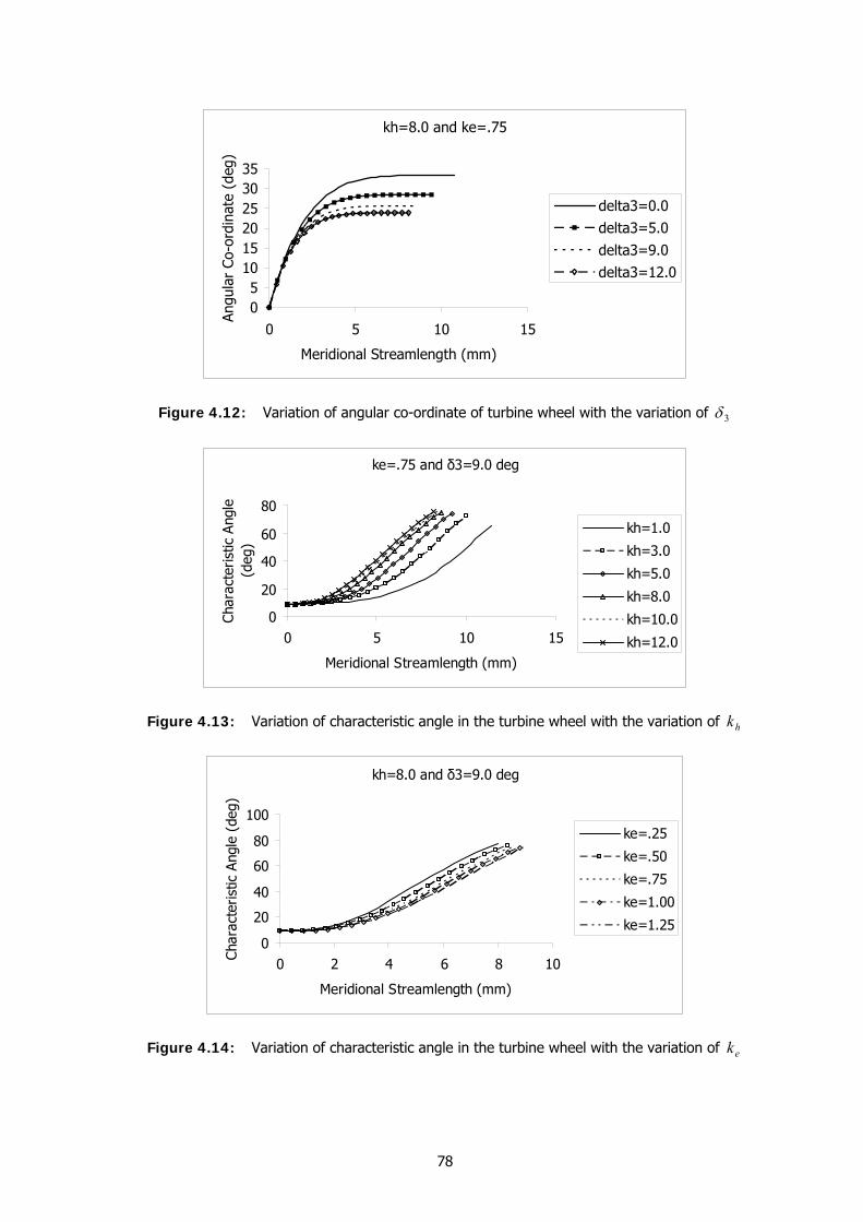
78

kh=8.0 and ke=.75

05

101520253035

0 5 10 15

Meridional Streamlength (mm)

Angu

lar

Co-o

rdin

ate

(deg

)delta3=0.0delta3=5.0delta3=9.0delta3=12.0

Figure 4.12: Variation of angular co-ordinate of turbine wheel with the variation of 3δ

ke=.75 and δ3=9.0 deg

0

20

40

60

80

0 5 10 15

Meridional Streamlength (mm)

Char

acte

ristic

Ang

le

(deg

)

kh=1.0

kh=3.0

kh=5.0

kh=8.0

kh=10.0

kh=12.0

Figure 4.13: Variation of characteristic angle in the turbine wheel with the variation of hk

kh=8.0 and δ3=9.0 deg

0

20

40

60

80

100

0 2 4 6 8 10

Meridional Streamlength (mm)

Char

acte

ristic

Ang

le (

deg)

ke=.25

ke=.50

ke=.75

ke=1.00

ke=1.25

Figure 4.14: Variation of characteristic angle in the turbine wheel with the variation of ek

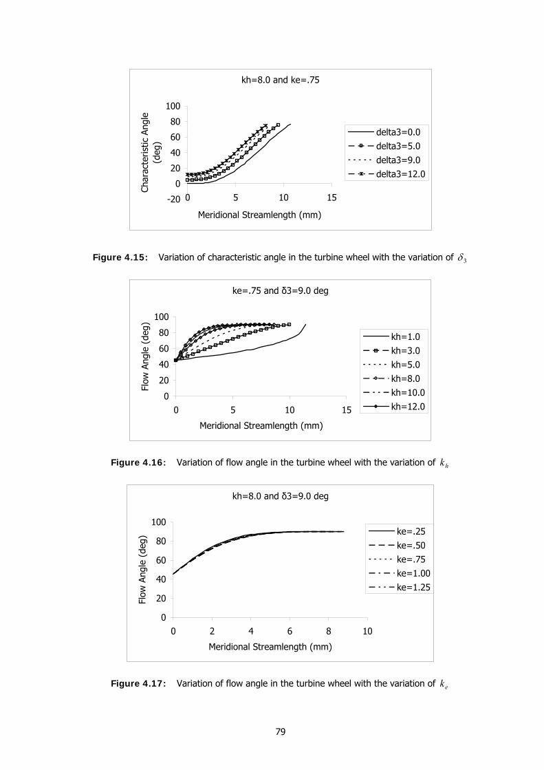
79

kh=8.0 and ke=.75

-20

0

20

40

60

80

100

0 5 10 15

Meridional Streamlength (mm)

Char

acte

ristic

Ang

le

(deg

)

delta3=0.0delta3=5.0delta3=9.0delta3=12.0

Figure 4.15: Variation of characteristic angle in the turbine wheel with the variation of 3δ

ke=.75 and δ3=9.0 deg

0

20

40

60

80

100

0 5 10 15

Meridional Streamlength (mm)

Flow

Ang

le (

deg)

kh=1.0kh=3.0kh=5.0kh=8.0kh=10.0kh=12.0

Figure 4.16: Variation of flow angle in the turbine wheel with the variation of hk

kh=8.0 and δ3=9.0 deg

0

20

40

60

80

100

0 2 4 6 8 10

Meridional Streamlength (mm)

Flow

Ang

le (

deg)

ke=.25ke=.50ke=.75ke=1.00ke=1.25

Figure 4.17: Variation of flow angle in the turbine wheel with the variation of ek

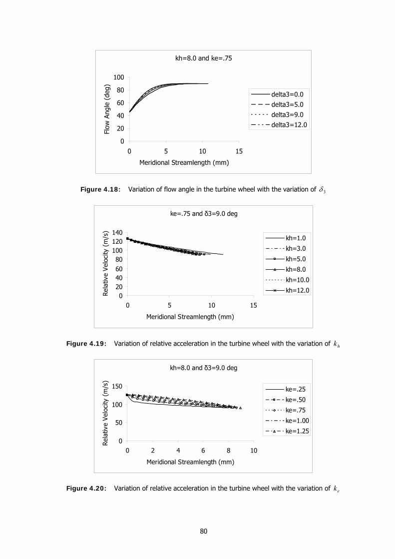
80

kh=8.0 and ke=.75

0

20

40

60

80

100

0 5 10 15

Meridional Streamlength (mm)

Flow

Ang

le (

deg)

delta3=0.0delta3=5.0delta3=9.0delta3=12.0

Figure 4.18: Variation of flow angle in the turbine wheel with the variation of 3δ

ke=.75 and δ3=9.0 deg

020406080

100120140

0 5 10 15

Meridional Streamlength (mm)

Rela

tive

Velo

city

(m

/s)

kh=1.0

kh=3.0

kh=5.0

kh=8.0

kh=10.0

kh=12.0

Figure 4.19: Variation of relative acceleration in the turbine wheel with the variation of hk

kh=8.0 and δ3=9.0 deg

0

50

100

150

0 2 4 6 8 10

Meridional Streamlength (mm)

Rela

tive

Velo

city

(m

/s)

ke=.25

ke=.50

ke=.75

ke=1.00

ke=1.25

Figure 4.20: Variation of relative acceleration in the turbine wheel with the variation of ek

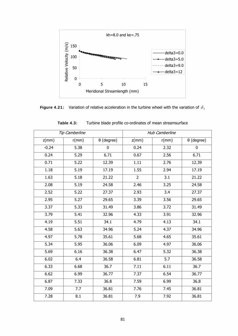
81

kh=8.0 and ke=.75

0

50

100

150

0 5 10 15

Meridional Streamlength (mm)

Rela

tive

Velo

city

(m

/s)

delta3=0.0

delta3=5.0

delta3=9.0

delta3=12

Figure 4.21: Variation of relative acceleration in the turbine wheel with the variation of 3δ

Table 4.3: Turbine blade profile co-ordinates of mean streamsurface Tip Camberline Hub Camberline

z(mm) r(mm) θ (degree) z(mm) r(mm) θ (degree)

-0.24 5.38 0 0.24 2.32 0

0.24 5.29 6.71 0.67 2.56 6.71

0.71 5.22 12.39 1.11 2.76 12.39

1.18 5.19 17.19 1.55 2.94 17.19

1.63 5.18 21.22 2 3.1 21.22

2.08 5.19 24.58 2.46 3.25 24.58

2.52 5.22 27.37 2.93 3.4 27.37

2.95 5.27 29.65 3.39 3.56 29.65

3.37 5.33 31.49 3.86 3.72 31.49

3.79 5.41 32.96 4.33 3.91 32.96

4.19 5.51 34.1 4.79 4.13 34.1

4.58 5.63 34.96 5.24 4.37 34.96

4.97 5.78 35.61 5.68 4.65 35.61

5.34 5.95 36.06 6.09 4.97 36.06

5.69 6.16 36.38 6.47 5.32 36.38

6.02 6.4 36.58 6.81 5.7 36.58

6.33 6.68 36.7 7.11 6.11 36.7

6.62 6.99 36.77 7.37 6.54 36.77

6.87 7.33 36.8 7.59 6.99 36.8

7.09 7.7 36.81 7.76 7.45 36.81

7.28 8.1 36.81 7.9 7.92 36.81

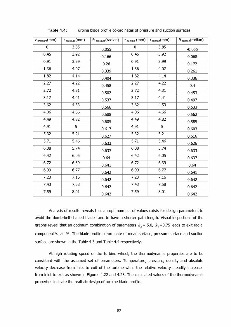
82

Table 4.4: Turbine blade profile co-ordinates of pressure and suction surfaces z pressure(mm) r pressure(mm) θ pressure(radian) z suction (mm) r suction(mm) θ suction(radian)

0 3.85 0.055 0 3.85 -0.055 0.45 3.92 0.166 0.45 3.92 0.068 0.91 3.99 0.26 0.91 3.99 0.172 1.36 4.07 0.339 1.36 4.07 0.261 1.82 4.14 0.404 1.82 4.14 0.336 2.27 4.22 0.458 2.27 4.22 0.4 2.72 4.31 0.502 2.72 4.31 0.453 3.17 4.41 0.537 3.17 4.41 0.497 3.62 4.53 0.566 3.62 4.53 0.533 4.06 4.66 0.588 4.06 4.66 0.562 4.49 4.82 0.605 4.49 4.82 0.585 4.91 5 0.617 4.91 5 0.603 5.32 5.21 0.627 5.32 5.21 0.616 5.71 5.46 0.633 5.71 5.46 0.626 6.08 5.74 0.637 6.08 5.74 0.633 6.42 6.05 0.64 6.42 6.05 0.637 6.72 6.39 0.641 6.72 6.39 0.64 6.99 6.77 0.642 6.99 6.77 0.641 7.23 7.16 0.642 7.23 7.16 0.642 7.43 7.58 0.642 7.43 7.58 0.642 7.59 8.01 0.642 7.59 8.01 0.642

Analysis of results reveals that an optimum set of values exists for design parameters to

avoid the dumb-bell shaped blades and to have a shorter path length. Visual inspections of the

graphs reveal that an optimum combination of parameters hk = 5.0, ek =0.75 leads to exit radial

component 3δ as 9°. The blade profile co-ordinate of mean surface, pressure surface and suction

surface are shown in the Table 4.3 and Table 4.4 respectively.

At high rotating speed of the turbine wheel, the thermodynamic properties are to be

consistant with the assumed set of parameters. Temperature, pressure, density and absolute

velocity decrease from inlet to exit of the turbine while the relative velocity steadily increases

from inlet to exit as shown in Figures 4.22 and 4.23. The calculated values of the thermodynamic

properties indicate the realistic design of turbine blade profile.

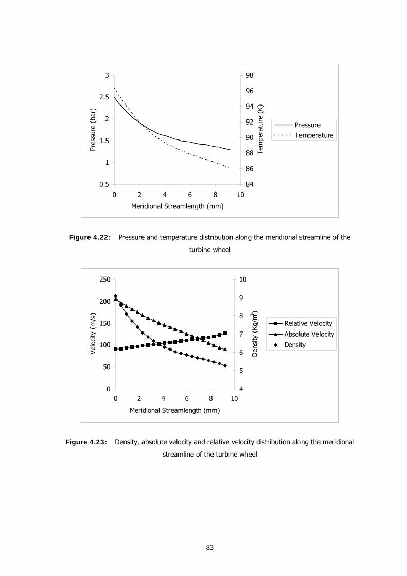
83

0.5

1

1.5

2

2.5

3

0 2 4 6 8 10

Meridional Streamlength (mm)

Pres

sure

(ba

r)

84

86

88

90

92

94

96

98

Tem

pera

ture

(K)

PressureTemperature

Figure 4.22: Pressure and temperature distribution along the meridional streamline of the

turbine wheel

0

50

100

150

200

250

0 2 4 6 8 10

Meridional Streamlength (mm)

Velo

city

(m

/s)

4

5

6

7

8

9

10

Den

sity

(Kg

/m3 )

Relative Velocity

Absolute Velocity

Density

Figure 4.23: Density, absolute velocity and relative velocity distribution along the meridional

streamline of the turbine wheel

Chapter 5

Development of Prototype

Turboexpander

Chapter V

DEVELOPMENT OF PROTOTYPE

TURBOEXPANDER

The work presented in this chapter is aimed at the development of a small high speed

cryogenic turboexpander. A cryogenic turboexpander is a precision equipment. For high speed

and the clearances of 10 to 40 μm in the bearings the rotor should be properly balanced. This

demands micron scale manufacturing tolerance in the shaft and the impeller. The need for

precision excludes the use of casting and forging in fabrication of major components. Metal

cutting, using precision and CNC machine tools, is the most practical means of fabricating a

cryogenic turbine. A review has been done on material selection, tolerance analysis, fabrication

and assembly of the turboexpander.

5.1 Materials for the Turbine System Selection of materials is an important aspect of the design process. Austenitic stainless

steel (SS 304), widely used in cryogenic engineering applications owing to its low thermal

conductivity, high strength, stiffness, toughness and corrosion resistance, is chosen as the

common material for all structural components. Special materials, however, have to be selected

for critical components such as turbine wheel, brake compressor impeller, shaft, bearings, seals

and fasteners. The materials selection process takes into consideration of the following factors:

• yield strength,

• ductility and fatigue strength,

• density,

• thermal conductivity,

• coefficient of thermal expansion,

• machinability and ease of fabrication.

For a rotating solid disc of uniform thickness, the collapse speed is given by the equation [116]:

col

Y

colcollapse R

Nρσ

π3

260

= (5.1)

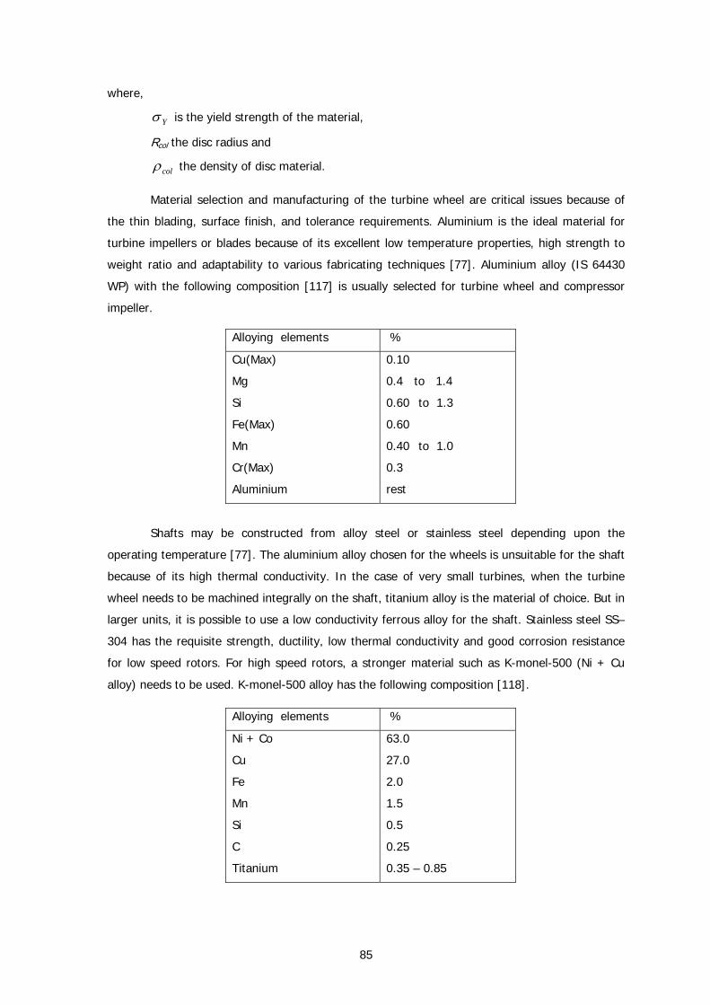
85

where,

Yσ is the yield strength of the material,

Rcol the disc radius and

colρ the density of disc material.

Material selection and manufacturing of the turbine wheel are critical issues because of

the thin blading, surface finish, and tolerance requirements. Aluminium is the ideal material for

turbine impellers or blades because of its excellent low temperature properties, high strength to

weight ratio and adaptability to various fabricating techniques [77]. Aluminium alloy (IS 64430

WP) with the following composition [117] is usually selected for turbine wheel and compressor

impeller.

Alloying elements %

Cu(Max)

Mg

Si

Fe(Max)

Mn

Cr(Max)

Aluminium

0.10

0.4 to 1.4

0.60 to 1.3

0.60

0.40 to 1.0

0.3

rest

Shafts may be constructed from alloy steel or stainless steel depending upon the

operating temperature [77]. The aluminium alloy chosen for the wheels is unsuitable for the shaft

because of its high thermal conductivity. In the case of very small turbines, when the turbine

wheel needs to be machined integrally on the shaft, titanium alloy is the material of choice. But in

larger units, it is possible to use a low conductivity ferrous alloy for the shaft. Stainless steel SS–

304 has the requisite strength, ductility, low thermal conductivity and good corrosion resistance

for low speed rotors. For high speed rotors, a stronger material such as K-monel-500 (Ni + Cu

alloy) needs to be used. K-monel-500 alloy has the following composition [118].

Alloying elements %

Ni + Co

Cu

Fe

Mn

Si

C

Titanium

63.0

27.0

2.0

1.5

0.5

0.25

0.35 – 0.85

86

To keep parity with the rest of the components, and to eliminate change of clearances

and stresses due to differential thermal expansion the material should be carefully chosen. The

thrust plates are made from phosphor bronze, which has been chosen for its good machinability

and compatibility with stainless steel. To avoid differential contraction, tilting pad journal bearing

pad housing is made of Monel K-500 and the bearing pads are made from high-density metal

impregnated graphite. The material is moderately soft and self-lubricating. It can tolerate rubbing

during start-ups and shutdowns. It is, however, difficult to maintain dimensional accuracy during

machining, and utmost care is required in this work. The end pad plate is made from SS 304.

Effective shaft sealing is extremely important in turboexpanders since the power

expended on the refrigerant generally makes it quite valuable [77]. Simple labyrinths can be used

with relatively good results where the differential pressure across the seal is quite low. Other

materials used in the system include neoprene rubber for the static seals.

5.2 Analysis of Design Tolerance

Tolerance analysis is a valuable tool for improving product quality and reducing

manufacturing cost. Tolerances also greatly influence the selection of production process and

determine the assemblability of the final product. The assignment of tolerances to individual

component dimension is important to ensure that the product is produced economically and

functions properly. The designers may assign relatively tight tolerances to ensure that the

product performs correctly, albeit at a higher manufacturing cost. Relaxing tolerances on each

component, on the other hand, reduces costs, but can result in unacceptable loss of quality and

high scrap rate, leading to customer dissatisfaction. These conflicting goals point out the need for

methods to rationally assign tolerances to products so that customers can be provided with high

quality products at competitive market prices.

The turbine wheel Tolerancing of the wheel must satisfy the following requirements:

i). The clearance between the wheel and diffuser shroud should remain within the

prescribed limits, and

ii). Its surface roughness should be maintained better than the prescribed value.

It may be noted that the aluminium alloy, used for fabrication of the wheel, has a tendency to

flow during machining [119] making it difficult to achieve high precision.

For presenting geometrical tolerances on the dimensions of the wheel, the back face of

the wheel has been chosen as the datum. The flatness of this face has been specified to be

within 5 μm. The tolerances that affect the clearance between the wheel tip and the shroud are:

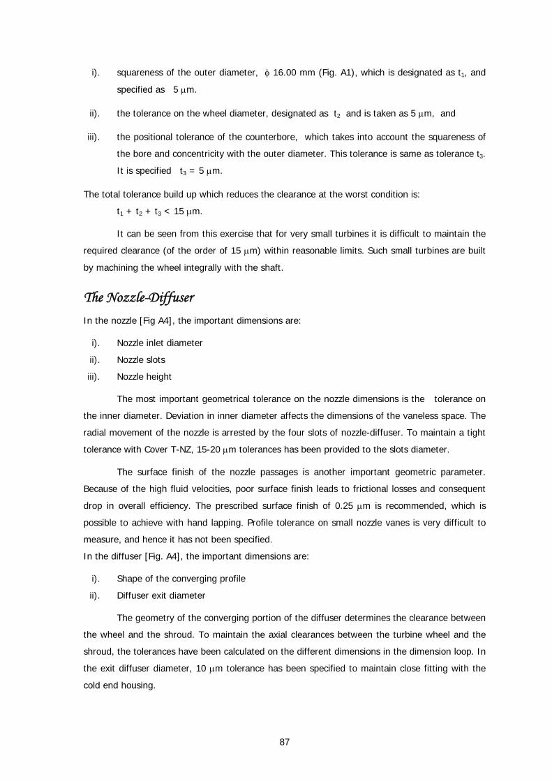
87

i). squareness of the outer diameter, φ 16.00 mm (Fig. A1), which is designated as t1, and

specified as 5 μm.

ii). the tolerance on the wheel diameter, designated as t2 and is taken as 5 μm, and

iii). the positional tolerance of the counterbore, which takes into account the squareness of

the bore and concentricity with the outer diameter. This tolerance is same as tolerance t3.

It is specified t3 = 5 μm.

The total tolerance build up which reduces the clearance at the worst condition is:

t1 + t2 + t3 < 15 μm.

It can be seen from this exercise that for very small turbines it is difficult to maintain the

required clearance (of the order of 15 μm) within reasonable limits. Such small turbines are built

by machining the wheel integrally with the shaft.

The Nozzle-Diffuser In the nozzle [Fig A4], the important dimensions are:

i). Nozzle inlet diameter

ii). Nozzle slots

iii). Nozzle height

The most important geometrical tolerance on the nozzle dimensions is the tolerance on

the inner diameter. Deviation in inner diameter affects the dimensions of the vaneless space. The

radial movement of the nozzle is arrested by the four slots of nozzle-diffuser. To maintain a tight

tolerance with Cover T-NZ, 15-20 μm tolerances has been provided to the slots diameter.

The surface finish of the nozzle passages is another important geometric parameter.

Because of the high fluid velocities, poor surface finish leads to frictional losses and consequent

drop in overall efficiency. The prescribed surface finish of 0.25 μm is recommended, which is

possible to achieve with hand lapping. Profile tolerance on small nozzle vanes is very difficult to

measure, and hence it has not been specified.

In the diffuser [Fig. A4], the important dimensions are:

i). Shape of the converging profile

ii). Diffuser exit diameter

The geometry of the converging portion of the diffuser determines the clearance between

the wheel and the shroud. To maintain the axial clearances between the turbine wheel and the

shroud, the tolerances have been calculated on the different dimensions in the dimension loop. In

the exit diffuser diameter, 10 μm tolerance has been specified to maintain close fitting with the

cold end housing.

88

The shaft and the bearings

The shaft and the bearings constitute the most critical components of the system. High

dimensional accuracy of these components is necessary not only to maintain required clearances,

but also to avoid balancing problems and rotodynamic instabilities. The shaft should have a

cylindricity and surface roughness below 2μm and 0.2μm respectively. Good cylindricity is an

absolute necessity, because both bearing clearance and rotor stability are adversely affected by

ovality of the shaft [120]. The bearing bore and the shaft diameter, which determine the bearing

clearance, have been designed in H4f4 class. The hole is chosen as the basis of tolerance,

because it is much easier to grind the outer cylindrical surface of a shaft to required size than to

finish the bore of a bearing. To prevent large difference from the designed clearance, the thrust

collar is given a dimensional tolerance of 5μm. This, along with a similar tolerance on thrust plate

spacer, limits the maximum variation of thrust clearance to within 10μm. The thrust bearing faces

must be perpendicular to the datum reference (the journal axis) to within 2μm. A radial clearance

of 10-15 μm with the journal bearing is provided with a tolerance of 5 μm.

The bearing housing

The bearing housing is the central component of the structural system, accommodating

all the precision components. In general, manufacturing tolerance is kept as loose as possible for

a large component like the bearing housing. However, for some of the features, a tight tolerance

is absolutely necessary. The extreme faces of the housing are taken as datum surfaces and

should be straight with a flatness specification of 2 μm, which is not very difficult to achieve

[121]. The datum axis is defined by the inner diameter. Features like thrust plate seat must be

maintained within the set tolerances on flatness and perpendicularity. It has been prescribed

perpendicularity of 3 to 5 μm, which can be achieved by surface grinding [121].

Length tolerance analysis

The dependence of critical clearances in an assembly on manufacturing tolerance of the

components must be analysed to ensure that the clearances remain within acceptable limits.

Although it has not been possible to implement the best practices in tolerancing because of

unavailability of proper facilities, the method described by Fortini [122] has been followed to

carry out such analysis on four critical clearances in the turbine system. They can be described

as:

i). the clearance in the thrust bearings,

ii). clearance between the turbine wheel and the shroud,

iii). clearance between journal bearing and shaft, and

iv). clearance between brake compressor and the lock nut behind it.

89

A dimension loop may consist of a closed set of vectors; one vector represents the

dimension condition and the other vectors represent the dimensions, controlling the dimension

condition. The dimension of one of these components, usually a clearance or an interference, is

called the “dimension condition”. The direction of the vector of dimension condition is always

taken to be positive. The dimension condition is symbolized by wy which is a function of the

independent dimensions ix ( ni −=1 ), the direction of ix being either positive or negative

depending on the nature of their alignment with wy .

Some vectors in a dimension loop have restricted values; their values are predetermined

because the parts may be standard or the dimensions of the parts may be involved in other

dimension loops. In making detailed calculations, the general approach is to assign numerical

values for the magnitudes of all except one dimension vector. The value of the unknown

dimension vector is then obtained by a simple calculation. The general equation for a dimension

loop is

( ) ( ) ( ) 0=−∑−+∑++ xxyw

This equation makes the statement that the sum of all the vectors in a closed loop is

zero. The convention is followed that the positive direction is always the direction of the

dimension condition.

On the basis of worst limit calculation the limit values of dimensions is determined by the

following set of equations

∑=

=−=−n

iitLLULwW

1

∑∑+

=

−

=

+−−=n

ii

n

ii xxW

1min,

1max, )()(

∑∑+

=

−

=

+−−=n

ii

n

ii xxw

1max,

1min, )()(

where,

W = the maximum value of ULyy ww +=

w = the minimum value of LLyy ww +=

it is the tolerance of the thi dimension, ix and n being the total number of such independent

dimensions. ‘ x+ ’ and ‘ x− ’ are the positive and negative dimensions, and ‘ +n ’ and ‘ −n ‘

refer to the total number of such dimensions. The subscripts ‘ imax ’ and ‘ imin ’ refer to the

highest and the lowest values of the thi dimension.

Some tolerances in a loop may be restricted by process requirements, the others being

relaxed. The sum of the tolerances for unrestricted dimensions can be assigned in many ways.

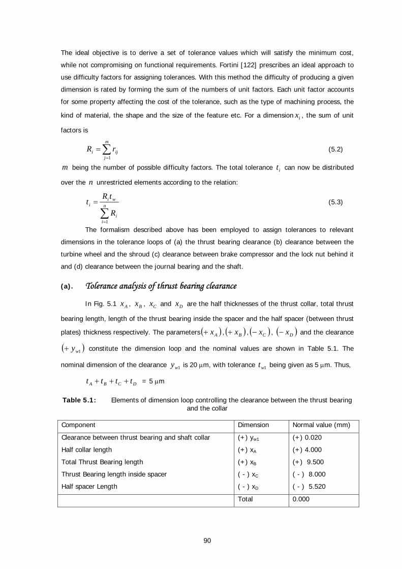
90

The ideal objective is to derive a set of tolerance values which will satisfy the minimum cost,

while not compromising on functional requirements. Fortini [122] prescribes an ideal approach to

use difficulty factors for assigning tolerances. With this method the difficulty of producing a given

dimension is rated by forming the sum of the numbers of unit factors. Each unit factor accounts

for some property affecting the cost of the tolerance, such as the type of machining process, the

kind of material, the shape and the size of the feature etc. For a dimension ix , the sum of unit

factors is

∑=

=m

jiji rR

1 (5.2)

m being the number of possible difficulty factors. The total tolerance it can now be distributed

over the n unrestricted elements according to the relation:

∑=

= n

ii

wii

R

tRt

1

(5.3)

The formalism described above has been employed to assign tolerances to relevant

dimensions in the tolerance loops of (a) the thrust bearing clearance (b) clearance between the

turbine wheel and the shroud (c) clearance between brake compressor and the lock nut behind it

and (d) clearance between the journal bearing and the shaft.

(a). Tolerance analysis of thrust bearing clearance

In Fig. 5.1 Ax , Bx , Cx and Dx are the half thicknesses of the thrust collar, total thrust

bearing length, length of the thrust bearing inside the spacer and the half spacer (between thrust

plates) thickness respectively. The parameters ( )Ax+ , ( )Bx+ , ( )Cx− , ( )Dx− and the clearance

( )1wy+ constitute the dimension loop and the nominal values are shown in Table 5.1. The

nominal dimension of the clearance 1wy is 20 μm, with tolerance 1wt being given as 5 μm. Thus,

DCBA tttt +++ = 5 μm

Table 5.1: Elements of dimension loop controlling the clearance between the thrust bearing

and the collar

Component Dimension Normal value (mm)

Clearance between thrust bearing and shaft collar

Half collar length

Total Thrust Bearing length

Thrust Bearing length inside spacer

Half spacer Length

(+) yw1

(+) xA

(+) xB

( - ) xC

( - ) xD

(+) 0.020

(+) 4.000

(+) 9.500

( - ) 8.000

( - ) 5.520

Total 0.000

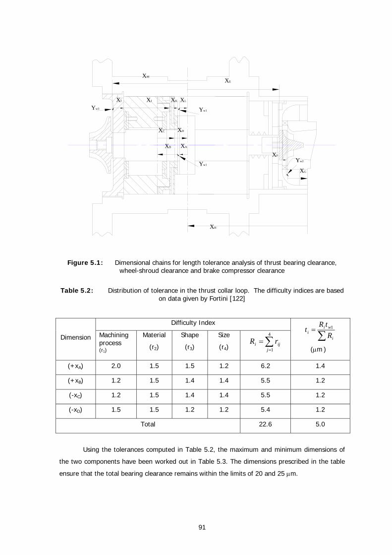
91

XAXB

XC XD

XE

XF

XG

XH

XI XJ XK XL

XM

Yw1Yw2

Yw3 Yw1

Figure 5.1: Dimensional chains for length tolerance analysis of thrust bearing clearance, wheel-shroud clearance and brake compressor clearance

Table 5.2: Distribution of tolerance in the thrust collar loop. The difficulty indices are based on data given by Fortini [122]

Difficulty Index

Dimension Machining process (r1)

Material

(r2)

Shape

(r3)

Size

(r4) ∑=

=4

1jiji rR

∑=

i

wii R

tRt 1

(μm )

(+xA) 2.0 1.5 1.5 1.2 6.2 1.4

(+xB) 1.2 1.5 1.4 1.4 5.5 1.2

(-xC) 1.2 1.5 1.4 1.4 5.5 1.2

(-xD) 1.5 1.5 1.2 1.2 5.4 1.2

Total 22.6 5.0

Using the tolerances computed in Table 5.2, the maximum and minimum dimensions of

the two components have been worked out in Table 5.3. The dimensions prescribed in the table

ensure that the total bearing clearance remains within the limits of 20 and 25 μm.

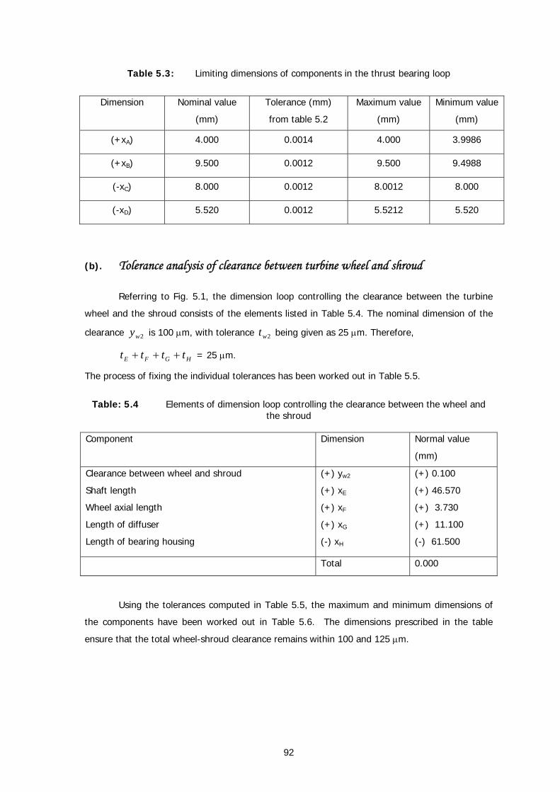
92

Table 5.3: Limiting dimensions of components in the thrust bearing loop

Dimension Nominal value

(mm)

Tolerance (mm)

from table 5.2

Maximum value

(mm)

Minimum value

(mm)

(+xA) 4.000 0.0014 4.000 3.9986

(+xB) 9.500 0.0012 9.500 9.4988

(-xC) 8.000 0.0012 8.0012 8.000

(-xD) 5.520 0.0012 5.5212 5.520

(b). Tolerance analysis of clearance between turbine wheel and shroud

Referring to Fig. 5.1, the dimension loop controlling the clearance between the turbine

wheel and the shroud consists of the elements listed in Table 5.4. The nominal dimension of the

clearance 2wy is 100 μm, with tolerance 2wt being given as 25 μm. Therefore,

HGFE tttt +++ = 25 μm.

The process of fixing the individual tolerances has been worked out in Table 5.5.

Table: 5.4 Elements of dimension loop controlling the clearance between the wheel and the shroud

Component Dimension Normal value

(mm)

Clearance between wheel and shroud

Shaft length

Wheel axial length

Length of diffuser

Length of bearing housing

(+) yw2

(+) xE

(+) xF

(+) xG

(-) xH

(+) 0.100

(+) 46.570

(+) 3.730

(+) 11.100

(-) 61.500

Total 0.000

Using the tolerances computed in Table 5.5, the maximum and minimum dimensions of

the components have been worked out in Table 5.6. The dimensions prescribed in the table

ensure that the total wheel-shroud clearance remains within 100 and 125 μm.

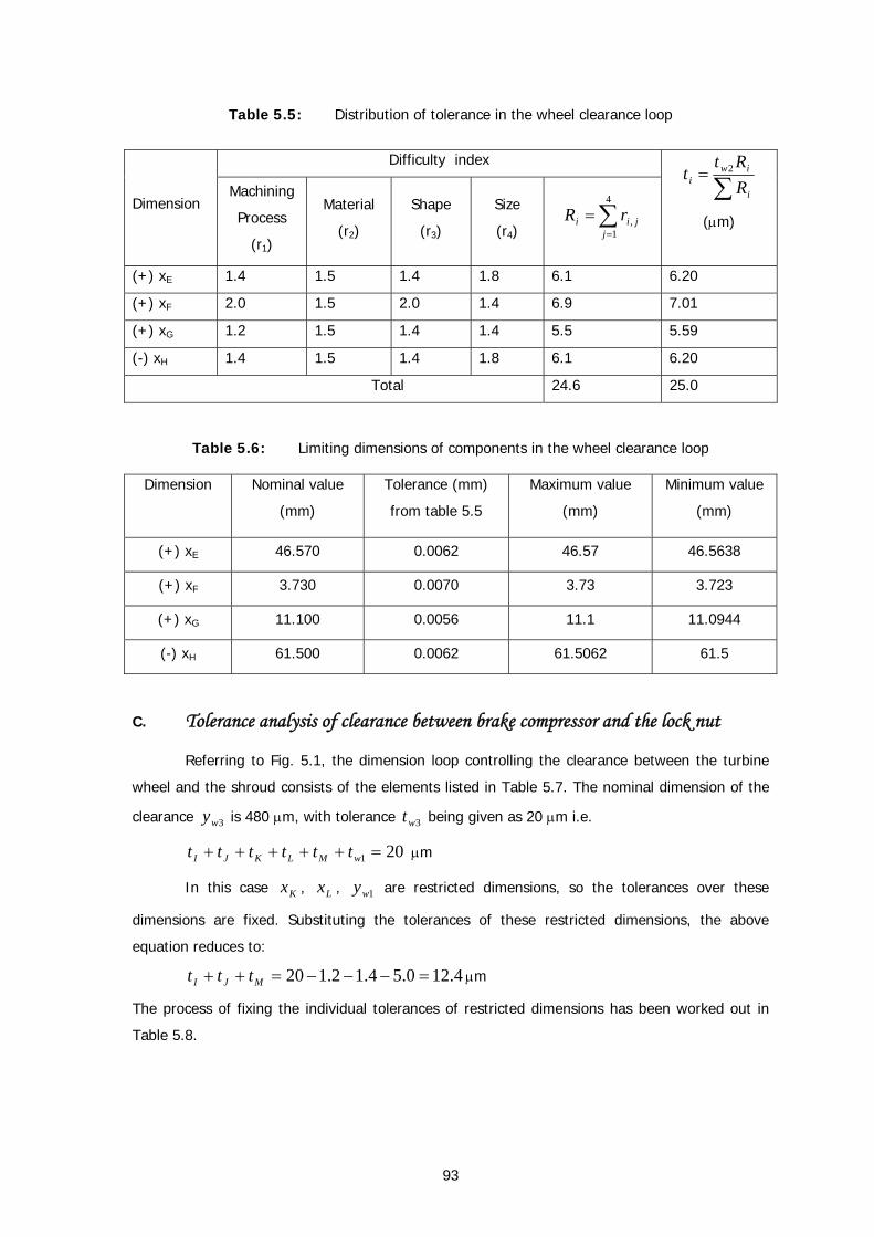
93

Table 5.5: Distribution of tolerance in the wheel clearance loop

Difficulty index

Dimension Machining

Process

(r1)

Material

(r2)

Shape

(r3)

Size

(r4) ∑=

=4

1,

jjii rR

∑=

i

iwi R

Rtt 2

(μm)

(+) xE 1.4 1.5 1.4 1.8 6.1 6.20

(+) xF 2.0 1.5 2.0 1.4 6.9 7.01

(+) xG 1.2 1.5 1.4 1.4 5.5 5.59

(-) xH 1.4 1.5 1.4 1.8 6.1 6.20

Total 24.6 25.0

Table 5.6: Limiting dimensions of components in the wheel clearance loop

Dimension Nominal value

(mm)

Tolerance (mm)

from table 5.5

Maximum value

(mm)

Minimum value

(mm)

(+) xE 46.570 0.0062 46.57 46.5638

(+) xF 3.730 0.0070 3.73 3.723

(+) xG 11.100 0.0056 11.1 11.0944

(-) xH 61.500 0.0062 61.5062 61.5

C. Tolerance analysis of clearance between brake compressor and the lock nut

Referring to Fig. 5.1, the dimension loop controlling the clearance between the turbine

wheel and the shroud consists of the elements listed in Table 5.7. The nominal dimension of the

clearance 3wy is 480 μm, with tolerance 3wt being given as 20 μm i.e.

201 =+++++ wMLKJI tttttt μm

In this case Kx , Lx , 1wy are restricted dimensions, so the tolerances over these

dimensions are fixed. Substituting the tolerances of these restricted dimensions, the above

equation reduces to:

4.120.54.12.120 =−−−=++ MJI ttt μm

The process of fixing the individual tolerances of restricted dimensions has been worked out in

Table 5.8.

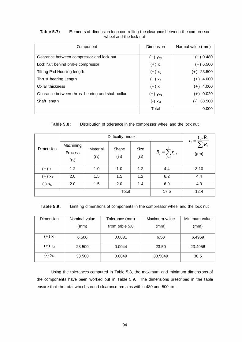
94

Table 5.7: Elements of dimension loop controlling the clearance between the compressor wheel and the lock nut

Component Dimension Normal value (mm)

Clearance between compressor and lock nut

Lock Nut behind brake compressor

Tilting Pad Housing length

Thrust bearing Length

Collar thickness

Clearance between thrust bearing and shaft collar

Shaft length

(+) yw3

(+) xI

(+) xJ

(+) xK

(+) xL

(+) yw1

(-) xM

(+) 0.480

(+) 6.500

(+) 23.500

(+) 4.000

(+) 4.000

(+) 0.020

(-) 38.500

Total 0.000

Table 5.8: Distribution of tolerance in the compressor wheel and the lock nut

Difficulty index

Dimension Machining

Process

(r1)

Material

(r2)

Shape

(r3)

Size

(r4) ∑=

=4

1,

jjii rR

∑=

i

iwi R

Rtt 2

(μm)

(+) xI 1.2 1.0 1.0 1.2 4.4 3.10

(+) xJ 2.0 1.5 1.5 1.2 6.2 4.4

(-) xM 2.0 1.5 2.0 1.4 6.9 4.9

Total 17.5 12.4

Table 5.9: Limiting dimensions of components in the compressor wheel and the lock nut

Dimension Nominal value

(mm)

Tolerance (mm)

from table 5.8

Maximum value

(mm)

Minimum value

(mm)

(+) xI 6.500 0.0031 6.50 6.4969

(+) xJ 23.500 0.0044 23.50 23.4956

(-) xM 38.500 0.0049 38.5049 38.5

Using the tolerances computed in Table 5.8, the maximum and minimum dimensions of

the components have been worked out in Table 5.9. The dimensions prescribed in the table

ensure that the total wheel-shroud clearance remains within 480 and 500 μm.

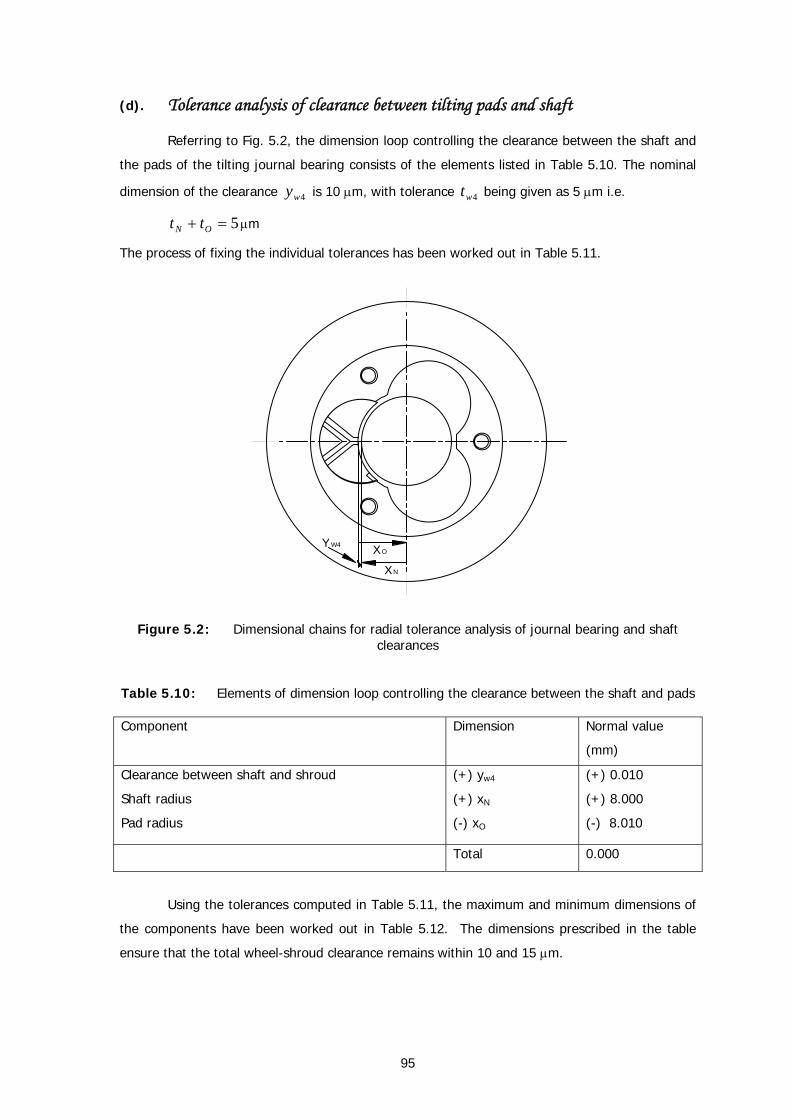
95

(d). Tolerance analysis of clearance between tilting pads and shaft

Referring to Fig. 5.2, the dimension loop controlling the clearance between the shaft and

the pads of the tilting journal bearing consists of the elements listed in Table 5.10. The nominal

dimension of the clearance 4wy is 10 μm, with tolerance 4wt being given as 5 μm i.e.

5=+ ON tt μm

The process of fixing the individual tolerances has been worked out in Table 5.11.

Figure 5.2: Dimensional chains for radial tolerance analysis of journal bearing and shaft clearances

Table 5.10: Elements of dimension loop controlling the clearance between the shaft and pads

Component Dimension Normal value

(mm)

Clearance between shaft and shroud

Shaft radius

Pad radius

(+) yw4

(+) xN

(-) xO

(+) 0.010

(+) 8.000

(-) 8.010

Total 0.000

Using the tolerances computed in Table 5.11, the maximum and minimum dimensions of

the components have been worked out in Table 5.12. The dimensions prescribed in the table

ensure that the total wheel-shroud clearance remains within 10 and 15 μm.

Y W4 X O

X N

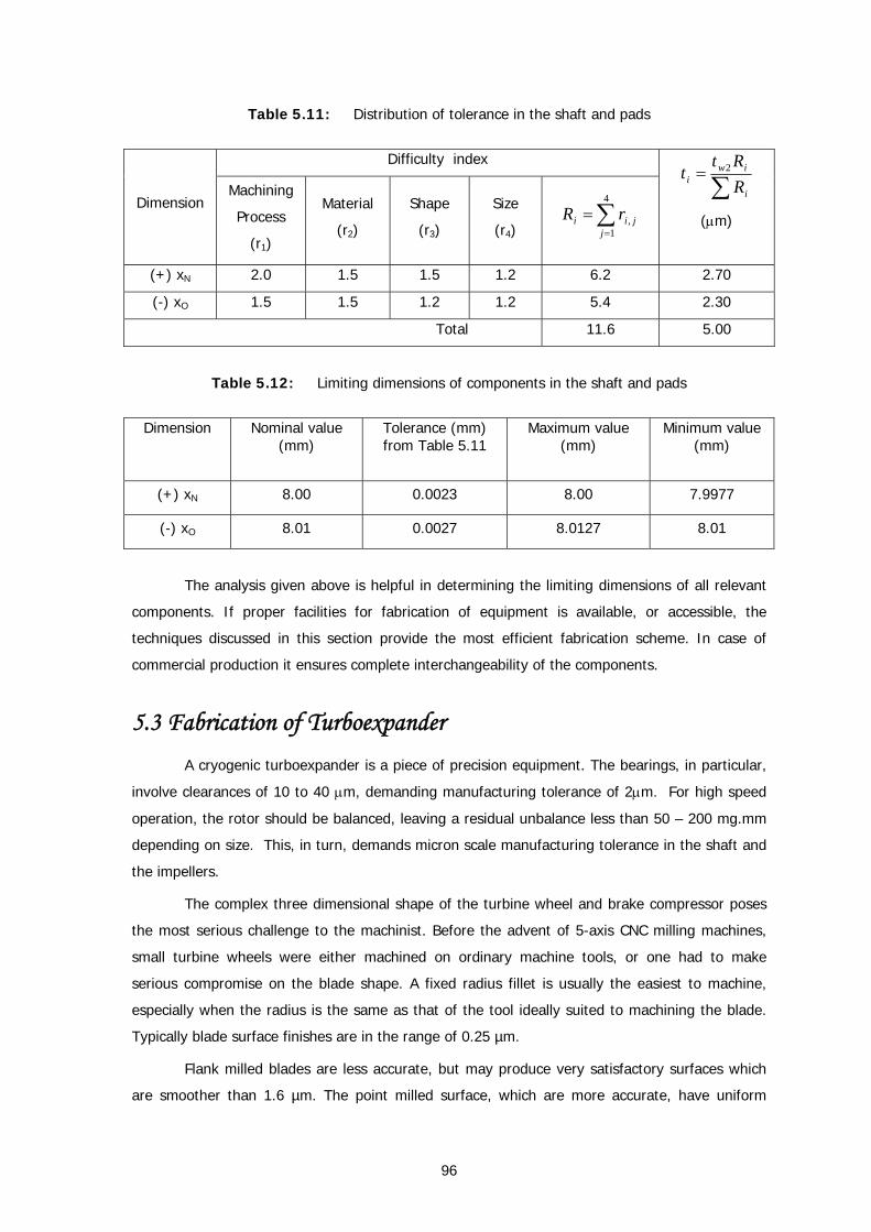
96

Table 5.11: Distribution of tolerance in the shaft and pads

Difficulty index

Dimension Machining

Process

(r1)

Material

(r2)

Shape

(r3)

Size

(r4) ∑=

=4

1,

jjii rR

∑=

i

iwi R

Rtt 2

(μm)

(+) xN 2.0 1.5 1.5 1.2 6.2 2.70

(-) xO 1.5 1.5 1.2 1.2 5.4 2.30

Total 11.6 5.00

Table 5.12: Limiting dimensions of components in the shaft and pads

Dimension Nominal value

(mm) Tolerance (mm) from Table 5.11

Maximum value (mm)

Minimum value (mm)

(+) xN 8.00 0.0023 8.00 7.9977

(-) xO 8.01 0.0027 8.0127 8.01

The analysis given above is helpful in determining the limiting dimensions of all relevant

components. If proper facilities for fabrication of equipment is available, or accessible, the

techniques discussed in this section provide the most efficient fabrication scheme. In case of

commercial production it ensures complete interchangeability of the components.

5.3 Fabrication of Turboexpander A cryogenic turboexpander is a piece of precision equipment. The bearings, in particular,

involve clearances of 10 to 40 μm, demanding manufacturing tolerance of 2μm. For high speed

operation, the rotor should be balanced, leaving a residual unbalance less than 50 – 200 mg.mm

depending on size. This, in turn, demands micron scale manufacturing tolerance in the shaft and

the impellers.

The complex three dimensional shape of the turbine wheel and brake compressor poses

the most serious challenge to the machinist. Before the advent of 5-axis CNC milling machines,

small turbine wheels were either machined on ordinary machine tools, or one had to make

serious compromise on the blade shape. A fixed radius fillet is usually the easiest to machine,

especially when the radius is the same as that of the tool ideally suited to machining the blade.

Typically blade surface finishes are in the range of 0.25 µm.

Flank milled blades are less accurate, but may produce very satisfactory surfaces which

are smoother than 1.6 µm. The point milled surface, which are more accurate, have uniform

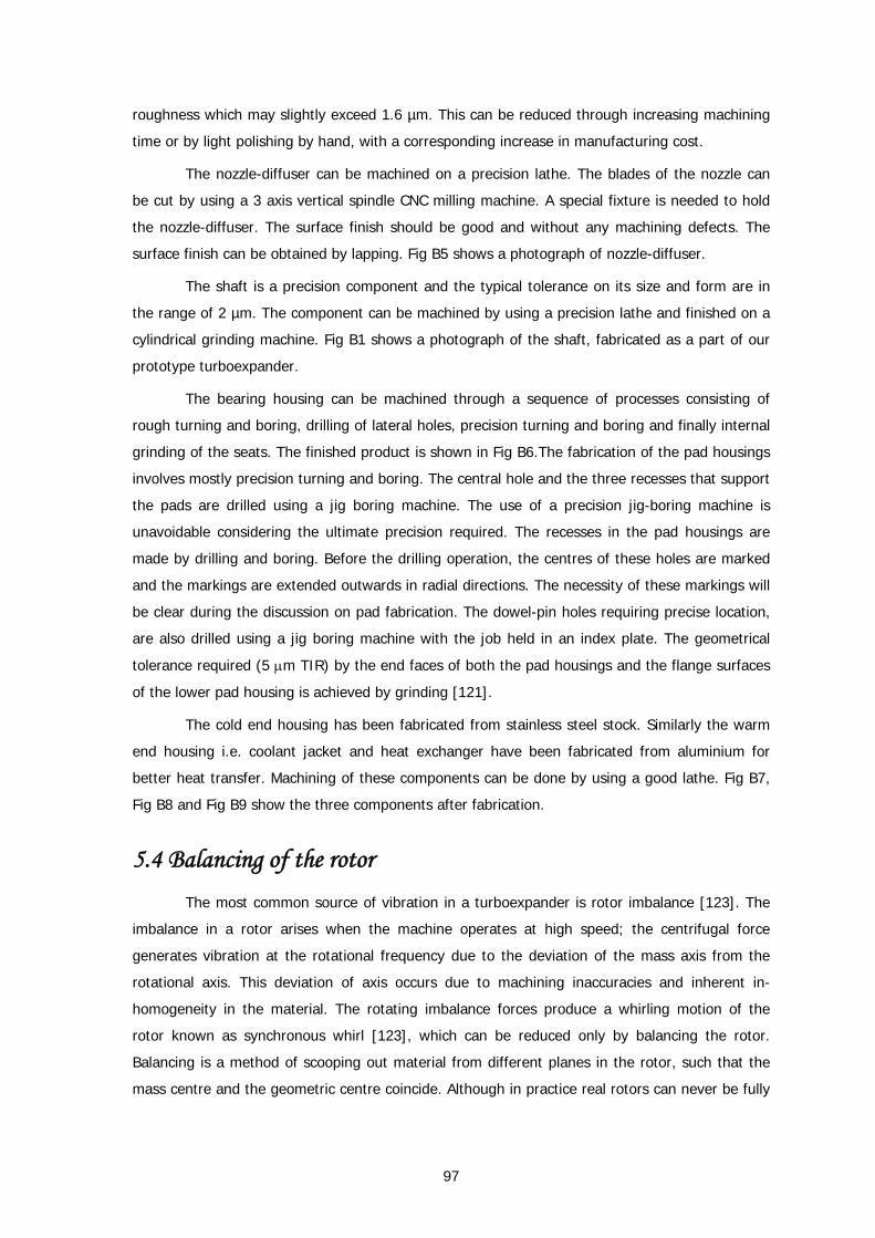
97

roughness which may slightly exceed 1.6 µm. This can be reduced through increasing machining

time or by light polishing by hand, with a corresponding increase in manufacturing cost.

The nozzle-diffuser can be machined on a precision lathe. The blades of the nozzle can

be cut by using a 3 axis vertical spindle CNC milling machine. A special fixture is needed to hold

the nozzle-diffuser. The surface finish should be good and without any machining defects. The

surface finish can be obtained by lapping. Fig B5 shows a photograph of nozzle-diffuser.

The shaft is a precision component and the typical tolerance on its size and form are in

the range of 2 µm. The component can be machined by using a precision lathe and finished on a

cylindrical grinding machine. Fig B1 shows a photograph of the shaft, fabricated as a part of our

prototype turboexpander.

The bearing housing can be machined through a sequence of processes consisting of

rough turning and boring, drilling of lateral holes, precision turning and boring and finally internal

grinding of the seats. The finished product is shown in Fig B6.The fabrication of the pad housings

involves mostly precision turning and boring. The central hole and the three recesses that support

the pads are drilled using a jig boring machine. The use of a precision jig-boring machine is

unavoidable considering the ultimate precision required. The recesses in the pad housings are

made by drilling and boring. Before the drilling operation, the centres of these holes are marked

and the markings are extended outwards in radial directions. The necessity of these markings will

be clear during the discussion on pad fabrication. The dowel-pin holes requiring precise location,

are also drilled using a jig boring machine with the job held in an index plate. The geometrical

tolerance required (5 μm TIR) by the end faces of both the pad housings and the flange surfaces

of the lower pad housing is achieved by grinding [121].

The cold end housing has been fabricated from stainless steel stock. Similarly the warm

end housing i.e. coolant jacket and heat exchanger have been fabricated from aluminium for

better heat transfer. Machining of these components can be done by using a good lathe. Fig B7,

Fig B8 and Fig B9 show the three components after fabrication.

5.4 Balancing of the rotor The most common source of vibration in a turboexpander is rotor imbalance [123]. The

imbalance in a rotor arises when the machine operates at high speed; the centrifugal force

generates vibration at the rotational frequency due to the deviation of the mass axis from the

rotational axis. This deviation of axis occurs due to machining inaccuracies and inherent in-

homogeneity in the material. The rotating imbalance forces produce a whirling motion of the

rotor known as synchronous whirl [123], which can be reduced only by balancing the rotor.

Balancing is a method of scooping out material from different planes in the rotor, such that the

mass centre and the geometric centre coincide. Although in practice real rotors can never be fully

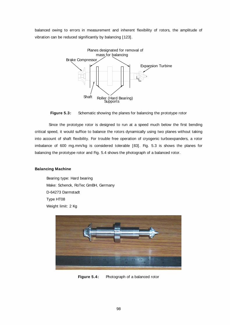
98

balanced owing to errors in measurement and inherent flexibility of rotors, the amplitude of

vibration can be reduced significantly by balancing [123].

Figure 5.3: Schematic showing the planes for balancing the prototype rotor

Since the prototype rotor is designed to run at a speed much below the first bending

critical speed, it would suffice to balance the rotors dynamically using two planes without taking

into account of shaft flexibility. For trouble free operation of cryogenic turboexpanders, a rotor

imbalance of 600 mg.mm/kg is considered tolerable [83]. Fig. 5.3 is shows the planes for

balancing the prototype rotor and Fig. 5.4 shows the photograph of a balanced rotor.

Balancing Machine

Bearing type: Hard bearing

Make: Schenck, RoTec GmBH, Germany

D-64273 Darmstadt

Type HT08

Weight limit: 2 Kg

Figure 5.4: Photograph of a balanced rotor

Shaft

Brake Compressor

Expansion Turbine

Roller (Hard Bearing)Supports

Planes designated for removal ofmass for balancing

99

Balancing Result of Shaft 1: Turbine side (Plane 1) Compressor side (Plane 2) Speed (rpm)

Initial Readings 27.9 mg at 14° 16.3 mg at 260° 2153

Before Grinding 3.19 mg at 262° 4.29 mg at 129° 2167

After Grinding 3.19 mg at 262° 4.29 mg at 129° 2167

Balancing Result of Shaft 2: Turbine side (Plane 1) Compressor side (Plane 2) Speed (rpm)

Initial Readings 6.93 mg at 337° 37.4 mg at 301° 2162

Before Grinding 7.37 mg at 332° 8.81 mg at 240° 2165

After Grinding 5.55 mg at 342° 9.75 mg at 89° 2165

5.5 Sequence of assembly Before beginning the assembly process, the components are given a final and thorough

checking. The gas inlet and outlet attachments to the bearing housing are tightly fastened for

supplying high-pressure gas and for discharging low pressure gas from the aerostatic thrust

bearings (if they are used). Similarly the high pressure and low pressure lines are also connected

to the compressor high pressure and low pressure lines respectively. The tubes are joined with

the cold end housing by welding. The flanges are finally faced off to remove any distortion due to

heating during welding. Once these steps are completed, the screws and O-rings are fitted to get

the final assembly of the prototype turboexpander. Fig. 5.5 shows the assembled Turboexpander.

The sequence of steps in the assembly process are given below:

⇒ Pads are pushed into their respective grooves in the pad housing.

⇒ End pad plates are tightly fastened by the screw to keep the pads in the proper position.

⇒ A Teflon make thermal insulator is placed at the bottom of the bearing housing.

⇒ Lower tilting pad journal bearing is placed on the thermal insulator.

⇒ The step of the tilting pad journal bearings are ensured to be in the direction of the shaft

collar.

⇒ The o-rings are pushed into their respective grooves in the thrust plate.

⇒ The spacer is placed in the centre position of the shaft collar.

⇒ The upper and lower thrust plates are pushed to the spacer from the two end of the

shaft.

⇒ The total unit of thrust plate and shaft are then to be kept in the bearing housing.

⇒ The upper journal bearing is placed on the upper thrust bearing in the bearing housing.

⇒ Two lock nuts are tightened at both the sides of turbine and compressor to keep the total

bearing unit in well balanced.

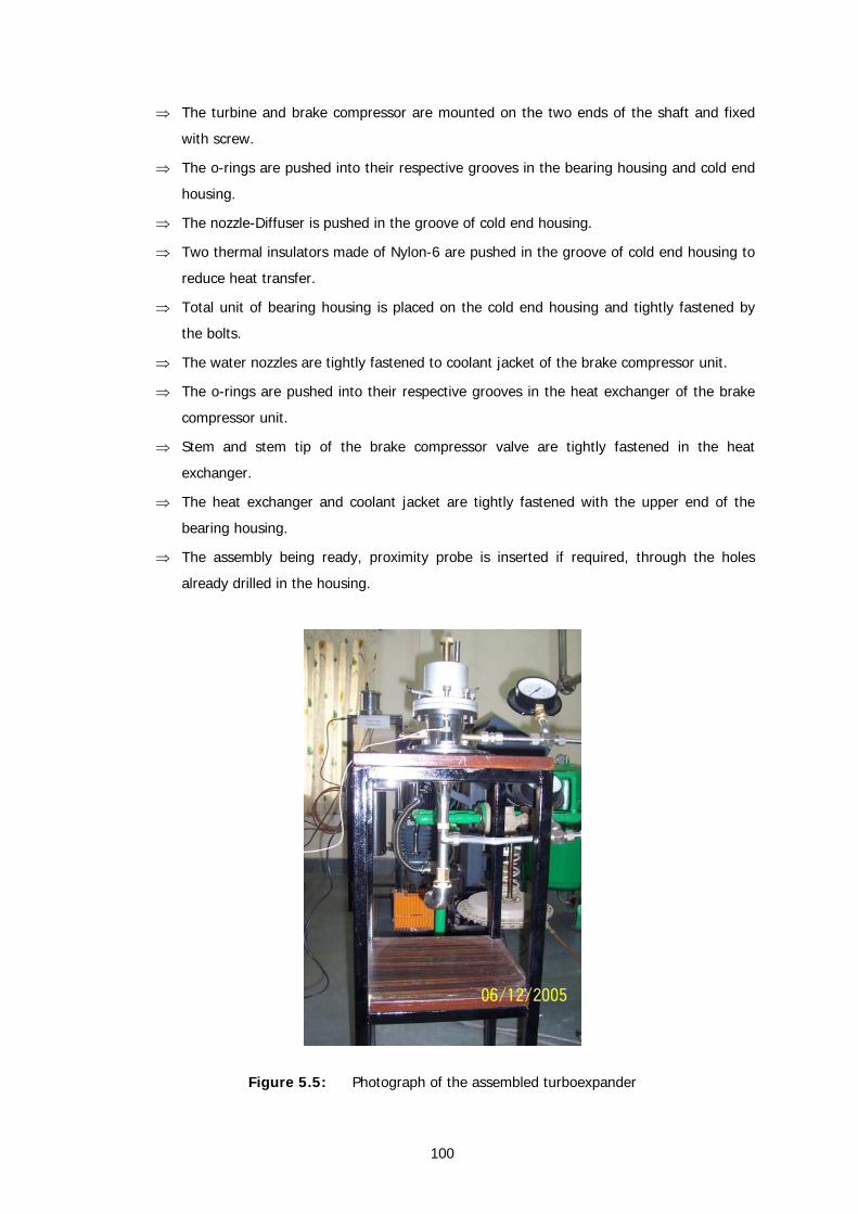
100

⇒ The turbine and brake compressor are mounted on the two ends of the shaft and fixed

with screw.

⇒ The o-rings are pushed into their respective grooves in the bearing housing and cold end

housing.

⇒ The nozzle-Diffuser is pushed in the groove of cold end housing.

⇒ Two thermal insulators made of Nylon-6 are pushed in the groove of cold end housing to

reduce heat transfer.

⇒ Total unit of bearing housing is placed on the cold end housing and tightly fastened by

the bolts.

⇒ The water nozzles are tightly fastened to coolant jacket of the brake compressor unit.

⇒ The o-rings are pushed into their respective grooves in the heat exchanger of the brake

compressor unit.

⇒ Stem and stem tip of the brake compressor valve are tightly fastened in the heat

exchanger.

⇒ The heat exchanger and coolant jacket are tightly fastened with the upper end of the

bearing housing.

⇒ The assembly being ready, proximity probe is inserted if required, through the holes

already drilled in the housing.

Figure 5.5: Photograph of the assembled turboexpander

101

5.6 Precautions during assembly and suggested changes Difficulties during assembly arose mostly from manufacturing inaccuracies, which can be

traced to the lack of proper machining facilities and other resource constraints. The difficulties

and the suggested changes during the assembly are briefly summarized as:

⇒ An extra attachment is needed to maintain the perpendicularity with the bearing housing

flange when the bearings and insulators are pushed into the bearing housing. As tight

clearance has to be maintained, a little inclination of the components may lead to

jamming of the rotor inside the bearing housing.

⇒ At the end pad plate ordinary circular holes are provided during manufacturing. Due to

this, the screw of the end pad plate has touched with the thrust plate. Later a counter

sunk hole was drilled on the end pad plate to alleviate this problem.

⇒ To maintain proper clearance between the turbine wheel and the nozzle, the help of the

length and hole size measuring instrument (Measurescope MM-22, NIKON, Japan) are

taken.

⇒ By taking the help of surface and cylindrical grinding facility it is being possible to push

the journal and thrust bearings inside the bearing housing.

⇒ Initially low pressure air from thrust bearing was not coming out to the atmosphere

because the connector was not connected properly upto the shaft collar. Later the

problem has been solved by making a connector which arrested the high pressure of the

bearing and allowed the low pressure to come out from the shaft collar to the

atmosphere.

Chapter 6

Experimental Performance

Study

Chapter VI

Experimental Performance Study

6.1 Turboexpander test rig The main motive of the present test is to study the performance of the turboexpander

under varying operating conditions. The process compressor takes air from the atmosphere

through a filter, compresses it and sends to a storage vessel, where it is maintained above the

required pressure of 0.6 MPa. We have tested two sets of turboexpanders, one having aerostatic

thrust bearings and the other aerodynamic thrust bearings. The schematic diagrams of the two

experimental test rigs are shown in Figures 6.1 and 6.2 respectively.

A high pressure air line originates from the vessel and branches into two lines; one is

connected to the inlet of the turbine and the other goes to the aerostatic thrust bearings. In the

test rig for the turbine with aerodynamic thrust bearings there is only one high-pressure line

connecting the vessel to the inlet of the turbine. In case of power shut down, normal or

abnormal, the turbine does not get the required supply of high pressure gas, but the rotor

continues to turn due to inertia. It may take several minutes for the rotational velocity to die

down completely. While the rotor is slowing down, it is necessary to maintain the bearing gas

supply to keep the rotor afloat. The bearing gas reservoir ensures these processes. The exhaust

gas from the turbine returns back to the inlet of the process compressor. There are pressure

gauges to measure the pressure at the vessel, inlet and outlet of the turbine and at the inlet to

the bearings.

A brake compressor installed on the same shaft as the turbine, operates in a closed

circuit. The gas is comes through the inlet pipe to the brake compressor and gets compressed.

The compressed gas leaving the brake compressor is cooled in a heat exchanger by a cooling

water supply and is fed back to the brake compressor. To reduce heat transfer to the cold end

housing, it is insulated by keeping inside a vacuum vessel.

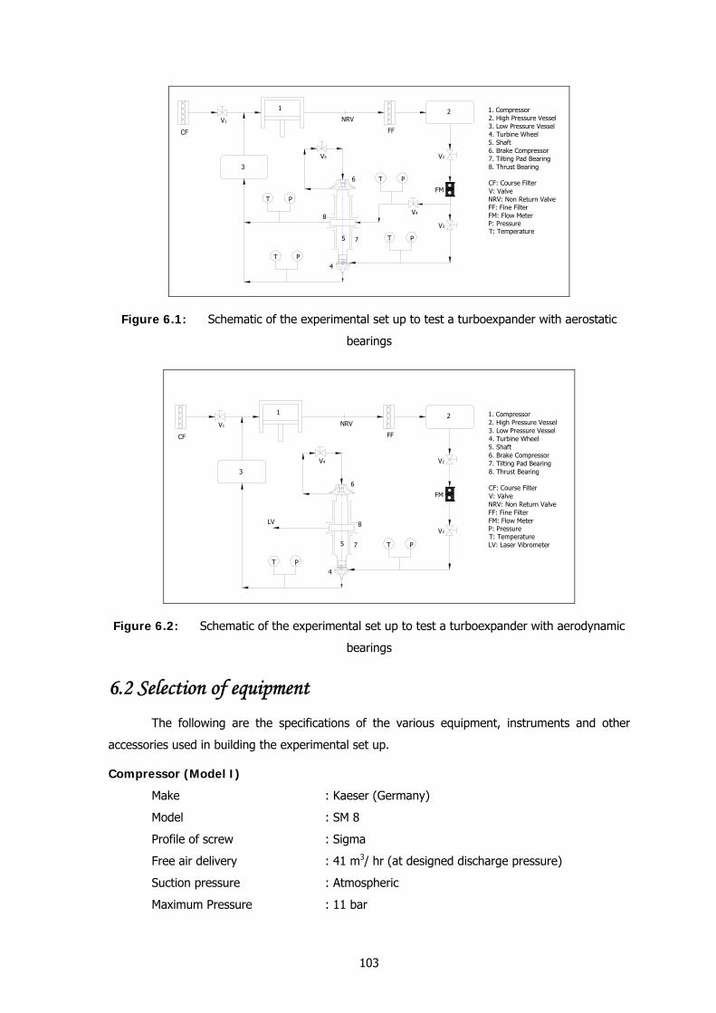
103

T P

8V4

PT

1. Compressor2. High Pressure Vessel3. Low Pressure Vessel4. Turbine Wheel5. Shaft6. Brake Compressor7. Tilting Pad Bearing8. Thrust Bearing

CF: Course FilterV: ValveNRV: Non Return ValveFF: Fine FilterFM: Flow MeterP: PressureT: Temperature

NRV

7

6

5

4

FM

3

21

V5

V3

V2

FFCF

V1

T P

PT

Figure 6.1: Schematic of the experimental set up to test a turboexpander with aerostatic

bearings

1. Compressor2. High Pressure Vessel3. Low Pressure Vessel4. Turbine Wheel5. Shaft6. Brake Compressor7. Tilting Pad Bearing8. Thrust Bearing

CF: Course FilterV: ValveNRV: Non Return ValveFF: Fine FilterFM: Flow MeterP: PressureT: TemperatureLV: Laser Vibrometer

LV

NRV

8

7

6

5

4

FM

3

21

V4

V3

V2

FFCF

V1

T P

PT

Figure 6.2: Schematic of the experimental set up to test a turboexpander with aerodynamic

bearings

6.2 Selection of equipment The following are the specifications of the various equipment, instruments and other

accessories used in building the experimental set up.

Compressor (Model I)

Make : Kaeser (Germany)

Model : SM 8

Profile of screw : Sigma

Free air delivery : 41 m3/ hr (at designed discharge pressure)

Suction pressure : Atmospheric

Maximum Pressure : 11 bar

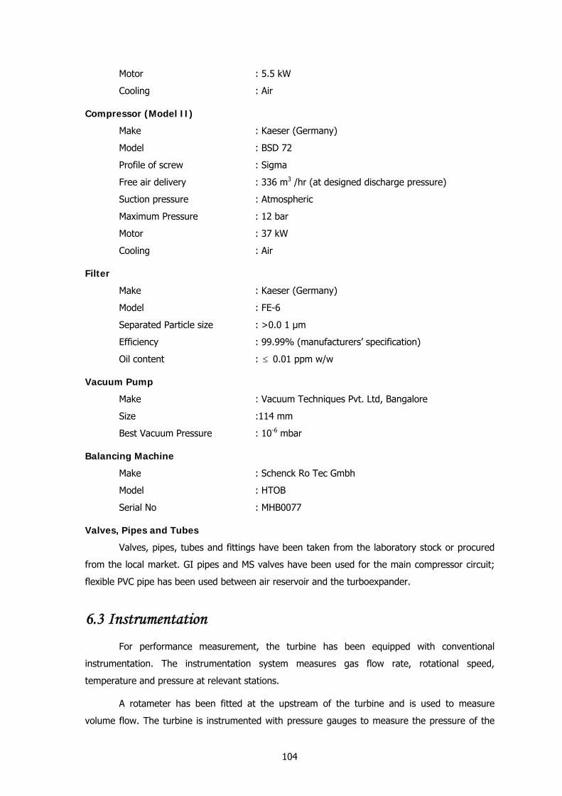
104

Motor : 5.5 kW

Cooling : Air

Compressor (Model II)

Make : Kaeser (Germany)

Model : BSD 72

Profile of screw : Sigma

Free air delivery : 336 m3 /hr (at designed discharge pressure)

Suction pressure : Atmospheric

Maximum Pressure : 12 bar

Motor : 37 kW

Cooling : Air

Filter

Make : Kaeser (Germany)

Model : FE-6

Separated Particle size : >0.0 1 μm

Efficiency : 99.99% (manufacturers’ specification)

Oil content : ≤ 0.01 ppm w/w

Vacuum Pump

Make : Vacuum Techniques Pvt. Ltd, Bangalore

Size :114 mm

Best Vacuum Pressure : 10-6 mbar

Balancing Machine

Make : Schenck Ro Tec Gmbh

Model : HTOB

Serial No : MHB0077

Valves, Pipes and Tubes

Valves, pipes, tubes and fittings have been taken from the laboratory stock or procured

from the local market. GI pipes and MS valves have been used for the main compressor circuit;

flexible PVC pipe has been used between air reservoir and the turboexpander.

6.3 Instrumentation For performance measurement, the turbine has been equipped with conventional

instrumentation. The instrumentation system measures gas flow rate, rotational speed,

temperature and pressure at relevant stations.

A rotameter has been fitted at the upstream of the turbine and is used to measure

volume flow. The turbine is instrumented with pressure gauges to measure the pressure of the

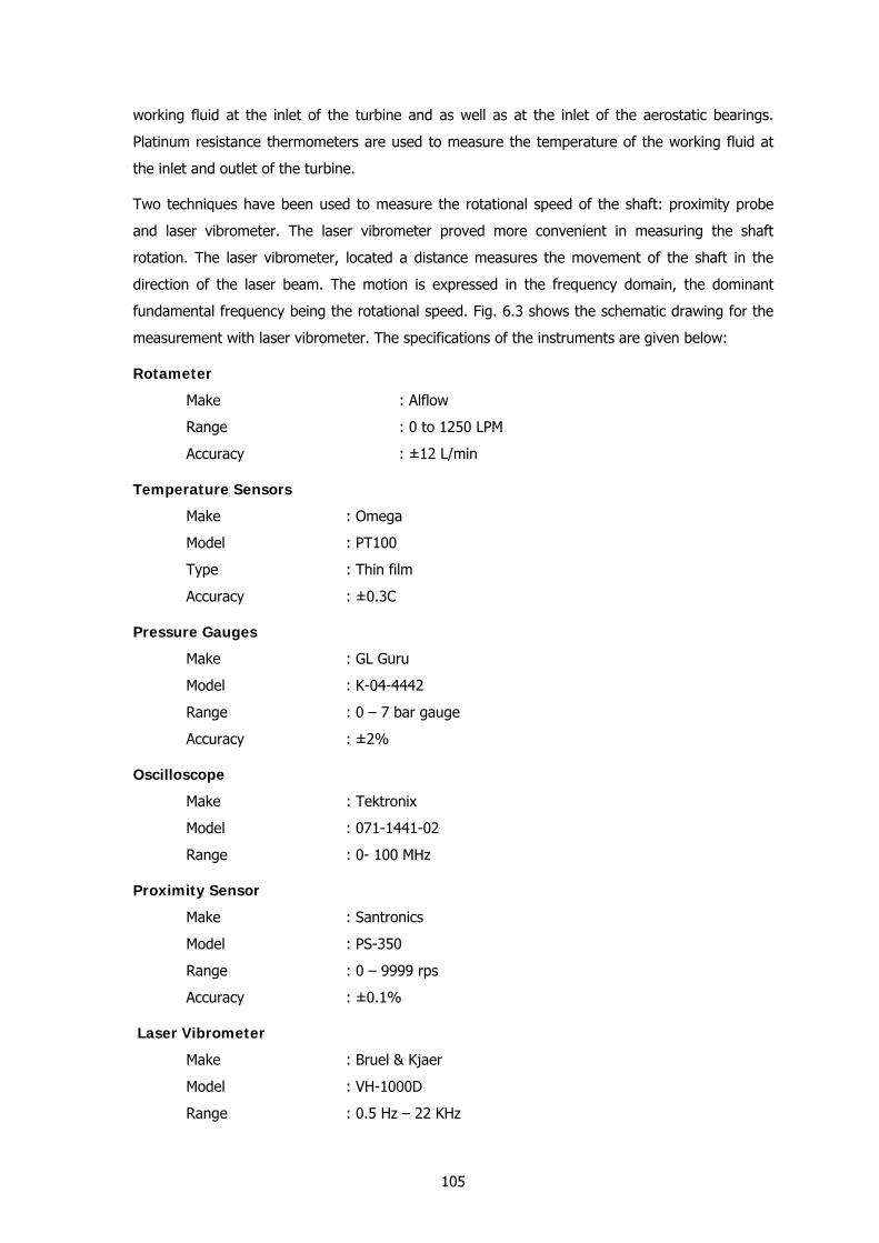
105

working fluid at the inlet of the turbine and as well as at the inlet of the aerostatic bearings.

Platinum resistance thermometers are used to measure the temperature of the working fluid at

the inlet and outlet of the turbine.

Two techniques have been used to measure the rotational speed of the shaft: proximity probe

and laser vibrometer. The laser vibrometer proved more convenient in measuring the shaft

rotation. The laser vibrometer, located a distance measures the movement of the shaft in the

direction of the laser beam. The motion is expressed in the frequency domain, the dominant

fundamental frequency being the rotational speed. Fig. 6.3 shows the schematic drawing for the

measurement with laser vibrometer. The specifications of the instruments are given below:

Rotameter

Make : Alflow

Range : 0 to 1250 LPM

Accuracy : ±12 L/min

Temperature Sensors

Make : Omega

Model : PT100

Type : Thin film

Accuracy : ±0.3C

Pressure Gauges

Make : GL Guru

Model : K-04-4442

Range : 0 – 7 bar gauge

Accuracy : ±2%

Oscilloscope

Make : Tektronix

Model : 071-1441-02

Range : 0- 100 MHz

Proximity Sensor

Make : Santronics

Model : PS-350

Range : 0 – 9999 rps

Accuracy : ±0.1%

Laser Vibrometer

Make : Bruel & Kjaer

Model : VH-1000D

Range : 0.5 Hz – 22 KHz

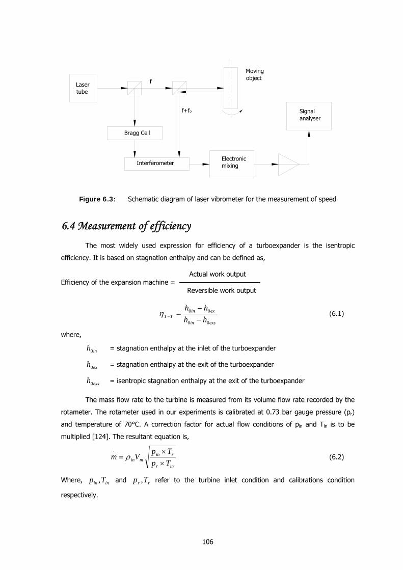
106

f+fD

f

Bragg Cell

InterferometerElectronic mixing

Signal analyser

Moving object

Laser tube

Figure 6.3: Schematic diagram of laser vibrometer for the measurement of speed

6.4 Measurement of efficiency

The most widely used expression for efficiency of a turboexpander is the isentropic

efficiency. It is based on stagnation enthalpy and can be defined as,

Actual work output Efficiency of the expansion machine = Reversible work output

exsin

exinTT hh

hh

00

00

−−

=−η (6.1)

where,

inh0 = stagnation enthalpy at the inlet of the turboexpander

exh0 = stagnation enthalpy at the exit of the turboexpander

exsh0 = isentropic stagnation enthalpy at the exit of the turboexpander

The mass flow rate to the turbine is measured from its volume flow rate recorded by the

rotameter. The rotameter used in our experiments is calibrated at 0.73 bar gauge pressure (pr)

and temperature of 70°C. A correction factor for actual flow conditions of pin and Tin is to be

multiplied [124]. The resultant equation is,

inr

rinmin Tp

TpVm

××

= ρ.

(6.2)

Where, inin Tp , and rr Tp , refer to the turbine inlet condition and calibrations condition

respectively.

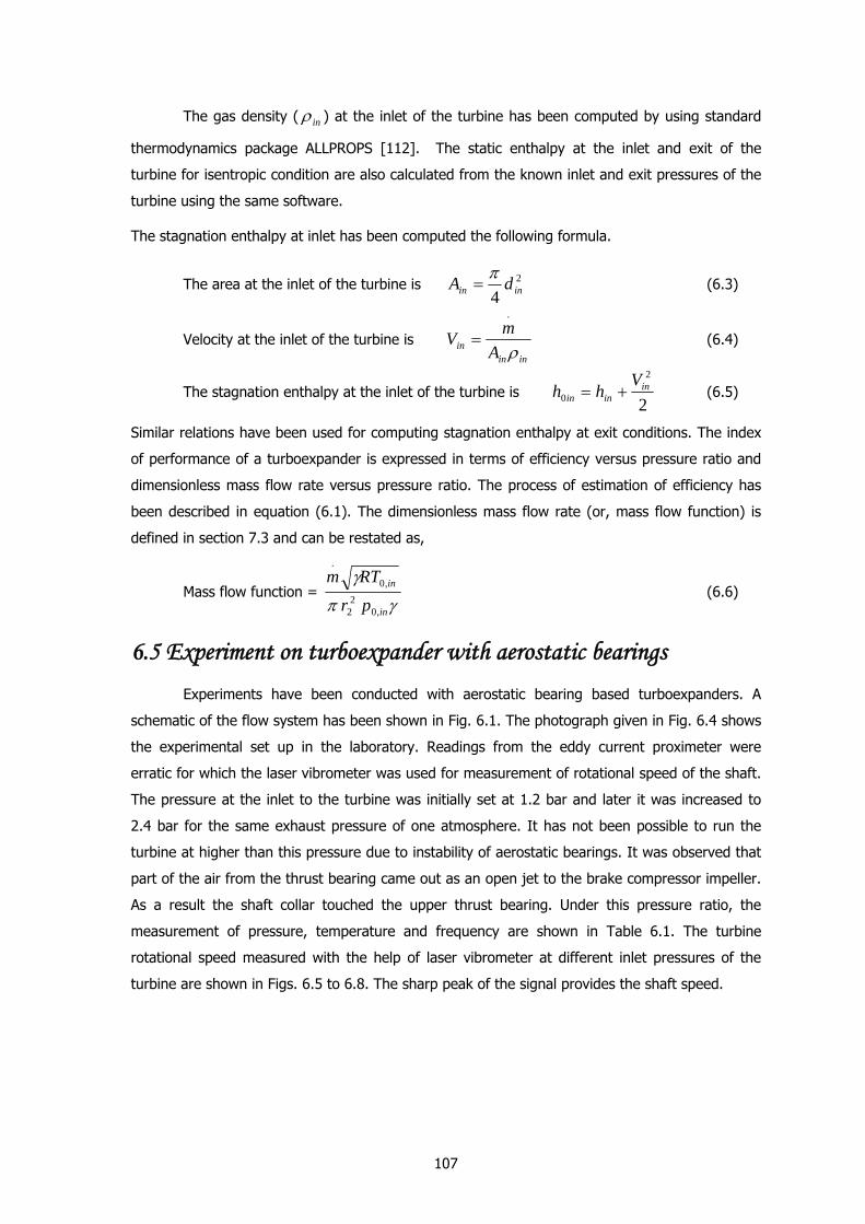
107

The gas density ( inρ ) at the inlet of the turbine has been computed by using standard

thermodynamics package ALLPROPS [112]. The static enthalpy at the inlet and exit of the

turbine for isentropic condition are also calculated from the known inlet and exit pressures of the

turbine using the same software.

The stagnation enthalpy at inlet has been computed the following formula.

The area at the inlet of the turbine is 2

4 inin dA π= (6.3)

Velocity at the inlet of the turbine is inin

in AmVρ

.

= (6.4)

The stagnation enthalpy at the inlet of the turbine is 2

2

0in

ininV

hh += (6.5)

Similar relations have been used for computing stagnation enthalpy at exit conditions. The index

of performance of a turboexpander is expressed in terms of efficiency versus pressure ratio and

dimensionless mass flow rate versus pressure ratio. The process of estimation of efficiency has

been described in equation (6.1). The dimensionless mass flow rate (or, mass flow function) is

defined in section 7.3 and can be restated as,

Mass flow function = γπ

γ

in

in

prRTm

,02

2

,0

.

(6.6)

6.5 Experiment on turboexpander with aerostatic bearings Experiments have been conducted with aerostatic bearing based turboexpanders. A

schematic of the flow system has been shown in Fig. 6.1. The photograph given in Fig. 6.4 shows

the experimental set up in the laboratory. Readings from the eddy current proximeter were

erratic for which the laser vibrometer was used for measurement of rotational speed of the shaft.

The pressure at the inlet to the turbine was initially set at 1.2 bar and later it was increased to

2.4 bar for the same exhaust pressure of one atmosphere. It has not been possible to run the

turbine at higher than this pressure due to instability of aerostatic bearings. It was observed that

part of the air from the thrust bearing came out as an open jet to the brake compressor impeller.

As a result the shaft collar touched the upper thrust bearing. Under this pressure ratio, the

measurement of pressure, temperature and frequency are shown in Table 6.1. The turbine

rotational speed measured with the help of laser vibrometer at different inlet pressures of the

turbine are shown in Figs. 6.5 to 6.8. The sharp peak of the signal provides the shaft speed.

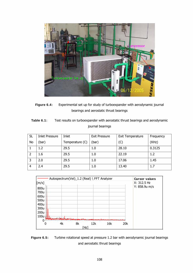
108

Figure 6.4: Experimental set up for study of turboexpander with aerodynamic journal

bearings and aerostatic thrust bearings

Table 6.1: Test results on turboexpander with aerostatic thrust bearings and aerodynamic

journal bearings

SL

No

Inlet Pressure

(bar)

Inlet

Temperature (C)

Exit Pressure

(bar)

Exit Temperature

(C)

Frequency

(KHz)

1 1.2 29.5 1.0 28.10 0.3125

2 1.6 29.5 1.0 22.19 1.2

3 2.0 29.5 1.0 17.06 1.45

4 2.4 29.5 1.0 13.40 1.7

0 4k 8k 12k 16k 20k[Hz]

0100u200u300u400u500u600u700u800u

[m/s]Cursor valuesX: 312.5 HzY: 858.9u m/s

Autospectrum(Vel)_1.2 (Real) \ FFT Analyzer

Figure 6.5: Turbine rotational speed at pressure 1.2 bar with aerodynamic journal bearings

and aerostatic thrust bearings

Turboexpander Set up

Compressor

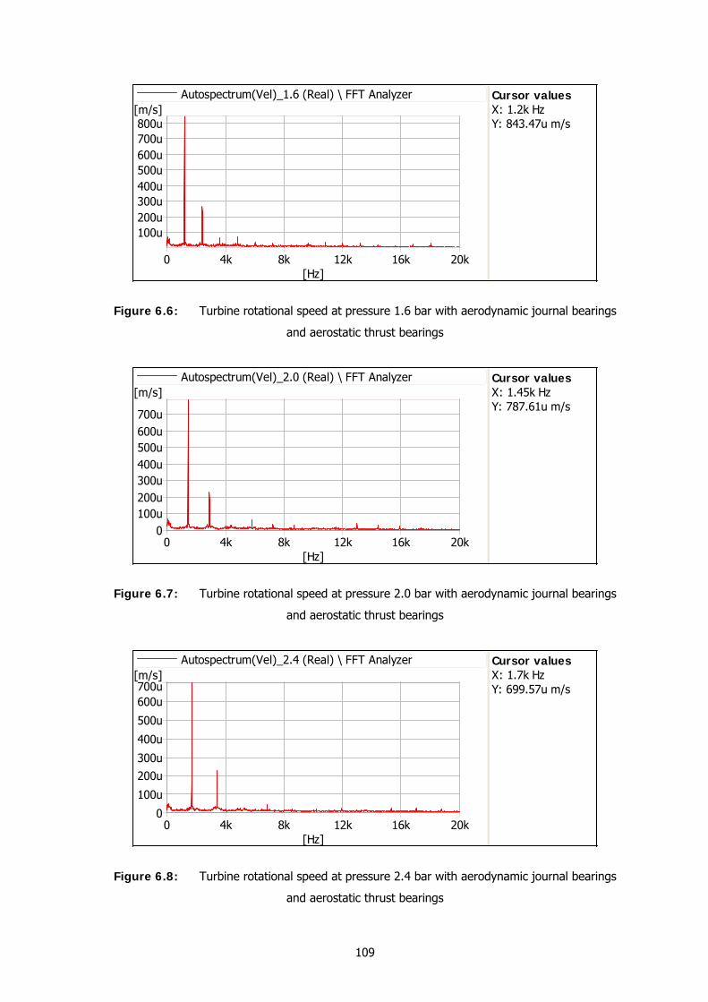
109

0 4k 8k 12k 16k 20k[Hz]

100u200u300u400u500u600u700u800u[m/s]

Cursor valuesX: 1.2k HzY: 843.47u m/s

Autospectrum(Vel)_1.6 (Real) \ FFT Analyzer

Figure 6.6: Turbine rotational speed at pressure 1.6 bar with aerodynamic journal bearings

and aerostatic thrust bearings

0 4k 8k 12k 16k 20k[Hz]

0100u200u300u400u500u600u700u

[m/s]Cursor valuesX: 1.45k HzY: 787.61u m/s

Autospectrum(Vel)_2.0 (Real) \ FFT Analyzer

Figure 6.7: Turbine rotational speed at pressure 2.0 bar with aerodynamic journal bearings

and aerostatic thrust bearings

0 4k 8k 12k 16k 20k[Hz]

0

100u

200u300u

400u

500u

600u700u[m/s]

Cursor valuesX: 1.7k HzY: 699.57u m/s

Autospectrum(Vel)_2.4 (Real) \ FFT Analyzer

Figure 6.8: Turbine rotational speed at pressure 2.4 bar with aerodynamic journal bearings

and aerostatic thrust bearings

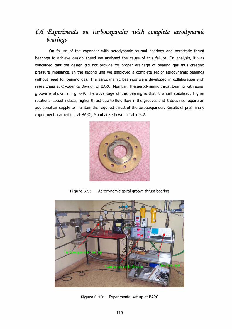
110

6.6 Experiments on turboexpander with complete aerodynamic bearings

On failure of the expander with aerodynamic journal bearings and aerostatic thrust

bearings to achieve design speed we analysed the cause of this failure. On analysis, it was

concluded that the design did not provide for proper drainage of bearing gas thus creating

pressure imbalance. In the second unit we employed a complete set of aerodynamic bearings

without need for bearing gas. The aerodynamic bearings were developed in collaboration with

researchers at Cryogenics Division of BARC, Mumbai. The aerodynamic thrust bearing with spiral

groove is shown in Fig. 6.9. The advantage of this bearing is that it is self stabilized. Higher

rotational speed induces higher thrust due to fluid flow in the grooves and it does not require an

additional air supply to maintain the required thrust of the turboexpander. Results of preliminary

experiments carried out at BARC, Mumbai is shown in Table 6.2.

Figure 6.9: Aerodynamic spiral groove thrust bearing

Figure 6.10: Experimental set up at BARC

Turboexpander Set up

Oscilloscope Temperature Indicator

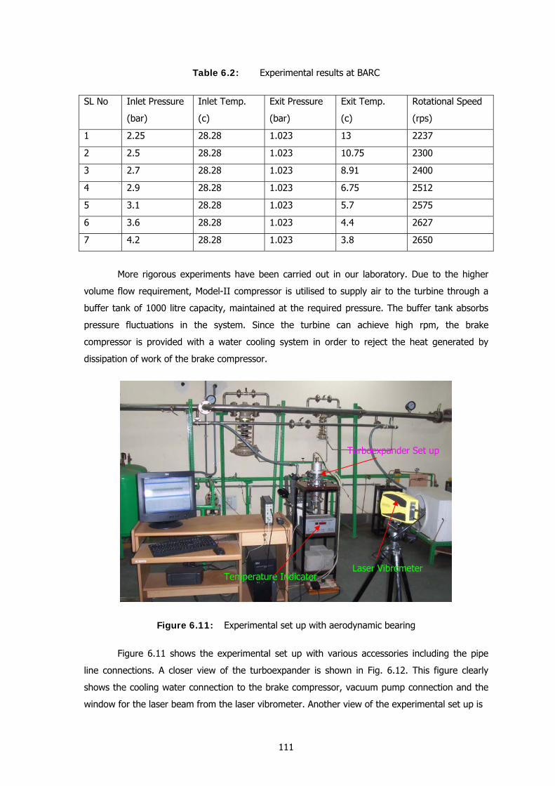
111

Table 6.2: Experimental results at BARC

SL No

Inlet Pressure

(bar)

Inlet Temp.

(c)

Exit Pressure

(bar)

Exit Temp.

(c)

Rotational Speed

(rps)

1 2.25 28.28 1.023 13 2237

2 2.5 28.28 1.023 10.75 2300

3 2.7 28.28 1.023 8.91 2400

4 2.9 28.28 1.023 6.75 2512

5 3.1 28.28 1.023 5.7 2575

6 3.6 28.28 1.023 4.4 2627

7 4.2 28.28 1.023 3.8 2650

More rigorous experiments have been carried out in our laboratory. Due to the higher

volume flow requirement, Model-II compressor is utilised to supply air to the turbine through a

buffer tank of 1000 litre capacity, maintained at the required pressure. The buffer tank absorbs

pressure fluctuations in the system. Since the turbine can achieve high rpm, the brake

compressor is provided with a water cooling system in order to reject the heat generated by

dissipation of work of the brake compressor.

Figure 6.11: Experimental set up with aerodynamic bearing

Figure 6.11 shows the experimental set up with various accessories including the pipe

line connections. A closer view of the turboexpander is shown in Fig. 6.12. This figure clearly

shows the cooling water connection to the brake compressor, vacuum pump connection and the

window for the laser beam from the laser vibrometer. Another view of the experimental set up is

Turboexpander Set up

Laser Vibrometer Temperature Indicator

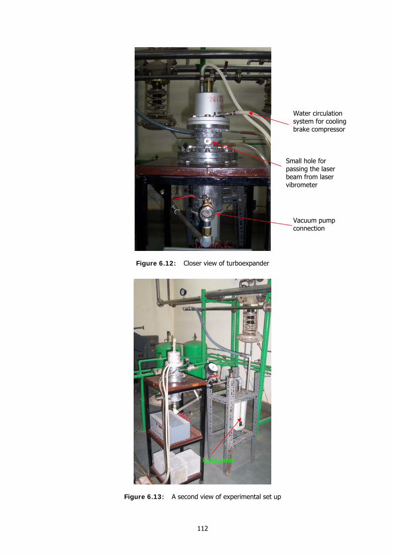
112

Figure 6.12: Closer view of turboexpander

Figure 6.13: A second view of experimental set up

Rotatmeter

Small hole for passing the laser beam from laser vibrometer

Water circulation system for cooling brake compressor

Vacuum pump connection

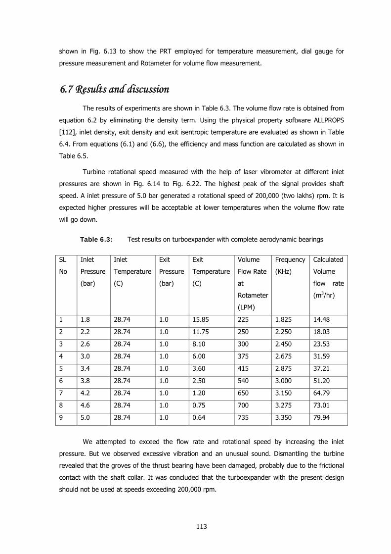
113

shown in Fig. 6.13 to show the PRT employed for temperature measurement, dial gauge for

pressure measurement and Rotameter for volume flow measurement.

6.7 Results and discussion The results of experiments are shown in Table 6.3. The volume flow rate is obtained from

equation 6.2 by eliminating the density term. Using the physical property software ALLPROPS

[112], inlet density, exit density and exit isentropic temperature are evaluated as shown in Table

6.4. From equations (6.1) and (6.6), the efficiency and mass function are calculated as shown in

Table 6.5.

Turbine rotational speed measured with the help of laser vibrometer at different inlet

pressures are shown in Fig. 6.14 to Fig. 6.22. The highest peak of the signal provides shaft

speed. A inlet pressure of 5.0 bar generated a rotational speed of 200,000 (two lakhs) rpm. It is

expected higher pressures will be acceptable at lower temperatures when the volume flow rate

will go down.

Table 6.3: Test results on turboexpander with complete aerodynamic bearings

SL

No

Inlet

Pressure

(bar)

Inlet

Temperature

(C)

Exit

Pressure

(bar)

Exit

Temperature

(C)

Volume

Flow Rate

at

Rotameter

(LPM)

Frequency

(KHz)

Calculated

Volume

flow rate

(m3/hr)

1 1.8 28.74 1.0 15.85 225 1.825 14.48

2 2.2 28.74 1.0 11.75 250 2.250 18.03

3 2.6 28.74 1.0 8.10 300 2.450 23.53

4 3.0 28.74 1.0 6.00 375 2.675 31.59

5 3.4 28.74 1.0 3.60 415 2.875 37.21

6 3.8 28.74 1.0 2.50 540 3.000 51.20

7 4.2 28.74 1.0 1.20 650 3.150 64.79

8 4.6 28.74 1.0 0.75 700 3.275 73.01

9 5.0 28.74 1.0 0.64 735 3.350 79.94

We attempted to exceed the flow rate and rotational speed by increasing the inlet

pressure. But we observed excessive vibration and an unusual sound. Dismantling the turbine

revealed that the groves of the thrust bearing have been damaged, probably due to the frictional

contact with the shaft collar. It was concluded that the turboexpander with the present design

should not be used at speeds exceeding 200,000 rpm.

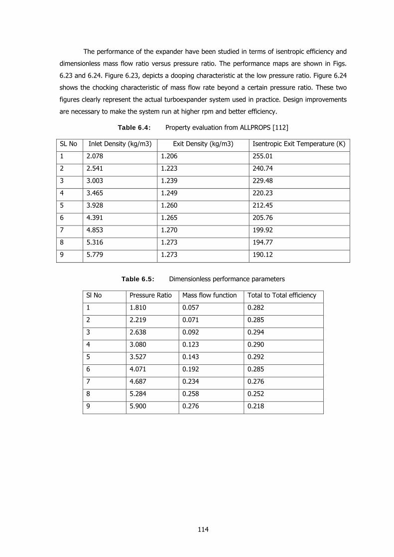
114

The performance of the expander have been studied in terms of isentropic efficiency and

dimensionless mass flow ratio versus pressure ratio. The performance maps are shown in Figs.

6.23 and 6.24. Figure 6.23, depicts a dooping characteristic at the low pressure ratio. Figure 6.24

shows the chocking characteristic of mass flow rate beyond a certain pressure ratio. These two

figures clearly represent the actual turboexpander system used in practice. Design improvements

are necessary to make the system run at higher rpm and better efficiency.

Table 6.4: Property evaluation from ALLPROPS [112] SL No Inlet Density (kg/m3) Exit Density (kg/m3) Isentropic Exit Temperature (K)

1 2.078 1.206 255.01

2 2.541 1.223 240.74

3 3.003 1.239 229.48

4 3.465 1.249 220.23

5 3.928 1.260 212.45

6 4.391 1.265 205.76

7 4.853 1.270 199.92

8 5.316 1.273 194.77

9 5.779 1.273 190.12

Table 6.5: Dimensionless performance parameters

Sl No Pressure Ratio Mass flow function Total to Total efficiency

1 1.810 0.057 0.282

2 2.219 0.071 0.285

3 2.638 0.092 0.294

4 3.080 0.123 0.290

5 3.527 0.143 0.292

6 4.071 0.192 0.285

7 4.687 0.234 0.276

8 5.284 0.258 0.252

9 5.900 0.276 0.218

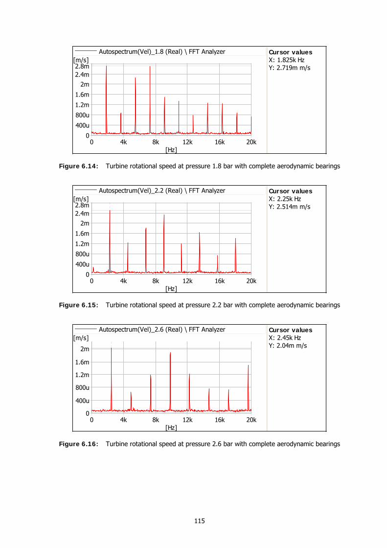
115

0 4k 8k 12k 16k 20k[Hz]

0

400u

800u

1.2m

1.6m

2m2.4m2.8m[m/s]

Cursor valuesX: 1.825k HzY: 2.719m m/s

Autospectrum(Vel)_1.8 (Real) \ FFT Analyzer

Figure 6.14: Turbine rotational speed at pressure 1.8 bar with complete aerodynamic bearings

0 4k 8k 12k 16k 20k[Hz]

0

400u

800u

1.2m

1.6m

2m2.4m2.8m[m/s]

Cursor valuesX: 2.25k HzY: 2.514m m/s

Autospectrum(Vel)_2.2 (Real) \ FFT Analyzer

Figure 6.15: Turbine rotational speed at pressure 2.2 bar with complete aerodynamic bearings

0 4k 8k 12k 16k 20k[Hz]

0

400u

800u

1.2m

1.6m

2m

[m/s]Cursor valuesX: 2.45k HzY: 2.04m m/s

Autospectrum(Vel)_2.6 (Real) \ FFT Analyzer

Figure 6.16: Turbine rotational speed at pressure 2.6 bar with complete aerodynamic bearings

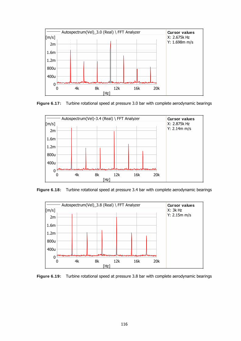
116

0 4k 8k 12k 16k 20k[Hz]

0

400u

800u

1.2m

1.6m

2m

[m/s]Cursor valuesX: 2.675k HzY: 1.698m m/s

Autospectrum(Vel)_3.0 (Real) \ FFT Analyzer

Figure 6.17: Turbine rotational speed at pressure 3.0 bar with complete aerodynamic bearings

0 4k 8k 12k 16k 20k[Hz]

0

400u

800u

1.2m

1.6m

2m

[m/s]Cursor valuesX: 2.875k HzY: 2.14m m/s

Autospectrum(Vel)-3.4 (Real) \ FFT Analyzer

Figure 6.18: Turbine rotational speed at pressure 3.4 bar with complete aerodynamic bearings

0 4k 8k 12k 16k 20k[Hz]

0

400u

800u

1.2m

1.6m

2m

[m/s]Cursor valuesX: 3k HzY: 2.15m m/s

Autospectrum(Vel)_3.8 (Real) \ FFT Analyzer

Figure 6.19: Turbine rotational speed at pressure 3.8 bar with complete aerodynamic bearings

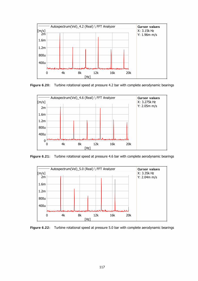
117

0 4k 8k 12k 16k 20k[Hz]

400u

800u

1.2m

1.6m

2m[m/s]

Cursor valuesX: 3.15k HzY: 1.96m m/s

Autospectrum(Vel)_4.2 (Real) \ FFT Analyzer

Figure 6.20: Turbine rotational speed at pressure 4.2 bar with complete aerodynamic bearings

0 4k 8k 12k 16k 20k[Hz]

0

400u

800u

1.2m

1.6m

2m

[m/s]Cursor valuesX: 3.275k HzY: 2.05m m/s

Autospectrum(Vel)_4.6 (Real) \ FFT Analyzer

Figure 6.21: Turbine rotational speed at pressure 4.6 bar with complete aerodynamic bearings

0 4k 8k 12k 16k 20k[Hz]

400u

800u

1.2m

1.6m

2m[m/s]

Cursor valuesX: 3.35k HzY: 2.04m m/s

Autospectrum(Vel)_5.0 (Real) \ FFT Analyzer

Figure 6.22: Turbine rotational speed at pressure 5.0 bar with complete aerodynamic bearings

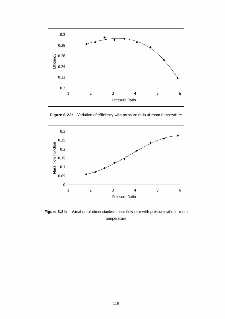
118

0.2

0.22

0.24

0.26

0.28

0.3

1 2 3 4 5 6

Pressure Ratio

Effic

ienc

y

Figure 6.23: Variation of efficiency with pressure ratio at room temperature

0

0.05

0.1

0.15

0.2

0.25

0.3

1 2 3 4 5 6

Pressure Ratio

Mas

s Fl

ow F

unct

ion

Figure 6.24: Variation of dimensionless mass flow rate with pressure ratio at room

temperature

Chapter VII

OFF DESIGN PERFORMANCE OF TURBEXPANDER

7.1 Introduction to performance analysis The foregoing chapters of this thesis has focussed on the design and development of

small cryogenic turboexpander system. It is also important for the designer to predict the

complete performance map of a machine so that alternative designs can be compared, assessed

and implemented. In addition, it is also important to predict the performance of our

turboexpander under off design conditions.

Depending on plant settings, the temperature, pressure and flow rate of a stream may

vary at the inlet to a turbine, albeit over a limited range. To predict the performance of a plant

under varying operating conditions, it is necessary to know the performance of the turbine under

arbitrarily prescribed specifications. This, in turn, necessitates the study of the performance of the

turbine at conditions away from the design point. Off-design performance calculations are also

helpful in choice of design modifications while building a new turbine with specifications

qualitatively similar, but quantitatively different from an existing one.

One of the easy but successful methods of analysing performance of a turbomachine is

the mean line or one-dimensional method pioneered by Whitfield and Baines [13]. A mean line

analysis is usually adopted since two and three-dimensional procedures are much more complex

and are not suitable for optimising the overall geometry. Mean line or one dimensional method is

routinely used for the design and analysis of radial turbines. They are very fast to compute and

require only a small amount of geometrical information. For these reasons they are extremely

useful in the initial stages of design before any detail of the blade geometry is fixed. Furthermore,

mean line methods are readily adapted to calculate off-design as well as design conditions, and

thus can be used to generate complete performance maps.

The prediction of the performance of a radial flow turbomachine generally involves the

analysis of the gas flow through the separate components used in its construction. Fig. 7.1 shows

the components of an expansion turbine along the fluid flow path. The general requirement of

the analytical procedure is to predict the component discharge conditions from known inlet

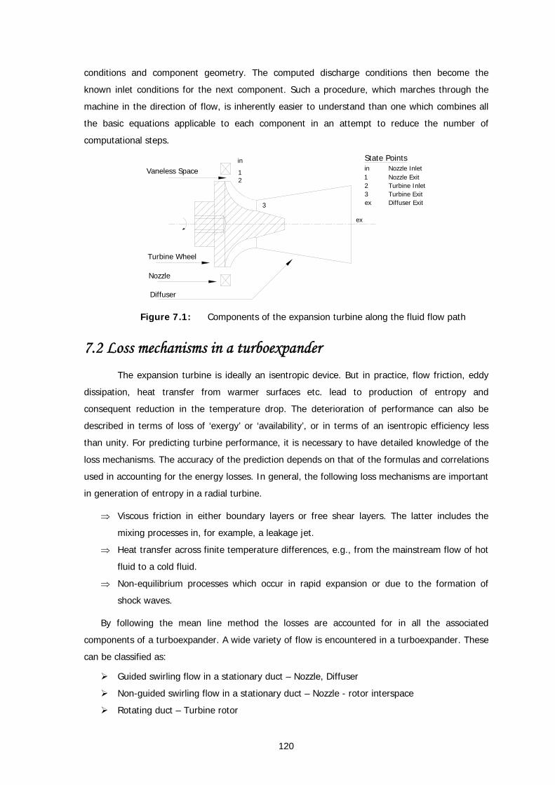
120

conditions and component geometry. The computed discharge conditions then become the

known inlet conditions for the next component. Such a procedure, which marches through the

machine in the direction of flow, is inherently easier to understand than one which combines all

the basic equations applicable to each component in an attempt to reduce the number of

computational steps.

Turbine Wheel

Diffuser

Nozzle

Vaneless Space 1

in

2

3

ex

State Pointsin Nozzle Inlet1 Nozzle Exit2 Turbine Inlet3 Turbine Exitex Diffuser Exit

Figure 7.1: Components of the expansion turbine along the fluid flow path

7.2 Loss mechanisms in a turboexpander The expansion turbine is ideally an isentropic device. But in practice, flow friction, eddy

dissipation, heat transfer from warmer surfaces etc. lead to production of entropy and

consequent reduction in the temperature drop. The deterioration of performance can also be

described in terms of loss of ‘exergy’ or ‘availability’, or in terms of an isentropic efficiency less

than unity. For predicting turbine performance, it is necessary to have detailed knowledge of the

loss mechanisms. The accuracy of the prediction depends on that of the formulas and correlations

used in accounting for the energy losses. In general, the following loss mechanisms are important

in generation of entropy in a radial turbine.

⇒ Viscous friction in either boundary layers or free shear layers. The latter includes the

mixing processes in, for example, a leakage jet.

⇒ Heat transfer across finite temperature differences, e.g., from the mainstream flow of hot

fluid to a cold fluid.

⇒ Non-equilibrium processes which occur in rapid expansion or due to the formation of

shock waves.

By following the mean line method the losses are accounted for in all the associated

components of a turboexpander. A wide variety of flow is encountered in a turboexpander. These

can be classified as:

Guided swirling flow in a stationary duct – Nozzle, Diffuser

Non-guided swirling flow in a stationary duct – Nozzle - rotor interspace

Rotating duct – Turbine rotor

121

A. Losses in the nozzle Radial inflow turbines usually have stator blades located in a flow field where the

meridional velocity is radially inward. The flow through the stator blades is highly accelerating

and, because of the decrease in radius the blade throat is close to, or even behind, the trailing

edge. Flow losses in the nozzle are associated with the high (near sonic) velocities generated in

the converging passages. They can be grouped under three separate heads.

i). Nozzle endwall loss This loss of exergy arises due to boundary layer friction and flow separation on surfaces

normal to the nozzle vanes i.e. on the floor and the ceiling of the nozzle passages.

ii). Trailing edge loss At the trailing edges of the nozzle blades, the gas undergoes sudden expansion, leading

to formation of eddies and consequent loss of exergy.

iii). Clearance loss In machines, where variable height or variable area nozzle is used, there is a flow of gas

through the clearance space around the attachments of the actuating mechanisms. The leakage

of process gas from high to low pressure leads to reduction of effective flow rate and consequent

fall in output power.

B. Losses in the vaneless space The flow between nozzle exit and rotor inlet is considered to be a free vortex flow of a

compressible fluid subjected to the resistance of skin friction. As a result, a strong velocity

gradient is generated leading to viscous losses.

C. Losses in the wheel

Loss mechanisms in turbomachinery passages are rarely independent of each other.

However, three terms “leakage loss”, “endwall loss” and “profile loss” are frequently used in

literature. Leakage losses are related to the leakage vortex that appears in unshrouded rotors. As

noted earlier, the interaction between leakage and secondary losses is strong, and it is not easy

to distinguish between these two. The relative sizes of these losses depend on the design of the

turbine; they can be of equal magnitude, each one of them amounting to a third stage loss.

Because of the twists and turns in the flow field, and the superimposed centrifugal force

field, the chance of flow separation in the wheel passage is high. A long flow passage with slow

turns leads to enhanced viscous drag, whereas short passages with sharp turns enhance the

chances of flow separation. There are four basic loss mechanisms operating in the wheel.

122

i). Passage losses

• Profile loss

Profile loss is the loss of exergy due to skin friction on the blade surface. As such it

depends on the area of the blade in contact with the fluid, the surface finish, and the Reynolds

number and the Mach number of the flow through the passage. All of these effects are governed

by the geometry of the airfoil. The radial inflow turbine has a three-dimensional blade profile and

the flow field generates forces on the blade surfaces due to centrifugal and Coriolis effects.

Losses due to boundary layer friction and separated flow on the blade surfaces are known as

profile losses. The extra loss arising at a trailing edge is also included in profile loss.

• Endwall loss

Endwall loss is also known as secondary loss. Secondary flows are vortices that occur as

a result of the boundary layers and the curvature of the passage, and cause some parts of the

fluid to move in directions other than the principal direction of flow. In the endwall boundary

layers the fluid velocities are lower than the mainstream, and the cross passage pressure gradient

causes the fluid to turn more sharply than at the center of the passage. However, the loss does

not arise directly from the secondary flow but is due to a combination of many factors. In a radial

flow turbine, where the boundary layer has a complex three-dimensional contour, it is very

difficult to predict these flows accurately. There are, however, reasonable empirical correlations

to describe these losses.

ii). Wheel clearance loss Clearance losses constitute a major source of inefficiency in turbine rotor blades. In a

turbomachine, there is a finite pressure difference between pressure and suction surfaces. In

fact, this difference of pressure accounts for loss of performance when fluid leaks through the

clearance gap rather than turning in the blade passage. It is because in doing so the fluid

produces no work. Designers always attempt to minimise the clearance gap. It should be kept in

mind that the gap depends on the cold clearance setting, modified by the elongation of the blade

under centrifugal stress and the differential thermal growth of the blade and casing. The actual

clearance therefore varies not only with operating condition, but also as a function of time

because dimensional changes do not happen instantaneously. This loss is known as clearance

loss.

iii). Rotor trailing edge loss The physically most meaningful expression of pressure losses due to trailing edge

blockage is in terms of the geometric blockage or trailing edge thickness or throat opening ratio

of a cascade. The trailing edge thickness is an important parameter in the design of turbine

blade, and has a significant influence on the overall performance. As the fluid leaves the rotor,

there is a sudden increase in the available cross section. This leads to creation of eddies and

123

dissipation of mechanical energy downstream of the rotor. The resulting loss of exergy is called

‘rotor trailing edge loss’.

iv). Incidence loss at Off-design conditions The aerodynamic design of a turbine is usually carried out in such a manner that

minimum loss occurs at the design point. This implies that the leading edges of the blades are

designed to match the direction of the incoming flow, a condition referred to as optimum or

design incidence. However, most turbines are also required to operate at conditions away from

their design point, and hence the inlet and outlet flow velocity vectors are mismatched with the

leading edge angle of the blades, causing additional losses that are commonly described as

incidence losses.

v). Disk friction loss In addition to the internal flow losses, as described above, external losses must be

considered. The external losses are those which give rise to increases in impeller discharge

stagnation enthalpy without any corresponding increase in pressure. These are classified as disc

friction loss and recirculation loss, but can also include any heat transfer from or to an external

source.

D. Losses in the diffuser The diffuser is a static, diverging channel. The losses are related to fluid friction in the

boundary layer and to flow separation.

E. Miscellaneous losses i). Friction loss This loss arises due to fluid friction on all parts of the machine, except for the blades and

the annulus boundaries. It is usually expressed in terms of the viscous torque on the rotating

disk.

ii). Exit kinetic energy loss The kinetic energy associated with gas leaving the system cannot be recovered; this loss

contributes to the overall deterioration of performance.

iii). Heat in-leak due to solid conduction In cryogenic turboexpanders, especially in small units operating at temperature of liquid

helium, heat conduction from the warm surfaces destroys a considerable amount of refrigeration

produced. For the turbine itself, it translates to a drop in isentropic efficiency.

iv). Seal Leakage Loss In turboexpanders using aerostatic bearings (and some times in aerodynamic bearings as

well) the system is vented to the atmosphere outside the bearings. A moving seal is provided

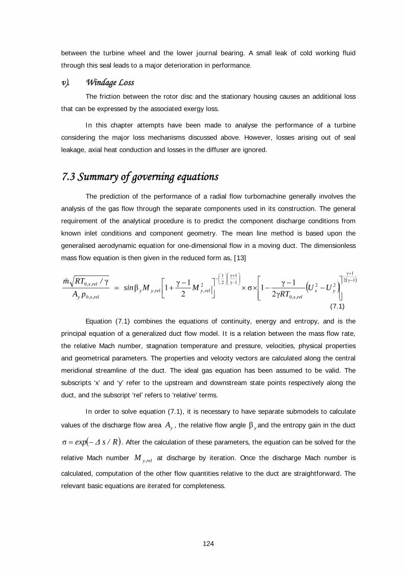
124

between the turbine wheel and the lower journal bearing. A small leak of cold working fluid

through this seal leads to a major deterioration in performance.

v). Windage Loss The friction between the rotor disc and the stationary housing causes an additional loss

that can be expressed by the associated exergy loss.

In this chapter attempts have been made to analyse the performance of a turbine

considering the major loss mechanisms discussed above. However, losses arising out of seal

leakage, axial heat conduction and losses in the diffuser are ignored.

7.3 Summary of governing equations The prediction of the performance of a radial flow turbomachine generally involves the

analysis of the gas flow through the separate components used in its construction. The general

requirement of the analytical procedure is to predict the component discharge conditions from

known inlet conditions and component geometry. The mean line method is based upon the

generalised aerodynamic equation for one-dimensional flow in a moving duct. The dimensionless

mass flow equation is then given in the reduced form as, [13]

( )( )1γ2

1γ

22

0

1γ1γ

21

2

0

0

γ21γ1σ

21γ1β

γ −+

⎟⎟⎠

⎞⎜⎜⎝

⎛−+

⎟⎠⎞

⎜⎝⎛−

⎥⎥⎦

⎤

⎢⎢⎣

⎡−

−−××⎥⎦

⎤⎢⎣⎡ −+= yx

rel,x,rel,yrel,yy

rel,x,y

rel,x, UURT

MMsinpA

/RTm&

(7.1)

Equation (7.1) combines the equations of continuity, energy and entropy, and is the

principal equation of a generalized duct flow model. It is a relation between the mass flow rate,

the relative Mach number, stagnation temperature and pressure, velocities, physical properties

and geometrical parameters. The properties and velocity vectors are calculated along the central

meridional streamline of the duct. The ideal gas equation has been assumed to be valid. The

subscripts ‘x’ and ‘y’ refer to the upstream and downstream state points respectively along the

duct, and the subscript ‘rel’ refers to ‘relative’ terms.

In order to solve equation (7.1), it is necessary to have separate submodels to calculate

values of the discharge flow area yA , the relative flow angle yβ and the entropy gain in the duct

( )R/sexp Δ−=σ . After the calculation of these parameters, the equation can be solved for the

relative Mach number rel,yM at discharge by iteration. Once the discharge Mach number is

calculated, computation of the other flow quantities relative to the duct are straightforward. The

relevant basic equations are iterated for completeness.

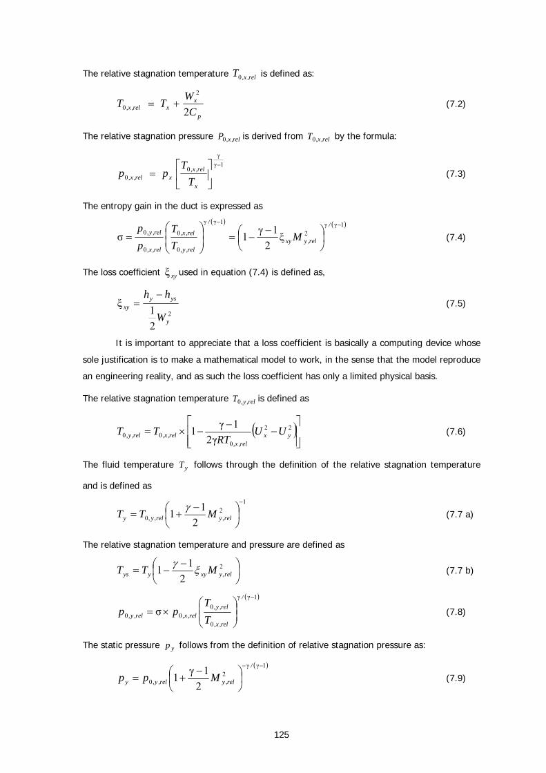
125

The relative stagnation temperature rel,x,T0 is defined as:

p

xxrel,x, C

WTT

2

2

0 += (7.2)

The relative stagnation pressure rel,x,P0 is derived from rel,x,T0 by the formula:

1γγ

00

−

⎥⎦

⎤⎢⎣

⎡=

x

rel,x,xrel,x, T

Tpp (7.3)

The entropy gain in the duct is expressed as

( ) ( )1γγ2

1γγ

0

0

0

0 ξ2

1γ1σ−−

⎟⎠⎞

⎜⎝⎛ −−=⎟

⎟⎠

⎞⎜⎜⎝

⎛=

/

rel,yxy

/

rel,y,

rel,x,

rel,x,

rel,y, MTT

pp

(7.4)

The loss coefficient xyξ used in equation (7.4) is defined as,

2

21

ξy

ysyxy

W

hh −= (7.5)

It is important to appreciate that a loss coefficient is basically a computing device whose

sole justification is to make a mathematical model to work, in the sense that the model reproduce

an engineering reality, and as such the loss coefficient has only a limited physical basis.

The relative stagnation temperature rel,y,T0 is defined as

( )⎥⎥⎦

⎤

⎢⎢⎣

⎡−

−−×= 22

000 γ2

1γ1 yxrel,x,

rel,x,rel,y, UURT

TT (7.6)

The fluid temperature yT follows through the definition of the relative stagnation temperature

and is defined as

12,,,0 2

11−

⎟⎠⎞

⎜⎝⎛ −+= relyrelyy MTT γ

(7.7 a)

The relative stagnation temperature and pressure are defined as

⎟⎠⎞

⎜⎝⎛ −−= 2

,211 relyxyyys MTT ξγ

(7.7 b)

( )1γγ

0

000 σ

−

⎟⎟⎠

⎞⎜⎜⎝

⎛×=

/

rel,x,

rel,y,rel,x,rel,y, T

Tpp (7.8)

The static pressure yp follows from the definition of relative stagnation pressure as:

( )1γγ

20 2

1γ1−−

⎟⎠⎞

⎜⎝⎛ −+=

/

rel,yrel,y,y Mpp (7.9)

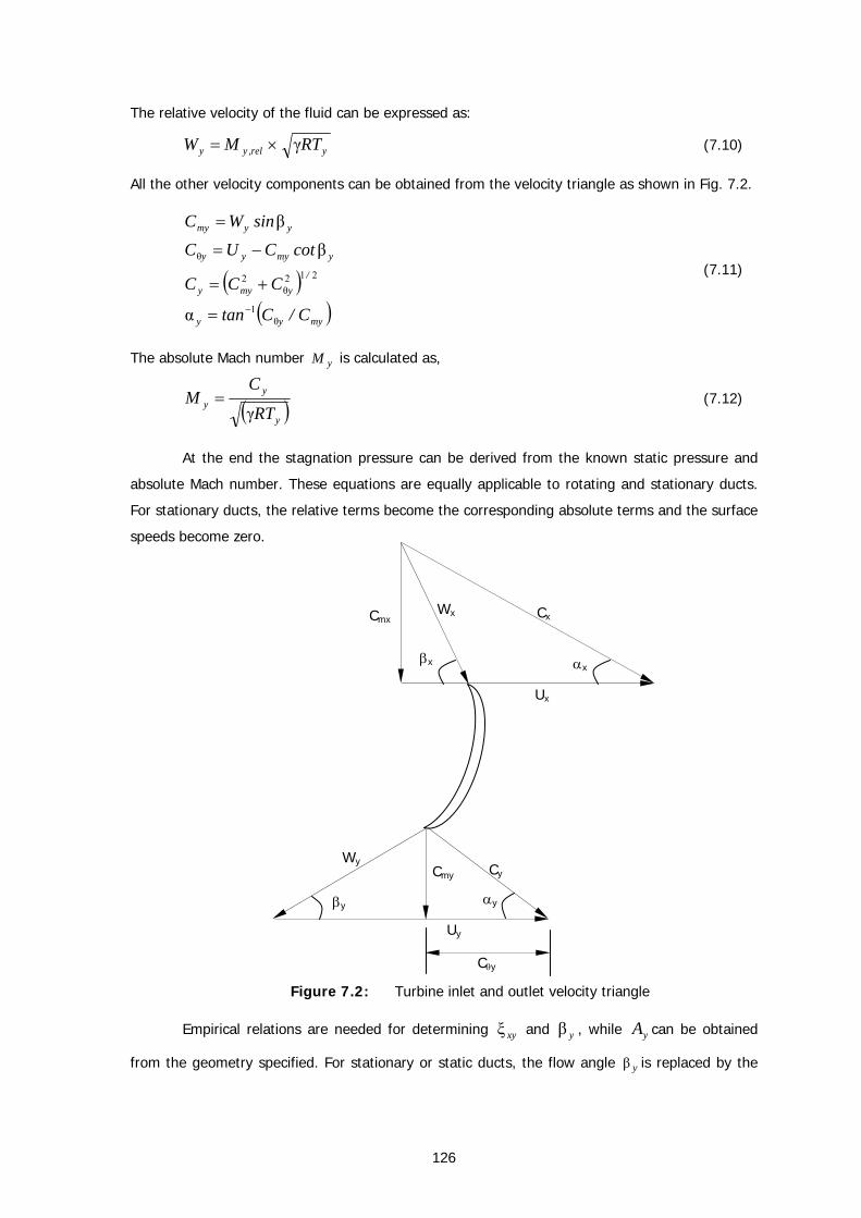
126

The relative velocity of the fluid can be expressed as:

yrel,yy RTMW γ×= (7.10)

All the other velocity components can be obtained from the velocity triangle as shown in Fig. 7.2.

( )( )myyy

/ymyy

ymyyy

yymy

C/Ctan

CCC

cotCUCsinWC

θ1

212θ

2

θ

α

ββ

−=

+=

−=

=

(7.11)

The absolute Mach number yM is calculated as,

( )y

yy RT

CM

γ= (7.12)

At the end the stagnation pressure can be derived from the known static pressure and

absolute Mach number. These equations are equally applicable to rotating and stationary ducts.

For stationary ducts, the relative terms become the corresponding absolute terms and the surface

speeds become zero.

Figure 7.2: Turbine inlet and outlet velocity triangle

Empirical relations are needed for determining xyξ and yβ , while yA can be obtained

from the geometry specified. For stationary or static ducts, the flow angle yβ is replaced by the

βy

βx αx

αy

Cx

Cy

Wx

Wy

Ux

Uy

Cmy

Cmx

Cθy

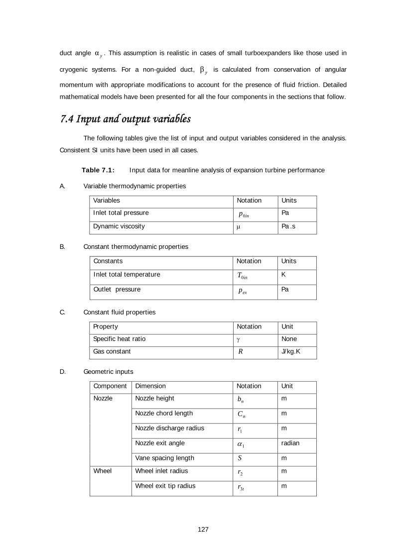
127

duct angle yα . This assumption is realistic in cases of small turboexpanders like those used in

cryogenic systems. For a non-guided duct, yβ is calculated from conservation of angular

momentum with appropriate modifications to account for the presence of fluid friction. Detailed

mathematical models have been presented for all the four components in the sections that follow.

7.4 Input and output variables The following tables give the list of input and output variables considered in the analysis.

Consistent SI units have been used in all cases.

Table 7.1: Input data for meanline analysis of expansion turbine performance

A. Variable thermodynamic properties

Variables Notation Units

Inlet total pressure inp0 Pa

Dynamic viscosity μ Pa .s

B. Constant thermodynamic properties

Constants Notation Units

Inlet total temperature inT0 K

Outlet pressure exp Pa

C. Constant fluid properties

Property Notation Unit

Specific heat ratio γ None

Gas constant R J/kg.K

D. Geometric inputs

Component Dimension Notation Unit

Nozzle height nb m

Nozzle chord length nC m

Nozzle discharge radius 1r m

Nozzle exit angle 1α radian

Nozzle

Vane spacing length S m

Wheel inlet radius 2r m Wheel

Wheel exit tip radius tr3 m

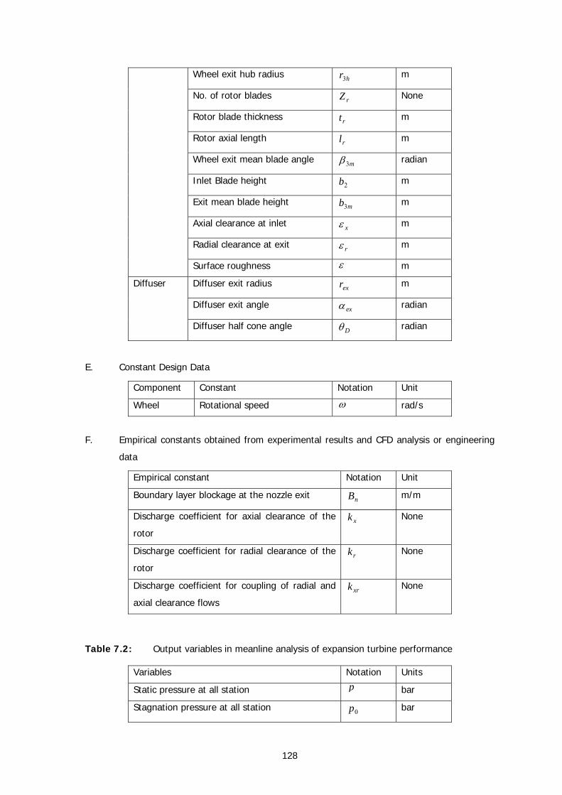
128

Wheel exit hub radius hr3 m

No. of rotor blades rZ None

Rotor blade thickness rt m

Rotor axial length rl m

Wheel exit mean blade angle m3β radian

Inlet Blade height 2b m

Exit mean blade height mb3 m

Axial clearance at inlet xε m

Radial clearance at exit rε m

Surface roughness ε m

Diffuser exit radius exr m

Diffuser exit angle exα radian

Diffuser

Diffuser half cone angle Dθ radian

E. Constant Design Data

Component Constant Notation Unit

Wheel Rotational speed ω rad/s

F. Empirical constants obtained from experimental results and CFD analysis or engineering

data

Empirical constant Notation Unit

Boundary layer blockage at the nozzle exit nB m/m

Discharge coefficient for axial clearance of the

rotor xk None

Discharge coefficient for radial clearance of the

rotor rk None

Discharge coefficient for coupling of radial and

axial clearance flows xrk None

Table 7.2: Output variables in meanline analysis of expansion turbine performance

Variables Notation Units

Static pressure at all station p bar

Stagnation pressure at all station 0p bar

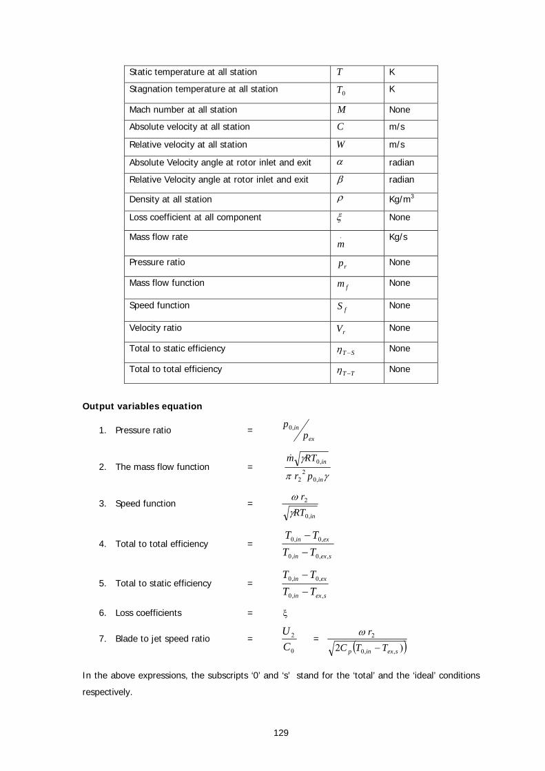
129

Static temperature at all station T K

Stagnation temperature at all station 0T K

Mach number at all station M None

Absolute velocity at all station C m/s

Relative velocity at all station W m/s

Absolute Velocity angle at rotor inlet and exit α radian

Relative Velocity angle at rotor inlet and exit β radian

Density at all station ρ Kg/m3

Loss coefficient at all component ξ None

Mass flow rate .m

Kg/s

Pressure ratio rp None

Mass flow function fm None

Speed function fS None

Velocity ratio rV None

Total to static efficiency ST −η None

Total to total efficiency TT −η None

Output variables equation

1. Pressure ratio = ex

inp

p ,0

2. The mass flow function = γπ

γ

in

in

pr

RTm

,02

2

,0&

3. Speed function = inRT

r

,0

2

γω

4. Total to total efficiency = sexin

exin

TTTT

,,0,0

,0,0

−

−

5. Total to static efficiency = sexin

exin

TTTT

,,0

,0,0

−

−

6. Loss coefficients = ξ

7. Blade to jet speed ratio = 0

2

CU

= ( ))2 ,,0

2

sexinp TTCr−

ω

In the above expressions, the subscripts ‘0’ and ‘s’ stand for the ‘total’ and the ‘ideal’ conditions

respectively.

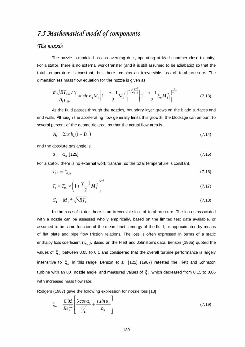
130

7.5 Mathematical model of components The nozzle

The nozzle is modeled as a converging duct, operating at Mach number close to unity.

For a stator, there is no external work transfer (and it is still assumed to be adiabatic) so that the

total temperature is constant, but there remains an irreversible loss of total pressure. The

dimensionless mass flow equation for the nozzle is given as

1γγ

21

1γ1γ

21

2111

01

0 ξ2

1γ12

1γ1αγ −+

−−

⎥⎦⎤

⎢⎣⎡ −−⎥⎦

⎤⎢⎣⎡ −+= MMMsin

pA/RTm

nin

in& (7.13)

As the fluid passes through the nozzles, boundary layer grows on the blade surfaces and

end walls. Although the accelerating flow generally limits this growth, the blockage can amount to

several percent of the geometric area, so that the actual flow area is

( )nn BbrA −= 1π2 11 (7.14)

and the absolute gas angle is,

nαα1 = [125] (7.15)

For a stator, there is no external work transfer, so the total temperature is constant.

in,, TT 010 = (7.16)

1

21101 2

1γ1−

⎟⎠⎞

⎜⎝⎛ −+×= MTT , (7.17)

111 γRT*MC = (7.18)

In the case of stator there is an irreversible loss of total pressure. The losses associated

with a nozzle can be assessed wholly empirically, based on the limited test data available, or

assumed to be some function of the mean kinetic energy of the fluid, or approximated by means

of flat plate and pipe flow friction relations. The loss is often expressed in terms of a static

enthalpy loss coefficient ( nξ ). Based on the Hiett and Johnston’s data, Benson (1965) quoted the

values of nξ between 0.05 to 0.1 and considered that the overall turbine performance is largely

insensitive to nξ in this range. Benson et al. [125] (1967) retested the Hiett and Johnston

turbine with an 80° nozzle angle, and measured values of nξ which decreased from 0.15 to 0.06

with increased mass flow rate.

Rodgers (1987) gave the following expression for nozzle loss [13]:

⎥⎥

⎦

⎤

⎢⎢

⎣

⎡+=

n.

bn b

sins

cs

cotRe

. 1120

αα3050ξ (7.19)

131

where

s = vane spacing

b = nozzle height

c = chord length

The isentropic temperature will be less than the actual static temperature due to loss and can be

expressed as:

⎟⎠⎞

⎜⎝⎛ −−×= 2

111 ξ2

1γ1 MTT ns (7.20)

( )1γγ

0

101

−

⎟⎟⎠

⎞⎜⎜⎝

⎛=

/

in

sin T

Tpp (7.21)

( )1γγ2

1101 21γ1

−

⎟⎠⎞

⎜⎝⎛ −+×=

/

Mpp (7.22)

( )111ρ RT/p= (7.23)

502

1

50

01

11 2

1γ1μμμ.

in

.

in MTT −

⎟⎠⎞

⎜⎝⎛ −+=⎟⎟

⎠

⎞⎜⎜⎝

⎛= (7.24)

The Reynolds number based on nozzle height and exit velocity is expressed as

1

11

μρ n

bbCRe = (7.25)

The independent variable in the calculation process is the exit Mach number 1M . For a

given value of 1M , equations (7.17) to (7.25) are solved in sequential order to obtain the values

of the thermodynamic variables and velocities at the exit of the nozzle. But to solve equation

(7.20), initially a guess value is taken for loss coefficient nξ from literature. Subsequently, nξ is

determined from the empirical equation (7.19) suggested by Whitfield and Baines [13].

Furthermore to get the exact value of nξ an iterative procedure is required. With well-machined

short nozzle vanes, the trailing edge losses can be neglected. Finally, after finding out all the

thermodynamic properties and the loss coefficient of the nozzle, the mass flow rate can be

determined from the equation (7.13).

The vaneless space

The vaneless space is modelled as an unguided converging duct, much like the vaneless

diffuser of a compressor and the bladeless nozzle of turbines, where unguided swirling flow

occurs. For a frictionless flow this leads to a free vortex condition. The losses arise due to viscous

forces and dissipation of eddies.

132

The initial guess value of 2C is taken as

( )2

112 r

r*CguessC = (7.26)

Being a static component, there is no external work transfer, so that the total temperature is

constant.

0102 TT =

pCCTT2

22

022 −= (7.27)

As the flow is unguided the angular momentum equation must be applied in order to

calculate the flow angle 2α . An empirical relationship has been assumed for the exit flow angle

α2 [13].

( )

mrrrcosCC

rr

cosCcosC f

&

122

2111

1

2

22

11 αρπ2αα −

+= (7.28)

where fC is skin friction co-efficient. It is expressed as [13]

250

1

121

μρ

240540

.

nf

b.

CC.C−

⎭⎬⎫

⎩⎨⎧

⎟⎠⎞

⎜⎝⎛ +

= (7.29)

The loss coefficient vsξ accounts for the frictional losses in a duct having hydraulic

diameter equal to the nozzle height and length equal to the radial distance between nozzle exit

and turbine inlet. The loss coefficient vsξ is expressed as

2

2

2121

224ξ ⎟⎟

⎠

⎞⎜⎜⎝

⎛ +⎟⎟⎠

⎞⎜⎜⎝

⎛ −=

CCC

brr

Cn

fvs (7.30)

p

vss C

CTT

2ξ 2

222 −= (7.31)

1γγ

01

2012

−

⎥⎦

⎤⎢⎣

⎡=

TT

pp s (7.32)

Using the above equations a new value of 2C is computed by applying continuity equations

222

22 αsinAp

RTmC

&= (7.33)

The area at the exit of the vaneless space being expressed as

( ) 222 π2 btZrA R−= (7.34)

To calculate 2α from equation (7.28) a guess value of 2C is assumed. A secant algorithm

is followed to arrive at a converged solution of 2C using an iterative procedure.

133

When the governing equations of the vaneless space are solved, state point ‘2’ is

completely defined. The following additional variables are computed to serve as input to the

solution of the equations governing the wheel.

1

2

02202

−γγ

⎟⎟⎠

⎞⎜⎜⎝

⎛=

TT

pp (7.35)

222

222 cos

sintanUC

C−αα

=β (7.36)

where 2U is the circumferential velocity at the inlet of the turbine wheel. It is expressed as:

22 ωrU = (7.37)

2222 βα eccossinCW = (7.38)

p

rel,, CWTT2

22

220 += (7.39)

1γγ

2

20220

−

⎟⎟⎠

⎞⎜⎜⎝

⎛=

TT

pp rel,,rel,, (7.40)

2

22ρ RT

p= (7.41)

22

22

22

22UWTCI p −+= (7.42)

In equation (7.42) 2I is the ‘rothalpy’ or relative enthalpy in a rotating frame. Its value remains

constant from entrance to exit.

The turbine wheel

Fluid friction, flow separation, impact, leakage and other dissipative phenomena occurring

in the wheel contribute the maximum towards the inefficiency of a turbomachine. In the case of a

rotor or impeller, the equation for flow conditions at a point applies as long as fluid properties

relative to the rotating component are consistently used, so that the absolute stagnation

temperature and pressure are replaced by relative stagnation values. The calculation of Mach

number is then the relative one. The simplest approach as stated by Futral and Wasserbauer

(1965) is that opt,xβ is considered to be equal to the rotor blade angle of 90° [13]. Therefore the

dimensionless mass flow equation for turbine wheel is expressed as:

( )( ) ( )

( )( )1γ2

1γ

23

22

02

1γ21γ

2333

023

02

γ21γ1

21γ1βσ

γ −+

−+−

⎥⎦

⎤⎢⎣

⎡−

−−⎥⎦

⎤⎢⎣⎡ −+= UU

RT*MMsin

pA/RTm

relrelrel

rel

rel& (7.43)

134

The entropy gain in the turbine wheel is expressed as

1γγ

23ξ

21γ1σ

−

⎥⎦⎤

⎢⎣⎡ −−= rel,R M (7.44)

The actual area at the outlet of the turbine wheel is,

( ) ( ) RRRhtht BeccostZrrrrA −−−−= 3332

32

33 βπ (7.45)

The second term in equation (7.45) accounts for the physical area blockage due to finite

trailing edge thickness. RB is the blockage due to profile and end-wall boundary layers and may

be obtained from experiments or from CFD studies. It is, however, expected to be a small

quantity and has been ignored in this analysis.

The circumferential velocities at the inlet and exit of the turbine wheel are expressed as

⎟⎠⎞

⎜⎝⎛ +

=2

ω 333

ht rrU (7.46)

( ) ( )

21

23

232

3

21γ1

21γ

⎥⎥⎥⎥

⎦

⎤

⎢⎢⎢⎢

⎣

⎡

−+

+−=

relM

UIW (7.47)

where the following thermodynamic relations are considered.

23

23

3 γ relRMW

T = (7.48)

⎟⎠⎞

⎜⎝⎛ −−= 2

333 ξ2

1γ1 relRs MTT (7.49)

1γγ

02

3023

−

⎟⎟⎠

⎞⎜⎜⎝

⎛=

rel

s

TT

pp (7.50)

3

33ρ RT

p= (7.51)

The loss terms

Incidence loss

This incidence model is based on the premise that the kinetic energy associated with the

change in relative tangential velocity is converted into internal energy of the working fluid. This

transformation leads to an increase in entropy. Under off-design conditions, the fluid approaches

the wheel at an angle different from the optimum value, thus increasing the exergy losses, and

can be expressed as [13]

( ) 2

3

,222 cos⎥⎦

⎤⎢⎣

⎡ −=

WW opt

I

ββξ (7.52)

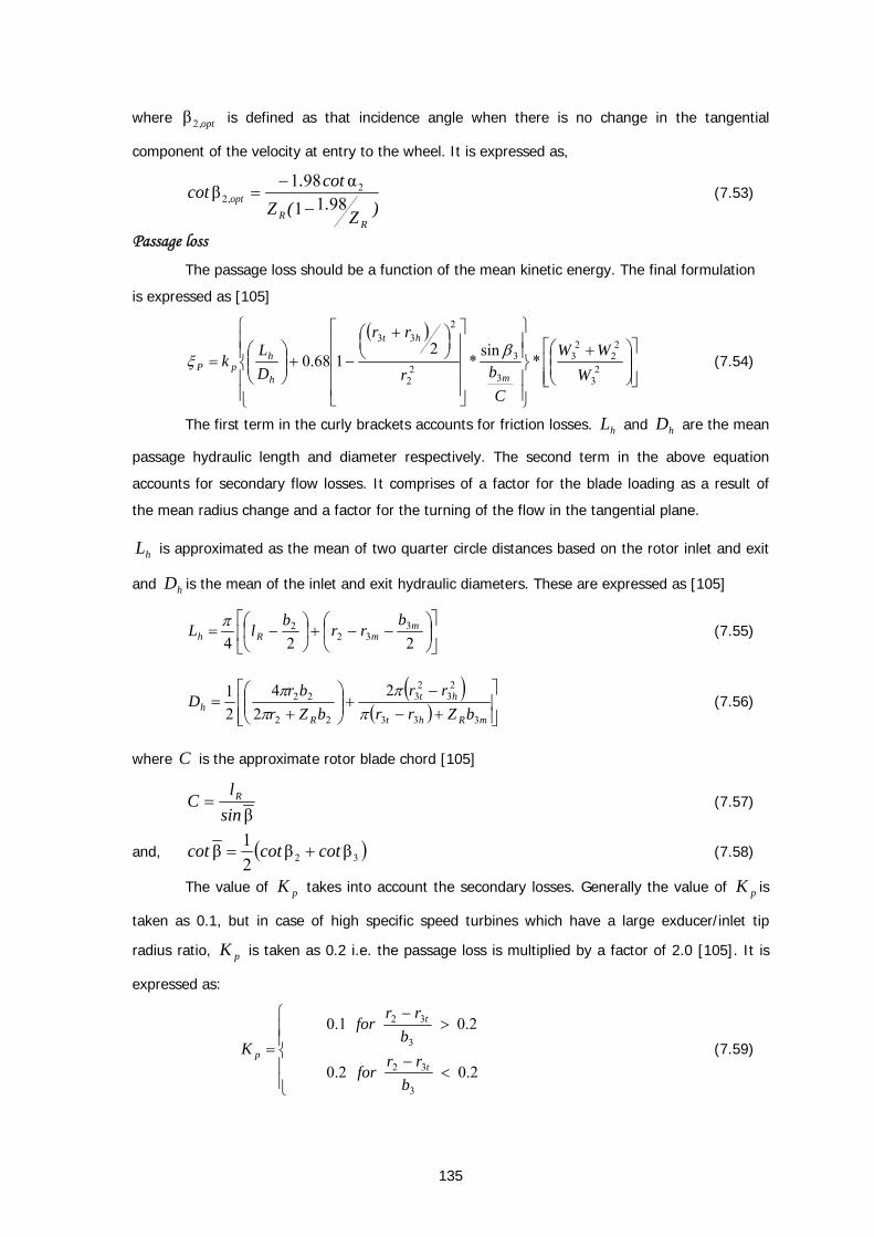
135

where opt,2β is defined as that incidence angle when there is no change in the tangential

component of the velocity at entry to the wheel. It is expressed as,

)Z.(Zcot.cot

RR

opt, 9811α981β 2

2−

−= (7.53)

Passage loss

The passage loss should be a function of the mean kinetic energy. The final formulation

is expressed as [105]

( )

⎥⎥⎦

⎤

⎢⎢⎣

⎡⎟⎟⎠

⎞⎜⎜⎝

⎛ +

⎪⎪⎭

⎪⎪⎬

⎫

⎪⎪⎩

⎪⎪⎨

⎧

⎥⎥⎥⎥

⎦

⎤

⎢⎢⎢⎢

⎣

⎡⎟⎠⎞⎜

⎝⎛ +

−+⎟⎟⎠

⎞⎜⎜⎝

⎛= 2

3

22

23

3

32

2

233

*sin

*2

168.0W

WW

Cbr

rr

DL

km

ht

h

hpP

βξ (7.54)

The first term in the curly brackets accounts for friction losses. hL and hD are the mean

passage hydraulic length and diameter respectively. The second term in the above equation

accounts for secondary flow losses. It comprises of a factor for the blade loading as a result of

the mean radius change and a factor for the turning of the flow in the tangential plane.

hL is approximated as the mean of two quarter circle distances based on the rotor inlet and exit

and hD is the mean of the inlet and exit hydraulic diameters. These are expressed as [105]

⎥⎦

⎤⎢⎣

⎡⎟⎠

⎞⎜⎝

⎛ −−+⎟⎠

⎞⎜⎝

⎛ −=2243

322 m

mRhb

rrb

lL π (7.55)

( )( ) ⎥

⎥⎦

⎤

⎢⎢⎣

⎡

+−−

+⎟⎟⎠

⎞⎜⎜⎝

⎛+

=mRht

ht

Rh bZrr

rrbZr

brD

333

23

23

22

22 22

421

ππ

ππ

(7.56)

where C is the approximate rotor blade chord [105]

βsinlC R= (7.57)

and, ( )32 ββ21β cotcotcot += (7.58)

The value of pK takes into account the secondary losses. Generally the value of pK is

taken as 0.1, but in case of high specific speed turbines which have a large exducer/inlet tip

radius ratio, pK is taken as 0.2 i.e. the passage loss is multiplied by a factor of 2.0 [105]. It is

expressed as:

⎪⎪⎩

⎪⎪⎨

⎧

<−

>−

=2.02.0

2.01.0

3

32

3

32

brr

for

brr

forK

t

t

p (7.59)

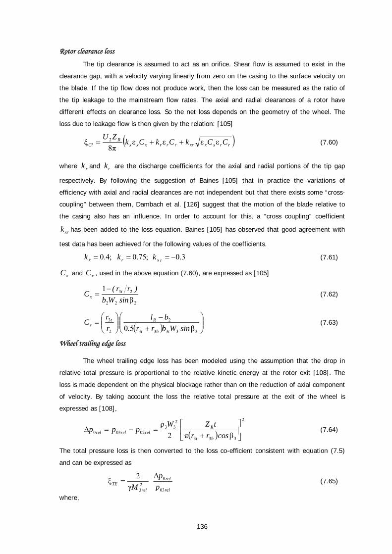
136

Rotor clearance loss

The tip clearance is assumed to act as an orifice. Shear flow is assumed to exist in the

clearance gap, with a velocity varying linearly from zero on the casing to the surface velocity on

the blade. If the tip flow does not produce work, then the loss can be measured as the ratio of

the tip leakage to the mainstream flow rates. The axial and radial clearances of a rotor have

different effects on clearance loss. So the net loss depends on the geometry of the wheel. The

loss due to leakage flow is then given by the relation: [105]

( )rrxxxrrrrxxxR

Cl CCkCkCkZU

εεεεπ8

ξ 2 ++= (7.60)

where xk and rk are the discharge coefficients for the axial and radial portions of the tip gap

respectively. By following the suggestion of Baines [105] that in practice the variations of

efficiency with axial and radial clearances are not independent but that there exists some “cross-

coupling” between them, Dambach et al. [126] suggest that the motion of the blade relative to

the casing also has an influence. In order to account for this, a “cross coupling” coefficient

xrk has been added to the loss equation. Baines [105] has observed that good agreement with

test data has been achieved for the following values of the coefficients.

3.0;75.0;4.0 −=== rxrx kkk (7.61)

xC and xC , used in the above equation (7.60), are expressed as [105]

222

23

β1

sinWb)rr(

C tx

−= (7.62)

( ) ⎟⎟⎠

⎞⎜⎜⎝

⎛+

−⎟⎟⎠

⎞⎜⎜⎝

⎛=

33333

2

2

3

β50 sinWbrr.bl

rr

Ctht

Rtr (7.63)

Wheel trailing edge loss

The wheel trailing edge loss has been modeled using the assumption that the drop in

relative total pressure is proportional to the relative kinetic energy at the rotor exit [108]. The

loss is made dependent on the physical blockage rather than on the reduction of axial component

of velocity. By taking account the loss the relative total pressure at the exit of the wheel is

expressed as [108],

( )

2

333

233

02030 βπ2ρ

⎥⎦

⎤⎢⎣

⎡+

=−=Δcosrr

tZWppp

ht

Rrelrelrel (7.64)

The total pressure loss is then converted to the loss co-efficient consistent with equation (7.5)

and can be expressed as

rel

rel

relTE p

pM 03

023γ

2ξΔ

= (7.65)

where,

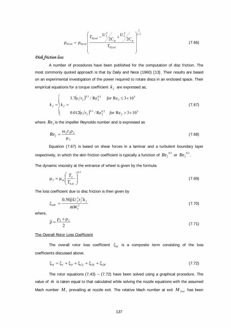
137

1γγ

02

23

22

02

0203

22−

⎟⎟⎟⎟

⎠

⎞

⎜⎜⎜⎜

⎝

⎛ +−=

rel

pprel

relrel TC

UC

UTpp (7.66)

Disk friction loss

A number of procedures have been published for the computation of disc friction. The

most commonly quoted approach is that by Daily and Nece (1960) [13]. Their results are based

on an experimental investigation of the power required to rotate discs in an enclosed space. Their

empirical equations for a torque coefficient fk are expressed as,

( )

( )⎪⎪⎩

⎪⎪⎨

⎧

×>∈

=×≤∈

=5

22.0

21.0

2

52

5.02

1.02

103ReRe/012.0

103ReRe/7.3

forr

kforr

k ff (7.67)

where 2Re is the impeller Reynolds number and is expressed as

2

2222 μ

ρω rRe = (7.68)

Equation (7.67) is based on shear forces in a laminar and a turbulent boundary layer

respectively, in which the skin friction coefficient is typically a function of 50

2.Re or

202

.Re .

The dynamic viscosity at the entrance of wheel is given by the formula:

50

0

22 μμ

.

in,in T

T⎟⎟⎠

⎞⎜⎜⎝

⎛= (7.69)

The loss coefficient due to disc friction is then given by

23

22

32ρ500

ξWm

krU. fDF &

= (7.70)

where,

2ρρρ 23 += (7.71)

The Overall Rotor Loss Coefficient

The overall rotor loss coefficient Rξ is a composite term consisting of the loss

coefficients discussed above.

DFTECLPIR ξξξξξξ ++++= (7.72)

The rotor equations (7.43) – (7.72) have been solved using a graphical procedure. The

value of m& is taken equal to that calculated while solving the nozzle equations with the assumed

Mach number 1M prevailing at nozzle exit. The relative Mach number at exit relM 3 has been

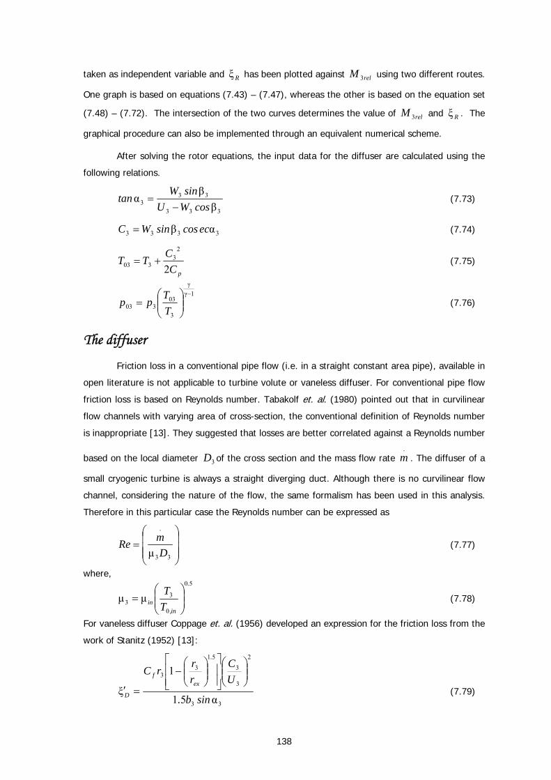
138

taken as independent variable and Rξ has been plotted against relM 3 using two different routes.

One graph is based on equations (7.43) – (7.47), whereas the other is based on the equation set

(7.48) – (7.72). The intersection of the two curves determines the value of relM 3 and Rξ . The

graphical procedure can also be implemented through an equivalent numerical scheme.

After solving the rotor equations, the input data for the diffuser are calculated using the

following relations.

333

333 β

βα

cosWUsinW

tan−

= (7.73)

3333 αβ eccossinWC = (7.74)

pCCTT2

23

303 += (7.75)

1γγ

3

03303

−

⎟⎟⎠

⎞⎜⎜⎝

⎛=

TT

pp (7.76)

The diffuser

Friction loss in a conventional pipe flow (i.e. in a straight constant area pipe), available in

open literature is not applicable to turbine volute or vaneless diffuser. For conventional pipe flow

friction loss is based on Reynolds number. Tabakolf et. al. (1980) pointed out that in curvilinear

flow channels with varying area of cross-section, the conventional definition of Reynolds number

is inappropriate [13]. They suggested that losses are better correlated against a Reynolds number

based on the local diameter 3D of the cross section and the mass flow rate .

m . The diffuser of a

small cryogenic turbine is always a straight diverging duct. Although there is no curvilinear flow

channel, considering the nature of the flow, the same formalism has been used in this analysis.

Therefore in this particular case the Reynolds number can be expressed as

⎟⎟⎟

⎠

⎞

⎜⎜⎜

⎝

⎛=

.

DmRe

33μ (7.77)

where, 50

0

33 μμ

.

in,in T

T⎟⎟⎠

⎞⎜⎜⎝

⎛= (7.78)

For vaneless diffuser Coppage et. al. (1956) developed an expression for the friction loss from the

work of Stanitz (1952) [13]:

33

2

3

3

51

33

α51

1

ξsinb.

UC

rr

rC.

exf

D

⎟⎟⎠

⎞⎜⎜⎝

⎛

⎥⎥⎦

⎤

⎢⎢⎣

⎡⎟⎟⎠

⎞⎜⎜⎝

⎛−

=′ (7.79)

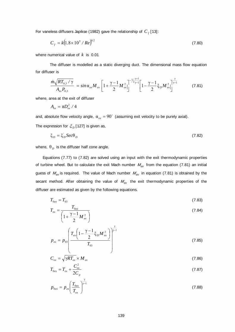
139

For vaneless diffusers Japikse (1982) gave the relationship of fC [13]:

( ) 2051081 .f Re/.kC ×= (7.80)

where numerical value of k is 0.01

The diffuser is modelled as a static diverging duct. The dimensional mass flow equation

for diffuser is

1γγ

21γ1γ

21

2

30

30 ξ2

1γ12

1γ1αγ −−

+−

⎥⎦⎤

⎢⎣⎡ −−⎥⎦

⎤⎢⎣⎡ −+= exDexexex

,ex

, MMMsinPA

/RTm& (7.81)

where, area at the exit of diffuser

4π 2 /DA exex =

and, absolute flow velocity angle, o90α =ex (assuming exit velocity to be purely axial).

The expression for Dξ [127] is given as,

D'DD Secθξξ = (7.82)

where, Dθ is the diffuser half cone angle.

Equations (7.77) to (7.82) are solved using an input with the exit thermodynamic properties

of turbine wheel. But to calculate the exit Mach number exM from the equation (7.81) an initial

guess of exM is required. The value of Mach number exM in equation (7.81) is obtained by the

secant method. After obtaining the value of exM the exit thermodynamic properties of the

diffuser are estimated as given by the following equations.

030 TT ex = (7.83)

⎟⎠⎞

⎜⎝⎛ −+

=2

0

21γ1 ex

exex

M

TT (7.84)

1γγ

03

2

03

ξ2

1γ1−

⎟⎟⎟⎟

⎠

⎞

⎜⎜⎜⎜

⎝

⎛⎟⎠⎞

⎜⎝⎛ −−

=T

MTpp

exDex

ex (7.85)

exexex MRTC ×= γ (7.86)

p

exexex C

CTT

2

2

0 += (7.87)

1γγ

00

−

⎟⎟⎠

⎞⎜⎜⎝

⎛=

ex

exexex T

Tpp (7.88)

140

γ

1γ

0

000

−

⎟⎟⎠

⎞⎜⎜⎝

⎛=

in

exinexs p

pTT (7.89)

7.6 Solution of governing equations The set of equations (7.13) to (7.89) constitutes the governing equations of a

turboexpander under off-design conditions. It contains both implicit and explicit equations. The

primary input to a design or analysis process are the pressure and total temperature at inlet and

exit, fluid properties and geometry of the turbine. Unfortunately, these parameters do not appear

explicitly in some of the equations. To address to this problem, the Mach number at exit of the

nozzle, 1M is taken as the independent variable. The mass flow rate and input conditions are

computed from this input data. The downstream states are computed subsequently. The details

of the computation process are given in the computational flow chart as described in Fig. 7.3.

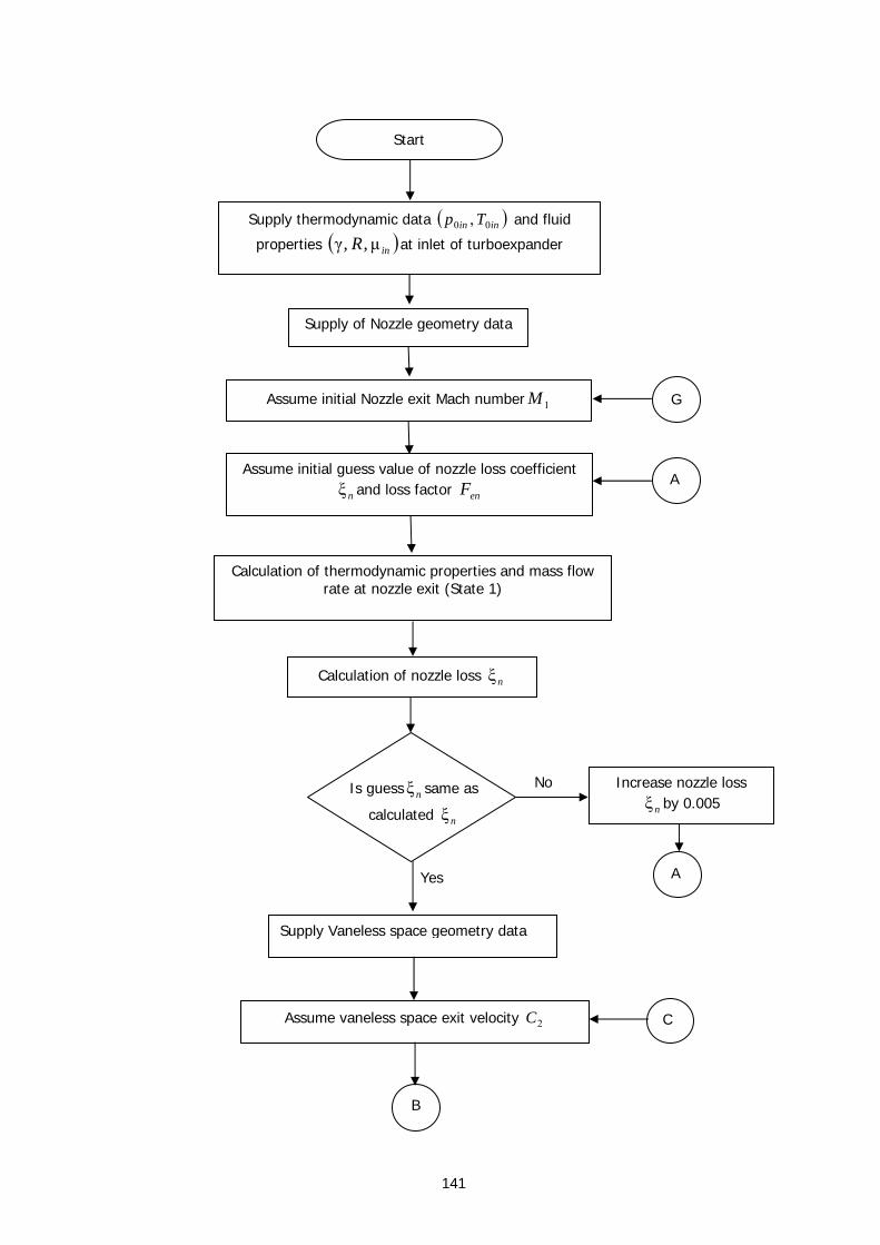
141

C

No

Yes

Is guess nξ same as

calculated nξ

B

Increase nozzle loss

nξ by 0.005

A

Assume initial guess value of nozzle loss coefficient

nξ and loss factor enF

Calculation of thermodynamic properties and mass flow rate at nozzle exit (State 1)

Calculation of nozzle loss nξ

A

Supply of Nozzle geometry data

Start

Supply thermodynamic data ( )inin Tp 00 , and fluid

properties ( )in,R, μγ at inlet of turboexpander

Assume initial Nozzle exit Mach number 1M G

Supply Vaneless space geometry data

Assume vaneless space exit velocity 2C

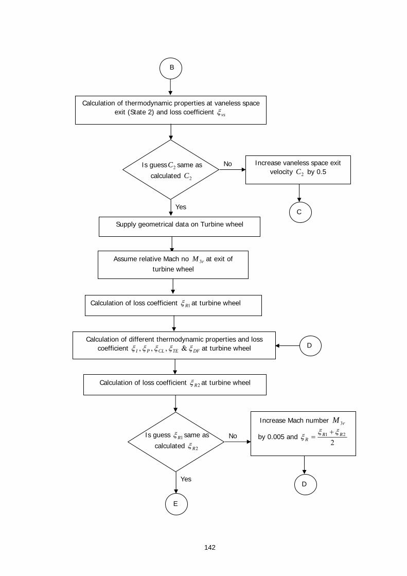
142

B

Supply geometrical data on Turbine wheel

Calculation of thermodynamic properties at vaneless space exit (State 2) and loss coefficient vsξ

Is guess 2C same as

calculated 2C

No

Yes

Increase vaneless space exit velocity 2C by 0.5

C

Calculation of loss coefficient 1Rξ at turbine wheel

Assume relative Mach no rM 3 at exit of turbine wheel

Is guess 1Rξ same as

calculated 2Rξ No

Yes

Increase Mach number rM 3

by 0.005 and 2

21 RRR

ξξξ

+=

D

D Calculation of different thermodynamic properties and loss

coefficient DFTECLPI ξξξξξ &,,, at turbine wheel

Calculation of loss coefficient 2Rξ at turbine wheel

E

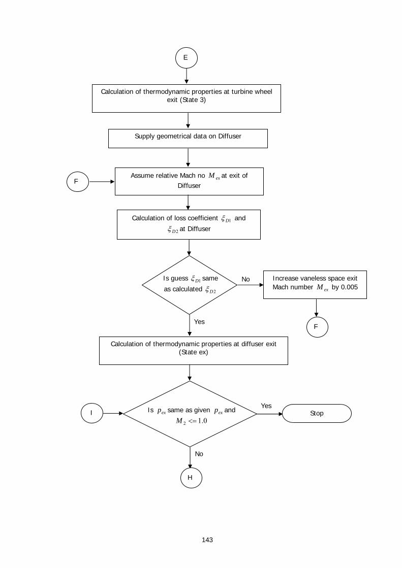
143

Calculation of thermodynamic properties at turbine wheel exit (State 3)

E

Calculation of loss coefficient 1Dξ and

2Dξ at Diffuser

Assume relative Mach no exM at exit of Diffuser

Is guess 1Dξ same

as calculated 2Dξ No

Yes

Increase vaneless space exit Mach number exM by 0.005

F

F

Calculation of thermodynamic properties at diffuser exit (State ex)

Is exp same as given exp and

0.12 <=M

No

YesStop

H

I

Supply geometrical data on Diffuser

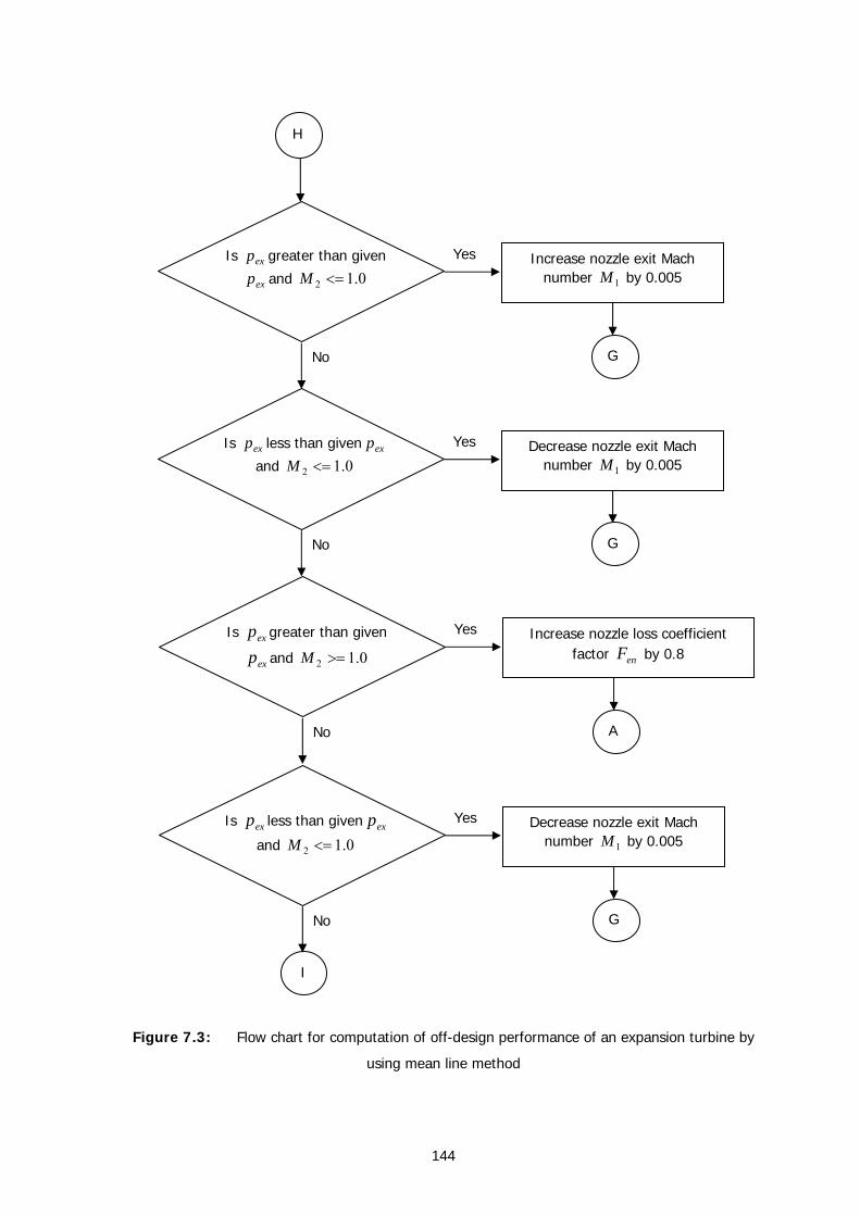
144

Figure 7.3: Flow chart for computation of off-design performance of an expansion turbine by

using mean line method

Decrease nozzle exit Mach number 1M by 0.005

G

Is exp less than given exp

and 0.12 <=M

No

Yes

Increase nozzle loss coefficient factor enF by 0.8

A

Is exp greater than given

exp and 0.12 >=M

No

Yes

I

Decrease nozzle exit Mach number 1M by 0.005

G

Is exp less than given exp

and 0.12 <=M

No

Yes

H

Increase nozzle exit Mach number 1M by 0.005

G

Is exp greater than given

exp and 0.12 <=M

No

Yes

145

7.7 Results and discussion A numerical model of the cryogenic turboexpander has been developed covering all the

constituent units of the turboexpander system to predict its performance under varying operating

conditions. The meanline analysis is carried out in this section and brings out many important

features of turbine performance. A computer program for this procedure has been written in C.

This program uses turbine geometry as input and computes the performance over a range of

rotational speed and pressure ratio.

While most major effects have been included, a few known sources of inefficiency have

been excluded because of the unavailability of appropriate loss correlations. The losses caused by

tip axial and radial clearances, trailing edge thickness and surface roughness have been carried

out to asses their influence on turbine performance. Computation has been performed over a

pressure ratio range of 1.2 to 6.5, at five different values of design speed, i.e. 50%, 75%, 100%,

125% and 150% of the design speed. The followings are some of the major observations from

the computed results.

The performance of a turbomachine can be presented in terms of some non-

dimensionless groups like pressure ratio, mass flow function, efficiency and velocity ratio.

Performance maps for the designed turbine are shown in Figures 7.4 and 7.5. The mass flow rate

increases monotonically with increase in pressure ratio but decreases with that of rotational

speed. It is almost constant after a certain pressure ratio due to chocked flow. Similarly the

efficiency increases initially with pressure ratio but decreases after a certain value of pressure

ratio. For a particular pressure ratio the efficiency depends on rotational speed. The maximum

total to static efficiency of 57.8% is attained for a pressure ratio of 2.6 at the design speed.

The loss coefficient and losses in unit of Watt at the design speed in the basic units of

turboexpander are shown in Figure 7.6 to 7.7. From these figures it can be seen that the

maximum loss occurs in the turbine wheel compared to other units and the loss in the turbine

wheel increases with pressure ratio, whereas the losses in nozzle, vaneless space and diffuser are

almost constant with pressure ratio. Figure 7.8 shows the different loss coefficients in the turbine

wheel. The passage loss is the highest in turbine wheel and increases with pressure ratio. The

trailing edge loss and incidence loss decrease initially with pressure ratio but after a certain

pressure ratio these losses remain constant. The clearance loss and disk friction loss are small

compared to other losses in the turbine wheel.

The variation of Mach number over the different units along the fluid path is shown in

Figure 7.9. The Mach number increases with pressure ratio in all the units. The Mach number at

the inlet of the turbine wheel is the highest and approaches unity at a certain pressure ratio.

The loss coefficients in the nozzle, vaneless space, turbine wheel and diffuser are shown

in Figure 7.10 to 7.13. From Figures 7.10 and 7.11 it can be seen that the loss coefficients in the

146

nozzle and vaneless space decrease with pressure ratio and rotational speed. The turbine and

diffuser loss coefficients increase with pressure ratio at low rotational speeds but almost remain

constant with pressure ratio at high rotational speeds as shown in Figures 7.12 and 7.13. From

the Figures 7.14 to 7.17, it is observed that the losses in the basic units of the turboexpander

operating with different rotational speeds increase with increase of pressure ratio. The loss at a

particular pressure is lower at higher rotational speed. As the rotational speed increases, the back

pressure generated by centrifugal forces also increases, thereby reducing the mass flow rate. At

lower flow rate, the velocity in the nozzle is lower, thus reducing the losses.

As the turbine loss is highest, different loss coefficient for different rotational speed is

shown in Figures 7.18 to 7.22. Figure 7.18 shows the incidence loss coefficient. It decreases with

increase of pressure ratio but increases with increase of high rotational speed. Figure 7.19 helps

to visualize the influence of pressure ratio on passage loss coefficient at different rotational

speeds. The passage loss is observed to be increasing with pressure ratio and decreasing with

rotational speed. At higher pressure ratios, the relative velocity in the wheel is higher, thus

increasing the passage loss. At higher rotational speeds, the back pressure in the rotor increases,

thereby decreasing mass flow rate and relative velocity. As a result, the passage loss, which

varies as the square of the relative velocity, also decreases. This particular loss mechanism has

the highest contribution to the drop in performance of a small turbine. The influence of pressure

ratio at different rotational speeds on clearance loss coefficient is shown in Figure 7.20. The

clearance loss accounts for the leakage of working gas from the pressure face of a blade to the

suction face through the clearance between the rotor and the stationary shroud. The clearance

loss coefficient decreases with pressure ratio but increases with rotational speed. The variation of

trailing edge loss coefficient with increasing pressure ratio for different rotational speeds is shown

in Figure 7.21. The trailing edge loss coefficient decreases with pressure ratio and increases with

rotational speed. The disk friction loss coefficient is very small compared to other loss coefficients

as shown in Figure 7.22. The disk friction loss coefficient decreases with increase of pressure

ratio and increases with increase of rotational speed.

The influence of pressure ratio and rotational speed on Mach number is shown for all

basic units of the turboexpander in Figures 7.23 to 7.26. At all the units, the Mach number

increases with pressure ratio but at a particular pressure ratio the Mach number is higher for low

rotational speeds.

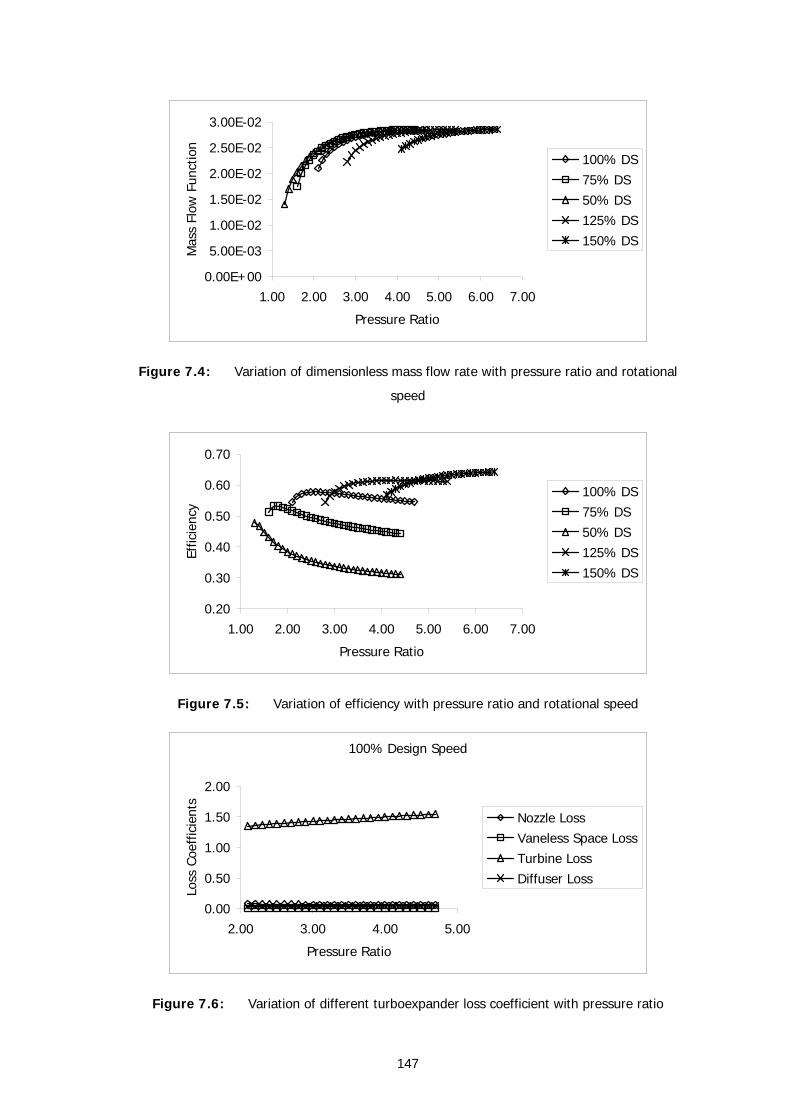
147

0.00E+00

5.00E-03

1.00E-02

1.50E-02

2.00E-02

2.50E-02

3.00E-02

1.00 2.00 3.00 4.00 5.00 6.00 7.00

Pressure Ratio

Mas

s Fl

ow F

unct

ion

100% DS75% DS50% DS125% DS150% DS

Figure 7.4: Variation of dimensionless mass flow rate with pressure ratio and rotational

speed

0.20

0.30

0.40

0.50

0.60

0.70

1.00 2.00 3.00 4.00 5.00 6.00 7.00

Pressure Ratio

Effic

ienc

y

100% DS75% DS50% DS125% DS150% DS

Figure 7.5: Variation of efficiency with pressure ratio and rotational speed

100% Design Speed

0.00

0.50

1.00

1.50

2.00

2.00 3.00 4.00 5.00

Pressure Ratio

Loss

Coe

ffic

ient

s

Nozzle LossVaneless Space LossTurbine LossDiffuser Loss

Figure 7.6: Variation of different turboexpander loss coefficient with pressure ratio

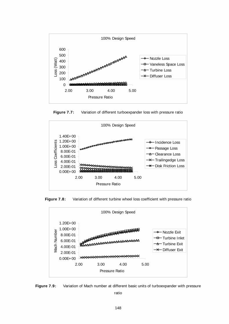
148

100% Design Speed

0100200300400500600

2.00 3.00 4.00 5.00

Pressure Ratio

Loss

(W

att) Nozzle Loss

Vaneless Space LossTurbine LossDiffuser Loss

Figure 7.7: Variation of different turboexpander loss with pressure ratio

100% Design Speed

0.00E+002.00E-014.00E-016.00E-018.00E-01

1.00E+001.20E+001.40E+00

2.00 3.00 4.00 5.00

Pressure Ratio

Loss

Coe

ffic

ient

s Incidence LossPassage LossClearance LossTrailingedge LossDisk Friction Loss

Figure 7.8: Variation of different turbine wheel loss coefficient with pressure ratio

100% Design Speed

0.00E+002.00E-014.00E-016.00E-018.00E-01

1.00E+001.20E+00

2.00 3.00 4.00 5.00

Pressure Ratio

Mac

h N

umbe

r

Nozzle ExitTurbine InletTurbine ExitDiffuser Exit

Figure 7.9: Variation of Mach number at different basic units of turboexpander with pressure

ratio

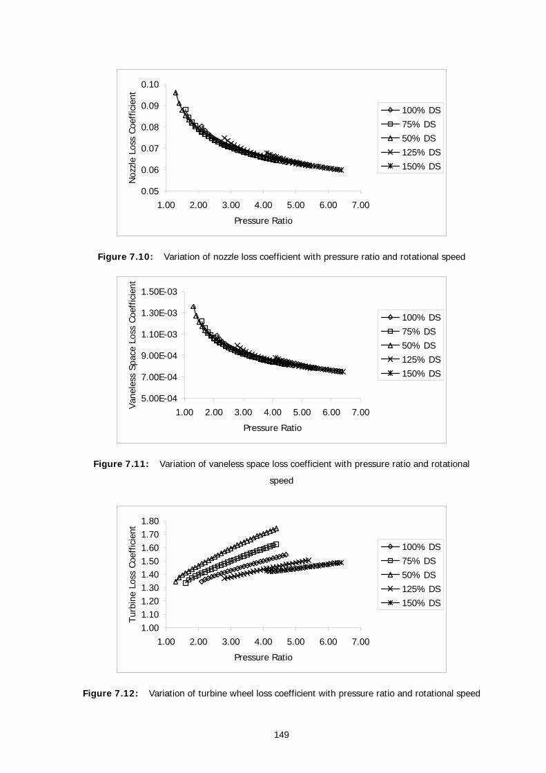
149

0.05

0.06

0.07

0.08

0.09

0.10

1.00 2.00 3.00 4.00 5.00 6.00 7.00

Pressure Ratio

Noz

zle

Loss

Coe

ffic

ient

100% DS75% DS50% DS125% DS150% DS

Figure 7.10: Variation of nozzle loss coefficient with pressure ratio and rotational speed

5.00E-04

7.00E-04

9.00E-04

1.10E-03

1.30E-03

1.50E-03

1.00 2.00 3.00 4.00 5.00 6.00 7.00

Pressure Ratio

Vane

less

Spa

ce L

oss

Coef

ficie

nt

100% DS75% DS50% DS125% DS150% DS

Figure 7.11: Variation of vaneless space loss coefficient with pressure ratio and rotational

speed

1.001.101.201.301.401.501.601.701.80

1.00 2.00 3.00 4.00 5.00 6.00 7.00

Pressure Ratio

Turb

ine

Loss

Coe

ffic

ient

100% DS75% DS50% DS125% DS150% DS

Figure 7.12: Variation of turbine wheel loss coefficient with pressure ratio and rotational speed

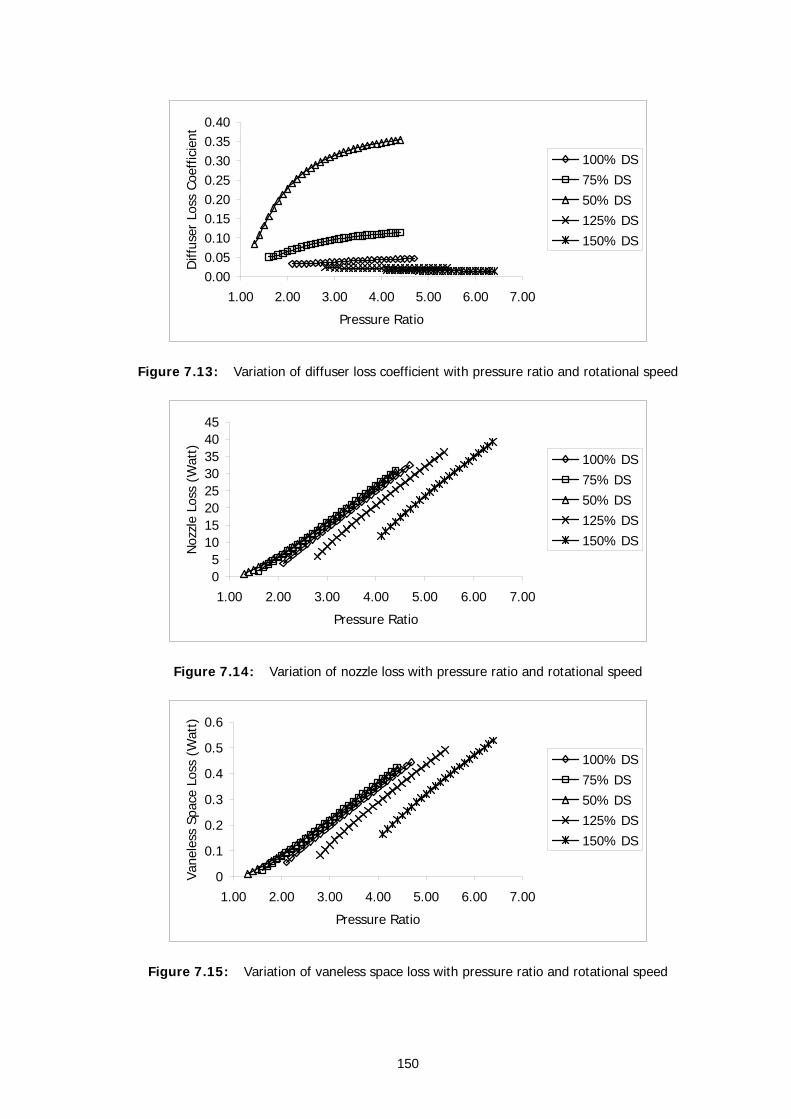
150

0.000.050.100.150.200.250.300.350.40

1.00 2.00 3.00 4.00 5.00 6.00 7.00

Pressure Ratio

Diff

user

Los

s Co

effic

ient

100% DS75% DS50% DS125% DS150% DS

Figure 7.13: Variation of diffuser loss coefficient with pressure ratio and rotational speed

05

1015202530354045

1.00 2.00 3.00 4.00 5.00 6.00 7.00

Pressure Ratio

Noz

zle

Loss

(W

att)

100% DS75% DS50% DS125% DS150% DS

Figure 7.14: Variation of nozzle loss with pressure ratio and rotational speed

0

0.1

0.2

0.3

0.4

0.5

0.6

1.00 2.00 3.00 4.00 5.00 6.00 7.00

Pressure Ratio

Vane

less

Spa

ce L

oss

(Wat

t)

100% DS75% DS50% DS125% DS150% DS

Figure 7.15: Variation of vaneless space loss with pressure ratio and rotational speed

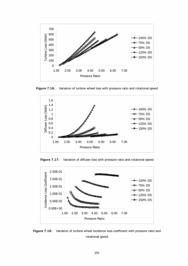
151

0

100

200

300

400

500

600

700

1.00 2.00 3.00 4.00 5.00 6.00 7.00

Pressure Ratio

Turb

ine

Loss

(W

att)

100% DS75% DS50% DS125% DS150% DS

Figure 7.16: Variation of turbine wheel loss with pressure ratio and rotational speed

00.20.40.60.8

11.21.41.6

1.00 2.00 3.00 4.00 5.00 6.00 7.00

Pressure Ratio

Diff

user

Los

s (W

att)

100% DS75% DS50% DS125% DS150% DS

Figure 7.17: Variation of diffuser loss with pressure ratio and rotational speed

0.00E+00

5.00E-02

1.00E-01

1.50E-01

2.00E-01

2.50E-01

1.00 2.00 3.00 4.00 5.00 6.00 7.00

Pressure Ratio

Inci

denc

e Lo

ss C

oeff

icie

nt

100% DS75% DS50% DS125% DS150% DS

Figure 7.18: Variation of turbine wheel incidence loss coefficient with pressure ratio and

rotational speed

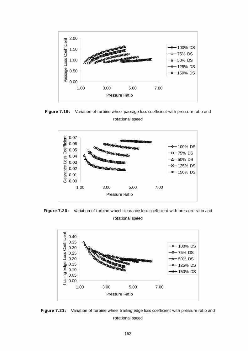
152

0.00

0.50

1.00

1.50

2.00

1.00 3.00 5.00 7.00

Pressure Ratio

Pass

age

Loss

Coe

ffic

ient

100% DS75% DS50% DS125% DS150% DS

Figure 7.19: Variation of turbine wheel passage loss coefficient with pressure ratio and

rotational speed

0.000.010.020.030.040.050.060.07

1.00 3.00 5.00 7.00

Pressure Ratio

Clea

ranc

e Lo

ss C

oeff

icie

nt

100% DS75% DS50% DS125% DS150% DS

Figure 7.20: Variation of turbine wheel clearance loss coefficient with pressure ratio and

rotational speed

0.000.050.100.150.200.250.300.350.40

1.00 3.00 5.00 7.00

Pressure Ratio

Trai

ling

Edge

Los

s Co

effic

ient

100% DS75% DS50% DS125% DS150% DS

Figure 7.21: Variation of turbine wheel trailing edge loss coefficient with pressure ratio and

rotational speed

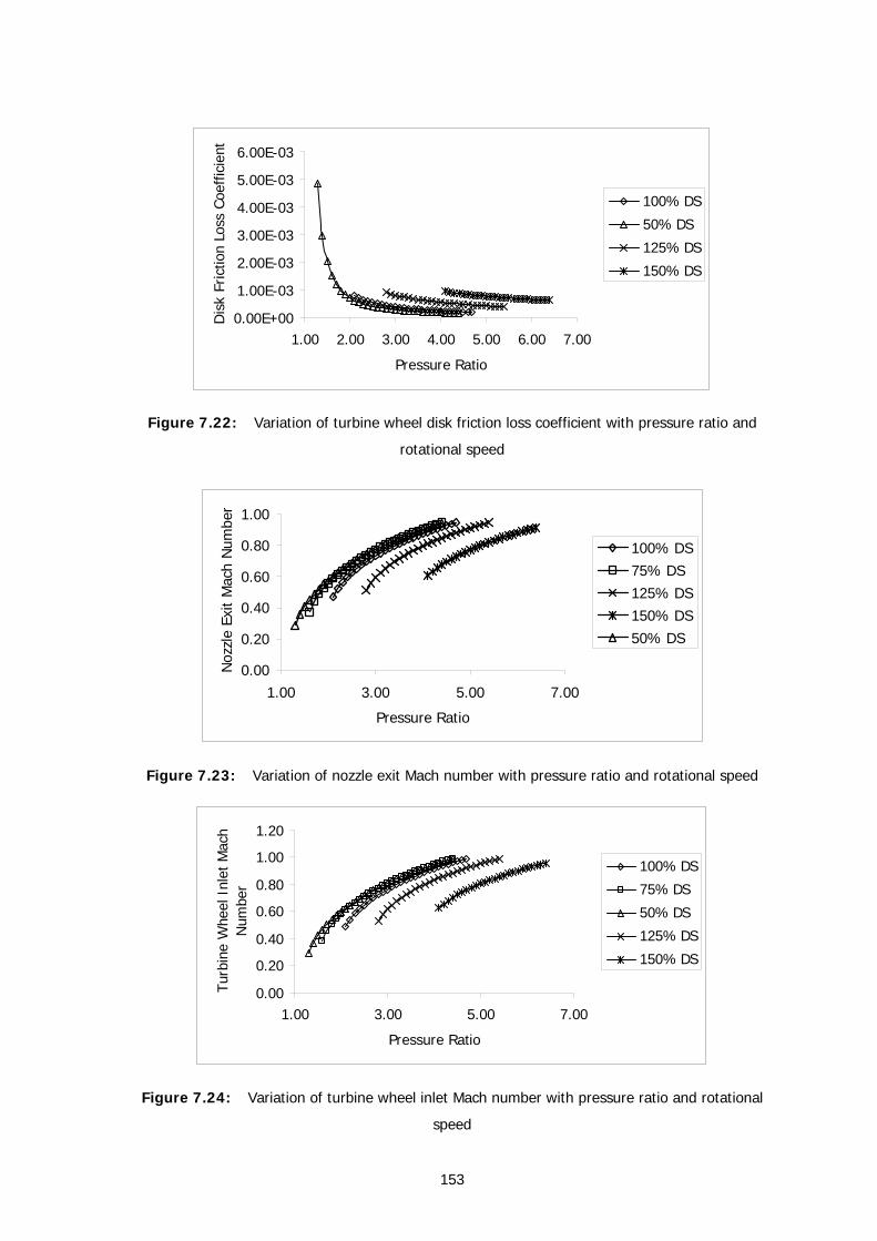
153

0.00E+00

1.00E-03

2.00E-03

3.00E-03

4.00E-03

5.00E-03

6.00E-03

1.00 2.00 3.00 4.00 5.00 6.00 7.00

Pressure Ratio

Dis

k Fr

ictio

n Lo

ss C

oeffi

cien

t100% DS

50% DS

125% DS

150% DS

Figure 7.22: Variation of turbine wheel disk friction loss coefficient with pressure ratio and

rotational speed

0.00

0.20

0.40

0.60

0.80

1.00

1.00 3.00 5.00 7.00

Pressure Ratio

Noz

zle

Exit

Mac

h N

umbe

r

100% DS75% DS125% DS150% DS50% DS

Figure 7.23: Variation of nozzle exit Mach number with pressure ratio and rotational speed

0.00

0.20

0.40

0.60

0.80

1.00

1.20

1.00 3.00 5.00 7.00

Pressure Ratio

Turb

ine

Whe

el I

nlet

Mac

h N

umbe

r

100% DS

75% DS

50% DS

125% DS

150% DS

Figure 7.24: Variation of turbine wheel inlet Mach number with pressure ratio and rotational

speed

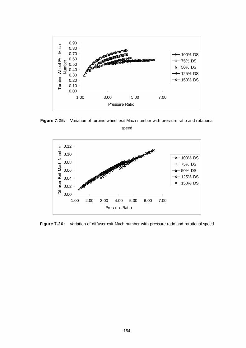
154

0.000.100.200.300.400.500.600.700.800.90

1.00 3.00 5.00 7.00

Pressure Ratio

Turb

ine

Whe

el E

xit

Mac

h N

umbe

r

100% DS75% DS50% DS125% DS150% DS

Figure 7.25: Variation of turbine wheel exit Mach number with pressure ratio and rotational

speed

0.00

0.02

0.04

0.06

0.08

0.10

0.12

1.00 2.00 3.00 4.00 5.00 6.00 7.00

Pressure Ratio

Diff

user

Exi

t M

ach

Num

ber

100% DS75% DS50% DS125% DS150% DS

Figure 7.26: Variation of diffuser exit Mach number with pressure ratio and rotational speed

Chapter VIII

EPILOGUE

Small turboexpanders have found extensive application particularly in cryogenic

refrigeration and liquefaction systems, small liquid oxygen and nitrogen generators, helium

liquefiers and emergency power packs. While the basic technological principles are well

established, finer aspects of technology still remain proprietary information in the hands of a

handful of international companies. The work reported in this thesis is an attempt at designing

and developing an indigenous turboexpander system through numerical analysis and

experimentation. A major aspect of the investigation is the study of different bearings types and

the performance under varying operating conditions. Two different types of thrust bearings and

one class of journal bearings have been used in the experimental study. While tilting pad journal

bearings have performed very well, there are still questions on the right choice for the thrust

bearings. In order to understand the performance of the turboexpander under off design

conditions, a complete performance map of the specified turbine system has been generated.

8.1 Concluding remarks

This work is a modest attempt at studying a cryogenic turboexpander through

experimental and theoretical analyses. Summarising, the following may be seen as the significant

contributions of the present investigation.

i). The thesis presents an updated literature review on almost all aspects of cryogenic

turboexpander, and may serve as a ready reference for future work.

ii). A comprehensive methodology for the design of a turboexpander has been presented. A

prototype expander has been designed, constructed and experimented using this recipe.

iii). The design procedure covers not only the turbine wheel, but also the associated

components such as compressor, shaft, bearings, seals and structural members. While

some of the dimensions have been computed, others have been selected based on

experimented evidence. The component layout has been worked out keeping the critical

clearances and tolerances in view.

156

iv). A numerical model has been developed for parametric analysis and its effect on the

turbine blade profile.

v). A parametric analysis of the blade design process reveals that an optimum value exists

for the free parameters that eliminates the possibility of a dumb-bell shaped blade and

leads to an optimised path length. Optimum values of hk (= 5.0) and ek (=0.75) lead to

the highest machine efficiency with exit radial component 3δ as 9°.

vi). Two experimental test set ups have been constructed in the Cryogenics Laboratory of

NIT Rourkela to study the behaviour of the turbine based on aerostatic and aerodynamic

thrust bearings.

vii). The prototype expander with aerostatic thrust bearings has been tested at 100,000 r/min

giving a temperature drop of 16ºC, whereas the aerodynamic grooved thrust bearings

sustained a rotational speed of 200,000 r/min while giving a temperature drop of 30ºC.

viii). It has been observed that the spiral grooved thrust bearings have performed consistently

well, but need to be protected against rubbing during start ups and shutdown.

ix). A formal procedure has been developed for predicting the performance of the turbine

under varying operating conditions, and for studying the effects of geometrical features

such as clearances, surface roughness on turbine etc.

x). The maximum total to static efficiency of 57.8% is attained at a pressure ratio of 2.6 for

the design speed.

xi). The mass flow rate has been observed to increase with increase with pressure ratio and

to decrease with rotational speed. Beyond a specified pressure ratio, it remains almost

constant with increase of pressure ratio.

xii). Turbine total to static efficiency increases initially with pressure ratio but decreases

beyond a certain pressure ratio.

xiii). While studying losses in a turbine, it has been observed that the maximum loss occurs in

the turbine wheel compared to other units of the turboexpander and that this loss

increases with increase in pressure ratio.

8.2 Scope for future work

Development of a sophisticated engineering product like the cryogenic expansion turbine

is a continuous process. A lot of work is yet to be done on the system reliability and

standardisation before the turboexpander can be used safely in refrigerators and liquefiers.

However it can be presumed that the valuable experience gained with the design and fabrication

of the turboexpander and associated components have resulted in the generation of a knowledge

base that will enable us to design more sophisticated systems in the days to come.

157

Some further works on the topic, which may be taken up in a larger environment are the

following:

i). Design and testing of turbines with alternative bearings such as foil bearings, and study

of their stability under continuous operation.

ii). More robust numerical models for prediction of off-design characteristics of the turbine,

incorporating loss coefficients obtained from CFD and/or experiments at cryogenic

temperature.

iii). Flow analysis inside the turboexpander by using CFD.

iv). Aerostatic thrust bearings still need significant development effort.

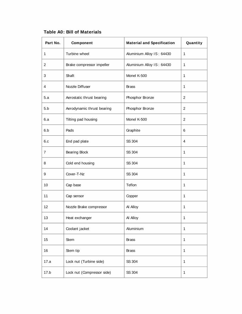
Table A0: Bill of Materials

Part No. Component Material and Specification Quantity

1 Turbine wheel Aluminium Alloy IS : 64430 1

2 Brake compressor impeller Aluminium Alloy IS : 64430 1

3 Shaft Monel K-500 1

4 Nozzle Diffuser Brass 1

5.a Aerostatic thrust bearing Phosphor Bronze 2

5.b Aerodynamic thrust bearing Phosphor Bronze 2

6.a Tilting pad housing Monel K-500 2

6.b Pads Graphite 6

6.c End pad plate SS 304 4

7 Bearing Block SS 304 1

8 Cold end housing SS 304 1

9 Cover-T-Nz SS 304 1

10 Cap base Teflon 1

11 Cap sensor Copper 1

12 Nozzle Brake compressor Al Alloy 1

13 Heat exchanger Al Alloy 1

14 Coolant jacket Aluminium 1

15 Stem Brass 1

16 Stem tip Brass 1

17.a Lock nut (Turbine side) SS 304 1

17.b Lock nut (Compressor side) SS 304 1

18.a Thermal Insulator 1 Nylon-6 1

18.b Thermal Insulator 2 Nylon-6 1

18.c Thermal Insulator 3 Teflon 1

19 Water nozzle SS 304 2

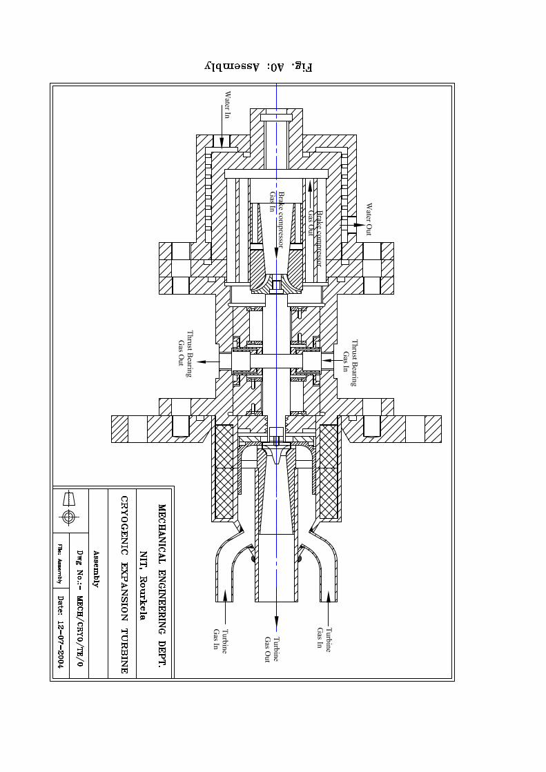
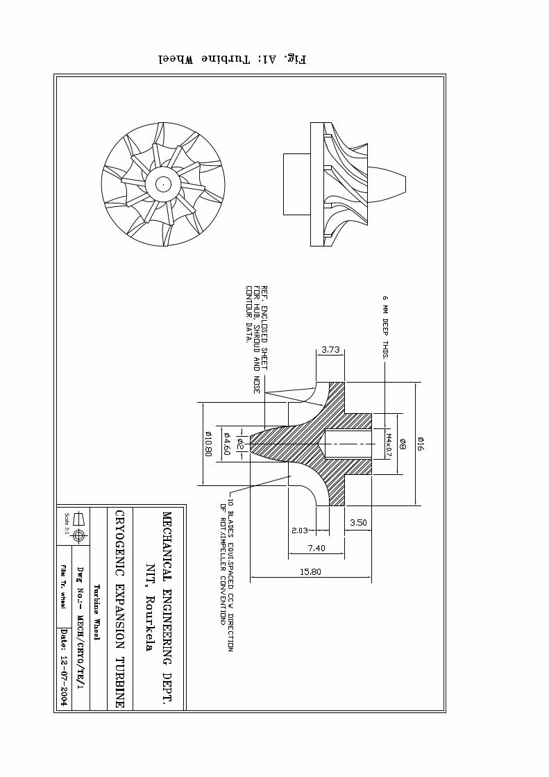
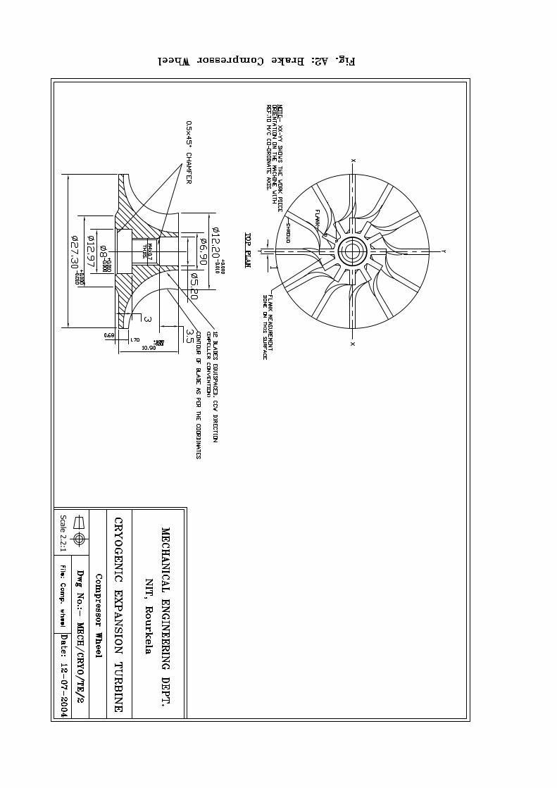
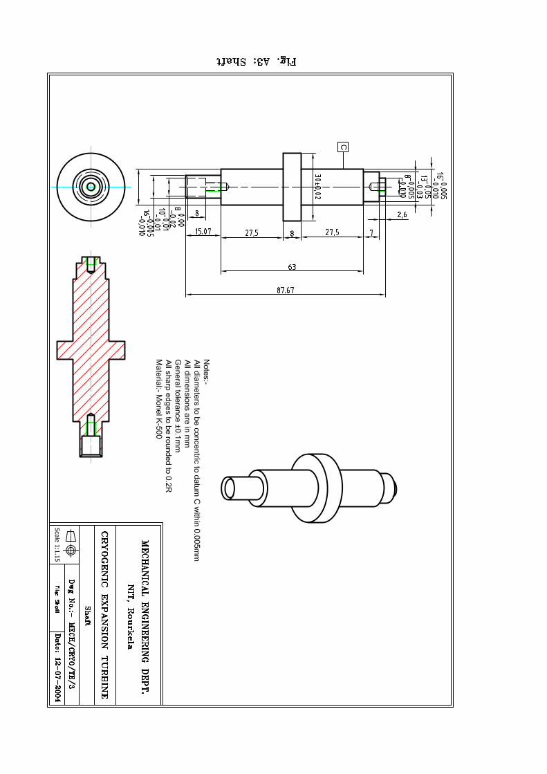
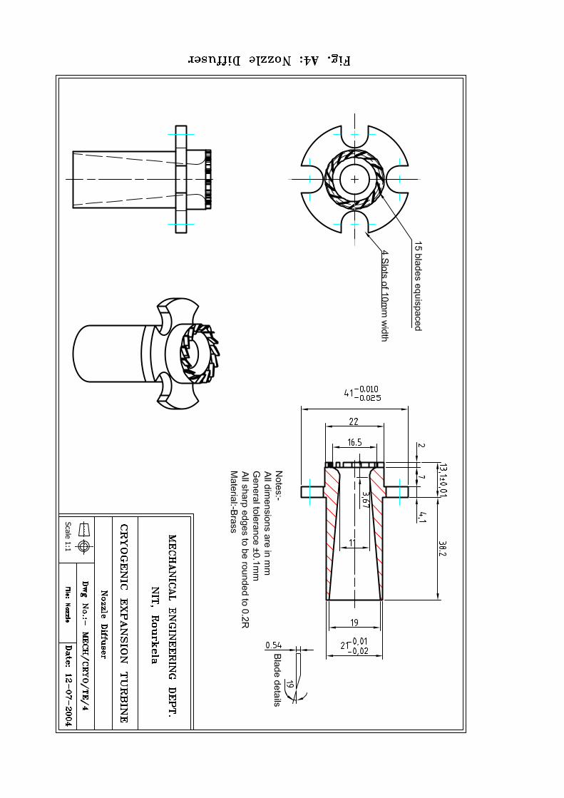
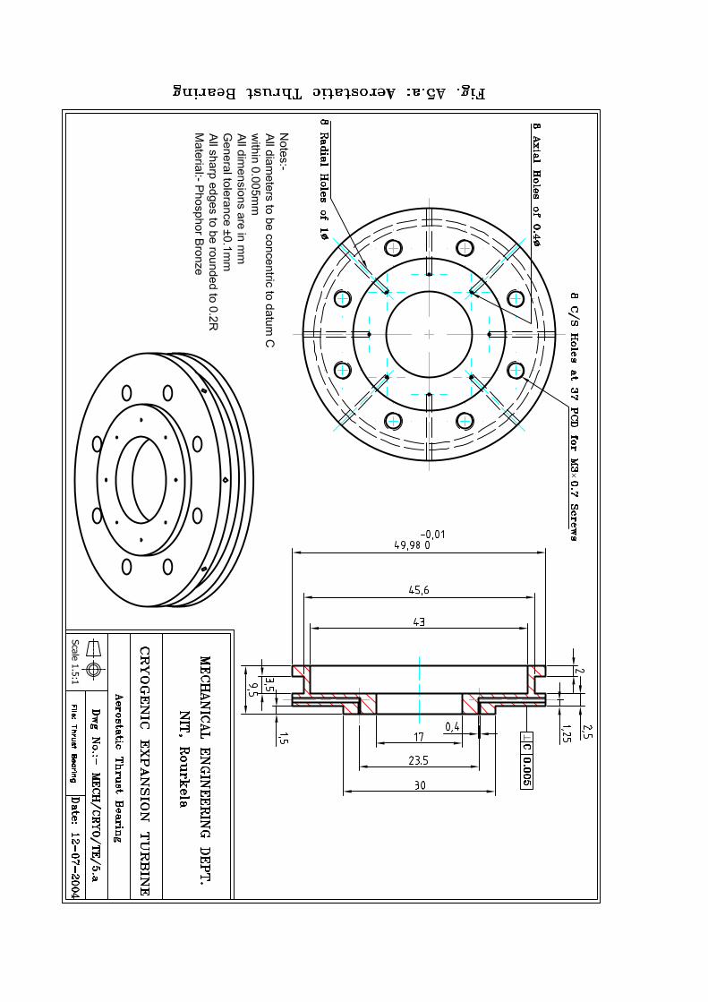
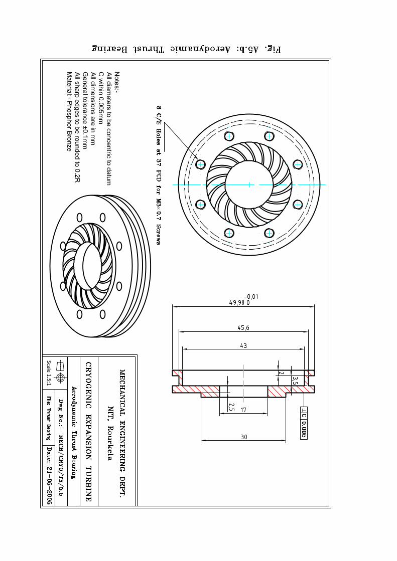
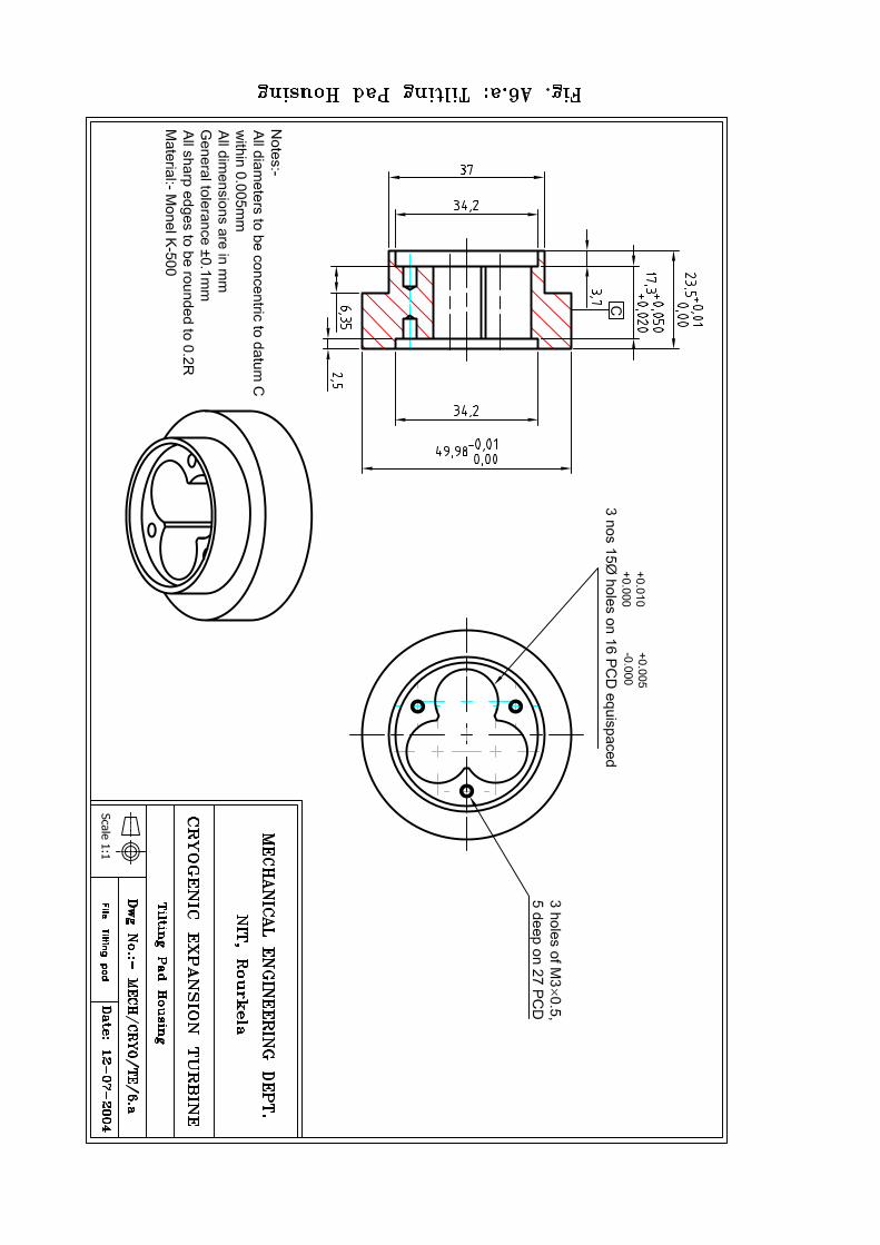
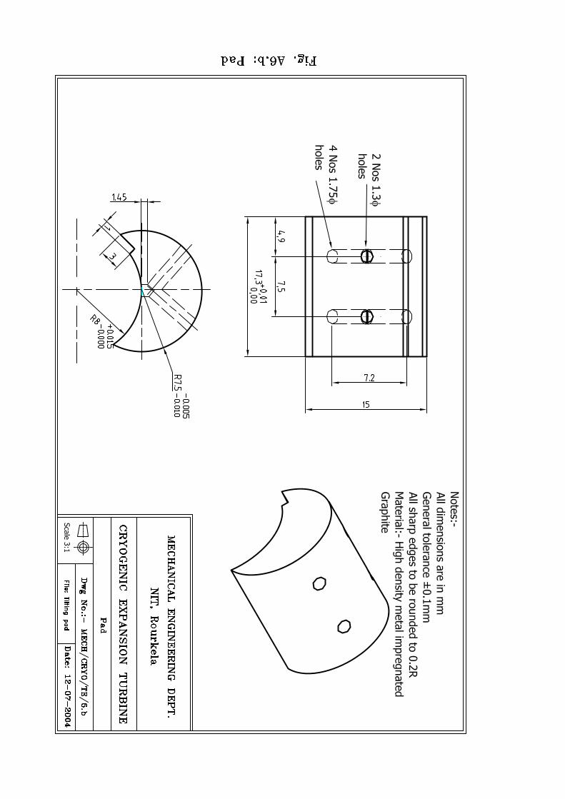
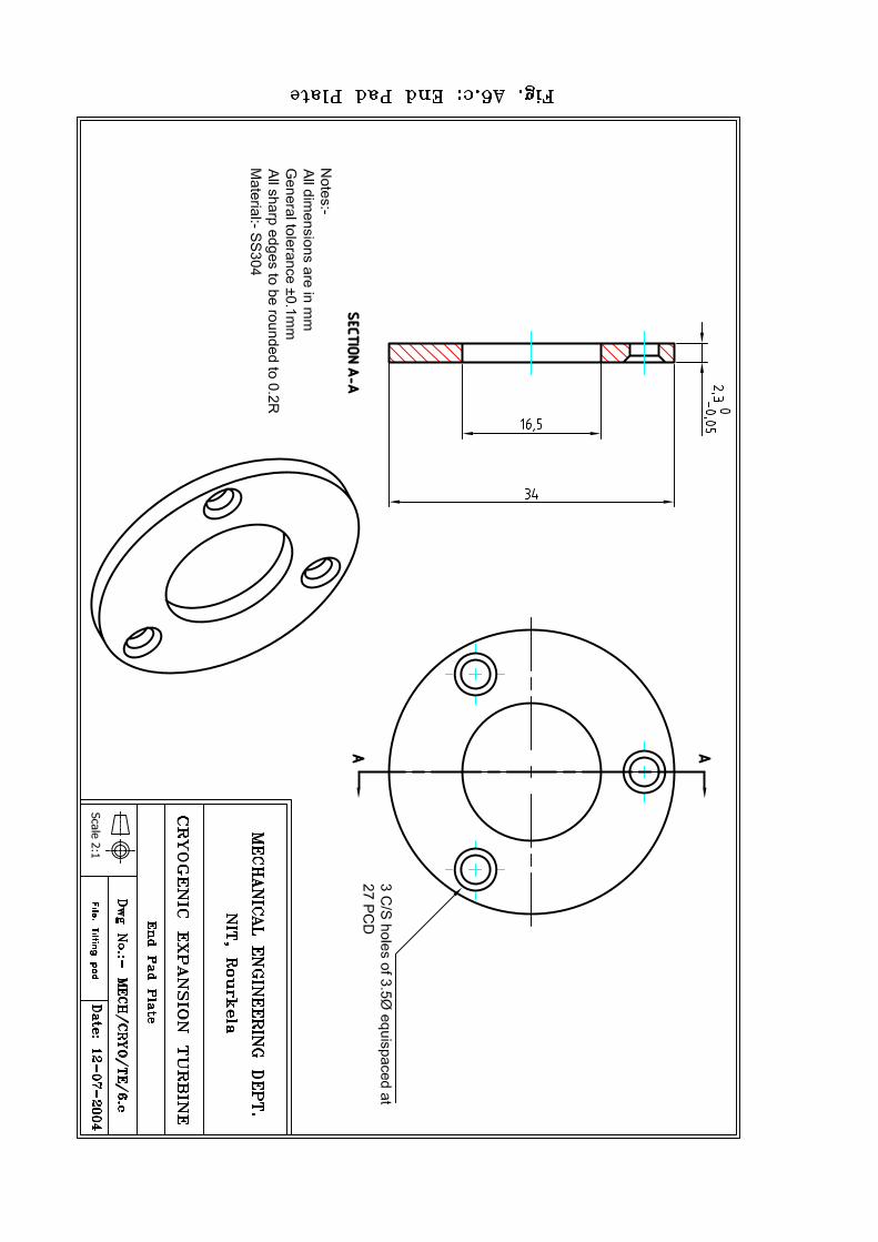
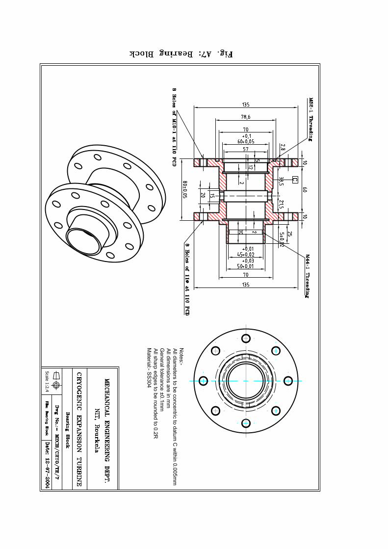
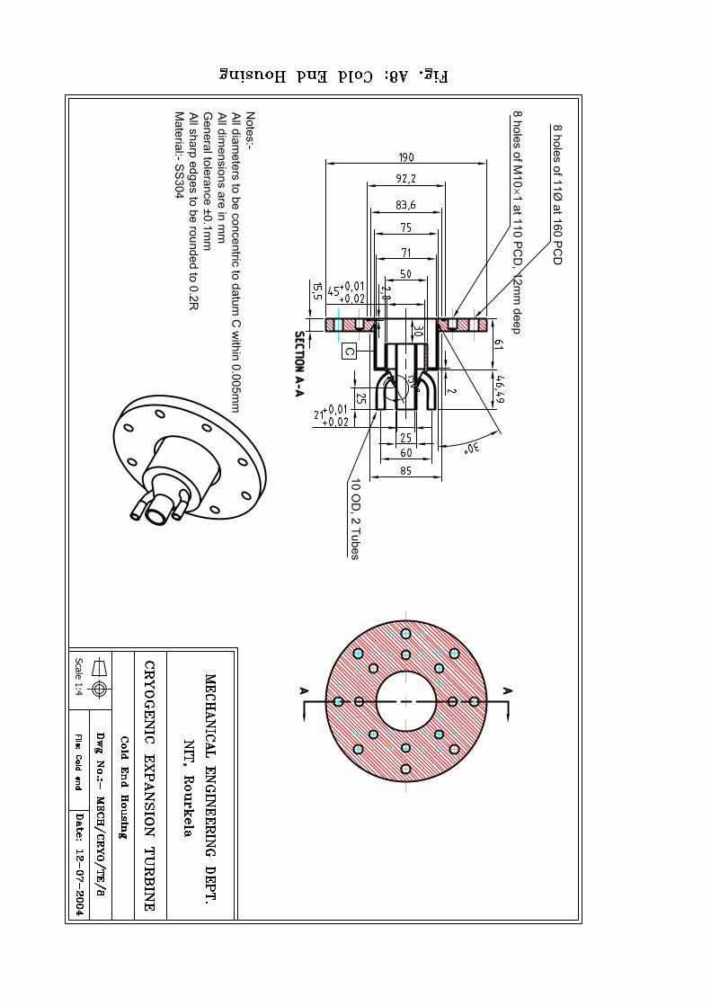
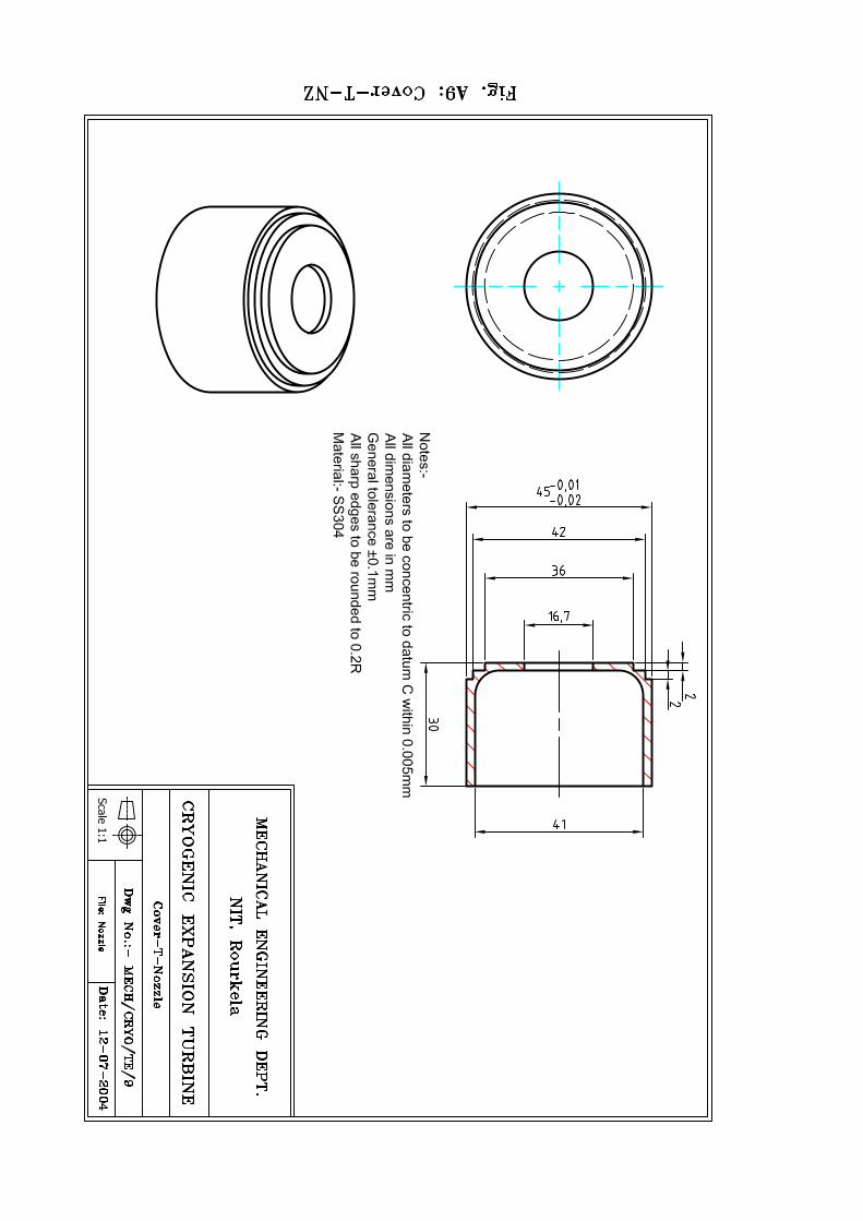
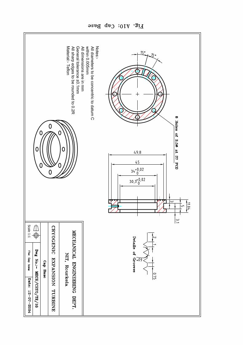
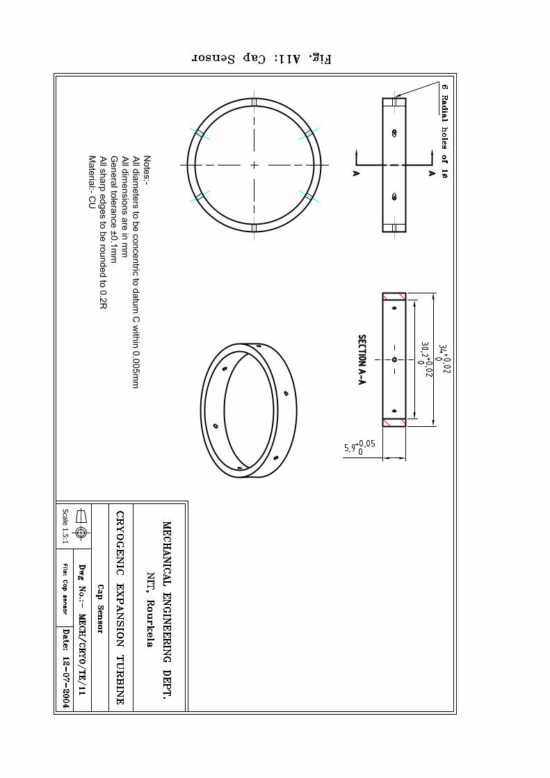
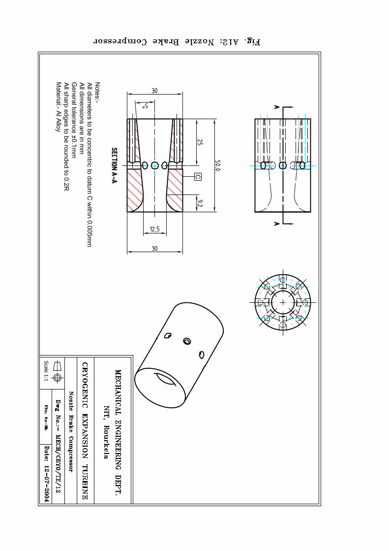
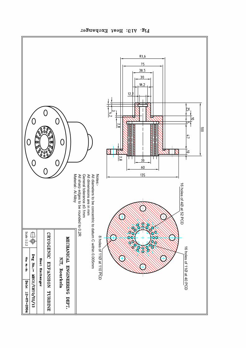
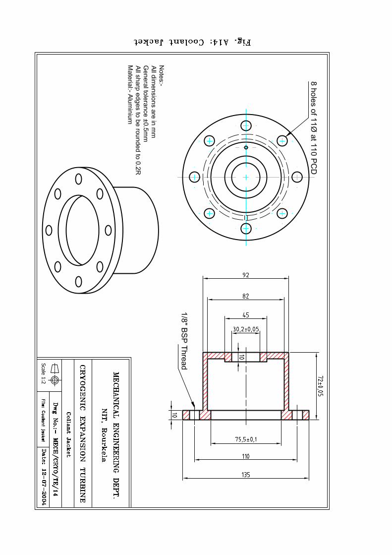
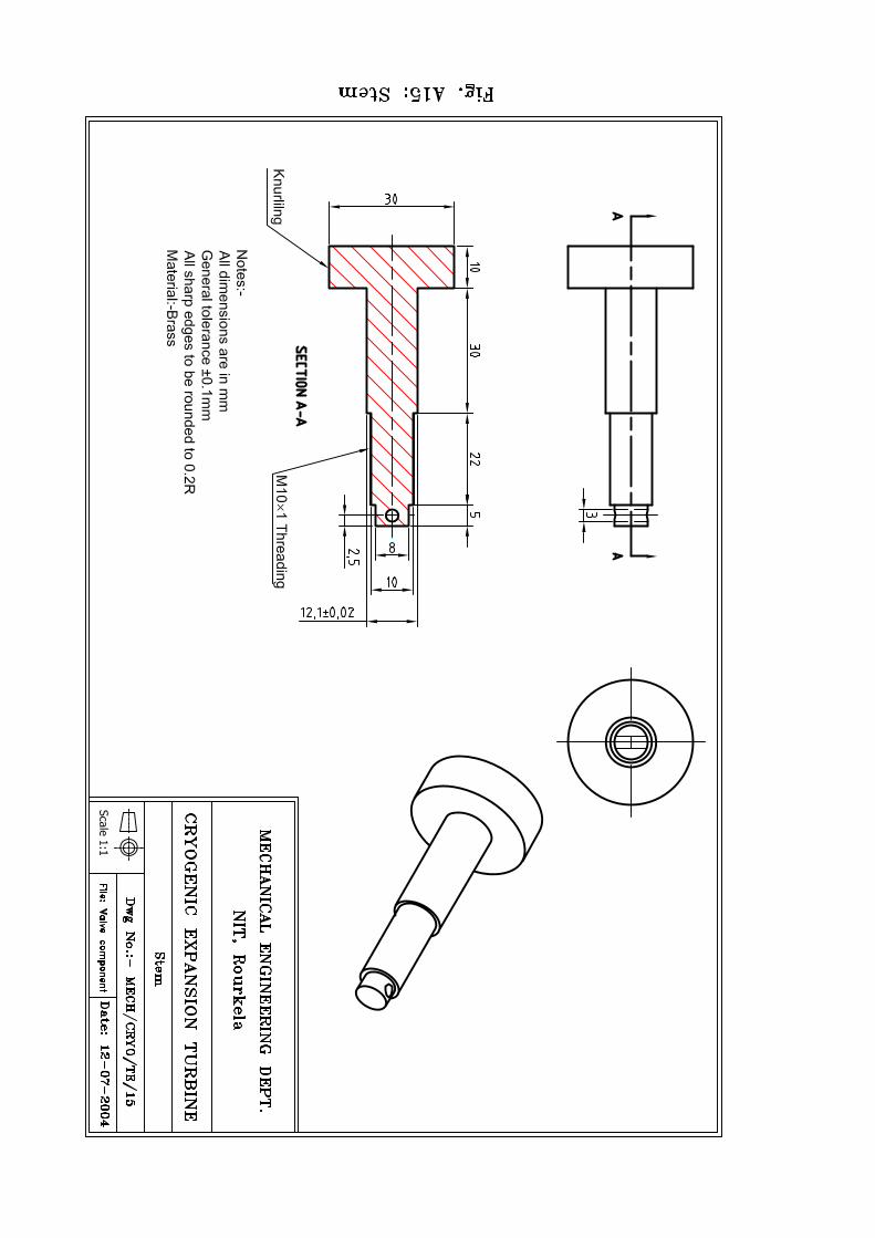
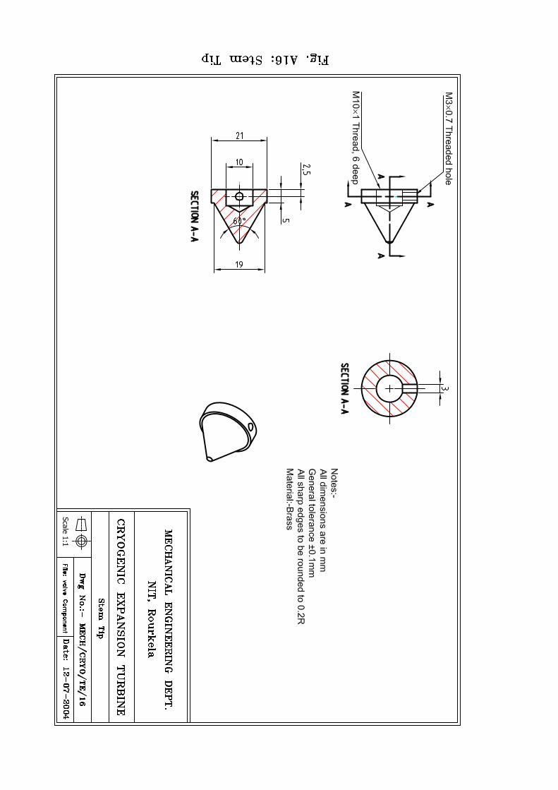
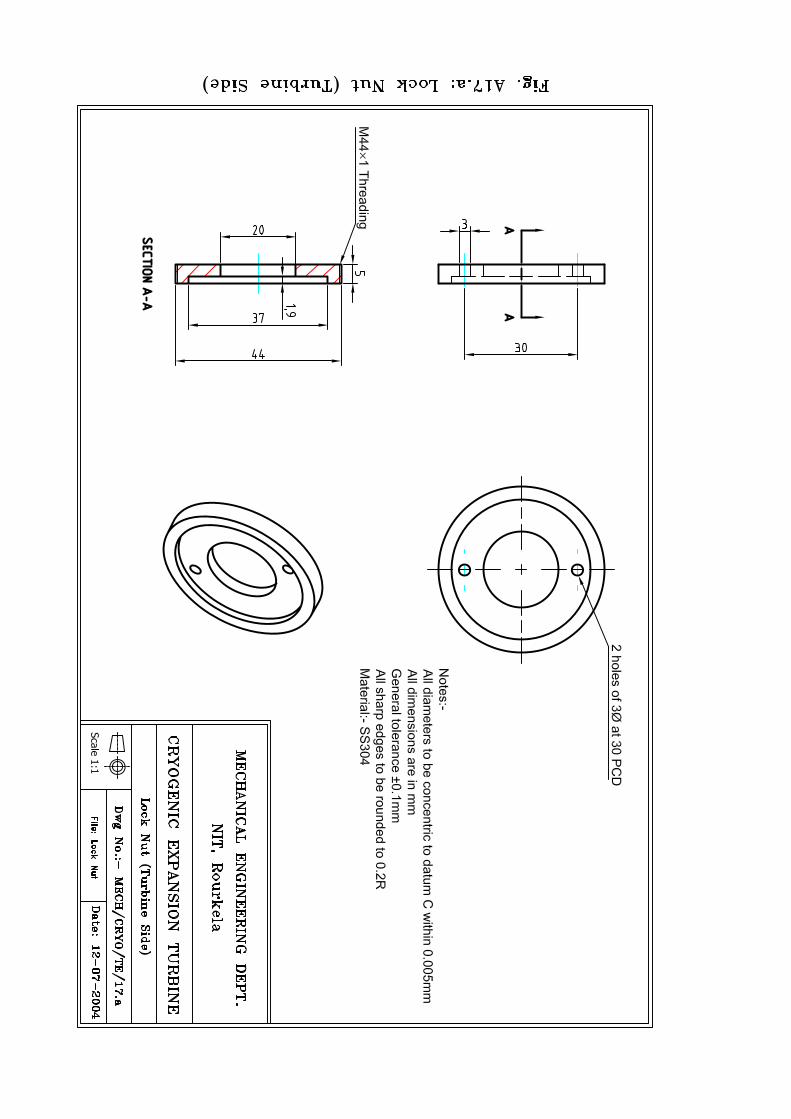
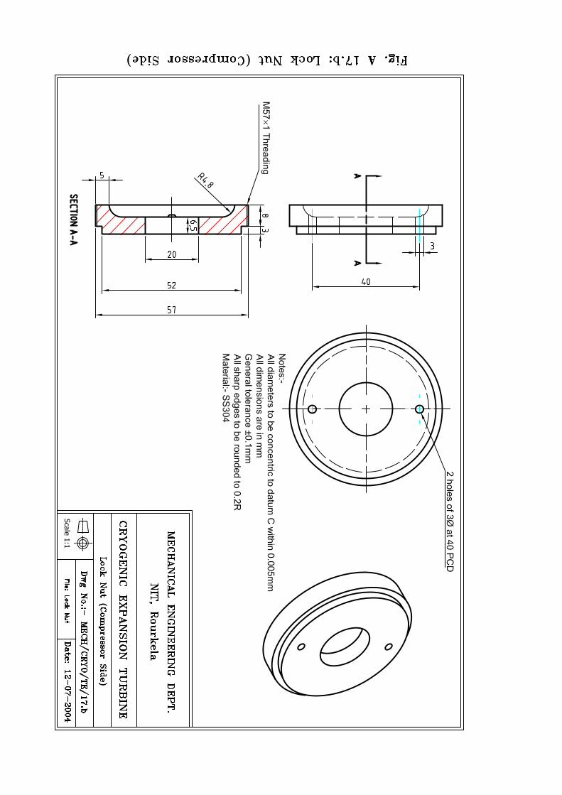
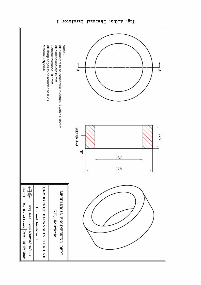
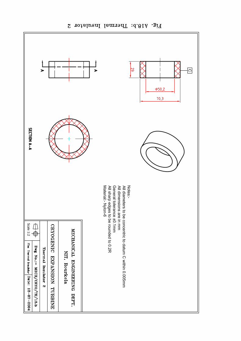
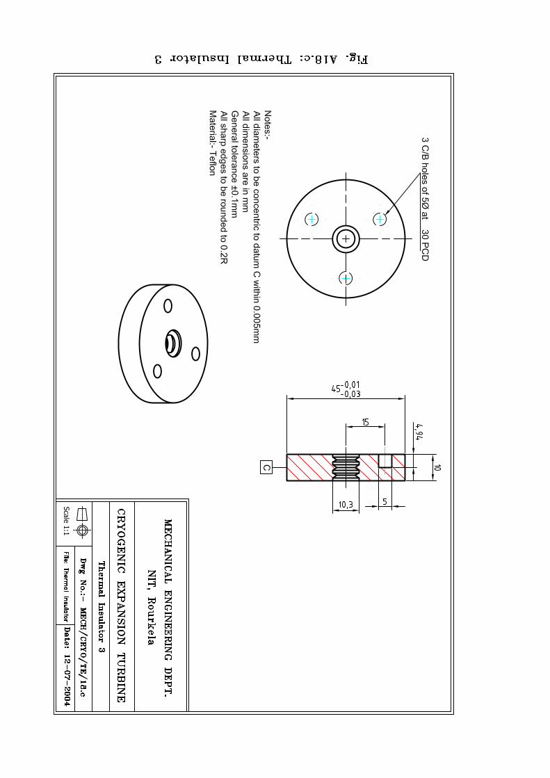
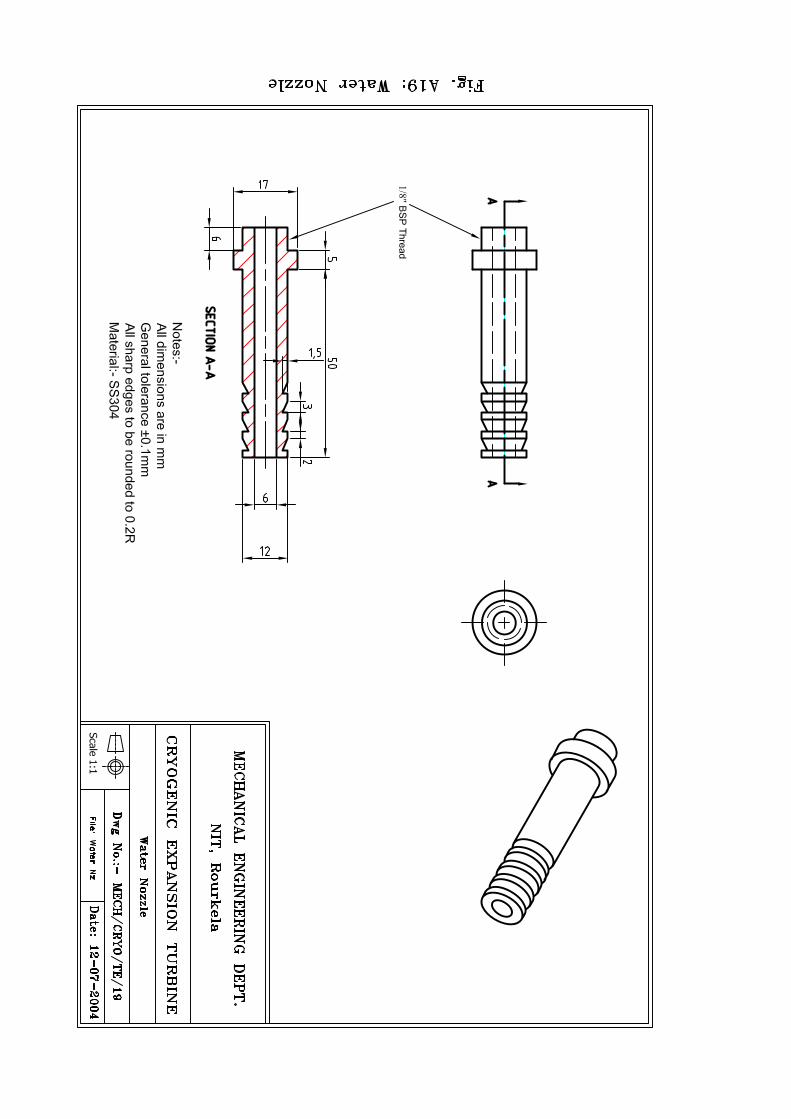
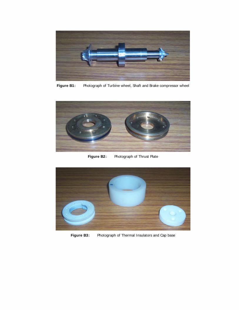
Figure B1: Photograph of Turbine wheel, Shaft and Brake compressor wheel

Figure B2: Photograph of Thrust Plate

Figure B3: Photograph of Thermal Insulators and Cap base

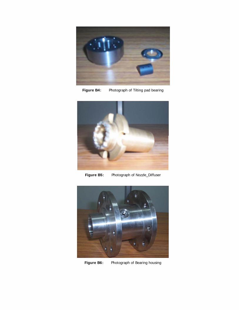
Figure B4: Photograph of Tilting pad bearing

Figure B5: Photograph of Nozzle_Diffuser

Figure B6: Photograph of Bearing housing

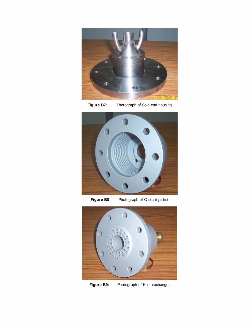
Figure B7: Photograph of Cold end housing

Figure B8: Photograph of Coolant jacket

Figure B9: Photograph of Heat exchanger

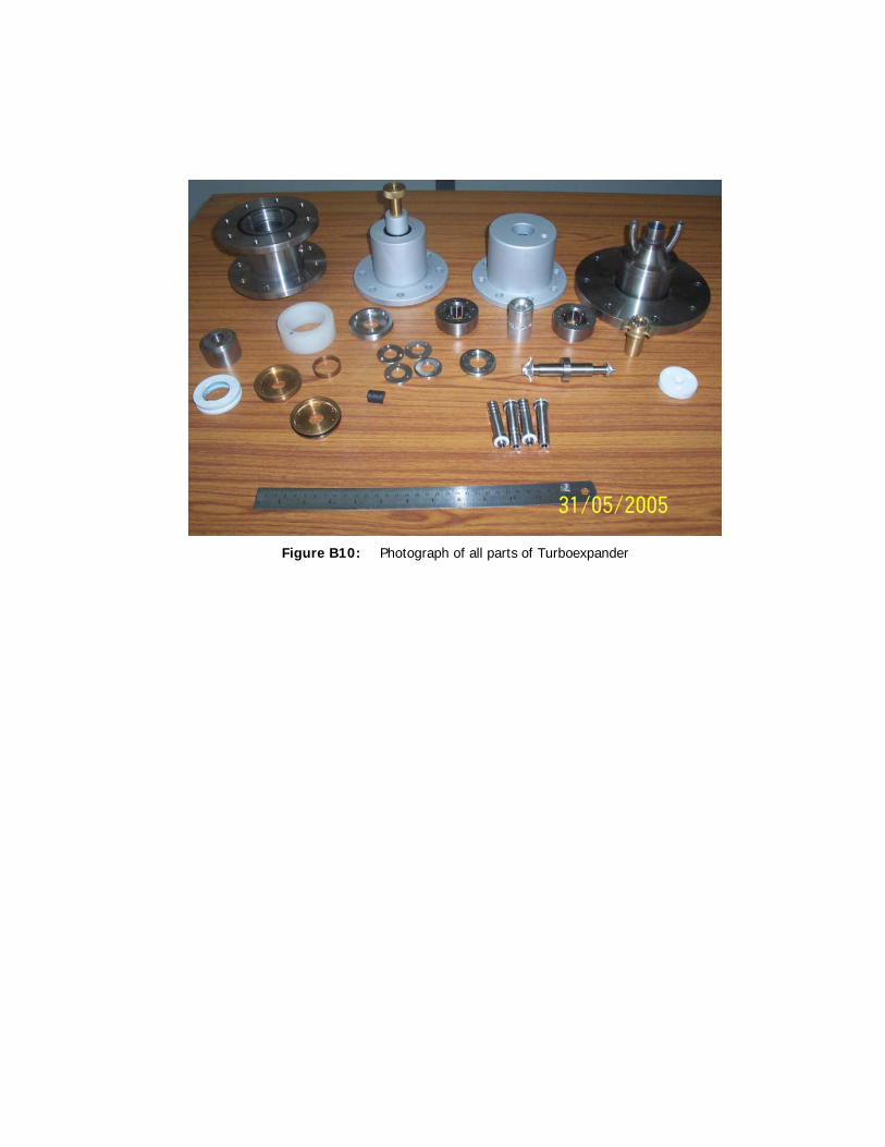
Figure B10: Photograph of all parts of Turboexpander

References 1. Barron, R. F. Cryogenic Systems Oxford University Press(1985), 131-136

2. Blackford, J. E., Halford P. and Tantam, D. H. Expander and pumps in G G Haselden (Ed) Cryogenic Fundamentals Academic Press London (1971), 403-449

3. Flynn, T.M. Cryogenic Engineering, Marcel-Dekkar Inc. (1996)

4. Timmerhaus, K. D. and Flynn T. M. Cryogenic Process Engineering Plenum Press (1989), 257-266

5. Davydov, A. B., Kobulashvili, A. Sh. and Sherstyuk, A. N. The Design and Construction of Turboexpanders [Russian] Mashinostroenie, Moscow (1987)

6. Heinz P. Bloch. and Claire Soares Turboexpander and Process applications, Gulf Professional Publishing (2001)

7. Rama S. R. Gorla and Aijaz A. Khan Turbomachinery Design and Theory, CRC Press (2003)

8. Balje, O. E. Turbomachines John Wiley and Sons (1981)

9. Dixon, S. L. Fluid Mechanics and Thermodynamics of Turbomachinery (3rd ed) Pergamon Press (1978)

10. Laxminarayana, B. Fluid Dynamics and Heat Transfer in Turbomachinary John Wiley (1996)

11. Yahya, S.M. Turbines, Compressors and Fans, Tata McGraw-Hill Publishing Co. Ltd., New Delhi (1983)

12. Glassman, A. J. (ed) Turbine Design and Application NASA SP-290 (1973)

13. Whitfield, A. and Baines, N. C. Design of Radial Turbomachines Longman Scientific & Technical (1990)

14. Moustapha, H., Zelesky, M. F., Baines, N. C. and Japikse, D. Axial and Radial turbines, Concepts ETI, Inc. (2003)

15. Sixsmith, H. Miniature cryogenic expansion turbines - a review Advances in Cryogenic Engineering (1984), V29, 511-523

16. Collins, S.C. and Cannaday, R.L. Expansion Machines for Low Temperature Processes Oxford University Press (1958)

17. Swearingen, J. S. Turbo-expanders Trans AIChE (1947), 43 (2), 85-90

18. Swearingen, J. S. Engineers' guide to turboexpanders RotoFlow Corp, USA, (1970), Gulf Publishing Company

19. Clarke, M. E. A decade of involvement with small gas lubricated turbine & Advances in Cryogenic Engineering (1974), V19, 200-208

20. Beasley, S. A. and Halford, P. Development of a High Purity Nitrogen Plant using Expansion Turbine with Gas Bearing Advances in Cryogenic Engineering (1965), V10B, 27-39

159

21. Voth, R. O., Norton, M. T. and Wilson, W. A. A cold modulator refrigerator incorporating a high speed turbine expander Advances in Cryogenic Engineering (1966), V11, 127-138

22. Colyer, D. B. Miniature cryogenic refrigerator alternators Advances in Cryogenic Engineering (1968), V13, 405-415

23. Colyer, D. B. and Gessner, R. L. Miniature cryogenic refrigerator Turbomachinary Advances in Cryogenic Engineering (1968), V13, 484-493

24. Sixsmith, H. Miniature expansion turbines, C A Bailey (Ed), Advanced Cryogenics Plenum Press (1971), 225-243

25. Schmid, C. Gas bearing turboexpanders for cryogenic plant 6th International Gas Bearing Symposium University of Southampton England (March 1974) Paper 131 B1: 1-8

26. Reuter K. and Keenan B. A. Cryogenic turboexpanders with magnetic bearings AICHE Symposium Series, Cryogenic Processes and Machinery 89 (294), 35-45

27. Izumi, H., Harada, S. and Matsubara, K. Development of small size Claude cycle helium refrigerator with micro turbo-expander Advances in Cryogenic Engineering (1986), V31, 811-818

28. Kun, L. C. and Hanson, T. C. High efficiency turboexpander in a N2 liquefier AIChE Spring meeting, Houston, Texas (1985)

29. Kun, L .C. and Sentz, R. N. High efficiency expansion turbines in air separation and liquefaction plants International Conference on Production and Purification of Coal Gas & Separation of Air, Beijing, China (1985), 1-21

30. Kun, L. C. Expansion turbines and refrigeration for gas separation and liquefaction Advances in Cryogenic Engineering (1987), V33, 963-973

31. Sixsmith, H., Valenjuela, J. and Swift, W. L. Small Turbo-Brayton cryocoolers Advances in Cryogenic Engineering (1988), V34, 827-836

32. Creare Inc, USA www.creare.com

33. Yang, K. J., He, H. B., Ke, G. and Li, G. Y. Application and test of miniature gas bearing turbines Advances in Cryogenic Engineering (1990), V35, 997-1003

34. Sixsmith, H. and Swift, W. A pair of miniature helium expansion turbines Advances in Cryogenic Engineering (1982), V27, 649-655

35. Kato, T., Kamiyauchi, Y., Tada, E., Hiyama, T., Kawano, K., Sugimoto, M., Kawageo, E., Ishida, H., Yoshida, J., Tsuji, H., Sato, S., Xakayama, Y., Kawashima, I., Development of a large helium turbo-expander with variable capacity Advances in Cryogenic Engineering (1992), V37B, 827

36. Kato, T., Yamaura, H., Kawno, K., Hiyama, T., Tada, E., Kakayama, Y.,Kawashima, I., Sato, M., Yoshida, J., Ito, N., Sato, S. and Shimamato, S. A. Large scale turboexpander development and its performance test result Advances in Cryogenic Engineering (1990), V35, 1005–1012

37. Kato, T., Miyake, A., Kawno, K., Hamada, K., Hiyama, T., Iwamoto, S., Ebisu, H., Tsuji, H., Saji, N., Kaneko, Y., Asakura, H., Kuboto, M. and Nagai, S. Design and

160

test of wet type turbo-expander with an alternator as a brake Advances in Cryogenic Engineering (1994), V39, 917-92

38. Ino, N., Machida, A. and Ttsugawa, K. Development of high expansion ratio He turboexpander Advances in Cryogenic Engineering (1992), V37B, 835-844

39. Ino, N., Machida, A. and Ttsugawa, K. Development of externally pressurized thrust bearing for high expansion ratio expander Advances in Cryogenic Engineering (1992), V37B, 817-825

40. Davydenkov, I. A., Ravikorichy, Yu A., Davydov, A. B., Ermilov, Yu. I., Zakharova, N. E., Adler, Yu. R and Schedukhin Development of cryogenic turboexpanders with gas dynamic foil bearings Cryogenics (1992) 32 (Supplement) 80

41. Baranov, A., Duzev, V., Kashirskikh, G., Mikhailov, A., Ugrovatov, A. and Zhulkin, V. An experience in the maintenance of a liquefier from the T-15 cryogenic system, results of its reliability and capacity enhancement Advances in Cryogenic Engineering (1996), V41A, 737-743

42. Cryogenic Industries FrostByte - newsletter (Dec 1995)

43. ACD Inc., USA, www.acdcom.com

44. Aghai, R. R., Lin, M.C. and Ershaghi, B. High Performance cryogenic turboexpanders Advances in Cryogenic Engineering (1996), V41, 941-947

45. Aghai, R. R., Lin, M.C. and Ershaghi, B. Improvements of the efficiency of the turboexpanders in cryogenic applications Advances in Cryogenic Engineering (1996), V41, 933-940

46. Fuerest, J. D. Experience with small turbomachinery in a 400 W refrigerator Advances in Cryogenic Engineering (1996), V41, 949-955

47. Sixsmith, H., Hasenbin, R. and Valenjuela, J. A. A miniature wet turboexpander Advances in Cryogenic Engineering (1990), V35, 989-995

48. Xiong Lian-You Hou, Y., Wang, J., Lin, M. F., Wu, G., Wang, B. C. and Chen, C. Z. A feasibility study on the use of new gas foil bearings in cryogenic turboexpander Advances in Cryogenic Engineering (1998), V43, 662-666

49. L'Air Liquide, France www.airliquide.com

50. Marot, G. and Villard, J. C. Recent developments of air liquide cryogenic expanders Advances in Cryogenic Engineering (2000), V45, 1493-1500

51. Atlas Copco Corp, www.atlascopco-act.com/magnetic.html

52. Jadeja, H. T., Mitter, A. and Chakrabarty, H. D. Turboexpander application for cryoprocessing of nitrogen and related gases Proceedings of INCONCRYO85 Indian Cryogenic Council Tata McGraw (1985), 85-101

53. Jadeja, H. T., Mitter, A. and Chakrabarty, H. D. IFR expansion turbine for cryogenic plants Institution of Engineers (India) J. III Mech Eng (1987), V67, 106-112

54. Mitter, A., Jadeja, H. T. and Chakrabarty, H. D. Mechanical reliability and manufacturing process for indigenous development of turboexpander Proceedings of INCONCRYO-88 Indian Cryogenic Council (1988), 331-337

161

55. Ghosh, P. Analytical and Experimental Studies on Cryogenic Turboexpanders Ph.D dissertation, IIT Kharagpur

56. Akhtar M. S. Selection and Optimisation of Centrifugal Compressors for oil and gas applications. Using computers in the design and selection of fluid machinery I.Mech.E (1993), 29-41

57. von der Nuell , W. T. Single - stage radial turbine for gaseous substances with high rotative and low specific speed Trans ASME (1952), V74, 499-515

58. Balje, O. E. A study on design criteria and matching of turbomachines: Part-A--similarity relations and design criteria of turbines Trans ASME J Eng Power (1972), 83-101

59. Balje, O. E. A contribution to the problem of designing radial turbomachines Trans ASME (1952), V74, 451-472

60. Cartwright, W. G. Specific speed as a measure of design point efficiency and optimum geometry for a class of compressible flow turbomachines Scaling for performance prediction in rotordynamic machines I Mech E (1978), 139-145

61. Balje, O. E. A study on design criteria and matching of turbomachines: part-b--compressor and pump performance and matching of turbocomponents Trans ASME J Eng Power (1972), 103-114

62. Ücer, A. S., Stow, P. and Hirsch, C. (Eds.) Thermodynamics and fluid mechanics of turbomachines (vol 1&2) NATO ASI series E (1985)

63. RohliK, Harold E. Analytical determination of radial inflow turbine geometry for maximum efficiency NASA TN D-4384 (1968)

64. Luybli, R. E. and Filippi, R. E. Performance options for cryogenic turboexpander AIChE symposium on Creyogenic properties, processes and applications (1986) V82, 24-33

65. Vavra, M. H. The applicability of similarity parameters to the compressible flow in radial turbomachines Proc Ins Mech Eng Internal Thermodynamics (Turbomachine 1970), 118-132

66. Whitfield, A. Non-dimensional conceptual design of radial inflow turbines Radial Turbines Part B: Application of empirical correlations

67. Denton, J. D. The turboexpander - a design, make and test student project ASME-96-GT- 191 (1996)

68. Wallace, F. J. Theoretical assessment of the performance characteristics of inward radial flow turbines Trans ASME (1958), 931-952

69. Jekat, W. K. An Impulse Type Expansion Turbine, Advances in Cryogenic Engineering (1957), V2, 250-260

70. Mafi -Trench Corporation USA Product Profile

71. Akhtar M. S. Selection and Optimisation of Centrifugal Compressors for oil and gas applications. Using computers in the design and selection of fluid machinery I.Mech.E (1993), 29-41

72. Watanabe, I. Ariga, I. and Mashimo, T. Effect of dimensional parameters of impellers on performance characteristics of a radial-flow turbine Trans ASME J Eng Power (1971), 81-102

162

73. Came, P. M. The development, application and experimental evaluation of a design procedure for centrifugal compressors Proc Inst Mech Eng (1978) 192, 49-67

74. Quack, H. Cryogenic expanders Proc ICEC 18, Mumbai (2000)

75. Kun, L. C. and Ranov, T. Theoretical analysis of a cryogenic gas bearing with a flexible damped support Advances in Cryogenic Engineering (1972), V17, 248-254

76. Birmingham, B. W., Sixsmith, J. H. and Wilson, W. A. The application of gas lubricated bearings to a miniature helium expansion turbine Advances in Cryogenic Engineering (1962), V7, 30-41

77. Land, M. L. Expansion turbines and engines for low temperature processes Advances in Cryogenic Engineering (1957), V2, 251-260

78. P.J. Kerney and D.A. McWilliams, A 50-Liters/hr helium liquefier for a superconducting magnetic energy storage system, Advances in Cryogenic Engineering, V-25, 563-573

79. Polishchuk, E. L., Shanklankin V. I. and Lyapin V. I. Self-contained microcryogenic system with a turboexpander Khimicheskoe I Neftyanoe Mashinostroenie (Trans: Chemical & Petroleum Engg) (1991), V 27 (3/4), 217

80. Kun, L. C., Ammann, H. H. and Scofield, H. M. Development of novel gas bearing supported cryogenic expansion turbine Advances in Cryogenic Engineering (1969) V14, 395-404

81. Villard, J. C. and Muller, F. J. Gas bearing expansion turbines Advances in Cryogenic Engineering (1974) V19, 209-215

82. Eber, N., Quack, H. and Schmid, C. Gas bearing turbines with dynamic gas bearings Cryogenics (1978) V18, 585-588

83. Sixsmith, H. and Swift, W.L. A Miniature Tilting Pad Gas Lubricated Bearing Proceedings of the Second Biennial Conference on Refrigeration for Cryogenic Sensors and Electronic Systems (1982), 189-195

84. Chakravarty, A. Analytical and Experimental Studies on Gas Bearings for Cryogenic Turboexpanders Ph. D. dissertation, IIT Kharagpur (2000)

85. Vermes G. A Fluid Mechanics Approach to the Labyrinth Seal Leakage Problem. J Engg. for Power,Trans ASME (1996), 161

86. Hasselgruber, H. Stromungsgerechte gestaltung der laufrader von radialkompressoren mit axialem laufradeintrict Konstruction (1958), 10(1) 22(in German)

87. Balje, O. E. Loss and flow path studies on centrifugal compressors, Part-II Trans ASME J Eng Power (1970), 275-299

88. Bruce, G. J. Computer-aided Turbomachinery Design System I Mech E Conference on Turbochargers I Mech E Publications (1998)

89. Wallace, F.J., Whitfield, A. and Atkey, R. A computer-aided design for radial and mixed flow compressor Computer Aided Design (1975) 7 (3), 163-170

90. Casey, M. V. A computational geometry for the blades and internal flow channels of centrifugal compressors Trans ASME J Eng Power (1983) V105, 288-295

163

91. Baines, N. C. and Wallace, F. J. Computer aided design for mixed flow turbines for turbochargers Trans ASME J Eng Power (1979) V101, 441-448

92. Whitfield, A. Computer aided design and testing of radial and centrifugal impellers with straight and backward swept blades Proc Inst Mech Eng (1978), 89-100

93. Strinning, P. A computerised trial and error technique for impeller design Using Computers in the Design and Selection of Fluid Machinery I Mech E (1993)

94. Krain, H. A. CAD method for centrifugal compressor impellers Trans ASME J Eng Power (1966) V106, 188-202

95. Leyarovski, E. I. and Nanev, T. S. Optimization of parameters of low temperature turboexpanders on a digital computer Cryogenics (1966), V6, 229-231

96. Linhardt, H. D. Cryogenic turboexpanders in Vance, R. W. (Ed), Application of cryogenic technology V4, 89-117

97. Mann, D .B., Sixsmith, H., Wilson W. A. and Birmingham, B. W. A refrigeration system incorporating a low capacity, high speed gas bearing supported expansion turbine Advances in Cryogenic Engineering (1963) V8, 221-227

98. Turbocam India Ltd. Describing impellers for easy manufacture (1995)

99. Iannuzzelli, R .J. and Filippi, R. E. Turboexpander performance testing in cryogenic application Cryogenic Process and Equipment Conference, San Francisco, CA (1980)

100. Benisek, E. F. Experimental and Analytical Investigation of the Flow Field of Turbocharger Turbine Inst Mech Eng Conference on Turbochargers I Mech E Publications (1998)

101. Futral, S. M., Wasserbauer, C. A. Off-design performance prediction with experimental verification for a radial-inflow turbine NASA TN D-2621 (1995)

102. Mehmet Kanoglu, Cryogenic turbine efficiencies Exergy an International journal (2001)

103. Gao, C., Yao, H. and Chen, C. A genetic algorithm based optimisation design method for cryogenic turboexpander ICEC16/ICMC Proceedings (1996), 221-224

104. Benson, R. S. A review of method for assessing loss coefficients in radial gas turbine Int J Mech Sci (1970), V12, 905-932

105. Baines, N. C. A Meanline Prediction Method for Radial Turbine Efficiency Inst Mech Eng Conference on Turbochargers I Mech E (UK) Publications(1998)

106. Liu, L. and Chen, C. Predicting performance of helium expansion turbine using similarity principles Proceedings of ICEC16/ICMC, Butterworth(1996), 225-28

107. Swada, T and Nishi, A. Investigation of radial inflow turbine Bull JSME (1970) V13(62), 1022-1032

108. Glassman, A. J. Enhanced analysis and user manual for radial inflow turbine design code RTD NASA-CR-195454 NTIS (1995)

109. Khalil, M. I. Tabakoff, W. and Hamed, A. Losses in radial flow turbines Trans ASME J Fluids Eng (1976), 365-373

110. Wasserbauer, C. A. and Glassman A. J. FORTRAN program for predicting off-design performance of radial-inflow turbine NASA TN D-8063 (1967)

164

111. Gou, Y., Wu, Y. and Xu, J. An optimisation for designing of cryogenic expansion turbine, Proceedings of ICEC 12, Southampton, UK. (1988), 122-126

112. Lemmon, E. W., Jacobsen, R. T., Penoncello, S. G. and Beyerlein, S. W., ALLPROPS 4.2 – Computer Programs for Calculating Thermodynamic Properties of Fluids of Engineering Interest, Centre for Applied Thermodynamic Studies, University of Idaho (1995)

113. Sixsmith, H. and Swift, W. L. Cryogenic turbines and pumps in Hands, B. A. (Ed.) Cryogenic Engineering Academic Press (1986), 341-352

114. Ryder, G. H. Strength of materials ELBS/Macmillan (1988), 287-293

115. Grassam, N.S. and Powell, J.W. Gas Lubricated Bearings Butterworths, London (1964)

116. Pope, E.J. (Ed), Rules of thumbs for Mechanical Engineering, Gulf Publishing Company, USA (1997), 315-317.

117. Bureau of Indian Standards IS : 1285 – 1975 (Second Revision ) (1975)

118. http://www.espimetals.com/tech/monelk-500.pdf

119. Chamberlain, B. Machinability of Aluminium Alloys Materials Handbook (9th ed) ASM 12

120. Stout, K.J. and Rowe, W.B. Externally Pressurised Bearings – Design for Manufacture, Part 2 – Design of Gas Bearings for Manufacture Including a Tolerancing Procedure Tribology International (1974), V7, 169-180

121. Bralla, J. G. (Ed.) Handbook of product design for manufacturing McGraw Hill (1999), 4.153-4.155

122. Fortini, T. E. Dimensioning for Interchangeable Manufacture Industrial Press Inc. (1967)

123. Vance, J.M. Rotordynamics of Turbomachinery John Wiley & Sons (1988)

124. www.me.ua.edu

125. Whitfield, A. and Baines, N. C. A general computer solution for radial and mixed flow turbomachine performance prediction Int J Mech Sci (1976), V18, 179-184

126. Dambach R, Hodson H P, Huntsman I An experimental study of tip clearance flow in radial inflow turbine, ASME-98- GT-467

127. Wallace, F.J., Baines, N. C.and Whitfield, A. A unified approach to the one dimensional analysis and design of radial and mixed flow turbines ASME -76-GT-100, 1-12

Curriculum Vitae SUBRATA KUMAR GHOSH

E-mail: subratarec@yahoo.co.in

Permenant Address: Vill+P.O: Bachhanari

Dist: Hooghly

Pin Code - 712413

West Bengal, India

Education:

2008 Ph. D. Dissertation Submitted

2003 M.Tech, R.E.C, Durgapur

2000 B.E, R.E.C, Durgapur

Personal Information:

Date of Birth 02-05-1977

Nationality Indian

Employment:

2003 – 2007 JRF, Cryogenic Engineering Centre, IIT Kharagpur, West Bengal

SRF, Mechanical Engineering Department, NIT, Rourkela, Orissa

2007 – 2008 Lecturer, Birla Institute of Technology, Mesra, Ranchi, Jharkhand

2008 – Till Date Senior Lecturer, Indian School of Mines University, Dhanbad, Jharkhand

Publications:

1. Ghosh, S.K., Seshaiah, N., Sahoo, R.K., Sarangi, S.K Computation of velocity,

pressure and temperature in a Cryogenic Turboexpander, 18th National & 7th ISHMT-

ASME Heat and Mass Transfer Conference, C-280, 2015-2022, (2006)

2. Ghosh, S.K., Seshaiah, N., Sahoo, R.K., Sarangi, S.K. Design of Turboexpander for

Cryogenic applications, Indian Journal of Cryogenics, Special Issue - Vol.2, 75-81, (2005)

3. Ghosh, S.K., Seshaiah, N., Sahoo, R. K., Sarangi, S.K. Design of Cryogenic

Turboexpander, National Conference on Concurrent Engineering, NIT Rourkela, 223-230,

(2004)

4. Ghosh, S.K., Sahoo, R.K., Sarangi, S.K. “Experimental Performance Study of

Cryogenic Turboexpander by using Aerodynamic Thrust Bearing”, (Communicated in

Applied Thermal Engineering)

5. Ghosh, S.K., Sahoo, R.K., Sarangi, S.K. “Computational Geometry for the Blades and

Internal Flow Channels of Cryogenic Turbine” (Communicated in International Journal of

Gas Turbine, Propulsion and Power System)

6. Ghosh, S.K., Sahoo, R.K., Sarangi, S.K. “A mathematical model for predicting off-

design performance of cryogenic turboexpander” (Communicated in International Journal

of Thermal Sciences)