53 Phys 275 - June 2021v2

Experiment IV Statistics of Random Decay I. Purpose In this experiment, you will use a Geiger counter to make repeated measurements of the number of gamma-rays from a Cesium-137 source. You will find that the number of counts n varies randomly from one measurement to the next, with a standard deviation given by the square root of the average number of counts. This is the main thing you should learn from this lab and it is a basic property of data that follows a Poisson distribution. II. Preparing for the Lab You need to prepare before going to the lab and doing this experiment. Start by carefully reading through the entire write-up. Note in particular that the key physics in this experiment is Equation (2), which governs the statistics of experiments that involve counting random events that happen at an average rate. Consult the references if you need more information on the Poisson distribution. Don’t forget to finish the Homework from the last lab and do the Pre-Lab Questions on Expert TA before your lab session starts. III. Pre-Lab Questions Must be answered on Expert TA before the start of your first lab class #1. In a radioactive decay experiment, a student measures decays for one second and finds n1 =

100 counts. If the student repeats this measurement 10 times, they will find different numbers of counts. Assume that the counts follow a Poisson distribution with 100 counts on average. What is the expected standard deviation in the 10 measurements of the counts?

#2. EXCEL has a function called Poisson(…) for finding the Poisson probability distribution

p(n) = Poisson(n, navg,0)( )

!avg

nnavgn

en

−=

Assume the average number of events in a specific interval is navg = 5. (a) What is the probability p(5) of observing n=5 events? (b) What is the probability of observing n=0 events?

#3. The Cs-137 radioactive source used in this experiment emits (choose the best answer) (a) α rays, (b) β rays, (c) γ rays, (d) α and β rays, (e) β and γ rays.

#4. What is the half-life of Cs-137? #5. A source gives an average of 9 counts in a 1 second interval, so approximately 2/3 of the

time you should see between 6 counts and 12 counts in a 1 second interval. True or False? IV. References For a discussion of the Poisson distribution, see Appendix 4, page 82-85 in Lyons. For a more detailed discussion, see Chapter 11, Page 245-260 in Taylor.

54 Phys 275 - June 2021v2

V. Equipment

Digital Radiation Monitor Cs-137 gamma ray source with strength 1 µCi Excel Radiation Template Logger-Pro Radiation Template

Safety: This experiment uses a Cs-137 gamma ray source. Although these are weak sources, any source of radioactivity is potentially hazardous. The following precautions must always be observed: DO NOT remove the source disk from its clear plastic tray holder. Keep the source on the table and well away from you and others. Minimize the time you spend near the source. DO NOT use tools or anything else to pick up, manipulate, or contact the source disk. VI. Introduction In this lab you will count gamma rays emitted by the decay of Cs-137 nuclei. Radioactive decay of an atomic nucleus is a random process characterized by a mean lifetime τ or a half-life τ1/2. If you wait a time t equal to the half-life τ1/2, only 50% of the radioactive atoms you started with will be left, while if you wait a time t equal to the mean lifetime τ, only about e-1=0.37 or 37% will be left. From this you can show that τ = τ1/2/ln(2) ≈ 1.44 τ1/2. For Cs-137, the half-life is τ1/2 = 30.2 years and the mean life is 43.5 years. In this lab you will count decays of Cs-137 nuclei using time intervals ∆t that are much less than the mean lifetime τ. If you count for a time interval ∆t that is much less than τ, then on average the number of decays will be: navg = No∆t/τ (1) where No is the number of nuclei at the start. Since the decay process is random, you won’t always get exactly the same number of decays. Instead, the actual number of decays n observed in a given time interval ∆t will vary from the average number navg by an unpredictable amount. While we cannot predict the exact number of counts that will be observed during any given measurement interval, it turns out that for a random decay process, the number of counts n observed in repeated measurements will have a standard deviation given by σn = avgn . (2)

For example, suppose we have a sample with No = 1011 nuclei that have a mean lifetime τ = 109 s. We would then expect on average navg=100 decays in a second and repeated measurements of the counts would give a standard deviation of σn = avgn =10. Thus in this example we would expect to see "100 ± 10 counts". What this notation means is that about 2/3 of the time we should expect to see between 90 and 110 counts, while 1/3 of the time we should expect to see more than 110 counts or less than 90 counts (see Appendix A for more discussion of the standard deviation σ and the “2/3-rule”). This “root n” behavior is characteristic of a random variable that follows a Poisson distribution. The Poisson distribution gives the probability p(n) of seeing n events:

( )

( ) ( , ,0)!

avgn n

avgavg

n ep n POISSON n n

n

−

= = (3)

where navg is the average number of events and POISSON(n,navg,0) is the EXCEL function for

55 Phys 275 - June 2021v2

calculating the distribution. For navg >>1, the Poisson distribution resembles a normal distribution or bell-curve (also called a Gaussian distribution) centered on n=navg. If navg is small compared to 1, the Poisson distribution becomes very asymmetric and resembles an exponential distribution rather than a normal distribution. You will be able to see both of these limiting behaviors of the Poisson distribution in this lab. Ionizing Radiation

Radioactivity is produced when the nucleus of an atom decays. The decay products can be helium nuclei (alpha particles α), other nuclei, electrons (beta particles β-), positrons (beta particles β+), high-energy photons (gamma rays γ) or neutrinos (ν). Because neutrinos are neutral (no electrical charge) and only interact extremely weakly with matter, they are very difficult to detect and not observable in this lab. The other decay products interact with matter by ionizing atoms, i.e. by ejecting electrons out of the atoms. With the appropriate apparatus, the ionized atoms and the ejected electrons can be detected. It is also important to note that it is the ionization process that causes biological damage if radiation is absorbed in living tissue. γ Radiation

In this experiment, you will be detecting γ radiation. γ-rays are the most energetic part of the electromagnetic spectrum. They are photons with very short wavelengths and carry more energy than light or x-rays. Gamma rays interact with matter in several ways, but since they are neutral they do not ionize atoms in the same way that α or β particles do. As a γ-ray passes through matter it can knock electrons out of atoms via the photoelectric effect or Compton scattering. A γ−ray with high enough energy can even create electron-positron pairs. The net result of these interactions is that a γ−ray loses energy suddenly, not continuously like an α or β. The γ−rays you will be observing have a mean free path of about 100 m in air and about 10 cm in water; the mean free path is the typical distance a γ-ray travels before transferring most or all of its energy to an electron, which then loses energy via ionization over a much shorter length.

The radioactive source you will be using is Cesium-137, which we will write as Cs-137 or 137Cs. As we mentioned above Cs-137 has a half-life of about 30 years, so half of the nuclei decay in this time. As Figure 1 shows, there are actually two decay processes. 5% of the time, a Cs-137 nucleus will decay by emitting an electron (β−) and a neutrino (ν) with a total energy of 1,174 keV and leaving an atom of Barium-138. However, most of the time (95%) the Cs-137 will decay by emitting a β− and a ν with a total energy of 512 keV and leaving a barium nucleus in an excited state, which we can denote as Ba-138*. The excited state has a lifetime of just a few minutes and it decays to the ground state of Ba-138 by emitting a 662 keV γ-ray. It is this γ that you will detect. The β- and v emitted in the decays are not detected in the setup; the β- are stopped by the plastic puck and sample holder while the ν can pass right through the source holder and detector (and the entire planet) without interacting. Figure 1. Radioactive decay of Cs-137.

56 Phys 275 - June 2021v2

The Geiger-Müller Tube You will detect radioactive particles with a Geiger-Müller (G-M) tube that generates a voltage

pulse or “count” whenever a particle ionizes the gas in the detector. The G-M tube is a glass tube that has a cylindrical metal electrode deposited on its inner surface and a thin wire going down the center (see Fig. 2(a)). The tube is filled with gas (typically Ar and a small amount of CO2). A large positive voltage is applied to the wire and the cylindrical electrode grounded. Absorption of a γ-ray in the gas produces ejected electrons, which are accelerated toward the wire. The accelerated electrons ionize more atoms and this starts an electrical discharge in the gas. A large current flows to the wire, producing an electrical pulse. The pulse can be detected by a counter that keeps track of the counts or fed to a loud-speaker to produce an audible click. Description of the Apparatus The source is inside a yellow and blue plastic disk (see Fig. 2(b)) that is mounted in a clear plastic holder tray. Figure 2(c) shows the front of the Digital Radiation Monitor (DRM). Inside the DRM case is a G-M tube, electronics for powering the tube and counting pulses, and an interface for transferring the results to a computer (see Fig. 2(d)). In the experiment, the source is placed directly under the tube.

Fig. 2. (a) Illustration showing Geiger-Muller tube operation. (b) Cs-137 γ-ray source in yellow and blue plastic puck. The source has a half-life of 30.2 years and had a nominal activity of 1 µCi when purchased in 2021. Here µCi means "micro-curie" where 1 µCi = 3.7 x 104 disintegrations/sec. (c) Front view of Digital Radiation Monitor. (d) Inside view of the back of the DRM showing Geiger tube (photos by T. Baldwin and F. C. Wellstood, UMD).

57 Phys 275 - June 2021v2

VII. Experiment Part A. Set up the Digital Radiation Monitor 1. In the Excel Templates folder, open the spreadsheet called Excel Radiation Template. You

will be taking several data sets and the template will help you keep things organized. Enter your name, the date and your section number into cells B1, B2 and B3.

2. Check that there is a clear plastic source holder tray under your Digital Radiation Monitor

(DRM) and there is a yellow gamma ray source puck in the tray. Place the DRM on top, face up, with the tray oriented so that the sample is directly under the GM tube.

3. Turn on the DRM using the on/off switch on the front. You can hear detection events by using

the “audio” setting. The CPM/CPS switch sets the display to counts/minute or counts/second. 4. Go to the Loggerpro Templates folder and open the file titled Radioactive Decay. If it asks

you if you want to “Connect”, yes, you should connect. 5. Click on “Experiment” and “Data Collection”. Set the “Duration” (total measurement time)

to 200 s and the “Samples per second” (sampling rate) to 1, which corresponds to 1 sample per second. With these settings, the counts will be measured in 200 intervals, with each interval lasting 1 second. If everything looks OK, click “Done”.

6. Now click on “Collect” and you should see a fluctuating number of counts. If you see roughly

10 to 40 counts in each 1s interval, then everything is working and you can click on “Stop” and proceed to the next part. If you do not see about 10-40 counts in each 1s interval, double-check that there is a yellow source puck in place, that the DRM is turned on, and that you have set the Data Collection “seconds/sample” to 1 s.

Part B. Measuring Source Counts 1. Make sure the source tray is under the DRM for the following three data sets. 2. Data Set #1 - Source Counts with 1 second counting interval Double check that LoggerPro is set with a 200 s “Duration” (total measurement time) and a 1

“Samples per second” sampling rate. Collect data for 200 s and then copy and paste the time t and counts n data into your spreadsheet in the area designated for Data Set #1. You should have N =200 points. Note, you can use ctrl-a, then ctrl-c, and then ctrl-v, to select all the data in Logger-pro, copy it and then paste it into your spreadsheet. Ask your instructor how to do this.

3. Data Set #2 - Source Counts with 0.5 second counting interval Set the sampling rate to 2 samples per second (0.5 s counting interval) and collect counts for a

total of duration of 100 s. Copy all the time t and counts n data into the area in your spreadsheet designated for Data Set #2. There should be N =200 data points.

4. Data Set #3 - Source Counts with 0.05 second counting interval Using a sampling rate 20 samples per second (0.05 s counting interval), collect counts for a

total duration of 20 s. Copy all the time t and counts n data into the area in your spreadsheet designated for Data Set #3. There should be N =400 data points.

5. Save your spreadsheet in the Documents Folder. Use a file name that has your name in it.

58 Phys 275 - June 2021v2

Part C: Quick Check of Data Set #1 The Big Picture: You will take a quick look at Data Set #1 and make some rough estimates. QUESTION C1. Take a look at Data Set #1, which used a 1 s counting interval, and roughly

estimate the average number of counts navg in each interval. DO NOT USE THE AVERAGE FUNCTION OR ANY OTHER EXCEL FUNCTION. Just look down the column of numbers and get some sense for what a typical count is. The main point of this exercise is that you should be able to figure out roughly what the average is. It is also always a good idea to look over your data before diving into an extended analysis. NOTE: Always answer QUESTIONs using a complete sentence. Write your answer in the designated text box in the second Excel worksheet. Note the other text boxes for the rest of the questions in this lab.

QUESTION C2. For Data Set #1, roughly estimate the standard deviation σn of the number of counts n in a 1 second interval. DO NOT USE THE STANDARD DEVIATION FUNCTION OR ANY OTHER EXCEL FUNCTION. Looking at the column numbers, a typical measurement should be within about 1 standard deviation of the average. To proceed, pick any data point and find how much it differs from the average you estimated in Question C1. This difference is an estimate of the standard deviation. Do this for a few points, finding the differences in your head, and get a good feel for what the typical deviation is from the average.

QUESTION C3. For a random decay process, the standard deviation in the number of counts

should be roughly the square root of the average number of counts. Compare your estimate for σn with avgn . Explain briefly what you find and show your instructor.

QUESTION C4. The nominal strength of your radioactive source is 1 µCi, which corresponds to 37,000 decays in a 1 second interval. What fraction of the expected number of disintegrations does you G.M. tube detect?

PART D: Histogram of Counts for Data Set #1 The Big Picture: In this section you will make a histograms of the counts from Data Set #1 to see how they are distributed. 1. For Data Set #1, use EXCEL to make a table with a histogram of the source counts. To do this,

first find the maximum and minimum number of counts in data set #1 and enter this into the designated cells in column D in your spreadsheet (use the Max and Min functions). Next find column F in your table where it is labelled “BINS n”, and fill in this part of the table with your bin numbers that span this maximum-to-minimum range. Next click on the Data tab, then click on Data Analysis on the right side of the menu, and select Histogram from the list. In the pop-up menu, enter the cell range for your counts into the input range window and the cell range for your bins into the bin range window. Finally, in the output range window, make sure you enter G28, which is the first cell in the yellow-highlighted Bins part of the table for Data Set #1. This will put the histogram right where we want it in columns G and H.

PLOT D1. Make an xy-scatter plot of the histogram for Data Set #1 and show your instructor.

Add a title and label the axes (“frequency" along y-axis, and "counts n" along x-axis). QUESTION D1: Examine your plot D1 of the histogram and estimate the average number of

counts navg for Data Set #1. Compare this to the rough estimate you reported in Question C1.

59 Phys 275 - June 2021v2

2. Next examine Plot D1 and estimate the “half width at half maximum” (HWHM). To do this, first find the number of counts in the tallest bin. Then find the bin that is farthest to the left that is half as tall as the tallest bin. Make a note of what bin number this is (i.e. its x-coordinate in the plot) - we can call it nleft. Now find the bin that is farthest to the right that is half as tall as the tallest bin and note its bin number - we can call it nright. The difference nright - nleft is the full-width at half-maximum or FWHM. The HWHM is just the FWHM divided by 2. For a normal distribution (bell curve), the HWHM should be about the same as the standard deviation σ.

QUESTION D2: Compare the HWHM to the estimate for the standard deviation σn that you gave in Question C2. Was the HWHM roughly equal to your estimate for σn?

3. For Data Sets #1, use Excel to find and record in the designated cells in Column D: the number of measurements (200) in the data set: N average number of counts: navg square root of the number of counts: avgn standard deviation in the number of counts: σn uncertainty in the average (also called standard error in the mean): /navg n Nσ σ= uncertainty in the standard deviation of the number of counts: / 2( 1)n Nσσ σ= − .

QUESTION D3: Is your value for σn consistent with the expected value avgn from Poisson statistics? You need to give a quantitative answer to this question.

4. Save your spreadsheet.

PART E: The Poisson Probability Distribution The Big Picture: In this section you will compare the measured probability distributions to the theoretically expected Poisson distribution. 1. Now use Excel to find the measured histograms f(n) for Data Sets #2 and #3. Put the histogram

table for Data Set #2 into the designated cells in column V, while that for Data set #3 goes into the designated cells in column AH.

FREQUENCY DISRIBUTIONS and PROBABILITY DISTRIBUTIONS Each histogram you found is a frequency distribution that tells you the number of times f(n) that a given number of counts n appears in the data. Your Plot D1 is a "sample frequency distribution" because it is a frequency distribution that was found experimentally by taking a finite number of samples (trials or measurements of the counts). A probability distribution gives the probability p(n) of seeing n counts. It is just the frequency distribution f(n) divided by the total number of measurements N, i.e. p(n) = f(n)/N 2. For Data Sets #1, #2 and #3, fill in the columns for the measured probability distribution p(n)

by taking the measured frequency distribution f(n) and dividing by the total number N of measurements in the data set.

PLOT E1, E2 and E3. Make three separate plots showing the measured probability distribution

for Data Set #1, #2 and #3.

60 Phys 275 - June 2021v2

2. For Data Sets #2 and #3 record in the designated cells: the number of measurements in the data set: N average number of counts: navg square root of the number of counts: avgn

standard deviation in the number of counts: σn uncertainty in the average (also called standard error in the mean): /navg n Nσ σ=

uncertainty in the standard deviation of the number of counts: / 2( 1)n Nσσ σ= − . Don’t forget that once you have typed a formula into Excel, you can copy it to other places. 3. The parent probability distribution for radioactive decay events is the Poisson distribution. In

the designated cells for Data Sets #1, #2 and #3, use EXCEL’s built-in function POISSON to find the theoretically expected probability:

( )

( ) ( , ,0)!

avgn n

avgavg

n ep n POISSON n n

n

−

= = (7) PLOTS E1’, E2’ and E3’: Update your plots E1, E2 and E3 by adding the theoretical probability

distributions to the measured probability distributions. The data should be plotted as “marker points without lines” and the theories should be plotted as “lines without marker points”, so that they can be easily distinguished.

4. For each theoretical probability p(n), find the expected uncertainty )n(pσ in the probability. Since p(n) = f(n)/N, you should expect from propagation of errors that:

( ) ( )

Npp

NpNp

Nf

p)n(1)n()n(1)n()n(

)n(−

=−

==σ

σ (8)

where p(n) is found from Equation (7), N is the number of measurements (trials) and n is the number of counts for the bin.

5. Save your Spreadsheet.

PLOTS E1”, E2” and E3”: Update your Plots E1, E2 and E3 one last time by adding error bars to the theoretical probability curves.

QUESTION E1: After you finish updating the three plots with error bars, the template should

automatically finish making another plot, which we have labelled Plot E4. This plot shows theory, data, and error bars for all three data sets, together in one chart. Examine Plot E4 (it is located near cell AQ10). Do the three theoretical Poisson distributions agree qualitatively with your three measured distributions?

6. Fill in the designated cells in the template to find χ2, ν and CHIDIST(χ2, ν)= P(χ2, ν) for each of the three Poisson distributions.

QUESTION E2: For each data set, does your data agree with the Poisson distribution? Give a

statistically significant answer that is based on your results for CHIDIST.

61 Phys 275 - June 2021v2

Part F - Further Investigations QUESTION F1 - Many experiments are focused on acquiring and analyzing a specific set of

data. However, after you get your data, you should think about what else can be measured or analyzed. In this Part, we ask you to examine the two options below and then choose one. The point is to choose the option that looks most interesting to you. After you pick one of the options, briefly discuss with your instructor why you chose that one and then go at it. Which Option did you choose?

Option #1 - Comparing the Poisson and Normal Distributions The Big Picture: In this option, you compare the Poisson and Normal distributions to the data you

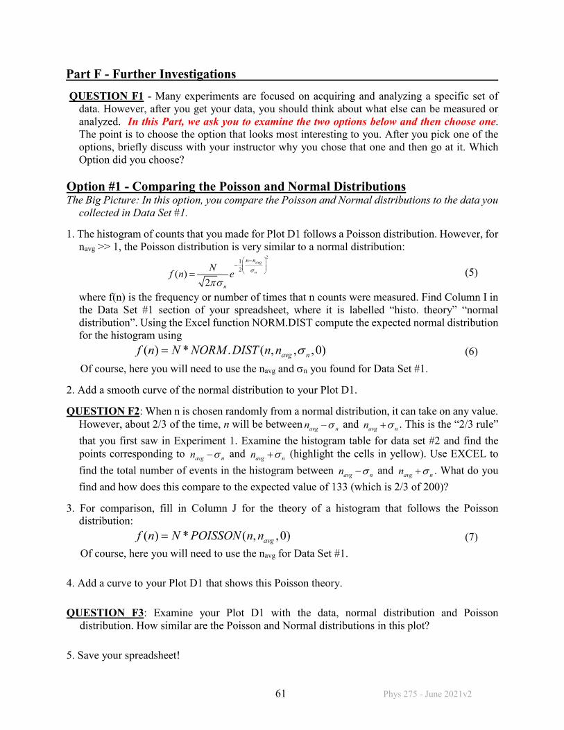
collected in Data Set #1. 1. The histogram of counts that you made for Plot D1 follows a Poisson distribution. However, for

navg >> 1, the Poisson distribution is very similar to a normal distribution:

2

12( )

2

avg

n

n n

n

Nf n e σ

πσ

−−

= (5)

where f(n) is the frequency or number of times that n counts were measured. Find Column I in the Data Set #1 section of your spreadsheet, where it is labelled “histo. theory” “normal distribution”. Using the Excel function NORM.DIST compute the expected normal distribution for the histogram using

( ) * . ( , , ,0)avg nf n N NORM DIST n n σ= (6) Of course, here you will need to use the navg and σn you found for Data Set #1. 2. Add a smooth curve of the normal distribution to your Plot D1. QUESTION F2: When n is chosen randomly from a normal distribution, it can take on any value.

However, about 2/3 of the time, n will be between avg nn σ− and avg nn σ+ . This is the “2/3 rule” that you first saw in Experiment 1. Examine the histogram table for data set #2 and find the points corresponding to avg nn σ− and avg nn σ+ (highlight the cells in yellow). Use EXCEL to find the total number of events in the histogram between avg nn σ− and avg nn σ+ . What do you find and how does this compare to the expected value of 133 (which is 2/3 of 200)?

3. For comparison, fill in Column J for the theory of a histogram that follows the Poisson

distribution: ( ) * ( , ,0)avgf n N POISSON n n= (7) Of course, here you will need to use the navg for Data Set #1. 4. Add a curve to your Plot D1 that shows this Poisson theory. QUESTION F3: Examine your Plot D1 with the data, normal distribution and Poisson

distribution. How similar are the Poisson and Normal distributions in this plot? 5. Save your spreadsheet!

62 Phys 275 - June 2021v2

n avgnσ =Option #2 - Does ?

In this part you will quickly collect some more data and then make a plot that shows the most important property of the Poisson distribution, which is that . 1. Data Set #4 – Background counts To measure background counts, lift the Digital Radiation Monitor off the source tray and

move the source tray about 1 to 2 meters away from the DRM. Collect counts for a total Duration of 200 s using a sampling rate of 1 sample/second (1 s counting interval). Copy and paste the background counts data into the designated area in your spreadsheet.

You should see that the Geiger counter detects counts even when the source is not present! These “background counts” are from cosmic rays and the decay of radioactive nuclei that are naturally present in small amounts in everyday materials. If you need an accurate measurement of the strength of a weak source, you would need to subtract these background counts. Since you don't need an accurate measurement of the source strength in this lab, we have not asked you to subtract the background level from your source measurements. Here we just want you to see how big the background level is.

2. Data Set #5 - Source Counts with 10 samples/s or 0.1 second counting interval Replace the source so it is under the DRM. Set the counter to collect data for a Duration of 20

s with a sampling rate of 10 samples per second (0.5 s counting interval). Copy all the time and counts data into the designated area in your spreadsheet. There should be N =200 data points.

3. Data Set #6 - Source Counts with 100 samples/s 0.01 second counting interval With source still under the detector, set the counter to collect data for a Duration of 20 s with a

sampling rate of 100 samples per second (0.01 s counting interval). Copy all the time and counts data into the designated area in your spreadsheet. There should be N =2000 data points.

4. Save your Spreadsheet. 5. In the designated cells for Data Sets #4, #5 and #6, use EXCEL to find: the number of measurements: N average number of counts: navg square root of the number of counts: avgn standard deviation in the number of counts: σn uncertainty in the average (also called standard error in the mean): /navg n Nσ σ= uncertainty in the standard deviation of the number of counts: / 2( 1)n Nσσ σ= − .

6. By this step, you should have found navg and σn for all six Data Sets (#1 to #6). The template collects these results and many others into a convenient table near cell BL12. Find this table in Part F of your spreadsheet. Note that there is also a column for the “smooth theory curve” where we found the theoretically expected result at a large number of points so that it will make a smooth curve on a plot.

Plot F. The template has a nice plot showing the theory . Find Plot F and add to it your measured results for σn versus navg from Data Sets #1 to #6. Add error bars. Note: there are uncertainties in your measured values of navg (the x-axis) and

σn (the y-axis) and these have been collected into the table by the template.

n avgnσ =

n avgnσ =

n avgnσ =

63 Phys 275 - June 2021v2

Question F4: Does your data appear to be consistent with the theory that ? VIII. Finishing Up

Save your spreadsheet and submit it to ELMS before you leave the Lab.

Turn in your checksheet to your instructor before you leave.

If you did not complete the entire lab in class, finish everything at home and submit a revised spreadsheet to ELMS before the start of your next lab.

If you finished early, use the remaining class time to work on the homework.

IX. Homework (Submit your answers to the homework to Expert TA before the deadline) Questions and multiple choice answers on Expert TA may vary from those given below. Be sure

to read questions and choices carefully before submitting your answers on Expert TA.

#1. A radioactive sample has 1020 atoms in it. Assume each atom has a mean lifetime of 3*1016 s (about 1 billion years). (a) On average, how many decays will there be in 1 s. (b) What is the standard deviation in the number of decays?

#2. In one second, a student measures 80 counts from a radioactive sample and concludes that it is

decaying at a steady average rate of 80 counts per second. Based on this one measurement, and the fact that this random decay process obeys Poisson statistics, what is the uncertainty in the count rate in counts per second?

#3. Suppose you measure a radioactive source and find an average of 20 counts in a 1 second

interval. According to the Poisson distribution, what is the probability of seeing 0 counts during a 1 s interval?

#4. Two students are measuring radioactive decays from two identical samples using identical

detectors. One student measures decays for one second and finds n1 = 1000 counts, while the other student measures for one second and finds n2 = 1100 counts. This problem involves figuring out if this difference in measured results is statistically significant, or if the difference can be attributed to the random nature of the decay process. To answer this question quantitatively, you need to do a χ2 analysis. To do this, note that

(n2-n1)data = 100 Assume as a theory that the sources are the same so that the difference in counts is zero: (n2-n1)theory = 0.

(a) For n1 = 1000 and n2 = 1100, use propagation of errors to find the expected uncertainty in n2-n1 due to Poisson statistical fluctuations in the number of decays.

(b) Calculate χ2 for this theory, data and uncertainty, (c) How many degrees of freedom are there? (d) Use EXCEL’s chidist function to calculate P(χ2,v). (e) Do the two measurements disagree significantly?

#5H. [This Question is for Hotshots Only]. Take another look at your answer to question C4.

Explain in detail why there is such a big discrepancy between the expected decay rate and what

n avgnσ =

64 Phys 275 - June 2021v2

your G.M. tube measured. Hint: What does the Cs-137 release when it decays? Which decay products are detected? Why aren’t the other decay products detected?

#6H. [This Question is for Hotshots Only]. Suppose you measure 0 background counts in a 1 s

interval. Clearly your best estimate for the background count rate is 0 per second, but what would be the uncertainty in this estimate? Explain.

#7H. [This Question is for Hotshots Only]. Prove that the mean life τ and the half-life τ1/2 are related by τ = τ1/2/ln(2).

#8H. [This Question is for Hotshots Only]. The mean life of Cs-137 is τ =43.5 years and the Cs-137 source has a strength of 1 µCi. How many Cs-137 atoms are there in the source? What is the total mass of the Cs-137 atoms in the source?