Embed Size (px)
Citation preview

© 2007 Emona Instruments Experiment 21 – DSSS modulation & demodulation 21-2
Experiment 21 – DSSS modulation and demodulation
Preliminary discussion
Recall that when a sinusoidal carrier is DSBSC modulated by a message, the two signals are
multiplied together. Recall also that the resulting DSBSC signal consists of two sets of
sidebands but no carrier (refer to the preliminary discussion of Experiment 6 for a discussion
of this).
When the DSBSC signal is demodulated using product detection, both sidebands are multiplied
with a local carrier that must be synchronised to the transmitter’s carrier (that is, it has the
same frequency and phase). Doing so produces two messages that are in-phase with each other
and so add to form a single bigger message (refer to the preliminary discussion of Experiment
9 for a discussion of this).
Direct sequence spread spectrum (DSSS or often just “spread spectrum”) is a variation of the
DSBSC modulation scheme with a pulse train (called a pseudo-noise sequence or just PN
sequence) for the carrier instead of a simple sinewave. This may sound radical until you
remember that pulse trains are actually made up of a theoretically infinite number of
sinewaves (the fundamental and harmonics). That being the case, spread spectrum is really the
DSBSC modulation of a theoretically infinite number of sinusoidal carrier signals. The result is
a theoretically infinite number of pairs of tiny sidebands about a suppressed carrier.
In practice, not all of these sidebands have any energy of significance. However, the fact that
the message information is distributed across so many of them makes spread spectrum signals
difficult to deliberately interfere with or “jam”. To do so, you would have to upset a significant
number of the sidebands which is difficult considering their number.
Spread spectrum signals are demodulated in the same way as DSBSC signals using a product
detector. Importantly, the product detector’s local carrier signal must contain all the
sinewaves that make up transmitter’s pulse train at the same frequency and phase. If this is
not done, the tiny demodulated signals will be at the wrong frequency and phase and so they
won’t add up to reproduce the original message. Instead, they’ll produce a garbage signal that
looks like noise.
The only way for the receiver to generate the right number of sinewaves at the right
frequency is to use a pulse train with an identical sequence to that used by the transmitter.
Moreover, it must be synchronised. This issue gives spread spectrum another of its advantages
over other modulation schemes. The transmitted signal is effectively encrypted.
Of course, with trial and error it’s possible for an unauthorised person to guess the correct PN
sequence to use for their receiver. However, this can be made difficult by making the
sequence longer before it repeats itself (that is, by making it consist of more bits or chips).
Longer sequences can produce more combinations of unique codes which would take longer to
guess using a trial and error approach. To illustrate this point, an 8-bit code has 256
combinations while a 20-bit code has 1,048,575 combinations. A 256-bit code has 1.1579×1077
combinations. That’s 11579 with 73 zeros after it!

Experiment 21 – DSSS modulation & demodulation © 2007 Emona Instruments 21-3
Increasing the sequence’s chip-length has another advantage. To explain, the total energy in a
spread spectrum signal is distributed between all of the tiny DSBSC that make it up (though
not evenly because not all of the sinewaves that make up the carrier’s pulse train are the same
amplitude). A mathematical technique called Fourier Analysis shows that the greater the
number of chips in a sequence before repeating, the greater the number of sinewaves of
significance needed to make it.
That being the case, using more chips in the transmitter’s PN sequence produces more DSBSC
signals and so the signal’s total energy is distributed more thinly between them. This in turn
means that the individual signals are many and extremely small. In fact, if the PN sequence is
long enough, all of these DSBSC signals are smaller than the background electrical noise that’s
always present in free-space. This fact gives spread spectrum yet another important
advantage. The signal is difficult to detect.
Spread spectrum finds use in several digital applications including: CDMA mobile phone
technology, cordless phones, the global positioning system (GPS) and two of the 802.11 wi-fi
standards.
The experiment
In this experiment you’ll use the Emona DATEx to generate a DSSS signal by implementing its
mathematical model. You’ll then use a product detector (with a stolen carrier) to reproduce
the message. Once done, you’ll examine the importance of using the correct PN sequence for
the local carrier and the difficulty of jamming DSSS signals.
It should take you about 50 minutes to complete this experiment.
Equipment
� Personal computer with appropriate software installed
� NI ELVIS plus connecting leads
� NI Data Acquisition unit such as the USB-6251 (or a 20MHz dual channel oscilloscope)
� Emona DATEx experimental add-in module
� two BNC to 2mm banana-plug leads
� assorted 2mm banana-plug patch leads

© 2007 Emona Instruments Experiment 21 – DSSS modulation & demodulation 21-4
Procedure
Part A – Generating a DSSS signal using a simple message
As DSSS is basically just DSBSC with a pulse train for the carrier instead of a simple sinusoid,
it can be generated by implementing the mathematical model for DSBSC.
1. Ensure that the NI ELVIS power switch at the back of the unit is off.
2. Carefully plug the Emona DATEx experimental add-in module into the NI ELVIS.
3. Set the Control Mode switch on the DATEx module (top right corner) to PC Control.
4. Check that the NI Data Acquisition unit is turned off.
5. Connect the NI ELVIS to the NI Data Acquisition unit (DAQ) and connect that to the
personal computer (PC).
6. Turn on the NI ELVIS power switch at the back then turn on its Prototyping Board Power switch at the front.
7. Turn on the PC and let it boot-up.
8. Once the boot process is complete, turn on the DAQ then look or listen for the
indication that the PC recognises it.
9. Launch the NI ELVIS software.
10. Launch the DATEx soft front-panel (SFP) and check that you have soft control over the
DATEx board.
11. Locate the Sequence Generator module on the DATEx SFP and set its soft dip-switches
to 00.

Experiment 21 – DSSS modulation & demodulation © 2007 Emona Instruments 21-5
12. Connect the set-up shown in Figure 1 below.
Note: Insert the black plugs of the oscilloscope leads into a ground (GND) socket.
Figure 1
This set-up can be represented by the block diagram in Figure 2 below. It multiplies the 2kHz
sinewave message with a PN sequence modelled by the Sequence Generator’s 32-bit pulse train
output.
Figure 2
MASTERSIGNALS
100kHzSINE
100kHzCOS
100kHzDIGITAL
8kHzDIGITAL
2kHzSINE
2kHzDIGITAL
SCOPECH A
CH B
TRIGGER
1
O
SPEECH
SEQUENCEGENERATOR
GND
GND
SYNC
CLK
LINECODE
X
Y
OO NRZ-L
O1 Bi-O
1O RZ-AMI
11 NRZ-M
MULTIPLIER
X DC
Y DC kXY
SERIAL X1
X2CLK
SERIAL TOPARALLEL
S/ P
Message
To Ch.AMaster
Signals
Master
Signals
DSSS signal
To Ch.B2kHz
Multiplier
module
100kHz
CLK
Sequence
Generator
PN sequence

© 2007 Emona Instruments Experiment 21 – DSSS modulation & demodulation 21-6
13. Set up the scope per the instructions in Experiment 1 with the following changes:
� Timebase control to 100µs/div instead of 500µs/div
� Channel B Scale control to 2V/div instead of 1V/div
14. Activate the scope’s Channel B input to observe the DSSS signal out of the Multiplier
module as well as the message signal.
15. Draw the two waveforms to scale in the space provided below leaving room to draw a
third waveform.
Tip: Draw the message signal in the upper third of the graph and the DSSS signal in the
middle third.

Experiment 21 – DSSS modulation & demodulation © 2007 Emona Instruments 21-7
Question 1
What feature of the Multiplier module’s output suggests that it’s basically a DSBSC
signal? Tip: If you’re not sure, read the preliminary discussion for Experiment 6.
Question 2
Why is the DSSS signal so large when it’s supposed to be small and indistinguishable
from noise? Tip: If you’re not sure, see the preliminary discussion for this experiment.
Ask the instructor to check
your work before continuing.

© 2007 Emona Instruments Experiment 21 – DSSS modulation & demodulation 21-8
Part B – Observations of DSSS signals in the frequency domain
One of the features of DSSS is that it produces a theoretically infinite number of pairs of
tiny sidebands with each pair straddling a suppressed carrier. This part of the experiment lets
you examine this.
16. Slide the NI ELVIS Function Generator’s Control Mode switch so that it’s no-longer in
the Manual position.
17. Launch the Function Generator’s VI.
18. Press the Function Generator VI’s ON/OFF control to turn it on.
19. Adjust the Function Generator using its soft controls for an output with the following
specifications:
� Waveshape: Square
� Frequency: 30kHz
� Amplitude: 4Vp-p
� DC Offset: 0V
20. Disconnect the plug to the Sequence Generator module’s LINE CODE output and modify
the set-up as shown in Figure 3 below.
Figure 3
21. Examine the new DSSS signal on the scope.
Note: You should notice that it looks similar to the DSSS signal you obtained earlier.
That said, it’ll be different in that the spacing between the carrier’s transitions are
regular.
MASTERSIGNALS
100kHzSINE
100kHzCOS
100kHzDIGITAL
8kHzDIGITAL
2kHzSINE
2kHzDIGITAL
SCOPECH A
CH B
TRIGGER
1
O
SPEECH
SEQUENCEGENERATOR
GND
GND
SYNC
CLK
LINECODE
X
Y
OO NRZ-L
O1 Bi-O
1O RZ-AMI
11 NRZ-M
MULTIPLIER
X DC
Y DC kXY
SERIAL X1
X2CLK
SERIAL TOPARALLEL
S/ P
VARIABLE DC
FUNCTIONGENERATOR
+
ANALOG I/ O
ACH1 DAC1
ACH0 DAC0
Experiment 21 – DSSS modulation & demodulation © 2007 Emona Instruments 21-9
The set-up in Figure 3 can be represented by the block diagram in Figure 4 below. Notice that
the carrier signal is a 30kHz squarewave.
Figure 4
Recall that a squarewave consists of a fundamental at the same frequency as the squarewave
itself and a theoretically infinite number of odd harmonics (each with proportionally smaller
amplitude to the amplitude of the frequency before it). So, our 30kHz squarewave carrier
consists of sinewaves at 30kHz, 90kHz, 150kHz, 210kHz and so on.
Theoretically then, the DSSS signal consists of a 30kHz suppressed carrier with 28kHz and
32kHz lower and upper sidebands, a 90kHz suppressed carrier with 88kHz and 92kHz lower
and upper sidebands, a 150kHz suppressed carrier with 148kHz and 152kHz lower and upper
sidebands, and so on. Let’s examine these using the NI ELVIS Dynamic Signal Analyzer virtual
instrument.
Message
To Ch.AMaster
Signals
DSSS signal
To Ch.B2kHz
Multiplier
module
Function
Generator
30kHz squarewave
© 2007 Emona Instruments Experiment 21 – DSSS modulation & demodulation 21-10
22. Suspend the scope VI’s operation by pressing its RUN control once.
Note: The scope’s display should freeze.
23. Launch the NI ELVIS Dynamic Signal Analyzer VI.
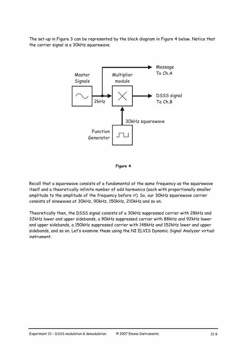
24. Adjust the Signal Analyzer’s controls as follows:
General
Sampling to Run
Input Settings
� Source Channel to Scope CHB
FFT Settings
� Frequency Span to 200,000
� Resolution to 400
� Window to 7 Term B-Harris
Triggering
� Triggering to Immediate
Frequency Display
� Units to dB
� RMS/Peak to RMS
� Scale to Auto
� Voltage Range to ±10V
Averaging
� Mode to RMS
� Weighting to Exponential � # of Averages to 3
� Markers to OFF (for now)
The display should now be showing about ten pairs of what appear to be significant sinewaves.
This is deceptive as you’ll see.
25. Activate the Signal Analyzer’s markers by pressing the Markers button.
26. Use the Signal Analyzer’s M1 marker to measure the frequency in the middle of each
pair of the sinewaves.
Note: You’ll find that the signal consists of pairs of sidebands about a suppressed
carrier at frequencies listed in the second last paragraph of the previous page.
You’ll also find that it consists of sidebands about suppressed carriers at other
frequencies. However, although these signals are present, the display is a little
misleading because the vertical axis is logarithmic (i.e. non-linear).

Experiment 21 – DSSS modulation & demodulation © 2007 Emona Instruments 21-11
27. Change the Signal Analyzer’s Units control (under the Frequency Display heading) from
dB to Linear.
Note: This display shows you the linear relationship between the sinewaves’ amplitude.
28. Use the Signal Analyzer’s M1 marker to measure the frequency of these significant
sinewaves.
Note: The frequencies should be identical to those listed on the bottom of page 21-9.
29. Return the Signal Analyzer’s Units control to the dB position.
30. Disconnect the patch lead from the Function Generator’s output and return it to the
Sequence Generator module’s LINE Code output.
Note: This returns the set-up to that shown in Figures 1 and 2 with a PN Sequence for
the carrier instead of a squarewave.
31. Examine the spectral composition of the original DSSS signal with the Signal Analyzer’s
Units control in both the dB and Linear positions.
Question 3
Why is the spectral composition of the DSSS signal much more complex when the
carrier is a PN Sequence instead of a squarewave?
Ask the instructor to check
your work before continuing.

© 2007 Emona Instruments Experiment 21 – DSSS modulation & demodulation 21-12
Part C – Using the product detector to recover the message
32. Close the Signal Analyzer’s VI.
33. Restart the scope’s VI by pressing its RUN control once.
34. Set up the scope per the instructions in Experiment 1 with the following changes:
� Timebase control to 100µs/div instead of 500µs/div
� Channel B Scale control to 2V/div instead of 1V/div
� Activate the scope’s Channel B input
35. Locate the Tuneable Low-pass Filter module on the DATEx SFP and set its soft Gain
control to about a quarter of its travel.
36. Turn the Tuneable Low-pass Filter module’s soft Cut-off Frequency Adjust control fully
anti-clockwise.
37. Disconnect the plugs to the Speech module’s output and modify the set-up as shown in
Figure 5 below.
Note: Notice that the leads connect to the Multiplier module’s AC inputs and not its DC
inputs.
Figure 5
MASTERSIGNALS
100kHzSINE
100kHzCOS
100kHzDIGITAL
8kHzDIGITAL
2kHzSINE
2kHzDIGITAL
SCOPECH A
CH B
TRIGGER
1
O
SPEECH
SEQUENCEGENERATOR
GND
GND
SYNC
CLK
LINECODE
X
Y
OO NRZ-LO1 Bi-O
1O RZ-AMI11 NRZ-M
MULTIPLIER
X DC
Y DC kXY
SERIAL X1
X2CLK
SERIAL TOPARALLEL
S/ P
fC
x100
fC
GAIN
IN OUT
TUNEABLELPF
Y
DC
AC
MULTIPLIER
MULTIPLIER
kXY
X DC
Y DC kXY
DC
XAC
Experiment 21 – DSSS modulation & demodulation © 2007 Emona Instruments 21-13
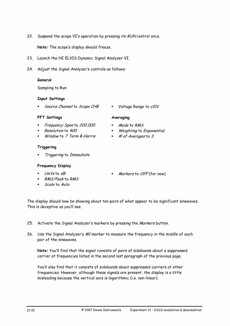
The additions to the set-up in Figure 5 can be represented by the block diagram in Figure 6
below. The Multiplier module and the Tuneable Low-pass Filter module implement a product
detector which recovers the original message from the DSSS signal. To facilitate this, the PN
sequence used for the modulator’s carrier is “stolen” for the product detector’s local carrier
(though it’s stolen from the module’s X output but the bit pattern is the same).
Figure 6
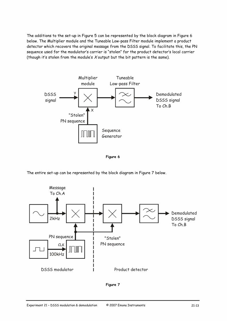
The entire set-up can be represented by the block diagram in Figure 7 below.
Figure 7
DSSS
signal
Y
X
Demodulated
DSSS signal
To Ch.B
Multiplier
module
Tuneable
Low-pass Filter
Sequence
Generator
"Stolen"
PN sequence
Message
To Ch.A
Demodulated
DSSS signal
To Ch.B
2kHz
100kHz
CLK
PN sequence "Stolen"
PN sequence
DSSS modulator Product detector

© 2007 Emona Instruments Experiment 21 – DSSS modulation & demodulation 21-14
38. Slowly turn the Tuneable Low-pass Filter module’s soft Cut-off Frequency control
clockwise while watching the scope’s display.
Remember: You can use the keyboard’s TAB and arrow keys for fine adjustments of
DATEx controls.
39. Stop when the message signal has been recovered and is about in phase with the original.
40. Draw the demodulated DSSS signal to scale in the space that you left on the graph
paper.
Recall that the message can only be recovered by the product detector if an identical PN
sequence to the DSSS modulator’s carrier is used. The next part of the experiment
demonstrates this.
41. Modify the set-up as shown in Figure 8 below to make the demodulator’s local carrier a
different PN sequence to the transmitter’s carrier.
Figure 8
Ask the instructor to check
your work before continuing.
MASTERSIGNALS
100kHzSINE
100kHzCOS
100kHzDIGITAL
8kHzDIGITAL
2kHzSINE
2kHzDIGITAL
SCOPECH A
CH B
TRIGGER
1
O
SPEECH
SEQUENCEGENERATOR
GND
GND
SYNC
CLK
LINECODE
X
Y
OO NRZ-LO1 Bi-O
1O RZ-AMI11 NRZ-M
MULTIPLIER
X DC
Y DC kXY
SERIAL X1
X2CLK
SERIAL TOPARALLEL
S/ P
fC
x100
fC
GAIN
IN OUT
TUNEABLELPF
Y
DC
AC
MULTIPLIER
MULTIPLIER
kXY
X DC
Y DC kXY
DC
XAC

Experiment 21 – DSSS modulation & demodulation © 2007 Emona Instruments 21-15
42. Compare the message with the product detector’s new output.
Question 4
What does the signal out of the low-pass filter look like?
Question 5
Why does using the wrong PN sequence for the local carrier cause the product
detector’s output to look like this?
Part D - DSSS and deliberate interference (jamming)
Interference occurs when an unwanted electrical signal gets added to the transmitted signal
(typically in the channel) and changes it enough to change the recovered message. Electrical
noise is a significant source of unintentional interference.
However, sometimes noise is deliberately added to the transmitted signal for the purpose of
interfering or “jamming” it. The next part of the experiment models deliberate interference
to show how spread spectrum signals are highly resistant to it.
43. Move the patch lead from the Sequence Generator’s Y output back to its X output.
Note: The product detector should now be recovering the message again.
Ask the instructor to check
your work before continuing.

© 2007 Emona Instruments Experiment 21 – DSSS modulation & demodulation 21-16
44. Adjust the Function Generator using its soft controls for an output with the following
specifications:
� Waveshape: Sine
� Frequency: 50kHz
� Amplitude: 4Vp-p
� DC Offset: 0V
45. Set the scope’s Trigger Source control to the CH B position.
46. Locate the Adder module on the DATEx SFP and turn its soft g control fully anti-
clockwise.
47. Set the Adder module’s soft G control to about the middle of its travel.
48. Modify the set-up as shown in Figure 9 below.
Figure 9
MASTERSIGNALS
100kHzSINE
100kHzCOS
100kHzDIGITAL
8kHzDIGITAL
2kHzSINE
2kHzDIGITAL
SCOPECH A
CH B
TRIGGER
1
O
SPEECH
SEQUENCEGENERATOR
GND
GND
SYNC
CLK
LINECODE
X
Y
OO NRZ-LO1 Bi-O1 O RZ-AMI1 1 NRZ-M
MULTIPLIER
X DC
Y DC kXY
SERIAL X1
X2CLK
SERIAL TOPARALLEL
S/ P
fC
x10 0
fC
GAIN
IN OUT
TUNEABLELPF
Y
DC
AC
MULTIPLIER
MULTIPLIER
kXY
X DC
Y DC kXY
DC
XAC
B
A
ADDER
G
GA+gB
g
VARIABLE DC
FUNCTIONGENERATOR
+
ANALOG I/ O
ACH1 DAC1
ACH0 DAC0
Experiment 21 – DSSS modulation & demodulation © 2007 Emona Instruments 21-17
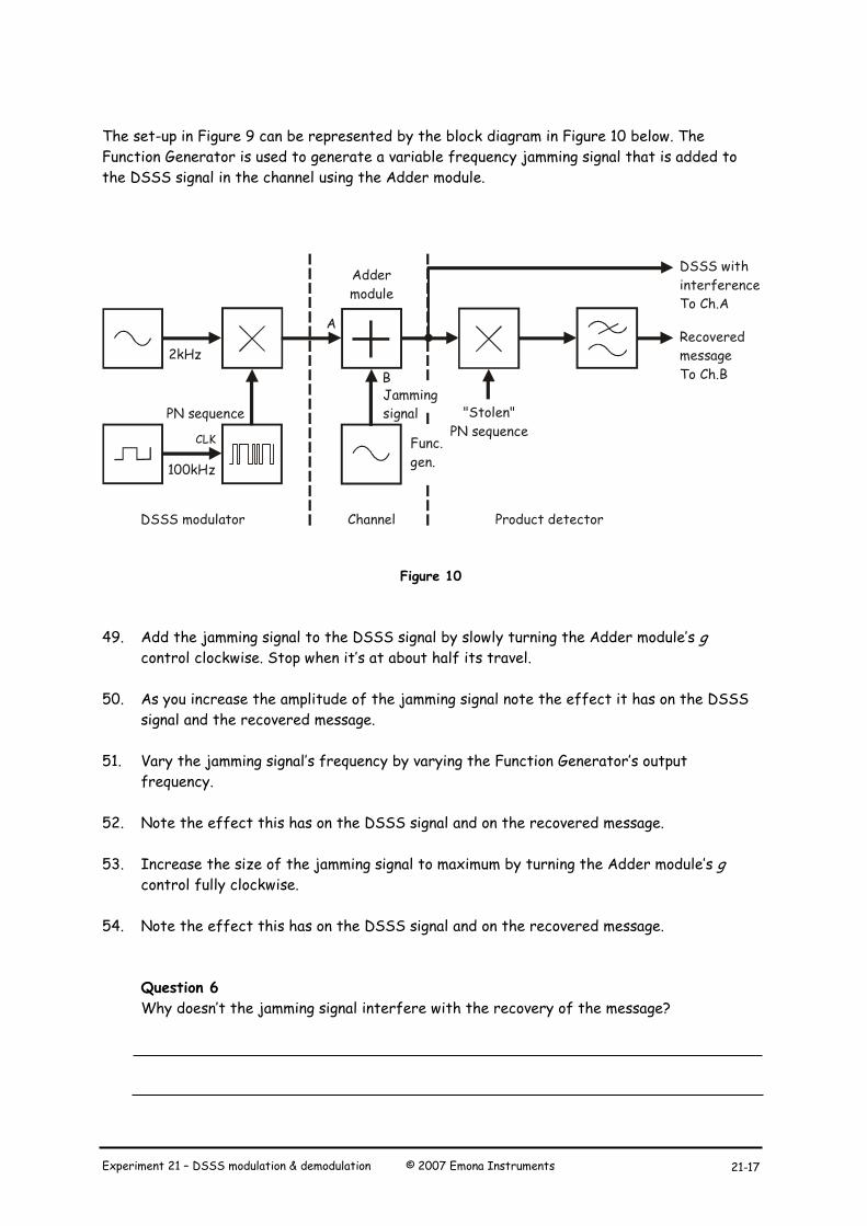
The set-up in Figure 9 can be represented by the block diagram in Figure 10 below. The
Function Generator is used to generate a variable frequency jamming signal that is added to
the DSSS signal in the channel using the Adder module.
Figure 10
49. Add the jamming signal to the DSSS signal by slowly turning the Adder module’s g
control clockwise. Stop when it’s at about half its travel.
50. As you increase the amplitude of the jamming signal note the effect it has on the DSSS
signal and the recovered message.
51. Vary the jamming signal’s frequency by varying the Function Generator’s output
frequency.
52. Note the effect this has on the DSSS signal and on the recovered message.
53. Increase the size of the jamming signal to maximum by turning the Adder module’s g
control fully clockwise.
54. Note the effect this has on the DSSS signal and on the recovered message.
Question 6
Why doesn’t the jamming signal interfere with the recovery of the message?
DSSS with
interference
To Ch.A
Recovered
message
To Ch.B
2kHz
100kHz
CLK
PN sequence "Stolen"
PN sequence
DSSS modulator Product detector
A
B
Adder
module
Channel
Jamming
signal
Func.
gen.

© 2007 Emona Instruments Experiment 21 – DSSS modulation & demodulation 21-18
each individual DSBSC signal contributes so little to the final output signal.
A more sophisticated approach to jamming involves automatically sweeping the jamming signal
through a wide range of frequencies to increase the chances of upsetting the transmitted
signal. The next part of the experiment let’s you see how spread spectrum handles this.
55. Return the Adder module’s g control to about the middle of its travel.
56. Modify the set-up as shown in Figure 11 below.
Figure 11
This modification forces the Function Generator’s output to sweep continuously through a wide
range of frequencies.
Ask the instructor to check
your work before continuing.
MASTERSIGNALS
100kHzSINE
100kHzCOS
100kHzDIGITAL
8kHzDIGITAL
2kHzSINE
2kHzDIGITAL
SCOPECH A
CH B
TRIGGER
1
O
SPEECH
SEQUENCEGENERATOR
GND
GND
SYNC
CLK
LINECODE
X
Y
OO NRZ-LO1 Bi-O1O RZ-AMI11 NRZ-M
MULTIPLIER
X DC
Y DC kXY
SERIAL X1
X2CLK
SERIAL TOPARALLEL
S/ P
fC
x100
fC
GAIN
IN OUT
TUNEABLELPF
Y
DC
AC
MULTIPLIER
MULTIPLIER
kXY
X DC
Y DC kXY
DC
XAC
B
A
ADDER
G
GA+gB
g
VARIABLE DC
FUNCTIONGENERATOR
+
ANALOG I/ O
ACH1 DAC1
ACH0 DAC0

Experiment 21 – DSSS modulation & demodulation © 2007 Emona Instruments 21-19
57. Note the effect this has on the DSSS signal and on the recovered message.
58. Increase the size of the jamming signal to maximum by turning the Adder module’s g
control fully clockwise.
59. Note the effect this has on the DSSS signal and on the recovered message.
Question 7
Why doesn’t the sweeping jamming signal interfere with the recovery of the message?
Ask the instructor to check
your work before continuing.
© 2007 Emona Instruments Experiment 21 – DSSS modulation & demodulation 21-20
An even more sophisticated approach to jamming involves using many jamming signals at once
(broadband jamming) to increase the chances of upsetting the transmitted signal. The next
part of the experiment let’s you see how spread spectrum handles this.
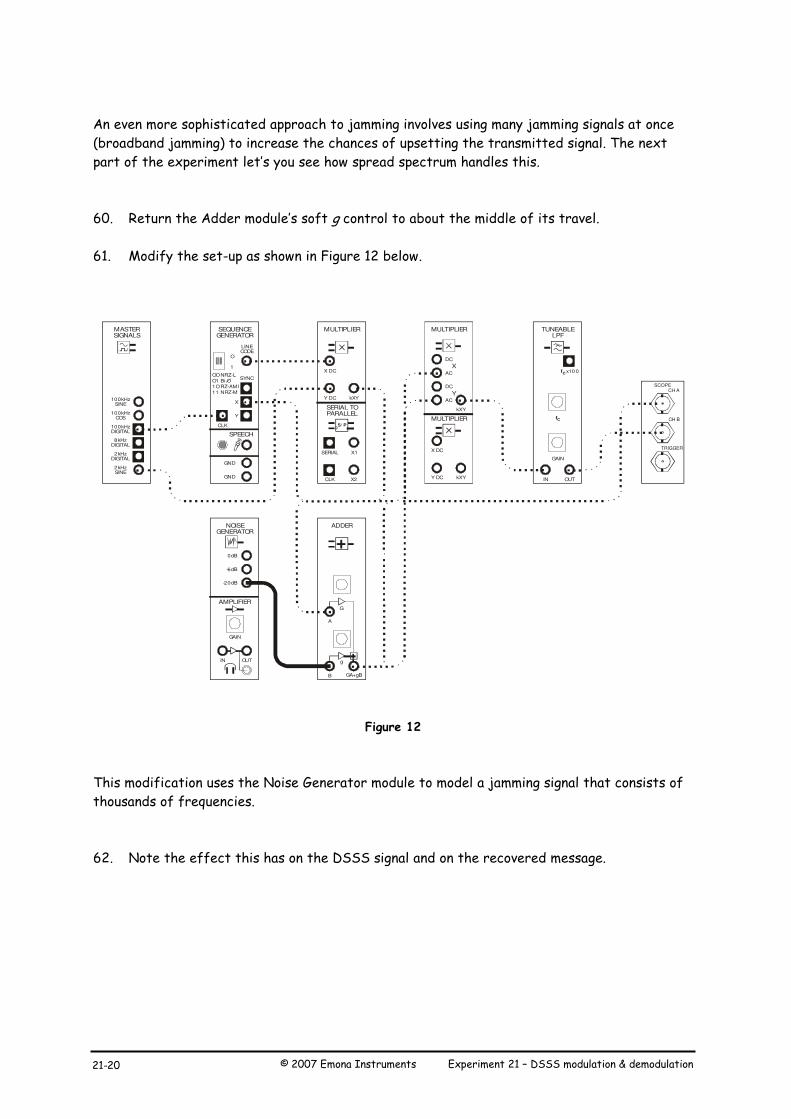
60. Return the Adder module’s soft g control to about the middle of its travel.
61. Modify the set-up as shown in Figure 12 below.
Figure 12
This modification uses the Noise Generator module to model a jamming signal that consists of
thousands of frequencies.
62. Note the effect this has on the DSSS signal and on the recovered message.
MASTERSIGNALS
100kHzSINE
100kHzCOS
100kHzDIGITAL
8kHzDIGITAL
2kHzSINE
2kHzDIGITAL
SCOPECH A
CH B
TRIGGER
1
O
SPEECH
SEQUENCEGENERATOR
GND
GND
SYNC
CLK
LINECODE
X
Y
OO NRZ-LO1 Bi-O1O RZ-AMI11 NRZ-M
MULTIPLIER
X DC
Y DC kXY
SERIAL X1
X2CLK
SERIAL TOPARALLEL
S/ P
fC
x10 0
fC
GAIN
IN OUT
TUNEABLELPF
Y
DC
AC
MULTIPLIER
MULTIPLIER
kXY
X DC
Y DC kXY
DC
XAC
B
A
ADDER
G
GA+gB
g
AMPLIFIER
GAIN
OUTIN
0dB
-6dB
-20dB
NOISEGENERATOR

Experiment 21 – DSSS modulation & demodulation © 2007 Emona Instruments 21-21
63. Increase the strength of the broadband jamming signal by connecting the Adder
module’s B input to the Noise Generator module’s -6dB output.
64. Note the effect this has on the DSSS signal and on the recovered message.
65. Increase the strength of the broadband jamming signal even more by connecting the
Adder module’s B input to the Noise Generator module’s 0dB output.
66. Note the effect this has on the DSSS signal and on the recovered message.
Question 8
Why doesn’t this broadband jamming signal interfere with the recovery of the message?
Ask the instructor to check
your work before finishing.
© 2007 Emona Instruments Experiment 21 – DSSS modulation & demodulation 21-22
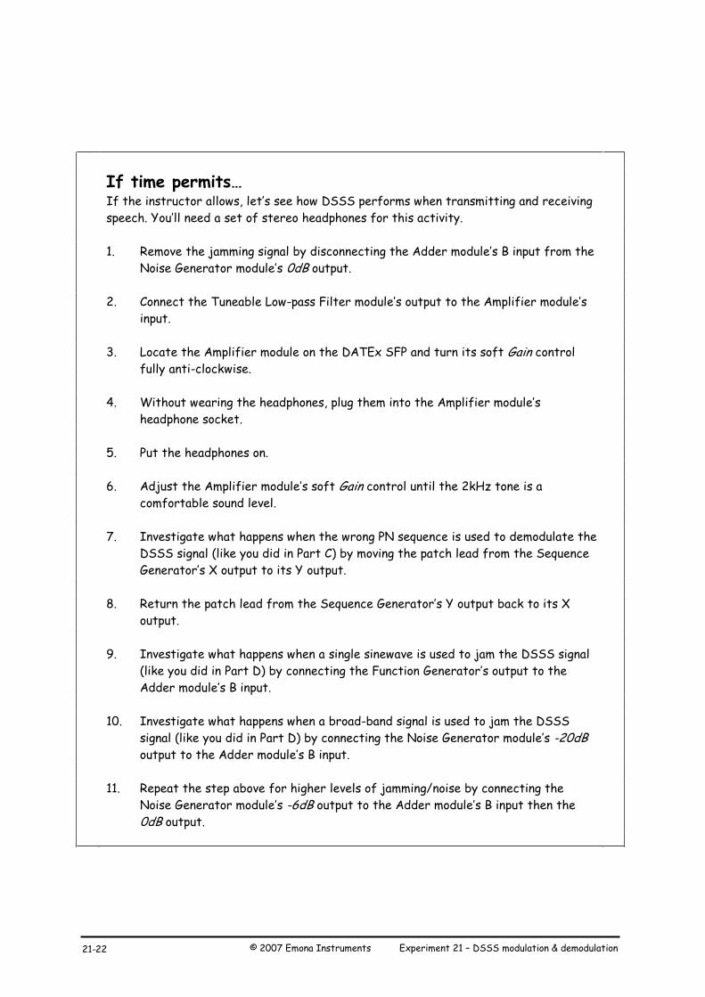
If time permits… If the instructor allows, let’s see how DSSS performs when transmitting and receiving
speech. You’ll need a set of stereo headphones for this activity.
1. Remove the jamming signal by disconnecting the Adder module’s B input from the
Noise Generator module’s 0dB output.
2. Connect the Tuneable Low-pass Filter module’s output to the Amplifier module’s
input.
3. Locate the Amplifier module on the DATEx SFP and turn its soft Gain control
fully anti-clockwise.
4. Without wearing the headphones, plug them into the Amplifier module’s
headphone socket.
5. Put the headphones on.
6. Adjust the Amplifier module’s soft Gain control until the 2kHz tone is a
comfortable sound level.
7. Investigate what happens when the wrong PN sequence is used to demodulate the
DSSS signal (like you did in Part C) by moving the patch lead from the Sequence
Generator’s X output to its Y output.
8. Return the patch lead from the Sequence Generator’s Y output back to its X
output.
9. Investigate what happens when a single sinewave is used to jam the DSSS signal
(like you did in Part D) by connecting the Function Generator’s output to the
Adder module’s B input.
10. Investigate what happens when a broad-band signal is used to jam the DSSS
signal (like you did in Part D) by connecting the Noise Generator module’s -20dB
output to the Adder module’s B input.
11. Repeat the step above for higher levels of jamming/noise by connecting the
Noise Generator module’s -6dB output to the Adder module’s B input then the
0dB output.