Embed Size (px)
Citation preview

“For External Distribution. © 2005 Halliburton. All Rights Reserved.”
EXPERIENCIA ACUMULADASEN LA COMPLETACIÓN YFRACTURAS DE POZOS
Jornada de Perforación, Terminación, Reparación y Servicio de PozosNeuquén, 15 de noviembre 2006

“For External Distribution. © 2005 Halliburton. All Rights Reserved.”
EXPERIENCIAS ACUMULADAS ENCOMPLETACIÓN Y FRACTURA DE POZOS.
AGENDA• DEVOLUCIÓN DE “PROPPANT”: REMEDIACIÓN
• DESARROLLO DE FORMACIONES TIGHT.
• FRACTURA CON COILED TUBING (COBRAMAX)
“For External Distribution. © 2005 Halliburton. All Rights Reserved.”
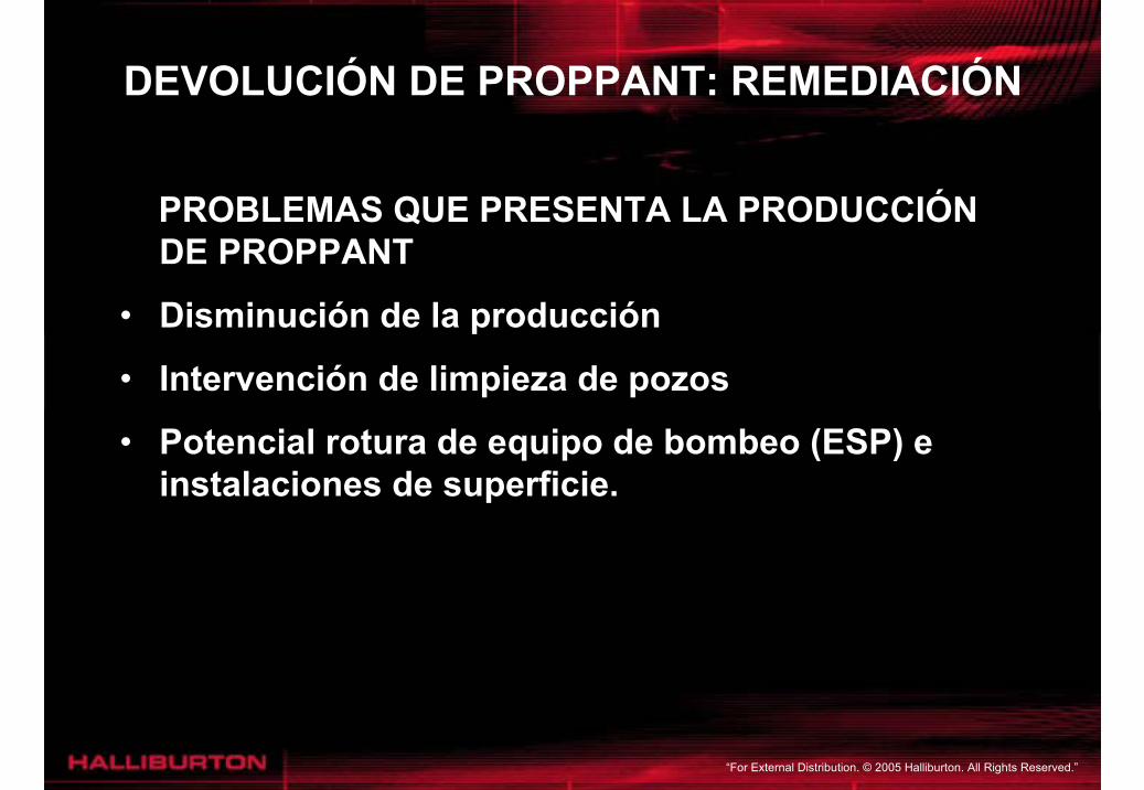
DEVOLUCIÓN DE PROPPANT: REMEDIACIÓN
PROBLEMAS QUE PRESENTA LA PRODUCCIÓNDE PROPPANT
• Disminución de la producción
• Intervención de limpieza de pozos
• Potencial rotura de equipo de bombeo (ESP) einstalaciones de superficie.

“For External Distribution. © 2005 Halliburton. All Rights Reserved.”
DEVOLUCIÓN DE PROPPANT: REMEDIACIÓN
CONTROL DE DEVOLUCIÓN DE ARENA:
TERMINACIÓN• Diseño de fractura• Cierre Forzado• Engravados• Agente de sostén resinados• Agente modificadores de la superficie del proppant• Fibras y termoplásticos.
REMEDIACIÓN• Disminución de caudal de producción• Inyección de resinas curables.

“For External Distribution. © 2005 Halliburton. All Rights Reserved.”
DEVOLUCIÓN DE PROPPANT: REMEDIACIÓN
TECNICAS DE COLOCACIÓN DE LAS RESINAS
• Bullheading
• Cañería con packer
• Coiled Tubing

“For External Distribution. © 2005 Halliburton. All Rights Reserved.”
DEVOLUCIÓN DE PROPPANT: REMEDIACIÓN
NUEVO MÉTODO DE TRATAMIENTO
“SISTEMA DE CONSOLIDACIÓN + NUEVA TÉCNICADE APLICACIÓN (COILED TUBING Y/O PACKER CON CAÑODE COLA + HERRAMIENTA DE PULSO DE PRESIÓN)”

“For External Distribution. © 2005 Halliburton. All Rights Reserved.”
DEVOLUCIÓN DE PROPPANT: REMEDIACIÓN
SISTEMA DE CONSOLIDACIÓN• Son sistemas de resinas líquidas cuya selección depende de
la temperatura de fondo de pozo.
• Se mezcla a la pasada y se inyecta para recubrir al agente desostén en la fractura
• No requieren catalizador
• El tiempo de curado es lento, lo que permite su colocaciónen forma adecuada.

“For External Distribution. © 2005 Halliburton. All Rights Reserved.”
DEVOLUCIÓN DE PROPPANT: REMEDIACIÓN
ETAPAS EN EL PROCESO DE CONSOLIDACIÓN• Preflujo 1: limpia el petróleo residual
• Preflujo 2: lava el petróleo y agua connata
• Separador: previene un curado prematuro
• Fluido de consolidación: resinas de baja viscosidad querecubre el agente de sostén consolidando sus granos.
• Separador: minimiza la contaminación de fluidos.
• Postflujo: remueve el exceso de resina en los poros.

“For External Distribution. © 2005 Halliburton. All Rights Reserved.”
DEVOLUCIÓN DE PROPPANT: REMEDIACIÓN
TRATAMIENTO TÍPICO CON CT• Limpiar cañería del CT
• Lavar el pozo con CT (gel + espumígeno + N2)
• Bombear tratamiento (Preflujos + Resinas + Postflujo)
• Desplazar el fluido de consolidación
• Sacar CT, con el anular del CT aun cerrado.
• Cerrar boca de pozo y bombear solución limpiadora del CT
• Mantener cerrado el pozo para el curado de la resina.

“For External Distribution. © 2005 Halliburton. All Rights Reserved.”
DEVOLUCIÓN DE PROPPANT: REMEDIACIÓN
“For External Distribution. © 2005 Halliburton. All Rights Reserved.”
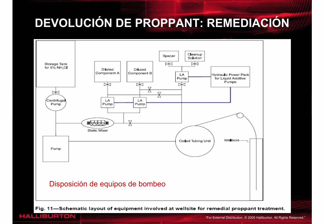
DEVOLUCIÓN DE PROPPANT: REMEDIACIÓN
Disposición de equipos de bombeo

“For External Distribution. © 2005 Halliburton. All Rights Reserved.”
DEVOLUCIÓN DE PROPPANT: REMEDIACIÓN
EXPERIENCIAS LOCALES

“For External Distribution. © 2005 Halliburton. All Rights Reserved.”
DEVOLUCIÓN DE PROPPANT:REMEDIACIÓN
EXPERIENCIAS LOCALES : RESULTADOS

“For External Distribution. © 2005 Halliburton. All Rights Reserved.”
DESARROLLO DE FORMACIONES TIGHTAGENDA
• Halliburton líder en desarrollo de Tight Sand
• Lecciones Aprendidas
• Implementación de soluciones

“For External Distribution. © 2005 Halliburton. All Rights Reserved.”
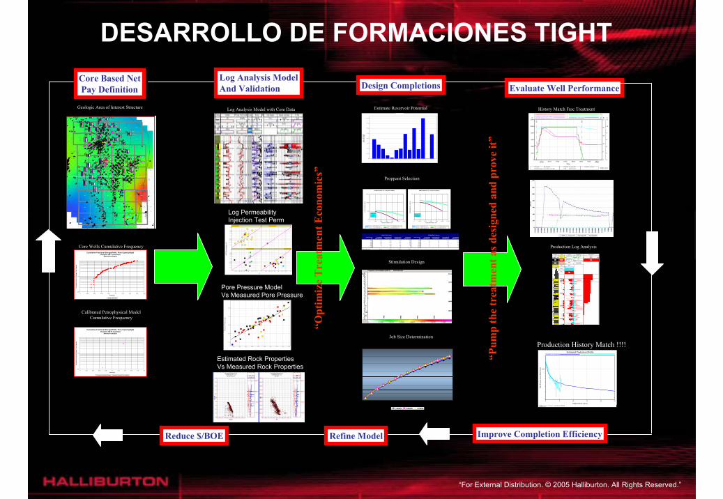
DESARROLLO DE FORMACIONES TIGHT
Cuales son las claves para producir lasreservas ?
• Proceso Sigma● Log análisis● Caracterización de reservorio● Selección de intervalo a punzar y fracturar● Análisis Económico● Ejecución de fractura● Evaluación de producción
“For External Distribution. © 2005 Halliburton. All Rights Reserved.”
DESARROLLO DE FORMACIONES TIGHT
Evaluate Well Performance
Estimated Production Profile
0 5 10 15 20 25
Elapsed Time (mon)
2
3
4
5
6
7
8
9
2
1000
Gas
Pro
duct
ion
(Msc
f/day
)
Predicted Gas Production Historical Gas Production
StiMRIL Forecast v2.7.0 beta 3�FracproPT and GOHFER21-Jul-03 14:52
4/2/200307:52 07:54 07:56 07:58 08:00 08:02 08:04
4/2/200308:06
Time
0
2000
4000
6000
8000
10000
12000A
0
5
10
15
20
25B
0
2
4
6
8
10
12C
Casing Pressure (psi) Slurry Rate (bpm)Proppant Concentration (lb/gal) GOHFER Bottom Hole Pressure (psi)GOHFER Surface Pressure (psi) GOHFER Slurry Rate (bpm)
A BC AA B
21
Customer: BP America Job Date: 02-Apr-2003 T icket #: 237223Well Description: Five Mile #19-3 Stg 1 UWI: 4903725293
StimWin v4.7.0a23-Apr-03 09:25
History Match Frac Treatment
Production History Match !!!!
Production Log Analysis
“Pum
p th
e tr
eatm
ent a
s des
igne
d an
d pr
ove
it”
Lithology
GR
0.000 300GAPI
Coal
Shale
Sandstone
Depth
GPAY
Net Pay
Rugose Hole
BHF
0 5
NPay
4 0
GPay
-4 4
Porosity
Core_Por(N/A)
0.25 0
COREPHI(N/A)
0.25 0
PHIE
0.25 0
BVW
0.25 0
Water
Gas
Permeability
DFIT Perm
0.0010 1V/V
KG_C
0.001 1
Perm to Gas
Flow Profile
QGSC
0 1500MF/D
Gas
10100
10200
10300
10400
Almond
MA 1
Summary – Total Well Production Job
Number Zone
Number Scenario Top
MD BottomMD
TreatmentVolume
ProppantAmount
Skin FractureLength
Avg Prop Conc
Fracture Conductivity
Linf
Qi
Qw
ft ft gal lb ft lb/ft² md*ft ft Mscf/day bpd 8 18 1 8943 8978 70922 216676 N/A 539 0.80 27 98.1 369 4.3 7 14 1 10156 10165 0 0 N/A 0 0.00 0 0.0 2 0.1 6 12 1 10262 10285 37496 79510 N/A 523 0.77 25 189.7 420 2.7 5 10 1 10317 10322 40592 85191 N/A 296 0.34 4 40.5 47 0.3 4 8 1 10352 10361 0 0 N/A 0 0.00 0 0.0 5 0.2 3 6 1 10414 10420 24372 61934 N/A 157 0.87 34 156.9 62 0.6 2 4 1 10444 10459 24232 2208 N/A 112 0.30 3 31.5 75 0.7 1 2 1 10493 10504 31890 21236 N/A 272 0.58 14 34.4 298 2.6
Total 1279 11.4
Reduce $/BOE Improve Completion EfficiencyRefine Model
Core Wells Cumulative Frequency
Calibrated Petrophysical ModelCumulative Frequency
Core Based Net Pay Definition
Cumulative Fractional Storage(PhiH) / Flow Capacity(KgH)Champlin 44A-1 (Core Data)
Almond Formation
0.01
0.1
1
0 0.02 0.04 0.06 0.08 0.1 0.12 0.14 0.16 0.18
Porosity %
Cum
ulat
ive
Frac
tiona
l Sto
rage
/ Fl
ow C
apac
ity
Series3 Series4
Cumulative Fractional Storage(PhiH) / Flow Capacity(KgH)Champlin 445-1A (Log Data)
Almond Formation
0.01
0.1
1
0 0.02 0.04 0.06 0.08 0.1 0.12 0.14 0.16 0.18 0.2
Porosity %
Cum
ulat
ive
Frac
tiona
l Sto
rage
/ Fl
ow C
apac
ity
Cumulative Fractional Storage Cumulative Frational Flow Capacity
Geologic Area of Interest Structure
Log Analysis ModelAnd Validation
Log Analysis Model with Core Data
���� _3�
���� ����� - � ��� ���
���� ����� - � � �� ���
���� ����� - ��� ��
���� ����� - � ��� ���
0.002 0.004 0.. . 0.. 0.01 0.02 0.04 0... 0.. 0.1 0.2 0.002 0.004 0... 0.. 0.01 0.02 0.04 0.. . 0. . 0.1 0.2
0.002
0.004
0.0060.0080.01
0.02
0.04
0.060.080.1
0.2
0.002
0.004
0.0060.0080.01
0.02
0.04
0.060.080.1
0.2
� ������� � ���� � �� ��� ���
8500 9000 9500 10000 10500 11000 11500 12000 12500 13000
4000
5000
6000
7000
8000
Log PermeabilityInjection Test Perm
Pore Pressure ModelVs Measured Pore Pressure
Estimated Rock PropertiesVs Measured Rock Properties
Estimate Reservoir Potential
“Opt
imiz
e T
reat
men
t Eco
nom
ics”
CONDUCTIVITY (md-ft) PERMEABILITY (Darcies)
Closure Stress 20/40PR6000 20/40INTERPROP 20/40SIN BAUX 20/40PR6000 Closure Stress 20/40PR6000 20/40INTERPROP 20/40SIN BAUX 20/40PR6000psi 0.9lb/sqft-210°F 0.9lb/sqft-210°F 0.9lb/sqft-210°F 0.9lb/sqft-210°F psi 0.9lb/sqft-210°F 0.9lb/sqft-210°F 0.9lb/sqft-210°F 0.9lb/sqft-210°F
2000 927 1242 1320 927 2000 111 173 189 1114000 670 1056 1106 670 4000 84 151 163 846000 390 785 925 390 6000 51 115 141 518000 176 588 701 176 8000 24 88 110 24
10000 76 445 480 76 10000 11 68 78 1112000 308 323 12000 49 54
Media n Dia m. (mm) 0.661 0.662 0.662 0.661
CONDUCTIVITY VS. CLOSURE STRESS
100
1000
10000
100000
0 2000 4000 6000 8000 10000 12000
CLOS URE S TRESS - PS I
CO
ND
UC
TIVI
TY M
D-F
T
0.9lb/sqft 20/40P R6000210°F 0.9lb/s qft 20/40INTERPROP 210°F0.9lb/sqft 20/40S IN BAUX210°F 0.9lb/s qft 20/40PR6000210°F
Stim-La b Inc.
P redKD99
PERMEABILITY VS. CLOS URE STRES S
1
10
100
1000
0 2000 4000 6000 8000 10000 12000
CLOSURE S TRES S - PSI
PER
MEA
BIL
ITY
- D
AR
CIE
S
0.9lb/s qft 20/40PR6000210°F 0.9lb/s qft 20/40INTERP ROP 210°F0.9lb/s qft 20/40SIN BAUX210°F 0.9lb/s qft 20/40P R6000210°F
Stim-La b Inc.P redKD99
Proppant Selection
Job Size NPV
0
200
400
600
800
1,000
1,200
1,400
Months
Dis
coun
ted
Cas
h Fl
ow
150000 180000 210000
Job Size Determination
Design Completions
� �� � ����
��� ����9756.75 9790.75 9831.75 9873.75 9888.75 9912.75 9923.75 9969.75 10009.... 10073.... 10100.... 10114.... 10177.... 10189....
0
2500
5000
7500
10000
12500
15000
17500
20000
Stimulation Design

“For External Distribution. © 2005 Halliburton. All Rights Reserved.”
DESARROLLO DE FORMACIONES TIGHTANALISIS DE PERFILES
� � �� � ������ � ��� �
� �� ����
0
1000
2000
3000
4000
5000
6000
7000
8000
9000
Grouping of OGIPfor Frac StageDesign
� � ��� � � � �� � ���� � �����
���
0 0.5 1 1.5 2 2.5 3 3.5 4
0
0.5
1
1.5
2
2.5
3
3.5

“For External Distribution. © 2005 Halliburton. All Rights Reserved.”
DESARROLLO DE FORMACIONES TIGHT– Relative Gas Permeability > 0.01 to 0.1 md– Porosity > 5% to 12%– Water Saturation > 35% to 60%– Pressure Gradient > 0.45 psi/ft to 0.53 psi/ft– Drainage Area :40 acres– EUR 1 to >10 BCF/well
0.001
0.010
0.100
1.000
0.00 0.02 0.04 0.06 0.08 0.10 0.12 0.14 0.16
core porosity, routine
core
per
mea
bilit
y

“For External Distribution. © 2005 Halliburton. All Rights Reserved.”
DESARROLLO DE FORMACIONES TIGHTC o r r e la t io n
G R
0 2 0 0G A P I
S P
- 1 0 0 0M V
C A L I( C A L )
6 1 6IN
H F R A C
0 .0 0 0 1 .0 0P U
R e s is t iv it y
H L L S ( N / A )
0 . 2 2 0 0
R D
0 . 2 2 0 0O H M M
R e s S ( R X O )
0 . 2 2 0 0O H M M
( N / A )
0 . 2 2 0 0 0
P o r o s it y
P H IE
0 . 3 0V / V
P H IS
0 . 3 0V / V
T r a c k 5
V S H
0 . 0 0 0 1 .0 0V / V
P H IX
1 0V / V
P H IE
1 0V / V
Y e llo w
T r a c k 6
P H IE
0 . 3 0V / V
P H IS W
0 . 3 0V / V
W a te r
G a s
D e p t h
M D
P E R F S
0 3u n k n
O ld P e r f
P E R F S
0 3u n k n
1 0 2 4 - M S
Z O N E _ C
1 . 0 0 0 1 8 . 0 0 0
T r a c k 4
P e r m 3 ( N / A )
0 . 0 0 1 1 0
P E R M
0 . 0 0 1 1 0M D
T r a c k 7
P A Y
0 3
Y e llo w
P E R M 2
0 . 0 0 1 1 0
P O R E
3 0 0 0 7 0 0 0
3 0 0 0
3 0 5 0
3 1 0 0
3 1 5 0
3 2 0 0
3 2 5 0
3 3 0 0
3 3 5 0
3 4 0 0
3 4 5 0
3 5 0 0
3 5 5 0
3 6 0 0
3 6 5 0
T o p e 8 A
T o p e 1 0 B
T o p e 9 A
T o p e P R m e d io
T o p e 6 B
T o p e 5 C
T o p e 6 A
T o p e 3 C
T o p e 4 A
T o p e 4 B
T o p e 4 C
T o p e 5 A
T o p e 5 B
F 3
F 4
F 5
F 6
F 7
F 8
S 1 a
S 1 b
S 2 a
S 2 b
S 3 a
S 3 b
S 4 a
S 4 b
S 5 a
S 5 b
S 6 a
S 6 b
Average Log Properties Job
Number Zone
Number
Zone Name
Top MD
BottomMD
Pay Length
InitialSkin
φe
φeH
Sw
Kg
KgH
m m m % m % md md*ft 6 11 11 3219 3257 28.4 0.0 20.54 5.83 27.60 0.0800 7.45 0 12 12 3257 3278 6.7 0.0 23.24 1.56 24.50 0.0000 0.00 5 9 9 3278 3341 33.6 0.0 11.64 3.91 43.88 0.0378 4.17 0 10 10 3341 3356 0.7 0.0 24.44 0.17 30.29 0.0000 0.00 4 7 7 3356 3400 26.4 0.0 9.35 2.47 44.30 0.0337 2.92 0 8 8 3401 3411 1.7 0.0 12.38 0.21 52.08 0.0000 0.00 3 5 5 3411 3451 18.1 0.0 13.83 2.50 39.38 0.131 7.80 0 6 6 3451 3461 2.3 0.0 16.25 0.37 32.25 0.0107 0.08 2 3 3 3461 3511 19.3 0.0 10.28 1.98 37.78 0.0535 3.39 0 4 4 3511 3543 4.6 0.0 11.36 0.52 42.51 0.0416 0.63 1 1 1 3543 3600 29.2 0.0 10.47 3.06 37.00 0.0727 6.97 0 2 2 3601 3778 103.2 0.0 12.80 13.21 38.02 0.103 34.86 0 14 14 3778 3799 14.7 0.0 11.02 1.62 33.71 0.196 9.44 0 15 15 3799 3900 31.8 0.0 8.06 2.56 38.35 0.0237 2.48
Avg All Pay 12.75 38.39 0.0643 Avg Selected 12.75 38.39 0.0643 Sum All Pay 3219 3600 155.0 19.76 32.69 Sum Selected 3219 3600 155.0 19.76 32.69
Summary – Total Well Production Job
Number Zone
NumberScenario Top
MD Bottom
MD FractureLength
NPV
Fracture Conductivity
Effective Fracture Length
Qi
Qw
m m m US Dollar md*ft m scm/day bpd 6 11 1 3219 3257 120 5220757 1000 66.9 414105 0.05 9 1 3278 3341 105 2617662 1000 44.9 175194 0.04 7 1 3356 3400 75 1643721 1000 30.9 94671 0.03 5 1 3411 3451 45 1679315 1000 29.5 188438 0.02 3 1 3461 3511 60 1437399 1000 29.4 97724 0.01 1 1 3543 3600 60 2210946 1000 32.6 198325 0.0
Total 14809800 1168457
0 100 200 300 400 500Effective Fracture Length (m)
1050000
1100000
1150000
1200000
1250000
1300000
1350000
1400000
1450000A
Net
Pre
sent
Val
ue (U
S D
olla
r)
-2
0
2
4
6
8
10B
Incr
emen
tal R
OI
150
200
250
300
350
400
450
500
550C
Inte
rnal
Rat
e of
Ret
urn
(%)
N et P resent Value Incremental ROIInternal Rate of Return
A BC
0 10 20 30 40 50 60 70
Effective Fracture Length (m)
2750000
3000000
3250000
3500000
3750000
4000000
4250000
4500000
4750000
5000000
5250000A
Net P
rese
nt V
alue
(US
Dollar)
0
10
20
30
40
50B
Incr
emen
tal R
OI
100
200
300
400
500
600
700
800
900
1000C
Intern
al R
ate of
Retur
n (%
)
N et P resent Value Incremental ROIInternal Rate of Return
A BC
0 100 200 300 400 500
Effective Fracture Length (m)
1050000
1100000
1150000
1200000
1250000
1300000
1350000
1400000
1450000A
Net
Pre
sent
Val
ue (U
S D
olla
r)
-2
0
2
4
6
8
10B
Incr
emen
tal R
OI
150
200
250
300
350
400
450
500
550C
Inte
rnal
Rat
e of
Ret
urn
(%)
Net P resent Value Incremental ROIInternal Rate of Return
A BC
E conom ic F orecast
0 50 10 0 1 5 0 20 0 25 0 3 0 0 35 0E ffe c tiv e F ra c tu re Le ngth (m )
1 70 0 00 0
1 80 0 00 0
1 90 0 00 0
2 00 0 00 0
2 10 0 00 0
2 20 0 00 0
2 30 0 00 0A
NetPresentValue(USD
-2
0
2
4
6
8
1 0
1 2
1 4B
Incremental ROI
1 0 0
20 0
30 0
40 0
50 0
60 0
70 0
80 0C
Internal Rate of Return (%)
N e t P re se nt V a lue Inc re m e nta l R O IInte rna l R a te of R e turn
A BC
H A L L IB U R T O NSt iM RIL Fo re c as t v 2.8.1� A c tu a l\D e s ig n S ce n ario08-Ju n -06 17:16

“For External Distribution. © 2005 Halliburton. All Rights Reserved.”
DESARROLLO DE FORMACIONES TIGHTEJECUCION DE LA FRACTURAS
Procedimiento DFIT– Uso de una simple salmuera– Bajos caudales de bombeo– Pequeños volumenes de fluido– Registrar la declinación de presión– Step rate down test
5 10 15 20 25 30
G(Time)
11600
11800
12000
12200
12400
12600
12800
13000A
0
100
200
300
400
500
600
700
800
900
1000E
(0.002, 0)
(m = 52.21)
(18, 939.4)
(Y = 0)
Bottom Hole Calc Pressure (psi)Smoothed Pressure (psi)1st Derivative (psi)G*dP/dG (psi)
AAEE
1
1 ClosureTime11.38
BHCP12228
SP12230
DP430.2
FE85.84
DT99.62
0.0 0.1 0.2 0.3 0.4 0.5 0.6 0.7 0.8 0.9 1.0
Linear Flow Time Function
11000
11250
11500
11750
12000
12250
12500
(m = 1308)
Bottom Hole Calc Pressure (psi)
ResultsReservoir Pressure = 11330.66 psiStart of Pseudo Linear Time = 345.88 minEnd of Pseudo Linear Time = 553.41 min12
Analysis Events
2
1End of Pseudolinear Flow
Start of Pseudolinear Flow
LFTF0.26
0.32
BHCP11674
11746
Pore Pressure11,330 psi
0.0 0.1 0.2 0.3 0.4 0.5 0.6 0.7 0.8 0.9 1.0
X(n) * 1.0E08
0
20
40
60
80
100
120
Y(n
)
Gertsma-deKlerk
0.0 0.1 0.2 0.3 0.4 0.5 0.6 0.7 0.8 0.9 1.0
X(n) * 1.0E08
0
20
40
60
80
100
120
Y(n
)
Gertsma-deKlerk

“For External Distribution. © 2005 Halliburton. All Rights Reserved.”
DESARROLLO DE FORMACIONES TIGHTSEGUIMIENTO
Pore Pressure11,330 psi
Rate vs Time
0
500
1000
1500
2000
2500
3000
0 20 40 60 80 100 120
Ave
rage
gas
pro
duct
ion
rate
, Msc
f/D
Time, day
Rate vs Time
0
500
1000
1500
2000
2500
3000
0 20 40 60 80 100 120
Ave
rage
gas
pro
duct
ion
rate
, Msc
f/D
Time, day
Cum vs Time
0
20
40
60
80
100
120
0 20 40 60 80 100 120
Cum
ulat
ive
gas
prod
uctio
n, M
Msc
f
Time, day
Cum vs Time
0
20
40
60
80
100
120
0 20 40 60 80 100 120
Cum
ulat
ive
gas
prod
uctio
n, M
Msc
f
Time, day
Geertsma-deKlerk
Xf or Rf, ft: 31 wl, in: 0.026 Cl, ft/min^0.5: 0.00114 ef, %: 85.97 Kr, md: 0.005
•Match de historia deproducción
• Validación de K y Ps
•Recalibrar los simuladores
Estimated Production Profile
0 10 20 30 40 50
Elapsed Time (mon)
3
4
5
6
789
2
3
4
5
6
789
2
3
100000
1000000
A
Net
Pre
sent
Val
ue (U
S D
olla
r)
3
4
5
6
7
8
9
2
3
1000
B
Gas
Pro
duct
ion
(Msc
f/day
)
6
7
8
9
2
3
4
5
6
7
8
9
2
100000
1000000
C
Cum
ulat
ive
Gas
Pro
duct
ion
(Msc
f)
Negative Net Present Value Positive Net Present ValuePredicted Gas Production Historical Gas ProductionCumulative Gas Production
A AB BC
StiMRIL Forecast v2.8.1�Actual\Design Scenario23-Jan-06 10:15

“For External Distribution. © 2005 Halliburton. All Rights Reserved.”
DESARROLLO DE FORMACIONES TIGHTLECCIONES APRENDIDAS
– Evitar cerrar el pozo o etapas de fractura por unlargo período de tiempo
– Minimizar las etapas de ahogo del pozo
– Minimizar los puntos de entrada a las fracturas
– Fluidos compatibles con la formación
– El tamaño de la estimulación debe reflejar el NetPay estimado

“For External Distribution. © 2005 Halliburton. All Rights Reserved.”
DESARROLLO DE FORMACIONES TIGHTIMPLEMENTACION DE SOLUCIONES
Reverse while WashingDown to next Target
Reverse while WashingDown to next Target
Pack PerforationsPack Perforations Hydra-Jet Perforations& Initiate Fracture
Hydra-Jet Perforations& Initiate Fracture
Pump Frac TreatmentDown Annulus
Pump Frac TreatmentDown Annulus
Hydra-Jet Perforations& Initiate Fracture
Hydra-Jet Perforations& Initiate Fracture

“For External Distribution. © 2005 Halliburton. All Rights Reserved.”
DESARROLLO DE FORMACIONES TIGHTIMPLEMENTACION DE SOLUCIONES

“For External Distribution. © 2005 Halliburton. All Rights Reserved.”
CobraMax®
Estimulación Hidráulica demúltiples intervalos con
Coiled Tubing

“For External Distribution. © 2005 Halliburton. All Rights Reserved.”
Proceso CobraMax®
Reverse while WashingDown to next Target
Reverse while WashingDown to next Target
Pack PerforationsPack Perforations Hydra-Jet Perforations& Initiate Fracture
Hydra-Jet Perforations& Initiate Fracture
Pump Frac TreatmentDown Annulus
Pump Frac TreatmentDown Annulus
Hydra-Jet Perforations& Initiate Fracture
Hydra-Jet Perforations& Initiate Fracture

“For External Distribution. © 2005 Halliburton. All Rights Reserved.”
CobraMax®
• Múltiples fracturas en una sola carrera de Coiled tubing
• 1 fractura cada 2 horas
• Lectura de presión en fondo en tiempo real
• Diseño de la fractura para cada intervalo

“For External Distribution. © 2005 Halliburton. All Rights Reserved.”
• Mínima perdida de tiempos luego de un screen out
• Se punza con HYDRAJET– alta conductividad– bajo retorno de arena
• Caudales Máximos de fractura para 1-3/4” Coil• 3-1/2” Casing 11 bpm• 4-1/2” Casing 25 bpm• 5-1/2” Casing 36 bpm• 7” Casing 55 bpm
CobraMax®

“For External Distribution. © 2005 Halliburton. All Rights Reserved.”
Máxima Conductividad• Perforaciones o ranuras Hydra-
jetted
• Reducidos problemas de entrada(Near-Wellbore) a la fractura
• Bajo retorno de agente sostén
• Altas concentración de agentesostén en las perforaciones

“For External Distribution. © 2005 Halliburton. All Rights Reserved.”
BHA sin packer
Corrida del Coiled Tubing
Perforación con Hydrajet
Iniciación de fractura - SurgiFrac
Tratamiento de fractura por anular
Sub-desplazamiento del agente sostén
Empaquetamiento de la fractura
Re-posicionamiento del BHA
Limpieza del exceso de agente sostén
Punzar el próximo intervalo
Lavado final del pozo
“For External Distribution. © 2005 Halliburton. All Rights Reserved.”
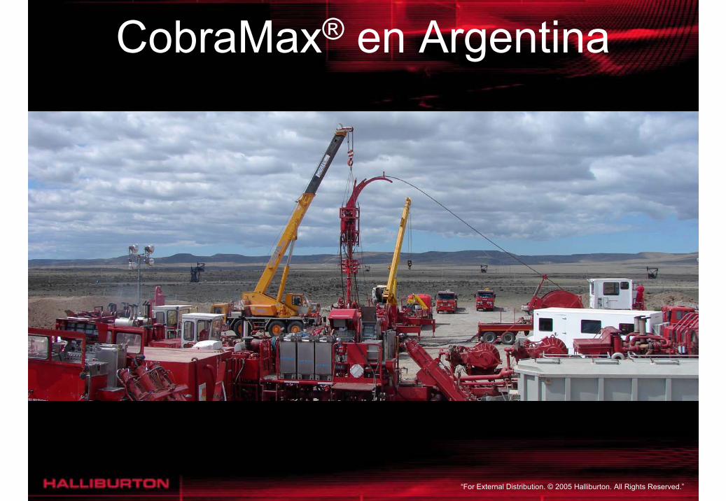
CobraMax® en Argentina

“For External Distribution. © 2005 Halliburton. All Rights Reserved.”
10/17/200616:00 16:10 16:20 16:30 16:40 16:50
10/17/200617:00
Time
0
1000
2000
3000
4000
5000
6000
7000
8000
9000
10000A
0
2
4
6
8
10
12
14
16
18
20B
0
2
4
6
8
10
12
14
16
18
20C
CT Pressure (psi) Annulus Pressure (psi) CT Rate (bpm)Annulus Pressure(bpm) Slurry Proppant Conc (lb/gal) Bottomhole Proppant Conc (lb/gal)
A A BB C C
Corte de casing
Fractura Hidráulica
Pan American Energy DeltaFrac 200 PO-960 (4) - 2088.5 m 210 sks Arena 20/40
HA LLIB UR TO NTG Version G3.2.225-Oct-06 19:35
Registro - CobraMax®
2100 m

“For External Distribution. © 2005 Halliburton. All Rights Reserved.”
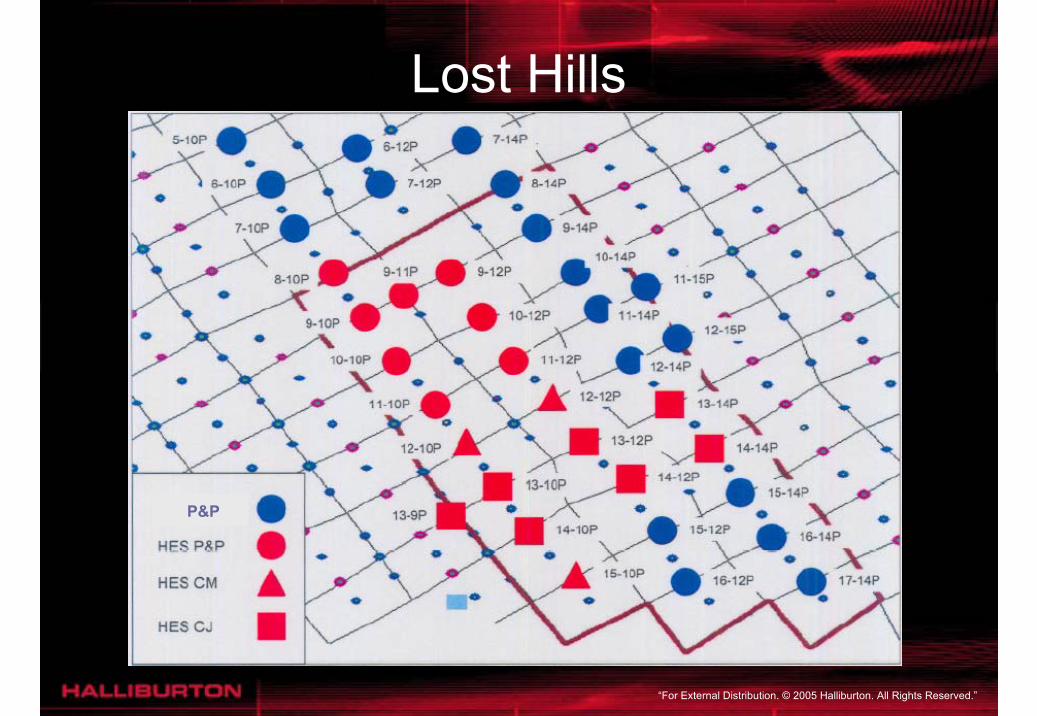
Lost Hills
• Se evaluaron 36 pozos bajo tres metodologías y doscompañías de servicios:– Punzado y Tapones (P&P)– CobraJet Frac– Cobra Max
• Criterios de evaluación fueron:– Seguridad– Performance a largo plazo (6 meses) (Costo Total por
bbl de producción)
“For External Distribution. © 2005 Halliburton. All Rights Reserved.”
Lost Hills
P&P

“For External Distribution. © 2005 Halliburton. All Rights Reserved.”
Lost Hills
Competitor P&P
18 Wells18 Wells
7 Wells
3 Wells
8 Wells
37.6%26.2%

“For External Distribution. © 2005 Halliburton. All Rights Reserved.”
Por que aplicar CobraMax®
• Múltiples fracturas en 24 horas
• Mayor selectividad de los intervalos a fracturar
• Optimización de los diseños de fracturas
• Mayor conductividad (Screen Out)
• Bajo retorno de arena
• Permite trabajar en pozos vivos

“For External Distribution. © 2005 Halliburton. All Rights Reserved.”
FIN
PREGUNTAS?
![]NIHON...M A S E S P A C 10 D SI P 0 N i B L E Francisco Calder6n Calarerni, y Jo& Pestana.Lariauri y par parte del no- qu- n!nqn 0fro fPf,,(4,-rvdor dc. !Qual tc,.- c o vio. Jos seflores](https://img.pdfslide.us/doc/110x75/5f82de8f57b410002b081887/nihon-m-a-s-e-s-p-a-c-10-d-si-p-0-n-i-b-l-e-francisco-calder6n-calarerni-y.jpg)


![ˆ˜ . ˆ#$ ˆ. ˆ ˘ &ˆ. - OSA : NYSED · 1/28/2011 · i, . У ' (1–50). txhkxth wqthf nqn havflksne nm uvkjqtlkssa[ hfvnfsxth, ptxtvtk sfnqy]^nr tgvfmtr mfhkv^fkx. /qe txhkxf](https://img.pdfslide.us/doc/110x75/5f7f5cb0229caa68a0016455/oe-osa-nysed-1282011-i-1a50-txhkxth.jpg)