Embed Size (px)
Citation preview
Expected Vibration Performance of Wood Floors AsAffected by MSR vs. VSR Lumber E-Distribution
by
Ann C. Wilson
Project submitted to the Faculty of the
Virginia Polytechnic Institute and State University
in partial fulfillment of the requirements for the degree of
MASTER OF ENGINEERING
in
Biological Systems Engineering
APPROVED:
_____________________________________ __________________________________Frank E. Woeste, Chairman J. Dan Dolan
_____________________________________ ___________________________________John V. Perumpral John V. Perumpral
May 4, 1998
Blacksburg, VA
Keywords: vibrational performance of wood floors, machine stress rated lumber, visually stress
rated lumber, modulus of elasticity
Expected Vibration Performance of Wood Floors AsAffected by MSR vs. VSR Lumber E-Distribution
by
Ann C. Wilson
Frank E. Woeste, Chairman
Biological Systems Engineering
(ABSTRACT)
A simulation study was done to investigate the effect of the coeffiecient of variation of the
modulus of elasticity (ΩE) on the vibrational performance of joist floor systems. Eight floor cases
were studied and two types of lumber were considered: MSR and VSR lumber where ΩE is 0.11
and 0.25, respectively. The expected floor vibrational performance of MSR versus VSR lumber
floors was evaluated by: 1) the probability that the fundamental frequency is less than 10 Hz and
2) the ratio of the first percentile of predicted fundamental frequency of MSR to VSR lumber.

Acknowledgements iii
Acknowledgements
My sincere thanks go to the members of my graduate committee. I am grateful to Dr. Dolan and
to Dr. Perumpral for serving on my committee. Special thanks go to Dr. Woeste for his guidance,
support and encouragement throughout my graduate studies.
My thanks also go to my fellow graduate students for their encouragement, support, and help
throughout graduate school. Their friendship and company will be missed after I leave
Blacksburg.
I would like to thank my friends and family for their love and support during my years at Virginia
Tech.
Lastly, my utmost thanks go to my Heavenly Father and my Lord Jesus Christ for being my
source of strength and blessing me with the abilities to accomplish what I have thus far.
Table of Contents iv
Table of Contents
Acknowledgements.................................................................................................................. iii
Table of Contents .................................................................................................................... iv
List of Figures........................................................................................................................... v
List of Tables ......................................................................................................................... viii
Introduction.............................................................................................................................. 1Objective ...........................................................................................................................................................2
Literature Review..................................................................................................................... 5
Procedure.................................................................................................................................14Case 1..............................................................................................................................................................14Case 2..............................................................................................................................................................16Case 3..............................................................................................................................................................17Case 4..............................................................................................................................................................18Case 5 to Case 8 ..............................................................................................................................................18
Results and Discussion ............................................................................................................20Case 1..............................................................................................................................................................20Case 2..............................................................................................................................................................25Case 3..............................................................................................................................................................33Case 4..............................................................................................................................................................38Case 5 (Load Sharing) .....................................................................................................................................45Case 6 (Load Sharing) .....................................................................................................................................51Case 7 (Load Sharing) .....................................................................................................................................58Case 8 (Load Sharing) .....................................................................................................................................63
Summary .................................................................................................................................71
Conclusions and Recommendations .......................................................................................76
References................................................................................................................................77
Vita ..........................................................................................................................................79
List of Figures v
List of Figures
Figure 1 Modulus of elasticity (E) distribution for VSR lumber (E coefficient ofvariation=0.25) floor for Case 1..........................................................................21
Figure 2 Modulus of elasticity (E) distribution for MSR lumber (E coefficient ofvariation=0.11) floor for Case 1..........................................................................22
Figure 3 Case 1 joist frequency distribution for VSR lumber floor. ...................................23
Figure 4 Case 1 joist frequency distribution for MSR lumber floor....................................24
Figure 5 Case 2 girder effective modulus of elasticity (E) distribution for VSR lumber floor ..........................................................................................................................26
Figure 6 Case 2 girder effective modulus of elasticity (E) distribution for MSR lumber floor..........................................................................................................................27
Figure 7 Case 2 girder frequency distribution for VSR lumber floor..................................29
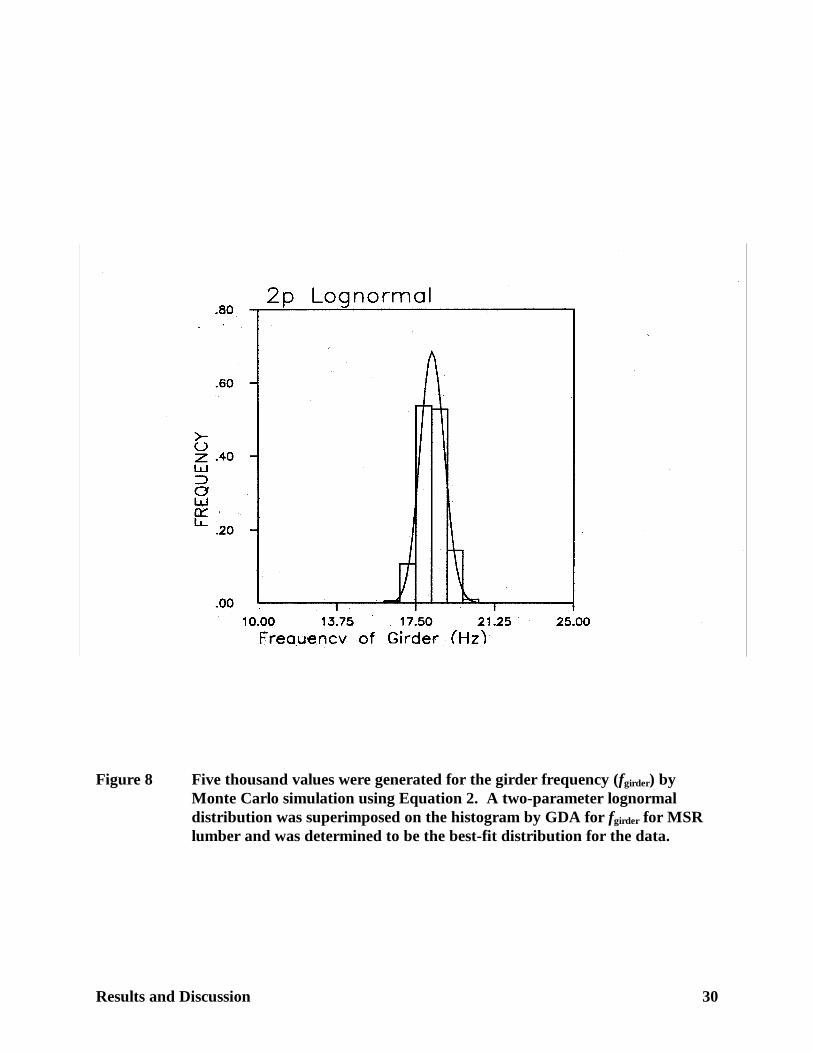
Figure 8 Case 2 girder frequency distribution for MSR lumber floor .................................30
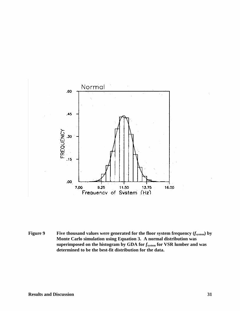
Figure 9 Case 2 floor system frequency distribution for VSR lumber floor ........................31
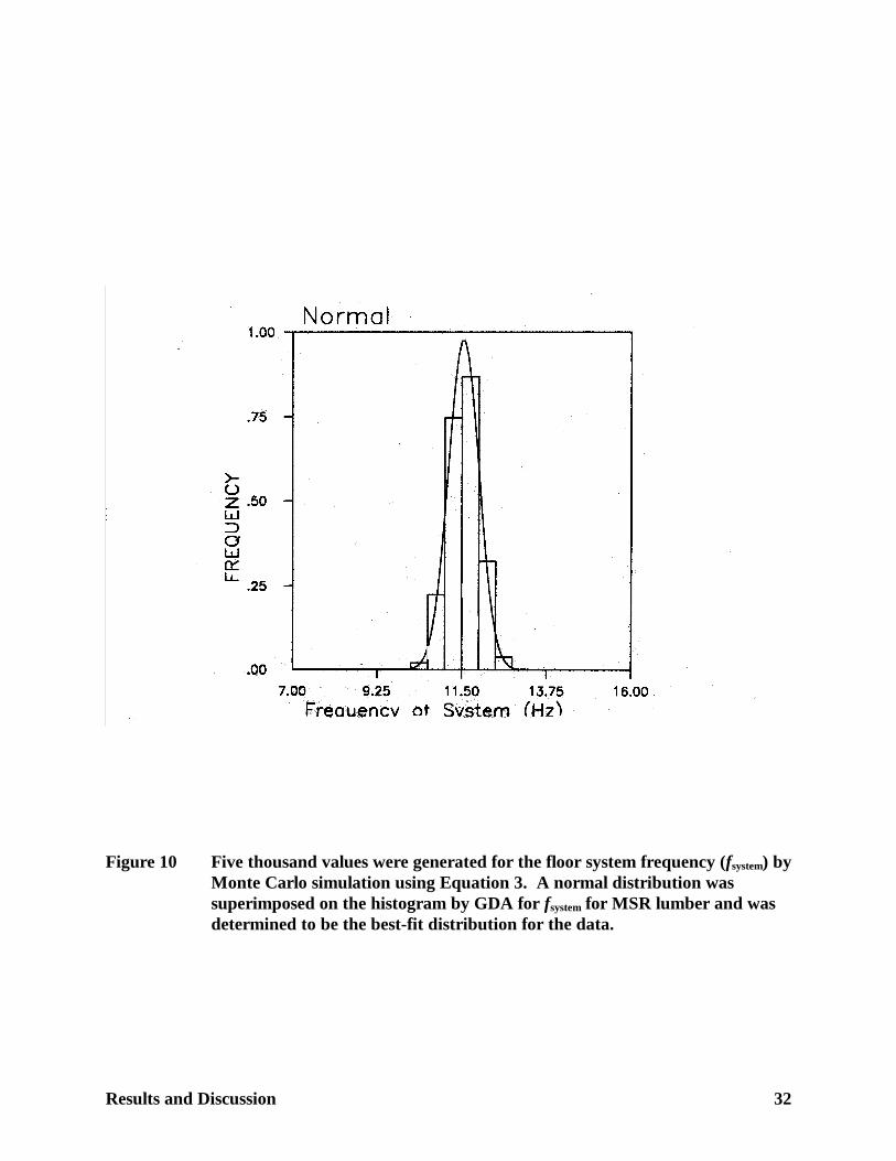
Figure 10 Case 2 floor system frequency distribution for MSR lumber floor........................32
Figure 11 Modulus of elasticity (E) distribution for VSR lumber (E coefficient of variation =0.25) floor for Case 3 .........................................................................................34
Figure 12 Modulus of elasticity (E) distribution for MSR lumber (E coefficient of variation =0.11) floor for Case 3. ........................................................................................35
Figure 13 Case 3 joist frequency distribution for VSR lumber floor ....................................36
Figure 14 Case 3 joist frequency distribution for MSR lumber floor....................................37
Figure 15 Case 4 girder effective modulus of elasticity (E) distribution for VSR lumber floor..........................................................................................................................39
List of Figures vi
Figure 16 Case 4 girder effective modulus of elasticity (E) distribution for MSR lumber floor..........................................................................................................................40
Figure 17 Case 4 girder frequency distribution for VSR lumber floor..................................41
Figure 18 Case 4 girder frequency distribution for MSR lumber floor .................................42
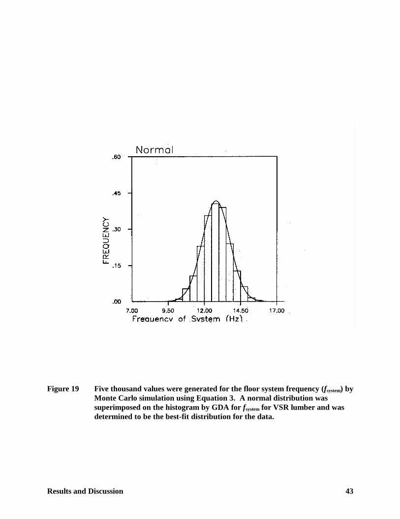
Figure 19 Case 4 floor system frequency distribution for VSR lumber floor ........................43
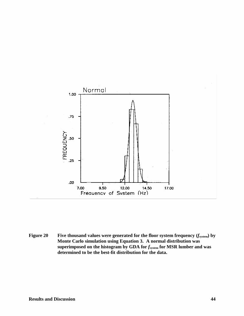
Figure 20 Case 4 floor system frequency distribution for MSR lumber floor........................44
Figure 21 Case 5 effective joist modulus of elasticity (E) distribution for VSR lumber floor ..........................................................................................................................46
Figure 22 Case 5 effective joist modulus of elasticity (E) distribution for MSR lumber floor..........................................................................................................................47
Figure 23 Case 5 joist frequency distribution for VSR lumber floor ....................................49
Figure 24 Case 5 joist frequency distribution for MSR lumber floor....................................50
Figure 25 Case 6 girder effective modulus of elasticity (E) distribution for VSR lumber floor..........................................................................................................................52
Figure 26 Case 6 girder effective modulus of elasticity (E) distribution for MSR lumber floor..........................................................................................................................53
Figure 27 Case 6 girder frequency distribution for VSR lumber floor..................................54
Figure 28 Case 6 girder frequency distribution for MSR lumber floor .................................55
Figure 29 Case 6 floor system frequency distribution for VSR lumber floor ........................56
Figure 30 Case 6 floor system frequency distribution for MSR lumber floor........................57
Figure 31 Case 7 effective joist modulus of elasticity (E) distribution for VSR lumber floor .............................................................................................................................59
Figure 32 Case 7 effective joist modulus of elasticity (E) distribution for MSR lumber floor..........................................................................................................................60
Figure 33 Case 7 joist frequency distribution for VSR lumber floor ....................................61
Figure 34 Case 7 joist frequency distribution for MSR lumber floor....................................62
List of Figures vii
Figure 35 Case 8 girder effective modulus of elasticity (E) distribution for VSR lumber floor..........................................................................................................................64
Figure 36 Case 8 girder effective modulus of elasticity (E) distribution for MSR lumber floor ..........................................................................................................................65
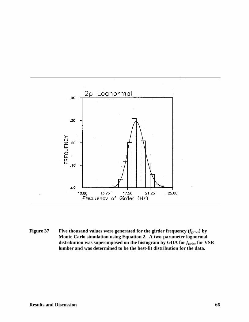
Figure 37 Case 8 girder frequency distribution for VSR lumber floor..................................66
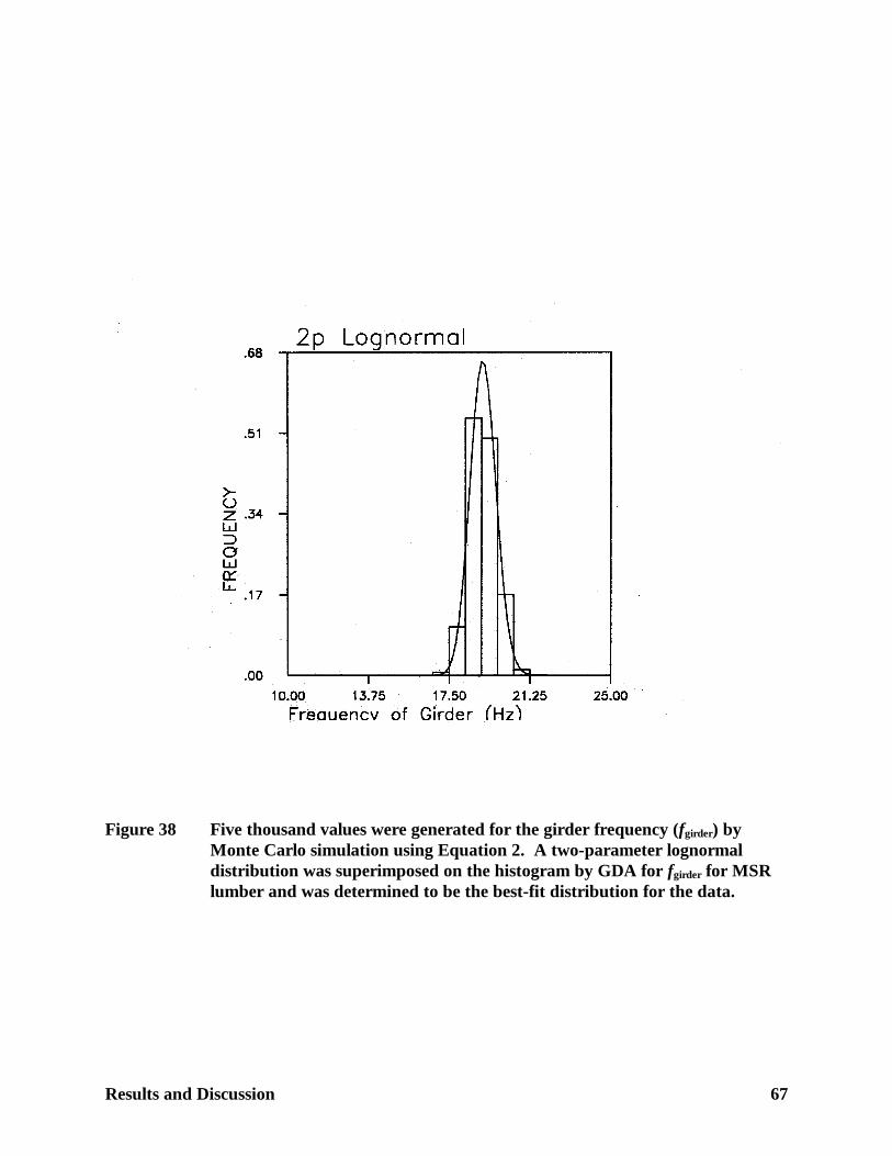
Figure 38 Case 8 girder frequency distribution for MSR lumber floor .................................67
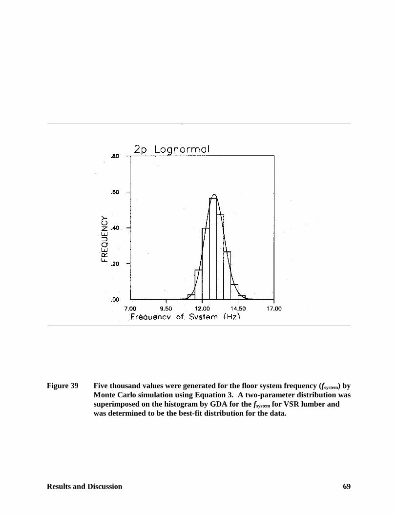
Figure 39 Case 8 floor system frequency distribution for VSR lumber floor. .......................69
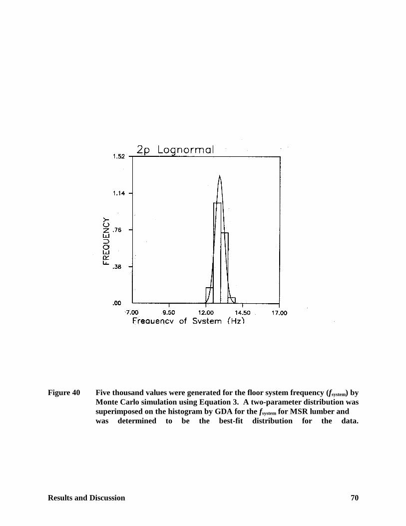
Figure 40 Case 8 floor system frequency distribution for MSR lumber floor........................70
List of Tables viii
List of Tables
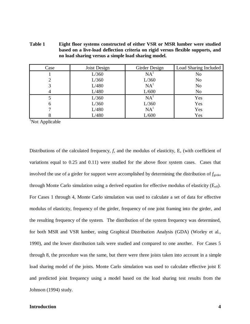
Table 1 Summary of the eight floor cases that were constructed of either VSR or MSRlumber. ................................................................................................................ 4
Table 2 Summary of the measures of expected vibrational performance of floor case 1 andfloor case 2.........................................................................................................72
Table 3 Summary of the measures of expected vibrational performance of floor case 3 andfloor case 3.........................................................................................................73
Table 4 Summary of the measures of expected vibrational performance of floor case 5 andfloor case 6.........................................................................................................74
Table 5 Summary of the measures of expected vibrational performance of floor case 7 andfloor case 8.........................................................................................................75
Introduction 1
Introduction
Traditionally, most wood floors were constructed with solid-sawn lumber joists and designed
according to the L/360 live-load deflection limit. This deflection criterion was developed to
prevent cracks in the ceiling plaster, and probably not to limit vibrations (Percival, 1979).
Vibrational performance of floor systems was not a major issue in previous decades because the
floor spans were relatively short. However, recent architectural changes have created a demand
for longer spans in floor systems. As a result, engineered-wood products such as I-joists and
parallel-chord trusses were developed to satisfy this demand for longer spans. These engineered-
wood products offer high strength-to-weight and high stiffness-to-weight ratios (Kalkert, 1995).
Unfortunately, the switch to longer span floors have decreased the serviceability of floors with
regard to annoying vibrations. Most people are sensitive to vibrations in the 8 to 10 Hz range
because some human organs have a natural frequency of about 4 to 8 Hz. Therefore, when a
floor is vibrating at the same range in frequency, it is perceived as uncomfortable. The
unacceptable vibrational performance of some long span wood floors reveal that the L/360 live-
load deflection criterion is not alone sufficient in designing a wood floor for 100 percent
acceptable vibrational performance.
Currently, U.S. codes do not contain design criterion for controlling floor vibrations. Much
research has been conducted on the subject of floor vibrations and several design criteria have
been proposed to allow designers to check for acceptable vibrational performance of floors.
Introduction 2
However, none are widely accepted due to the complexity of some criteria and the lack of readily
available information for the designer (Dolan, 1994). Research conducted by Johnson (1994) at
Virginia Tech have resulted in the development of a design criterion that will eliminate most
unacceptable and marginally acceptable floor systems (floor systems in or close to the 8 to 10 Hz
range) and will aid designers in designing acceptable floors with acceptable vibration performance.
Solid-sawn lumber have different grading systems. Two such grading systems are visually stress
rated lumber (VSR) and machine stress rated lumber (MSR). Due to the differences in grading,
MSR and VSR lumber have differences in the coefficient of variation of modulus of elasticity
(ΩE). VSR lumber has an ΩE of 0.25 and MSR lumber has an ΩE of 0.11 (AF&PA, 1997). This
difference in E-variability between MSR and VSR lumber affects the strength and serviceability
performance of the structure. Variability of the modulus of elasticity between MSR and VSR
lumber is recognized in strength design and addressed in the NDS (buckling capacity of members
under compression stress, truss compression chords, and beam stability). Basically, the lower the
ΩE, the higher the capacity of the member with respect to stability issues because the likelihood of
a very low E-value is lessened. However, the variability of modulus of elasticity is not addressed
in the NDS with regards to serviceability (i.e. deflection and vibrations performance), instead the
published average values of modulus of elasticity are used in serviceability calculations.
Objective
The objective of this simulation project was to investigate the effect of the coefficient of variation
of the modulus of elasticity (ΩE) of lumber on the vibration performance of joist floor systems.
Introduction 3
Two types of lumber will be considered: machine stress rated lumber (MSR) and visually stress
rated lumber (VSR) where the assumed ΩE’s are 0.11 and 0.25, respectively. Expected floor
vibrational performance of MSR lumber versus VSR lumber will be evaluated by 1) the
probability that the fundamental frequency is less than 10 Hz, and 2) a comparative measure of
the ratio of the first percentile of the distribution for fundamental frequency of vibration, f, of
MSR lumber to the first percentile of the distribution for f of VSR lumber:
VSR
MSR
f
f
01.0
01.0 (1)
Two floor systems will be considered: 1) joists supported on both ends by concrete blocks (rigid
supports) and 2) joists supported by a simple span girder (flexible support) on one end and by
concrete blocks on the other end.
This study involved a total of eight cases that are summarized by Table 1. Case 1 involved a floor
system of joists supported by rigid supports with the span of the joists designed to the L/360 live-
load deflection limit. Case 2 involved a floor system with joists supported by a simple span girder
on one end and concrete blocks on the other end. The span of both the girder and joists were
designed to the L/360 live-load deflection limit. Case 3 had the same floor system as Case 1, but
the joist span was designed to the L/480 live-load deflection limit. The floor system for Case 4
was the same as Case 2, but the joist span was designed to L/480 while the girder span was
designed to L/600. Cases 5 through 8 were a repeat of Cases 1 through 4 using an effective joist
E based on a load sharing model.
Introduction 4
Table 1 Eight floor systems constructed of either VSR or MSR lumber were studiedbased on a live-load deflection criteria on rigid versus flexible supports, andno load sharing versus a simple load sharing model.
Case Joist Design Girder Design Load Sharing Included1234
L/360L/360L/480L/480
NA1
L/360NA1
L/600
NoNoNoNo
5678
L/360L/360L/480L/480
NA1
L/360NA1
L/600
YesYesYesYes
1Not Applicable
Distributions of the calculated frequency, f, and the modulus of elasticity, E, (with coefficient of
variations equal to 0.25 and 0.11) were studied for the above floor system cases. Cases that
involved the use of a girder for support were accomplished by determining the distribution of fgirder
through Monte Carlo simulation using a derived equation for effective modulus of elasticity (Eeff).
For Cases 1 through 4, Monte Carlo simulation was used to calculate a set of data for effective
modulus of elasticity, frequency of the girder, frequency of one joist framing into the girder, and
the resulting frequency of the system. The distribution of the system frequency was determined,
for both MSR and VSR lumber, using Graphical Distribution Analysis (GDA) (Worley et al.,
1990), and the lower distribution tails were studied and compared to one another. For Cases 5
through 8, the procedure was the same, but there were three joists taken into account in a simple
load sharing model of the joists. Monte Carlo simulation was used to calculate effective joist E
and predicted joist frequency using a model based on the load sharing test results from the
Johnson (1994) study.
Literature Review 5
Literature Review
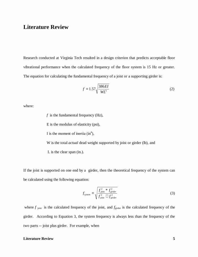
Research conducted at Virginia Tech resulted in a design criterion that predicts acceptable floor
vibrational performance when the calculated frequency of the floor system is 15 Hz or greater.
The equation for calculating the fundamental frequency of a joist or a supporting girder is:
3
386571
WL
EI.f = (2)
where:
f is the fundamental frequency (Hz),
E is the modulus of elasticity (psi),
I is the moment of inertia (in4),
W is the total actual dead weight supported by joist or girder (lb), and
L is the clear span (in.).
If the joist is supported on one end by a girder, then the theoretical frequency of the system can
be calculated using the following equation:
22
22
girderjoist
girderjoistsystem
ff
f*ff
+= (3)
where f joist is the calculated frequency of the joist, and fgirder is the calculated frequency of the
girder. According to Equation 3, the system frequency is always less than the frequency of the
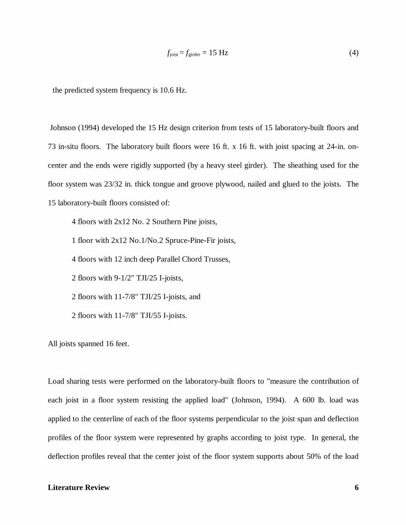
two parts -- joist plus girder. For example, when
Literature Review 6
fjoist = fgirder = 15 Hz (4)
the predicted system frequency is 10.6 Hz.
Johnson (1994) developed the 15 Hz design criterion from tests of 15 laboratory-built floors and
73 in-situ floors. The laboratory built floors were 16 ft. x 16 ft. with joist spacing at 24-in. on-
center and the ends were rigidly supported (by a heavy steel girder). The sheathing used for the
floor system was 23/32 in. thick tongue and groove plywood, nailed and glued to the joists. The
15 laboratory-built floors consisted of:
4 floors with 2x12 No. 2 Southern Pine joists,
1 floor with 2x12 No.1/No.2 Spruce-Pine-Fir joists,
4 floors with 12 inch deep Parallel Chord Trusses,
2 floors with 9-1/2" TJI/25 I-joists,
2 floors with 11-7/8" TJI/25 I-joists, and
2 floors with 11-7/8" TJI/55 I-joists.
All joists spanned 16 feet.
Load sharing tests were performed on the laboratory-built floors to "measure the contribution of
each joist in a floor system resisting the applied load" (Johnson, 1994). A 600 lb. load was
applied to the centerline of each of the floor systems perpendicular to the joist span and deflection
profiles of the floor system were represented by graphs according to joist type. In general, the
deflection profiles reveal that the center joist of the floor system supports about 50% of the load
Literature Review 7
while the neighboring joists carry approximately the other 50% (25% each to the two adjacent
joists). From this observation, the “apparent stiffness” of the loaded joist in the center of the floor
is twice as much as the stiffness predicted by standard deflection formula and the tabulated E for
the lumber grade. The center joist of each deflection profile had different deflections (relative to
neighboring joists) depending on the joist type. The average deflection of the center joist of both
2x12 No.2 Southern Pine and 2x12 No.1/No.2 Spruce-Pine-Fir solid sawn lumber was 0.15
inches. The average deflection of the center joist of the 12-inch deep parallel chord trusses was
0.16 inches. For I-joists, the deflections for 9-1/2" TJI/25, 11-7/8" TJI/25, and 11-7/8" TJI/55
were 0.19 inches, 0.12 inches, and 0.09 inches, respectively. A conclusion that can be drawn
from these deflection profiles is the depth and the type of joist used will affect how much the
loaded joist deflects relative to the neighboring joists.
Johnson (1994) tested 73 in-situ floors at various construction sites near Blacksburg, Virginia.
The 73 in-situ floors consisted of:
46 floors with 2x10 solid-sawn joists spanning 7 to 23 feet,
4 floors with 2x12 solid-sawn joists spanning 14.5 to 16 feet,
3 floors with 18" deep parallel chord trusses spanning 9 to 25 feet,
13 floors with 20" deep parallel chord trusses spanning 25 to 28 feet,
2 floors with 24" deep parallel chord trusses spanning 30 feet,
2 floors with 11 1/4" deep I-joist floors spanning 20 feet, and
3 floors with 16" deep I-joist spanning 14 to 20 feet.
Literature Review 8
The joist spacing ranged from 12 to 24 in. on center, with the majority spaced at 16 in. on center.
Some of these floors were bare while others were part of nearly completed structures.
The predicted fundamental frequency for the 86 floors was calculated using Equations 2 and 3.
Heel drop tests were used to measure the frequency of each floor system, and the vibration
performance of each floor system was subjectively rated as acceptable, marginal, or
unacceptable (Johnson, 1994). Measured frequencies compared favorably with the predicted
frequencies using Equation 2 which validated the equations used for calculating the frequency of
the individual joist.
It was determined from the measured data that a frequency of 15 Hz, using Equation 2, provides
the distinction between unacceptable and acceptable floors for all floors evaluated. Johnson
(1994) concluded that the frequency of the floor should be calculated based upon only the self
weight of the floor since the proposed design criterion was based on tests of bare floors. If the
calculated frequency is greater than 15 Hz, then the vibration performance of the floor is expected
to be acceptable.
Shue's (1995) study provided further validation of the Johnson study. The difference between the
two studies was that Shue tested occupied floors as well as unoccupied floors. The Shue study
took into account the effect of partitions or the overall structure itself on the vibration
performance of the floor system. Shue tested 106 in-situ wood floors of which 20 were originally
in the Johnson study. The result of this study validated the design criterion proposed by the
Johnson study for unoccupied floors. However, for occupied floors, Shue concluded that the
Literature Review 9
frequency of the floor system must be greater than 14 Hz in order for it to be considered
acceptable.
McGuire (1997) proposed a design rule of thumb that is based on dead load deflection. He used
Equation 2 from above and the deflection equation for a simple span joist with uniform dead load
in developing this design rule. His proposed vibration design rule causes the fundamental
frequency to be greater than 15 Hz when the calculated dead load deflection is less than 0.055
inches. Actual dead load and not the design dead load is to be used in calculating the deflection
of the joist. The reader is referred to the article for the mathematics in developing this rule of
thumb.
Dolan and Skaggs (1994) stated that one of the main goals in the Johnson study (1994) in
developing the criterion was to eliminate the majority of complaints about annoying floor
vibrations. The criterion was set at 15 Hz which eliminated the floors judged to be unacceptable
and marginally acceptable as well as a few judged to be acceptable. A result of this criteria is the
decrease in allowable span for parallel-chord trusses in long-span floors. Dolan and Skaggs stated
that the maximum span to depth ratio (l/d) is reduced by 50 percent as the span increases from 10
to 30 feet for parallel-chord trusses spaced at 24 inches on center, with chord modulus of
elasticities of 1.6 and 1.9 million psi and sheathed with 23/32” plywood. Dolan and Skaggs also
compared the criteria with the L/360 live-load deflection criteria using the parallel-chord truss
floor system described above with chord modulus of elasticity of 1.9 million psi. For spans
between 22 and 30 feet, the vibration criteria falls between the L/360 and L/480 live-load
Literature Review 10
deflection criteria. The L/360 live-load deflection criteria is sufficient for spans up to 22 feet but
after 22 feet the vibration criteria developed by Johnson should be used.
Dolan et al. (1995) studied the effect of imposed load on floor vibrations. Solid-sawn wood joist
floors were studied. There were four 16 ft. by 16 ft. laboratory-built floors designed to the L/360
live-load deflection limit and a live load of 40 psf. The joist size was 2x12 Southern Pine solid-
sawn joists spaced at 24 inches on center with 23/32 inch tongue and groove plywood nailed and
glued to the joists. There were two levels of ΩE for the joists: 9 percent and 28 percent. Three
levels of live load (0 psf, 15 psf, and 40 psf) by means of bags of steel pellets were imposed on the
floor system and the dynamic response of the solid-sawn wood joist floors was examined by
looking at 3 parameters: natural frequency, damping ratios, and RMS acceleration. The natural
frequency of the joist floors decreased as the imposed load increased. No conclusions could be
drawn for damping ratio since the results were inconsistent. The frequency weighted RMS
acceleration for a joist floor decreased as the imposed load increased. This result was explained
by the principle of conservation of momentum – the heavier the floor the more difficult it is to set
it into motion compared to a lighter floor. The final conclusion from this study was that ΩE had
little or no effect on the measured vibration responses of the floors tested.
Kalkert et al. (1995) evaluated six design criteria for floor vibrations. Deflection factors (from
Span/Deflection Factor) were determined for each criteria. The values for these deflection factors
were two to four times larger than the deflection factor of 360 (L/360). The deflection factors
ranged from 701 to 1448. The deflection factor of 701 was determined from the Canadian Wood
Council (CWC) criterion. The deflection factors calculated excluded the stiffening effects of
Literature Review 11
sheathing. The authors stated that if sheathing were included in the calculations the values for the
deflection factors would be lower. Six different floor types (solid-sawn, I-joists, etc.) were then
evaluated for acceptable vibrational performance by each criteria. It was found that a floor
system would need to be designed to a minimum L/701 live-load deflection limit in order for the
predicted vibrational performance of the floor to be acceptable. A consequence of designing to
this stricter deflection limit from the traditional L/360 limit is a 20 percent reduction in span. The
authors concluded that further research is needed in determining an appropriate deflection limit
based on experimental investigations and economic analysis.
Chui (1994) offered suggestions for optimizing the vibrational performance of wood floor systems
and retrofitting. A number of variables can affect the vibrational performance of floors. Some of
these variables are joist size and spacing, between-joist bridging, composite action between joists
and flooring, flooring panel thickness and ceiling boards, and mass distribution. When designing
floor systems, Chui suggested selecting a heavier floor. A heavy floor will reduce the amplitude
of the vibration. Basically, having a floor vibrate at low amplitudes, high frequency and high
damping is not as annoying as a floor vibrating at high amplitudes, low frequency and low
damping. Therefore, a heavy floor mass is beneficial because it lowers the amplitude. However,
he states that the heavier floor will also reduce the frequency but the reduction is small. An
example of a heavier floor design would be to use low-grade joists with large cross-section and
narrow joist spacing. Between-joist bridging was also suggested because wood floors are highly
orthotropic – the stiffness along the span of the joist is higher than the stiffness across joists.
Between-joist bridging increases the capacity of the floor system to share loads across joists. In
addition to using between-joist bridging, a continuous bottom strap was suggested to provide
Literature Review 12
continuity on the bottom side of the bridging system. Chui also suggested using rigid glue in
addition to nailing to increase the degree of composite action between solid-sawn joists and the
flooring. However, Chui added that the improvement in the vibrational performance of floors
built with engineered wood products is not significant. Oriented strand board (OSB) was
suggested over plywood for floor sheathing due to its higher density which produces a lower
vibrational amplitude. Finally, with the exception of very wide floors, Chui suggested an
unbalanced, imposed mass distribution on floors. The above recommendations were also offered
as suggestions in retrofitting existing floors.
Fridley and Rosowsky (1994) addressed and summarized the service-load behavior of wood floor
systems as follows. Load distribution and smoothing of the deflection profile are two actions that
take place with two-way action. For load distribution in a floor system, the load carried by each
joist is proportional to its stiffness. As a result of load distribution, the deflection of the joists in
the floor system is affected. There is a smoothing of the deflection profile which is similar to that
of a real floor. Assuming full composite action, a sheathed floor would have less deflection than a
bare floor. A composite floor with load sharing has a similar deflection profile to that of a real
floor. Gaps in the sheathing can affect two-way and composite action. However, staggering the
sheathing lessens this negative affect on two-way action. For composite action under uniform
load, they concluded that it is acceptable to not account for gaps and assume full composite action
when computing the deflection.
Rosowsky and Fridley (1994) also added that creep in floor systems is significantly less than creep
in single members. Fridley and Rosowsky suggested using a system factor for serviceability to
address the effects of the behavior of the floor system, versus a single member design approach.
Literature Review 13
Suddarth et al. (1997) performed a simulation study of the influence of ΩE on floor performance.
The simulation study involved two types of floors, machine stress rated (MSR) and visually stress
rated (VSR) joists. There were two sizes for the joists, 2x8 and 2x12. The model used in the
simulation included the effect of sheathing and load sharing. The purpose of this study was to
compare the deflection performance of MSR floors against the deflection performance of VSR
floors using average deflection and soft-spot deflection as measures of performance. Soft-spot
deflection was defined as the maximum deflection of three adjacent joists in a floor system.
Simulations yielded distributions for average deflection and soft-spot deflection that were
reported in terms of L/∆ where L was the span and ∆ was the deflection. The 10th percentile of
MSR and VSR floors for average deflection and soft-spot deflection were compared to show the
difference in expected floor performance between MSR and VSR floors. The results based on
average deflection were that a 1.45x10⁶ psi MSR E-grade floor performed equivalently to a
1.6x10⁶ psi VSR E-grade floor. For soft spot deflection, a 1.4x10⁶ psi MSR E-grade floor
performed equivalently to a 1.6x10⁶ psi VSR E-grade floor.
Procedure 14
Procedure
Variables E and f in Equation 2 were the main focus in this project. Floor systems studied
consisted of eight 2x10 joists spaced at 16 in. on center. For Cases 1, 2, 5, and 6, the span of the
joists was 16'-1" and the span of the 3-ply 2x10 girder was 11'-4". For Cases 3, 4, 7, and 8, the
span of the joists was 14’-10” and the span of the 3-ply 2x10 girder was 11’-3”. The joists and
the girder were No. 2 KD19 Southern Pine. An individual joist was studied for Cases 1 through 4
instead of eight joists, and thus load sharing due to floor sheathing was not taken into account.
However, in Cases 5 through 8, three joists were studied and thus a measure of load sharing was
taken into account as described later.
In order to investigate the effect of ΩE on the expected vibrational performance of each floor
system, the frequency distributions were determined for each floor case.
Case 1
The E was assumed to be lognormally distributed (Suddarth et al., 1975). This assumption was
made because it allows us to vary the coefficient of variation easily. It is also a reasonable
selection for E because the values for E are positive and the lognormal distribution falls above
zero along the x-axis. The parameters for the E-distribution were calculated using the following
equations from Ang and Tang (1975):
Procedure 15
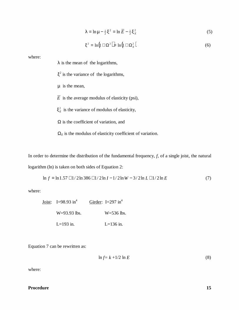
2212
21 lnln EE ξ−=ξ−µ=λ (5)
( ) ( )222 1ln1ln EΩ+=Ω+=ξ (6)
where: λ is the mean of the logarithms,
ξ2 is the variance of the logarithms,
µ is the mean,
E is the average modulus of elasticity (psi),
2Eξ is the variance of modulus of elasticity,
Ω is the coefficient of variation, and
ΩE is the modulus of elasticity coefficient of variation.
In order to determine the distribution of the fundamental frequency, f, of a single joist, the natural
logarithm (ln) is taken on both sides of Equation 2:
ELWIf ln2/1ln2/3ln2/1ln2/1386ln2/157.1lnln +−−++= (7)
where:
Joist: I=98.93 in4 Girder: I=297 in4
W=93.93 lbs. W=536 lbs.
L=193 in. L=136 in.
Equation 7 can be rewritten as:
ln f= k +1/2 ln E (8)
where:
Procedure 16
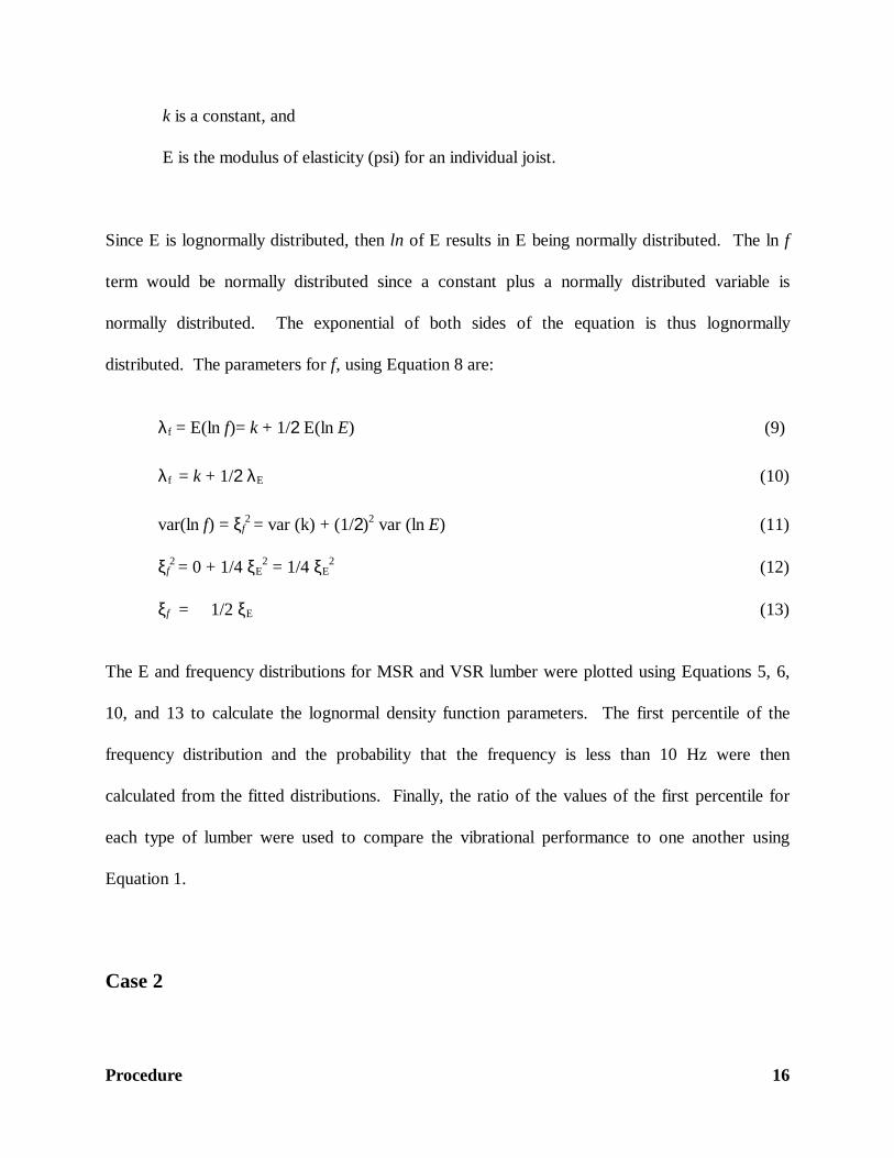
k is a constant, and
E is the modulus of elasticity (psi) for an individual joist.
Since E is lognormally distributed, then ln of E results in E being normally distributed. The ln f
term would be normally distributed since a constant plus a normally distributed variable is
normally distributed. The exponential of both sides of the equation is thus lognormally
distributed. The parameters for f, using Equation 8 are:
λf = E(ln f)= k + 1/2 E(ln E) (9)
λf = k + 1/2 λE (10)
var(ln f) = ξf2 = var (k) + (1/2)2 var (ln E) (11)
ξf2 = 0 + 1/4 ξE
2 = 1/4 ξE2 (12)
ξf = 1/2 ξE (13)
The E and frequency distributions for MSR and VSR lumber were plotted using Equations 5, 6,
10, and 13 to calculate the lognormal density function parameters. The first percentile of the
frequency distribution and the probability that the frequency is less than 10 Hz were then
calculated from the fitted distributions. Finally, the ratio of the values of the first percentile for
each type of lumber were used to compare the vibrational performance to one another using
Equation 1.
Case 2
Procedure 17
The distributions of the girder modulus of elasticity and the distribution of its frequency needed to
be determined first before determining the system frequency. The E-distribution of the girder
differs from the E-distribution of the joist since the girder has three members acting together
instead of one. If three bending members are connected such that they deflect the same amount,
then the effective E (Eeff) is:
3321 EEE
Eeff
++= (14)
In this study, it was assumed that the three plys of the girder deflect the same amount due an
assumed typical construction nailing between plies.
Using Equations 2 and 14, 5000 values were generated for Eeff and girder frequency (fgirder) using
Monte Carlo simulation. The program, GDA (Worley et al., 1990), was used to determine the
best-fit distribution for the data. Using 5000 values of joist E, Equation 2 was used to calculate
5000 values of fjoist. Lastly, 5000 values of fsystem were calculated using Equation 3. GDA was
used to determine the best fitting distribution of fsystem and then the first percentile and the
probability of the frequency being less than 10 Hz were calculated for MSR and VSR lumber.
The first percentile for both types of lumber were then used to compare the predicted vibrational
performance to one another using Equation 1.
Case 3
The procedure for case 3 was the same as the Case 1 procedure. However, the values for the
different variables in Equation 7 were different because the joist span was designed to the L/480
live-load deflection limit. The values of the variables are:
Procedure 18
Joist: I=98.93 in4 Girder: I=296.79 in4
W=86.63 lbs. W=502 lbs.
L=178 in. L=135 in.
Case 4
The procedure for Case 4 was the same as Case 2, but with differing values for the variables
because the joist and girder span were designed for the L/480 and L/600 live-load deflection
limits, respectively.
Case 5 to Case 8
Cases 1 through 4 were repeated using an effective joist E, Ej, based and justified by the load
sharing results from the Johnson study. The model used was:
Ej=0.25EL + 0.5EC +0.25ER (15)
where the E’s represent three joists in a row in a floor. EL is the left joist, EC is the center joist
impacted by a footfall, and ER is the right joist, and the three were considered independent
random variables.
However, except for the procedures in obtaining the data for E and fjoist, the procedures used for
Cases 5 through 8 were the same as Cases 1 through 4. Monte Carlo simulation was used to
generate 5000 values for each variable in Equation 15. Then, Ej was used in Equation 2 in place
of the variable E to calculate 5000 values of fjoist. GDA was used to determine the best-fit

Procedure 19
distribution for the data for Ej and fjoist. For Case 6 and Case 8 the 5000 values for fjoist and Ej
along with fgirder values were then substituted into Equation 3 to produce 5000 values for fsystem.
Results and Discussion 20
Results and Discussion
Case 1
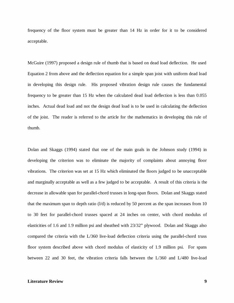
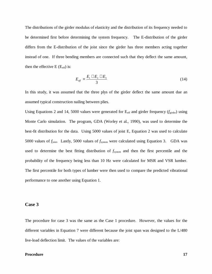
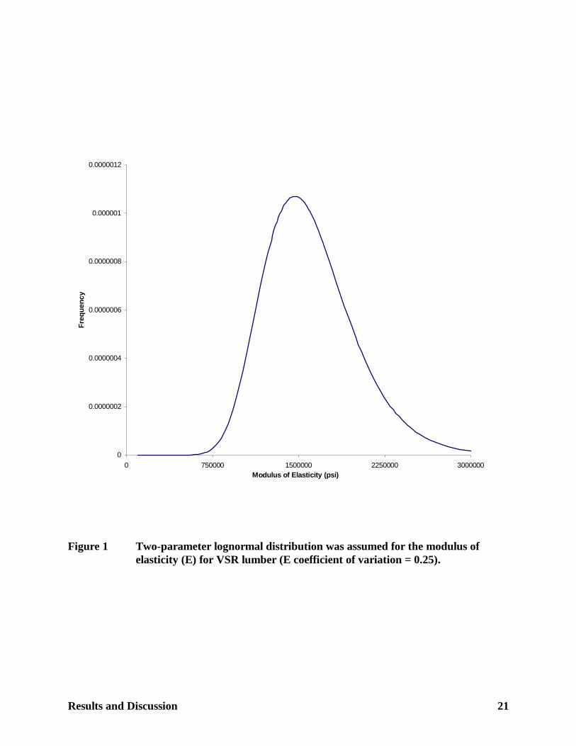
The assumed modulus of elasticity (E) distribution for VSR lumber is shown in Figure 1. The
modulus of elasticity was assumed to be lognormally distributed. It ranges from about 700,000
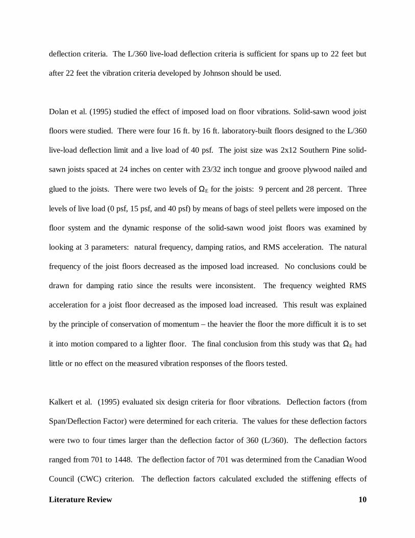
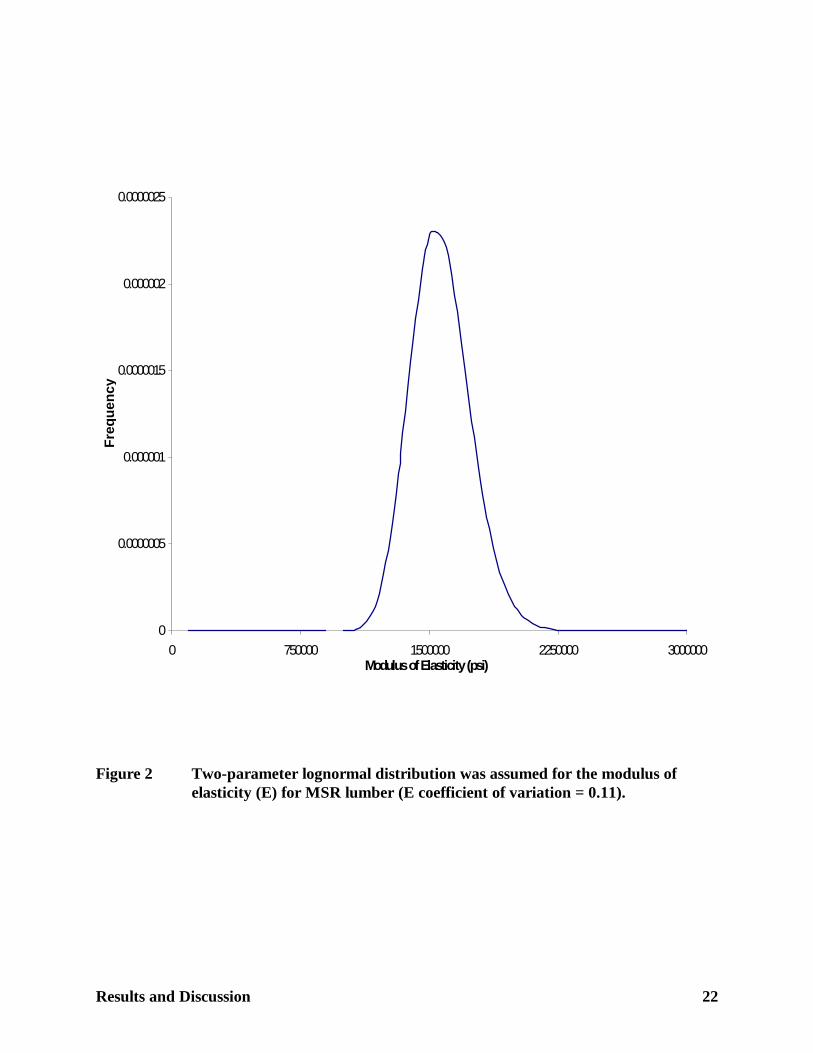
psi to 3,000,000 psi. The modulus of elasticity for MSR lumber was also assumed to be
lognormally distributed with a coefficient of variation of 0.11 and it is shown in Figure 2. It
ranges from about 1,000,000 psi to 2,250,000 psi. The E-distribution for MSR lumber is
dramatically less variable than the E-distribution for VSR lumber by inspecting Figures 1 and 2.
This lower variability of the E-distribution in Figure 2 compared to the E-distribution in Figure 1
can be attributed to MSR lumber having a lower coefficient of variation than VSR lumber.
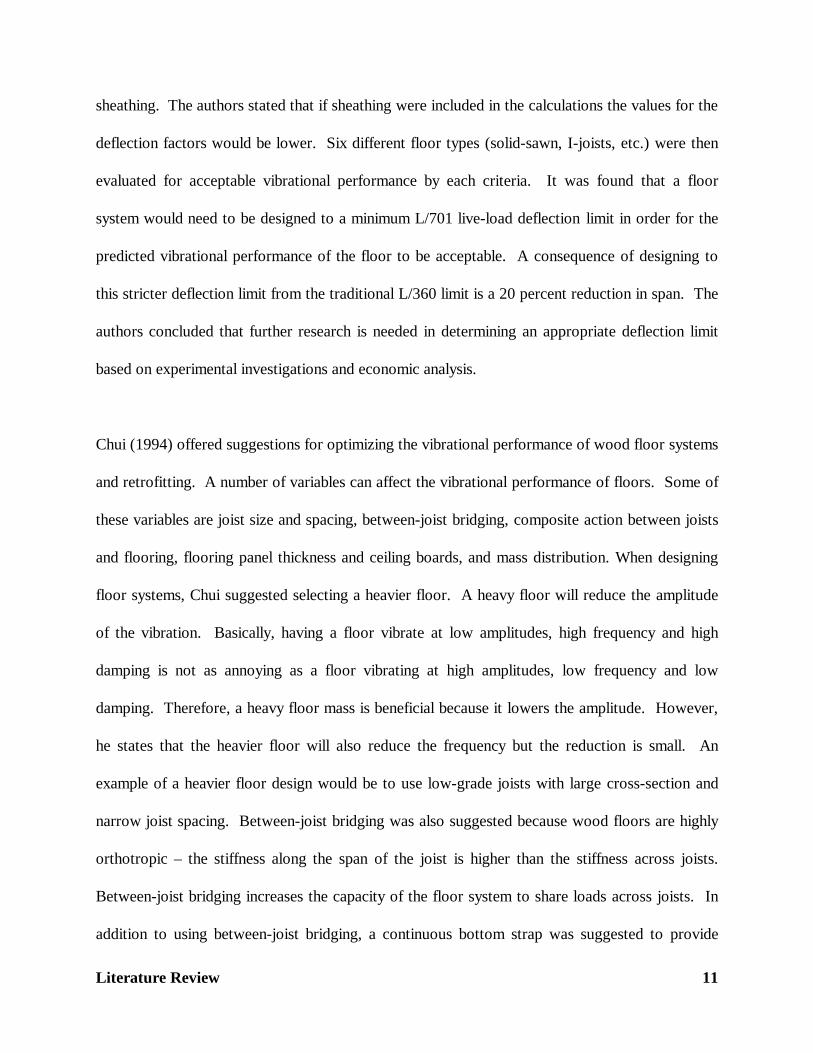
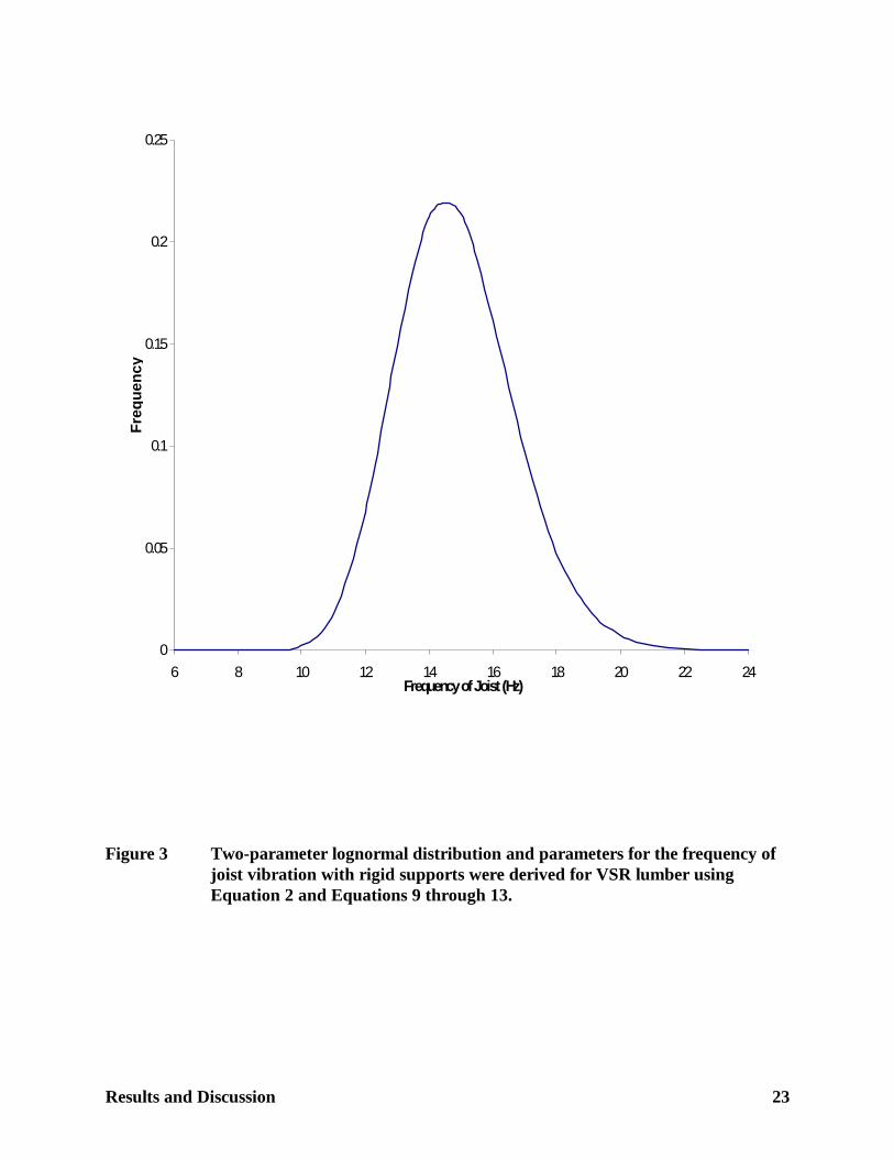
Figure 3 represents the calculated frequency distribution of a joist for VSR lumber and it is
lognormally distributed because E was assumed to be lognormal. It ranges from about 10 Hz to
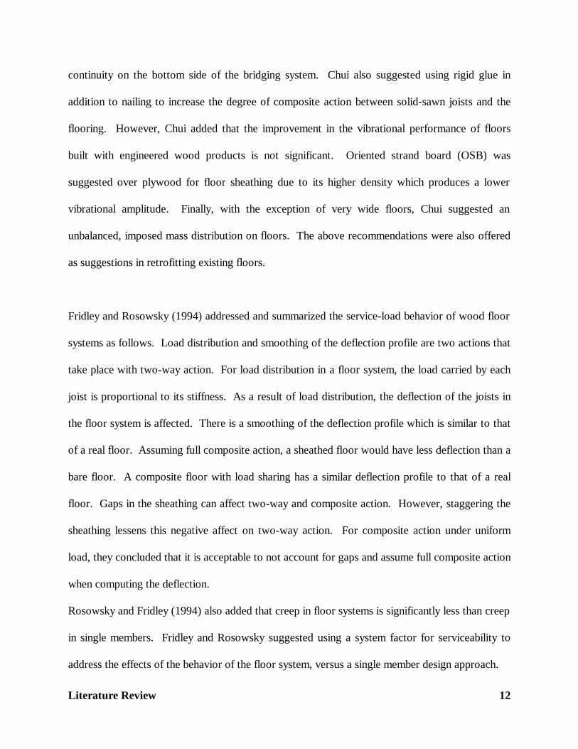
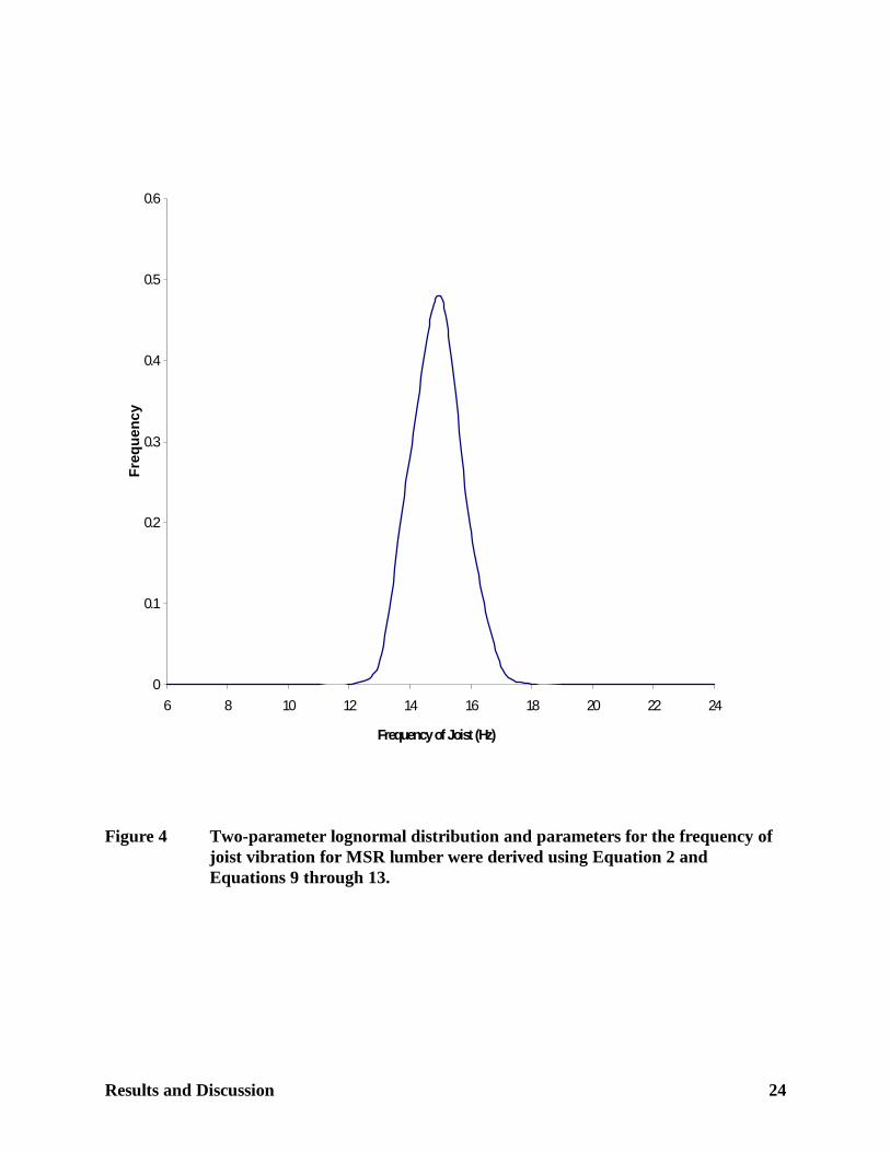
22 Hz. The calculated frequency distribution for MSR lumber is shown in Figure 4. It also is
lognormally distributed and is noticeably less variable than fjoist depicted in Figure 3.
Based on Equations 10 and 13, the E-distribution affects the predicted fundamental frequency
distribution of a joist. For example, the E for MSR lumber is less variable than VSR lumber (0.11
versus 0.25). ξ2 in Equation 6 was calculated based on ΩE. For MSR lumber, a lower ΩE would
Results and Discussion 21
Figure 1 Two-parameter lognormal distribution was assumed for the modulus of elasticity (E) for VSR lumber (E coefficient of variation = 0.25).
0
0.0000002
0.0000004
0.0000006
0.0000008
0.000001
0.0000012
0 750000 1500000 2250000 3000000 Modulus of Elasticity (psi)
Fre
quen
cy
Results and Discussion 22
Figure 2 Two-parameter lognormal distribution was assumed for the modulus of elasticity (E) for MSR lumber (E coefficient of variation = 0.11).
0
0.0000005
0.000001
0.0000015
0.000002
0.0000025
0 750000 1500000 2250000 3000000Modulus of Elasticity (psi)
Fre
que
ncy
Results and Discussion 23
Figure 3 Two-parameter lognormal distribution and parameters for the frequency of joist vibration with rigid supports were derived for VSR lumber using Equation 2 and Equations 9 through 13.
0
0.05
0.1
0.15
0.2
0.25
6 8 10 12 14 16 18 20 22 24Frequency of Joist (Hz)
Fre
que
ncy
Results and Discussion 24
Figure 4 Two-parameter lognormal distribution and parameters for the frequency of joist vibration for MSR lumber were derived using Equation 2 and Equations 9 through 13.
0
0.1
0.2
0.3
0.4
0.5
0.6
6 8 10 12 14 16 18 20 22 24
Frequency of Joist (Hz)
Fre
quen
cy
Results and Discussion 25
cause the standard deviation of the logarithms of E, ξE , to be lower. Since ξE is the standard
deviation for the lognormal density, the variability of the predicted frequency is lower (Figure 4).
The probability that the frequency will be less than 10 Hz in Figure 3 is 0.0008. The first
percentile of the distribution is 11.06 Hz. For Figure 4, the probability that the frequency will be
less than 10 Hz is approximately zero. The first percentile of the distribution for MSR is 13.09
Hz, which is about 18 percent more than the first percentile for VSR, lumber (Figure 3).
Case 2
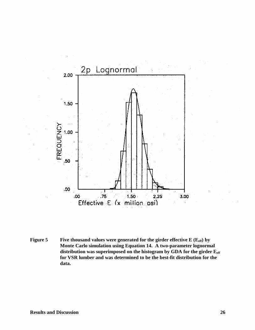
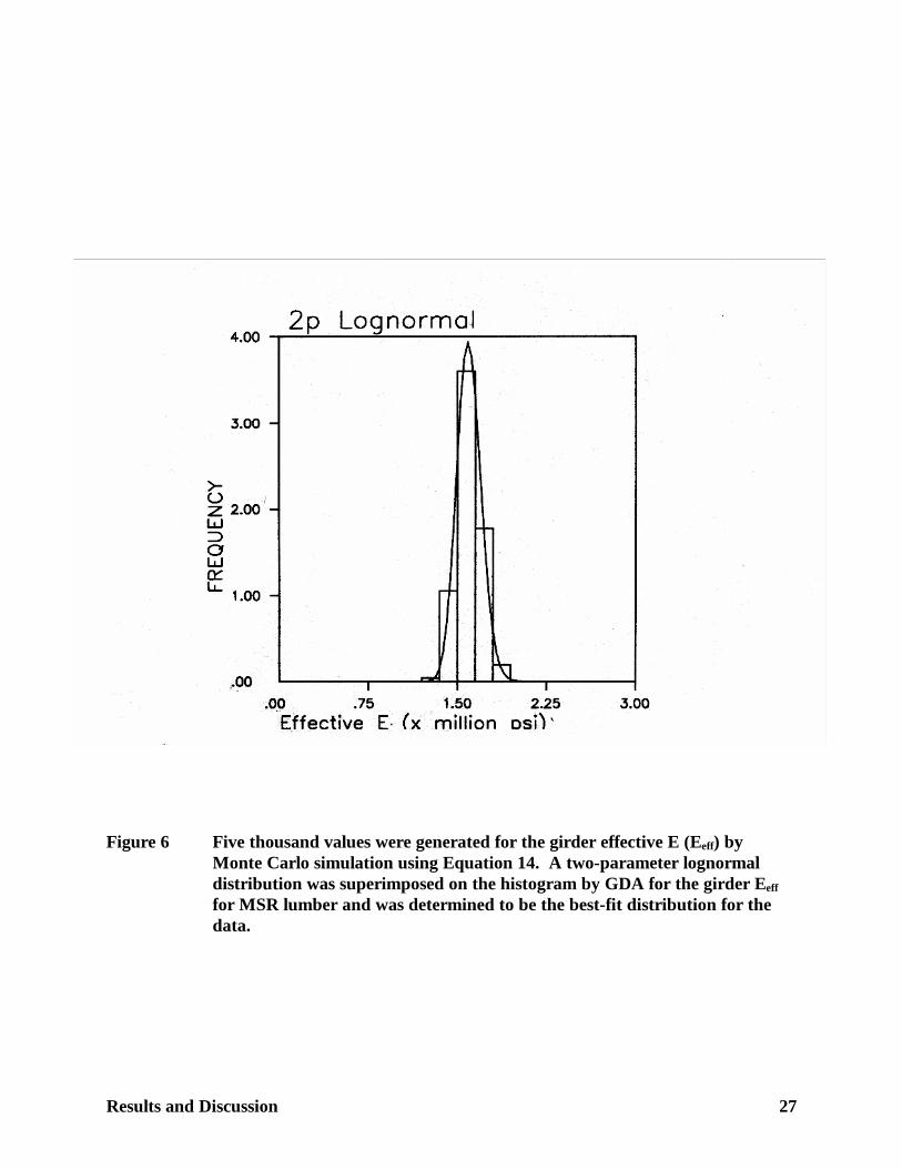
In Figure 5 and in Figure 6, the two-parameter lognormal distribution fit the data well based
collectively on the visual test, the maximum log-likelihood, and the Chi-Square test. The
distribution for the effective girder E, Eeff, for MSR lumber (Figure 6) was less variable than the
Eeff distribution for VSR lumber (Figure 5) and this result was expected. When comparing the
Eeff distribution for VSR lumber in Figure 5 against the E-distribution in Figure 1, an averaging
effect can be observed in Figure 5. This same effect occurs for MSR lumber (Figure 6) when the
Eeff distribution is compared with Figure 2.
The distribution for Eeff has a lower coefficient of variation (Ω) for both MSR and VSR lumber.
The standard deviation of Eeff can be calculated using Equation 14 and it is given by
3EEΩ
(16)
Results and Discussion 26
Figure 5 Five thousand values were generated for the girder effective E (Eeff) by Monte Carlo simulation using Equation 14. A two-parameter lognormal distribution was superimposed on the histogram by GDA for the girder Eeff for VSR lumber and was determined to be the best-fit distribution for the data.
Results and Discussion 27
Figure 6 Five thousand values were generated for the girder effective E (Eeff) by Monte Carlo simulation using Equation 14. A two-parameter lognormal distribution was superimposed on the histogram by GDA for the girder Eeff for MSR lumber and was determined to be the best-fit distribution for the data.
Results and Discussion 28
The coefficient of variation of Eeff is therefore
3
3 E
E
E
E
Ω=
Ω
(17)
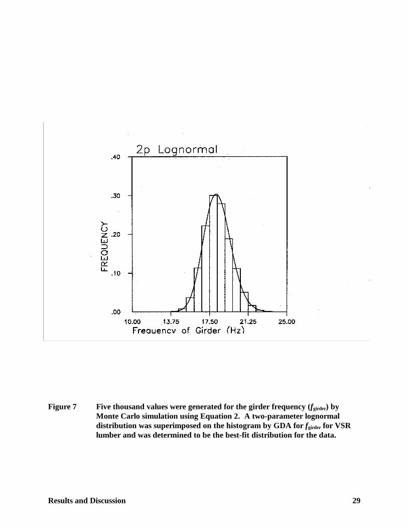
The two-parameter lognormal distribution fitted the data well for girder frequency (Figure 7 and
Figure 8) based collectively on the visual test, the maximum log-likelihood, the Chi-Squared Test,
and the Kolmogorov-Smirnov test. The girder frequency distribution for MSR lumber (Figure 8)
was less variable than the distribution for VSR lumber (Figure 7). Upon inspection of Figure 7
and Figure 8, the probability that the frequency of the girder is less than 10 Hz would be zero for
each case.
For the frequency of the floor system, the normal distribution fit the data well for VSR lumber
(Figure 9) and MSR lumber (Figure 10) based collectively on the visual test, the maximum log-
likelihood, the Chi-Squared test, and the Kolmogorov-Smirnov test. The system frequency
distribution for MSR lumber (Figure 10) was also less variable than the system frequency
distribution for VSR lumber (Figure 9). The probability that the system frequency is less than 10
Hz for VSR lumber (Figure 9) is 0.0537 while the same probability for MSR lumber (Figure 10) is
zero. The first percentile of VSR lumber and MSR lumber is 9.34 Hz and 10.60 Hz, respectively.
The difference between the first percentile values using Equation 1 is about 13 percent, which is
caused by differences in ΩE.
Results and Discussion 29
Figure 7 Five thousand values were generated for the girder frequency (fgirder) by Monte Carlo simulation using Equation 2. A two-parameter lognormal distribution was superimposed on the histogram by GDA for fgirder for VSR lumber and was determined to be the best-fit distribution for the data.
Results and Discussion 30
Figure 8 Five thousand values were generated for the girder frequency (fgirder) by Monte Carlo simulation using Equation 2. A two-parameter lognormal distribution was superimposed on the histogram by GDA for fgirder for MSR lumber and was determined to be the best-fit distribution for the data.
Results and Discussion 31
Figure 9 Five thousand values were generated for the floor system frequency (fsystem) byMonte Carlo simulation using Equation 3. A normal distribution was superimposed on the histogram by GDA for fsystem for VSR lumber and was determined to be the best-fit distribution for the data.
Results and Discussion 32
Figure 10 Five thousand values were generated for the floor system frequency (fsystem) byMonte Carlo simulation using Equation 3. A normal distribution was superimposed on the histogram by GDA for fsystem for MSR lumber and was determined to be the best-fit distribution for the data.
Results and Discussion 33
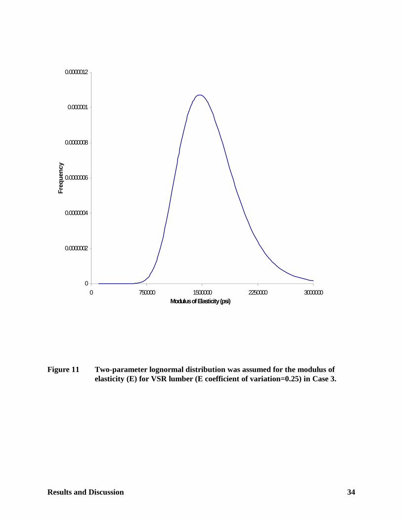
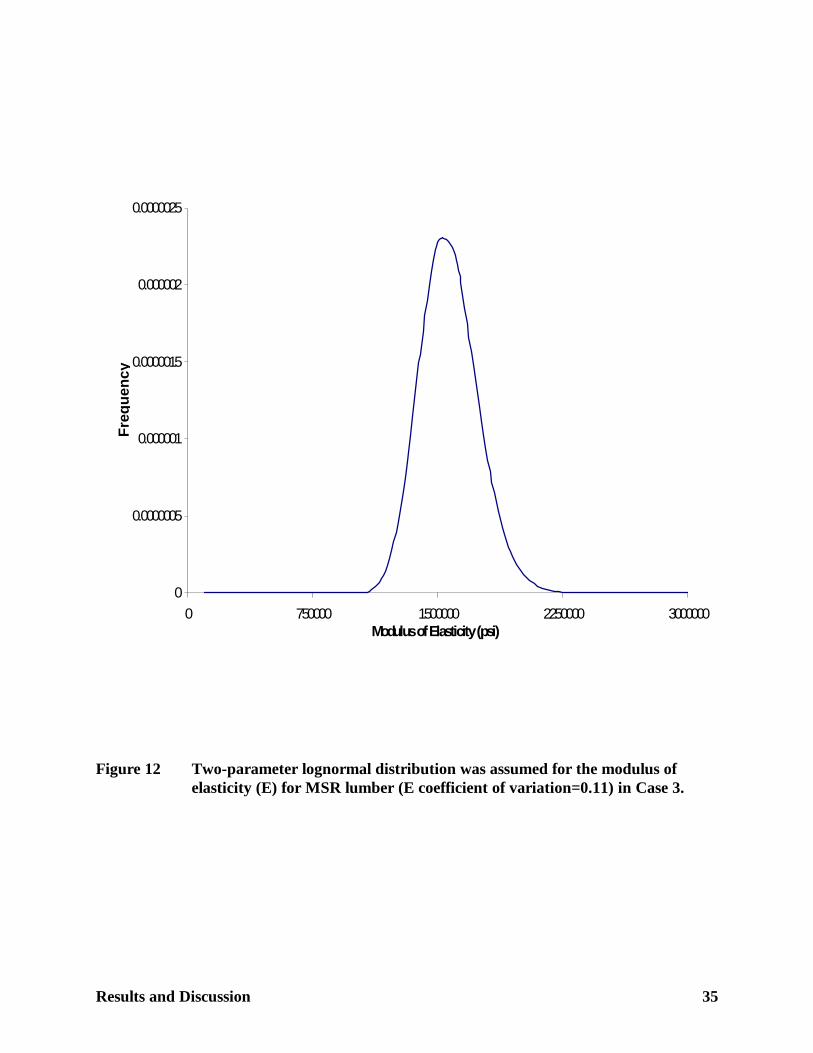
Case 3
Results for the E-distribution for both MSR and VSR lumber (Figure 11 and Figure 12) are
identical to the results given for the E-distribution for Case 1. They are identical to Case 1
because the values used to calculate the parameters for the E-distribution in Equations 5 and 6 did
not change across floor cases. These values remained constant throughout the floor cases
studied. The only variable that did change was ΩE.
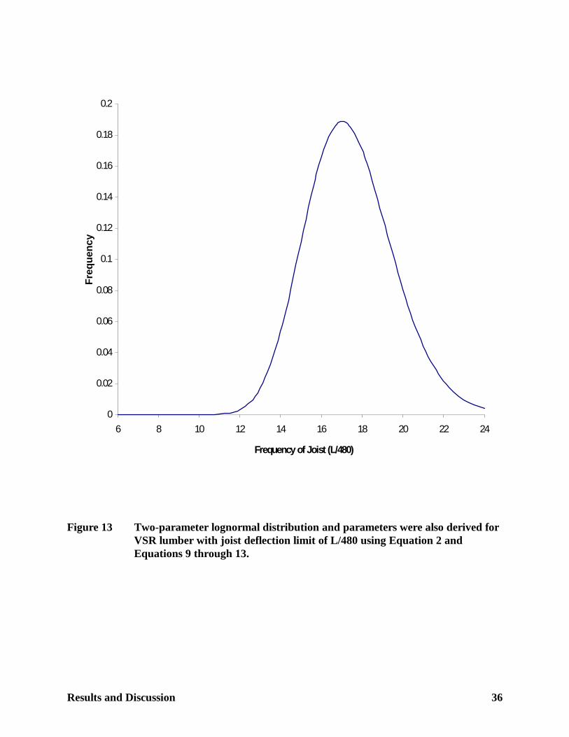
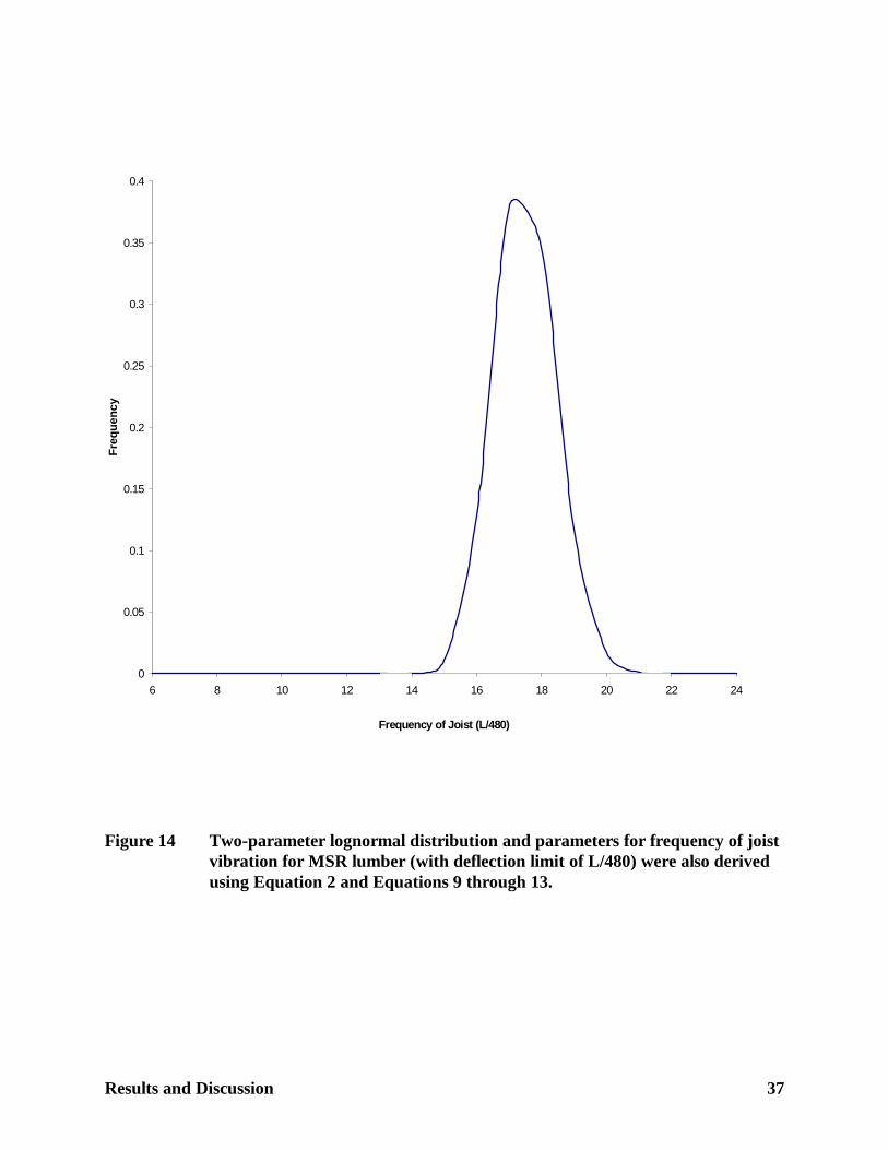
Results for the frequency distribution differed from the results for the frequency distribution in
Case 1 because the joists were designed to a stricter deflection limit (L/ 480). The frequency
distribution for both MSR and VSR lumber shifted to the right which resulted in better expected
vibrational performance than in Case 1. The calculated frequency distribution of a joist for VSR
lumber is shown in Figure 13. The predicted frequency is lognormally distributed because E was
assumed to be lognormal. The calculated frequency distribution for MSR lumber is represented in
Figure 14 and it is also lognormally distributed. The frequency distribution in Figure 14 for MSR
lumber is also noticeably less variable than the frequency distribution for VSR lumber in
Figure 13.
The probability that the frequency is less than 10 Hz in Figure 13 is practically zero.
Theoretically, the lognormal density functions starts at zero, thus some very small area exists
between 0.0 and 10.0. Hereafter, this case will be referred to as zero area. The first percentile of
the distribution is 12.98. For Figure 14, the probability that the frequency is less than 10 Hz is
also zero. The first percentile of the frequency distribution for MSR lumber is 15.36 which is 18
Results and Discussion 34
Figure 11 Two-parameter lognormal distribution was assumed for the modulus of elasticity (E) for VSR lumber (E coefficient of variation=0.25) in Case 3.
0
0.0000002
0.0000004
0.0000006
0.0000008
0.000001
0.0000012
0 750000 1500000 2250000 3000000 Modulus of Elasticity (psi)
Fre
quen
cy
Results and Discussion 35
Figure 12 Two-parameter lognormal distribution was assumed for the modulus of elasticity (E) for MSR lumber (E coefficient of variation=0.11) in Case 3.
0
0.0000005
0.000001
0.0000015
0.000002
0.0000025
0 750000 1500000 2250000 3000000Modulus of Elasticity (psi)
Fre
que
ncy
Results and Discussion 36
Figure 13 Two-parameter lognormal distribution and parameters were also derived for VSR lumber with joist deflection limit of L/480 using Equation 2 and Equations 9 through 13.
0
0.02
0.04
0.06
0.08
0.1
0.12
0.14
0.16
0.18
0.2
6 8 10 12 14 16 18 20 22 24
Frequency of Joist (L/480)
Fre
quen
cy
Results and Discussion 37
Figure 14 Two-parameter lognormal distribution and parameters for frequency of joist vibration for MSR lumber (with deflection limit of L/480) were also derived using Equation 2 and Equations 9 through 13.
0
0.05
0.1
0.15
0.2
0.25
0.3
0.35
0.4
6 8 10 12 14 16 18 20 22 24
Frequency of Joist (L/480)
Fre
quen
cy
Results and Discussion 38
percent more than the first percentile for VSR lumber according to Equation 1. In other words,
the expected vibrational performance for MSR lumber in this case is 18 percent better than VSR
lumber.
Case 4
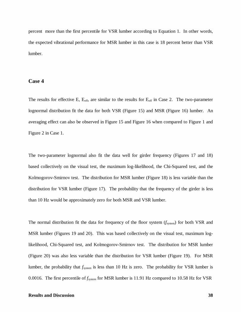
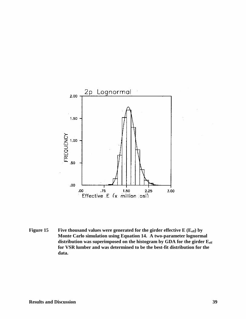
The results for effective E, Eeff, are similar to the results for Eeff in Case 2. The two-parameter
lognormal distribution fit the data for both VSR (Figure 15) and MSR (Figure 16) lumber. An
averaging effect can also be observed in Figure 15 and Figure 16 when compared to Figure 1 and
Figure 2 in Case 1.
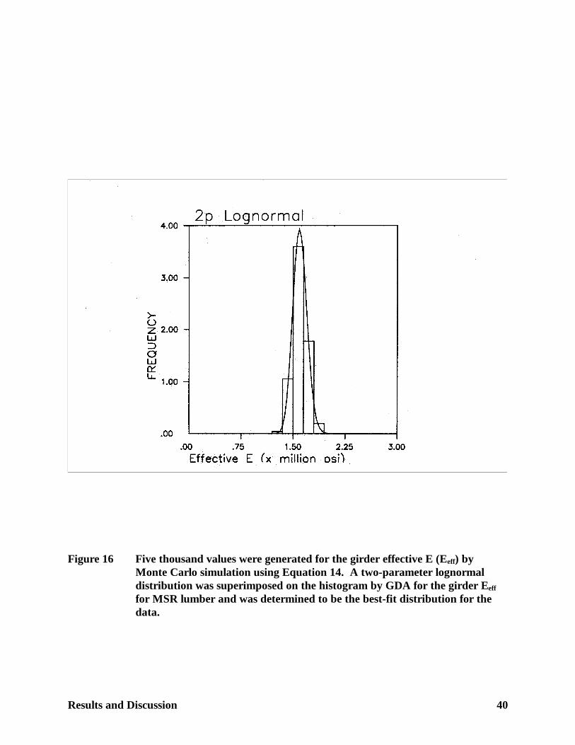
The two-parameter lognormal also fit the data well for girder frequency (Figures 17 and 18)
based collectively on the visual test, the maximum log-likelihood, the Chi-Squared test, and the
Kolmogorov-Smirnov test. The distribution for MSR lumber (Figure 18) is less variable than the
distribution for VSR lumber (Figure 17). The probability that the frequency of the girder is less
than 10 Hz would be approximately zero for both MSR and VSR lumber.
The normal distribution fit the data for frequency of the floor system (fsystem) for both VSR and
MSR lumber (Figures 19 and 20). This was based collectively on the visual test, maximum log-
likelihood, Chi-Squared test, and Kolmogorov-Smirnov test. The distribution for MSR lumber
(Figure 20) was also less variable than the distribution for VSR lumber (Figure 19). For MSR
lumber, the probability that fsystem is less than 10 Hz is zero. The probability for VSR lumber is
0.0016. The first percentile of fsystem for MSR lumber is 11.91 Hz compared to 10.58 Hz for VSR
Results and Discussion 39
Figure 15 Five thousand values were generated for the girder effective E (Eeff) by Monte Carlo simulation using Equation 14. A two-parameter lognormal distribution was superimposed on the histogram by GDA for the girder Eeff for VSR lumber and was determined to be the best-fit distribution for the data.
Results and Discussion 40
Figure 16 Five thousand values were generated for the girder effective E (Eeff) by Monte Carlo simulation using Equation 14. A two-parameter lognormal distribution was superimposed on the histogram by GDA for the girder Eeff for MSR lumber and was determined to be the best-fit distribution for the data.
Results and Discussion 41
Figure 17 Five thousand values were generated for the girder frequency (fgirder) Monte Carlo simulation using Equation 2. A two-parameter lognormal distribution was superimposed on the histogram by GDA for fgirder for VSR lumber and was determined to be the best-fit distribution for the data.
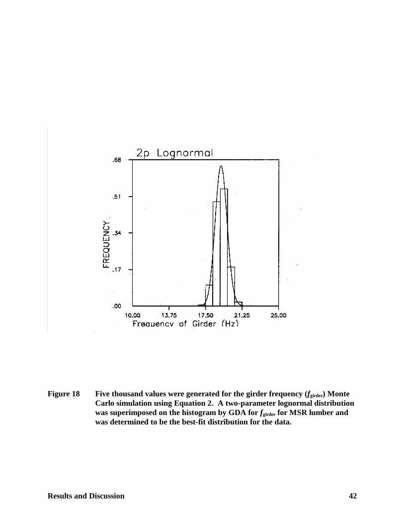
Results and Discussion 42
Figure 18 Five thousand values were generated for the girder frequency (fgirder) Monte Carlo simulation using Equation 2. A two-parameter lognormal distribution was superimposed on the histogram by GDA for fgirder for MSR lumber and was determined to be the best-fit distribution for the data.
Results and Discussion 43
Figure 19 Five thousand values were generated for the floor system frequency (fsystem) byMonte Carlo simulation using Equation 3. A normal distribution was superimposed on the histogram by GDA for fsystem for VSR lumber and was determined to be the best-fit distribution for the data.
Results and Discussion 44
Figure 20 Five thousand values were generated for the floor system frequency (fsystem) byMonte Carlo simulation using Equation 3. A normal distribution was superimposed on the histogram by GDA for fsystem for MSR lumber and was determined to be the best-fit distribution for the data.
Results and Discussion 45
lumber. The ratio of the first percentile of MSR lumber to the first percentile of VSR lumber is
1.13 which indicates that an MSR lumber floor system will have better floor performance than
VSR lumber by 13 percent.
A limit on fsystem for good floor performance has been proposed by Shue (1995) for continuous
girders. The 13 percent difference between first percentiles for MSR and VSR lumber in Case 4
may be significant. Based on in-situ tests, he first calculated fsystem based on the clear span
between points of support and the prediction did not correlate well with measured results. He
then determined that the span between points of inflection produced results that correlated better
with the measured floor vibrational response.
In comparing the girder frequency and system frequency in Case 4 with the corresponding
distributions in Case 2, the distributions in Case 4 are slightly shifted more to the right. This shift
to the right in Case 4 can be attributed to the joists and girder being designed to a more strict
deflection limit (L/480 and L/600, respectively).
Case 5 (Load Sharing)
The two-parameter lognormal distribution fit the data well in Figures 21 and 22 for effective joist
E, Ej, based collectively on the visual test, maximum log-likelihood, Chi-Squared test, and
Kolmogorov-Smirnov test. Again, MSR lumber effective joist E based on Equation 15 (Figure
22) is less variable than VSR lumber effective joist E (Figure 21).
Results and Discussion 46
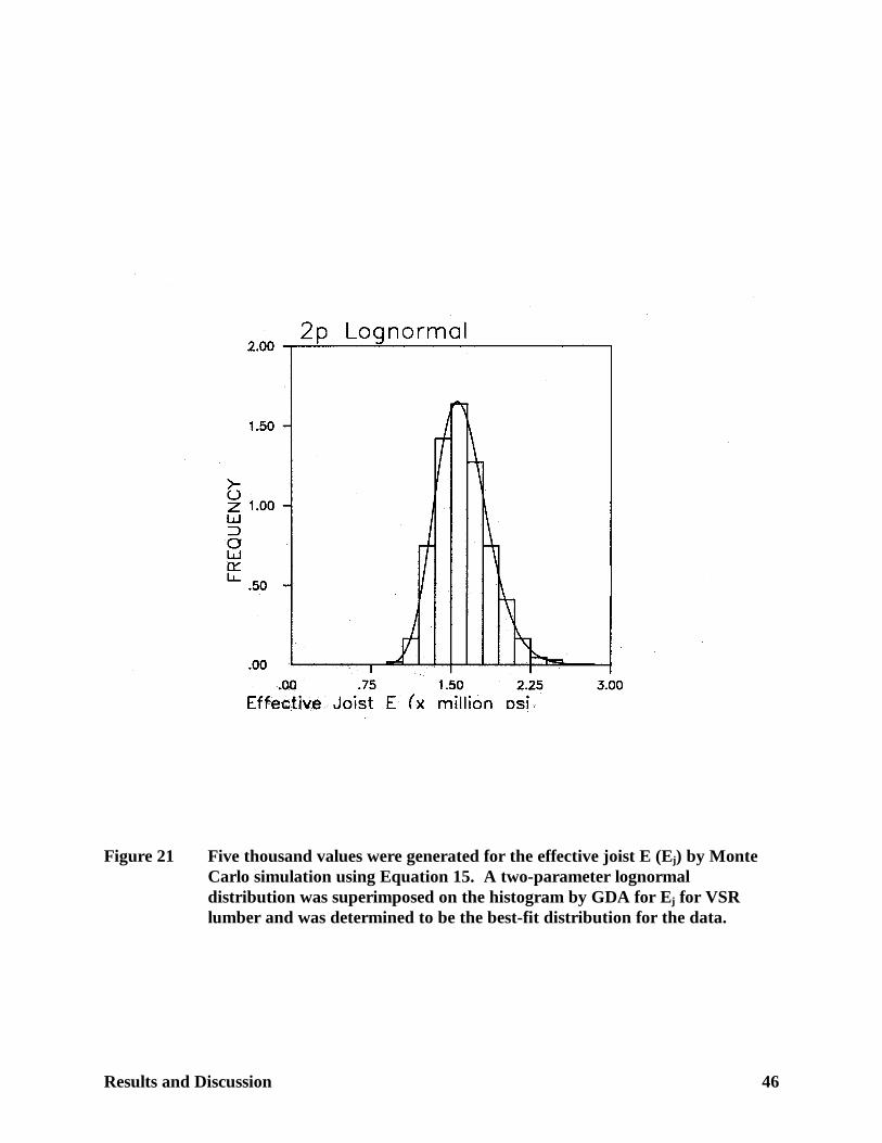
Figure 21 Five thousand values were generated for the effective joist E (Ej) by Monte Carlo simulation using Equation 15. A two-parameter lognormal distribution was superimposed on the histogram by GDA for Ej for VSR lumber and was determined to be the best-fit distribution for the data.
Results and Discussion 47
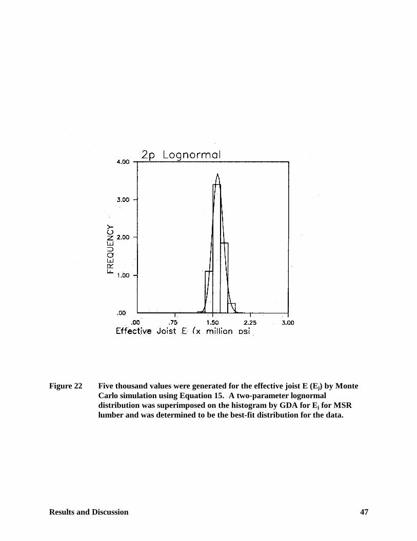
Figure 22 Five thousand values were generated for the effective joist E (Ej) by Monte Carlo simulation using Equation 15. A two-parameter lognormal distribution was superimposed on the histogram by GDA for Ej for MSR lumber and was determined to be the best-fit distribution for the data.
Results and Discussion 48
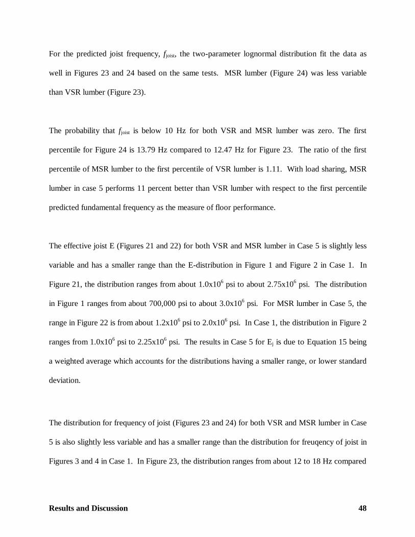
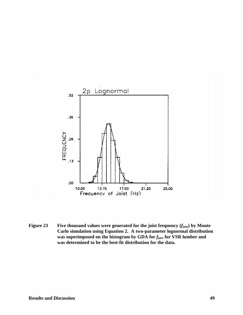
For the predicted joist frequency, fjoist, the two-parameter lognormal distribution fit the data as
well in Figures 23 and 24 based on the same tests. MSR lumber (Figure 24) was less variable
than VSR lumber (Figure 23).
The probability that fjoist is below 10 Hz for both VSR and MSR lumber was zero. The first
percentile for Figure 24 is 13.79 Hz compared to 12.47 Hz for Figure 23. The ratio of the first
percentile of MSR lumber to the first percentile of VSR lumber is 1.11. With load sharing, MSR
lumber in case 5 performs 11 percent better than VSR lumber with respect to the first percentile
predicted fundamental frequency as the measure of floor performance.
The effective joist E (Figures 21 and 22) for both VSR and MSR lumber in Case 5 is slightly less
variable and has a smaller range than the E-distribution in Figure 1 and Figure 2 in Case 1. In
Figure 21, the distribution ranges from about 1.0x10⁶ psi to about 2.75x10⁶ psi. The distribution
in Figure 1 ranges from about 700,000 psi to about 3.0x10⁶ psi. For MSR lumber in Case 5, the
range in Figure 22 is from about 1.2x10⁶ psi to 2.0x10⁶ psi. In Case 1, the distribution in Figure 2
ranges from 1.0x10⁶ psi to 2.25x10⁶ psi. The results in Case 5 for Ej is due to Equation 15 being
a weighted average which accounts for the distributions having a smaller range, or lower standard
deviation.
The distribution for frequency of joist (Figures 23 and 24) for both VSR and MSR lumber in Case
5 is also slightly less variable and has a smaller range than the distribution for freuqency of joist in
Figures 3 and 4 in Case 1. In Figure 23, the distribution ranges from about 12 to 18 Hz compared
Results and Discussion 49
Figure 23 Five thousand values were generated for the joist frequency (f joist) by Monte Carlo simulation using Equation 2. A two-parameter lognormal distribution was superimposed on the histogram by GDA for f joist for VSR lumber and was determined to be the best-fit distribution for the data.
Results and Discussion 50
Figure 24 Five thousand values were generated for the joist frequency (f joist) by Monte Carlo simulation using Equation 2. A two-parameter lognormal distribution was superimposed on the histogram by GDA for f joist for MSR lumber and was determined to be the best-fit distribution for the data.
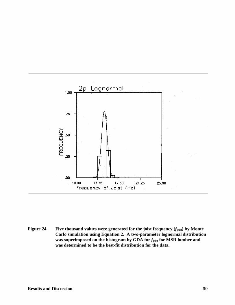
Results and Discussion 51
to the range of 9 to 23 Hz in Figure 3 for Case 1. For MSR lumber (Figure 24) in Case 5, the
range is 13 to 16 Hz compared to the range for MSR lumber (Figure 4) in Case 1 of 12 to 18 Hz.
Case 6 (Load Sharing)
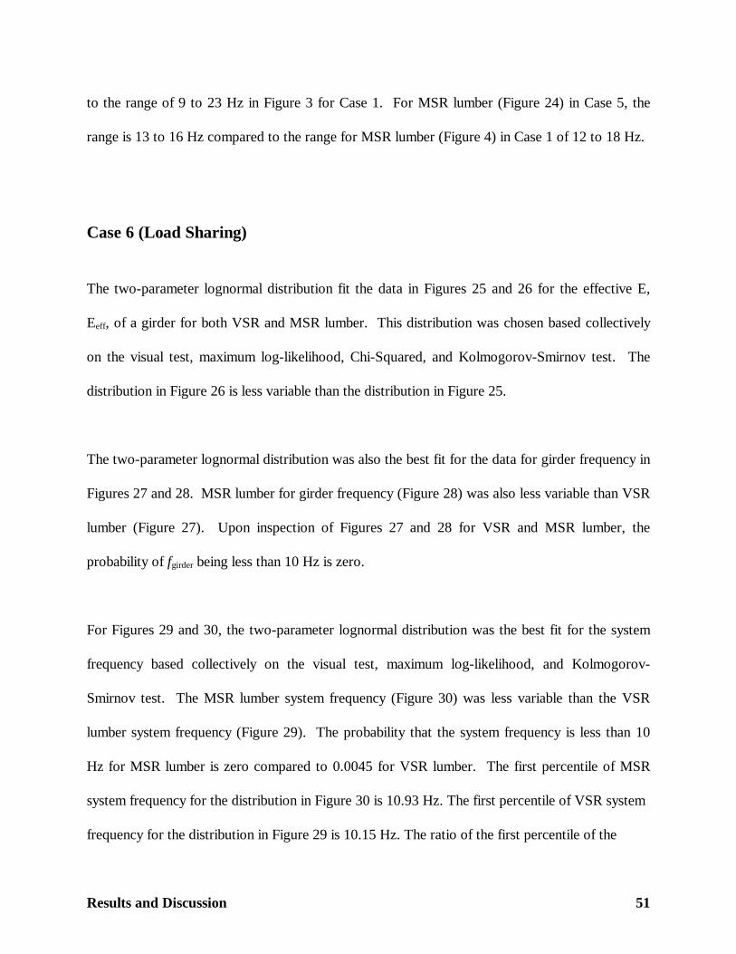
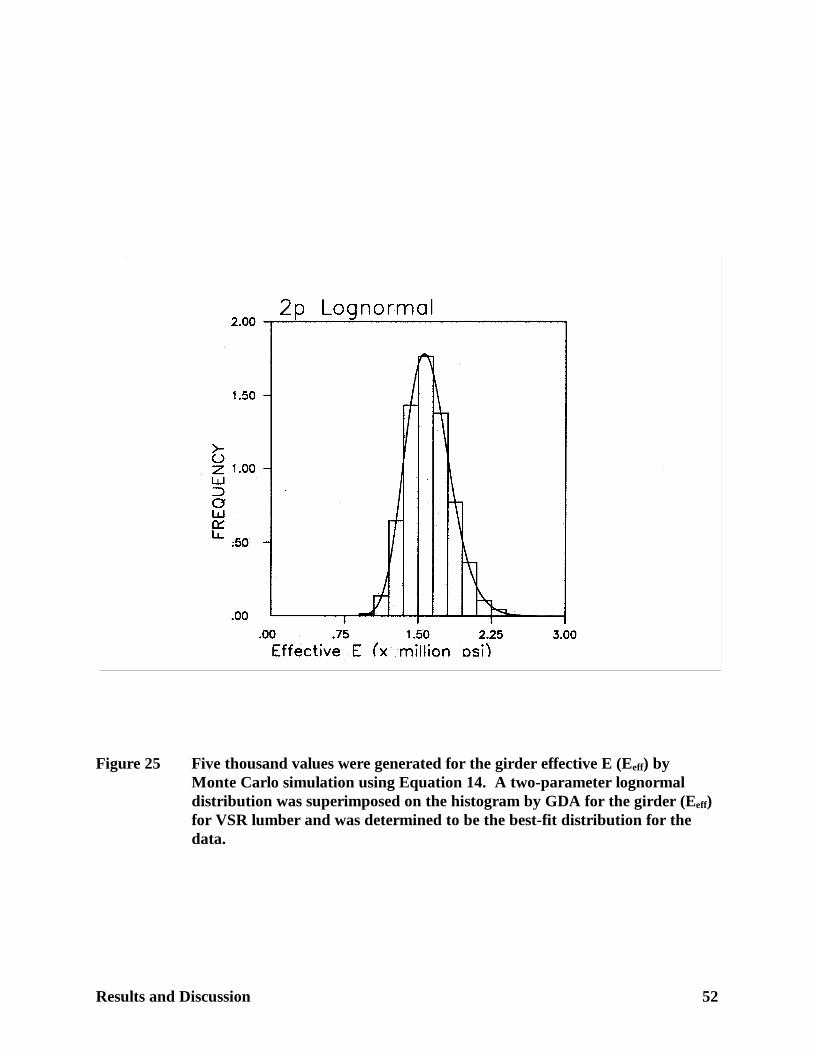
The two-parameter lognormal distribution fit the data in Figures 25 and 26 for the effective E,
Eeff, of a girder for both VSR and MSR lumber. This distribution was chosen based collectively
on the visual test, maximum log-likelihood, Chi-Squared, and Kolmogorov-Smirnov test. The
distribution in Figure 26 is less variable than the distribution in Figure 25.
The two-parameter lognormal distribution was also the best fit for the data for girder frequency in
Figures 27 and 28. MSR lumber for girder frequency (Figure 28) was also less variable than VSR
lumber (Figure 27). Upon inspection of Figures 27 and 28 for VSR and MSR lumber, the
probability of fgirder being less than 10 Hz is zero.
For Figures 29 and 30, the two-parameter lognormal distribution was the best fit for the system
frequency based collectively on the visual test, maximum log-likelihood, and Kolmogorov-
Smirnov test. The MSR lumber system frequency (Figure 30) was less variable than the VSR
lumber system frequency (Figure 29). The probability that the system frequency is less than 10
Hz for MSR lumber is zero compared to 0.0045 for VSR lumber. The first percentile of MSR
system frequency for the distribution in Figure 30 is 10.93 Hz. The first percentile of VSR system
frequency for the distribution in Figure 29 is 10.15 Hz. The ratio of the first percentile of the
Results and Discussion 52
Figure 25 Five thousand values were generated for the girder effective E (Eeff) by Monte Carlo simulation using Equation 14. A two-parameter lognormal distribution was superimposed on the histogram by GDA for the girder (Eeff) for VSR lumber and was determined to be the best-fit distribution for the data.
Results and Discussion 53
Figure 26 Five thousand values were generated for the girder effective E (Eeff) by Monte Carlo simulation using Equation 14. A two-parameter lognormal distribution was superimposed on the histogram by GDA for the girder (Eeff) for MSR lumber and was determined to be the best-fit distribution for the data.
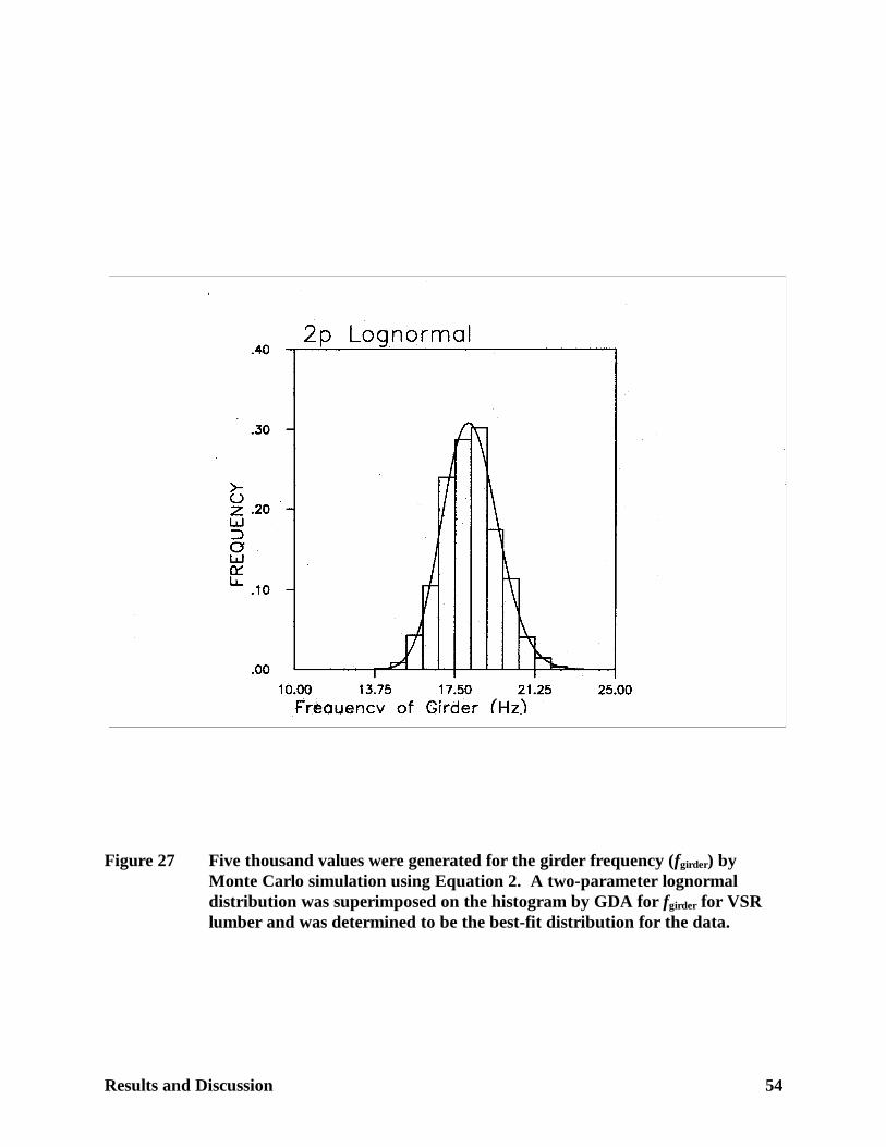
Results and Discussion 54
Figure 27 Five thousand values were generated for the girder frequency (fgirder) by Monte Carlo simulation using Equation 2. A two-parameter lognormal distribution was superimposed on the histogram by GDA for fgirder for VSR lumber and was determined to be the best-fit distribution for the data.
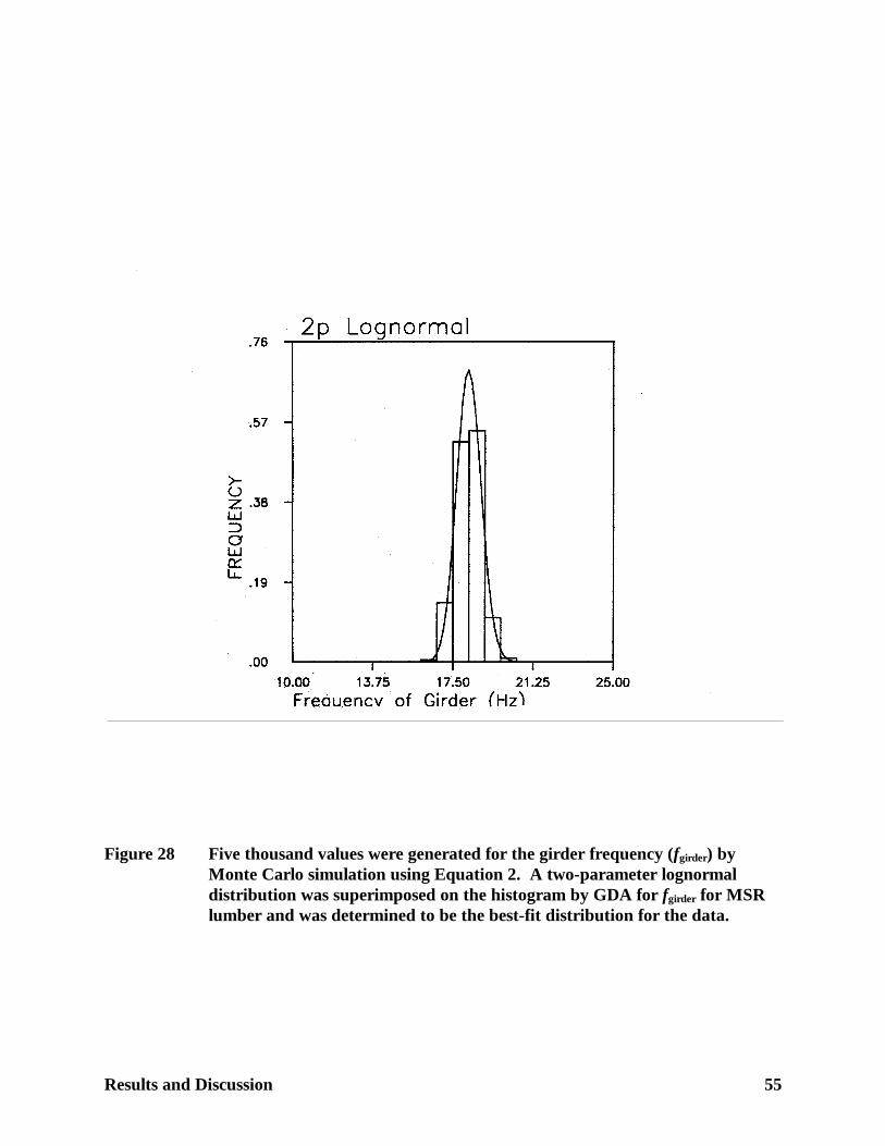
Results and Discussion 55
Figure 28 Five thousand values were generated for the girder frequency (fgirder) by Monte Carlo simulation using Equation 2. A two-parameter lognormal distribution was superimposed on the histogram by GDA for fgirder for MSR lumber and was determined to be the best-fit distribution for the data.
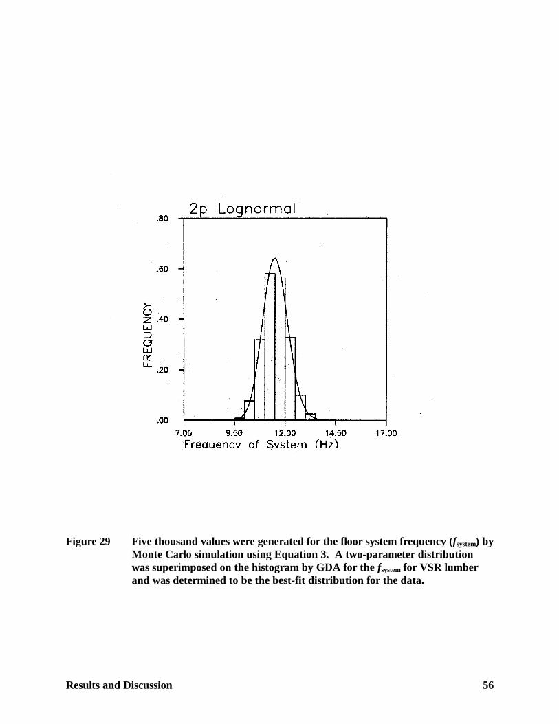
Results and Discussion 56
Figure 29 Five thousand values were generated for the floor system frequency (fsystem) byMonte Carlo simulation using Equation 3. A two-parameter distribution was superimposed on the histogram by GDA for the fsystem for VSR lumber and was determined to be the best-fit distribution for the data.
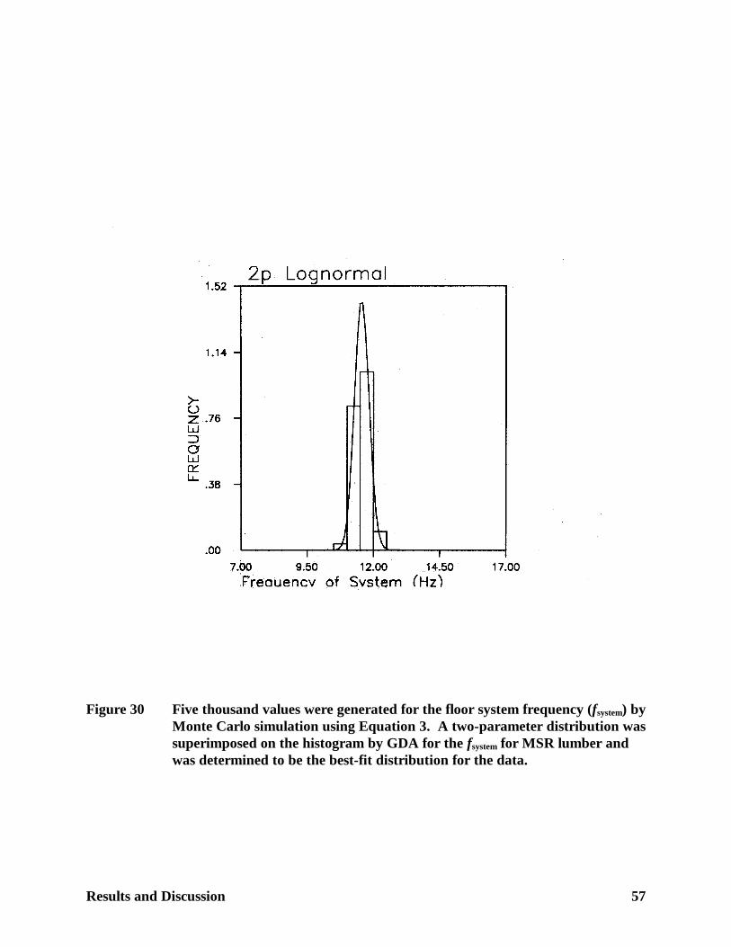
Results and Discussion 57
Figure 30 Five thousand values were generated for the floor system frequency (fsystem) byMonte Carlo simulation using Equation 3. A two-parameter distribution wassuperimposed on the histogram by GDA for the fsystem for MSR lumber and was determined to be the best-fit distribution for the data.
Results and Discussion 58
predicted system frequency for MSR lumber to the corresponding first percentile of VSR lumber
was 1.08 which means that the MSR floor system with load sharing included has an 8 percent
better predicted vibrational performance over a VSR floor system.
The fsystem distributions in Case 6 (Figures 29 and 30) are less variable than the fsystem distributions
(Figures 9 and 10) in Case 2. The first percentile values of fsystem for MSR and VSR lumber in
Case 6 are larger than the first percentile values for MSR and VSR lumber in Case 2.
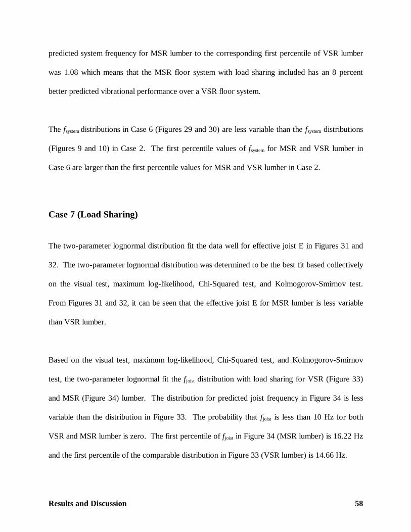
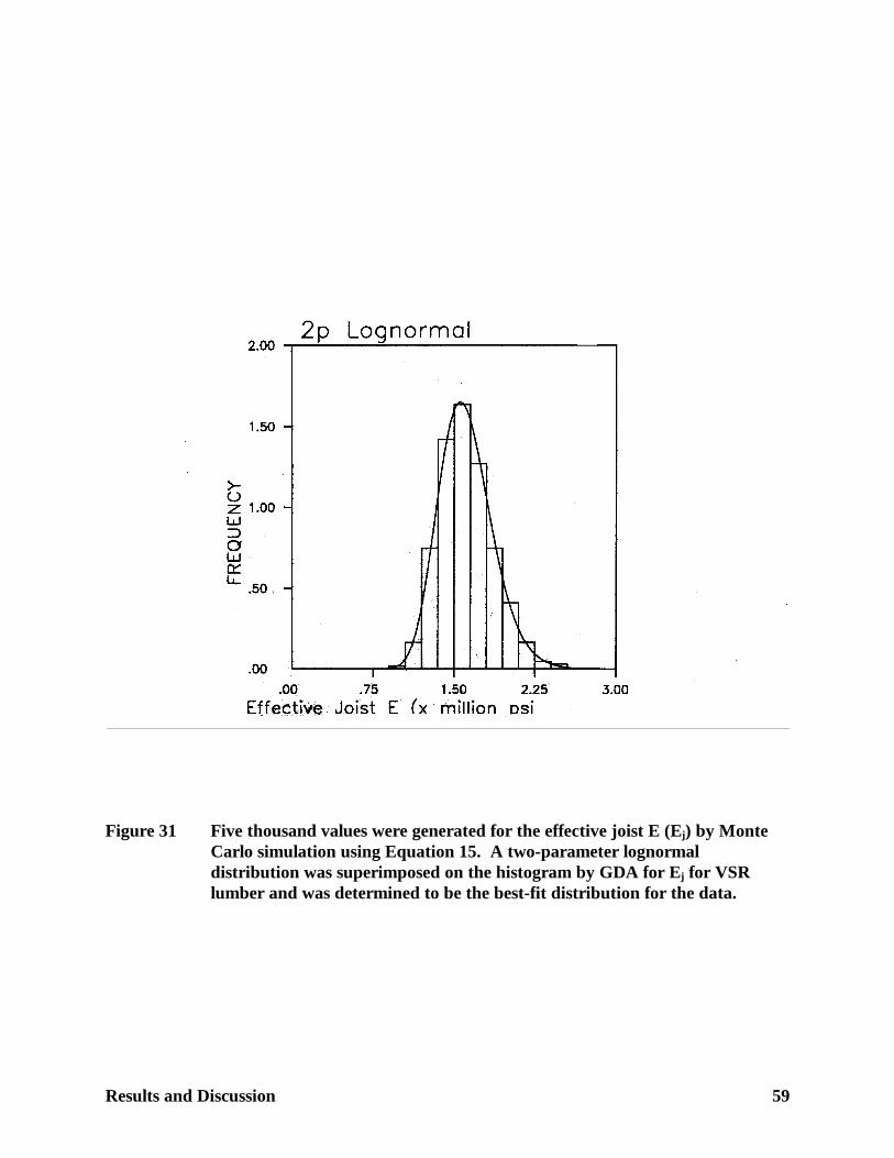
Case 7 (Load Sharing)
The two-parameter lognormal distribution fit the data well for effective joist E in Figures 31 and
32. The two-parameter lognormal distribution was determined to be the best fit based collectively
on the visual test, maximum log-likelihood, Chi-Squared test, and Kolmogorov-Smirnov test.
From Figures 31 and 32, it can be seen that the effective joist E for MSR lumber is less variable
than VSR lumber.
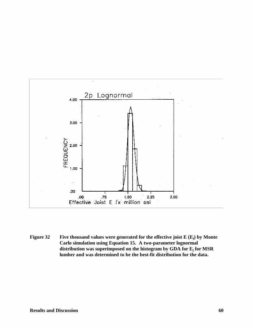
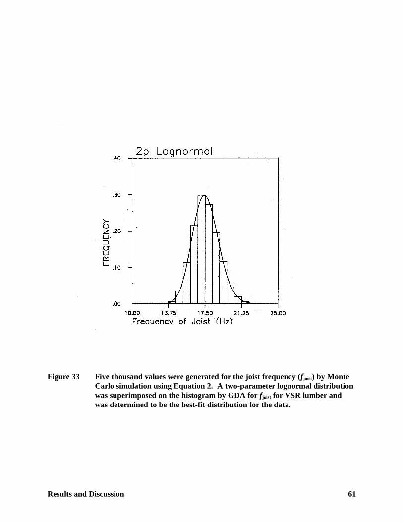
Based on the visual test, maximum log-likelihood, Chi-Squared test, and Kolmogorov-Smirnov
test, the two-parameter lognormal fit the fjoist distribution with load sharing for VSR (Figure 33)
and MSR (Figure 34) lumber. The distribution for predicted joist frequency in Figure 34 is less
variable than the distribution in Figure 33. The probability that fjoist is less than 10 Hz for both
VSR and MSR lumber is zero. The first percentile of fjoist in Figure 34 (MSR lumber) is 16.22 Hz
and the first percentile of the comparable distribution in Figure 33 (VSR lumber) is 14.66 Hz.
Results and Discussion 59
Figure 31 Five thousand values were generated for the effective joist E (Ej) by Monte Carlo simulation using Equation 15. A two-parameter lognormal distribution was superimposed on the histogram by GDA for Ej for VSR lumber and was determined to be the best-fit distribution for the data.
Results and Discussion 60
Figure 32 Five thousand values were generated for the effective joist E (Ej) by Monte Carlo simulation using Equation 15. A two-parameter lognormal distribution was superimposed on the histogram by GDA for Ej for MSR lumber and was determined to be the best-fit distribution for the data.
Results and Discussion 61
Figure 33 Five thousand values were generated for the joist frequency (f joist) by Monte Carlo simulation using Equation 2. A two-parameter lognormal distribution was superimposed on the histogram by GDA for f joist for VSR lumber and was determined to be the best-fit distribution for the data.
Results and Discussion 62
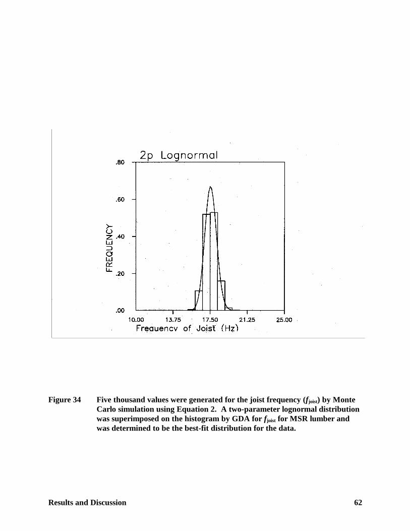
Figure 34 Five thousand values were generated for the joist frequency (f joist) by Monte Carlo simulation using Equation 2. A two-parameter lognormal distribution was superimposed on the histogram by GDA for f joist for MSR lumber and was determined to be the best-fit distribution for the data.
Results and Discussion 63
The ratio of these two numbers using equation 1 is 1.11 which reveals that MSR lumber has a
better predicted vibrational performance than VSR lumber by 11 percent.
The results for fjoist in Case 7 are better compared to the results for fjoist in Case 5. The fjoist
distributions in Figures 33 and 34 are shifted to the right more compared to the fjoist distributions
in Figures 23 and 24.
In comparison with Case 3, Case 7 had better results because the first percentile values of fjoist for
MSR and VSR lumber are higher than the first percentile values of fjoist for MSR and VSR lumber
in Case 3. Case 3 did not include a load sharing component, whereas Case 7 included a load
sharing model which should predict more realistic floor behavior.
Case 8 (Load Sharing)
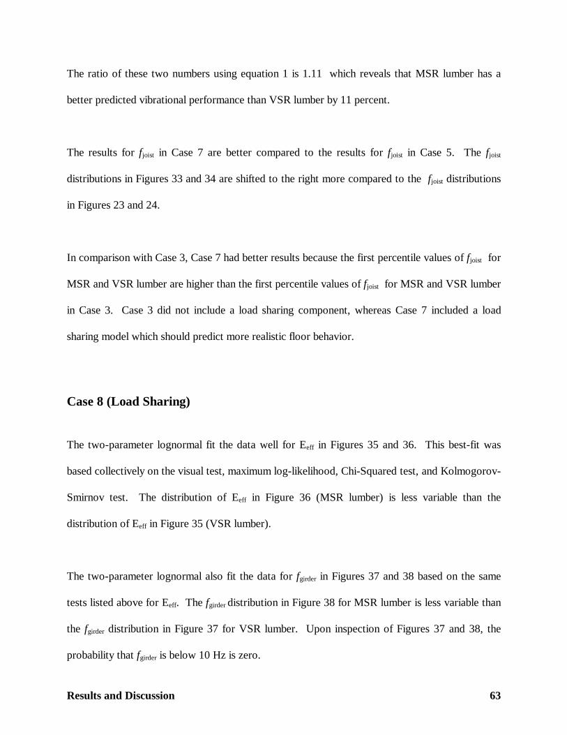
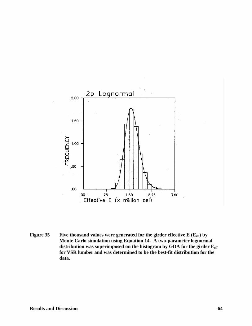
The two-parameter lognormal fit the data well for Eeff in Figures 35 and 36. This best-fit was
based collectively on the visual test, maximum log-likelihood, Chi-Squared test, and Kolmogorov-
Smirnov test. The distribution of Eeff in Figure 36 (MSR lumber) is less variable than the
distribution of Eeff in Figure 35 (VSR lumber).
The two-parameter lognormal also fit the data for fgirder in Figures 37 and 38 based on the same
tests listed above for Eeff. The fgirder distribution in Figure 38 for MSR lumber is less variable than
the fgirder distribution in Figure 37 for VSR lumber. Upon inspection of Figures 37 and 38, the
probability that fgirder is below 10 Hz is zero.
Results and Discussion 64
Figure 35 Five thousand values were generated for the girder effective E (Eeff) by Monte Carlo simulation using Equation 14. A two-parameter lognormal distribution was superimposed on the histogram by GDA for the girder Eeff for VSR lumber and was determined to be the best-fit distribution for the data.
Results and Discussion 65
`
Figure 36 Five thousand values were generated for the girder effective E (Eeff) by Monte Carlo simulation using Equation 14. A two-parameter lognormal distribution was superimposed on the histogram by GDA for the girder Eeff for MSR lumber and was determined to be the best-fit distribution for the data.
Results and Discussion 66
Figure 37 Five thousand values were generated for the girder frequency (fgirder) by Monte Carlo simulation using Equation 2. A two-parameter lognormal distribution was superimposed on the histogram by GDA for fgirder for VSR lumber and was determined to be the best-fit distribution for the data.
Results and Discussion 67
Figure 38 Five thousand values were generated for the girder frequency (fgirder) by Monte Carlo simulation using Equation 2. A two-parameter lognormal distribution was superimposed on the histogram by GDA for fgirder for MSR lumber and was determined to be the best-fit distribution for the data.

Results and Discussion 68
The two-parameter lognormal fit the data for fsystem for both VSR (Figure 39) and MSR
(Figure 40) lumber. The fsystem distribution in Figure 40 is less variable than the fsystem distribution
in Figure 39. The probability of fsystem less than 10 Hz is zero for both MSR and VSR lumber.
The first percentile for Figure 39 (VSR lumber) is 11.38 Hz and the first percentile for Figure 40
(MSR lumber) is 12.24 Hz. The ratio of the first percentile of MSR lumber to the first percentile
of VSR lumber is 1.08. The predicted floor vibrational performance of MSR lumber based on the
first percentile of frequency is 8 percent better than the predicted floor vibrational performance of
VSR lumber.
The floor system frequency in Case 8 for both VSR and MSR lumber is an improvement over the
floor system frequency for both VSR and MSR lumber in Case 6 upon comparing Figures 39 and
40 versus Figures 29 and 30. The distributions in Figures 39 and 40 are shifted more toward the
right. In addition, the first percentile of fsystem for both MSR and VSR lumber in case 8 are higher
than the first percentile values for MSR and VSR lumber in Case 6.
Results and Discussion 69
Figure 39 Five thousand values were generated for the floor system frequency (fsystem) byMonte Carlo simulation using Equation 3. A two-parameter distribution wassuperimposed on the histogram by GDA for the fsystem for VSR lumber and was determined to be the best-fit distribution for the data.
Results and Discussion 70
Figure 40 Five thousand values were generated for the floor system frequency (fsystem) byMonte Carlo simulation using Equation 3. A two-parameter distribution wassuperimposed on the histogram by GDA for the fsystem for MSR lumber and was determined to be the best-fit distribution for the data.
Summary 71
Summary
An individual joist was studied for Cases 1 through 4 instead of a floor system and thus load
sharing was neglected. The joist in Case 1 was rigidly supported and designed for the L/360 live-
load deflection limit. MSR lumber in Case 1 had an improved vibrational performance over VSR
lumber by 18 percent based on the ratio of the first percentile of the predicted frequency in
Equation 1. The probability that fjoist is less than 10 Hz was close to zero for both VSR and MSR
lumber. However, the MSR lumber floor (ΩE=0.11) had better predicted floor performance
based on the measure of the probability of the joist frequency being less than 10 Hz because its
probability was approximately zero.
When the joist was supported by a girder as in Case 2, ΩE had no detectable positive effect on the
predicted vibrational performance of the floor system. The predicted vibrational performance of
MSR lumber was 13 percent better than the predicted vibrational performance of VSR lumber.
The probability that fsystem is less than 10 Hz for MSR lumber was zero while the same probability
for VSR lumber was 0.0537.
Case 2 provided an example of the potential negative effect of a girder on the vibrational
performance of a floor system. Table 2 provides a summary of the vibrational performance
measures of both floor cases with respect to the ΩE level.
Summary 72
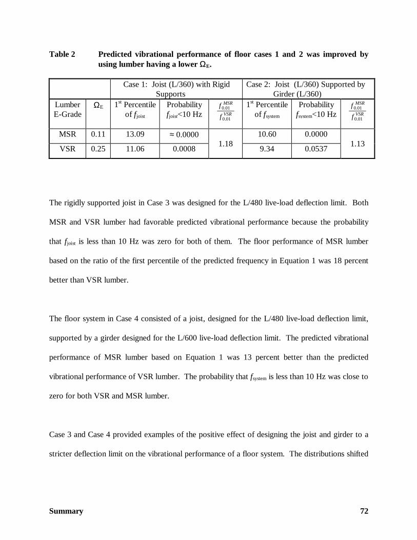
Table 2 Predicted vibrational performance of floor cases 1 and 2 was improved byusing lumber having a lower ΩE.
Case 1: Joist (L/360) with RigidSupports
Case 2: Joist (L/360) Supported byGirder (L/360)
LumberE-Grade
ΩE 1st Percentileof fjoist
Probabilityfjoist<10 Hz VSR
MSR
f
f
01.0
01.0 1st Percentileof fsystem
Probabilityfsystem<10 Hz VSR
MSR
f
f
01.0
01.0
MSR 0.11 13.09 ≈ 0.0000 10.60 0.0000
VSR 0.25 11.06 0.00081.18
9.34 0.05371.13
The rigidly supported joist in Case 3 was designed for the L/480 live-load deflection limit. Both
MSR and VSR lumber had favorable predicted vibrational performance because the probability
that fjoist is less than 10 Hz was zero for both of them. The floor performance of MSR lumber
based on the ratio of the first percentile of the predicted frequency in Equation 1 was 18 percent
better than VSR lumber.
The floor system in Case 4 consisted of a joist, designed for the L/480 live-load deflection limit,
supported by a girder designed for the L/600 live-load deflection limit. The predicted vibrational
performance of MSR lumber based on Equation 1 was 13 percent better than the predicted
vibrational performance of VSR lumber. The probability that fsystem is less than 10 Hz was close to
zero for both VSR and MSR lumber.
Case 3 and Case 4 provided examples of the positive effect of designing the joist and girder to a
stricter deflection limit on the vibrational performance of a floor system. The distributions shifted
Summary 73
to the right and increased the first percentile values in both cases. Table 3 provides a summary of
the measures of performance of both MSR and VSR lumber.
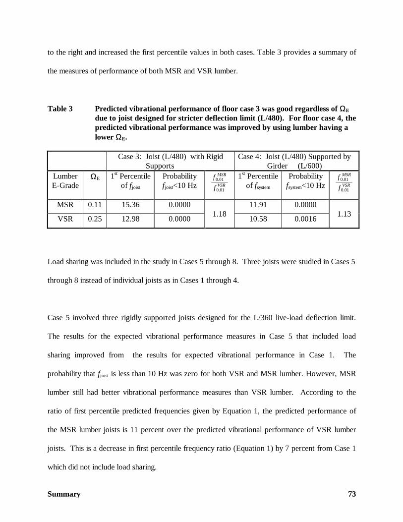
Table 3 Predicted vibrational performance of floor case 3 was good regardless of ΩE due to joist designed for stricter deflection limit (L/480). For floor case 4, thepredicted vibrational performance was improved by using lumber having alower ΩE.
Case 3: Joist (L/480) with RigidSupports
Case 4: Joist (L/480) Supported byGirder (L/600)
LumberE-Grade
ΩE 1st Percentileof fjoist
Probabilityfjoist<10 Hz VSR
MSR
f
f
01.0
01.0 1st Percentileof fsystem
Probabilityfsystem<10 Hz VSR
MSR
f
f
01.0
01.0
MSR 0.11 15.36 0.0000 11.91 0.0000
VSR 0.25 12.98 0.00001.18
10.58 0.00161.13
Load sharing was included in the study in Cases 5 through 8. Three joists were studied in Cases 5
through 8 instead of individual joists as in Cases 1 through 4.
Case 5 involved three rigidly supported joists designed for the L/360 live-load deflection limit.
The results for the expected vibrational performance measures in Case 5 that included load
sharing improved from the results for expected vibrational performance in Case 1. The
probability that fjoist is less than 10 Hz was zero for both VSR and MSR lumber. However, MSR
lumber still had better vibrational performance measures than VSR lumber. According to the
ratio of first percentile predicted frequencies given by Equation 1, the predicted performance of
the MSR lumber joists is 11 percent over the predicted vibrational performance of VSR lumber
joists. This is a decrease in first percentile frequency ratio (Equation 1) by 7 percent from Case 1
which did not include load sharing.
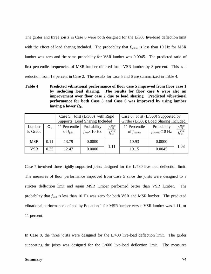
Summary 74
The girder and three joists in Case 6 were both designed for the L/360 live-load deflection limit
with the effect of load sharing included. The probability that fsystem is less than 10 Hz for MSR
lumber was zero and the same probability for VSR lumber was 0.0045. The predicted ratio of
first percentile frequencies of MSR lumber differed from VSR lumber by 8 percent. This is a
reduction from 13 percent in Case 2. The results for case 5 and 6 are summarized in Table 4.
Table 4 Predicted vibrational performance of floor case 5 improved from floor case 1by including load sharing. The results for floor case 6 were also animprovement over floor case 2 due to load sharing. Predicted vibrationalperformance for both Case 5 and Case 6 was improved by using lumberhaving a lower ΩE.
Case 5: Joist (L/360) with RigidSupports; Load Sharing Included
Case 6: Joist (L/360) Supported byGirder (L/360); Load Sharing Included
LumberE-Grade
ΩE 1st Percentileof fjoist
Probabilityfjoist<10 Hz VSR
MSR
f
f
01.0
01.0 1st Percentileof fsystem
Probabilityfsystem<10 Hz VSR
MSR
f
f
01.0
01.0
MSR 0.11 13.79 0.0000 10.93 0.0000
VSR 0.25 12.47 0.00001.11
10.15 0.00451.08
Case 7 involved three rigidly supported joists designed for the L/480 live-load deflection limit.
The measures of floor performance improved from Case 5 since the joists were designed to a
stricter deflection limit and again MSR lumber performed better than VSR lumber. The
probability that fjoist is less than 10 Hz was zero for both VSR and MSR lumber. The predicted
vibrational performance defined by Equation 1 for MSR lumber versus VSR lumber was 1.11, or
11 percent.
In Case 8, the three joists were designed for the L/480 live-load deflection limit. The girder
supporting the joists was designed for the L/600 live-load deflection limit. The measures
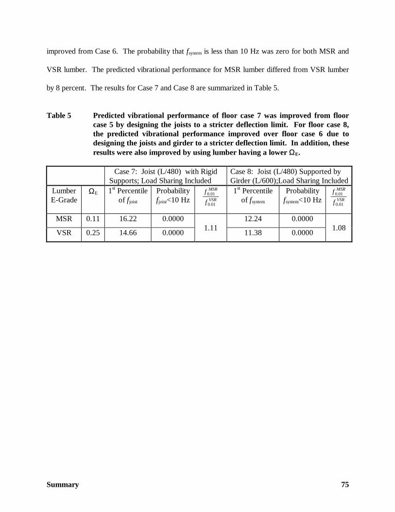
Summary 75
improved from Case 6. The probability that fsystem is less than 10 Hz was zero for both MSR and
VSR lumber. The predicted vibrational performance for MSR lumber differed from VSR lumber
by 8 percent. The results for Case 7 and Case 8 are summarized in Table 5.
Table 5 Predicted vibrational performance of floor case 7 was improved from floorcase 5 by designing the joists to a stricter deflection limit. For floor case 8,the predicted vibrational performance improved over floor case 6 due todesigning the joists and girder to a stricter deflection limit. In addition, theseresults were also improved by using lumber having a lower ΩE.
Case 7: Joist (L/480) with RigidSupports; Load Sharing Included
Case 8: Joist (L/480) Supported byGirder (L/600);Load Sharing Included
LumberE-Grade
ΩE 1st Percentileof fjoist
Probabilityfjoist<10 Hz VSR
MSR
f
f
01.0
01.0 1st Percentileof fsystem
Probabilityfsystem<10 Hz VSR
MSR
f
f
01.0
01.0
MSR 0.11 16.22 0.0000 12.24 0.0000
VSR 0.25 14.66 0.00001.11
11.38 0.00001.08
Conclusions and Recommendations 76
Conclusions and Recommendations
The variability of E, characterized by ΩE, did have an effect on the predicted vibrational
performance of floor systems. Overall, MSR lumber (ΩE=0.11) floor systems had improved
predicted vibrational performance over VSR floor systems (ΩE=0.25) based on two measures of
floor performance - - fundamental frequency and probability of the fundamental frequency less
than 10 Hz. In addition, the lower ΩE (MSR lumber) helped improve predicted performance of
the floor system when a girder was involved.
Based on the two measures studied, the predicted vibrational performance across the floor cases
improved as the design deflection limits became more strict, specifically L/360 versus L/480. A
recommendation for controlling annoying residential floor vibrations is to design the floor joists to
a stricter deflection limit of L/480.
Based on in-situ tests, Shue (1995) calibrated the fsystem prediction equation by choosing the span
between inflection points. The appropriate choice of “span” to be used in the equation for
calculating fgirder needs to be evaluated for other span conditions including a simple span girder
assumed in this study.
References 77
References
American Forest and Paper Association (AF&PA). 1997. National Design Specification forWood Construction. Washington D.C.: AF&PA.
Ang, A. and W.H. Tang. 1975. Probability Concepts in Engineering Planning and Design.Vol. I. pp.104-105. New York: John Wiley & Sons, Inc.
Chui, Y.H. 1994. Vibrational Performance of Wood Floor Systems: Optimization ofPerformance and Retrofitting. Wood Design Focus 5(3): 8-11.
Dolan, J.D., F.E. Woeste, and X. Li. 1995. Effect of Imposed Load on Solid-Sawn Wood –JoistFloor Vibrations. Forest Products Journal 45(1): 71-76.
Dolan, J.D. and T. Skaggs. 1994. Designing to Reduce Floor Vibrations. Paper No. 944549.American Society of Agricultural Engineer. St. Joseph, MI.
Fridley, K.J. and D.V. Rosowsky. 1994. Service Load Behavior and Design of Wood-JoistFloors. Wood Design Focus 5(3): 3-7.
Johnson, J.R. 1994. Vibration Acceptability on Wood Floor Systems. Masters of ScienceThesis. Virginia Tech. Blacksburg, VA.
Kalkert, R.E., J.D. Dolan, and F.E. Woeste. 1995. Wood-Floor Vibration Design Criteria.Journal of Structural Engineering 121(9): 1294-1297.
McGuire, P.M. 1997. Another Proposed Rule of Thumb for Controlling Floor Vibration. WoodDesign Focus 8(3): 3.
Percival, D.H. 1979. History of L/360. Forest Products Journal 29(8): 26-27.
Shue, B.C. 1995. Some Aspects of Vibration Serviceability in Wood Floor Systems. Masters ofScience Thesis. Virginia Tech. Blacksburg, VA.
Suddarth, S.K., F.E. Woeste, and J.T.P. Yao. 1975. Effect of E-variability on the deflectionbehavior of a structure. Forest Products Journal 25(1): 17-19.
Suddarth, S.K., W.L. Galligan, and D. DeVisser. 1997. The Influence of Modulus of ElasticityVariability Control in Lumber Grading on Floor Performance. Draft Manuscript.
References 78
Worley, J.W., J.A. Bollinger, F.E. Woeste, and K.S. Kline. 1990. Graphical DistributionAnalysis (GDA). Applied Engineering in Agriculture 6(3): 367-371.
Vita 79
Vita
Ann C. Wilson was born in Rapid City, South Dakota on August 29, 1972. In the spring of 1996
she received her Bachelor of Science degree in Civil Engineering from Virginia Tech. She was
employed at Langley AFB until entering the graduate program of Biological Systems Engineering
in the spring of 1997. As a graduate student, Ann was invited to join the honor societies of Alpha
Epsilon and Gamma Sigma Delta.