Embed Size (px)
Citation preview

Purdue UniversityPurdue e-Pubs
ECE Technical Reports Electrical and Computer Engineering
7-1-1993
Expected Values for Cache Miss Rates for a SingleTrace (Technical Summary)Russell W. QuongPurdue University School of Electrical Engineering
Follow this and additional works at: http://docs.lib.purdue.edu/ecetr
This document has been made available through Purdue e-Pubs, a service of the Purdue University Libraries. Please contact [email protected] foradditional information.
Quong, Russell W., "Expected Values for Cache Miss Rates for a Single Trace (Technical Summary)" (1993). ECE Technical Reports.Paper 235.http://docs.lib.purdue.edu/ecetr/235

EXPECTED VALUES FOR CACHE
MISS RATES FOR A SINGLE TRACE
TR-EE 93-26 JULY 1993
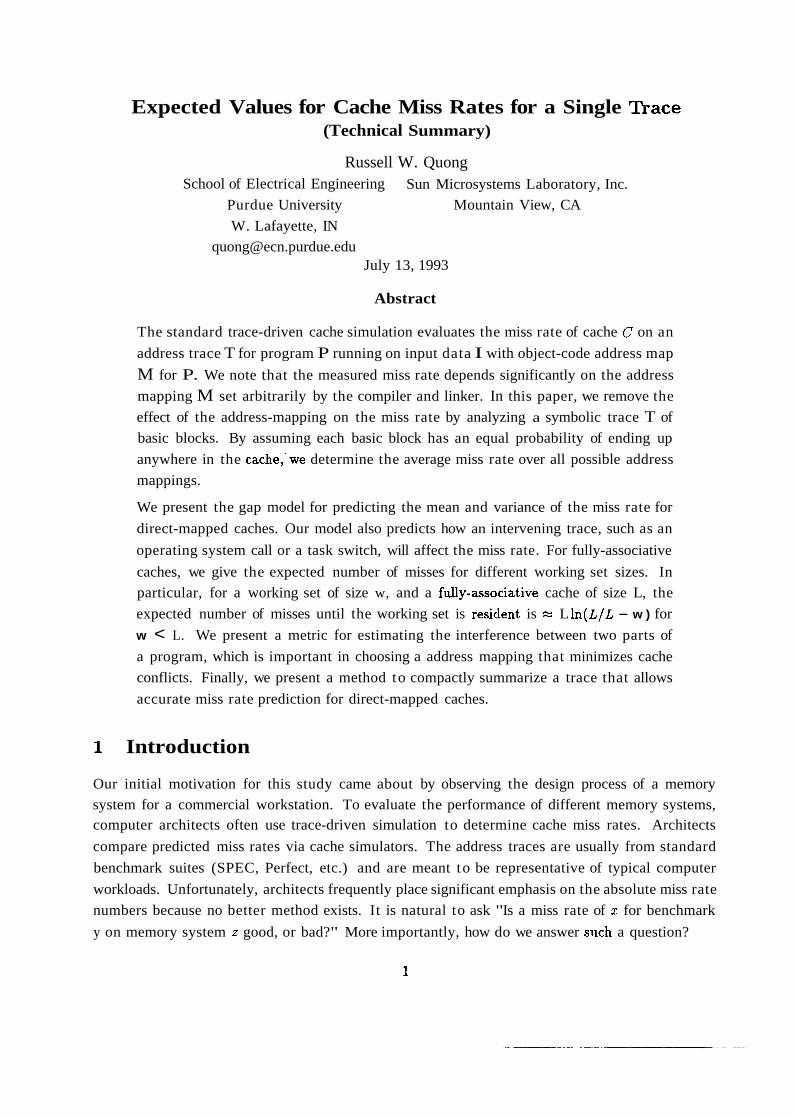
Expected Values for Cache Miss Rates for a Single Dace (Technical Summary)
Russell W. Quong School of Electrical Engineering Sun Microsystems Laboratory, Inc.
Purdue University Mountain View, CA
W. Lafayette, IN
[email protected] July 13, 1993
Abstract
The standard trace-driven cache simulation evaluates the miss rate of cache C on an
address trace T for program P running on input data I with object-code address map
M for P. We note that the measured miss rate depends significantly on the address
mapping M set arbitrarily by the compiler and linker. In this paper, we remove the
effect of the address-mapping on the miss rate by analyzing a symbolic trace T of
basic blocks. By assuming each basic block has an equal probability of ending up
anywhere in the cache,'we determine the average miss rate over all possible address
mappings.
We present the gap model for predicting the mean and variance of the miss rate for
direct-mapped caches. Our model also predicts how an intervening trace, such as an
operating system call or a task switch, will affect the miss rate. For fully-associative
caches, we give the expected number of misses for different working set sizes. In
particular, for a working set of size w, and a fully-associative cache of size L, the
expected number of misses until the working set is resident is = L ln(L/L - w ) for
w < L. We present a metric for estimating the interference between two parts of
a program, which is important in choosing a address mapping that minimizes cache
conflicts. Finally, we present a method to compactly summarize a trace that allows
accurate miss rate prediction for direct-mapped caches.
1 Introduction
Our initial motivation for this study came about by observing the design process of a memory
system for a commercial workstation. To evaluate the performance of different memory systems, computer architects often use trace-driven simulation to determine cache miss rates. Architects
compare predicted miss rates via cache simulators. The address traces are usually from standard
benchmark suites (SPEC, Perfect, etc.) and are meant to be representative of typical computer
workloads. Unfortunately, architects frequently place significant emphasis on the absolute miss rate
numbers because no better method exists. It is natural to ask "Is a miss rate of x for benchmark
y on memory system z good, or bad?" More importantly, how do we answer such a question?

The measured cache miss rate depends on four factors, (i) the program P being executed, (ii) the input data I for P , (iii) the type of cache used, and (iv) the specific address mapping M of
the object code for P, which is determined automatically by the compiler and linker.
We are concerned with the last factor. An address mapping, M, assigns each basic block in
P to a unique set of physical addresses. A mapping is itself affected by many factors including
compiler optimization (such as procedure inlining), the order the object modules are linked, and
the specific libraries on a system. We wondered how much the miss rate would vary if we linked
program b differently?
As such, we question the accuracy of using a single address trace from 'P based on a single
mapping to represent the expected behavior of P, even for similar input data, because of seemingly
arbitrary variations in the address mapping from system to system. We have heard of extreme
stories in which changing the order object modules are linked has changed the execution time by a
factor of two due to caching effects. It is apparent the specific address mapping can have significant
effects on cache performance. In a worse case scenario, the most frequently executed code would
be mapped over one another. Although, such a scenario is unlikely, it is natural to ask how likely
are bad address mappings? In particular, how much variation in miss rate are we likely to observe
simply due to different address mappings?
To isolate the effect of an address mapping from a partic~dar address trace, we view the execution
of P on I as a block trace (or, simply trace) as a sequence of "named" blocks, e.g. "blockl2 of
function sqrt". Thus, for any address mapping M, running program P on input I always produces
the same trace. The advantage of defining traces in this way is that small perturbations to P or I produce small perturbations to the resulting trace. For example, if small changes are made to P
over time, such as fixing bugs or adding new features, we expect the traces from the modified P
and the original P to be roughly the same. The same argument holds true for input I. E.g. if P
is a VLSI layout tool, we would expect similar traces when laying out similar circuits.
Given a block trace, we derive formulas for the expected number of misses averaged over all
possible address mappings of that trace for direct-mapped and fully associative caches. Our method
has the advantage of defining a single meaningful number for the miss rate of a given memory
system for a specific benchmark. Our cache models handle the expected effect on the miss rate of
intervening traces, such as process switches. Finally, our models provide a quantitative measure of
the expected interference in the cache between two parts of a program.
The paper is organized as follows. Section 2 gives states our definitions and assumptions. In
Section 3, we present the gap model and derive equations the mean and variance of the miss rate
for direct-mapped caches. We also show how to model the effect on the miss rate of intervening traces, such as an kernel traps or kernel calls. Finally we describe how to compactly summarize
a trace by giving gap counts. In Section 4, we derive the expected number of misses for a fully
associative cache using random replacement for different working set sizes.

2 Definitions
A cache is described by the triple C(L, LS, SS), where L = the number of lines in the cache, L S = the line size in bytes, and SS = the number of sets or the set size. A cache has SS sets, each of which
contains L I S S lines or slots. For a direct-mapped cache, SS = L; for a fully-associative cache,
SS = 1. Otherwise, we have a a-associative cache, where a = LISS. In this paper, all addresses
and sizes will be measured in units of cache lines, so that the phrase "u unique addresses" means
u unique cache lines. Two addresses collide if they map to the same cache line. We define z = the
probability that two different addresses collide. For a direct-mapped cache, x = 1/L. An address
in the cache is called resident.
We use lower case letters for program-specific values and upper case symbols for trace-specific
values. We denote definitions via italics or with the = symbol. We assume we have a program P whose instruction segment is partitioned into a set of n (basic) blocks B = {I,, . . . b,). A block b is
a segment of machine code such that if one instruction in I is executed, all of b must be executed.
We denote the size of block b; as s;, where s; is the number of cache lines occupied by b;; note that
s; can be fractional. E.g. on a cache with 32-byte lines, a 40-byte block has size 40132 = 514.
We are given a fixed trace, T(P , I ) , for program P running input I. A block trace or tmce T is
sequence of blocks (not addresses) B1, B2,. . ., BN, where B; E B. Because we are interested in the
state of the cache between reference, we view block Bt as being accessed or referenced immediately
after time t. If Bt = b;, then all of block b; is contained in the cache at time t + 1. As our analysis
assumes a fixed trace T , and we omit T when convenient.
Times are denoted by the letter t. A time interval is denotecl [t,tl] where t 5 t'. The term N; denotes the number of times block b; is referenced in T , thus, N = Cr N;. The
term t;(k) represents the time of the k-th reference of block I;. A gap of block b; is the time interval
between references to b;. The first gap of b; is [O,t;(l)], namely, the time interval from startup
to the first reference to b;'. There are N; gaps of b;. We denote the kth gap of b; as [gap;(k)] = [t;(k - 1) + 1, t;(k)]. The length of [gap;(k)] is t;(k) - t;(k - 1).
We define U[tl, t"] = {b;lBtt = b;, t' < tt < t") = the set of nniqne blocks accessed between time
t' and t", not including time t' or t". We denote the size of U[t, t'] as 1 U [t, t'] 1, so that 1 U [t, t'] I is the
number of unique addresses referenced between time t and t'. We define the size of gap [gap;(k)] as
u(i, k) G the number of unique references in the kth gap of I;. Table 1 summarizes the definitions
used in this paper.
As an example, let P consist of basic blocks B = {I1, b2,. . . , Is), where s; = i. Let trace T =
b2, b4, bl, b2, bs, bl, b4, b2. We have B1 = b2, B2 = b4, B3 = 4. The gaps of b2 are [gap2(l)] = [O, I], [gap2(2)] = [2,4], and [gapz(3)] = [5,8]. We have U[2,7] = {11,12,15), IU[2,7]1 = 1 + 2 + 5 = 8, andu(2,3) = IU[5,8]1 = 5 + 1 + 4 = 10.
For any random variable (r.v.) Z, E[Z] 2 = the expected value of Z, and Var[Z] the
variance of Z = E[(Z - z)2]. If Z E { O , l ) ( a Bernoulli trial), then Var[Z] = z ( 1 - 2). We use
'This definition allows us to catch cache misses at startup and also si~nplifies later formulas because there are Ni gaps rather than Ni - 1 which would have resulted if we ignored the first gap.

Table 1: Definitions
Program value
b; block i of program P n number of blocks in P
s; size of block i (in cache lines)
[t, t'] time interval from t to t', t 5 t'
L size of the cache (in lines)
x probability two addresses collide
random variables named S = 1 to represent blocks surviving in the cache, and X = 1 to represent
cache misses.
We make the following assumptions in our analysis.
Trace value
Bt block a.ccessed just after time t
N number of blocks in trace T
Ni # times hi is accessed in T
u(i, k) # unique addr in k-th gap of b; (gap size)
g ( i , k) # addr of k-th gap of b; (gap length)
S(i , t) # of resident addresses of b; at time t
X;(k) # of misses blamed on b; in its kth gap
t;(k) time of k-th reference to block b;
1. For 1 5 i 5 n, s; << ILJ - each block b; is much smaller than the cache, e.g. each block is no
larger than 1/20 of the cache size.
2. JCI >> 1 - the number of cache lines is much greater than 1, e.g. the cache has at least 50
lines.
3. I PI >> ICI - the size of program P is much larger than the cache.
4. Block b; is equally likely to start at any line in the cache. This assumption follows from 3, by
considering all possible address maps of P. (This assumption allows for physically impossible
mappings such as having every block start at line 1 in the cache. It can be proven that
the physicdy impossible mappings are improbable enough to have an insignificant effect on
the final answer. Throughout this paper, we shall assume z the probability that any two
addresses A1 and A2 collide is 1/L. In practice, address mappings are continuous, laying out
blocks one after another, so that
To apply this correction, use the exact value for z wherever the term 1/L is found.
5. Addresses in the same block do not collide with each other except for a fully associative cache
using random replacement.
In practice, these assumptions are usually valid. Note, if blocks are basic blocks in machine
code, the assumptions on block size are quite reasonable.

3 A Gap Model of Direct Mapped Caches
3.1 The expected miss rate
We blame each cache miss on the block currently being accessed, which then replaces a resident
address. We calculate the expected number of cache misses in trace T by adding the expected
number of misses for each block bi over all blocks. To determine the number of misses blamed on
block b;, we consider each of the gaps of b;. The intuitive reason for using gaps is that if Bt = b;,
at t + 1 all of b; must be in the cache, so that the previous status of b; is irrelevant for future times.
We define the random variable
S(i , t) E the number of addresses of b; in the cache at time t.
S( i , t) denotes the number of "survivors" of b; since its last reference. To determine S(i , t) assume
[t, tf] is a gap of block b; and blocks bj , bk, b j are accessed at time t + 1, t + 2, t + 3, respectively as
shown below.
time: t t + l t + 2 t + 3 ... t'
block: b; b j bk b j ... bi
Accessing block bj replaces sj lines in the cache. Over all possible address maps, each line of
b; has a (1 - sj/L) chance of surviving. (This analysis remains true even if part of bj was already
in the cache.) The expected number of cache lines for bi that survive past the reference to b j
is E[S(i, t + 2)] = s;(l - sj/L). Similarly, after referencing bk at t + 2 we have E[S(i, t + 3)] = s;(l - sj/L)(l - sk/L).
However, S(i , t + 4) = S(i, t + 3), because at t + 3 we reference bj which has already been
referenced earlier in this gap. This and subsequent references to bj in this gap cannot replace any
b; lines in the cache, because the first reference to bj would have already done so. Thus, only the
first access t o each block in the gap matters, and we need only consider the set of unique blocks
accessed in [t,t7], namely U[t,t7]. As a result, the expected value of S(i , tf) is
In practice, we will probably need to add a correction factor because blocks that follow one another
in the trace are often "neighboring" blocks in program (e.g. spatial locality). Thus, a significant
number of conflicts from the gap model simply won't occur in practice. The reason is that the
compiler and linker place neighboring blocks at adjacent addresses, with the result that they will
not collide. Our correction consists of labelling pairs of blocks (b;, bj) exempt from colliding with
each other. For example, we might declare all blocks in the same procedure exempt from collisions
with one another, which assumes the cache is larger than any procedure. With exempt pairs, we
modify Equation 1 so that the (1 - se/L) term exists only for non-exempt blocks be of b;.
We define the random variable
X,(k) = s; - S(i, t;(k)) = # of cache misses blamed on b; after its kth gap,

because the number of misses is the block size minurthe number of surviving lines. Summing over
all the gaps of b;, we get the expected number of misses blamed on I; over the entire trace is
The total number of misses over the entire trace is the sum of the misses over all blocks, X(T) =
C?='=, X;. The miss rate is the number of misses divided by the total number of accesses in the trace. If b; is accessed at time t , Bt = b;, then si cache lines are referenced at t.
As a simplification, for L > 1 and L >> s p 2 1, we have (1 - s;/L) x (1 - I/L)" z e - ( ~ ~ / ~ ) .
Thus, applied t o the kth gap of b;, Equation 1 becomes
E[S(i, k)] = si n ( 1 - se/L) x s; n = s;e -u(i, k)/L
4 4 (2)
E[X(i, k)] = 1 - E[S(i, k)] = s; (3)
As an example, Equation 3 shows that if the gap is the same size as the cache, b; has a e-l = 36.8%
chance of surviving. Summing over all gaps of blocks gives the expected number of misses over T.
We grossly categorize gaps sizes as either small (survival is likely), mediiim (survival depends on the
specific address map) or large (survival unlikely). For small gap sizes u. less than L/4, the chance
of surviving is sz (1 - u/L). For gaps larger than 3L, b; has less than a 5% chance of surviving,
indicating b; is almost always knocked out. Thus, for any address mapping, blocks will survive
small gaps and will not survive large gaps. Alternatively phrased, for a specific address mapping,
the main factor of the actual cache performance is the miss rate on mid-sized gaps, e.g. those with
sizes between L/30-3L.
Note that our model provides quantitative insight on how much each block accounts for cache
misses. Unlike other miss rate models, Equation 4 is a weighted sum of exponentials. With different
weights, Equation 4 accounts for a wide variety of miss-rate versus caches size behaviors.
3.2 Data Caches
The preceding analysis assumes only instruction address traces. We now discuss data-only caches
and then mixed caches. When considering data references, some of our previous assumptions no
longer apply. We make the following modifications to our model. Data consists of either scalars or
arrays. In general, a trace consists of a series of blocks and array references B1, Bp, . . . , B;, . . . , BN,
where B; is either a basic block, a scalar, or an index from an array, such as "index 42 from array
17." As before, we assume the sizes of all blocks, scalars, and arrays are known.

Each scalar is treated as a block, except that scalars have fractional sizes. E.g. on a cache with 32-byte lines, a $-byte integer scalar has size 4/32 = 118. Allowing fractional sizes is a better
model for blocks/scalars that are likely to be in the same cache line, because in Equation 1, we are
interested in the number of unique cache lines used. Rounding sizes up to the nearest integer is
a better model for blocks that are unlikely to occupy the same line, such as when text and data
collide in a mixed cache. As a contrived example, if eight scalars fit in a cache line, and L = 128,
what is the likelihood that a scalar will survive through a gap that references 128 other scalars?
We believe spatial locality implies that if two scalars are accessed close to each other in time (such
as local variables for a given function), they are likely to be close to each other in the address map,
perhaps in the same line.
Arrays however, do not fit perfectly into the block model. Like basic blocks, arrays occupy
contiguous addresses, and thus, array addresses do not collide with one another (unless the arra.y
is larger than the cache). Unlike blocks, however, (i) arrays can be quite large relative to the cache
size, and (ii) arrays need not be referenced in their entirety. We model small arrays as blocks that
need not be referenced in their entirety.
We categorize arrays as either small or large. If an array A[] is small, say IAJ < L/5, we treat
each entry of A as a separate scalar. Otherwise, if an array A[] is large, we cannot use our previol~s
approximation. We define S(i , A[], T) the expected number of addresses of block b; that survive
T unique references to A[]. We have S(i, A[], T) = (1 - rsA/L), where s~ is the size (in cache lines)
of an array element. If the array is accessed sequentially, i.e. via indices 5, 6, 7, 8 . . . , then s~ is
the fractional size of each array element. Thus, if an array is one-third of the size of the cache and
it is accessed in its entirety, then TSA = L/3 and the pro1,ability of an address surviving is 213,
which is what we would expect.
Thus, we amend the Equation 1 on the expected number of lines of bi that survive through time
t' to be
be E U[t, t'], A,[] E U[t, t'],
where each bc is a block or scalar, and each A, is a large array of with elements of size s ~ , to which
there are TK unique references during [t, t'].
3.3 Mixed instruction and data caches
Although not obvious, the equations for instruction-only caches remain reasonably accurate for
traces with both instruction and data addresses. We can still use the approximations from Equa.-
tion 2 because if (for a large array) TSA is large relative to the cache size (say, 2 L/5), the gap size
must also be large, as instruction references must outnumbel. array references. The inaccuracy of
the approximation (1 - s/L) = e-'IL only matters when L/5 < rsa 5 L. If TSA > L, the term
e-~(',k)/L = o which remains accurate. ~f TSA is small relative to L, our approximation
is obviously valid. Thus, for the kth gap of b;, Equations 2 and 3 remain

E[S(i, k)] = k)/L
E[X(i, k)] = 1 - :E[S(i, k)] = s;
where u(i, k) now counts all unique addresses including array references.
3.4 The interference between blocks
We can now quantitatively define the interference between two blocks blocks b; and bj. We define
two random variables Y(i, j, k) and Y(i, j, T ) = the number of cache misses blamed on b; when
referencing bj ( i ) in the k-th gap of bi and (ii) over the entire trace T , respectively. As before,
we sum Y(i, j, k) for each gap of b; to get Y(i, j, T). If [t,t1] is the k-th gap of b; and t j is the
first reference of 6, in the gap, then E[Y(i, j , k)] = S(i , t j ) ( l - sjp) zi s;(l - e-Iu[t~tj+lII/L). The
interference between b; and bj is Z(i : j ) = Y(i, j, T ) + Y(j, i, T) , which gives the desired symmetric
property Z(i : j) = Z ( j : i).
As a generalization of Equation 4, we introduce the interference function
which describes, in theory, the expected miss rate of T for a direct-mapped cache of any size.
3.5 Intervening traces
When analyzing trace T , we define an intervening trace T' as a continlious sequence of blocks during
T that have no addresses in common with T. Thus, we can view (i) operating system calls, (ii)
operating system interrupts and (iii) process switches due to multi-tasking, all as intervening traces.
For simplicity, we assume the intervening trace T' runs to completion without being interrupted
itself. The notation T < T' > indicates that T' was an intervening trace sometime during T.
If T' has U' unique addresses, it increases the size of all pending gaps by U'. An intervening trace
interrupts L gaps. Let G = the sum of all gap lengths. If no information is known a priori as to when
the intervening trace will occur in T , e.g. a hardware timer interrupt, the probability of interrupting
any gap g is proportional to the length of g, Pr[interrupting gap g ] = (length of g) * LIG. For the
kth gap of b;, we define the r.v.
&(k, TI) X;(k,T < T' >) - X;(k,T) = # extra cache misses in kth gap of b; due to T'.
Then the expected value of K(k) is
E[K(k)] = (g(i, ~ ) L / G ) si(e(u(i7 k)+u')/L - 'XL)
The expected number of additional misses due to T' is the sum of E[V,(k)] over aJl gaps.

3.6 An approximate lower bound of misses
Because Equation 4 represents the average number of cache misses for T over all address mappings,
there must exist "good" mappings that result in fewer misses. How well might a good address
mapping perform? Unfortunately, determining the miss rate of the optimal mapping is an NP-hard
problem. However, using the gap model we can estimate a lower bound.
As done in [McF89], we use the optimal cache-line replacement strategy, OPT, to derive a lower
bound. On a cache miss, OPT replaces the line that will be accessed furthest into the future.
Although OPT is impossible t o implement in practice (as it requires knowledge of the future and
a fully associative cache to boot), the miss rate of OPT forms a convenient comparison point. We
can overestimate the number of misses for OPT, by discarding all terms in Equation 4 for gaps of
size less than L, as seen by following lemma.
Lemma 1 If block b; has a gap g of size u, using the OPT replacement strategy, b; survives through
g i f s ; + u < L.
Proof: Let U be the set of addresses referenced in gap y. Assume g starts a t time t . Rank
(with labels 1, 2,3, . . . , L) each of the addresses resident a t t based on the time of the next access,
with lower ranks for sooner accesses. Let r be the number of a~ldresses in U are already resident
and x = u - T of the addresses are not resident a t t. At the end of g, OPT will have replaced the x addresses of largest rank; thus, the L - s addresses with lowest rank must survive through
g. The last address of b; (the address of b; with highest rank) has rank r + s;. From the lemma,
s; + u = s; + x + T < L. Thus, s; + T < - L - x, and b; has low enough rank to survive through g.
We note a block can survive gaps with size greater than L, if OPT replaces parts of U as the
gap progresses. As an example, assume L = 2, and all blocks have size of one. In the following
trace, block bl survives the entire trace including two large gaps.
bl,b2, b3,bl, b4,b5,b6,b7,bl,b2,b3,bl-
3.7 The image of a trace
In this section, we describe methods to compactly summarize the gaps in a trace. Our idea is to
categorize each gap a s either "short" or "longn depending on whether the size of the gap (number
of unique addresses in the gap) is smaller-than, equal-to or larger-than the cache size, L.
Equation 4 shows that the ratio of the gap size to L determines the miss rate. For example, if
the gap size is 5L, then the block probably will not survive the gap as e-5 < .7%. Thus, for each
block, if we know how many gaps are of each size, we can calculate Equation 4 precisely. However,
this information potentially requires keeping information about many gaps sizes.
Instead, we adjust all gap sizes by rounding them to the nearest power of 2, and we count the
number of gaps of each adjusted sizes. For a trace of length N , there are logz N adjusted gap sizes.
Thus, we need loga N integers for each block, or nlog, N integers in total to summarize a trace.
As we alluded earlier, we can group large gaps with sizes 2 5L together. As it is seems unlikely we

will see caches with more than 2 x lo5 cache lines (not bytes) in the near future, in practice, we can lump together all gaps of size greater than lo6. Thus, we need only log2 lo6 x 30 adjusted gap
sizes, meaning we need only (30n) integers to summarize the trace. For example, if N = lo9 and
n = lo4, we need 30 x lo4 = 3 x lo5 integers, a space reduction by a factor of 3 x lo3. Furthermore,
if many blocks have gap sizes with zero counts, we can save more space by listing just the non-zero
entries for each block (analogous t o an adjacency list for representing sparse graphs). This method
could reduce the space needed by another factor of 2-1000 times.
If handling intervening traces is important, we need to store both the length and size of each
gap. As before we can adjust each gap length by rounding to the nearest power of 2, so that we
need n(logz N)z integers. As before, if many entries are zero, we can list just the non-zero entries.
If is not important t o know which blocks are causing the misses, we can lump all blocks together
and simply count adjusted gap sizes weighted by block sizes. That is, if block bi has a gap with
adjusted size 29, then we add s; to the gap count for size 29. In this manner, only log, N integers
are needed. As this is a t most 40 integers in practice, for better accnracy, we might round gap sizes
t o the nearest power of f i or even fl, which would double or qna.<lruple the space requirement.
To capture how the miss rates changes as the trace progresses, we can split T into shorter pieces
and summarize the pieces individually. Finally, we note that our gap model expands upon the LRU stack model of an address trace [Spi77]
[RS77]. In their model, they record the probability that the next address in the trace will be the
mth most recent address. This corresponds to a gap of size m in our model. However, our derivation
points out the expected effect on the miss rate of such an occnrrence.
3.8 Bounds on the variance of X ( T )
Determining the variance of X(T) directly is difficlllt because the terms Xi(k) are not independent.
Although we can derive an analytic formula for Var[X(T)], directly evaluating this formula is
computationally intractable as it involves many, many terms (typically, >> lo8), forcing us t o settle
for bounding the value of Var[X(T)].
Before getting involved in the mathematics, recall the goal of this section is to estimate how
much the miss rate varies. We shall use the variance as a yardstick. However, as we can only
estimate the variance, our methods are approximate at best. As such, we shall sacrifice accuracy
and rigor for simplicity and intuition when possible. For any r.v. X = XI + X2 + . . . + Xn, we have
= sum of variances + cross terms

n
Var[X] > CVar[X;], cross terms 2 0 i=l
If the X; terms are pairwise independent (namely, E[XiXj] = E[Xi]E[Xj]) then the double sum of
cross terms is zero. In our case, Xi and X j represent the number of cache misses when accessing
blocks b; and bj a t times t; and t j , respectively. Unfortnnately, these cross terms are dependent
and there are O(n2) of them. Directly calculating each of these terms is somewhat involved.
Consequently, we shall instead derive upper and lower bounds of Var[X].
The cross terms X;, X j are positively correlated if E[(X; - x;)(x~ - x j ) ] > 0 or alternatively,
E[X;X,] > E[X;]E[Xj]. In this case, Equation 12 shows we can underestimate Var[X] by summing
the variances of the individual Xi. Informally, if knowing that Xi is greater than its average vahie
means that we expect X j to be greater than its average value, then we shall consider X; and X j
to be positively correlated. We believe the sum of cross terms is positive so that discarding them
gives a lower bound.
Both loop iterations are gaps of b;. If we know that bj or bk collide with b; then the X;(k;)
and X;(ki) terms will both have larger than average vdnes, showing they are dependent. We can
also, view the same references in terms of gaps of bj. Here, we see b; and bk in the bj gaps. Thus,
the corresponding Xj(kj) and Xj(ki) terms are related. Finally, the X;(k;) and Xj(kj) terms are
dependent because if b; and bj collide, then both terms will tend to be larger. (All four terms
are dependent, in fact.) Overall, we expect the terms for the same block to be related for this
reason and many of the terms for different blocks to be dependent if references to these blocks are
interleaved as in major loop calls.
We may discard terms for gaps with 2 10L unique addresses because it is unlikely (prob
< 5 x a block can survive the gap. The term E[(X - x)] will be quite small.
We can underestimate Var[X;(k)] by considering each address in a block, independently. We
define the r.v. XiH(k) = 1 if and only the j t h address in L; causes a miss at the end of the kth
gap. Using Equation 3 with s; = 1, gives the value of Xibl(k) = 1. We know X;bl(k) and Xili,](k)
are positively correlated, because if the j th address of b; is replaced dnring the gap, it is likely the
j'th address was also replaced. Thus,
which plugged into Equation 12 gives
We can get a crude estimate of the variance by considering the dominant loops in the trace, as a
significant fraction of the execution trace will consist of iterations from a few major loops. Loop
iterations will appear as consecutive (nearly) identical gaps. In practice, caches are much larger
than a loop body, so that we expect the loop to survive intact from iteration to iteration. Thus,

much of the variance will come from the case where two (or more) blocks collide in a frequently
executed loop. E.g. the gap model predicts no collisions but some occur. In the following, we
assume that dominant loops have been identified by some means.
time: t t + l t + 2 t + 3 ... t'
block: bi b i bk bl ... bi
Consider a loop that is a gap of b; which contains bj once, as shown above. (If a gap contains
more than one occurrence of bj, we consider only the first.) We restrict ourselves to the case where
bi and bj collide. Let X; and X j represent the number of misses on the second loop iteration when
accessing b; and bj. We shall evaluate the cross term in Equation 11, XiXj - XiXj. For simplicity,
we assume the gap size is less than L/10 so that we can ignore the product of the means because
x;xj < el/loel/lo < .O1 x 0. Without loss of generality, if s; 2 sj, there are three cases for bi and
bj: no collision, partial collision, and full collision where b; completely "covers" bj.
sj-1 E[XiXj] = ' [(i - S; - sj + l)(O * 0) + 2 (k * k) + (si - Sj + l ) ( s j * sj)
L k= l I
= no collision + partial collision + full collision
The above cross term applies to each Xi and independently to each X j from each loop iteration.
Thus, if there are m iterations of a particular loop, there a e m2 identical X; X j terms for each i
and j due to the cross product of m Xi terms and m Xj terms. We calclilate similar terms for all pairs of variables involved in the loop. Finally, we apply these terms over all major loops of the
program. Formally, let 4 represent a loop from T that makes 141 iterations. Let i, j E 4 mean that
blocks b; and bj are referenced in each iteration of 4. Then using Eqnation 13, the sum of the loop
cross terms is
4 A fully associative cache
We now consider the expected number of misses for a fully associative cache using random replace-
ment. With this scheme, a random line is replaced on a cache miss. The use of random replacement simplifies our analysis because block collisions are independent of the address mapping. A fully
associative cache dynamically adapts to the trace, so that recently accessed lines are likely to be
in the cache, independent of the trace. We shall use a working-set model [Den681 not the gap
model. Previous studies [Smi78] have shown that fully associative caches have significantly lower

miss rates than direct-mapped caches. The results of this section also apply to a-way set-associative
caches for a 2 4. In practice, a-way set-associative caches, for a 2 4 have similar performance to
fully associative caches. However, full associativity is significantly easier to analyze than a-way
set-associativity.
To analyze a fully associative cache, we consider each a.cl<lress of P individually, because any
address can collide with any other address. In this case, we partition P into n addresses (not
blocks), bl, b2,. . . , b,, where each b; is a cache line's worth of object code.
To gain some insight into how the behavior of a direct-mapped cache differs from that of a fully
associative cache, we shall analyze the expected number of misses for a cyclic trace of w different
addresses bl, bz, . . . , b,-l, b,, bl, b2, . . . , bw-l, b,, bl, . . . on an initially empty cache. Here, w is
meant t o represent the effective working set size. We call 11, 12 , . . . , lw-l,Iw a cycle. Intuitively, if
w 5 L, we expect all addresses will eventually reside in the cache; if w > L, the trace cannot fit in
the cache and at least w - L blocks must miss each cycle.
In a direct-mapped cache, two blocks I; and bj either always conflict or never conflict. Thus,
the expected miss rate from these blocks over all mappings is 1/L for each reference. In contrast,
on a fully associative cache, bl and b2 will probably be placed in different cache locations initially
resulting in no further collisions. However, there is a chance L1 and lz might collide one or more
times before both become resident.
4.1 Small working sets, w 5 L
We now solve for the expected number of misses when dealing with an arbitrary trace of w distinct
addresses where w 5 L. We shall categorize the state of the cache by u, the number of unique
addresses it contains. Note that u must monotonically increase, becanse on a cache miss, we either
replace an old address leaving u unchanged, or we load the new address into an empty cache line
incrementing u. Once u = w, there will be no further misses.
Let X ( n + n + 1) = the expected number of misses starting with u = n until u = n + 1. For
example, a[0 + 11 = 1, as the first access misses and becomes resiclent. However, if w = L and
u = w - 1, t o increment u t o w requires filling the one empty line rather than replacing any of the
L - 1 resident addresses on a miss. As we shall see, ~ [ n + n + 11 = L/(L - n), so that X[L- 1 4 L] . = L misses are needed on average t o randomly fill the last slot. Note that we ignore cache hits at
this point, and it will be the case that many hits occur between misses. We have

Table 2: Total misses for w = aL , as a ratio of compulsory misses
- a = w/L
misses: total/compulsory
We have Pr[ X ( n -+ n + 1) 2 i ] = ( n / ~ ) ~ - ' because we need ( i - 1) consecutive misses that replace
one of the n resident addresses in the cache. In general ~ ( a -+ b) = c::' ~ ( n -+ n + 1). Using
Hn = C7=l l/i = In n + .577 + 1/(2n) - 1/(12n2) [GKP89],
L - a = L l n - ( I - a) [ L - b + 2(L - a)(L - b) I
.1
1.05
Thus, if a = 0 and b = L, we expect = L In L misses from Equation 15. Alternatively, if a = 0
and b = w = aL, each address has ( l / a ) ( ln ( l / l - a ) misses on average. Table 2 shows that
for w < 50%L, compulsory misses account for most of the misses, indicating that cache quickly
captures the working set if the working set is smaller than the cache. In practice, caches will
frequently be much larger than the working set, so that r~ << 1. For a << 1, use of the Taylor
expansion ln(1 + x) = x - x2/2 + . . ., for 0 < x << 1, shows that the ratio of total misses over
compulsory misses is roughly 1 + a/2(1 - a) .
.25
1.15
The preceding analysis only considers cache misses. We now calculate the expected number of
.66 1.63
total references, including cache hits, for the working set to become resident, assuming addresses
.33
1.21
are accessed randomly from the w addresses in the working set. Let R(a -+ b) = the expected
number of references starting with u = a until u = b and let a ( a ) be the expected number of
.50
1.39
.75
1.85
references until a cache miss occurs if there are a resident a.ddresses in the cache.
We have Pr[ Q(a) 2 i ] = ( ~ / w ) ~ - l because we need i - 1 consecutive references to one of the a
resident addresses in the cache, giving i - 1 consecutive cache hits. Combining this result with
Equation 14 gives
.80
2.01
.90
2.56

In most cases, b = w as we assume the entire working set becomes resident. In particular, if a = 0 and b = w = L - 1 , there are (L - I)* references on average before the working set is resident. If
w = crL, where cr << 1, then R ( O -+ w) % (w/(l - a))ln(w(l - a)) .
The above analysis makes the implicit assumption that every block in the working set is accessed
regularly, such as a cyclic trace, so that the entire working set eventllally becomes resident. In
practice, traces will rarely be so cooperative. To handle irregular access to the working set, we
shall augment T with extra references.
We prove that adding blocks to a trace cannot decrease the expected number of misses. (Note,
this process may decrease the miss rate, as the trace becomes longer.) We denote an insertion
as insert(T, b,, t) = add a reference t o b, to T immediately after Bt before Bt+1. Thus, if T =
B1, . . . , Bt , Bt+l, . . . , BN, then insert(T, b,, t ) = B1, . . . , Bt , b,, Bt+1, BN. As before X(T) is the expected number of misses on trace T.
Lemma 2 For any trace T, let T' = insert(T, b,, t). Then, x ( T ) <_ X(T1).
Proof: There are two cases.
(i) Block b, is present in the cache at time t. The extra reference to b, is a cache hit so
X(T) = X(T').
(ii) Block b, replaces block b, a t time t in the cache. We consider the misses blamed on b, and
b, - Misses blamed on b, - In trace T, if I, survives until its next reference, we get an extra miss
in TI on the next reference to b,. If b, wollld have been replaced anyways before its next
reference, the extra b, causes no change. In both cases, we have X(T) < x(T').
Misses blamed on b, - In T', the extra b, either prefetches b, if b, survives until its next
reference or generates an extra miss if I, is replaced by its next reference. In either case,
X(T) 5 X(T'). a
L-1 00
' I f a = 0 , and b = 4 = L, we get R(0 - L) = L2/(L - i)2 s LZx2/6 = 11.6L2. We have used l/i2 = r2/6. i = O i = l

Theorem 1 For any tmce T, let T2 be the resulting truce ufter un arbitrury number of insertions
on T. Then, 8 ( ~ ) 5 x(T~).
Proof: By repeated single insertions we can convert T to T2. The theorem follows by repeated
application of the lemma.
We use this theorem to get bounds on the misses for traces with irregular reference patterns.
For example, let b4 represent the blocks in a loop body and consider the trace (fragment) To = b,, b2, bd, bd, b,, bl, b2, bd, bd, bz, bd, bd in which bl and b2 are accessed sporadically. At the end of
To, it is not clear whether bl is likely to be resident, because the last reference to bl occur By
inserting references to bl and bz before bd when necessary, we can convert To to TA, a sequence
of cyclic traces so that Equation 15 applies. If w for To is small and the cache is initially empty,
we get the bounds w 5 X(TO) 5 X(T:) = Lln(L/L - w). For w < L/10, Table 2 shows that
w = Lh(L /L - w), indicating our bounds are quite tight. Other trace fragments can be handled
similarly.
4.2 Analyzing the trace, w 5 L
To determine the expected number of misses on T, we assume the T has been partitioned by some
means into sub-traces TI,. . . , TN, such that each sub-traces has a different working set than its
neighbors. E.g each time the working set changes, we get a new working set. The working set for
Tt is Wt; its size (in cache lines) is wt. We assume wt 5 L, and that after each subtrace, the entire
working set W; is resident. In this section (Section 4.2), we clenote the time immediately before
subtrace Tt as time t, e.g. it is as if each subtrace requires one unit of time. The notation bj E Wt
means that address bj is part of working set Wt.
Within each subtrace Tt, we have X ( T ~ ) = X(at -t wt), where ut is the expected number of
addresses of Wi already resident a t the start of Tt. We use the gap moclel to determine at. We
define the random variables
1 b; in the cache at time t S(i, t ) =
0 bi not in the cache a.t time t '
and
S(W;,t) = S(j , t). bjEWi
Thus, S(W;,t) is the number of addresses of W; that are resiclent a t time t. Let b; E Wt as
shown below. The probability that address b; will survive through subtrace Tt+1 is (1 - wt+l/L),
assuming none of Wt+1 was resident before However, if a r u t + l addresses of Wt+1 survived
from a previous subtrace through Tt, then during Tt+1 only (1 - a)wt+1 addresses will be reloaded
into the cache, and the probability of b; surviving though Tt+l is (1 - (1 - cr)wt+l/L).
time: t t + l blocks: . . .bi ... bjl b j2 . . . b jn - - .
subtrace: I t T t - t I I + Tt+l - I

Thus, the number of addresses of Wt already resident before Tt is ut = S(wt, t), which is defined
by the recurrences
E[S(i , t + l ) ] = 1, bi E Wt
E[S(j, t + I)] = E[S(j, t + 1)] * (1 - L
As an example, consider the case where two working sets, Wt and Wt+1 overlap in their transition.
We model the overlap in a separate subtrace that references the large working set Wt U Wt+1 that has
been warm-started with all of Wt resident. Then during the transition, we expect x ( w l -+ wl +w2)
= L ln misses from Equation 16. After the transition, Wt+1 is already resident and no -(Y +w )
further misses are encountered.
4.3 Working sets larger than the cache, w > L
[Originally we tried t o analyze fully-associative caches using the following analysis, however it yields
erroneous results when w 5 L. Fortunately, it yields reasonably accurate results for w > L. In
practice, caches are becoming large enough so that w > L is increasingly unlikely.] If w >> L (say w > 5L), we can again apply the gap model, because few addresses will survive
their gaps. In particular, an address will survive with probd~ility e-'"IL, giving a miss rate of
1 - e-WIL. (A brief simulation indicates this model is quite accurate for w 2 3L.) The probability
of a miss when accessing bi at time t depends in part on the likelihood of b; already residing in the
cache. As before, we define the random variable
1 b; in the cache a t time t S(i, t ) = {
0 b; not in the cache a t time t
If w >> L, the probability of an address surviving through a cycle until its next reference is small,
and we may assume with little loss in accuracy that S( i , t ) is independent of S ( j , t ) for any i and
j. Then, if Bt = b;, we have
1 - E[S(i, t)] E[S(j, t + I)] = E[S(j, t)] * (1 - L 1
L - 1 + E[S(i, t)] = E[S(j, t)l * ( L 1 i # j
In Equation 23, the term (1 - E[S(i, t]) is the probability that b; is not in the cache and the term
(1 - E[S( i , t ) ] ) l~ is the probability bi replaces bj in the cache. For the cyclic trace, we assume the
cache reaches a stationary state in which S( j , t ) depends only on how long ago b, was referenced,
and we can treat all blocks identically, except they are shifted in time. We define S( t ) = expected
value of S( j , t) where bj was referenced t time units ago. In the cyclic trace, each address has a ga.p

Table 3: Comparison of predicted and measured miss rates for L = 32 on a cyclic trace of zu
addresses.
of length w - 1, so the currently referenced address has probability S(ru - 1) of still being resident
in the cache. Using Equations 22 and 23, we can solve for S(ru - 1).
w
calculatedx
measured
w
calculatedx
measured
w
calculatedx
measured
Taking the logarithm of Equation 25 and rearranging gives a transcendental equation which defines
the expected miss rate, X, which is 1 - S(TU - 1).
After solving for X iteratively, Table 3 shows that the calculated miss rate from Equation 26
matches well with simulation results for w 2 1.5L. For Table 3, we measured the miss rate of a
fully associative cache on 100 cycles of the trace 1,2,3,. . . , w. Because random replacement is used,
we can only calculate the expected miss rate. In We chose L = 32 in Table 3, because in practice,
TLB's are often fully associative and TLB's are frequently of this size.
32
0.0%
- % 64
79.0%
79.8%
96
94.0% 94.1%
4.4 Intervening traces
Assume at some point during trace T the working set size is w and u of these addresses are
resident. If an intervening trace T' occurs with u' unique a.~ldresses that all become resident, it
reduces the expected number of resident addresses of T to u(1 - ul/L), using the same reasoning
as for Equation 1. After T' ends, we expect x [ u ( l - ul/L) + IU] more misses until the working set
from T become fully resident.
36
16.9%
23.6%
68
82.3%
83.0%
100
94.9% 95.0%
40
33.7%
38.8%
72
85.0%
85.5%
104
95.5%
95.6%
44
46.6%
50.3%
76
87.1%
87.7%
108
96.1% 96.2%
48
56.2%
58.9%
80
88.9%
89.5%
112
96.7% 96.7%
52
64.0%
66.0%
84
90.7%
91.0%
116
97.0% 97.1%
56
70.0%
71.7%
88
91.9%
92.4%
120
97.6% 97.5%
6 0
75.1%
76.4%
92
93.1%
93.3%
124
97.9%
97.8%
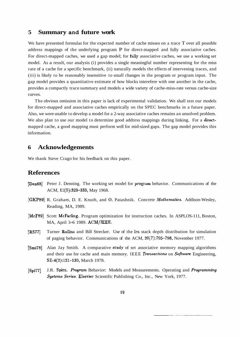
5 Summary and future work
We have presented formulas for the expected number of cache misses on a trace T over all possible
address mappings of the underlying program P for direct-mapped and fully associative caches.
For direct-mapped caches, we used a gap model; for fully associative caches, we use a working set
model. As a result, our analysis (i) provides a single meaningful number representing for the miss
rate of a cache for a specific benchmark, (ii) naturally models the effects of intervening traces, and
(iii) is likely to be reasonably insensitive to small changes in the program or program input. The
gap model provides a quantitative estimate of how blocks interefere with one another in the cache,
provides a compactly trace summary and models a wide variety of cache-miss-rate versus cache-size
curves.
The obvious omission in this paper is lack of experimental validation. We shall test our models
for direct-mapped and associative caches empirically on the SPEC benchmarks in a future paper.
Also, we were unable to develop a model for a 2-way associative caches remains an unsolved problem.
We also plan to use our model to determine good address mappings during linking. For a direct-
mapped cache, a good mapping must perform well for mid-sized gaps. The gap model provides this
information.
6 Acknowledgements
We thank Steve Crago for his feedback on this paper.
References
[Den681 Peter J. Denning. The working set model for program behavior. Communications of the
ACM, 11(5):323-333, May 1968.
[GKP89] R. Graham, D. E. Knuth, and 0. Patashnik. Concrete M(1thematics. Addison-Wesley,
Reading, MA, 1989.
[McF89] Scott McFarling. Program optimization for instruction caches. In ASPLOS-111, Boston,
MA, April 3-6 1989. ACMIIEEE.
[RS77] Turner Rollins and Bill Strecker. Use of the lrll stack depth distribution for simulation
of paging behavior. Communications of the ACM, 20(7):795-798, November 1977.
[Smi78] Alan Jay Smith. A comparative stl~dy of set associative memory mapping algorithms
and their use for cache and main memory. IEEE Trunsuctions on Software Engineering,
SE-4(2):121-130, March 1978.
[Spi77] J.R. Spirn. Program Behavior: Models and Measurements. Operating and Progrumming
Systems Series. Elsevier Scientific Publishing Co., Inc., New York, 1977.