Expected Eligibility Traces

Hado van Hasselt1 , Sephora Madjiheurem2 , Matteo Hessel1

David Silver1 , Andre Barreto1 , Diana Borsa1

1 DeepMind2 University College London, UK

Abstract

The question of how to determine which states and actionsare responsible for a certain outcome is known as the creditassignment problem and remains a central research questionin reinforcement learning and artificial intelligence. Eligibil-ity traces enable efficient credit assignment to the recent se-quence of states and actions experienced by the agent, but notto counterfactual sequences that could also have led to thecurrent state. In this work, we introduce expected eligibilitytraces. Expected traces allow, with a single update, to updatestates and actions that could have preceded the current state,even if they did not do so on this occasion. We discuss whenexpected traces provide benefits over classic (instantaneous)traces in temporal-difference learning, and show that some-times substantial improvements can be attained. We providea way to smoothly interpolate between instantaneous and ex-pected traces by a mechanism similar to bootstrapping, whichensures that the resulting algorithm is a strict generalisationof TD(λ). Finally, we discuss possible extensions and connec-tions to related ideas, such as successor features.

Appropriate credit assignment has long been a major re-search topic in artificial intelligence (Minsky 1963). To makeeffective decisions and understand the world, we need toaccurately associate events, like rewards or penalties, to rele-vant earlier decisions or situations. This is important both forlearning accurate predictions, and for making good decisions.

Temporal credit assignment can be achieved with repeatedtemporal-difference (TD) updates (Sutton 1988). One-stepTD updates propagate information slowly: when a surpris-ing value is observed, the state immediately preceding it isupdated, but no earlier states or decisions are updated. Multi-step updates (Sutton 1988; Sutton and Barto 2018) propagateinformation faster over longer temporal spans, speeding upcredit assignment and learning. Multi-step updates can beimplemented online using eligibility traces (Sutton 1988),without incurring significant additional computational ex-pense, even if the time spans are long; these algorithms havecomputation that is independent of the temporal span of theprediction (van Hasselt and Sutton 2015).

Traces provide temporal credit assignment, but do not as-sign credit counterfactually to states or actions that couldhave led to the current state, but did not do so this time.

Copyright © 2021, Association for the Advancement of ArtificialIntelligence (www.aaai.org). All rights reserved.

MDP True value TD(0) TD( ) ET( )

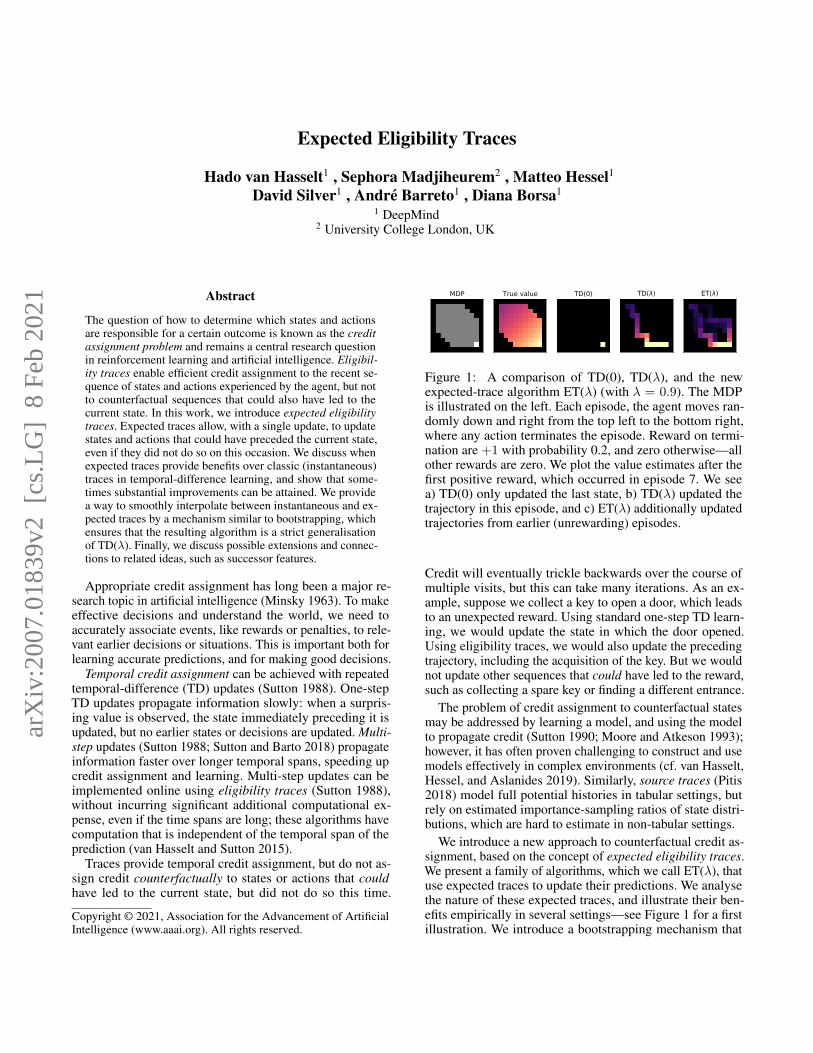
Figure 1: A comparison of TD(0), TD(λ), and the newexpected-trace algorithm ET(λ) (with λ = 0.9). The MDPis illustrated on the left. Each episode, the agent moves ran-domly down and right from the top left to the bottom right,where any action terminates the episode. Reward on termi-nation are +1 with probability 0.2, and zero otherwise—allother rewards are zero. We plot the value estimates after thefirst positive reward, which occurred in episode 7. We seea) TD(0) only updated the last state, b) TD(λ) updated thetrajectory in this episode, and c) ET(λ) additionally updatedtrajectories from earlier (unrewarding) episodes.

Credit will eventually trickle backwards over the course ofmultiple visits, but this can take many iterations. As an ex-ample, suppose we collect a key to open a door, which leadsto an unexpected reward. Using standard one-step TD learn-ing, we would update the state in which the door opened.Using eligibility traces, we would also update the precedingtrajectory, including the acquisition of the key. But we wouldnot update other sequences that could have led to the reward,such as collecting a spare key or finding a different entrance.

The problem of credit assignment to counterfactual statesmay be addressed by learning a model, and using the modelto propagate credit (Sutton 1990; Moore and Atkeson 1993);however, it has often proven challenging to construct and usemodels effectively in complex environments (cf. van Hasselt,Hessel, and Aslanides 2019). Similarly, source traces (Pitis2018) model full potential histories in tabular settings, butrely on estimated importance-sampling ratios of state distri-butions, which are hard to estimate in non-tabular settings.

We introduce a new approach to counterfactual credit as-signment, based on the concept of expected eligibility traces.We present a family of algorithms, which we call ET(λ), thatuse expected traces to update their predictions. We analysethe nature of these expected traces, and illustrate their ben-efits empirically in several settings—see Figure 1 for a firstillustration. We introduce a bootstrapping mechanism that

arX

iv:2

007.

0183

9v2

[cs

.LG

] 8

Feb

202

1

provides a spectrum of algorithms between standard eligi-bility traces and expected eligibility traces, and also discussways to apply these ideas with deep neural networks. Finally,we discuss possible extensions and connections to relatedideas such as successor features.

BackgroundSequential decision problems can be modelled as Markovdecision processes1 (MDP) (S,A, p) (Puterman 1994), withstate space S, action space A, and a joint transition andreward distribution p(r, s′|s, a). An agent selects actions ac-cording to its policy π, such that At ∼ π(·|St) where π(a|s)denotes the probability of selecting a in s, and observes ran-dom rewards and states generated according to the MDP, re-sulting in trajectories τt:T = {St, At, Rt+1, St+1, . . . , ST }.A central goal is to predict returns of future discounted re-wards (Sutton and Barto 2018)

Gt ≡ G(τt:T ) = Rt+1 + γt+1Rt+2 + γt+1γt+2Rt+3 + . . .

=T∑i=1

γ(i−1)t+i Rt+i ,

where T is for instance the time the current episode termi-nates or T = ∞, and where γt ∈ [0, 1] is a (possibly con-stant) discount factor and γ

(i)t =

∏ik=1 γt+k. The value

vπ(s) = E [Gt|St = s, π ] of state s is the expected returnfor a policy π. Rather than writing the return as a randomvariable Gt, it will be convenient to instead write it as anexplicit function G(τ) of the random trajectory τ . Note thatG(τt:T ) = Rt+1 + γt+1G(τt+1:T ).

We approximate the value with a function vw(s) ≈ vπ(s).This can for instance be a table—with a single separate entryw[s] for each state—a linear function of some input features,or a non-linear function such as a neural network with param-eters w. The goal is to iteratively update w with

wt+1 = wt + ∆wt

such that vw approaches the true vπ. Perhaps the simplestalgorithm to do so is the Monte Carlo (MC) algorithm

∆wt ≡ α(Rt+1 + γt+1G(τt+1:T )− vw(St))∇wvw(St) .

Monte Carlo is effective, but has high variance, which canlead to slow learning. TD learning (Sutton 1988; Sutton andBarto 2018) instead replaces the return with the current esti-mate of its expectation v(St+1) ≈ G(τt+1:T ), yielding

∆wt ≡ αδt∇wvw(St) , (1)where δt ≡ Rt+1 + γt+1vw(St+1)− vw(St) ,

where δt is called the temporal-difference (TD) error. Wecan interpolate between these extremes, for instance withλ-returns which smoothly mix values and sampled returns:

Gλ(τt:T ) = Rt+1+γt+1

((1−λ)vw(St+1)+λGλ(τt+1:T )

).

‘Forward view’ algorithms, like the MC algorithm, use returnsthat depend on future trajectories and need to wait until the

1The ideas extend naturally to POMDPs (cf. Kaelbling, Littman,and Cassandra 1995).

end of an episode to construct their updates, which can take along time. Conversely, ‘backward view’ algorithms rely onlyon past experiences and can update their predictions online,during an episode. Such algorithms build an eligibility trace(Sutton 1988; Sutton and Barto 2018). An example is TD(λ):

∆wt ≡ αδtet , with et = γtλet−1 +∇wvw(St) ,

where et is an accumulating eligibility trace. This trace canbe viewed as a function et ≡ e(τ0:t) of the trajectory of pasttransitions. The TD update in (1) is known as TD(0), becauseit corresponds to using λ = 0. TD(λ = 1) corresponds to anonline implementation of the MC algorithm. Other variantsexist, using other kinds of traces, and equivalences have beenshown between these algorithms and their forward view usingλ-returns: these backward-view algorithms converge to thesame solution as the corresponding forward view, and canin some cases yield equivalent weight updates (Sutton 1988;van Seijen and Sutton 2014; van Hasselt and Sutton 2015).

Expected tracesThe main idea is to use the concept of an expected eligibilitytrace, defined as

z(s) ≡ E [ et | St = s ] ,

where the expectation is over the agent’s policy and the MDPdynamics. We introduce a concrete family of algorithms,which we call ET(λ) and ET(λ, η), that learn expected tracesand use them in value updates. We analyse these algorithmstheoretically, describe specific instances, and discuss compu-tational and algorithmic properties.

ET(λ)We propose to learn approximations zθ(St) ≈ z(St), withparameters θ ∈ Rd (e.g., the weights of a neural net-work). One way to learn zθ is by updating it toward theinstantaneous trace et, by minimizing an empirical lossL(et, zθ(St)). For instance, L could be a component-wisesquared loss, optimized with stochastic gradient descent:

θt+1 = θt + ∆θt , where

∆θt = −β ∂

∂θ

1

2(et − zθ(St))

>(et − zθ(St))

= β∂zθ(St)

∂θ(et − zθ(St)) ,

where ∂zθ(St)∂θ is a |θ| × |e| Jacobian2 and β is a step size.

The idea is then to use zθ(s) ≈ E [ et | St = s ] in placeof et in the value update, which becomes

∆wt ≡ δtzθ(St) . (2)

We call this ET(λ). Below, we prove that this update canbe unbiased and can have lower variance than TD(λ). Algo-rithm 1 shows pseudo-code for a concrete instance of ET(λ).

2Auto-differentiation can efficiently compute this update withcomparable computation to the loss calculation.

Algorithm 1 ET(λ)

1: initialise w, θ2: for M episodes do3: initialise e = 04: observe initial state S5: repeat for each step in episode m6: generate R and S′7: δ ← R+ γvw(S′)− vw(S)8: e← γλe+∇wvw(S)

9: θ ← θ + β ∂zθ(S)∂θ (e− zθ(S))10: w← w + αδzθ(S)11: until S is terminal12: end for13: Return w

Interpretation and ET(λ, η)We can interpret TD(0) as taking the MC update and replacingthe return from the subsequent state, which is a functionof the future trajectory, with a state-based estimate of itsexpectation: v(St+1) ≈ E [G(τt+1:T )|St+1 ]. This becomesmost clear when juxtaposing the updates

∆wt ≡ α(Rt+1 + γt+1G(τt+1:T )− vw(St))∇t , (MC)∆wt ≡ α(Rt+1 + γt+1vw(St+1)− vw(St))∇t , (TD)

where we used a shorthand ∇t ≡ ∇wvw(St).TD(λ) also uses a function of a trajectory: the trace et. We

propose replacing this as well with a function state zθ(St) ≈E [ e(τ0:t)|St ]: the expected trace. Again juxtaposing:

∆wt ≡ αδte(τ0:t) , (TD(λ))∆wt ≡ αδtzθ(St) . (ET(λ))

When switching from MC to TD(0), the dependence onthe trajectory was replaced with a state-based value estimateto bootstrap on. We can interpolate smoothly between MCand TD(0) via λ. This is often useful to trade off varianceof the return with potential bias of the value estimate. Forinstance, we might not have access to the true state s, andmight instead have to rely on features x(s). Then we cannotalways represent or learn the true values v(s)—for instancedifferent states may be aliased (Whitehead and Ballard 1991).

Similarly, when moving from TD(λ) to ET(λ) we replaceda trajectory-based trace with a state-based estimate. Thismight induce bias and, again, we can smoothly interpolate byusing a recursively defined mixture trace yt, as defined as3

yt = (1− η)zθ(St) + η(γtλyt−1 +∇wvw(St)

). (3)

This recursive usage of the estimates zθ(s) at previous statesis analogous to bootstrapping on future state values whenusing a λ-return, with the important difference that the arrowof time is opposite. This means we do not first have to convertthis into a backward view: the quantity can already be com-puted from past experience directly. We call the algorithmthat uses this mixture trace ET(λ, η):

∆wt ≡ αδty(St) . (ET(λ, η))

3While yt depends on both η and λ we leave this dependenceimplicit, as is conventional for traces.

Note that if η = 1 then yt = et equals the instantaneoustrace: ET(λ, 1) is equivalent to TD(λ). If η = 0 then yt = ztequals the expected trace; the algorithm introduced earlieras ET(λ) is equivalent to ET(λ, 0). By setting η ∈ (0, 1), wecan smoothly interpolate between these extremes.

Theoretical analysisWe now analyse the new ET algorithms theoretically. Firstwe show that if we use z(s) directly and s is Markov then theupdate has the same expectation as TD(λ) (though possiblywith lower variance), and therefore also inherits the samefixed point and convergence properties.

Lemma 1. If s is Markov, then

E [ δtet | St = s ] = E [ δt | St = s ]E [ et | St = s ] .

Proof. In Appendix .

Proposition 1. Let et be any trace vector, updated in anyway. Let z(s) = E [ et | St = s ]. Consider the ET(λ) algo-rithm ∆wt = αtδtz(St). For all Markov s the expectation ofthis update is equal to the expected update with instantaneoustrace et, and the variance is lower or equal:

E [αtδtz(St)|St = s ] = E [αtδtet|St = s ] andV[αtδtz(St)|St = s] ≤ V[αtδtet|St = s] ,

where the second inequality holds component-wise for theupdate vector, and is strict when V[et|St] > 0.

Proof. We have

E [αtδtet | St = s ]

= E [αtδt | St = s ]E [ et | St = s ] (Lemma 1)= E [αtδt | St = s ] z(s)

= E [αtδtz(St) | St = s ] . (4)

Denote the i-th component of z(St) by zt,i and the i-thcomponent of et by et,i. Then, we also have

E[

(αtδtzt,i)2|St = s

]= E

[α2t δ

2t | St = s

]z2t,i

= E[α2t δ

2t | St = s

]E [ et,i|St = s ]

2

= E[α2t δ

2t | St = s

] (E[e2t,i|St = s

]− V[et,i|St = s]

)≤ E

[α2t δ

2t | St = s

]E[e2t,i | St = s

]= E

[(αtδtet,i)

2 | St = s],

where the last step used the fact that s is Markov, and theinequality is strict when V[et|St] > 0. Since the expectationsare equal, as shown in (4), the conclusion follows.

Interpretation Proposition 1 is a strong result: it holds forany trace update, including accumulating traces (Sutton 1984,1988), replacing traces (Singh and Sutton 1996), dutch traces(van Seijen and Sutton 2014; van Hasselt, Mahmood, andSutton 2014; van Hasselt and Sutton 2015), and future tracesthat may be discovered. It implies convergence of ET(λ)under the same conditions as TD(λ) (Dayan 1992; Peng 1993;

Tsitsiklis 1994) with lower variance when V[et|St] > 0,which is the common case.

Next, we consider what happens if we violate the assump-tions of Proposition 1. We start by analysing the case of alearned approximation zt(s) ≈ z(s) that relies solely onobserved experience.

Proposition 2. Let et an instantaneous trace vector. Thenlet zt(s) be the empirical mean zt(s) = 1

nt(s)

∑nt(s)i etsi ,

where tsi -s denote past times when we have been in states, that is Stsi = s, and nt(s) is the number of visits to sin the first t steps. Consider the expected trace algorithmwt+1 = wt +αtδtzt. If St is Markov, the expectation of thisupdate is equal to the expected update with instantaneoustraces et, while attaining a potentially lower variance:

E [αtδtzt(St) | St ] = E [αtδtet | St ] andV[αtδtzt(St) | St] ≤ V[αtδtet | St] ,

where the second inequality holds component-wise. The in-equality is strict when V[et | St] > 0.

Proof. In Appendix.

Interpretation Proposition 2 mirrors Proposition 1 but, im-portantly, covers the case where we estimate the expectedtraces from data, rather than relying on exact estimates. Thismeans the benefits extend to this pure learning setting. Again,the result holds for any trace update. The inequality is typi-cally strict when the path leading to state St = s is stochastic(due to environment or policy).

Next we consider what happens if we do not have Markovstates and instead have to rely on, possibly non-Markovian,features x(s). We then have to pick a function class and forthe purpose of this analysis we consider linear expected traceszΘ(s) = Θx(s) and values vw(s) = w>x(s), as conver-gence for non-linear values can not always be assured evenfor standard TD(λ) (Tsitsiklis and Van Roy 1997), withoutadditional assumptions (e.g., Ollivier 2018; Brandfonbrenerand Bruna 2020). The following property of the mixture traceis used in the proposition below.

Proposition 3. The mixture trace yt defined in (3) can bewritten as yt = µyt−1 + ut with decay parameter µ = ηγλand signal ut = (1− η)zθ(St) + η ∇wvw(St), such that

yt =

t∑k=0

(ηγλ)k [(1− η)zθ(St−k) + η ∇wvw(St−k)] . (5)

Proof. In Appendix.

Recall yt = et when η = 1, and yt = zθ(St) when η = 0,as can be verified by inspecting (5) (and using the convention00 = 1). We use this proposition to prove the following.

Proposition 4. When using approximations zΘ(s) = Θx(s)and vw(s) = w>x(s) then, if (1− η)Θ + ηI is non-singular,ET(λ, η) has the same fixed point as TD(λη).

Proof. In Appendix.

TD(0

)

Episode 7first reward

TD(

=0.

9)ET

(=

0.9)

Episode 20second reward

Episode 102~20 rewards

Episode 1K~200 rewards

Episode 10K~2K rewards

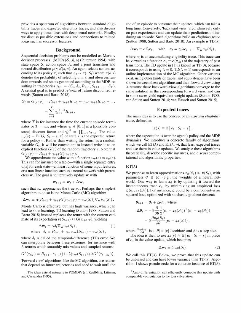
Figure 2: In the same setting as Figure 1, we show later valueestimates after more rewards have been observed. TD(0)learns slowly but steadily, TD(λ) learns faster but with highervariance, and ET(λ) learns both fast and stable.

Interpretation This result implies that linear ET(λ, η) con-verges under similar conditions as linear TD(λ′) for λ′ = λ·η.In particular, when Θ is non-singular, using the approxima-tion zΘ(s) = Θx(s) in ET(λ, 0) = ET(λ) implies conver-gence to the fixed point of TD(0).

Though ET(λ, η) and TD(λη) have the same fixed point,the algorithms are not equivalent. In general, their updatesare not the same. Linear approximations are more generalthan tabular functions (which are linear functions of a indi-cator vector for the current state), and we have already seenin Figure 1 that ET(λ) behaves quite differently from bothTD(0) and TD(λ), and we have seen its variance can be lowerin Propositions 1 and 2. Interestingly, Θ resembles a precon-ditioner that speeds up the linear semi-gradient TD update,similar to how second-order optimisation algorithms (Amari1998; Martens 2016) precondition the gradient updates.

Empirical analysisFrom the insights above, we expect that ET(λ) yields lowerprediction errors because it has lower variance and aggre-gates information across episodes better. In this section weempirically investigate expected traces in several experiments.Whenever we refer to ET(λ), this is equivalent to ET(λ, 0).

An open worldFirst consider the grid world depicted in Figure 1. The agentrandomly moves right or down (excluding moves that wouldhit a wall), starting from the top-left corner. Any action in thebottom-right corner terminates the episode with +1 rewardwith probability 0.2, and 0 otherwise. All other rewards are 0.

Figure 1 shows the value estimates after the first posi-tive reward, which occurred in the seventh episode. TD(0)updated a single state, TD(λ) updated earlier states in thatepisode, and ET(λ) additionally updated states from previousepisodes. Figure 2 shows the values after the second reward,and after roughly 20, 200, and 2000 rewards (or 100, 1000,and 10, 000 episodes, respectively). ET(λ) converged fasterthan TD(0), which propagated information slowly, and than

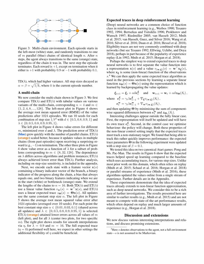
Figure 3: Multi-chain environment. Each episode starts inthe left-most (white) state, and randomly transitions to oneof m parallel (blue) chains of identical length n. After nsteps, the agent always transitions to the same (orange) state,regardless of the chain it was in. The next step the episodeterminates. Each reward is +1, except on termination when iteither is +1 with probability 0.9 or −1 with probability 0.1.

TD(λ), which had higher variance. All step sizes decayed asα = β =

√1/k, where k is the current episode number.

A multi-chainWe now consider the multi-chain shown in Figure 3. We firstcompare TD(λ) and ET(λ) with tabular values on variousvariants of the multi-chain, corresponding n = 4 and m ∈{1, 2, 4, 8, ..., 128}. The left-most plot in Figure 4 showsthe average root mean squared error (RMSE) of the valuepredictions after 1024 episodes. We ran 10 seeds for eachcombination of step size 1/td with d ∈ {0.5, 0.8, 0.9, 1} andλ ∈ {0, 0.5, 0.8, 0.9, 0.95, 1}.

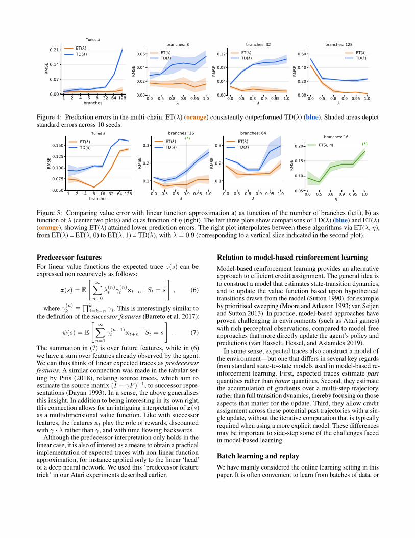
The left plot in Figure 4 shows value errors for differentm, minimized over d and λ. The prediction error of TD(λ)(blue) grew quickly with the number of parallel chains. ET(λ)(orange) scaled better, because it updates values in multiplechains (from past episodes) upon receiving a surprising re-ward (e.g.,−1) on termination. The other three plots in Figure4 show value error as a function of λ for a subset of prob-lems corresponding to m ∈ {8, 32, 128}. The dependenceon λ differs across algorithms and problem instances; ET(λ)always achieved lower error than TD(λ). Further analysis,including on step-size sensitivity, is included in the appendix.

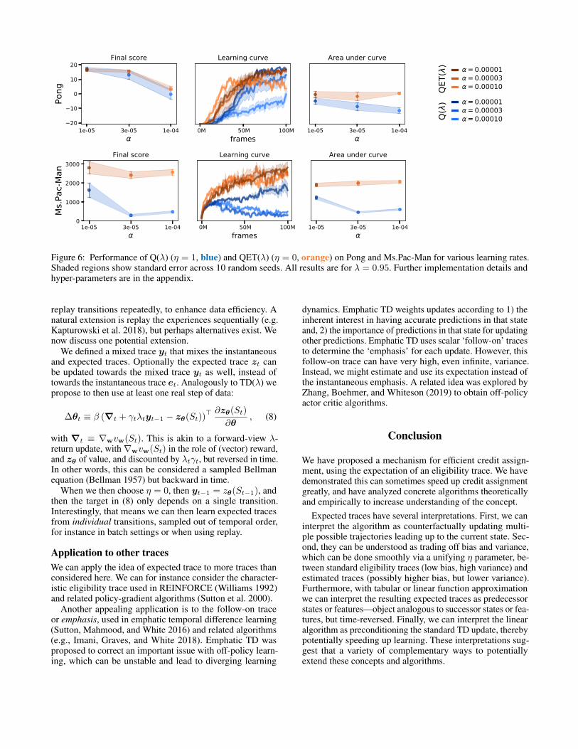
Next, we encode each state with a feature vector x(s)containing a binary indicator vector of the branch, a binaryindicator of the progress along the chain, a bias that alwaysequals one, and two binary features indicating when we arein the start (white) or bottleneck (orange) state. We extendthe lengths of the chains to n = 16. Both TD(λ) and ET(λ)use a linear value function vw(s) = w>x(s), and ET(λ)uses a linear expected trace zΘ(s) = Θx(s). All updatesuse the same constant step size α. The left plot in Figure5 shows the average root mean squared value error after1024 episodes (averaged over 10 seeds). For each point thebest constant step size α ∈ {0.01, 0.03, 0.1} (shared acrossall updates) and λ ∈ {0, 0.5, 0.8, 0.9, 0.95, 1} is selected.ET(λ) (orange) attained lower errors across all values of m(left plot), and for all λ (center two plots, for two specificm). The right plot shows results for smooth interpolationsvia η, for λ = 0.9 and m = 16. The full expected trace(η = 0) performed well here, we expect in other settings theadditional flexibility of η could be beneficial.

Expected traces in deep reinforcement learning(Deep) neural networks are a common choice of functionclass in reinforcement learning (e.g., Werbos 1990; Tesauro1992, 1994; Bertsekas and Tsitsiklis 1996; Prokhorov andWunsch 1997; Riedmiller 2005; van Hasselt 2012; Mnihet al. 2015; van Hasselt, Guez, and Silver 2016; Wang et al.2016; Silver et al. 2016; Duan et al. 2016; Hessel et al. 2018).Eligibility traces are not very commonly combined with deepnetworks (but see Tesauro 1992; Elfwing, Uchibe, and Doya2018), perhaps in part because of the popularity of experiencereplay (Lin 1992; Mnih et al. 2015; Horgan et al. 2018).

Perhaps the simplest way to extend expected traces to deepneural networks is to first separate the value function intoa representation x(s) and a value v(w,ξ)(s) = w>xξ(s),where xξ is some (non-linear) function of the observationss.4 We can then apply the same expected trace algorithm asused in the previous sections by learning a separate linearfunction zΘ(s) = Θx(s) using the representation which islearned by backpropagating the value updates:

ξt+1 = ξt + αδeξt and wt+1 = wt + αδzΘ(St) ,

where eξt = γtλeξt−1 +∇ξv(w,ξ)(St) ,

ewt = γtλe

wt−1 +∇wv(w,ξ)(St) ,

and then updating Θ by minimising the sum of component-wise squared differences between ew

t and zΘt(St).

Interesting challenges appear outside the fully linear case.First, the representation will itself be updated and will haveits own trace eξt . Second, in the control case we optimisebehaviour: the policy will change. Both these properties ofthe non-linear control setting imply that the expected tracesmust track a non-stationary target. We found that being able totrack this rather quickly improves performance: the expectedtrace parameters Θ in the following experiment were updatedwith a step size of β = 0.1.

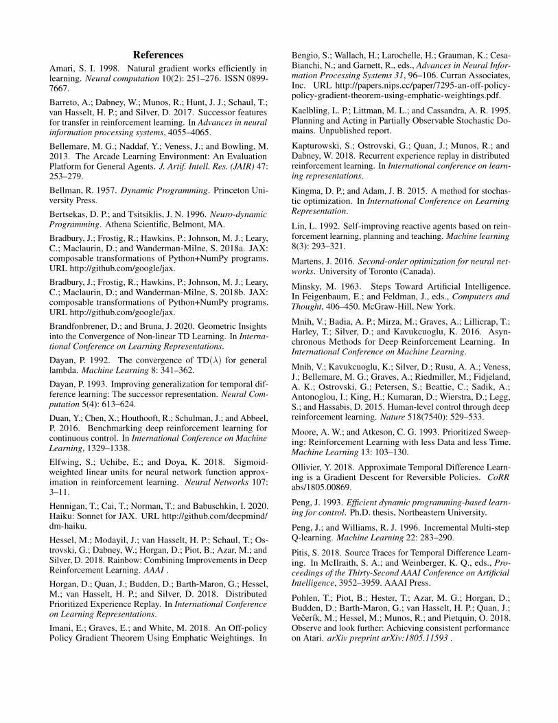
We tested this idea on two canonical Atari games: Pong andMs. Pac-Man. The results in Figure 6 show that the expectedtraces helped speed up learning compared to the baselinewhich uses accumulating traces, for various step sizes. Unlikemost prior work on this domain, which often relies on replay(Mnih et al. 2015; Schaul et al. 2016; Horgan et al. 2018)or parallel streams of experience (Mnih et al. 2016), thesealgorithms updated the values online from a single stream ofexperience. Further details are in the Appendix.

These experiments demonstrate that the idea of expectedtraces already extends to non-linear function approximation,such as deep neural networks. We consider this to be a richarea of further investigations. The results presented here aresimilar to earlier results (e.g., Mnih et al. 2015) and are notmeant to compete with state-of-the-art performance results,which often depend on replay and much larger amounts ofexperience (e.g., Horgan et al. 2018).

Discussion and extensionsWe now discuss various interesting interpretations and rela-tions, and discuss promising extensions.

4Here s denotes observations to the agent, not a full environmentstate—s is not assumed to be Markovian.

1 2 4 6 8 32 64 128branches

0.00

0.07

0.14

0.21RM

SETuned

ET( )TD( )

0.0 0.5 0.8 0.9 0.95 1.00.00

0.02

0.04

0.06

RMSE

branches: 8ET( )TD( )

0.0 0.5 0.8 0.9 0.95 1.00.00

0.04

0.08

0.12

RMSE

branches: 32ET( )TD( )

0.0 0.5 0.8 0.9 0.95 1.00.00

0.20

0.40

0.60

RMSE

branches: 128ET( )TD( )

Figure 4: Prediction errors in the multi-chain. ET(λ) (orange) consistently outperformed TD(λ) (blue). Shaded areas depictstandard errors across 10 seeds.

1 2 4 8 16 32 64 128branches

0.050

0.075

0.100

0.125

0.150

RMSE

Tuned

ET( )TD( )

0.0 0.5 0.8 0.9 0.95 1.0

0.1

0.2

0.3RM

SE(*)

branches: 16ET( ) TD( )

0.0 0.5 0.8 0.9 0.95 1.0

0.1

0.2

0.3

RMSE

branches: 64ET( ) TD( )

0.0 0.5 0.8 0.9 0.95 1.00.05

0.10

0.15

0.20

RMSE

(*)branches: 16

ET( , )

Figure 5: Comparing value error with linear function approximation a) as function of the number of branches (left), b) asfunction of λ (center two plots) and c) as function of η (right). The left three plots show comparisons of TD(λ) (blue) and ET(λ)(orange), showing ET(λ) attained lower prediction errors. The right plot interpolates between these algorithms via ET(λ, η),from ET(λ) = ET(λ, 0) to ET(λ, 1) = TD(λ), with λ = 0.9 (corresponding to a vertical slice indicated in the second plot).

Predecessor featuresFor linear value functions the expected trace z(s) can beexpressed non recursively as follows:

z(s) = E

[ ∞∑n=0

λ(n)t γ

(n)t xt−n | St = s

], (6)

where γ(n)k ≡∏kj=k−n γj . This is interestingly similar to

the definition of the successor features (Barreto et al. 2017):

ψ(s) = E

[ ∞∑n=1

γ(n−1)t xt+n | St = s

]. (7)

The summation in (7) is over future features, while in (6)we have a sum over features already observed by the agent.We can thus think of linear expected traces as predecessorfeatures. A similar connection was made in the tabular set-ting by Pitis (2018), relating source traces, which aim toestimate the source matrix (I − γP )−1, to successor repre-sentations (Dayan 1993). In a sense, the above generalisesthis insight. In addition to being interesting in its own right,this connection allows for an intriguing interpretation of z(s)as a multidimensional value function. Like with successorfeatures, the features xt play the role of rewards, discountedwith γ · λ rather than γ, and with time flowing backwards.

Although the predecessor interpretation only holds in thelinear case, it is also of interest as a means to obtain a practicalimplementation of expected traces with non-linear functionapproximation, for instance applied only to the linear ‘head’of a deep neural network. We used this ‘predecessor featuretrick’ in our Atari experiments described earlier.

Relation to model-based reinforcement learningModel-based reinforcement learning provides an alternativeapproach to efficient credit assignment. The general idea isto construct a model that estimates state-transition dynamics,and to update the value function based upon hypotheticaltransitions drawn from the model (Sutton 1990), for exampleby prioritised sweeping (Moore and Atkeson 1993; van Seijenand Sutton 2013). In practice, model-based approaches haveproven challenging in environments (such as Atari games)with rich perceptual observations, compared to model-freeapproaches that more directly update the agent’s policy andpredictions (van Hasselt, Hessel, and Aslanides 2019).

In some sense, expected traces also construct a model ofthe environment—but one that differs in several key regardsfrom standard state-to-state models used in model-based re-inforcement learning. First, expected traces estimate pastquantities rather than future quantities. Second, they estimatethe accumulation of gradients over a multi-step trajectory,rather than full transition dynamics, thereby focusing on thoseaspects that matter for the update. Third, they allow creditassignment across these potential past trajectories with a sin-gle update, without the iterative computation that is typicallyrequired when using a more explicit model. These differencesmay be important to side-step some of the challenges facedin model-based learning.

Batch learning and replayWe have mainly considered the online learning setting in thispaper. It is often convenient to learn from batches of data, or

0M 50M 100Mframes

Learning curve

1e-05 3e-05 1e-0420

10

0

10

20Po

ngFinal score

1e-05 3e-05 1e-04

Area under curve

QET(

) = 0.00001= 0.00003= 0.00010

Q() = 0.00001

= 0.00003= 0.00010

0M 50M 100Mframes

Learning curve

1e-05 3e-05 1e-040

1000

2000

3000

Ms.P

ac-M

an

Final score

1e-05 3e-05 1e-04

Area under curve

Figure 6: Performance of Q(λ) (η = 1, blue) and QET(λ) (η = 0, orange) on Pong and Ms.Pac-Man for various learning rates.Shaded regions show standard error across 10 random seeds. All results are for λ = 0.95. Further implementation details andhyper-parameters are in the appendix.

replay transitions repeatedly, to enhance data efficiency. Anatural extension is replay the experiences sequentially (e.g.Kapturowski et al. 2018), but perhaps alternatives exist. Wenow discuss one potential extension.

We defined a mixed trace yt that mixes the instantaneousand expected traces. Optionally the expected trace zt canbe updated towards the mixed trace yt as well, instead oftowards the instantaneous trace et. Analogously to TD(λ) wepropose to then use at least one real step of data:

∆θt ≡ β (∇t + γtλtyt−1 − zθ(St))> ∂zθ(St)

∂θ, (8)

with ∇t ≡ ∇wvw(St). This is akin to a forward-view λ-return update, with∇wvw(St) in the role of (vector) reward,and zθ of value, and discounted by λtγt, but reversed in time.In other words, this can be considered a sampled Bellmanequation (Bellman 1957) but backward in time.

When we then choose η = 0, then yt−1 = zθ(St−1), andthen the target in (8) only depends on a single transition.Interestingly, that means we can then learn expected tracesfrom individual transitions, sampled out of temporal order,for instance in batch settings or when using replay.

Application to other tracesWe can apply the idea of expected trace to more traces thanconsidered here. We can for instance consider the character-istic eligibility trace used in REINFORCE (Williams 1992)and related policy-gradient algorithms (Sutton et al. 2000).

Another appealing application is to the follow-on traceor emphasis, used in emphatic temporal difference learning(Sutton, Mahmood, and White 2016) and related algorithms(e.g., Imani, Graves, and White 2018). Emphatic TD wasproposed to correct an important issue with off-policy learn-ing, which can be unstable and lead to diverging learning

dynamics. Emphatic TD weights updates according to 1) theinherent interest in having accurate predictions in that stateand, 2) the importance of predictions in that state for updatingother predictions. Emphatic TD uses scalar ‘follow-on’ tracesto determine the ‘emphasis’ for each update. However, thisfollow-on trace can have very high, even infinite, variance.Instead, we might estimate and use its expectation instead ofthe instantaneous emphasis. A related idea was explored byZhang, Boehmer, and Whiteson (2019) to obtain off-policyactor critic algorithms.

Conclusion

We have proposed a mechanism for efficient credit assign-ment, using the expectation of an eligibility trace. We havedemonstrated this can sometimes speed up credit assignmentgreatly, and have analyzed concrete algorithms theoreticallyand empirically to increase understanding of the concept.

Expected traces have several interpretations. First, we caninterpret the algorithm as counterfactually updating multi-ple possible trajectories leading up to the current state. Sec-ond, they can be understood as trading off bias and variance,which can be done smoothly via a unifying η parameter, be-tween standard eligibility traces (low bias, high variance) andestimated traces (possibly higher bias, but lower variance).Furthermore, with tabular or linear function approximationwe can interpret the resulting expected traces as predecessorstates or features—object analogous to successor states or fea-tures, but time-reversed. Finally, we can interpret the linearalgorithm as preconditioning the standard TD update, therebypotentially speeding up learning. These interpretations sug-gest that a variety of complementary ways to potentiallyextend these concepts and algorithms.

ReferencesAmari, S. I. 1998. Natural gradient works efficiently inlearning. Neural computation 10(2): 251–276. ISSN 0899-7667.

Barreto, A.; Dabney, W.; Munos, R.; Hunt, J. J.; Schaul, T.;van Hasselt, H. P.; and Silver, D. 2017. Successor featuresfor transfer in reinforcement learning. In Advances in neuralinformation processing systems, 4055–4065.

Bellemare, M. G.; Naddaf, Y.; Veness, J.; and Bowling, M.2013. The Arcade Learning Environment: An EvaluationPlatform for General Agents. J. Artif. Intell. Res. (JAIR) 47:253–279.

Bellman, R. 1957. Dynamic Programming. Princeton Uni-versity Press.

Bertsekas, D. P.; and Tsitsiklis, J. N. 1996. Neuro-dynamicProgramming. Athena Scientific, Belmont, MA.

Bradbury, J.; Frostig, R.; Hawkins, P.; Johnson, M. J.; Leary,C.; Maclaurin, D.; and Wanderman-Milne, S. 2018a. JAX:composable transformations of Python+NumPy programs.URL http://github.com/google/jax.

Bradbury, J.; Frostig, R.; Hawkins, P.; Johnson, M. J.; Leary,C.; Maclaurin, D.; and Wanderman-Milne, S. 2018b. JAX:composable transformations of Python+NumPy programs.URL http://github.com/google/jax.

Brandfonbrener, D.; and Bruna, J. 2020. Geometric Insightsinto the Convergence of Non-linear TD Learning. In Interna-tional Conference on Learning Representations.

Dayan, P. 1992. The convergence of TD(λ) for generallambda. Machine Learning 8: 341–362.

Dayan, P. 1993. Improving generalization for temporal dif-ference learning: The successor representation. Neural Com-putation 5(4): 613–624.

Duan, Y.; Chen, X.; Houthooft, R.; Schulman, J.; and Abbeel,P. 2016. Benchmarking deep reinforcement learning forcontinuous control. In International Conference on MachineLearning, 1329–1338.

Elfwing, S.; Uchibe, E.; and Doya, K. 2018. Sigmoid-weighted linear units for neural network function approx-imation in reinforcement learning. Neural Networks 107:3–11.

Hennigan, T.; Cai, T.; Norman, T.; and Babuschkin, I. 2020.Haiku: Sonnet for JAX. URL http://github.com/deepmind/dm-haiku.

Hessel, M.; Modayil, J.; van Hasselt, H. P.; Schaul, T.; Os-trovski, G.; Dabney, W.; Horgan, D.; Piot, B.; Azar, M.; andSilver, D. 2018. Rainbow: Combining Improvements in DeepReinforcement Learning. AAAI .

Horgan, D.; Quan, J.; Budden, D.; Barth-Maron, G.; Hessel,M.; van Hasselt, H. P.; and Silver, D. 2018. DistributedPrioritized Experience Replay. In International Conferenceon Learning Representations.

Imani, E.; Graves, E.; and White, M. 2018. An Off-policyPolicy Gradient Theorem Using Emphatic Weightings. In

Bengio, S.; Wallach, H.; Larochelle, H.; Grauman, K.; Cesa-Bianchi, N.; and Garnett, R., eds., Advances in Neural Infor-mation Processing Systems 31, 96–106. Curran Associates,Inc. URL http://papers.nips.cc/paper/7295-an-off-policy-policy-gradient-theorem-using-emphatic-weightings.pdf.

Kaelbling, L. P.; Littman, M. L.; and Cassandra, A. R. 1995.Planning and Acting in Partially Observable Stochastic Do-mains. Unpublished report.

Kapturowski, S.; Ostrovski, G.; Quan, J.; Munos, R.; andDabney, W. 2018. Recurrent experience replay in distributedreinforcement learning. In International conference on learn-ing representations.

Kingma, D. P.; and Adam, J. B. 2015. A method for stochas-tic optimization. In International Conference on LearningRepresentation.

Lin, L. 1992. Self-improving reactive agents based on rein-forcement learning, planning and teaching. Machine learning8(3): 293–321.

Martens, J. 2016. Second-order optimization for neural net-works. University of Toronto (Canada).

Minsky, M. 1963. Steps Toward Artificial Intelligence.In Feigenbaum, E.; and Feldman, J., eds., Computers andThought, 406–450. McGraw-Hill, New York.

Mnih, V.; Badia, A. P.; Mirza, M.; Graves, A.; Lillicrap, T.;Harley, T.; Silver, D.; and Kavukcuoglu, K. 2016. Asyn-chronous Methods for Deep Reinforcement Learning. InInternational Conference on Machine Learning.

Mnih, V.; Kavukcuoglu, K.; Silver, D.; Rusu, A. A.; Veness,J.; Bellemare, M. G.; Graves, A.; Riedmiller, M.; Fidjeland,A. K.; Ostrovski, G.; Petersen, S.; Beattie, C.; Sadik, A.;Antonoglou, I.; King, H.; Kumaran, D.; Wierstra, D.; Legg,S.; and Hassabis, D. 2015. Human-level control through deepreinforcement learning. Nature 518(7540): 529–533.

Moore, A. W.; and Atkeson, C. G. 1993. Prioritized Sweep-ing: Reinforcement Learning with less Data and less Time.Machine Learning 13: 103–130.

Ollivier, Y. 2018. Approximate Temporal Difference Learn-ing is a Gradient Descent for Reversible Policies. CoRRabs/1805.00869.

Peng, J. 1993. Efficient dynamic programming-based learn-ing for control. Ph.D. thesis, Northeastern University.

Peng, J.; and Williams, R. J. 1996. Incremental Multi-stepQ-learning. Machine Learning 22: 283–290.

Pitis, S. 2018. Source Traces for Temporal Difference Learn-ing. In McIlraith, S. A.; and Weinberger, K. Q., eds., Pro-ceedings of the Thirty-Second AAAI Conference on ArtificialIntelligence, 3952–3959. AAAI Press.

Pohlen, T.; Piot, B.; Hester, T.; Azar, M. G.; Horgan, D.;Budden, D.; Barth-Maron, G.; van Hasselt, H. P.; Quan, J.;Vecerık, M.; Hessel, M.; Munos, R.; and Pietquin, O. 2018.Observe and look further: Achieving consistent performanceon Atari. arXiv preprint arXiv:1805.11593 .

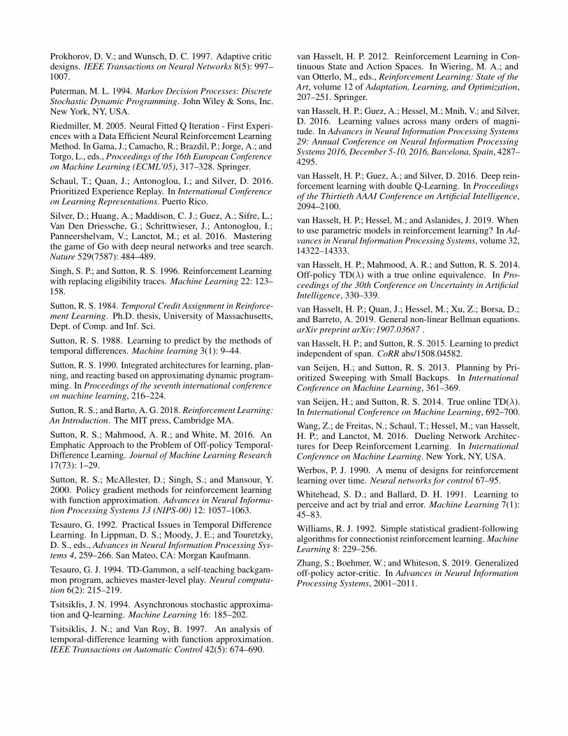
Prokhorov, D. V.; and Wunsch, D. C. 1997. Adaptive criticdesigns. IEEE Transactions on Neural Networks 8(5): 997–1007.

Puterman, M. L. 1994. Markov Decision Processes: DiscreteStochastic Dynamic Programming. John Wiley & Sons, Inc.New York, NY, USA.

Riedmiller, M. 2005. Neural Fitted Q Iteration - First Experi-ences with a Data Efficient Neural Reinforcement LearningMethod. In Gama, J.; Camacho, R.; Brazdil, P.; Jorge, A.; andTorgo, L., eds., Proceedings of the 16th European Conferenceon Machine Learning (ECML’05), 317–328. Springer.

Schaul, T.; Quan, J.; Antonoglou, I.; and Silver, D. 2016.Prioritized Experience Replay. In International Conferenceon Learning Representations. Puerto Rico.

Silver, D.; Huang, A.; Maddison, C. J.; Guez, A.; Sifre, L.;Van Den Driessche, G.; Schrittwieser, J.; Antonoglou, I.;Panneershelvam, V.; Lanctot, M.; et al. 2016. Masteringthe game of Go with deep neural networks and tree search.Nature 529(7587): 484–489.

Singh, S. P.; and Sutton, R. S. 1996. Reinforcement Learningwith replacing eligibility traces. Machine Learning 22: 123–158.

Sutton, R. S. 1984. Temporal Credit Assignment in Reinforce-ment Learning. Ph.D. thesis, University of Massachusetts,Dept. of Comp. and Inf. Sci.

Sutton, R. S. 1988. Learning to predict by the methods oftemporal differences. Machine learning 3(1): 9–44.

Sutton, R. S. 1990. Integrated architectures for learning, plan-ning, and reacting based on approximating dynamic program-ming. In Proceedings of the seventh international conferenceon machine learning, 216–224.

Sutton, R. S.; and Barto, A. G. 2018. Reinforcement Learning:An Introduction. The MIT press, Cambridge MA.

Sutton, R. S.; Mahmood, A. R.; and White, M. 2016. AnEmphatic Approach to the Problem of Off-policy Temporal-Difference Learning. Journal of Machine Learning Research17(73): 1–29.

Sutton, R. S.; McAllester, D.; Singh, S.; and Mansour, Y.2000. Policy gradient methods for reinforcement learningwith function approximation. Advances in Neural Informa-tion Processing Systems 13 (NIPS-00) 12: 1057–1063.

Tesauro, G. 1992. Practical Issues in Temporal DifferenceLearning. In Lippman, D. S.; Moody, J. E.; and Touretzky,D. S., eds., Advances in Neural Information Processing Sys-tems 4, 259–266. San Mateo, CA: Morgan Kaufmann.

Tesauro, G. J. 1994. TD-Gammon, a self-teaching backgam-mon program, achieves master-level play. Neural computa-tion 6(2): 215–219.

Tsitsiklis, J. N. 1994. Asynchronous stochastic approxima-tion and Q-learning. Machine Learning 16: 185–202.

Tsitsiklis, J. N.; and Van Roy, B. 1997. An analysis oftemporal-difference learning with function approximation.IEEE Transactions on Automatic Control 42(5): 674–690.

van Hasselt, H. P. 2012. Reinforcement Learning in Con-tinuous State and Action Spaces. In Wiering, M. A.; andvan Otterlo, M., eds., Reinforcement Learning: State of theArt, volume 12 of Adaptation, Learning, and Optimization,207–251. Springer.van Hasselt, H. P.; Guez, A.; Hessel, M.; Mnih, V.; and Silver,D. 2016. Learning values across many orders of magni-tude. In Advances in Neural Information Processing Systems29: Annual Conference on Neural Information ProcessingSystems 2016, December 5-10, 2016, Barcelona, Spain, 4287–4295.van Hasselt, H. P.; Guez, A.; and Silver, D. 2016. Deep rein-forcement learning with double Q-Learning. In Proceedingsof the Thirtieth AAAI Conference on Artificial Intelligence,2094–2100.van Hasselt, H. P.; Hessel, M.; and Aslanides, J. 2019. Whento use parametric models in reinforcement learning? In Ad-vances in Neural Information Processing Systems, volume 32,14322–14333.van Hasselt, H. P.; Mahmood, A. R.; and Sutton, R. S. 2014.Off-policy TD(λ) with a true online equivalence. In Pro-ceedings of the 30th Conference on Uncertainty in ArtificialIntelligence, 330–339.van Hasselt, H. P.; Quan, J.; Hessel, M.; Xu, Z.; Borsa, D.;and Barreto, A. 2019. General non-linear Bellman equations.arXiv preprint arXiv:1907.03687 .van Hasselt, H. P.; and Sutton, R. S. 2015. Learning to predictindependent of span. CoRR abs/1508.04582.van Seijen, H.; and Sutton, R. S. 2013. Planning by Pri-oritized Sweeping with Small Backups. In InternationalConference on Machine Learning, 361–369.van Seijen, H.; and Sutton, R. S. 2014. True online TD(λ).In International Conference on Machine Learning, 692–700.Wang, Z.; de Freitas, N.; Schaul, T.; Hessel, M.; van Hasselt,H. P.; and Lanctot, M. 2016. Dueling Network Architec-tures for Deep Reinforcement Learning. In InternationalConference on Machine Learning. New York, NY, USA.Werbos, P. J. 1990. A menu of designs for reinforcementlearning over time. Neural networks for control 67–95.Whitehead, S. D.; and Ballard, D. H. 1991. Learning toperceive and act by trial and error. Machine Learning 7(1):45–83.Williams, R. J. 1992. Simple statistical gradient-followingalgorithms for connectionist reinforcement learning. MachineLearning 8: 229–256.Zhang, S.; Boehmer, W.; and Whiteson, S. 2019. Generalizedoff-policy actor-critic. In Advances in Neural InformationProcessing Systems, 2001–2011.

AppendixProof of Lemma 1We start with a formal definition of a Markov state:Definition 1. Markov property: we say a state s is Markov if

p(Rt+1, St+1|At, St, Rt−1, At−1, St−1...) = p(Rt+1, St+1|At, St).Next, we show that a Markov state implies a similar property for the transition probabilities induced by a policy π:Property 1. Let pπ be the transition probabilities induced by policy π. Then, if s is Markov, we have that

pπ(Rt+1, St+1|St, Rt−1, At−1, St−1...) = pπ(Rt+1, St+1|St).Proof.

pπ(Rt+1, St+1|St, Rt−1, At−1, St−1...) =

∫a

π(a|St)p(St+1, Rt+1|At = a, St, Rt−1, At−1, St−1...)da (9)

=

∫a

π(a|St)p(St+1, Rt+1|At = a, St)da. (Markov property)

Using the above, we can prove Lemma 1:Lemma 1. If s is Markov, then E [ δtet | St = s ] = E [ δt | St = s ]E [ et | St = s ].

Proof. First note that the expectations above are with respect to the transition probabilities pπ as defined in (9). That noted, theresult trivially follows from the fact that, when s is Markov, the two random variables δt and et are independent conditioned onSt. To see why this is so, note that δt is defined as

δt = Rt+1 + γt+1vw(St+1)− vw(St). (10)

Since we are conditioning on the event that St = s, the only two random quantities in the definition of δt are Rt+1 and St+1.Thus, because s is Markov, we have that

pπ(δt|St, Rt, St−1, Rt−1, ...) = pπ(δt|St), (Property 1)

that is, St fully defines the distribution of δt. This means that pπ(δt|St, Xt′) = pπ(δt|St) for any t′ ≤ t, where Xt′ is a randomvariable that only depends on events that occurred up to time t′. Replacing Xt′ with et, we have that pπ(δt|St, et) = pπ(δt|St),which implies that δt and et are independent conditioned on St.

Proof of Proposition 2Proposition 2. Let et an instantaneous trace vector. Then let zt(s) be the empirical mean zt(s) = 1

nt(s)

∑nt(s)i etsi , where tsi -s

denote past times when we have been in state s, that is Stsi = s, and nt(s) is the number of visits to s in the first t steps. Considerthe expected trace algorithm wt+1 = wt +αtδtzt. If St is Markov, the expectation of this update is equal to the expected updatewith instantaneous traces et, while attaining a potentially lower variance:

E [αtδtzt(St) | St ] = E [αtδtet | St ] andV[αtδtzt(St) | St] ≤ V[αtδtet | St] ,

where the second inequality holds component-wise. The inequality is strict when V[et | St] > 0.

Proof. We have

E [αtδtet | St = s ] = E [αtδt | St = s ]E [ et | St = s ] (as s is Markov)

= E [αtδt | St = s ]E [ zt | St = s ] (as zt = 1n

∑ni etsi )

= E [αtδtzt | St = s ] .

Now let us look at the conditional variance for each of the dimension of the update vector αtδtzt: V[αtδtzt,i | St = s], wherezt,i denotes the i-th component of vector zt.

V[αtδtzt,i | St = s]

= E[

(αtδtzt,i)2 | St = s

]− E [αtδtzt,i | St = s ]

2

= E[α2t δ

2t (zt,i)

2 | St = s]− E [αtδt | St = s ]

2 E [ zt,i | St = s ]2

= E[α2t δ

2t | St = s

]E[

(zt,i)2 | St = s

]− E [αtδt | St = s ]

2 E [ zt,i | St = s ]2

By a similar argument, we have

V[αtδtet,i | St = s]

= E[α2t δ

2t | St = s

]E[

(et,i)2 | St = s

]− E [αtδt | St = s ]

2 E [ et,i | St = s ]2

Now, we also know that E [ zt | St = s ] = E [ et | St = s ] = µt, as zt is the empirical mean of et. Thus we also have,component-wise,

E [ zt,i | St = s ] = E [ et,i | St = s ] = µt,i

Moreover, from the same reason we have that V(zt,i|St = s) = 1nsV(et,i|St = s). Thus we obtain:

V[αtδtzt,i | St = s] = E[α2t δ

2t | St = s

]E[zt,i(zt,i)

T | St = s]− E [αtδt | St = s ]

2µ2t,i

Thus:

V[αtδtzt,i | St = s]− V[αtδtet,i | St = s]

= E[α2t δ

2t | St = s

] (E[zt,i(zt,i)

T | St = s]− E

[et,i(et,i)

T | St = s])︸ ︷︷ ︸

≤0, from definition of zt,i

≤ 0 ,

with equality holding, if and only if:

i E[

(zt,i)2 | St = s

]= E

[(et,i)

2 | St = s]⇒ V(zt,i|St = s) = V(et,i|St = s), but V(zt,i|St = s) = 1

nsV(et,i|St = s)

by definition of zt,i as the running mean on samples et,i. This can only happen for ns = 1, or in the absence of stochasticity,for every state s. Thus, in the most general case, this implies V(zt,i|St = s) = V(et,i|St = s) = 0; or

ii E[α2t δ

2t | St = s

]= 0⇒ δt = 0

Thus, we have equality only with we have exactly one sample for the average zt so far, or only one sample is needed (thus ztand et are not actual random variables and there is only one deterministic path to s); or when the TD errors are zero for alltransitions following s.

Properties of mixture tracesIn this section we explore and proof some of the properties of the proposed mixture trace, defined in Equation (3) in the maintext and repeated here:

yt = (1− η)zθ(St) + η(γtλtyt−1 +∇wvw(St)

). (3)

The proofs, in this section we will use the notation xt to denote the features used in a linear approximation for the valuefunction(s) constructed. Just note that this term can be substituted, in general, by the gradient term ∇wvw(St) in the equationabove.Proposition 3. The mixture trace yt defined in (3) can be written as yt = µyt−1 + ut with decay parameter µ = ηγλ andsignal ut = (1− η)zθ(St) + η ∇wvw(St), such that

yt =

t∑k=0

(ηγλ)k [(1− η)zθ(St−k) + η ∇wvw(St−k)] . (5)

Proof. As mentioned before, under a linear parameterization∇wvw(St) = x(St) := xt Let us start with the definition of themixture trace yt:

yt = (1− η)zt + η(γtλtyt−1 + xt)

= [(1− η)zt + ηxt] + ηγtλtyt−1

= [(1− η)zt + ηxt] + ηγtλt [(1− η)zt−1 + ηxt−1] + η2γtλtγt−1λt−1yt−2

= (1− η)[zt + ηγtλtzt−1 + η2γtλtγt−1λt−1zt−2 + · · ·

]+

+ η[xt + ηγtλtxt−1 + η2γtλtγt−1λt−1xt−2 + · · ·

]= (1− η)

t∑k=0

(ηγλ)kzt−k + η

t∑k=0

(ηγλ)kxt−k

=

t∑k=0

(ηγλ)k [(1− η)zt−k + ηxt−k]

Substituting xt in the above derivation by ∇wvw(St) leads to (3).

Proposition 4. When using approximations zΘ(s) = Θx(s) and vw(s) = w>x(s) then, if (1 − η)Θ + ηI is non-singular,ET(λ, η) has the same fixed point as TD(λη).

Proof. By Proposition 3 we have that yt can be re-written as:

yt =

t∑k=0

(ηγλ)k [(1− η)zθ(St−k) + ηx(St−k)]

=

t∑k=0

(ηγλ)k [(1− η)Θx(St−k) + ηx(St−k)] (11)

= [(1− η)Θ + ηI]t∑

k=0

(ηγλ)kx(St−k)︸ ︷︷ ︸instantaneous trace eληt

. (12)

We examine the fixed point w∗ of the algorithm using this approximation of the expected trace:

E [ δtyt ] = E[yt(Rt+1 + γx(St+1)>w∗ − x(St)

>w∗)]

= 0 .

This implies the fixed point is

w∗ = E[yt(γx(St+1)− x(St))

> ]−1 E [ytRt+1 ] .

Now, plugging in the relation in (12) above, we get:

w∗ = E[

[(1− η)Θ + ηI] eληt (γx(St+1)− x(St))>]−1

E[

[(1− η)Θ + ηI] eληt Rt+1

]= E

[eληt (γx(St+1)− x(St))

>]−1

[(1− η)Θ + ηI]−1 [(1− η)Θ + ηI]E[eληt Rt+1

]= E

[eληt (γx(St+1)− x(St))

>]−1

E[eληt Rt+1

].

This last term is the fixed point for TD(λη).

Moreover, it is worth noting that the above equality recovers, for the extreme values of η:

• η = 1⇒ yt =∑tk=0(γλ)kxt−k (instantaneous trace for TD(λ))

• η = 0⇒ yt =∑tk=0(ηγλ)kzt−k = zt (expected trace for TD(λ))

Moreover, as the extreme values already suggest, the expected update of the mixture traces follows the TD(λ) learning, inexpectation, for all the intermediate values η ∈ (0, 1) as well, trading off variance of estimates as η approaches 0.

Proposition 5. Let eλt be a λ trace vector. Let yt = (1 − η)zt + η(γλyt−1 + xt) (as defined in (3)). Consider the ET(λ, η)algorithm wt+1 = wt + αtδtyt. For all Markov states s the expectation of this update is equal to the expected update withinstantaneous traces eλt :

E [αtδty(St)|St = s ] = E[αtδte

λt |St = s

],

for every η ∈ [0, 1] and any λ ∈ [0, 1].

Proof. Let us revisit Eq. 5 in Proposition 3:

E [yt ] = E

[t∑

k=0

(ηγλ)k [(1− η)zt−k + ηxt−k]

]

= E

[t∑

k=0

(ηγλ)k [(1− η)E [ (xt−k + γλzt−k−1) ] + ηxt−k]

]

= E

t∑k=0

(ηγλ)kxt−k + (1− η)γλt−1∑k=0

(ηγλ)k zt−k−1︸ ︷︷ ︸E[ (xt−k−1+γλzt−k−2) ]

= E

t∑k=0

(ηγλ)kxt−k + (1− η)γλt−1∑k=0

(ηγλ)kxt−k−1 + (1− η)(γλ)2t−2∑k=0

(ηγλ)k zt−k−2︸ ︷︷ ︸E[xt−k−2+γλzt−k−3 ]

= E

[t∑

k=0

(ηγλ)kxt−k + (1− η)t−1∑i=1

(γλ)it−i∑k=0

(ηγλ)kxt−k−i

]

Now, re-writing the sum, gathering all the weighting for each feature xt−k−i we get:

E [yt ] = E

[t∑

k=0

(ηγλ)kxt−k + (1− η)t−1∑i=1

(γλ)it−i∑k=0

(ηγλ)kxt−k−i

]

= E

[xt +

t∑k=1

xt−k

((ηγλ)k + (1− η)

k∑i=1

(γλ)i · (γλη)k−i)]

= E

[xt +

t∑k=1

xt−k(γλ)k

(ηk + (1− η)

k∑i=1

ηk−i)]

= E

[xt +

t∑k=1

xt−k(γλ)k

(ηk + (1− η) 1− η

k

(1− η)

)]

= E

[xt +

t∑k=1

xt−k(γλ)k

]

= E

[t∑

k=0

(γλ)kxt−k

]

Thus E [yt ] = E[∑t

k=0(γλ)kxt−k

]= E

[eλt], where eλt is the instantaneous λ trace on feature space x. Thus E [y(s) ] = zλ∗ (s) =

E[eλt]. Finally we can plug-in this result in the expected update:

E [αtδty(St)|St = s ] = E [αtδt|St = s ]E [y(St)|St = s ]

= E [αtδt|St = s ] zλ∗ (s)

= E [αtδt|St = s ]E[eλt |St = s

]= E

[αtδte

λt |St = s

].

Finally, please note that in this proposition and its proof we drop the time indices t for λ and γ parameters in the definition ofyt. This is purely to ease the notation and promote compactness in the derivation

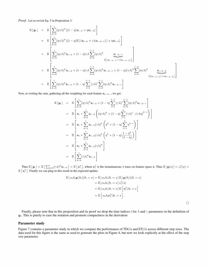
Parameter studyFigure 7 contains a parameter study in which we compare the performance of TD(λ) and ET(λ) across different step sizes. Thedata used for this figure is the same as used to generate the plots in Figure 4, but now we look explicitly at the effect of the stepsize parameter.

0.0 0.5 0.8 0.9 0.95 1.00.00

0.05

0.10

0.15

0.20

0.25

RMSE

TD( ), = 1/nTD( ), = 1/n0.9

TD( ), = 1/n0.8

TD( ), = 1/ nET( ), = 1/nET( ), = 1/n0.9

ET( ), = 1/n0.8

ET( ), = 1/ n

Figure 7: Comparison of prediction errors (lower is better) of TD(λ) and ET(λ) across different λs and different step sizes in themulti-chain world 3. The data underpinning these plots is the same as the data used for Figure 4, with 32 parallel chains. In allcases the step size was α = 1/nt(St)

d, where nt(s) =∑ti=0 I(Si = s) is the number of visits to state s in the first t time steps,

and where d is a hyper-parameter. Note that the step size is lower when the exponent is higher. We see that TD(0) performed bestwith a high step size, and that for high λ lower step sizes performed better—TD(0) with the highest step size (αt = 1/

√nt(St))

and TD(1) with the lowest step size (αt = 1/nt(St)) both performed poorly. In contrast, ET(λ) here performed well for anycombination of step size and trace parameter λ.

Experiment details for Atari experimentsFor our deep reinforcement learning experiments on Atari games, we compare to an implementation of online Q(λ). We firstdescribe this algorithm, and then describe the expected-trace variant. All the Atari experiments were run with the ALE (Bellemareet al. 2013), exactly as described in Mnih et al. (2015), including using action repeats (4x), downsampling (to 84× 84), andframe stacking. These experiments were conducted using Jax (Bradbury et al. 2018a).

In all cases, we used ε-greedy exploration (cf. Sutton and Barto 2018), with an ε that quickly decayed from 1 to 0.01 accordingto ε0 = 1 and εt = εt−1 + 0.01(0.01− εt−1). Unlike Mnih et al. (2015), we did not clip rewards, and we also did not apply anytarget normalisation (cf. van Hasselt et al. 2016) or non-linear value transformations (Pohlen et al. 2018; van Hasselt et al. 2019).We conjecture that such extensions could be beneficial for performance, but they are orthogonal to the main research questionsinvestigated here and are therefore left for future work.

Algorithm 2 Q(λ)

1: initialise w2: initialise e = 03: observe initial state S4: pick action A ∼ π(qw(S))5: v ← maxa qw(S, a)6: γ = 07: repeat8: take action A, observe R, γ′ and S′ # γ′ = 0 on a terminating transition9: v′ ← maxa qw(S′, a)

10: δ ← R+ γv′ − v11: e← γλe+∇wqw(S,A)12: ∆w← δe+ (v − qw(S,A))∇wqw(S,A)13: ∆w← transform(∆w) # e.g., ADAM-ify14: w← w + ∆w15: until done

Deep Q(λ) We assume the typical setting (e.g., Mnih et al. 2015) where we have a neural network qw that outputs |A| numbers,such that q(s, a) = qw(s)[a]. That is, we forward the observation s through network qw with weights w and |A| outputs, andthen select the ath output to represent the value of taking action a.

Algorithm 2 then works as follows. For each transition, we first compute a telescoping TD error δ = r + γ′v′ − v (line 5),where γ′ = 0 on termination (and then S′ is the first observation of the next episode) and, in our experiments, γ′ = 0.995otherwise. We update the trace e as usual (line 11), using accumulating traces. Note that the weights and, hence, trace will alsohave elements corresponding to the weights of actions that were not selected. The gradient with respect to those elements isconsidered to be zero, as is conventional.

Then, we compute a weight update ∆w = δe+ (v − qw(S,A))∇wqw(S,A). The additional term corrects for the fact thatour TD error is a telescoping error, and does not have the usual ‘− q(s, a)’ term. This is akin to the Q(λ) algorithm proposed byPeng and Williams (1996).

Finally, we transform the resulting update, using a transformation exactly like ADAM (Kingma and Adam 2015), but appliedto the update ∆w rather than a gradient. The hyper-parameters were β1 = 0.9, β2 = 0.999, and ε = 0.0001, and one of the stepsizes as given in Figure 6. We then apply the resulting transformed update by adding it to the weights (line 14).

For the Atari experiments, we used the same preprocessing and network architecture as Mnih et al. (2015), except that we used128 channels in each convolutional layer because we ran experiments on TPUs (version 3.0, using a single core per experiment)which are most efficient when using tensors where one dimension is a multiple of 128. The experiments were written using JAX(Bradbury et al. 2018b) and Haiku (Hennigan et al. 2020).

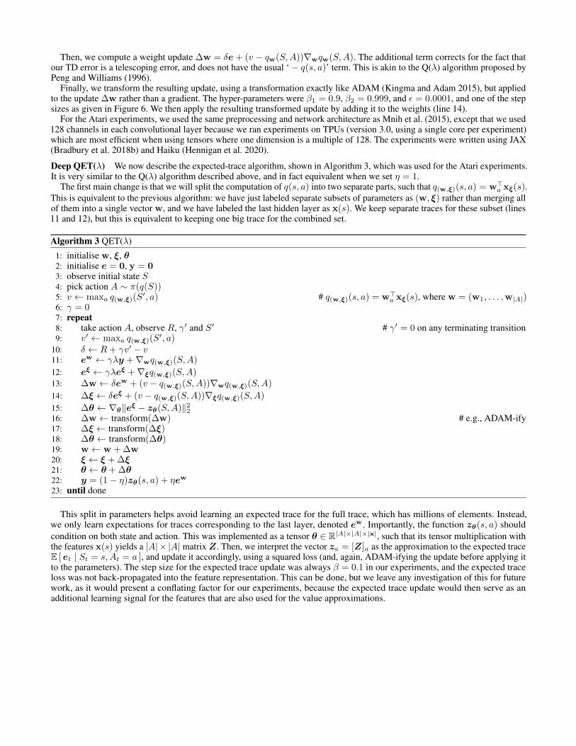
Deep QET(λ) We now describe the expected-trace algorithm, shown in Algorithm 3, which was used for the Atari experiments.It is very similar to the Q(λ) algorithm described above, and in fact equivalent when we set η = 1.

The first main change is that we will split the computation of q(s, a) into two separate parts, such that q(w,ξ)(s, a) = w>a xξ(s).This is equivalent to the previous algorithm: we have just labeled separate subsets of parameters as (w, ξ) rather than merging allof them into a single vector w, and we have labeled the last hidden layer as x(s). We keep separate traces for these subset (lines11 and 12), but this is equivalent to keeping one big trace for the combined set.

Algorithm 3 QET(λ)

1: initialise w, ξ, θ2: initialise e = 0, y = 03: observe initial state S4: pick action A ∼ π(q(S))5: v ← maxa q(w,ξ)(S

′, a) # q(w,ξ)(s, a) = w>a xξ(s), where w = (w1, . . . ,w|A|)6: γ = 07: repeat8: take action A, observe R, γ′ and S′ # γ′ = 0 on any terminating transition9: v′ ← maxa q(w,ξ)(S

′, a)10: δ ← R+ γv′ − v11: ew ← γλy +∇wq(w,ξ)(S,A)

12: eξ ← γλeξ +∇ξq(w,ξ)(S,A)13: ∆w← δew + (v − q(w,ξ)(S,A))∇wq(w,ξ)(S,A)

14: ∆ξ ← δeξ + (v − q(w,ξ)(S,A))∇ξq(w,ξ)(S,A)

15: ∆θ ← ∇θ‖eξ − zθ(S,A)‖2216: ∆w← transform(∆w) # e.g., ADAM-ify17: ∆ξ ← transform(∆ξ)18: ∆θ ← transform(∆θ)19: w← w + ∆w20: ξ ← ξ + ∆ξ21: θ ← θ + ∆θ22: y = (1− η)zθ(s, a) + ηew

23: until done

This split in parameters helps avoid learning an expected trace for the full trace, which has millions of elements. Instead,we only learn expectations for traces corresponding to the last layer, denoted ew. Importantly, the function zθ(s, a) shouldcondition on both state and action. This was implemented as a tensor θ ∈ R|A|×|A|×|x|, such that its tensor multiplication withthe features x(s) yields a |A|× |A| matrix Z. Then, we interpret the vector za = [Z]a as the approximation to the expected traceE [ et | St = s,At = a ], and update it accordingly, using a squared loss (and, again, ADAM-ifying the update before applying itto the parameters). The step size for the expected trace update was always β = 0.1 in our experiments, and the expected traceloss was not back-propagated into the feature representation. This can be done, but we leave any investigation of this for futurework, as it would present a conflating factor for our experiments, because the expected trace update would then serve as anadditional learning signal for the features that are also used for the value approximations.