Expectation propagation as a way of life∗

Andrew Gelman† Aki Vehtari‡ Pasi Jylänki§ Christian Robert¶ Nicolas Chopin‖

John P. Cunningham∗∗

15 Dec 2014

Abstract

We revisit expectation propagation (EP) as a prototype for scalable algorithms that partitionbig datasets into many parts and analyze each part in parallel to perform inference of sharedparameters. The algorithm should be particularly efficient for hierarchical models, for whichthe EP algorithm works on the shared parameters (hyperparameters) of the model.

The central idea of EP is to work at each step with a “tilted distribution” that combines thelikelihood for a part of the data with the “cavity distribution,” which is the approximate modelfor the prior and all other parts of the data. EP iteratively approximates the moments of thetilted distributions and incorporates those approximations into a global posterior approximation.As such, EP can be used to divide the computation for large models into manageable sizes. Thecomputation for each partition can be made parallel with occasional exchanging of informationbetween processes through the global posterior approximation. Moments of multivariate tilteddistributions can be approximated in various ways, including, MCMC, Laplace approximations,and importance sampling.

Keywords: Bayesian computation, big data, data partitioning, expectation propagation,hierarchical models, Stan, statistical computing

1. Background: Bayesian computation via data partitioning

Various divide-and-conquer algorithms have been proposed for fitting statistical models to largedatasets. The basic idea is to partition the data y into K pieces, y1, . . . , yK , each with likelihoodp(yk|θ), then analyze each part of the likelihood separately; and finally combine the K pieces toperform inference (typically approximately) for θ. In addition to the appeal of such algorithmsfor parallel or online computation, there is a statistical intuition that they should work well fromthe law of large numbers: if the K pieces are a random sample of the data, or are independentrealizations from a single probability model, then we can think of the log likelihood as the sum ofK independent random variables.

In Bayesian inference, one must also decide what to do with the prior distribution, p(θ). Perhapsthe most direct approach is to multiply each factor of the likelihood by p(θ)1/K and analyze theK pieces separately as p(yk|θ)p(θ)1/K , such that the product of the K pieces is the full posteriordensity. A disadvantage of this approach is that it can lead to instability in the calculation of thefractional posterior distributions. Consider the many settings in statistics and machine learningwhere an informative prior is needed for regularization—that is, where the likelihood alone does notallow good estimation of θ, with corresponding computational difficulties (for some examples in our∗We thank David Blei and Ole Winther for helpful comments, David Schiminovich, Peizhe Li, and Swupnil Sahai

for the astronomy example, and the National Science Foundation, Institute for Education Sciences, and Moore andSloan Foundations for partial support of this research.†Department of Statistics, Columbia University, New York. Visiting Université Paris Dauphine and ENSAE.‡Aalto University, Espoo, Finland.§Donders Institute for Brain, Cognition, and Behavior, Radboud University Nijmegen, Netherlands.¶Université Paris Dauphine and University of Warwick.‖Université Paris Dauphine and ENSAE.∗∗Department of Statistics, Columbia University, New York.

own research, see Gelman, Bois, and Jiang, 1996, and Gelman, Jakulin, et al., 2008, and also in thelikelihood-free context, Barthelmé and Chopin, 2014). In these problems, p(θ)1/K might not provideenough regularization when K is large. Another approach is to include the full prior distributionin each of the K independent inferences, but then this can leads to computational instability whendividing by p(θ)K−1 at the end.

In any case, a challenge in all these algorithms is how to combine the K inferences. If the modelis Gaussian, one can simply calculate the posterior mean as the precision-weighted average of theK separate posterior means, and the posterior precision as the sum of the K separate posteriorprecisions. Minsker et al. (2014) find a median to work well. More generally, though, we will becomputing inferences using Monte Carlo simulation. And there is no general way to combine Kbatches of simulations to get a combined posterior. Indeed, one of our early attempts at datasplitting was a bit disappointing, as the gains in computation time were small compared to all theeffort required to combine the inferences (Huang and Gelman, 2005).

Various approaches have been recently proposed to combine inferences from partitioned data(see Ahn, Korattikara, and Welling, 2012, Gershman, Hoffman, and Blei, 2012, Korattikara, Chen,and Welling, 2013, Hoffman et al., 2013, Wang and Blei, 2013, Scott et al., 2013, Wang andDunson, 2013, Neiswanger et al., 2013, and Wang, 2014). These different approaches rely ondifferent approximations or assumptions, but all of them are based on analyzing each piece of thedata alone, not using any information from the other K − 1 pieces.

The contribution of the present paper is to suggest the general relevance of the expectationpropagation (EP) framework, leveraging the idea of a “cavity distribution,” which approximates theinfluence of inference from all other K−1 pieces of the data, as a prior in the inference step for eachpartition. Like EP in general, our approach has the disadvantages of being an approximation andrequiring a sequence of iterations which are not always stable. The advantage of our approach is thatits regularization should induce faster and more stable calculation for each partition. Our approachcan be viewed either as a stochastic implementation of EP or, as we prefer, as an application of EPideas to Bayesian data partitioning.

We present the basic ideas in section 2, but we anticipate that the greatest gains from thisapproach will come in hierarchical models, as we discuss in section 3. Section 4 considers optionsin carrying out the algorithm, and in section 5 we demonstrate on a hierarchical logistic regressionexample. In section 6 we consider various generalizations and connections to other methods, andan appendix contains some details of implementation.

2. A general framework for EP-like algorithms based on iterative tilted approxima-tions

Expectation propagation (EP) is a fast and parallelizable method of distributional approximation viadata partitioning. As generally presented, EP is an iterative approach to approximately minimizingthe Kullback-Leibler divergence between the true posterior distribution p(θ|y), and a distributiong(θ) from a tractable family, typically the multivariate normal. The goal, as is the goal of all ap-proximate inference, is to construct g(θ) to approximate well the target, p(θ|y) ∝ p(θ)

∏Kk=1 p(yk|θ).

As we see it, though, the key idea of EP is not specifically about Kullback-Leibler or theevaluation of expectations, but rather that each step works with a “tilted distribution” that includesthe likelihood for the kth partition of the data along with the kth “cavity distribution,” whichrepresents the approximate posterior for the other K − 1 pieces. The basic steps are as follows:

1. Partitioning. Split the data y into K pieces, y1, . . . , yK , each with likelihood p(yk|θ).

2

Figure 1: Sketch illustrating the benefits of expectation propagation (EP) ideas in Bayesian compu-tation. In this simple example, the parameter space θ has two dimensions, and the data have beensplit into five pieces. Each oval represents a contour of the likelihood p(yk|θ) provided by a singlepartition of the data. A simple parallel computation of each piece separately would be inefficientbecause it would require the inference for each partition to cover its entire oval. By combining withthe cavity distribution g−k(θ) in a manner inspired by EP, we can devote most of our computationaleffort to the area of overlap.

2. Initialization. Choose initial site approximations gk(θ) from some restricted family (forexample, multivariate normal distributions in θ). Let the initial approximation to the posteriordensity be g(θ) = p(θ)

∏Kk=1 gk(θ).

3. EP-like iteration. For k = 1, . . . ,K (in serial or parallel):

(a) Compute the cavity distribution, g−k(θ) = g(θ)/gk(θ).

(b) Form the tilted distribution, g\k(θ) = p(yk|θ)g−k(θ).(c) Construct an updated site approximation gnewk (θ) such that gnewk (θ)g−k(θ) approximates

g\k(θ).

(d) If parallel, set gk(θ) to gnewk (θ), and a new approximate distribution g(θ) = p(θ)∏Kk=1 gk(θ)

will be formed and redistributed after the K site updates. If serial, update the globalapproximation g(θ) to gnewk (θ)g−k(θ).

4. Termination. Repeat step 3 until convergence of the approximate posterior distribution g.

The benefits of this algorithm arise because each site gk comes from a restricted family withcomplexity is determined by the number of parameters in the model, not by the sample size; this isless expensive than carrying around the full likelihood, which in general would require computationtime proportional to the size of the data. Furthermore, if the parametric approximation is multi-variate normal, many of the above steps become analytical, with steps 3a, 3b, and 3d requiring onlysimple linear algebra. Accordingly, EP tends to be applied to specific high-dimensional problemswhere computational cost is an issue, notably for Gaussian processes (Rasmussen, and Williams,2006, Jylänki, Vanhatalo, and Vehtari, 2011, Cunningham, Hennig, and Lacoste-Julien, 2011, andVanhatalo et al., 2013), and efforts are made to keep the algorithm stable as well as fast.

Figure 1 illustrates the general idea. Here the data have been divided into five pieces, each ofwhich has a somewhat awkward likelihood function. The most direct parallel partitioning approachwould be to analyze each of the pieces separately and then combine these inferences at the end,

3

Likelihood factor, p(yi|θ)

Cavity distribution, g−i(θ)

Tilted distribution, p(yi|θ)g−i(θ)

Figure 2: Example of a step of an EP algorithm in a simple one-dimensional example, illustrating thestability of the computation even when part of the likelihood is far from Gaussian. When performinginference on the likelihood factor p(yk|θ), the algorithm uses the cavity distribution g−k(θ) as a prior.

to yield a posterior distribution in the overlap. In contrast to data-partitioning algorithms, eachstep of an EP-based approach combines the likelihood of each partition with the cavity distributionrepresenting the rest of the available information across the other K − 1 pieces (and the prior). InFigure 1, an EP approach should allow the computations to be concentrated in the area of overlaprather than wasting computation in the outskirts of the individual likelihood distributions.

Figure 2 illustrates the construction of the tilted distribution g\k(θ) (step 3b of the algorithm)and demonstrates the critically important regularization attained by using the cavity distributiong−k(θ) as a prior: because the cavity distribution carries information about the posterior inferencefrom all other K−1 data pieces, any computation done to approximate the tilted distribution (step3c) will focus on areas of greater posterior mass.

The remaining conceptual and computational complexity lies in step 3c, the fitting of the up-dated local approximation gk(θ) such that gk(θ)g−k(θ) approximates the tilted distribution g\k(θ) =p(yk|θ)g−k(θ). This step is in most settings the crux of EP, in terms of computation, accuracy, andstability of the iterations. As such, here we consider a variety of choices for forming tilted approx-imations, beyond the standard choices in the EP-literature. We call any method of this generaliterative approach an EP-like algorithm. Thus we can think of the EP-like algorithms described inthis paper as a set of rough versions of EP, or perhaps more fruitfully, as a statistical and compu-tational improvement upon partitioning algorithms that analyze each part of the data separately.

3. EP-like algorithm for hierarchical models

The exciting idea for hierarchical models is that the local parameters can be partitioned, and theconvergence of the EP-like algorithm only needs to happen on the shared parameters. Supposea hierarchical model has local parameters α1, . . . , αK and shared parameters φ. All these can bevectors, with each αk applying to the model for the data piece yk, and with φ including sharedparameters (“fixed effects”) of the data model and hyperparameters as well. This structure isdisplayed in Figure 3.

3.1. An EP-like algorithm on the shared parameters

We will define an EP-like algorithm on the vector of shared parameters, φ, so that the kth approx-imating step, gk combines the local information at site k with the cavity distribution g−k(φ) whichapproximates the other information in the model relevant to this updating. The EP-like algorithm,

4

φ

~~ �� ((

�� �� !!

α1

��

α2

��

· · · αK

��y1 y2 . . . yK

Figure 3: Model structure for the hierarchical EP-like algorithm. In each step k, inference is basedon the local model, p(yk|αk, φ)p(αk|φ), multiplied by the cavity distribution, g−k(φ). Computation onthis tilted posterior gives a distributional approximation on (αk, φ) or simulation draws of (αk, φ); ineither case, we just use the inference for φ to update the local approximation, gk(φ). The algorithmhas potentially large efficiency gains because, in each of the K steps, both the sample size and thenumber of parameters scale like 1/K.

taking the steps of the algorithm in the previous section and altering them appropriately, becomes:

1. Partitioning. Partition the data y into K pieces, y1, . . . , yK , each with its local modelp(yk|αk, φ)p(αk|φ). The goal is to construct an approximation g(φ) for the marginal posteriordistribution of the shared parameters φ. From this, we can also get an approximate jointdistribution as described in step 4 below.

2. Initialization. Choose initial approximations gk(φ) from some restricted family (for example,multivariate normal distributions in φ). Define g(φ) = p(φ)

∏Kk=1 gk(φ).

3. EP-like iteration. For k = 1, . . . ,K (in serial or parallel):

(a) Compute the cavity distribution, g−k(φ) = g(φ)/gk(φ).

(b) Form the local tilted distribution, g\k(αk, φ) = p(yk|αk, φ)p(αk|φ)g−k(φ), and determineits marginal distribution, g\k(φ); this can be computed analytically (if g\k(αk, φ) is ajoint normal distribution) or approximated using the sampled values of φ if g\k(αk, φ) iscomputed via simulation.

(c) Construct an updated site approximation gnewk such that gnewk (φ)g−k(φ) approximatesg\k(φ).

(d) If parallel, set gk(φ) to gnewk (φ), and a new approximation g(φ) = p(φ)∏Kk=1 gk(φ) will

be formed and redistributed after the K site updates. If serial, update the global ap-proximation g(φ) to gnewk (φ)g−k(φ).

4. Termination. Repeat step 3 until convergence of the approximate posterior distribution g(φ).Given this approximation, define an approximate joint distribution g(α, φ) = g(α1, . . . , αK , φ) =g(φ)

∏Kk=1 p(yk|αk, φ)p(αk|φ).

The computational advantage of this algorithm is that the local parameters α are partitioned. Forexample, suppose we have a model with 100 data points in each of 3000 groups, 2 local parametersper group (a varying slope and intercept) and, say, 20 shared parameters (including fixed effectsand hyperparameters). If we then divide the problem into n = 3000 pieces, we have reduced a300,000× 6020 problem to 3000 parallel 100× 22 problems. To the extent that computation costsare proportional to sample size multiplied by number of parameters, this is a big win.

5

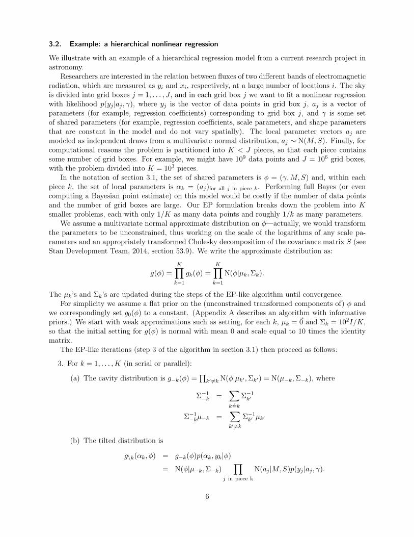
3.2. Example: a hierarchical nonlinear regression

We illustrate with an example of a hierarchical regression model from a current research project inastronomy.

Researchers are interested in the relation between fluxes of two different bands of electromagneticradiation, which are measured as yi and xi, respectively, at a large number of locations i. The skyis divided into grid boxes j = 1, . . . , J , and in each grid box j we want to fit a nonlinear regressionwith likelihood p(yj |aj , γ), where yj is the vector of data points in grid box j, aj is a vector ofparameters (for example, regression coefficients) corresponding to grid box j, and γ is some setof shared parameters (for example, regression coefficients, scale parameters, and shape parametersthat are constant in the model and do not vary spatially). The local parameter vectors aj aremodeled as independent draws from a multivariate normal distribution, aj ∼ N(M,S). Finally, forcomputational reasons the problem is partitioned into K < J pieces, so that each piece containssome number of grid boxes. For example, we might have 109 data points and J = 106 grid boxes,with the problem divided into K = 103 pieces.

In the notation of section 3.1, the set of shared parameters is φ = (γ,M, S) and, within eachpiece k, the set of local parameters is αk = (aj)for all j in piece k. Performing full Bayes (or evencomputing a Bayesian point estimate) on this model would be costly if the number of data pointsand the number of grid boxes are large. Our EP formulation breaks down the problem into Ksmaller problems, each with only 1/K as many data points and roughly 1/k as many parameters.

We assume a multivariate normal approximate distribution on φ—actually, we would transformthe parameters to be unconstrained, thus working on the scale of the logarithms of any scale pa-rameters and an appropriately transformed Cholesky decomposition of the covariance matrix S (seeStan Development Team, 2014, section 53.9). We write the approximate distribution as:

g(φ) =K∏k=1

gk(φ) =K∏k=1

N(φ|µk,Σk).

The µk’s and Σk’s are updated during the steps of the EP-like algorithm until convergence.For simplicity we assume a flat prior on the (unconstrained transformed components of) φ and

we correspondingly set g0(φ) to a constant. (Appendix A describes an algorithm with informativepriors.) We start with weak approximations such as setting, for each k, µk = ~0 and Σk = 102I/K,so that the initial setting for g(φ) is normal with mean 0 and scale equal to 10 times the identitymatrix.

The EP-like iterations (step 3 of the algorithm in section 3.1) then proceed as follows:

3. For k = 1, . . . ,K (in serial or parallel):

(a) The cavity distribution is g−k(φ) =∏k′ 6=k N(φ|µk′ ,Σk′) = N(µ−k,Σ−k), where

Σ−1−k =∑k 6=k

Σ−1k′

Σ−1−kµ−k =∑k′ 6=k

Σ−1k′ µk′

(b) The tilted distribution is

g\k(αk, φ) = g−k(φ)p(αk, yk|φ)

= N(φ|µ−k,Σ−k)∏

j in piece k

N(aj |M,S)p(yj |aj , γ).

6

We can feed this distribution into Stan—it is simply the likelihood for the data in piece j,the priors for the local parameters aj within that piece, and a normal prior on the sharedparameters determined by the cavity distribution—and then we can directly approximateg\k(αk, φ) by a normal distribution (perhaps using a Laplace approximation, perhapsusing some quadrature or importance sampling to better locate the mean and varianceof this tilted distribution) or else simply take some number of posterior draws. Or amore efficient computation may be possible using importance weighting of earlier sets ofsimulations at this node, as we discuss in section 4.6. In any case we can get a normalapproximation to the marginal tilted distribution of the shared parameters, g\k(φ). Callthis approximation, N(µ\k,Σ\k).

(c) The updated approximate site distribution is gnewk = N(µnewk ,Σnewk ), set so gnewk (φ)g−k(φ)

approximates g\k(φ). It would be most natural to do this by matching moments, but it ispossible that the differencing step could result in non-positive-definite covariance matrixΣnewk , so some more complicated step might be needed, as discussed in section 4.7.

(d) We can then perform the appropriate parallel or serial update.

As this example illustrates, the core computation is the inference on the local tilted distributionin step b, and this is where we are taking advantage of the partitioning, both in reduction of thedata and in reduced dimensionality of the computation, as all that is required is inference on theshared parameters φ and the local parameters αk, with the other K − 1 sets of local parametersbeing irrelevant in this step.

3.3. Posterior inference for the approximate joint distribution

Once convergence has been reached for the approximate distribution g(φ), we approximate the jointposterior distribution by g(α1, . . . , αK , φ) = g(φ)

∏Kk=1 p(yk|αk, φ)p(αk|φ). We can work with this

expression in one of two ways, making use of the ability to simulate the model in Stan (or otherwise)in each note.

First, if all that is required are the separate (marginal) posterior distributions for each αkvector, we can take these directly from the simulations or approximations performed in step 3b ofthe algorithm, using the last iteration which can be assumed to be at approximate convergence.This will give simulations of αk or an approximation to p(αk, φ|y).

These separate simulations will not be “in phase,” however, in the sense that different nodeswill be simulating different values of φ. To get draws from the approximate joint distribution of allthe parameters, one can first take some number of draws of the shared parameters φ from the EPapproximation, g(φ), and then, for each draw, run K parallel processes of Stan to perform inferencefor each αk, conditional on the sampled value of φ. This computation is potentially expensive—forexample, to perform it using 100 random draws of φ would require 100 separate Stan runs—but, onthe plus side, each run should converge fast because it is conditional on the hyperparameters of themodel. In addition, it may ultimately be possible to use adiabatic Monte Carlo (Betancourt, 2014)to perform this ensemble of simulations more efficiently.

4. Open issues in implementation

4.1. Algorithmic considerations

Implementing an EP-like algorithm involves several decisions:

7

• Algorithmic blocking. This includes parallelization and partitioning of the likelihood. In thepresent paper we a assume a model with independent data points conditional on its parametersso the likelihood can be factored. The number of subsets K will be driven by computationalconsiderations. IfK is too high, the Gaussian approximation will not be so accurate. However,if K is low, then the computational gains will be small. For large problems it could makesense to choose K iteratively, for example setting to a high value and then decreasing itif the approximation seems too poor. Due to the structure of modern computer memory,the computation using small blocks may get additional speed-up if the most of the memoryaccesses can be made using fast but small cache memory.

• The parametric form of the approximating distributions gk(θ). We will use the multivariatenormal. For simplicity we will also assume that the prior distribution p0(θ) also is multivariatenormal, as is the case in many practical applications, sometimes after proper reparameteriza-tion (such as with constrained parameter spaces). Otherwise, one may treat the prior as anextra site which will also be iteratively approximated by some Gaussian density g0. In thatcase, some extra care is required regarding the initialization of g0.

• The starting distributions gk. We will use a broad but proper distribution factored into Kequal parts, for example setting each gk(θ) = N(0, 1nA

2I), where A is some large value (forexample, if the elements of θ are roughly scaled to be of order 1, we might set A = 10).

• The algorithm to perform inference on the tilted distribution. We will consider three options:deterministic mode-based approximation (in section 4.3), deterministic improvements of mode-based approximations (in section 4.4) and Bayesian simulation (in section 4.5).

• The approximation to the tilted distribution. For mode-based approximations, we can calcu-late the first two moments of the fitted normal or other approximate density; see section 4.4.Or if the tilted distribution is computed by Monte Carlo methods we can compute the firsttwo moments of the simulation, possibly with some regularization if θ is of high dimension;see section 4.5.

• The division by the cavity distribution in step 3c can yield a non-positive-definite variancematrix which would correspond to a meaningless update for gk. We can stabilize this by settingnegative eigenvalues to small positive values or perhaps using some more clever method. Wediscuss this in section 4.7.

In a hierarchical setting, the model can be fit using the nested EP approach (Riihimäki et al.,2013). Assuming that the likelihood term associated with each data partition is approximated witha local Gaussian site function gk(αk, φ), the marginal approximations for φ and all αk could beestimated without forming the potentially high-dimensional joint approximation of all unknowns.At each iteration, first the K local site approximations could be updated in parallel with a fixedmarginal approximation g(φ). Then g(φ) could be refreshed by marginalizing over αk separatelyusing the new site approximations and combining the marginalized site approximations. The parallelEP approximations for each data partition correspond to the inner EP approximations, and inferencefor g(φ) corresponds to the outer EP.

4.2. Approximating the tilted distribution

In standard EP, the tilted distribution approximation in step 3c is done by moment matching prob-lem, which when using the multivariate normal family implies that: one chooses the site gk(θ) so

8

that the first and second moments of gk(θ)g−k(θ) match those of the intractable tilted distributiong\k(θ). When used for Gaussian processes, this approach has the particular advantage that the tilteddistribution g\k(θ) can typically be set up as a univariate distribution over only a single dimensionin θ. This implicit dimension reduction implies that the tilted distribution approximation can beperformed analytically (e.g., Minka, 2001) or relatively quickly using one-dimensional quadrature(e.g., Zoeter and Heskes, 2005). In higher dimensions, quadrature gets computationally more ex-pensive or, with reduced number of evaluation points, the accuracy of the moment computationsgets worse. Seeger (2004) estimated the tilted moments in multiclass classification using multidi-mensional quadratures. Without the possibility of dimension reduction in the more general case,there is no easy way to compute or approximate the integrals to compute the required momentsover θ ∈ Rk. Accordingly, black-box EP would seem to be impossible.

To move towards a black-box EP-like algorithm, we can change this moment matching choice toinstead match the mode or use numerical simulations. The resulting EP-like algorithms criticallypreserve the essential idea that the local pieces of data are analyzed at each step in the contextof a full posterior approximation. These alternative choices for a tilted approximation generallymake EP less stable, and we consider methods for fast and accurate approximations and stabilizingcomputations for EP updates.

Smola et al. (2004) proposed Laplace propagation, where moment-matching is replaced with aLaplace approximation, so that the tilted mean is replaced with the mode of the tilted distributionand the tilted covariance with the inverse Hessian of the log density at the tilted mode. The proofpresented by Smola et al. (2004) suggests that a fixed point of Laplace propagation corresponds toa local mode of the joint model and hence also one possible Laplace approximation. Therefore, withLaplace approximation, a message passing algorithm based on local approximations corresponds tothe global solution. Smola et al. (2004) were able to get useful results with tilted distributions inseveral hundred dimensions. Riihimaki et al. (2013) presented a nested EP method, where momentsof the multivariate tilted distribution are also estimated using EP. For certain model types the innerEP can be computed efficiently.

In this paper, we also consider MCMC computation of the moments, which we suspect willgive inaccurate moment estimates, but may work better than, or as a supplement to, Laplaceapproximation for skewed distributions. We also propose an importance sampling scheme to allowstable estimates based on only a moderate number of simulation draws.

When the moment computations are not accurate, EP may have stability issues, as discussedby Jylänki et al. (2011). Even with one-dimensional tilted distributions, moment computations aremore challenging if the tilted distribution is multimodal or has long tails. Fractional EP (Minka,2004) is an extension of EP which can be used to improve the robustness of the algorithm when theapproximation family is not flexible enough (Minka, 2005) or when the propagation of informationis difficult due to vague prior information (Seeger, 2008). Fractional EP can be viewed as a methodfor minimizing of the α-divergence, with α = 1 corresponding to Kullback-Leibler divergence usedin EP, α = 0 corresponding to the reverse Kullback-Leibler divergence usually used in variationalBayes, and α = 0.5 corresponding to Hellinger distance. Ideas of fractional EP might help tostabilize EP-like algorithms that use approximative moments, as α-divergence with α < 1 is lesssensitive to errors in tails of the approximation.

Section 4.1 details these and other considerations for tilted approximations in our EP-like algo-rithm framework. While the tilted approximation is the key step in any EP-like algorithm, thereare two other canonical issues that must be considered in any EP-like approach: lack of convergenceguarantees and the possible computational instability of the iterations themselves. Section 4.1 alsoconsiders approaches to handle these instabilities.

9

4.3. Normal approximation based on deterministic computations

The simplest EP-like algorithms are deterministic and at each step construct an approximation ofthe tilted distribution around its mode. As Figure 2 illustrates, the tilted distribution can have awell-identified mode even if the factor of the likelihood does not.

The most basic approximation is obtained by, at each step, setting gnew to be the (multivariate)normal distribution centered at the mode of g\k(θ), with covariance matrix equal to the inverseof the negative second derivative matrix of log g\k at the mode. This corresponds to the Laplaceapproximation (Smola et al., 2004). We assume any parameters with restricted range have beentransformed to unrestricted spaces (in Stan, this is done via logarithms of all-positive parameters,logits of interval-constrained parameters, and special transforms for simplex constraints and co-variance matrices; see Stan Development Team, 2014, section 53.9), so the gradient of g\k(θ) willnecessarily be zero at any mode.

The presence of the cavity distribution as a prior (as illustrated in Figure 2) gives two compu-tational advantages to this algorithm. First, we can use the prior mean as a starting point for thealgorithm; second, the use of the prior ensures that at least one mode of the tilted distribution willexist.

4.4. Split-normal and split-t approximations

After computing the mode and curvature at the mode, we can evaluate the tilted distribution ata finite number of points around the mode and use this to construct a better approximation tocapture aspects of asymmetry and long tails in the posterior distribution. Possible approximatefamilies include the multivariate split-normal (Geweke, 1989, Villani and Larsson, 2006), split-t, orwedge-gamma (Gelman et al., 2014) distributions.

We are not talking about changing the family of approximate distributions g—we still wouldkeep these as multivariate normal. Rather, we would use an adaptively-constructed parametric ap-proximation, possibly further improved by importance sampling (Geweke, 1989) or CCD integration(Rue et al., 2009) to get a better approximation to the mean and covariance matrix of the tilteddistribution to use in constructing gk in step 3c of the algorithm.

4.5. Estimating moments using simulation

A different approach is at each step to use simulations (for example, Hamiltonian Monte Carlo usingStan) to approximate the tilted distribution and then use these to set the mean and covariance ofthe approximation in step 3c. As above, the advantage of the EP-like algorithm here is that thecomputation only uses a fraction 1/K of the data, along with a simple multivariate normal prior thatcomes from the cavity distribution. Similar to other inference methods such as stochastic variationalinference (Hoffman et al., 2013) which take steps based on stochastic estimates, EP update stepsneed unbiased estimates. When working with the normal approximation, we then need unbiasedestimates of the mean and precision in ((1)). The variance of the estimates can be reduced whilepreserving unbiasedness by using control variates.

4.6. Reusing simulations with importance weighting

In serial or parallel EP, samples from previous iterations can be reused as starting points for eitherMarkov chains or in importance sampling. We discuss briefly the latter.

Assume we have obtained at iteration t for node k, a set of posterior simulation draws θst,k,s = 1, . . . , St,k from the tilted distribution gt\k, possibly with weights wst,k; take wst,k ≡ 1 for an

10

unweighed sample.To progress to node k + 1, reweight these simulations as: wst,k+1 = wst,kg

t\(k+1)(θ

st,k)/g\k(θ

st,k). If

the effective sample size (ESS) of the new weights,

ESS =

(1S

∑Ss=1w

st,k+1

)21S

∑Ss=1(w

st,k+1)

2,

is large enough, keep this sample, θst,k+1 = θst,k. Otherwise throw it away, simulate new θst+1,k’s fromgt\k+1, and reset the weights wt,k+1 to 1.

This basic approach was used in the EP-ABC algorithm of Barthelmé and Chopin (2014).Elaborations could be considered. Instead of throwing away a sample with too low an ESS, onecould move these through several MCMC steps, in the spirit of sequential Monte Carlo (Del Moralet al., 2006).

Another approach, which can be used in serial or parallel EP, is to use adaptive multiple im-portance sampling (Cornuet et al., 2012), which would make it possible to recycle the simulationsfrom previous iterations.

Even the basic strategy should provide important savings when EP is close to convergence. Thenchanges in the tilted distribution should become small and as result the variance of the importanceweights should be small as well. In practice, this means that the last EP iterations should essentiallycome for free.

4.7. Keeping the covariance matrix positive definite

When working with the normal approximation, step 3c of the EP-like algorithm can be convenientlywritten in terms of the natural parameters of the exponential family:

(Σnewk )−1µnewk = (Σnew)−1µnew − Σ−1−kµ−k

(Σnewk )−1 = (Σnew)−1 − Σ−1−k, (1)

where µnew and Σnew are the approximate mean and covariance matrix of the tilted distribution,and these are being used to determine µnewk and Σnew

k , the mean and variance of the updated sitedistribution gk. The difficulty is that the difference between two positive-definite matrices is notitself necessarily positive definite. There are various tricks in the literature to handle this problem.One idea is to first perform the subtraction in the second line above, then do an eigendecomposition,keeping the eigenvectors of (Σnew

k )−1 but taking any negative eigenvalues and replacing them withsmall positive numbers as in the SoftAbs map of Betancourt (2013). It is not clear whether somesimilar adjustment would be needed for the updating of Σ−1−kµ−k or whether the top line abovewould work as written.

Is it possible to take into account the positive-definiteness restriction in a more principled man-ner? If our measure of the precision matrix of the tilted distribution is noisy (due to Monte Carloerror), it would make sense to include this noise in our inference and estimate µnewk and Σnew

k statis-tically via a measurement-error model. The noisy precision of the tilted distribution is the sum ofthe cavity precision, the precision of the pseudo-observation, and the noise term. Can we infer fromthis better estimate of precision of the pseudo-observation? This itself would be a small Bayesianinference problem but of low enough dimensionality that it should not represent a large part of thecomputation cost compared to the other steps of the algorithm.

An simple and effective alternative is to damp each step so that the resulting cavity covarianceremains positive definite after each update. This does not change the fixed points of the EP

11

algorithm, and adjusts only the step sizes during the iterations. If the updates are done in parallelfashion, it is possible to derive a limit on the damping factor (or step size) so that the cavitycovariances at all sites remain positive definite. The downside is that this requires determiningone eigendecomposition at each site at each parallel update. Based on our experiments, this takesnegligible time compared to the tilted distribution moment computations.

4.8. The computational opportunity of parallel EP-like algorithms

We have claimed that EP-like algorithms offer computational gains for large inference problems bysplitting the data into pieces and performing inference on each of those pieces in parallel, occasionallysharing information between the pieces. Here we detail those benefits specifically.

Consider the simple, non-hierarchical implementation (section 2) with a multivariate normalapproximating family. We assume that we haveK+1 parallel processing units: one central processorthat maintains the global posterior approximation g(θ) and K worker units on which inferencecan be computed on each of the K factors of the likelihood. Furthermore, we assume a networktransmission cost of c per parameter. Let N be the number of data points and let D be the numberof parameters, that is, the length of the vector θ. Finally, we define h(n, d) as the computational costof approximating the tilted distribution (a task which may, for example, be performed by runningMCMC to perform simulations) with n data points and d parameters.

Each step of the algorithm then incurs the following costs:

1. Partitioning. This loading and caching step will in general have immaterial cost.

2. Initialization. The central unit initializes the site approximations gk(θ), which by construc-tion are multivariate normal. In the general case each of theK sites will requireD+D(D+1)/2scalar quantities corresponding to the mean and covariance. Thus the central unit bears theinitialization cost of O(KD2).

3. EP-like iteration. Let m be the number of iterations over all K sites. Empirically m istypically a manageable quantity; however, numerical instabilities tend to increase this number.In parallel EP damped updates are often used to avoid oscillation (van Gerven, 2009).

(a) Computing the cavity distribution. Owing to our multivariate normal approximatingfamily, this step involves only simple rank D matrix operation per site, costing O(D3)(with a small constant; see Cunningham, Hennig, and Lacoste-Julien, 2011). One keychoice is whether to perform this step at the central unit or worker units. If we computethe cavity distributions at each worker unit, the central unit must first transmit the fullposterior to all K worker units, costing O(cND2) for cost c per network operation. Inparallel, the cavity computations then incur total cost ofO(D3). On the other hand, smallD implies central cavity computations are preferred, requiring O(KD3) to construct Kcavity distributions centrally, with a smaller subsequent distribution cost of O(cKD2).Accordingly, the total cost per EP iteration is O(min{cND2 + D3, cKD2 + KD3}).We presume any computation constant is much smaller than the network transmissionconstant c, and thus in the small D regime, this step should be borne by the central unit,a choice strengthened by the presumed burden of step 3c on the worker units.

(b) Forming the tilted distribution. This conceptual step bears no cost.(c) Fitting an updated local approximation gk(θ). We must estimate O(D2) parameters.

More critical in the large data setting is the cost of computing the log-likelihoods. Inthe best case, for example if the likelihoods belong to the same exponential family, we

12

need only calculate a statistic on the data, with cost O(N/K). In some rare cases thedesired moment calculation will be analytically tractable, which results in a minimum costof O(D2 +N/K). Absent analytical moments, we might choose a modal approximation(e.g., Laplace propagation), which may typically incur a O(D3) term. More common still,MCMC or another quadrature approach over theD-dimensional site parameter space willbe more costly still: h(N/K,D) > D2. Furthermore, a more complicated likelihood thanthe exponential family—especially a multimodal p(yk|θ) such as a mixture likelihood—will significantly influence numerical integration. Accordingly, in that common case,this step costs O (h(N/K,D)) � O(D2 + N/K). Critically, our setup parallelizes thiscomputation, and thus the factor K is absent.

(d) Return the updated gk(θ) to the central processor. This cost repeats the cost and con-sideration of Step 3a.

(e) Update the global approximation g(θ). In usual parallel EP, g(θ) is updated once afterall site updates. However, if the cost h of approximating the posterior distribution isvariable across worker units (for example, in an MCMC scheme), the central unit couldupdate g(θ) whenever possible or according to a schedule.

Considering only the dominating terms, across all these steps and the m EP iterations, we havethe total cost of our parallel, EP-like algorithm:

O(m(min{cND2 +D3, cKD2 +KD3}+ h(N/K,D)

)).

This cost contains a term due to Gaussian operations and a term due to parallelized tiltedapproximations. By comparison, consider first the cost of a non-parallel EP-like algorithm:

O(m(ND3 +Nh(N/K,D)

)).

Second, consider the cost of full numerical quadrature with no EP-like partitioning:

O (h(N,D)) .

With these three expressions, we can immediately see the computational benefits of our scheme.In many cases, numerical integration will be by far the most costly operation, and will dependsuperlinearly on its arguments. Thus, our parallel EP-like scheme will dominate. As the total datasize N grows large, our scheme becomes essential. When data is particularly big (e.g. N ≈ 109),our scheme will dominate even in the rare case that h is its minimal O(D2 + N/K) (see step 3cabove).

5. Experiments

5.1. Implementation in Stan

We code our computations in R and Stan. Whether using point estimation (for Laplace approxima-tions) or HMC (for simulations from the tilted distribution), we write a Stan program that includesone portion of the likelihood and an expression for the cavity distribution. We then run this modelrepeatedly with different inputs for each subset k. This ensures that only one part of the likelihoodgets computed at a time by the separate processes, but it does have the cost that separate Stancode is needed to implement the EP computations. In future software development we would liketo be able to take an existing Stan model and merely overlay a factorization so that the EP-likealgorithm could be applied directly to the model.

13

0 1 2 3 4 5 6Mea

n of

par

amat

ers

-4

-2

0

2

4

Iteration0 1 2 3 4 5 6

Std

of p

aram

ater

s

0

0.5

1

1.5

2

Estimated values (+- 3 sigmas)-2 -1 0 1 2

Tru

e va

lues

-2.5

-2

-1.5

-1

-0.5

0

0.5

1

1.5

2

2.5

Figure 4: For simulated logistic regression with 50 parameters and N = 2500 data points in J = 50groups divided into K = 50 pieces: (a) Left plots show the convergence of the EP approximation forthe shared paramaters; (b) Right plot compares the EP inferences for the shared parameters to theirtrue values. Convergence of the algorithm is nearly instantaneous, illustrating the effectiveness ofdispersed computation in this example.

We use Stan to compute step 3a of the EP-like algorithm, the inference for the tilted distributionfor each process. Currently we perform the other steps in Matlab, Python, or R (code will bemade available at https://github.com/gelman/ep-stan). In parallel EP, we pass the normalapproximations gk back and forth between the master node and the K separate nodes.

Currently Stan performs adaptation each time it runs, but the future version should allowrestarting from the previous state, which will speed up computation substantially when the EPalgorithm start to converge. We should also be able to approximate the expectations more efficientlyusing importance sampling.

5.2. Hierarchical logistic regression

We test the algorithm with a simple hierarchical logistic regression,

yi ∼ Bernoulli(αj + βxij)

αj ∼ N(0, τ2),

where β is a vector of common coefficients and each group has own intercept αj with a hierarchicalprior. The data were simulated using xij ∼ N(0, 1), αj ∼ N(0, 22) and β ∼ N(0, 1).

We first perform a simulation experiment with 50 regression predictors, the number of groupsJ = 50, the number of data in each group Nj = 50, and thus a total sample size of N = 2500.For simplicity we partition the data as one piece per group; that is, K = J . The Stan runs had 50warmup and 200 iterations per chain.

If we were to use a simple scheme of data splitting and separate inferences (without using thecavity distribution as an effective prior distribution at each step), the computation would problem-atic: with only 50 data points per group, each of the local posterior distributions would be verywide (as sketched in Figure 1). The EP-like framework, in which at each step the cavity distributionis used as a prior, keeps computations more stable and focused.

14

0 1 2 3 4 5 6Mea

n of

par

amat

ers

-4

-2

0

2

4

Iteration0 1 2 3 4 5 6

Std

of p

aram

ater

s

0

0.5

1

1.5

2

Estimated values (+- 3 sigmas)-2 -1 0 1 2

Tru

e va

lues

-2.5

-2

-1.5

-1

-0.5

0

0.5

1

1.5

2

2.5

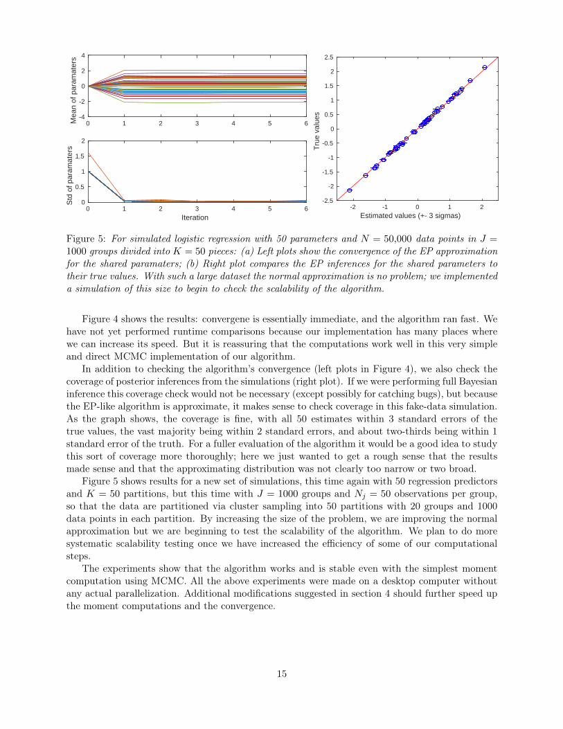
Figure 5: For simulated logistic regression with 50 parameters and N = 50,000 data points in J =1000 groups divided into K = 50 pieces: (a) Left plots show the convergence of the EP approximationfor the shared paramaters; (b) Right plot compares the EP inferences for the shared parameters totheir true values. With such a large dataset the normal approximation is no problem; we implementeda simulation of this size to begin to check the scalability of the algorithm.

Figure 4 shows the results: convergene is essentially immediate, and the algorithm ran fast. Wehave not yet performed runtime comparisons because our implementation has many places wherewe can increase its speed. But it is reassuring that the computations work well in this very simpleand direct MCMC implementation of our algorithm.

In addition to checking the algorithm’s convergence (left plots in Figure 4), we also check thecoverage of posterior inferences from the simulations (right plot). If we were performing full Bayesianinference this coverage check would not be necessary (except possibly for catching bugs), but becausethe EP-like algorithm is approximate, it makes sense to check coverage in this fake-data simulation.As the graph shows, the coverage is fine, with all 50 estimates within 3 standard errors of thetrue values, the vast majority being within 2 standard errors, and about two-thirds being within 1standard error of the truth. For a fuller evaluation of the algorithm it would be a good idea to studythis sort of coverage more thoroughly; here we just wanted to get a rough sense that the resultsmade sense and that the approximating distribution was not clearly too narrow or two broad.

Figure 5 shows results for a new set of simulations, this time again with 50 regression predictorsand K = 50 partitions, but this time with J = 1000 groups and Nj = 50 observations per group,so that the data are partitioned via cluster sampling into 50 partitions with 20 groups and 1000data points in each partition. By increasing the size of the problem, we are improving the normalapproximation but we are beginning to test the scalability of the algorithm. We plan to do moresystematic scalability testing once we have increased the efficiency of some of our computationalsteps.

The experiments show that the algorithm works and is stable even with the simplest momentcomputation using MCMC. All the above experiments were made on a desktop computer withoutany actual parallelization. Additional modifications suggested in section 4 should further speed upthe moment computations and the convergence.

15

6. Discussion

In this paper we have presented a framework for using the EP idea of cavity and tilted distributionsto perform Bayesian inference on partitioned datasets. Particularly in the case of hierarchicalmodels, this structure can allow efficient dispersed computation for big models fit to big data.

6.1. Marginal likelihood

Although not the focus of this work, we mention in passing that EP also offers as no extra cost anapproximation of the marginal likelihood, p(y) =

∫p0(θ)p(y|θ) dθ. This quantity is often used in

model choice.To this end, associate to each approximating site gk a constant Zk, and write the global approx-

imation as:

g(θ) = p0(θ)

K∏k=1

1

Zkgk(θ).

Consider the Gaussian case, for the sake of simplicity, so that gk(θ) = e−12θ′Qkθ+r

′kθ, under

natural parameterization, and denote by Ψ(rk, Qk) the corresponding normalizing constant:

ψ(rk, Qk) =

∫e−

12θ′Qkθ+r

′kθ dθ =

1

2(− log |Qk/2π|+ r′kQkrk).

Simple calculations (Seeger, 2005) then lead to following formula for the update of Zk at site k,

log(Zk) = log(Z\k)−Ψ(r,Q) + Ψ(r−k, Q−k),

where Z\k is the normalizing constant of the tilted distribution g\k, (r,Q) is the natural parameter ofg, r=

∑Kk=1rk, Q=

∑Kk=1Qk, r−k=

∑j 6=i rj , and Q−k=

∑j 6=iQj . In the deterministic approaches we

have discussed for approximating moments of g\k, it is straightforward to obtain an approximationof the normalizing constant; when simulation is used, some extra efforts may be required, as in Chib(1995).

Finally, after completion of EP one should return the following quantity,

K∑k=1

log(Zk) + Ψ(r,Q)−Ψ(r0, Q0),

as the EP approximation of log p(y), where (r0, Q0) is the natural parameter of the prior.

6.2. Different families of approximate distributions

We can place the EP approximation, the tilted distributions, and the target distribution on differentrungs of a ladder:

• g = p0∏Kk=1 gk, the EP approximation;

• For any k, g\k = g pkgk , the tilted distribution;

• For any k1, k2, g\k1,k2 = g pk1pk2gk1gk2, which we might call the tilted2 distribution;

• For any k1, k2, k3, g\k1,k2,k+3 = g pk1pk2pk3gk1gk2gk3, the tilted3 distribution;

• . . .

16

• p =∏Kk=0 pk, the target distribution, which is also the tiltedK distribution.

Instead of independent groups, also tree structures could be used (Minka, 2001). As presented, thegoal of an EP-like algorithm is to determine g. But at each step we get simulations from all theg\k’s, so we could try to combine these inferences in some way (for example, following the ideasof Wang and Dunson, 2013). Even something as simple as mixing the simulation draws from thetilted distribution could be a reasonable improvement on the EP approximation. One could then gofurther, for example at convergence computing simulations from some of the tilted2 distributions.

Another direction is to compare the EP approximation with the tilted distribution, for exam-ple by computing a Kullback-Leibler distance or looking at the distribution of importance weights.Again, we can compute all these densities analytically, we have simulations from the tilted distri-butions, and we can trivially draw simulations from the EP approximation, so all these things arepossible.

6.3. Connections to other approaches

The EP-like algorithm can be combined with other approaches to data partitioning. In the presentpaper we have focused on the construction of the approximate densities gk with the goal of simplymultiplying them together to get the final approximation g = p0

∏Kk=1 gk, but one could instead

think of the cavity distributions g−k at the final iteration as separate priors, and then follow theideas of Wang and Dunson (2013).

Data partitioning is an extremely active research area right now, with several different black-boxalgorithms being proposed by various research groups. We are sure that different methods will bemore effective in different problems. The present paper has two roles: we are presenting a particularblack-box algorithm for distributional approximation, and we are suggesting a general approach toapproaching data partitioning problems. We anticipate that great progress could be made by usingEP ideas to regularize existing algorithms.

References

Ahn, S., Korattikara, A., and Welling, M. (2012). Bayesian posterior sampling via stochastic gra-dient Fisher scoring. In Proceedings of the 29th International Conference on Machine Learning.

Barthelmé, S., and Chopin, N. (2014). Expectation propagation for likelihood-free inference. Jour-nal of the American Statistical Association 109, 315–333.

Betancourt, M. (2013). A general metric for Riemannian manifold Hamiltonian Monte Carlo. http://arxiv.org/abs/1212.4693

Betancourt, M. (2014). Adiabatic Monte Carlo. http://arxiv.org/pdf/1405.3489.pdfChib, S. (1995). Marginal likelihood from the Gibbs output. Journal of the American Statistical

Association 90, 1313–1321.Cornuet, J. M., Marin, J. M., Mira, A., and Robert, C. P. (2012). Adaptive multiple importance

sampling. Scandinavian Journal of Statistics 39, 798–812.Cseke, B., and Heskes, T. (2011). Approximate marginals in latent Gaussian models. Journal of

Machine Learning Research 12, 417–454.Cunningham, J. P., Hennig, P., and Lacoste-Julien, S. (2011). Gaussian probabilities and expecta-

tion propagation. http://arxiv.org/abs/1111.6832Del Moral, P., Doucet, A., and Jasra, A. (2006). Sequential Monte Carlo samplers. Journal of the

Royal Statistical Society B 68, 411–436.

17

Gelman, A., Bois, F. Y., and Jiang, J. (1996). Physiological pharmacokinetic analysis using popu-lation modeling and informative prior distributions. Journal of the American Statistical Asso-ciation 91, 1400–1412.

Gelman, A., Carpenter, B., Betancourt, M., Brubaker, M., and Vehtari, A. (2014). Computationallyefficient maximum likelihood, penalized maximum likelihood, and hierarchical modeling usingStan. Technical report, Department of Statistics, Columbia University.

Gelman, A., Jakulin, A., Pittau, M. G., and Su, Y. S. (2008). A weakly informative default priordistribution for logistic and other regression models. Annals of Applied Statistics 2, 1360–1383.

Gershman, S., Hoffman, M., and Blei, D. (2012). Nonparametric variational inference. In Proceed-ings of the 29th International Conference on Machine Learning.

Geweke, J. (1989). Bayesian inference in econometric models using Monte Carlo integration. Econo-metrica 57, 1317–1339.

Girolami, M., and Zhong, M. (2007). Data integration for classification problems employing Gaus-sian process priors. In Advances in Neural Information Processing Systems 19, ed. B. Scholkopf,J. Platt, and T. Hoffman, 465–472.

Hoffman, M., Blei, D. M., Wang, C., and Paisley, J. (2013). Stochastic variational inference. Journalof Machine Learning Research, 14(1), 1303-1347.

Huang, Z., and Gelman, A. (2005). Sampling for Bayesian computation with large datasets. Tech-nical report, Department of Statistics, Columbia University.

Jylänki, P., Vanhatalo, J., and Vehtari, A. (2011). Robust Gaussian process regression with aStudent-t likelihood. Journal of Machine Learning Research 12, 3227-3257.

Korattikara, A., Chen, Y., and Welling, M. (2013). Austerity in MCMC land: Cutting theMetropolis-Hastings budget. In Proceedings of the 31st International Conference on MachineLearning.

Minka, T. (2001). Expectation propagation for approximate Bayesian inference. In Proceedings ofthe Seventeenth Conference on Uncertainty in Artificial Intelligence, ed. J. Breese and D. Koller,362–369.

Minka, T. (2004). Power EP. Technical report, Microsoft Research, Cambridge.Minka, T. (2005). Divergence measures and message passing. Technical report, Microsoft Research,

Cambridge.Minkser, S., Srivastava, S., Lin, L., and Dunson, D. B. (2014). Robust and scalable Bayes via a

median of subset posterior measures. Technical report, Department of Statistical Science, DukeUniversity. http://arxiv.org/pdf/1403.2660.pdf

Neiswanger, W., Wang, C., and Xing, E. (2013). Asymptotically exact, embarrassingly parallelMCMC. arXiv:1311.4780.

Rasmussen, C. E., and Williams, C. K. I. (2006). Gaussian Processes for Machine Learning. Cam-bridge, Mass.: MIT Press.

Riihimaki, J., Jylänki, P., and Vehtari, A. (2013). Nested expectation propagation for Gaussian pro-cess classification with a multinomial probit likelihood. Journal of Machine Learning Research14, 75–109.

Rue, H., Martino, S., and Chopin, N. (2009). Approximate Bayesian inference for latent Gaussianmodels by using integrated nested Laplace approximations. Journal of the Royal StatisticalSociety B 71, 319–392.

Scott, S. L., Blocker, A. W., Bonassi, F. V., Chipman, H. A., George, E. I., and McCulloch,R. E. (2013). Bayes and big data: The consensus Monte Carlo algorithm. In Bayes 250.

18

http://research.google.com/pubs/pub41849.htmlSeeger, M. (2005). Expectation propagation for exponential families. Technical report, Max Planck

Institute for Biological Cybernetics, Tubingen, Germany.Seeger, M. (2008). Bayesian inference and optimal design for the sparse linear model. Journal of

Machine Learning Research 9, 759–813.Seeger, M., and Jordan, M. (2004). Sparse Gaussian process classification with multiple classes.

Technical report, University of California, Berkeley.Smola, A., Vishwanathan, V., and Eskin, E. (2004). Laplace propagation. In Advances in Neural

Information Processing Systems 16, ed. S. Thrun, L. Saul, and B. Scholkopf.Stan Development Team (2014). Stan modeling language: User’s gude and reference manual, version

2.5.0. http://mc-stan.org/van Gerven, M., Cseke, B., Oostenveld, R., and Heskes, T. (2009). Bayesian source localization

with the multivariate Laplace prior. In Advances in Neural Information Processing Systems 22,ed. Y. Bengio, D. Schuurmans, J. Lafferty, C. K. I. Williams, and A. Culotta, 1901–1909.

Vanhatalo, J., Riihimäki, J., Hartikainen, J., Jylänki, P., Tolvanen, V., and Vehtari, A. (2013).GPstuff: Bayesian modeling with Gaussian processes. Journal of Machine Learning Research14, 1005–1009.

Villani, M., and Larsson, R. (2006). The multivariate split normal distribution and asymmetricprincipal components analysis. Communications in Statistics: Theory and Methods 35, 1123–1140.

Wang, C., and Blei, D. M. (2013). Variational inference in nonconjugate models. Journal of MachineLearning Research 14, 899–925.

Wang, X. (2014). Parallel MCMC via Weirstrass sampler. Xi’an’s Og, 3 Jan. http://xianblog.wordpress.com/2014/01/03/parallel-mcmc-via-weirstrass-sampler-a-reply-by-xiangyu-wang/

Wang, X., and Dunson, D. B. (2013). Parallel MCMC via Weierstrass sampler. http://arxiv.org/pdf/1312.4605v1.pdf

Zoeter, O., and Heskes, T. (2005). Gaussian quadrature based expectation propagation. In Pro-ceedings of the Tenth International Workshop on Artificial Intelligence and Statistics, ed. Z.Ghahramani and R. Cowell, 445–452.

19

A. Distributed parallel algorithms

We have pitched this article at a fairly abstract level because we are interested in the generalidea of using EP-like algorithms to perform parallel Bayesian computation using data splitting.Ultimately, though, these algorithms are motivated by speed and scalability concerns, so we needefficient implementation. In this appendix we go through some of the steps that we went throughto efficiently implement the simulations described in section 5.

A.1. Distributed parallel EP-like algorithm

In this appendix we give a practical algorithm description that is suitable for implementing thegeneral EP-like algorithms of sections 2 and 3 in a numerically stable manner. We assume that theposterior distribution,

p(θ|y) = Z−1K∏k=1

p(yk|θ)p(θ),

is approximated by

g(θ) = Z−1EP

K∏k=1

Z−1k g(θ|rk, Qk)Z−10 g(θ|r0, Q0) = N(θ|µ,Σ),

where the site approximations gk(θ) = Z−1k g(θ|rk, Qk) and the prior p(θ) = N(θ|µ0,Σ0) = Z−10 g(θ|r0, Q0)are written using the following definitions:

g(θ|r,Q) = exp

(−1

2θ′Qθ + r′θ

)Ψ(r,Q) = log

∫g(θ|r,Q)dθ =

1

2

(− log(|Q/2π|) + r′Q−1r

). (2)

The natural parameters and the normalization of the prior p(θ) are given by r0 = Σ−10 µ0, Q0 = Σ−10 ,and logZ0 = Ψ(r0, Q0). The natural exponential parameters of the posterior approximation g(θ)are obtained by multiplying the prior and the site approximations together which gives

Q = Σ−1 =

K∑k=1

Qk +Q0 and r = Σ−1µ =

K∑k=1

rk + r0. (3)

The approximate posterior mean µ = Q−1r and covariance Σ = Q−1 can be computed using aCholesky or eigenvalue decomposition of Q. One possibility to initialize the site approximations isto set them to gk(θ) = 1 by choosing rk = 0 and Qk = 0 for k = 1, . . . ,K, which is equivalent toinitializing g(θ) to the prior, that is, µ = µ0 and Σ = Σ0.

We propose to distribute the cavity and tilted moment computations and the site parameterupdates to K different computing units. The posterior update is done in the central computingnode in a parallel fashion. First, the site updates are initialized to zero as (∆rk = 0,∆Qk = 0)Kk=1

and then the following steps are repeated until convergence:

1. In parallel at each node: Compute the updated site parameters with damping level δ ∈ (0, 1]:

Qnewk = Qk + δ∆Qk

rnewk = rk + δ∆rk.

20

2. At the central node: Compute the natural parameters of g(θ)new as

Qnew =

K∑k=1

Qnewk +Q0

rnew =K∑k=1

rnewk + r0.

3. In parallel at each node: Determine the cavity distributions g−k(θ) = N(µ−k,Σ−k) for allk = 1, . . . ,K:

Q−k = = Qnew − ηQnewk

r−k = = rnew − ηrnewk ,

where η ∈ (0, 1].

4. In parallel at each node: If |Q−k| ≤ 0 for any k, go back to step 1 and decrease δ. Otherwise,accept the new state by setting r = rnew, Q = Qnew, and (Qk = Qnew

k , rk = rnewk )Kk=1 andcontinue to step 5.

5. In parallel at each node: determine the natural parameters r\k = Σ−1\k µ\k and Q\k = Σ−1\k ofthe tilted distribution g\k(zk) using either MCMC or Laplace’s method. The tilted distributionis given by

g\k(θ) = Z−1\k p(yk|θ)ηN(θ|Q−1−kµ−k, Q

−1−k)

∝ p(yk|θ)η exp

(−1

2θ′Q−kθ + r′−kθ

),

which can be efficiently sampled and differentiated using

log g\k(θ) = η log p(yk|θ)−1

2θ′Q−kθ + r′−kθ + const.

Key properties of the different approximation methods:

• MCMC: It is easy to compute µ\k and Σ\k from a set of samples, and Σ\k should besymmetric and positive definite if enough samples are used. However, computing theprecision matrix Q\k = Σ−1\k requires a O(d3) Cholesky or eigenvalue decomposition.Could this be done simultaneously within the SoftAbs stabilization step? In addition,there should be literature on estimating (sparse) precision matrices from samples, whichcould be beneficial with large k.

• Laplace’s method: Gradient-based methods can be used to determine the mode of thetilted distribution efficiently. Once a local mode θ̂ is found, the natural parameters canbe computed as

Q\k = −∇2θ log g\k(θ)|θ=θ̂ = −η∇2

θ log p(yk|θ)|θ=θ̂ +Q−k

r\k = Q\kθ̂.

If θ̂ is a local mode, Q\k should be symmetric and positive definite.

21

6. In parallel at each node: If |Q\k| > 0, compute the undamped site parameter updates resultingfrom the moment consistency conditions Q\k = Q−k + ηQnew

k and r\k = r−k + ηrnewk :

∆Qk = Qnewk −Qk = η−1(Q\k −Q−k)−Qk

∆rk = rnewk − rk = η−1(r\k − r−k)− rk,

If |Q\k| ≤ 0, there are at least two options: discard the update by setting ∆Qk = 0 and∆rk = 0, or use the SoftAbs map to improve the conditioning of Q\k and compute theparameter updates with the modified Q\k.

In the latter approach the natural location parameter of the tilted distribution can be recom-puted as r\k = Q\iµ\k using the original tilted mean µ\k and the modified covariance matrixQ\k, which preserves the tilted mean µ\k but changes tilted covariance estimate Σ\k.

Steps 1–6 are repeated until all the tilted distributions are consistent with the approximate posterior,that is, r = r\k and Q = Q\k for k = 1, . . . ,K. Steps 4 is done to ensure that the posteriorapproximation g(θ) and the cavity distributions g−k(θ) remain well defined at all times. Step 4 ispotentially time consuming because it involves checking the conditioning of all the cavity precisionmatrices {Qk}Kk=1. A cheaper alternative could be to skip the step and apply more damping whichwe expect should work well if the tilted distribution related to the different data pieces are not verydifferent or multimodal.

Advantages of the approach include:

• The central node does not need to compute O(d3) matrix decompositions in step 2. It onlyneeds to sum together the natural site parameters to obtain the posterior approximationin exponential form, and pass this to the individual computing nodes that can make thesubtractions to form the cavity parameters.

• The tilted moments can be determined by sampling directly from the unnormalized tilteddistributions or by using the Laplace’s method. This requires only cheap function and gradientevaluations and can be applied to wide variety of models.

• After convergence the final posterior approximation could be formed by mixing the draws fromthe different tilted distributions because these should be consistent with each other and g(θ).This sample-based approximation could capture also potential skewness in p(θ|y) because itresembles the EP-based marginal improvements described by Cseke and Heskes (2011).

Limitations of the approach include:

• The tilted covariance matrices can be easily computed from samples, but these have to beinverted to obtain the site precision matrices. This inversion could be done by each nodeafter sampling, but if there are more efficient ways to approximate (sparse) precision matricesdirectly from samples, this could be a potential scheme even for large number of unknowns?The algorithm would not require O(d3) matrix decompositions and all the required posteriormarginals could be summarized using samples.

• Estimating the marginal likelihood is more challenging, because determining the normalizationconstants Z\k requires multivariate integrations. For example, annealed importance samplingtype of approaches could be used if marginal likelihood estimates are required.

With the Laplace’s method, approximating Z\k is straightforward by the quality of themarginal likelihood approximation is not likely to very good with skewed posterior distri-butions. The Laplace marginal likelihood estimate is not generally well calibrated with the

22

approximate predictive distributions in terms of hyperparameter estimation. Therefore, itwould make sense to integrate over the hyperparameters within the EP framework.

A.2. Efficient algorithms when dimension reduction is possible

Here we summarize a version of the EP algorithm of section A.1 for the special case in which the non-Gaussian likelihood terms p(yk|θ) depend on θ only through low-dimensional linearly transformedrandom variables,

zk = Ukθ; (4)

that is, p(yk|θ) = p(yk|zk) for each partition k. The posterior distribution is now given by

p(θ|y) = Z−1K∏k=1

p(yk|Ukθ)p(θ),

and we approximate it by

g(θ) = Z−1EP

K∏k=1

Z−1k g(Ukθ|rk, Qk)Z−10 g(θ|r0, Q0) = N(θ|µ,Σ).

The natural parameters of g(θ) are obtained by multiplying the site approximations and the priorwhich gives

Q = Σ−1 =K∑k=1

UkQkU′k +Q0 and r = Σ−1µ =

K∑k=1

Ukrk + r0. (5)

The approximate posterior mean µ = Q−1r and covariance Σ = Q−1 can be computed using aCholesky or eigenvalue decomposition of Q, or a series of K rank-d updates. One possibility is toinitialize the site approximations to gk(θ) = 1 by setting rk = 0 and Qk = 0 for k = 1, . . . ,K, whichis equivalent to initializing g(θ) to the prior, that is, µ = µ0 and Σ = Σ0.

If Uk is a k × d matrix, then the cavity computations and the site parameter updates requireonly rank-d matrix computations, and determining the moments of the kth tilted distribution g\k(θ)requires only d-dimensional numerical integrations. In the following we outline how this algorithmcan be parallelized using m computing units.

We propose to distribute the cavity and tilted moment computations into m different computingunits by dividing the model terms into m non-intersecting subsets Sj so that

⋃mj=1 Sj = {1, . . . ,K}.

The posterior updates are done in the central computing node in a parallel fashion. First, the siteupdates are initialized to zero, (∆rk = 0,∆Qk = 0)Kk=1, and then the following steps are repeateduntil convergence:

1. Distribute parameters (rk, Qk, Uk)i∈Sj and the site parameter updates (∆rk,∆Qk)i=Sj to eachcomputing node j = 1, . . . ,m and compute intermediate natural parameters (Q̃j , r̃j)

mj=1 with

damping level δ ∈ (0, 1]:

(a) Compute the updated site parameters for i ∈ Sj :

Qnewk = Qk + δ∆Qk

rnewk = rk + δ∆rk.

23

(b) Compute the natural parameters of the jth batch:

Q̃j =∑i∈Sj

UkQnewk U ′k

r̃j =∑i∈Sj

Ukrnewk .

2. At the central node, compute the natural parameters of g(θ)new as

Qnew =m∑j=1

Q̃j +Q0

rnew =m∑j=1

r̃j + r0,

and determine the posterior mean µnew = (Qnew)−1rnew and covariance Σnew = (Qnew)−1

using a Cholesky or eigenvalue decomposition.

3. If |Qnew| ≤ 0, go to step 1 and decrease δ. Otherwise, continue to step 4.

4. Distribute µnew, Σnew, and (rnewk , Qnewk , Uk)i∈Sj to each computing node j = 1, . . . ,m, and de-

termine the cavity distributions g−k(zk) = N(m−k, V−k) of the transformed random variableszk = U ′kθ for all i ∈ Sj :

Q−k = V −1−k = V −1k − ηQnewk

r−k = V −1−km−k = V −1k mk − ηrnewk ,

where mk = U ′kµnew and Vk = U ′kΣ

newUk are the moments of the approximate marginaldistribution g(zk) = N(mk, Vk), and η ∈ (0, 1].

Save ck = Ψ(r−k, Q−k)−Ψ(V −1k mk, V−1k ) for computing the marginal likelihood as described

in section 6.1.

5. If |V−k| ≤ 0 for any k, go back to step 1 and decrease δ. Otherwise, accept the new stateby setting r = rnew, Q = Qnew, µ = µnew, Σ = Σnew and (Qk = Qnew

k , rk = rnewk )Kk=1 andcontinue to step 6.

6. Distribute parameters (m−k, V−k, rk, Qk, Uk)i∈Sj to each computing node j = 1, . . . ,m anddetermine the site parameter updates (∆rk,∆Qk)i=Sj using the following steps:

(a) Compute the moments Z\k, m\k = E(zk), and V\k = var(zk) of the tilted distributiong\k(zk) (recall that zk = U ′kθ as defined in (4)) either analytically or using a numericalquadrature depending on the functional form of the exact site term p(yk|U ′θ):

g\k(zk) = Z−1\k p(yk|U′θ)ηN(zk|m−k, V−k) ≈ N(zk|m\k, V\k),

where Z\k =∫p(yk|U ′θ)ηN(zk|m−k, V−k)dzk. Save Z\k for computing the marginal

likelihood as described in section 6.1.

24

(b) If Z\k > 0 and |V\k| > 0, compute the undamped site parameter updates resulting fromthe moment consistency conditions V −1\k = V −1−k +ηQnew

k and V −1\k m\k = V −1−km−k+ηrnewk :

∆Qk = Qnewk −Qk = η−1(V −1\k − V

−1−k )−Qk

∆rk = rnewk − rk = η−1(V −1\k m\k − V−1−km−k)− rk,

If Z\k ≤ 0 or |V\k| ≤ 0, discard the update by setting ∆Qk = 0 and ∆rk = 0.

Steps 1–6 are repeated until all the tilted distributions are consistent with the approximate posterior,that is,mk = m\k and Vk = V\k for k = 1, . . . ,K. Steps 3 and 5 are done to ensure that the posteriorapproximation g(θ) and the cavity distributions g−k(zk) remain well defined at all times. In practicewe expect that these numerical stability checks do not require any additional computations if asuitable damping factor is chosen. An additional approach is to stabilize the computations is toapply more damping to site updates with ∆Qk < 0, because only this kind of precision decreasescan lead to negative cavity distributions.

Without the stability checks, the algorithm can be simplified so that fewer parameter transfersbetween central and the computing nodes are needed per iteration. The algorithm could be furtherstreamlined by doing the posterior updates at steps 1–5 incrementally one batch at a time.

Advantages of the approach include:

• If Uk is a d × 1 matrix, only one-dimensional integrations are required to determine the siteparameters. Furthermore, with certain likelihoods, the conditional moments with respectto some components of zk are analytical which can be used to lower dimensionality of therequired integrations. This goes against the general black-box approach of this paper butcould be relevant for difficult special cases.

• The cavity computations and parameter updates are computationally cheap if d is small. Inaddition, the required computations can be distributed to the different computing nodes in aparallel EP framework.

Limitations of the approach include:

• The model terms need to depend on low-dimensional transformations of the unknowns zk =Ukθ. For example generalized linear models and Gaussian processes fall in to this category.

• Different types of model or likelihood terms require specific implementations. For example,probit and finite Gaussian mixture likelihoods can be handled analytically whereas Poissonand student-t likelihoods require quadratures. For a black-box implementation we might preferto use numerical quadrature for all these problems.

• The central node needs to compute the global posterior covariance at step 2, which scales asO(d3) and can be tedious with a large number of unknowns. Independence assumptions ormultilevel designs as proposed in section 3 can be used to improve the scaling.

A.3. Parallel EP implementation for hierarchical models when approximations are formed alsofor the local parameters

In this section we describe a distributed EP algorithm that uses the hierarchical model structure fromsection 3 for efficient parallel computations in inference problems where a Gaussian approximationis required also for the local parameters. Such cases arise, for example, when certain data pieces

25

share some of the local parameters but we do not wish to form the potentially high dimensionaljoint approximation of φ and all the local parameters.

We assume independent Gaussian priors for φ and α1, . . . , αK and approximate the posteriordistribution

p(α, φ|y) = Z−1N(φ|B−10 b0, B−10 )

K∏k=1

p(yk|αk, φ)N(αk|A−10 a0, A−10 )

by

g(α, φ) = Z−1EPZ−10 g(φ|b0, B0),

K∏k=1

Zkg(αk, φ|rk, Qk)g(αk|a0, A0), (6)

where the site approximations and the prior terms are written using (2), and Z0 is the normalizationterm of the joint prior p(α, φ). To derive the EP updates for the hierarchical model, we divide thesite location vector rk and the site precision matrix Qk to blocks corresponding to αk and φ as

rk =

[akbk

]and Qk =

[Ak CkC ′k Bk

].

The marginal approximation for the shared parameters φ can be obtained by integrating over thelocal parameters αk in the joint approximation (6) as

g(φ) = N(µφ,Σφ) ∝ g(φ|b0, B0)K∏k=1

∫g(αk, φ|rk, Qk)g(αk|a0, A0)dαk ∝ g(φ|b, B),

where the parameters of g(φ) are given by

b = Σ−1φ µφ =

K∑k=1

(bk − C ′k(Ak +A0)

−1(ak + a0))

+ b0

B = Σ−1φ =K∑k=1

(Bk − C ′k(Ak +A0)

−1Ck)

+B0. (7)

In the EP update related to data piece yk we need to consider only the joint marginal approximationof αk and φ, which can be written as

g(αk, φ) ∝ g(αk, φ|rk, Qk)g−k(αk, φ), (8)

where the kth cavity distribution is defined as

g−k(αk, φ) ∝ g(αk|a0, A0)g(φ|b−k, B−k)

with natural parameters

b−k =∑j 6=i

(bj − C ′j(Aj +A0)

−1(aj + a0))

+ b0 = b−(bk − C ′k(Ak +A0)

−1(ak + a0))

B−k =∑j 6=i

(Bj − C ′j(Aj +A0)

−1Cj)

+B0 = B −(Bk − C ′k(Ak +A0)

−1Ck). (9)

The cavity distribution g−k(αk, φ) factorizes between αk and φ, and that the marginal cav-ity of the local parameters αk depends only on the prior p(αk). The dependence on the other

26

local parameters is incorporated in the marginal cavity g−k(φ) ∝ g(φ|b−k, B−k). This propertyresults from the factorized prior between φ and α1, . . . , αK , and it enables computationally efficientlower-dimensional matrix computations. The marginal approximation g(αk) = N(µαk

,Σαk) can be

obtained by integrating over φ in (8), which gives

Σαk=

(A0 +Ak − Ck(B−k +Bk)

−1C ′k)−1

µαk= Σαk

(a0 + ak − Ck(B−k +Bk)

−1(b−k + bk)). (10)

The marginal approximations g(φ) and {g(αk)}Kk=1 can be computed efficiently without actuallyforming the potentially high-dimensional joint approximation g(α1, . . . , αK , φ). After convergence,we can summarize the coefficients and compute the predictions for each group k = 1, . . . ,K usingthe marginal distributions (7) and (10).

Approximations (7) and (10) can be determined by first initializing the site parameters and theparameter updates to zero, that is (ak = 0, bk = 0, Ak = 0, Bk = 0, Ck = 0)Kk=1 and (∆ak = 0,∆bk =0,∆Ak = 0,∆Bk = 0,∆Ck = 0)Kk=1, and then iterating the following steps until convergence:

1. Distribute the current site parameters (ak, Ak, bk, Bk, Ck) together with the parameter updates(∆ak,∆Ak,∆bk,∆Bk,∆Ck) to the corresponding computing node k = 1, . . . ,K, and computenew parameter values with damping level δ ∈ (0, 1]:

anewk = ak + δ∆ak bnewk = ak + δ∆ak

Anewk = Ak + δ∆Ak Bnew

k = Bk + δ∆Bk

Cnewk = Ck + δ∆Ck.

Compute also auxiliary variables Vk = (Anewk +A0)

−1 using, e.g., K parallel Cholesky decom-positions. If |Vk| ≤ 0, i.e., the Cholesky decomposition fails, decrease δ and recompute theupdates. Otherwise, compute auxiliary parameters

b̃k = bnewk − (Cnewk )′Vk(a

newk + a0)

B̃k = Bnewk − (Cnew

k )′VkCnewk .

2. At the central node, compute the natural parameters of g(φ)new = N(µnewφ ,Σnew

φ

)as

bnew = (Σnewφ )−1µnewφ =

K∑k=1

b̃k + b0

Bnew = (Σnewφ )−1 =

K∑k=1

B̃k +B0. (11)

3. Distribute parameters (bnew, Bnew, bnewk , Bnewk ) to the respective computing nodes k = 1, . . . ,K,

and determine the parameters of the cavity distributions:

g−k(αk, φ) = Z−1−kg(αk|a−k, A−k)g(φ|b−k, B−k),

where Z−k = Ψ(a−k, A−k) + Ψ(b−k, B−k) and

a−k = a0 b−k = bnew − b̃kA−k = A0 B−k = Bnew − B̃k.

27

4. If |B−k| ≤ 0 for any k, go back to step 1 and decrease δ. Another option is to skip updatesfor sites {k, |B−k| ≤ 0} but ill-conditioned cavity distributions and approximate covariancematrices may still emerge at subsequent iterations.

Otherwise, accept the new state by setting b = bnew, B = Bnew, and (ak = anewk , Ak =Anewk , bk = bnewk , Bk = Bnew

k , Ck = Cnewk )Kk=1 and continue to the next step. Save the normal-

ization terms logZ−k for computing the marginal likelihood as described in section 6.1.

5. Distribute the parameters (a−k, A−k, b−k, B−k) to the corresponding computing nodes k =1, . . . ,K and determine the site parameter updates by the following steps:

(a) Determine the normalization term Z\k and the moments µ\k = E(αk, φ) and Σ\k =cov(αk, φ) of the tilted distribution g\k(αk, φ) using either an inner EP algorithm orMCMC depending on the functional form of the likelihood term p(yk|αk, φ):

g\k(αk, φ) = Z−1\k p(yk|αk, φ)Z−1−kg(αk|a−k, A−k)g(φ|b−k, B−k) ≈ N(αk, φ|µ\k,Σ\k),

where Z\k =∫p(yk|αk, φ)g−k(αk, φ)dαkdφ. For the site updates only the natural pa-

rameters of the tilted distribution need to be determined:

r\k = Σ−1\k µ\k =

[a\kb\k

]Q\k = Σ−1\k =

[A\k C\k

(C\k)′ B\k

].

(b) If Z\k > 0 and |Q\k| > 0, compute the undamped site parameter updates resulting fromthe moment consistency conditions r\k = r−k + rnewk and Q\k = Q−k +Qnew

k :

∆ak = a\k − a−k − ak ∆bk = b\k − b−k − bk∆Ak = A\k −A−k −Ak ∆Bk = B\k −B−k −Bk∆Ck = C\k − Ck.

Save the following quantity for computing the marginal likelihood as described in section6.1:

ck = logZ\k −Ψ

([a−k + akb−k + bk

],

[A−k +Ak Ck

C ′k B−k +Bk

]).

If Z\k ≤ 0 or |Q\k| ≤ 0, discard the update by setting ∆ak = 0,∆bk = 0,∆Ak =0,∆Bk = 0, and ∆Ck = 0 for that particular data piece k.

A.4. Determining tilted moments using inner EP approximations when dimension reductionis possible

We can use an inner EP algorithm to determine the natural parameters r\k and Q\k of the tilteddistributions g\k(αk, φ) in step 5a of the hierarchical EP algorithm in Appendix A.3, if the like-lihood terms related to each data piece can be factored into simple terms that depend only onlow-dimensional linearly transformed random variables zk,j = Uk,j(αk, φ), that is,

p(yk|αk, φ) =

nk∏j=1

p(yk,j |Uk,j(αk, φ)),

where nk is the number of observations in batch k. The EP algorithm description with dimensionreduction from section A.2 can be readily applied for this purpose. Since the tilted moment ap-proximations in step 5a of the hierarchical algorithm are already run in parallel at the different

28

computing nodes, the parallelization steps in section A.2 can be excluded when used to from theinner EP approximations.

We can also derive closed-form solutions for the parameters (ak, bk, Ak, Bk, Ck)Kk=1 of the ap-

proximation (6) in terms of the site parameters of the inner EP algorithms. First, we write theapproximation to the tilted distributions as

g\k(αk, φ) = Z−1\k Z−1−kp(yk|αk, φ)g(αk|a−k, A−k)g(φ|b−k, B−k)

≈ Z−1\k Z−1−k

nk∏j=1

Zk,jg(Uk,j(αk, φ|r̃k,j , Q̃k,j)g(αk|a−k, A−k)g(φ|b−k, B−k),

where r̃k,j and Q̃k,j are the site parameters of the inner EP approximation. If we write the trans-formation as Uk,j(αk, φ) = uk,jαk + vk,jφ, where Uk,j = (uk,j , vk,j), we can write the outer EPparameters as

ak = a\k − a−k =∑j

uk,j r̃k,j bk = b\k − b−k =∑j

vk,j r̃k,j

Ak = A\k −A−k =∑j

uk,jQ̃k,ju′k,j Bk = B\k −B−k =

∑j

vk,jQ̃k,jv′k,j

Ck = C\k =∑j

uk,jQ̃k,jv′k,j .

For example, in case of a linear model, uk,j are the input variables associated with the local coeffi-cients αk, and vk,j are the input variables corresponding to the shared coefficients φ.

With this representation, we can interpret the hierarchical EP algorithm with K inner EPapproximations also as a single algorithm with site parameters r̃k,j and Q̃k,j that are updated inparallel fashion for K groups of site terms. After each successful update at step 4 we store onlyparameters r̃k,j and Q̃k,j , and we can also equivalently apply damping directly to these parametersat step 1. In fact, it is more efficient to initialize each tilted moment approximation at step 5a tothe inner EP parameters from the previous iteration instead of starting from a zero initialization.This framework is similar to the nested EP algorithm for the multinomial probit model described byRiihimäki et al. (2013). However, if applied to the potentially high-dimensional hierarchical setting,the computationally benefits become more evident compared with the GP classification case studiedin that paper.

29