Expanding the Merit of Utility Maximisation for

Portfolio Choice

Bjorn Hagstromer, Richard G. Anderson, Jane M. Binner,

Thomas Elger, and Birger Nilsson∗

June 21, 2007

Abstract

In the Full-Scale Optimization approach the complete empirical finan-cial return probability distribution is considered, and the utility maximiz-ing solution is found through numerical optimization. Earlier studies haveshown that this approach is useful for investors following non-linear util-ity functions (such as bilinear and S-shaped utility) and choosing betweenhighly non-normally distributed assets, such as hedge funds. We clarifythe role of (mathematical) smoothness and differentiability of the utilityfunction in the relative performance of FSO among a broad class of utilityfunctions.

Using a portfolio choice setting of three common assets (FTSE 100,FTSE 250 and FTSE Emerging Market Index), we identify several utilityfunctions under which Full-Scale Optimization is a substantially betterapproach than the mean variance approach is. Hence, the robustness ofthe technique is illustrated with regard to asset type as well as to utilityfunction specification.

Keywords: Portfolio choice; Utility maximization; Full-Scale Opti-mization, S-shaped utility, bilinear utility.

JEL code: G11

∗Bjorn Hagstromer and Jane M. Binner are from Aston University, UK. Richard G. An-

derson is from Federal Reserve Bank of St. Louis. Thomas Elger and Birger Nilsson are from

Lund University, Sweden. Correspondence to Bjorn Hagstromer: hagstrob@aston.ac.uk or

Richard G. Anderson: Richard.G.Anderson@stls.frb.org . We are grateful for comments and

suggestions by Jim Steeley and Szymon Wlazlowski.

1

1 Introduction

Full-Scale Optimization (FSO) is increasingly attracting the interest of both

portfolio choice researchers and financial industry. In this approach, the portfo-

lio choice is based on direct maximization of a parametric utility function over

the historical returns of the admissible assets (subject to adjustment to reflect

investor expectations). Using numerical optimization to find the optimal port-

folio, it allows for usage of non-linear utility functions. Cremers, Kritzman and

Page (2005), and Adler and Kritzman (2007) apply the model to four different

utility functions, showing that the difference to the mean variance (MV ) model

(Markowitz 1952) can be substantial in hedge fund selection problems when in-

vestors have non-linear utility functions. In this study we apply the FSO model

to a wider selection of utility functions and show that it is useful for other asset

classes than hedge funds.1

For half a century Markowitz’s MV model (1952, 1959) has been the default

model in financial engineering practice, and the benchmark model for new theo-

ries of portfolio choice. In this model, the choice of asset allocations is asserted

to depend solely on the expected return (mean) and risk (variances and covari-

ances) of the admissible assets. This makes the model simple to apply, but it is

based on the assumption that either (1) the return distribution feature spherical

symmetry2, or that (2) investors are indifferent to higher moments and equally

averse to downside and upside risk3.

With respect to returns, ex post financial returns rarely are normal4 - more1The FSO approach is related to the Scenario-Based approach by Koskosidis and Duarte

(1997) and Grinold (1999), and of course to numerous utility maximizing portfolio choicemodels, some of which are referred below.

2This was pointed out by Chamberlain (1983). Below, we refer to such distributions asnormal, even though e.g. the Joint Normal, the Unified and the Binomial distributions alsofeature spherical symmetry.

3These limitations of the MV approach were established at an early point by e.g. To-bin, (1958, 1965), Markowitz (1959), Arrow (1965), Feldstein (1969), Hanoch and Levy,(1969, 1970), Chipman (1973) and Pratt (1976). Rothschild and Stiglitz (1970) showed fromseveral perspectives that the usage of variance as a definition of risk is insufficient. Morerecent assessments of the mean-variance approach include e.g. Epps (1981), Michaud (1989),MacKinlay and Richardson (1991), Chopra and Ziemba (1993), and Clare, Smith and Thomas(1997).

4First recognized by Mandelbrot, (1963), there is now overwhelming evidence available onthe non-normality of returns. This is referred extensively below.

2

often than not, skewness and kurtosis deviate from normality, making the MV

approximation unlikely to select the optimal portfolio when the higher moments

matter to the investor. With respect to utility, an investor indifferent to higher

moments than variance follows a quadratic utility function. While perhaps ac-

ceptable as a local approximation, this function has well-known unattractive

global properties. It has the unrealistic implication that the investor’s absolute

risk aversion is increasing in wealth, so that he at some point of wealth is worse

off as he gets richer.

Markowitz (1987) shows that the difference between quadratic utility and

power utility functions is very small in practice, and several other studies have

come to the same conclusion (e.g. Levy and Markowitz 1979). This conclusion

rests, however, on the existence of continuous higher-order derivatives of the

utility function. In realistic portfolio management situations, investors often

express preferences that do not admit continuous derivatives (Litterman 2003,

Meucci 2005, Ch.2 and Ch.5 respectively). However, the relevance of higher mo-

ments for investment decisions, first pointed out by Levy (1969) and Samuelson

(1970), has caused a plethora of higher moment modifications of the MV ap-

proach to emerge.5

As an alternative solution to the problems of MV analysis, the utility based

approach is well motivated. The problem of non-normal return distribution is

avoided by taking all individual returns into account instead of approximating

the first two moments only, and the utility function can be chosen in accordance

to true investor preferences. The idea of utility maximization as a methodol-

ogy for portfolio optimization problems, based on the utility theory founded

by Von Neumann and Morgenstern (1947), can be traced back at least to To-

bin (1958), and also appeared in the early assessments of the mean-variance

5Lai (1991), Konno, Shirakawa and Yamazaki (1993), Markowitz, Todd, Xu and Yamane(1993), Konno and Suzuki (1995), Chunhachinda, Dandapani, Hamid and Prakash (1997),Leung, Daouk and Chen (2001), and Wang and Xia (2002) suggest models taking skewnessinto account, Lai, Yu and Wang (2006) consider both skewness and kurtosis, Athayde andFlores Jr, (2003, 2004) produce higher moments efficient frontiers, and Britten-Jones (1998)and Harvey, Liechty, Liechty and Muller (2003) approach higher moments with Bayesianmethodologies.

3

approach (e.g. Rothschild and Stiglitz 1971, Levy and Markowitz 1979). In ad-

dition to the common result that the difference to MV was negligible, it was

frequently argued that that utility maximization was computationally too cum-

bersome for the improvement achieved.

Due to its theoretical appeal, however, utility maximization for portfolio

choice has remained present in academia. A relatively recent development of

the method is Full-Scale Optimization. Introduced by Cremers et al. (2005)

(inspired by Grinold 1999), the name captures the fact that the entire historical

return distribution is considered in the optimization problem, rather than sum-

mary statistics thereof. To do this, instead of pursuing an analytical solution,

numerical optimization and dynamic programming is used. This has the second

advantage that the utility function specification is not restricted to mathemati-

cal convenience. Indeed, the function need not exist as a closed form analytical

equation, but rather may be only a convex mapping of wealth and risk into

utility. The computational burden of FSO is even worse than the traditional

utility maximization approaches, but immense technological development dur-

ing the last decades has according to Cremers et al. (2005) and Gourieroux and

Monfort (2005) rendered the computational argument obsolete.6 The econo-

metrics of the FSO approach have recently been examined by Gourieroux and

Monfort (2005), who explore estimator properties and derive a framework for

asset pricing, monitoring constraints and efficiency tests under such estimation.

Cerny (2004) describes how a maximization routine can be programmed.

Assessments of the FSO approach have shown that as long as the utility

function chosen display either continuous derivatives and/or risk aversion that is

a monotone function of wealth, the utility maximizing asset allocations are close

to solutions on the MV efficiency frontier (Grinold 1999, Cremers, Kritzman and

Page 2003, Cremers et al. 2005, Adler and Kritzman 2007). Cremers et al. and

6This argument is often overstated however (Meucci 2005). notes that asset allocation viaFSO is infeasible for more than a small number of assets (his largest example considers 8assets), even when the objective function is convex and the feasible set is the intersection of ahyperplane and a convex set. He recommends conic programming, an approach not pursuedhere.

4

Adler and Kritzman show, however, that the difference between FSO and MV

is substantial when non-linear utility functions, such as bilinear or S-shaped,

are chosen. This is shown in a setting of hedge fund returns, which deviate

substantially from normality7.

We assess the performance of the FSO approach relative to the MV approach

under a spectrum of utility function specifications, wider than previously con-

sidered. Our results illustrate the robustness of Cremers et al. (2005) and Adler

and Kritzman (2007). While the previous studies have been performed on hedge

fund selection problems only, we show that the FSO model is useful even when

very general indices are considered.

This paper is organized as follows. Section 2 gives a detailed account on

the characteristics and preferences of financial return distributions. Section 3

presents the methodology and Section 4 presents the data used for the empirical

comparison of the FSO and MV approaches. The results are presented and

analyzed in Section 5, and section 6 concludes.

2 The nature and preferences of return distri-

butions

Understanding the deviations from normality in financial return distributions

is key in forming an efficient portfolio selection model. We need to understand

both what is causing the deviations, and what preferences investors have for

different distribution characteristics. With that knowledge, appropriate utility

functions can be formed and used for FSO portfolio selection.

2.1 Return distributions

The non-normality of financial asset returns is a problem for mean-variance

analysis as well as for the Capital asset pricing model (Sharpe 1964, Lintner

7It is reasonable to believe that the degree of non-normality influences the difference be-tween FSO and MV positively, but this has yet to be proven.

5

1965, Mossin 1966, Merton 1973a) and the Option pricing model (Black and

Scholes 1973, Merton 1973b). It was discovered long ago that financial asset

price changes formed distributions that are more peaked than samples drawn

from Gaussian distributions. Mandelbrot (1963) credited Mitchell (1915) for

this discovery, and Olivier (1926) and Mills (1927) for the proof of the phe-

nomenon. After Mandelbrot’s article, an extensive literature on the proper

mathematical formulation of financial return distributions emerged, and even-

tually the problem was addressed with techniques such as conditional het-

eroscedasticity models (Engle 1982, Bollerslev 1986), stochastic volatility models

(Clark 1973, Taylor 1982, Taylor 1986), and regime switching models using a

mixture of normal distributions (Goldfeld and Quandt 1973, Hamilton 1989).8

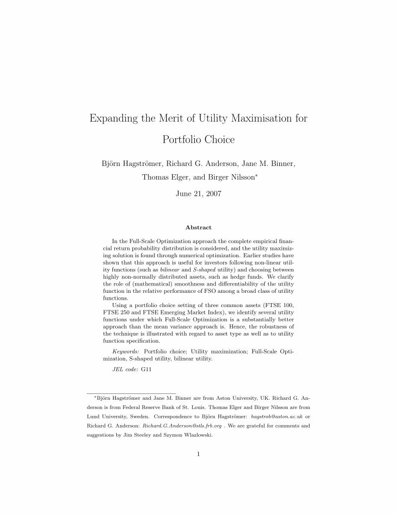
In general, financial assets display leptokurtic return distributions (i.e. dis-

tributions with higher kurtosis than the normal distribution). The logic behind

this fact, pointed out by Clark (1973) and illustrated in Figure 1, is that the

information flows reach the market in a non-linear fashion, causing calm days

when no significant news appear, and chaotic trading on days of path-breaking

news. The calm days form the high peak of the return probability distribution,

and the fat tails are the large price changes due to important news. Non-linear

behavior of investors has also been pointed out as a reason for this pattern

(Aparicio and Estrada 2001), which may be due to uncertainty of information,

or insider trading (Clark). A high level of kurtosis means that the asset has a

high probability of extreme events (Lai et al. 2006). This uncertainty typically

make risk averse investors dislike kurtosis, and such preferences have been the-

oretically proven by Scott and Horvath (1980). Aparicio and Estrada point out

that an investor that mistakenly assumes normality when a return distribution

is leptokurtic, will substantially underestimate the risk of the asset. The non-

normality decreases when long horizon returns are studied, as the news flow to

markets cause less variation in returns when comparing longer periods.

8As the return distribution parameterization is side-stepped by the FSO model, it is notreferred further here, but e.g. Aparicio and Estrada (2001) gives a brief summary of theliterature.

6

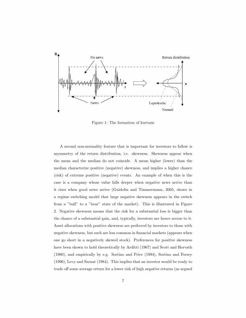
Figure 1: The formation of kurtosis

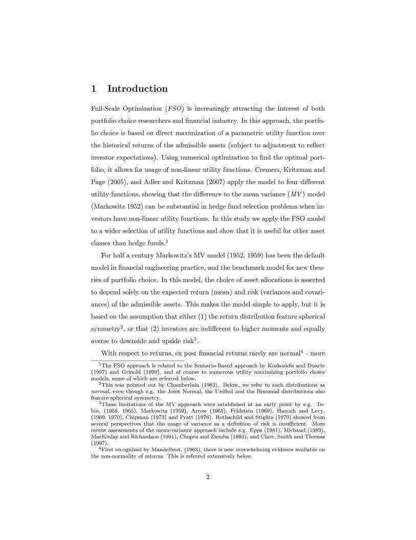
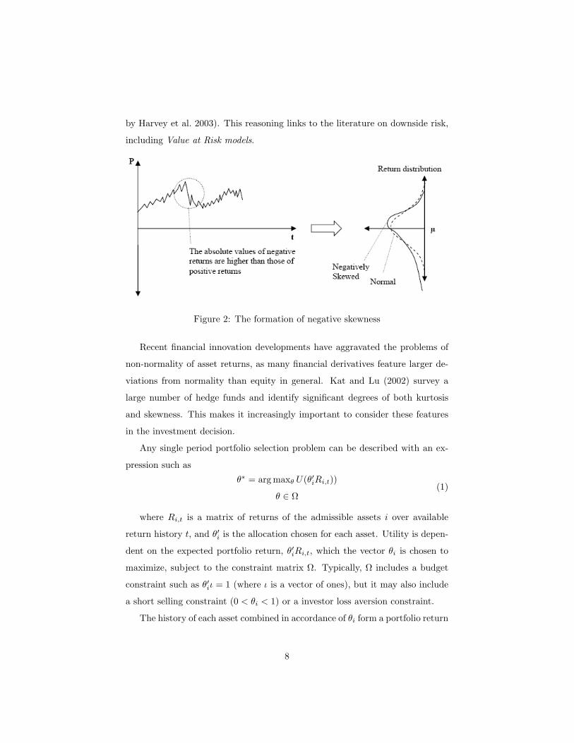
A second non-normality feature that is important for investors to follow is

asymmetry of the return distribution, i.e. skewness. Skewness appear when

the mean and the median do not coincide. A mean higher (lower) than the

median characterize positive (negative) skewness, and implies a higher chance

(risk) of extreme positive (negative) events. An example of when this is the

case is a company whose value falls deeper when negative news arrive than

it rises when good news arrive (Guidolin and Timmermann, 2005, shows in

a regime switching model that large negative skewness appears in the switch

from a ”bull” to a ”bear” state of the market). This is illustrated in Figure

2. Negative skewness means that the risk for a substantial loss is bigger than

the chance of a substantial gain, and, typically, investors are hence averse to it.

Asset allocations with positive skewness are preferred by investors to those with

negative skewness, but such are less common in financial markets (appears when

one go short in a negatively skewed stock). Preferences for positive skewness

have been shown to hold theoretically by Arditti (1967) and Scott and Horvath

(1980), and empirically by e.g. Sortino and Price (1994), Sortino and Forsey

(1996), Levy and Sarnat (1984). This implies that an investor would be ready to

trade off some average return for a lower risk of high negative returns (as argued

7

by Harvey et al. 2003). This reasoning links to the literature on downside risk,

including Value at Risk models.

Figure 2: The formation of negative skewness

Recent financial innovation developments have aggravated the problems of

non-normality of asset returns, as many financial derivatives feature larger de-

viations from normality than equity in general. Kat and Lu (2002) survey a

large number of hedge funds and identify significant degrees of both kurtosis

and skewness. This makes it increasingly important to consider these features

in the investment decision.

Any single period portfolio selection problem can be described with an ex-

pression such as

θ∗ = arg maxθ U(θ′iRi,t))

θ ∈ Ω(1)

where Ri,t is a matrix of returns of the admissible assets i over available

return history t, and θ′i is the allocation chosen for each asset. Utility is depen-

dent on the expected portfolio return, θ′iRi,t, which the vector θi is chosen to

maximize, subject to the constraint matrix Ω. Typically, Ω includes a budget

constraint such as θ′iι = 1 (where ι is a vector of ones), but it may also include

a short selling constraint (0 < θi < 1) or a investor loss aversion constraint.

The history of each asset combined in accordance of θi form a portfolio return

8

probability distribution, Rp. The functional form of the utility function should

mirror the investor’s preferences of the shape of this distribution. Expanding the

utility function in a Taylor series around the mean (µ1) and take expectations on

both sides, as done in Equation 2, yields measures of the investors’ preferences

in terms of the distribution’s moments9. Let Un denote the nth derivative of the

utility function and µi the ith moment of Rp, then (set up in the same fashion

as in Scott and Horvath 1980)

E(U) = U(µ1) +U2(µ1)

2µ2 + Σ∞i=3

µi

i!U i(µ1). (2)

The expression shows that the expected utility equals the utility of the ex-

pected returns, plus the impact on utility of deviations from the expected return.

The influence of each moment on expected utility is weighted by the correspond-

ing order derivative of the utility function. Typically, U2(Rp), for variance is

negative; U3(µ1) for skewness is positive (as discussed above); and U4(µ1) for

kurtosis is negative.10

The MV approach can be viewed in this framework as a utility function with

U1(µ1) = 1, U2(µ1) < 0 (usually referred to as the risk aversion parameter),

and Un(µ1) = 0 for all n > 2.11 This is the quadratic utility function referred

to above, which is an explicit function of the first two moments (U = µ1 − λµ2,

where λ is the risk aversion parameter).12

The explicitness of the MV utility function is not necessary – in the utility

functions to be presented below, the moment preferences are implicit. In princi-

ple there is no limit on the number of moments to take into account, but higher9The term (θ′iRi,t−µ1)U ′(µ1) disappears when taking expectations, as E(θ′iRi,t−µ1) = 0

10The Taylor expansion has frequently been used in the study of investor preferences, seee.g. Arditti (1967) and Markowitz (1987). Hlawitschka (1994) analyzes the methodology.

11In the MV model the covariances of the assets play an important role. These appear inthe utility function when the portfolio return is expressed by its constituents: the individualassets. Accordingly, utility functions with higher moments different from zero will implicitlytake co-skewness and co-kurtosis into account. Co-skewness is a phenomenon extensivelydiscussed by Harvey et al. (2003).

12As referred above, the MV approach is based on either assuming quadratic utility or anormal return distribution. If the latter is assumed, all odd moments (n = 3, 5...) will bezero, and all even moments will be functions of the variance (see Appendix to Chapter 1 inCuthbertson and Nitzsche, 2004).

9

moments than kurtosis (n > 4) have not been considered in the finance litera-

ture, and will not be discussed here. However, according to Scott and Horvath

(1980), most investors have utility functions where moments of odd order (i.e.

n = 1, 3, 5 etc...) have positive signs on its respective derivative, and moments

of even order have negative derivatives.

We note that recently popular utility functions such as linear splines, S-

shaped functions and functions that include limits on decreases in wealth, often

have discontinuous first or second derivatives. These functions are not in the

range of MV analysis.

2.2 Utility functions

The choice of utility function for the estimation is of course crucial for a success-

ful approximation of the optimal portfolio. The utility function must capture

the investor’s preferences as accurately as possible. In the strive for analyti-

cal solutions, mathematical feasibility has traditionally constrained the choice

of utility function. This constraint does not apply for the FSO model, as no

analytical solution is pursued, making the choice truly flexible.

The preferences we want to capture with the utility function have been

described above: favor of mean and skewness and aversion to variance and kur-

tosis.13 The parametric, closed form utility functions that are most common

in the finance literature are the families of exponential and power utility func-

tions. The former is characterized by constant absolute risk aversion (CARA),

and the latter by constant relative risk aversion (CRRA), meaning that risk

aversion varies with wealth level. To consider the investor preferences of skew-

ness and kurtosis in particular, two types of utility functions that have been

suggested are the bilinear and the S-shaped utility function families. Both of

these are characterized by a critical point of investment return, under which

returns are given disproportionally bad utility. The bilinear utility functions13The process of interviewing investors to determine their risk tolerance is discussed by

Litterman (2003,Ch.2) and Meucci (2005, Ch.5). The preferences of actual investors often arenonlinear due to particular biases; modeling these is a topic for future research.

10

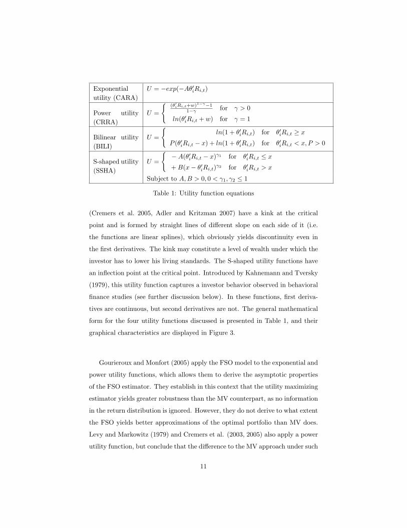
Exponentialutility (CARA)

U = −exp(−Aθ′iRi,t)

Power utility(CRRA)

U =

(θ′iRi,t+w)1−γ−1

1−γ for γ > 0

ln(θ′iRi,t + w) for γ = 1

Bilinear utility(BILI)

U =

ln(1 + θ′iRi,t) for θ′iRi,t ≥ x

P (θ′iRi,t − x) + ln(1 + θ′iRi,t) for θ′iRi,t < x,P > 0

S-shaped utility(SSHA)

U =

−A(θ′iRi,t − x)γ1 for θ′iRi,t ≤ x

+ B(x− θ′iRi,t)γ2 for θ′iRi,t > x

Subject to A,B > 0, 0 < γ1, γ2 ≤ 1

Table 1: Utility function equations

(Cremers et al. 2005, Adler and Kritzman 2007) have a kink at the critical

point and is formed by straight lines of different slope on each side of it (i.e.

the functions are linear splines), which obviously yields discontinuity even in

the first derivatives. The kink may constitute a level of wealth under which the

investor has to lower his living standards. The S-shaped utility functions have

an inflection point at the critical point. Introduced by Kahnemann and Tversky

(1979), this utility function captures a investor behavior observed in behavioral

finance studies (see further discussion below). In these functions, first deriva-

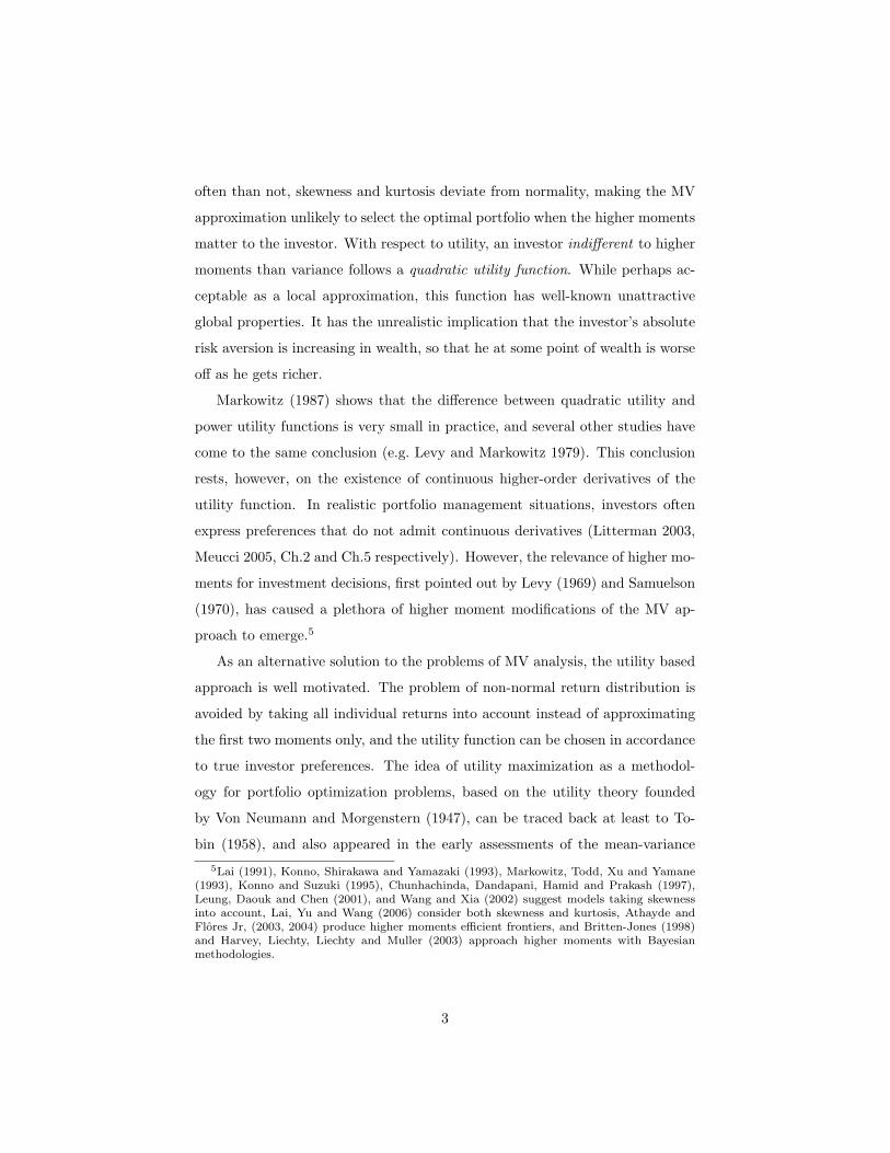
tives are continuous, but second derivatives are not. The general mathematical

form for the four utility functions discussed is presented in Table 1, and their

graphical characteristics are displayed in Figure 3.

Gourieroux and Monfort (2005) apply the FSO model to the exponential and

power utility functions, which allows them to derive the asymptotic properties

of the FSO estimator. They establish in this context that the utility maximizing

estimator yields greater robustness than the MV counterpart, as no information

in the return distribution is ignored. However, they do not derive to what extent

the FSO yields better approximations of the optimal portfolio than MV does.

Levy and Markowitz (1979) and Cremers et al. (2003, 2005) also apply a power

utility function, but conclude that the difference to the MV approach under such

11

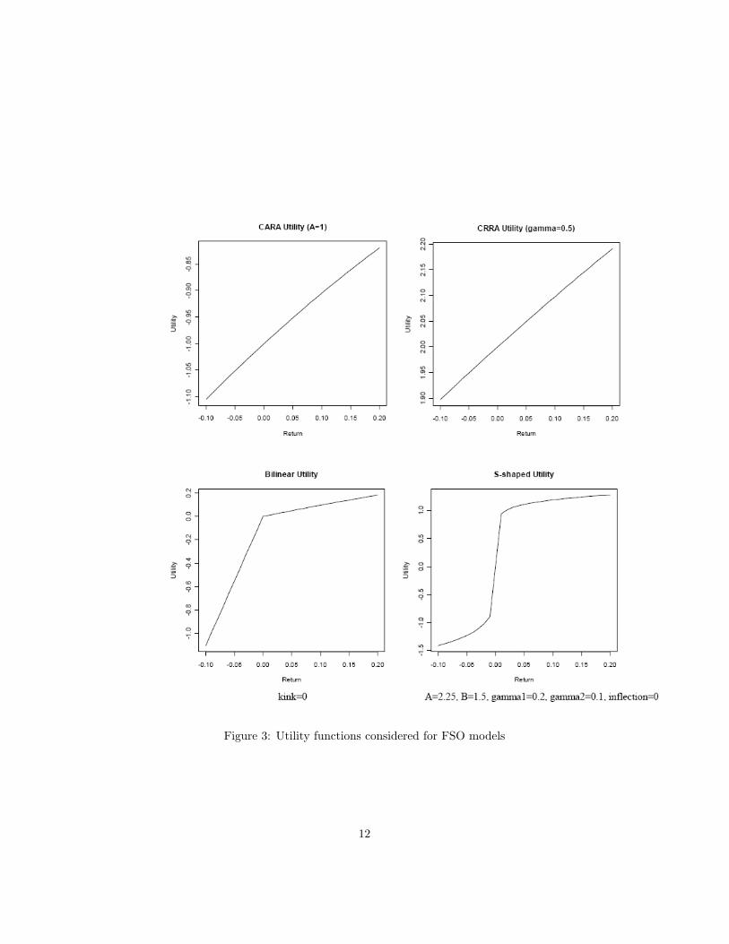
Figure 3: Utility functions considered for FSO models

12

preferences is negligible. In the applications of the bilinear and S-shaped utility

functions, provided by Cremers et al. (2005) and Adler and Kritzman (2007),

substantial differences in performance between FSO and MV approaches are

identified. Such results must however be evaluated in light of how closely the

analytic utility functions describe investor preferences.

The bilinear functions capture a phenomenon that is central in investment

management today: loss aversion. The objective of limiting losses is motivated

by monetary as well as legal purposes. The issue is traditionally treated with

Value-at-Risk models, and can also be incorporated in FSO theory through a

constraint on the maximization problem (as shown by Gourieroux and Monfort

2005). Cremers et al. (2005) show that under bilinear preferences, the resulting

portfolio displays less kurtosis and less down-side risk than the portfolio resulting

from MV analysis, confirming that if loss aversion is desirable to account for,

this is a reasonable way to do it.

The S-shaped utility function is motivated by the fact that it has been shown

in behavior studies that an investor prefers a certain gain to an uncertain gain

with higher expected value, but he also prefers an uncertain loss to a certain loss

with higher expected return. The inflection point is where these certainty pref-

erences changes. The utility function implies high absolute values of marginal

utility close to the inflection point, but low (absolute) marginal utility for higher

(absolute) returns. Hence, this function may make sense in cases when investor

behavior needs to be captured by the model, but it can be questioned whether

it is a utility function investors are striving to fulfill. In the application by

Cremers et al. (2005) it yields a portfolio, which, when compared to the MV

outcome, has fewer negative returns but equal kurtosis.

Utility functions are not all about moments. Further possible extensions in-

clude liquidity preferences, preferences for firm-specific features such as ethical

standards and geographical orientation, and habit formation functions that put

a value to stable consumption patterns. In this study, we limit the investigation

of differences between MV and FSO models to the four utility functions pre-

sented above. This decision, in spite of the plethora of other utility functions, is

13

based on that they have been applied in former FSO performance studies, with

which we intend to compare our results.

3 Methodology

The methodology for comparing the two approaches is to a large extent inspired

by that applied by Cremers et al. (2005), where the performance of the different

approaches is measured in utility.

In the FSO approach the optimal portfolio is found using numerical opti-

mization, often beginning with a grid search. The problem may be thought

of as constructing a matrix Θ containing each possible allocation combination.

The allocation matrix dimension is (n × m), where n is the number of assets

considered, and m is a function of n and a precision parameter p. Each column

of Θ represents one allocation combination vector θ (n×1). To find the optimal

θ, the utility for each theta is evaluated for each asset returns vector Rt, which

contains returns on each asset i at time t, i = 1, 2, ..., n and t = 1, 2, ..., T . Each

of the T − 1 Rt vectors will have dimension (n× 1) and elements Ri,t = Pi,t

Pi,t−1,

where Pi,t is the price of asset i at time t. The θ with highest average utility over

time will be the optimal allocation combination, θFSO. This is shown formally

in Equation 3,

θFSO = maxθa

(T−1

T∑t=1

U(θ′a,iRi,t)

), (3)

where a = 1, 2, ...,m.

The study is performed in a one-period setting – no rebalancing of the port-

folio is considered. As the allocation matrix grows quickly when more assets are

added or the allocation precision p is increased, we use a three asset setting with

p = 1%, and we do not allow for short-selling. This yields an allocation matrix

of dimension (3×5151), which we evaluate over 129 monthly observations. This

rather limited amount of assets and precision is due to the computational bur-

den of the technique. We analyze the full grid of possible allocations – no search

algorithm is applied. As it turns out this level of detail is enough to illustrate the

14

difference between the FSO and MV.14 To illustrate the computational burden

problem, a routine for deriving m is provided in Appendix A.

A common problem in dynamic programming is the choice of starting values.

Litterman (2003) suggests starting the optimization at a vector of ”equilibrium”

returns determined via a CAPM analysis (he labels this the Black-Litterman

approach). Unfortunately, CAPM has been widely rejected in empirical studies

as a description of U.S. asset returns.

For the bilinear and S-shaped utility functions, we also calculate success

rates of the same type as in Cremers et al. (2005)). These are the fraction of

all points in time that yield portfolio returns superior to the investor’s specified

critical level (kink and inflection point respectively).

We apply the same portfolio choice problem to a wide range of utility func-

tions, including the CARA functions, CRRA functions, bilinear functions, and

S-shaped functions. The same utility functions have been investigated before,

but only a few cases of each type. We perform the exercise under several dif-

ferent utility function parameter values, chosen with the intention to cover all

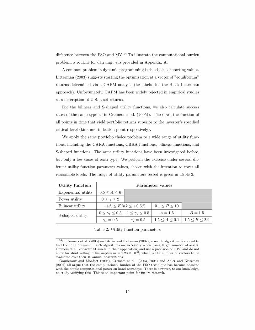
reasonable levels. The range of utility parameters tested is given in Table 2.

Utility function Parameter values

Exponential utility 0.5 ≤ A ≤ 6

Power utility 0 ≤ γ ≤ 2

Bilinear utility −4% ≤ Kink ≤ +0.5% 0.1 ≤ P ≤ 10

S-shaped utility 0 ≤ γ1 ≤ 0.5 1 ≤ γ2 ≤ 0.5 A = 1.5 B = 1.5

γ1 = 0.5 γ2 = 0.5 1.5 ≤ A ≤ 0.1 1.5 ≤ B ≤ 2.9

Table 2: Utility function parameters

14In Cremers et al. (2005) and Adler and Kritzman (2007), a search algorithm is applied tofind the FSO optimum. Such algorithms are necessary when using larger number of assets.Cremers et al. consider 61 assets in their application, and use a precision of 0.1% and do notallow for short selling. This implies m = 7.23 × 1098, which is the number of vectors to beevaluated over their 10 annual observations.

Gourieroux and Monfort (2005), Cremers et al. (2003, 2005) and Adler and Kritzman(2007) all argue that the computational burden of the FSO technique has become obsoletewith the ample computational power on hand nowadays. There is however, to our knowledge,no study verifying this. This is an important point for future research.

15

For the exponential utility function, the only parameter to vary is the level

of risk aversion (A), which we vary between 0.5 and 6. The γ parameter in the

power utility function determines level of risk aversion and how risk aversion

decreases with wealth. As we let it vary between 0 and 2, we include the

special case when the power utility function is logarithmic, which happens when

γ is zero. The higher γ is the lower is the risk aversion. For the bilinear

utility function, we vary the critical point (the kink, varied from -4% to +0.5%)

under which returns are given a disproportionate bad utility. We also vary

the magnitude, P , of this disproportion from 0.1 to 10. In the S-shaped utility

function there are five parameters to vary. We choose to hold the inflection point

fixed at zero, as the idea behind this utility type is loss aversion. The parameters

γ1 and A respectively determine the shape and magnitude of the upside of the

function, whereas γ2 and B determines the downside characteristics in the same

way. The disproportion between gains and losses can be determined either by

the γ parameters or the A and B parameters, or both. We perform one set

of tests where the γ’s vary (γ2 ≥ γ1) and the magnitude parameters are hold

constant and equal, and one set of tests where the gammas are constant and

equal, but where A and B varies (B ≥ A).

4 Data

For the empirical application we use three indices that are published by the

Financial Times, downloaded from Datastream (2006):FTSE 100, FTSE 250,

and FTSE All-World Emerging Market Index (EMI ).15 The FTSE 100 includes

the 100 largest firms on the London Stock Exchange (LSE) and FTSE 250 in-

clude mid-sized firms, i.e. the 250 firms following the hundred largest. The EMI

reflects the performance of mid- and large-sized stocks in emerging markets16.

All series are denoted in British pounds (£). We calculate return series for 10

15The Datastream codes for the indices are FT100GR(PI),FT250GR(PI), and AWA-LEG£(PI).

16For exact definition, see http://www.ftse.com/Indices/FTSE Emerging Markets/Downloads/FTSE Emerging Market Indices.pdf

16

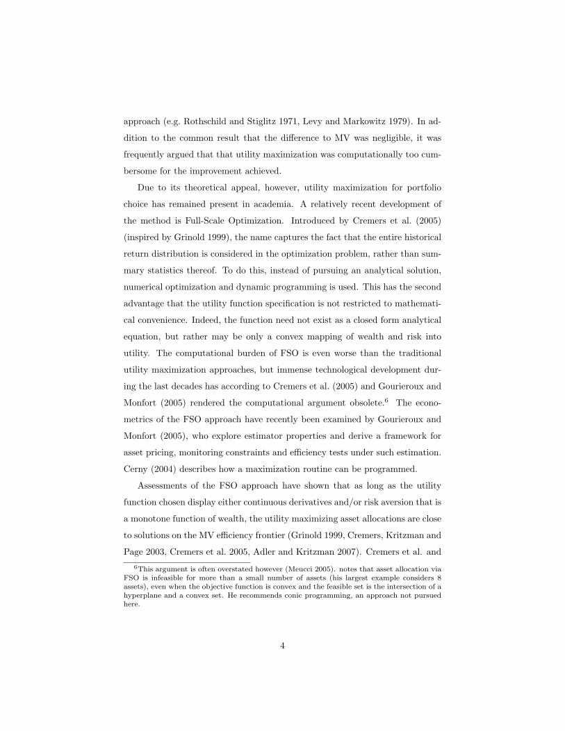
years of monthly observations (25/11 1996 - 27/11 2006), yielding 129 observa-

tions. As shown in Figure 4, the period covers two expansionary periods and

one recession on the UK stock market, whereas the pattern is less clear for the

EMI (likely due to the Russian and Asian crises in the late 1990’s).

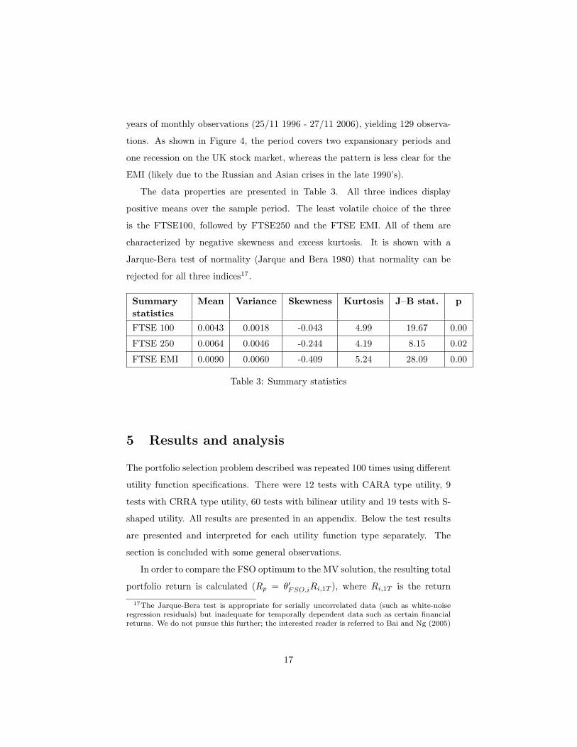
The data properties are presented in Table 3. All three indices display

positive means over the sample period. The least volatile choice of the three

is the FTSE100, followed by FTSE250 and the FTSE EMI. All of them are

characterized by negative skewness and excess kurtosis. It is shown with a

Jarque-Bera test of normality (Jarque and Bera 1980) that normality can be

rejected for all three indices17.

Summarystatistics

Mean Variance Skewness Kurtosis J–B stat. p

FTSE 100 0.0043 0.0018 -0.043 4.99 19.67 0.00

FTSE 250 0.0064 0.0046 -0.244 4.19 8.15 0.02

FTSE EMI 0.0090 0.0060 -0.409 5.24 28.09 0.00

Table 3: Summary statistics

5 Results and analysis

The portfolio selection problem described was repeated 100 times using different

utility function specifications. There were 12 tests with CARA type utility, 9

tests with CRRA type utility, 60 tests with bilinear utility and 19 tests with S-

shaped utility. All results are presented in an appendix. Below the test results

are presented and interpreted for each utility function type separately. The

section is concluded with some general observations.

In order to compare the FSO optimum to the MV solution, the resulting total

portfolio return is calculated (Rp = θ′FSO,iRi,1T ), where Ri,1T is the return

17The Jarque-Bera test is appropriate for serially uncorrelated data (such as white-noiseregression residuals) but inadequate for temporally dependent data such as certain financialreturns. We do not pursue this further; the interested reader is referred to Bai and Ng (2005)

17

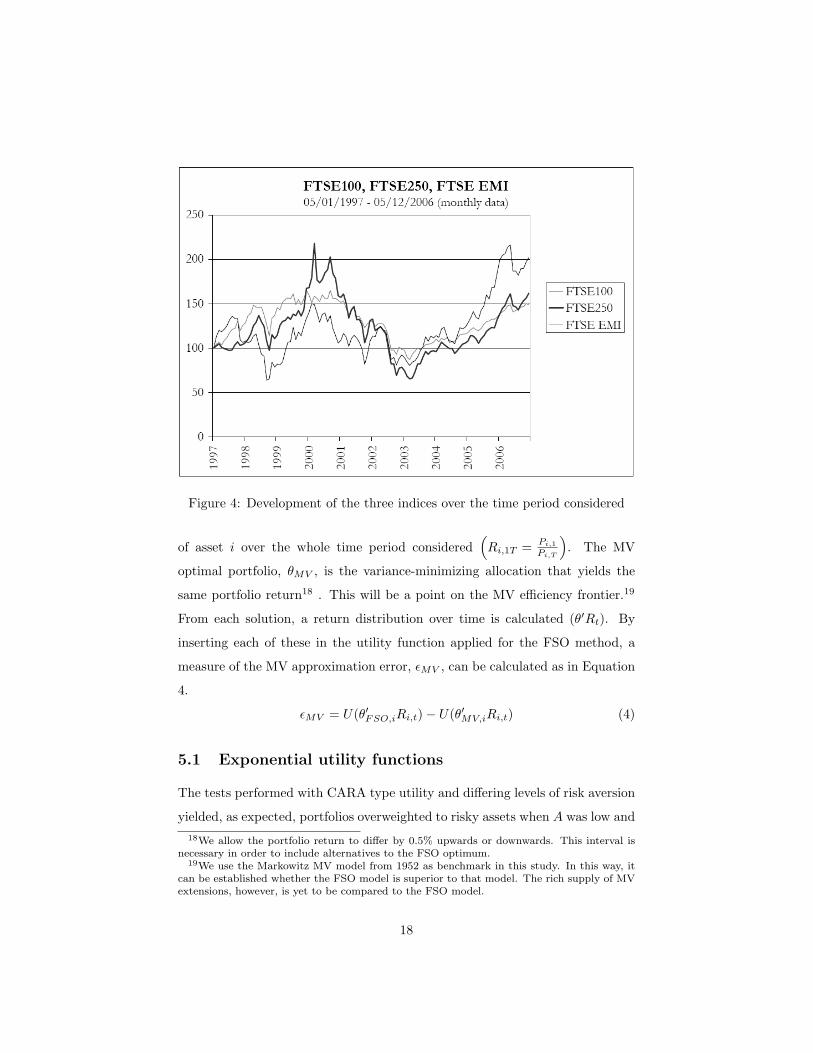
Figure 4: Development of the three indices over the time period considered

of asset i over the whole time period considered(Ri,1T = Pi,1

Pi,T

). The MV

optimal portfolio, θMV , is the variance-minimizing allocation that yields the

same portfolio return18 . This will be a point on the MV efficiency frontier.19

From each solution, a return distribution over time is calculated (θ′Rt). By

inserting each of these in the utility function applied for the FSO method, a

measure of the MV approximation error, εMV , can be calculated as in Equation

4.

εMV = U(θ′FSO,iRi,t)− U(θ′MV,iRi,t) (4)

5.1 Exponential utility functions

The tests performed with CARA type utility and differing levels of risk aversion

yielded, as expected, portfolios overweighted to risky assets when A was low and18We allow the portfolio return to differ by 0.5% upwards or downwards. This interval is

necessary in order to include alternatives to the FSO optimum.19We use the Markowitz MV model from 1952 as benchmark in this study. In this way, it

can be established whether the FSO model is superior to that model. The rich supply of MVextensions, however, is yet to be compared to the FSO model.

18

underweighted to less risky assets when A was high. Portfolio allocations chosen

on the mean variance efficiency frontier yielded small differences in portfolio re-

turn - only in one case did the difference exceed 0.005%. These results conform

well to those of Cremers et al. (2005) and Adler and Kritzman (2007), showing

that portfolio allocations chosen by the utility maximizing approaches consti-

tute very small improvements relative to the MV approach, when the investor’s

utility is well described by the CARA or CRRA utility functions.

5.2 Power utility functions

Portfolio allocations based on power utility functions were selected with 9 dif-

ferent levels of gamma, implying different levels of risk aversion and change of

risk aversion as wealth grows. For low levels of gamma, the allocations are

overweighted to the risky assets, gradually changing to the non-risky assets as

gamma grows. The special case when gamma is 1 yields a non-diversified port-

folio allocating all money to the EMI - the most risky asset. This is logical,

because the size of the returns in this case is all that matters (U = ln(R)). The

differences in utility to the corresponding MV portfolio allocations are small,

reaching at most 0.02%. These small differences conform to the previous studies.

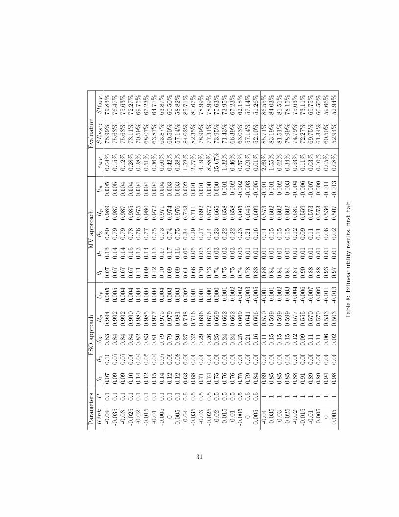
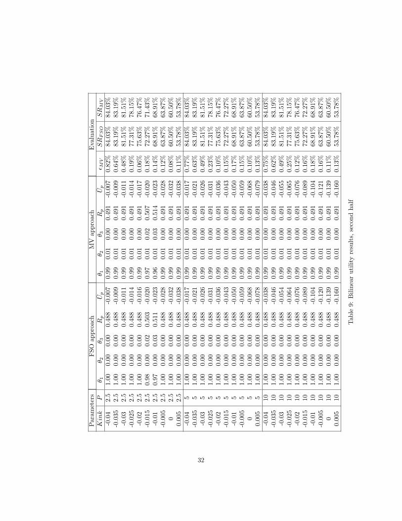
5.3 Bilinear utility functions

The tests on bilinear utility functions (i.e. linear splines) were performed with

the kink (knot) at different levels and various penalties (P ) on sub-kink returns.

Each kink value was tested for 10 different penalty levels. Referring back to the

utility function specification in Table 1, it is seen that the penalty is subtracted

from a fixed level of utility on all returns. For the lowest penalty, 0.1, well-

diversified portfolio allocations are chosen, but higher penalty cause less risky

assets to be preferred. For penalty levels above one, the deviations from the

safest portfolio possible (100% on the least risky asset) are small. This occurs

when the incentive to avoid returns less than those associated with the kink

dominates other investor incentives, such as maximizing returns or minimizing

19

risk by diversification.

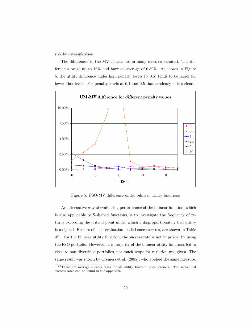
The differences to the MV choices are in many cases substantial. The dif-

ferences range up to 16% and have an average of 0.89%. As shown in Figure

5, the utility difference under high penalty levels (> 0.5) tends to be larger for

lower kink levels. For penalty levels at 0.1 and 0.5 that tendency is less clear.

Figure 5: FSO-MV difference under bilinear utility functions

An alternative way of evaluating performance of the bilinear function, which

is also applicable to S-shaped functions, is to investigate the frequency of re-

turns exceeding the critical point under which a disproportionately bad utility

is assigned. Results of such evaluation, called success rates, are shown in Table

420. For the bilinear utility function, the success rate is not improved by using

the FSO portfolio. However, as a majority of the bilinear utility functions led to

close to non-diversified portfolios, not much scope for variation was given. The

same result was shown by Cremers et al. (2005), who applied the same measure.

20These are average success rates for all utility function specifications. The individualsuccess rates can be found in the appendix.

20

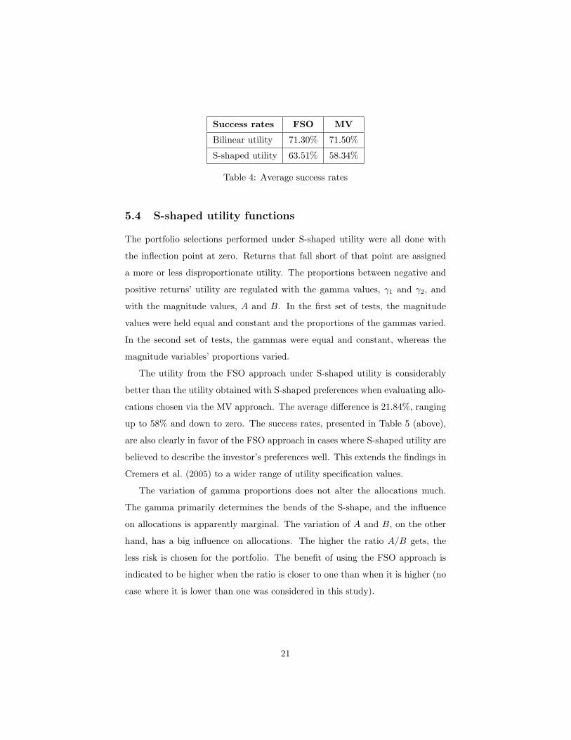
Success rates FSO MV

Bilinear utility 71.30% 71.50%

S-shaped utility 63.51% 58.34%

Table 4: Average success rates

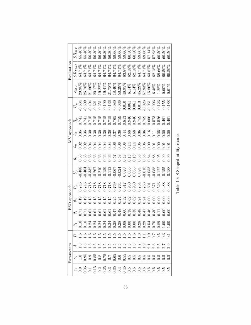
5.4 S-shaped utility functions

The portfolio selections performed under S-shaped utility were all done with

the inflection point at zero. Returns that fall short of that point are assigned

a more or less disproportionate utility. The proportions between negative and

positive returns’ utility are regulated with the gamma values, γ1 and γ2, and

with the magnitude values, A and B. In the first set of tests, the magnitude

values were held equal and constant and the proportions of the gammas varied.

In the second set of tests, the gammas were equal and constant, whereas the

magnitude variables’ proportions varied.

The utility from the FSO approach under S-shaped utility is considerably

better than the utility obtained with S-shaped preferences when evaluating allo-

cations chosen via the MV approach. The average difference is 21.84%, ranging

up to 58% and down to zero. The success rates, presented in Table 5 (above),

are also clearly in favor of the FSO approach in cases where S-shaped utility are

believed to describe the investor’s preferences well. This extends the findings in

Cremers et al. (2005) to a wider range of utility specification values.

The variation of gamma proportions does not alter the allocations much.

The gamma primarily determines the bends of the S-shape, and the influence

on allocations is apparently marginal. The variation of A and B, on the other

hand, has a big influence on allocations. The higher the ratio A/B gets, the

less risk is chosen for the portfolio. The benefit of using the FSO approach is

indicated to be higher when the ratio is closer to one than when it is higher (no

case where it is lower than one was considered in this study).

21

5.5 General results

This empirical application illustrates the robustness of the finding of Cremers

et al. (2005) and Adler and Kritzman (2007) that the FSO approach in general

is useful when investor preferences are well described by non-mathematically

smooth utility functions, including the bilinear and S-shaped utility functions. If

investor preferences are well described by a power or exponential utility function,

there is little benefit of using the FSO rather than the MV approach. This is

shown in a more general framework than in preceding studies, investigating a

wide scope of utility function parameter level.

The fact that these results appear in an application of such general indices

as the FTSE 100 and FTSE 250 increases the scope of the FSO applicability.

It has earlier only been shown that the FSO is useful in allocation problems

involving hedge funds.

6 Conclusions

The empirical application of this study constitutes the widest FSO-MV compar-

ison to date with respect to utility functions. The results extend earlier findings

by Cremers et al. (2005) and Adler and Kritzman (2007), establishing the ro-

bustness of those studies’ results. Our results also emphasize the important

role of the mathematical smoothness of the utility function. The FSO method-

ology is useful when investor utility function features a threshold, such as in

the bilinear and the S-shaped utility functions. For traditional utility functions

(exponential and power utility) the MV approach yields similar results. The

main empirical contribution of this study is that the scope of the FSO applica-

bility is extended to more general stocks, as the sample used features the FTSE

100 and FTSE 250 with limited non-normality in the return distributions (in

previous studies the methodology has been proven useful only in hedge fund

applications).

Future research on the Full-Scale Optimization methodology needs to focus

22

on the choice of utility function and its parameters. These are crucial for an

adequate portfolio optimization. The scope of the usefulness of the FSO ap-

proach also deserves more attention. Furthermore, the computational burden

of the numerical optimization needed for the FSO model needs to be clarified

before the simplicity of the mean variance approach can be deemed an obsolete

argument.

References

Adler, T. and Kritzman, M.: 2007, Mean–variance versus full–scale optimisa-tion: In and out of sample, forthcoming in Journal of Asset Management7(5), 302–311.

Aparicio, F. and Estrada, J.: 2001, Empirical distributions of stock returns:European securities markets, 1990-95, The European Journal of Finance7(1), 1–21.

Arditti, F.: 1967, Risk and the required return on equity, The Journal of Fi-nance 22(1), 19–36.

Arrow, K.: 1965, Aspects of a theory of risk bearing.” yrjo jahnsson lectures,helsinki. reprinted in essays in the theory of risk bearing 1971.

Athayde, G. and Flores Jr, R.: 2003, Incorporating skewness and kurtosis inportfolio optimization, in S. Satchell and A. Scowcroft (eds), Advancesin Portfolio Construction and Implementation, Butterworth-Heinemann,pp. 243–57.

Athayde, G. and Flores, R.: 2004, Finding a maximum skewness portfolio–ageneral solution to three-moments portfolio choice, Journal of EconomicDynamics and Control 28(7), 1335–1352.

Bai, J. and Ng, S.: 2005, Tests for skewness, kurtosis, and normality for timeseries data, Journal of Business & Economic Statistics 23(1), 49–61.

Black, F. and Scholes, M.: 1973, The pricing of options and corporate liabilities,The Journal of Political Economy 81(3), 637–654.

Bollerslev, T.: 1986, Generalized autoregressive conditional heterocedasticity,Journal of Econometrics 31, 307–327.

Britten-Jones, M.: 1998, Portfolio optimization and bayesian regression, LondonBusiness School .

23

Cerny, A.: 2004, Mathematical techniques in finance, Princeton University PressPrinceton, NJ.

Chamberlain, G.: 1983, Characterization of the distributions that imply mean-variance utility functions., Journal of Economic Theory 29(1), 185–201.

Chipman, J.: 1973, The ordering of portfolios in terms of mean and variance,The Review of Economic Studies 40(2), 167–190.

Chopra, V. and Ziemba, W.: 1993, The effect of errors in means, variances, andcovariances on optimal portfolio choice, Journal of Portfolio Management19(2), 6–11.

Chunhachinda, P., Dandapani, K., Hamid, S. and Prakash, A.: 1997, Portfolioselection and skewness: Evidence from international stock markets, Journalof Banking and Finance 21(2), 143–167.

Clare, A., Smith, P. and Thomas, S.: 1997, Uk stock returns and robust tests ofmean variance efficiency, Journal of Banking and Finance 21(5), 641–660.

Clark, P.: 1973, A subordinated stochastic process model with finite variancefor speculative prices, Econometrica 41(1), 135–155.

Cremers, J. H., Kritzman, M. and Page, S.: 2005, Optimal hedge fund alloca-tions, Journal of Portfolio Management 31(3), 70–81.

Cremers, J., Kritzman, M. and Page, S.: 2003, Portfolio formation with highermoments and plausible utility, Technical report, Revere Street WorkingPaper Series, Financial Economics 272-12.

Cuthbertson, K. and Nitzsche, D.: 2004, Quantitative Financial Economics:Stocks, Bonds and Foreign Exchange, Wiley.

Engle, R.: 1982, Autoregressive conditional heteroscedasticity with estimates ofthe variance of united kingdom inflation, Econometrica 50(4), 987–1008.

Epps, T.: 1981, Necessary and sufficient conditions for the mean-variance port-folio model with constant risk aversion, The Journal of Financial andQuantitative Analysis 16(2), 169–176.

Feldstein, M.: 1969, Mean-variance analysis in the theory of liquidity preferenceand portfolio selection, The Review of Economic Studies 36(1), 5–12.

Goldfeld, S. and Quandt, R.: 1973, A markov model for switching regressions,Journal of Econometrics 1(1).

Gourieroux, C. and Monfort, A.: 2005, The econometrics of efficient portfolios,Journal of Empirical Finance 12, 1–41.

Grinold, R.: 1999, Mean-variance and scenario-based approaches to portfolioselection, Journal of Portfolio Management 25(2), 10–22.

24

Guidolin, M. and Timmermann, A.: 2005, International asset allocation underregime switching, skew and kurtosis preferences, Federal Reserve Bank ofSt. Louis Working Paper (2005–034B).

Hamilton, J.: 1989, A new approach to the economic analysis of nonstationarytime series and the business cycle, Econometrica 57(2), 357–384.

Hanoch, G. and Levy, H.: 1969, The efficiency analysis of choices involving risk,The Review of Economic Studies 36(3), 335–346.

Hanoch, G. and Levy, H.: 1970, Efficient portfolio selection with quadratic andcubic utility, The Journal of Business 43(2), 181–189.

Harvey, C., Liechty, J., Liechty, M. and Muller, P.: 2003, Portfolio selectionwith higher moments, Technical report, Working Paper, Duke University.

Hlawitschka, W.: 1994, The empirical nature of taylor-series approximations toexpected utility, The American Economic Review 84(3), 713–719.

Jarque, C. and Bera, A.: 1980, Efficient tests for normality, homoscedas-ticity and serial independence of regression residuals, Economics Letters6(3), 255–259.

Kahnemann, D. and Tversky, A.: 1979, Prospect theory: An analysis of decisionunder risk, Econometrica 47(2), 263–291.

Kat, H. and Lu, S.: 2002, An excursion into the statistical properties of hedgefunds, Technical report, Working Paper, ISMA Center, University of Read-ing, UK.

Konno, H., Shirakawa, H. and Yamazaki, H.: 1993, A mean-absolute deviation-skewness portfolio optimization model, Annals of Operations Research45(1), 205–220.

Konno, H. and Suzuki, K.: 1995, A mean-variance-skewness portfolio op-timization model, Journal of the Operations Research Society of Japan38(2), 173–187.

Koskosidis, Y. and Duarte, A.: 1997, A scenario-based approach to active assetallocation, Journal of Portfolio Management 23(2), 74–85.

Lai, K., Yu, L. and Wang, S.: 2006, Mean-variance-skewness-kurtosis-based portfolio optimization, Proceedings of the First International Multi-Symposiums on Computer and Computational Sciences (IMSCCS’06).

Lai, T.: 1991, Portfolio selection with skewness: A multiple-objective approach,Review of Quantitative Finance and Accounting 1(3), 293–305.

Leung, M., Daouk, H. and Chen, A.: 2001, Using investment portfolio return tocombine forecasts: A multiobjective approach, European Journal of Oper-ational Research 134(1), 84–102.

25

Levy, H.: 1969, A utility function depending on the first three moments, TheJournal of Finance 24(4), 715–719.

Levy, H. and Markowitz, H.: 1979, Approximating expected utility by a functionof mean and variance, The American Economic Review 69(3), 308–317.

Levy, H. and Sarnat, M.: 1984, Portfolio and Investment Selection: Theory andPractice, Prentice/Hall International.

Lintner, J.: 1965, Security prices, risk, and maximal gains from diversification,The Journal of Finance 20(4), 587–615.

Litterman, R.: 2003, Modern Investment Management: An Equilibrium Ap-proach, John Wiley & Sons Inc.

MacKinlay, A. and Richardson, M.: 1991, Using generalized method of momentsto test mean-variance efficiency, The Journal of Finance 46(2), 511–527.

Mandelbrot, B.: 1963, The variation of certain speculative prices, The Journalof Business 36(4), 394–419.

Markowitz, H.: 1952, Portfolio selection, The Journal of Finance 7(1), 77–91.

Markowitz, H.: 1959, Portfolio selection: Efficient diversification of investments,Yale UP, New Haven .

Markowitz, H.: 1987, Mean-variance analysis in portfolio choice and capitalmarkets, Basil Blackwell.

Markowitz, H., Todd, P., Xu, G. and Yamane, Y.: 1993, Computation of mean-semivariance efficient sets by the critical line algorithm, Annals of Opera-tions Research 45(1), 307–317.

Merton, R.: 1973a, An intertemporal capital asset pricing model, Econometrica41(5), 867–887.

Merton, R.: 1973b, Theory of rational option pricing, The Bell Journal of Eco-nomics and Management Science 4(1), 141–183.

Meucci, A.: 2005, Risk and Asset Allocation, Springer.

Michaud, R.: 1989, The markowitz optimization enigma: Is optimized optimal,Financial Analysts Journal 45(1), 31–42.

Mossin, J.: 1966, Equilibrium in a capital asset market, Econometrica34(4), 768–783.

Pratt, J.: 1976, Risk aversion in the small and in the large, Econometrica44(2), 420–420.

Rothschild, M. and Stiglitz, J.: 1970, Increasing risk: I. a definition, Journal ofEconomic Theory 2(3), 225–243.

26

Rothschild, M. and Stiglitz, J.: 1971, Increasing risk ii: Its economic conse-quences, Journal of Economic Theory 3(1), 66–84.

Samuelson, P.: 1970, The fundamental approximation theorem of portfolio anal-ysis in terms of means, variances and higher moments, The Review of Eco-nomic Studies 37(4), 537–542.

Scott, R. and Horvath, P.: 1980, On the direction of preference for moments ofhigher order than the variance, The Journal of Finance 35(4), 915–919.

Sharpe, W.: 1964, Capital asset prices: A theory of market equilibrium underconditions of risk, The Journal of Finance 19(3), 425–442.

Sortino, F. and Forsey, H.: 1996, On the use and misuse of downside risk,Journal of Portfolio Management 22(2), 35–42.

Sortino, F. and Price, L.: 1994, Performance measurement in a downside riskframework, Journal of Investing 3(3), 50–58.

Taylor, S.: 1982, Financial returns modeled by the product of two stochasticprocesses-a study of the daily sugar prices 1961-75, Time Series Analysis:Theory and Practice 1, 203–226.

Taylor, S.: 1986, Modelling financial time series, Wiley New York.

Tobin, J.: 1958, Liquidity preference as behavior towards risk, The Review ofEconomic Studies 25(2), 65–86.

Tobin, J.: 1965, The theory of portfolio selection, in F. Hahn and F. Brechling(eds), The Theory of Interest Rates, London: MaxMillan and Co., Ltd.

Von Neumann, J. and Morgenstern, O.: 1947, Theory of games and economicbehavior, Princeton University Press.

Wang, S. and Xia, Y.: 2002, Portfolio selection and asset pricing, Springer NewYork.

27

Appendix A: The dimensions of the allocation

matrix Θ

The asset allocation matrix contains all possible combinations of allocations of

n assets (n = 1, 2, ), with precision p (0 < p < 100% such that 1/p is an integer).

The matrix dimension is (n×m). This appendix studies how m, the number of

allocation combinations, is related to n and p when no short selling is allowed21.

The simplest possible Θ matrix is the one asset case, when the only option

is to invest 100% of the portfolio in that asset and m = 1. When going from

one asset to the two asset case, the width growth factor, gi will always be

(g1 = m2 = p−1 + 1). When 10% precision is used, the two asset case has a

matrix width m2 = 11, as illustrated in Figure 6.

1.0 0.9 0.8 0.7 0.6 0.5 0.4 0.3 0.2 0.1 0.00.0 0.1 0.2 0.3 0.4 0.5 0.6 0.7 0.8 0.9 1.0

Figure 6: Example of Θ matrix (n = 2; p = 10%)

Adding another asset to this example yields m3 = 66, implying a growth

factor g2 = 6. If precision is increased to p = 1% (note that increased precision

implies that p declines) we will get matrices of the width m2 = 101 and m3 =

5151, implying growth rates of g1 = 101 and g2 = 51. At this stage the following

tendencies can be noted about the function m = f(n, p):

• The width is growing in both asset number and precision: δmδn > 1, δm

δp >

−1

• The growth rate decreases with the number of assets: δgn

δn < 0

• The growth rate decreases with precision: δgn

δp > 0

We have not been able to mathematically prove a formula for m, but by

observation on how the Θ matrix grows, we have derived a three-step formula

that holds exactly for all matrices we have generated. These steps are given in21If no constraint on short selling is set, m will be infinite.

28

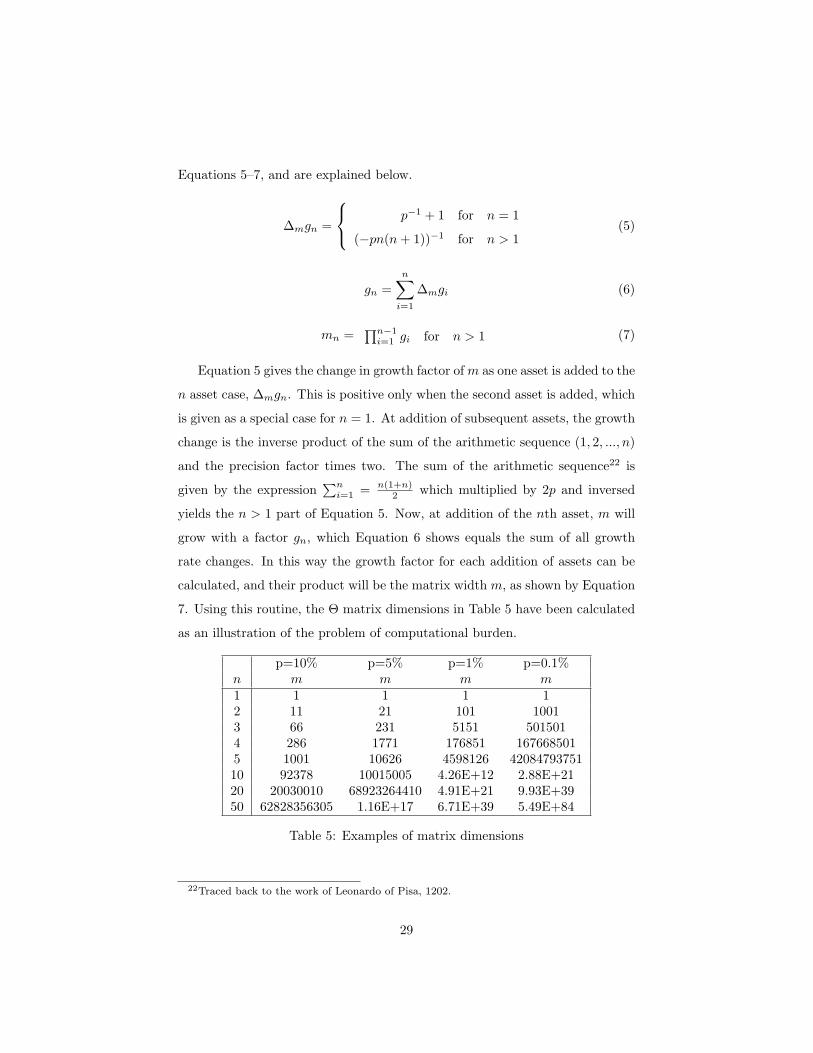
Equations 5–7, and are explained below.

∆mgn =

p−1 + 1 for n = 1

(−pn(n + 1))−1 for n > 1(5)

gn =n∑

i=1

∆mgi (6)

mn =∏n−1

i=1 gi for n > 1 (7)

Equation 5 gives the change in growth factor of m as one asset is added to the

n asset case, ∆mgn. This is positive only when the second asset is added, which

is given as a special case for n = 1. At addition of subsequent assets, the growth

change is the inverse product of the sum of the arithmetic sequence (1, 2, ..., n)

and the precision factor times two. The sum of the arithmetic sequence22 is

given by the expression∑n

i=1 = n(1+n)2 which multiplied by 2p and inversed

yields the n > 1 part of Equation 5. Now, at addition of the nth asset, m will

grow with a factor gn, which Equation 6 shows equals the sum of all growth

rate changes. In this way the growth factor for each addition of assets can be

calculated, and their product will be the matrix width m, as shown by Equation

7. Using this routine, the Θ matrix dimensions in Table 5 have been calculated

as an illustration of the problem of computational burden.

p=10% p=5% p=1% p=0.1%n m m m m1 1 1 1 12 11 21 101 10013 66 231 5151 5015014 286 1771 176851 1676685015 1001 10626 4598126 4208479375110 92378 10015005 4.26E+12 2.88E+2120 20030010 68923264410 4.91E+21 9.93E+3950 62828356305 1.16E+17 6.71E+39 5.49E+84

Table 5: Examples of matrix dimensions

22Traced back to the work of Leonardo of Pisa, 1202.

29

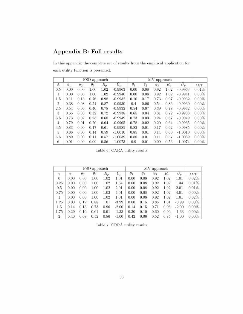
Appendix B: Full results

In this appendix the complete set of results from the empirical application for

each utility function is presented.

FSO approach MV approachA θ1 θ2 θ3 Rp Up θ1 θ2 θ3 Rp Up εMV

0.5 0.00 0.00 1.00 1.02 -0.9963 0.00 0.08 0.92 1.02 -0.9963 0.01%1 0.00 0.00 1.00 1.02 -0.9940 0.00 0.08 0.92 1.02 -0.9941 0.00%

1.5 0.11 0.13 0.76 0.98 -0.9932 0.10 0.17 0.73 0.97 -0.9932 0.00%2 0.38 0.08 0.54 0.87 -0.9930 0.4 0.06 0.54 0.86 -0.9930 0.00%

2.5 0.54 0.06 0.40 0.78 -0.9932 0.54 0.07 0.39 0.78 -0.9932 0.00%3 0.65 0.03 0.32 0.72 -0.9938 0.65 0.04 0.31 0.72 -0.9938 0.00%

3.5 0.73 0.02 0.25 0.68 -0.9949 0.73 0.03 0.24 0.67 -0.9949 0.00%4 0.79 0.01 0.20 0.64 -0.9965 0.78 0.02 0.20 0.64 -0.9965 0.00%

4.5 0.83 0.00 0.17 0.61 -0.9985 0.82 0.01 0.17 0.62 -0.9985 0.00%5 0.86 0.00 0.14 0.59 -1.0010 0.85 0.01 0.14 0.60 -1.0010 0.00%

5.5 0.89 0.00 0.11 0.57 -1.0039 0.88 0.01 0.11 0.57 -1.0039 0.00%6 0.91 0.00 0.09 0.56 -1.0073 0.9 0.01 0.09 0.56 -1.0074 0.00%

Table 6: CARA utility results

FSO approach MV approachγ θ1 θ2 θ3 Rp Up θ1 θ2 θ3 Rp Up εMV

0 0.00 0.00 1.00 1.02 1.01 0.00 0.08 0.92 1.02 1.01 0.02%0.25 0.00 0.00 1.00 1.02 1.34 0.00 0.08 0.92 1.02 1.34 0.01%0.5 0.00 0.00 1.00 1.02 2.01 0.00 0.08 0.92 1.02 2.01 0.01%0.75 0.00 0.00 1.00 1.02 4.01 0.00 0.08 0.92 1.02 4.01 0.00%1 0.00 0.00 1.00 1.02 1.01 0.00 0.08 0.92 1.02 1.01 0.02%

1.25 0.00 0.12 0.88 1.01 -3.99 0.00 0.15 0.85 1.01 -3.99 0.00%1.5 0.14 0.13 0.73 0.96 -2.00 0.14 0.15 0.71 0.96 -2.00 0.00%1.75 0.29 0.10 0.61 0.91 -1.33 0.30 0.10 0.60 0.90 -1.33 0.00%2 0.40 0.08 0.52 0.86 -1.00 0.42 0.06 0.52 0.85 -1.00 0.00%

Table 7: CRRA utility results

30

Par

amet

ers

FSO

appr

oach

MV

appr

oach

Eva

luat

ion

Kin

kP

θ 1θ 2

θ 3R

pU

pθ 1

θ 2θ 3

Rp

Up

ε MV

SR

FS

OS

RM

V

-0.0

40.

10.

070.

100.

830.

994

0.00

50.

070.

130.

800.

989

0.00

50.

04%

78.9

9%79

.83%

-0.0

350.

10.

090.

070.

840.

992

0.00

50.

070.

140.

790.

987

0.00

50.

15%

75.6

3%76

.47%

-0.0

30.

10.

090.

070.

840.

992

0.00

40.

070.

140.

790.

987

0.00

40.

12%

75.6

3%75

.63%

-0.0

250.

10.

100.

060.

840.

990

0.00

40.

070.

150.

780.

985

0.00

40.

28%

73.1

1%72

.27%

-0.0

20.

10.

140.

040.

820.

980

0.00

40.

110.

130.

760.

975

0.00

40.

28%

70.5

9%69

.75%

-0.0

150.

10.

120.

050.

830.

985

0.00

40.

090.

140.

770.

980

0.00

40.

51%

68.0

7%67

.23%

-0.0

10.

10.

150.

040.

810.

977

0.00

40.

120.

130.

750.

972

0.00

40.

36%

63.8

7%64

.71%

-0.0

050.

10.

140.

070.

790.

975

0.00

40.

100.

170.

730.

971

0.00

40.

60%

63.8

7%63

.87%

00.

10.

120.

090.

790.

979

0.00

30.

090.

170.

740.

974

0.00

30.

42%

60.5

0%60

.50%

0.00

50.

10.

120.

080.

800.

981

0.00

30.

090.

160.

750.

976

0.00

30.

28%

57.1

4%58

.82%

-0.0

40.

50.

630.

000.

370.

748

0.00

20.

610.

050.

340.

743

0.00

21.

52%

84.0

3%85

.71%

-0.0

350.

50.

680.

000.

320.

716

0.00

10.

660.

050.

290.

711

0.00

12.

77%

82.3

5%80

.67%

-0.0

30.

50.

710.

000.

290.

696

0.00

10.

700.

030.

270.

692

0.00

14.

19%

78.9

9%78

.99%

-0.0

250.

50.

740.

000.

260.

676

0.00

00.

730.

030.

240.

672

0.00

08.

88%

77.3

1%78

.99%

-0.0

20.

50.

750.

000.

250.

669

0.00

00.

740.

030.

230.

665

0.00

015

.67%

73.9

5%75

.63%

-0.0

150.

50.

760.

000.

240.

662

-0.0

010.

750.

030.

220.

658

-0.0

011.

32%

71.4

3%73

.95%

-0.0

10.

50.

760.

000.

240.

662

-0.0

020.

750.

030.

220.

658

-0.0

020.

46%

66.3

9%67

.23%

-0.0

050.

50.

750.

000.

250.

669

-0.0

020.

740.

030.

230.

665

-0.0

020.

57%

63.0

3%62

.18%

00.

50.

790.

000.

210.

641

-0.0

030.

780.

010.

210.

645

-0.0

030.

09%

57.1

4%57

.14%

0.00

50.

50.

840.

000.

160.

606

-0.0

050.

830.

010.

160.

609

-0.0

050.

01%

52.1

0%51

.26%

-0.0

41

0.89

0.00

0.11

0.57

0-0

.001

0.88

0.01

0.11

0.57

3-0

.001

2.69

%85

.71%

86.5

5%-0

.035

10.

850.

000.

150.

599

-0.0

010.

840.

010.

150.

602

-0.0

011.

55%

83.1

9%84

.03%

-0.0

31

0.85

0.00

0.15

0.59

9-0

.002

0.84

0.01

0.15

0.60

2-0

.002

0.62

%81

.51%

81.5

1%-0

.025

10.

850.

000.

150.

599

-0.0

030.

840.

010.

150.

602

-0.0

030.

34%

78.9

9%78

.15%

-0.0

21

0.88

0.00

0.12

0.57

7-0

.004

0.87

0.01

0.12

0.58

1-0

.004

0.53

%74

.79%

75.6

3%-0

.015

10.

910.

000.

090.

555

-0.0

060.

900.

010.

090.

559

-0.0

060.

11%

72.2

7%73

.11%

-0.0

11

0.89

0.00

0.11

0.57

0-0

.007

0.88

0.01

0.11

0.57

3-0

.007

0.03

%69

.75%

69.7

5%-0

.005

10.

890.

000.

110.

570

-0.0

090.

880.

010.

110.

573

-0.0

090.

10%

61.3

4%60

.50%

01

0.94

0.00

0.06

0.53

3-0

.011

0.93

0.01

0.06

0.53

6-0

.011

0.05

%60

.50%

59.6

6%0.

005

10.

980.

000.

020.

503

-0.0

130.

970.

010.

020.

507

-0.0

130.

08%

52.9

4%52

.94%

Tab

le8:

Bili

near

utili

tyre

sult

s,fir

stha

lf

31

Par

amet

ers

FSO

appr

oach

MV

appr

oach

Eva

luat

ion

Kin

kP

θ 1θ 2

θ 3R

pU

pθ 1

θ 2θ 3

Rp

Up

ε MV

SR

FS

OS

RM

V

-0.0

42.

51.

000.

000.

000.

488

-0.0

070.

990.

010.

000.

491

-0.0

070.

82%

84.0

3%84

.03%

-0.0

352.

51.

000.

000.

000.

488

-0.0

090.

990.

010.

000.

491

-0.0

090.

64%

83.1

9%83

.19%

-0.0

32.

51.

000.

000.

000.

488

-0.0

110.

990.

010.

000.

491

-0.0

110.

48%

81.5

1%81

.51%

-0.0

252.

51.

000.

000.

000.

488

-0.0

140.

990.

010.

000.

491

-0.0

140.

19%

77.3

1%78

.15%

-0.0

22.

51.

000.

000.

000.

488

-0.0

160.

990.

010.

000.

491

-0.0

170.

06%

75.6

3%76

.47%

-0.0

152.

50.

980.

000.

020.

503

-0.0

200.

970.

010.

020.

507

-0.0

200.

18%

72.2

7%71

.43%

-0.0

12.

50.

970.

000.

030.

511

-0.0

230.

960.

010.

030.

514

-0.0

230.

14%

68.9

1%68

.91%

-0.0

052.

51.

000.

000.

000.

488

-0.0

280.

990.

010.

000.

491

-0.0

280.

12%

63.8

7%63

.87%

02.

51.

000.

000.

000.

488

-0.0

320.

990.

010.

000.

491

-0.0

320.

08%

60.5

0%60

.50%

0.00

52.

51.

000.

000.

000.

488

-0.0

380.

990.

010.

000.

491

-0.0

380.

11%

53.7

8%53

.78%

-0.0

45

1.00

0.00

0.00

0.48

8-0

.017

0.99

0.01

0.00

0.49

1-0

.017

0.77

%84

.03%

84.0

3%-0

.035

51.

000.

000.

000.

488

-0.0

210.

990.

010.

000.

491

-0.0

210.

63%

83.1

9%83

.19%

-0.0

35

1.00

0.00

0.00

0.48

8-0

.026

0.99

0.01

0.00

0.49

1-0

.026

0.49

%81

.51%

81.5

1%-0

.025

51.

000.

000.

000.

488

-0.0

310.

990.

010.

000.

491

-0.0

310.

23%

77.3

1%78

.15%

-0.0

25

1.00

0.00

0.00

0.48

8-0

.036

0.99

0.01

0.00

0.49

1-0

.036

0.10

%75

.63%

76.4

7%-0

.015

51.

000.

000.

000.

488

-0.0

430.

990.

010.

000.

491

-0.0

430.

15%

72.2

7%72

.27%

-0.0

15

1.00

0.00

0.00

0.48

8-0

.050

0.99

0.01

0.00

0.49

1-0

.050

0.17

%68

.91%

68.9

1%-0

.005

51.

000.

000.

000.

488

-0.0

590.

990.

010.

000.

491

-0.0

590.

15%

63.8

7%63

.87%

05

1.00

0.00

0.00

0.48

8-0

.068

0.99

0.01

0.00

0.49

1-0

.068

0.10

%60

.50%

60.5

0%0.

005

51.

000.

000.

000.

488

-0.0

780.

990.

010.

000.

491

-0.0

790.

13%

53.7

8%53

.78%

-0.0

410

1.00

0.00

0.00

0.48

8-0

.038

0.99

0.01

0.00

0.49

1-0

.038

0.75

%84

.03%

84.0

3%-0

.035

101.

000.

000.

000.

488

-0.0

460.

990.

010.

000.

491

-0.0

460.

62%

83.1

9%83

.19%

-0.0

310

1.00

0.00

0.00

0.48

8-0

.054

0.99

0.01

0.00

0.49

1-0

.055

0.49

%81

.51%

81.5

1%-0

.025

101.

000.

000.

000.

488

-0.0

640.

990.

010.

000.

491

-0.0

650.

25%

77.3

1%78

.15%

-0.0

210

1.00

0.00

0.00

0.48

8-0

.076

0.99

0.01

0.00

0.49

1-0

.076

0.12

%75

.63%

76.4

7%-0

.015

101.

000.

000.

000.

488

-0.0

890.

990.

010.

000.

491

-0.0

890.

16%

72.2

7%72

.27%

-0.0

110

1.00

0.00

0.00

0.48

8-0

.104

0.99

0.01

0.00

0.49

1-0

.104

0.18

%68

.91%

68.9

1%-0

.005

101.

000.

000.

000.

488

-0.1

200.

990.

010.

000.

491

-0.1

210.

16%

63.8

7%63

.87%

010

1.00

0.00

0.00

0.48

8-0

.139

0.99

0.01

0.00

0.49

1-0

.139

0.11

%60

.50%

60.5

0%0.

005

101.

000.

000.

000.

488

-0.1

600.

990.

010.

000.

491

-0.1

600.

13%

53.7

8%53

.78%

Tab

le9:

Bili

near

utili

tyre

sult

s,se

cond

half

32

Par

amet

ers

FSO

appr

oach

MV

appr

oach

Eva

luat

ion

γ1

γ2

AB

θ 1θ 2

θ 3R

pU

pθ 1

θ 2θ 3

Rp

Up

ε MV

SR

FS

OS

RM

V

0.0

1.0

1.5

1.5

0.10

0.71

0.19

0.74

6-0

.488

0.63

0.02

0.35

0.74

1-0

.634

29.9

5%64

.71%

55.4

6%0.

050.

951.

51.

50.

100.

710.

190.

746

-0.4

040.

630.

020.

350.

741

-0.5

0925

.78%

64.7

1%55

.46%

0.1

0.9

1.5

1.5

0.24

0.61

0.15

0.71

8-0

.332

0.66

0.04

0.30

0.71

5-0

.404

21.8

6%64

.71%

56.3

0%0.

150.

851.

51.

50.

240.

610.

150.

718

-0.2

670.

660.

040.

300.

715

-0.3

2120

.17%

64.7

1%56

.30%

0.2

0.8

1.5

1.5

0.24

0.61

0.15

0.71

8-0

.210

0.66

0.04

0.30

0.71

5-0

.251

19.2

2%64

.71%

56.3

0%0.

250.

751.

51.

50.

240.

610.

150.

718

-0.1

590.

660.

040.

300.

715

-0.1

9019

.41%

64.7

1%56

.30%

0.3

0.7

1.5

1.5

0.24

0.61

0.15

0.71

8-0

.112

0.66

0.04

0.30

0.71

5-0

.136

21.7

8%64

.71%

56.3

0%0.

350.

651.

51.

50.

280.

470.

250.

769

-0.0

670.

570.

060.

370.

765

-0.0

8018

.40%

64.7

1%59

.66%

0.4

0.6

1.5

1.5

0.28

0.48

0.24

0.76

4-0

.024

0.58

0.06

0.36

0.75

9-0

.036

50.2

9%64

.71%

59.6

6%0.

450.

551.

51.

50.

080.

600.

320.

817

0.02

00.

480.

080.

440.

813

0.01

048

.95%

63.8

7%59

.66%

0.5

0.5

1.5

1.5

0.00

0.38

0.62

0.95

00.

065

0.18

0.14

0.68

0.94

60.

061

6.14

%62

.18%

60.5

0%0.

50.

51.

51.

50.

000.

380.

620.

950

0.06

50.

180.

140.

680.

946

0.06

16.

14%

62.1

8%60

.50%

0.5

0.5

1.7

1.3

0.28

0.48

0.24

0.76

40.

024

0.58

0.06

0.36

0.75

90.

013

45.2

9%64

.71%

59.6

6%0.

50.

51.

91.

10.

290.

470.

240.

763

-0.0

150.

580.

060.

360.

759

-0.0

2357

.93%

64.7

1%59

.66%

0.5

0.5

2.1

0.9

0.54

0.46

0.00

0.60

1-0

.053

0.84

0.00

0.16

0.60

6-0

.061

15.8

0%63

.87%

57.1

4%0.

50.

52.

30.

70.

700.

300.

000.

571

-0.0

880.

880.

010.

110.

573

-0.0

936.

48%

62.1

8%57

.98%

0.5

0.5

2.5

0.5

0.89

0.11

0.00

0.52

3-0

.122

0.95

0.00

0.05

0.52

6-0

.123

1.28

%59

.66%

60.5

0%0.

50.

52.

70.

31.

000.

000.

000.

488

-0.1

550.

990.

010.

000.

491

-0.1

550.

00%

60.5

0%60

.50%

0.5

0.5

2.9

0.1

1.00

0.00

0.00

0.48

8-0

.188

0.99

0.01

0.00

0.49

1-0

.188

0.01

%60

.50%

60.5

0%

Tab

le10

:S-

Shap

edut

ility

resu

lts

33