ARL-TR-2764 NOVEMBER 2002

Exoskeleton Power and Torque RequirementsBased on Human Biomechanics

Harrison P. Crowell IIIAngela C. BoyntonMichael Mungiole

Approved for public release; distribution is unlimited.

ARMY RESEARCH LABORATORY

NOTICES

Disclaimers

The findings in this report are not to be construed as an officialDepartment of the Army position unless so designated by otherauthorized documents.

Citation of manufacturers’ or trade names does not constitute an officialendorsement or approval of the use thereof.

DESTRUCTION NOTICEDestroy this report when it is no longerneeded. Do not return it to the originator.

i

Army Research LaboratoryAberdeen Proving Ground, MD 21005-5425______________________________________________________________________________

ARL-TR-2764 November 2002______________________________________________________________________________

Exoskeleton Power and Torque Requirements Based onHuman Biomechanics

Harrison P. Crowell III and Angela C. BoyntonHuman Research & Engineering Directorate

Michael MungioleComputational and Information Sciences Directorate

______________________________________________________________________________

Approved for public release; distribution is unlimited.______________________________________________________________________________

ii

ACKNOWLEDGMENTS

The authors wish to thank John F. Jansen of the Oak Ridge National Laboratory, Patrick W.Wiley of the Human Research and Engineering Directorate of the U.S. Army ResearchLaboratory (ARL), and Steven Stanhope of the National Institutes of Health for their technicalreviews of this report and Nancy J. Nicholas of the Computational and Information SciencesDirectorate of ARL for her editorial review of this report.

iii

Contents

Executive Summary ............................................ 1

1. Introduction............................................. 5

2. Typical Infantry Missions ................................... 6

3. The Application of Human Biomechanics During Locomotion toExoskeleton Design ........................................ 7

4. Effects of Methods and Analyses on the Accuracy of Kinematic andKinetic Data............................................. 104.1 Assumptions........................................... 104.2 Limitations............................................ 124.3 Variability ............................................ 134.4 Accuracy ............................................. 15

5. Level of Effort Required During Locomotion ...................... 16

6. Lower Limb Kinematics and Kinetics for Various Activities............ 186.1 Walking ............................................. 18

6.1.1 Walking at a Normal Speed ............................. 186.1.2 Walking at Various Speeds.............................. 206.1.3 Walking With Loads.................................. 21

6.2 Running ............................................. 236.3 Stair Climbing.......................................... 256.4 Jumping ............................................. 276.5 Kneeling ............................................. 28

7. Lower Limb Peak Power Profiles for Soldier Missions................ 297.1 Procedure............................................. 297.2 Mission Scenarios ....................................... 31

7.2.1 Movement to Contact ................................. 317.2.2 Clear Building ..................................... 32

8. Conclusion .............................................. 32

References ................................................... 33

AppendicesA. Lower Limb Kinematics and Kinetics for Various Activities............... 37B. Lower Limb Peak Power Profiles for Soldier Missions .................. 47

Report Documentation Page....................................... 51

iv

Figures

1. Gait cycle for the left and right legs during walking....................... 8 2. Free body diagram of the foot in the sagittal plane at (a) heel strike and (b) toe off .... 9 3. Subject ascending stairs with reflective markers placed on right leg ............. 11

Tables

1. Speed and gait cycle frequency................................... 8 2. Maximum joint moments during walking, running, and concentric isokinetic testing ... 18 3. Maximum joint powers generated during walking, running, and concentric

isokinetic testing ........................................... 18 4. Peak kinetic values during one cycle of normal walking .................... 20 5. Peak power values during one cycle of walking at three different cadences......... 21 6. Peak moment values during one cycle of walking with four different backpack loads... 22 7. Range of peak kinetic values for 5th to 95th percentile male soldiers during one

cycle of normal walking ....................................... 23 8. Peak kinetic values during stance phase of normal running at 3.8 m/s ............ 23 9. Peak kinetic values during the stance phase of running at five different speeds ...... 2410. Peak moment values for 5th to 95th percentile male soldiers during one cycle of

running at a moderate pace (3.8 m/s) ............................... 2411. Three-dimensional peak moment values during the stance phase of normal stair

ascent and descent .......................................... 2512. Peak power values during one cycle of normal stair ascent and descent ........... 2613. Peak kinetic values for 5th to 95th percentile male soldiers during one cycle of

stair ascent and descent ....................................... 2714. Peak kinetic values during the stance phase before toe-off of a running vertical jump .. 2715. Peak kinetic values for 5th to 95th percentile male soldiers during the stance

phase before toe-off of a running vertical jump ......................... 2816. Loads carried ............................................. 3017. Peak and average power values for typical soldier tasks .................... 31

1

Executive Summary

The Defense Advanced Research Projects Agency (DARPA) is funding the development ofexoskeletal devices that are intended to increase the speed, strength, and endurance of soldiers incombat environments. The purpose for this work was to provide guidance for the design of thelower limbs of an exoskeletal device. In providing design guidance, the authors had two goals.The first goal was to provide estimates of the angles, torques, and powers for the ankles, knees,and hips of an exoskeleton based on data collected from humans. The second goal was tocalculate the mean power required for various tasks and the total peak power needed by thelower limbs of the exoskeletal device for two “typical” infantry missions.

In order to apply human biomechanical data to design guidance for an exoskeleton, sixassumptions were made:

1. The size, mass, and inertial properties of the exoskeleton will be equivalent to thoseof a human.

2. The exoskeleton will carry itself (including power supply) and the soldier’s load.

3. The joint torques and joint powers scale linearly with mass.

4. The exoskeleton’s gait will be the same as a human’s gait.

5. The exoskeleton will carry a load on its back in the same way that humans carry loadson their backs.

6. The exoskeleton will move at the same speed, cover the same distance, and carry thesame load as a soldier who does not have an exoskeleton.

The human biomechanical data used in this report came from studies reported in relevantjournals and technical reports. These data are from studies of normal walking, walking at variousspeeds, walking while loads are carried, running at a moderate pace, and running at variousspeeds. Other activities for which joint angle, torque, and power data were obtained includedstair climbing, jumping, and kneeling. The figures in Appendix A show the joint angles, jointmoments, and joint powers for walking, walking while a load is carried, running, ascendingstairs, descending stairs, and jumping. It is important to note that the joint power data are fromcalculations of the mechanical work done by the lower limbs to move the entire body, notphysiological work based on oxygen consumption.

In this report, the calculation of total peak power focused on two hypothetical missions, amovement-to-contact mission and a clear-building mission. These missions represent the kind ofdiverse missions for which an exoskeleton might be used. Also, the fundamental tasks (walking,jogging, etc.) involved in these missions are the same tasks that occur in other infantry missions

2

(e.g., infiltrate and raid). The movement-to-contact mission took place over a 16-hour period,and the exoskeleton carried the soldier’s sustainment load (35 kg) during most of that time. Inthe clear-building mission, which lasted approximately 2 hours, the exoskeleton carried thesoldier’s fighting load (24 kg). The soldier in these hypothetical missions was a 50th percentilemale whose mass was 77 kg.

The data used to calculate total peak power for the movement-to-contact and clear-buildingmissions came from the joint power data in Appendix A. Five simplifying assumptions aboutgait and the exoskeleton were made in order to calculate peak power. The assumptions were

1. Increasing the load carried has the same effect on peak power as does increasing bodymass.

2. Joint powers in the frontal and transverse planes are small compared to the sagittalplane. Therefore, only sagittal plane peak power profiles were calculated.

3. Normal gait is symmetrical.

4. Peak power values for assuming and leaving kneeling and prone positions, crawling,and climbing a ladder can be approximated with the values for stair ascent.

5. Power values of other lower extremity joints, such as the metatarsophalangeal joint,are small and therefore not included in the peak power calculation.

Then, a four-step process was used to calculate the peak power required by the lower limbs ofthe exoskeleton during the movement-to-contact and clear-building missions.

1. Spreadsheets that listed each task in chronological order (walking, jogging, jumping,etc.), which occurred during the missions were created. The time required for each task and theload carried were also listed (see Table B-1 in Appendix B).

2. The powers required at each joint (left and right ankle, knee, and hip) were summed,and peak and average power values were identified for each task and load combination (seeFigure B-1 and Table 17).

3. The peak power for each task and load combination was entered into the spreadsheet.

4. The peak power and the time required for each task were plotted for each mission(see Figures B-2 and B-3).

The accuracy of the results calculated in this report is in part a reflection of the accuracy of theoriginal data. When biomechanical data are collected, certain assumptions, limitations, andvariabilities affect the accuracy of the data

1. The accuracy of data collected in biomechanical

1For example, assumption: joint centers remain fixed throughout the range of motion; limitation: when position dataare differentiated to determine velocity and acceleration, the noise in the position data becomes amplified;variability: differences in experimental methods and trial-to-trial differences in how a subject walks or runs.

3

studies is generally within 20% of their real values. It is likely that when these data are used tocalculate kinetic variables such as joint moments and powers, compensating errors keep theoverall accuracy of the results within 20% of their true values. Therefore, the powerrequirements calculated in this report have a tolerance of ±20%.

During most of the movement-to-contact mission, the soldier and exoskeleton walked at a naturalpace, and the exoskeleton carried the sustainment load. Although the average power required forthis task was 200 watts (W) ±40 W, there were peak power requirements of 500 W ±100 W. The

peak powers are important because the power supply must be sized to meet the peakrequirements. If the power supply cannot meet the peak requirements at the proper frequency,then the exoskeleton may, in contrast to its goal, decrease the soldier’s speed, strength, andendurance. The 500 W ±100 W peaks occurred at approximately 2 Hz. This frequency coincides

with ankle plantarflexion that occurs during “toe-off” in each gait cycle. When contact was madewith the enemy, part of the sustainment load was dropped, and the soldier and the exoskeletonperformed a variety of tasks including sprinting. The average power required during this part ofthe mission was 3500 W ±700 W with peaks of 5500 W ±1100 W which occurred at 4 Hz. The

4-Hz frequency coincides with ankle plantarflexion during toe-off for sprinting.

The power requirements for the clear-building mission were more variable than the powerrequirements for the movement-to-contact mission. This occurred because the soldier changedhis speed many times as he moved to the building and then from room to room. For the clear-building mission, the average power required was 200 W ±40 W to 300 W ±60 W during muchof the mission. Peak powers rose to 400 W ±80 W for walking at a natural pace and frequently to700 W ±140 W for walking at a fast pace. There were several times when the soldier wasjogging. At those times, the average power was 1000 W ±200 W, and the peak power was 2000W ±400 W. The highest peak power requirement for this mission (approximately 3000 W ±600

W) occurred at the beginning when the soldier was running up to the building. As with themovement-to-contact mission, the peak powers must be delivered at approximately 2 to 4 Hz.

In conclusion, the data provided in this report can be used as a baseline for the initial design ofan exoskeletal device. These data can be used to evaluate currently available and near-termtechnology to determine the feasibility of developing a practical exoskeleton. If such a device isdeemed to be feasible, the joint angles, torques, and powers presented in Appendix A andTable 17 could be used to design lower limb joints and actuators, and the peak power profiles(Figures B-2 and B-3) could be used to size the power supply.

4

INTENTIONALLY LEFT BLANK

5

EXOSKELETON POWER AND TORQUE REQUIREMENTSBASED ON HUMAN BIOMECHANICS

1. Introduction

For the purposes of this report, an exoskeleton is a user-worn device that augments and enhancesthe wearer’s speed, strength, and endurance. The exoskeleton carries its own power supply andmoves synchronously with the user. Although such devices do not currently exist, efforts areunder way to create them.

The Defense Advanced Research Projects Agency (DARPA) is funding a program to developexoskeletal devices. DARPA has set requirements for very versatile machinesones that will

increase the speed, strength, and endurance of soldiers in combat environments. The require-ments are set forth in a broad agency announcement (BAA) (DARPA, 2000). The BAA specifi-cally solicits “devices and machines that accomplish one or more of the following: 1) assistpack-loaded locomotion, 2) prolong locomotive endurance, 3) increase locomotive speed,4) augment human strength, and 5) leap extraordinary heights and/or distances.” To accomplishthese goals, innovative actuators and power supplies must be developed. The information in thisreport in intended for designers creating the actuators and power supplies for exoskeletons.

This report provides a baseline estimate of the total system power and the individual jointtorques required for the lower limbs of an exoskeletal device. These estimates are based onhuman biomechanical data obtained from relevant journal articles and technical reports. Thesedata are presented in the succeeding sections of this report. Because they come from a variety ofsources, the data have been adapted from their original figures and tables so that they can bepresented in a consistent format. The data used are from calculations of the mechanical workdone by the lower limbs to move the entire body, not physiological work based on oxygenconsumption.

There are two goals for this work. The first goal is to determine the angles, torques, and powersfor the ankles, knees, and hips. These estimates can then be used to help in the design of jointsand in selection of actuators for the exoskeleton. The second goal is to determine the total meanand peak power needed by the exoskeletal device for “typical” infantry missions. By the estima-tion of mean and peak power requirements, the power supply for the exoskeleton can be sized.

In the application of human biomechanical data obtained from journal articles and technicalreports to the design of an exoskeleton, several assumptions are made. The first assumption isthat the size, mass, and inertial properties of the exoskeleton will be equivalent to those of ahuman. The second assumption is that the exoskeleton carries itself (including power supply)plus the soldier’s load. The third assumption is that joint torques and joint powers scale linearly

6

with mass. Increases in vertical ground reaction forces have been shown to be proportional toincreases in load carried (Lloyd & Cooke, 2000; Tilbury-Davis & Hooper, 1999). Thus, the jointtorque and power requirements for an exoskeleton are a function of the mass of the exoskeletonitself plus the load it is carrying. The fourth assumption is that the exoskeleton’s gait will be thesame as a human’s gait. This implies that soldiers will not be required to alter their gait to use theexoskeleton. Changes in gait have been shown to increase the physiological energy expendedduring locomotion (McMahon, Valiant, & Frederick, 1987). The fifth assumption is that theexoskeleton will carry a load on its back in the same way that humans carry loads on their backs.This is because carrying backpack loads high and close to the back requires less energy expen-diture than carrying the same loads low and farther away from the back (Obusek, Harman,Frykman, Palmer, & Bills, 1997). Also, carrying a load close to the body’s center of gravityrequires less energy than distributing the load to the extremities (Martin, 1985; Soule &Goldman, 1969). The sixth assumption is that a soldier with an exoskeleton will move at thesame speed, cover the same distance, and carry the same load as a soldier who does not have anexoskeleton. This implies that the initial exoskeleton prototype may not allow the soldiers toperform a mission faster, but they will not become fatigued because the exoskeleton is carryingthe load.

2. Typical Infantry Missions

Infantry soldiers have many different missions, and each mission is affected by such things as theenemy, terrain, weather, troops available, and time available. Soldiers participate in missions aspart of a larger groupat least a squad or platoon. While it is not possible to define a “typical”

infantry mission, some of the more common missions for infantry soldiers include movement tocontact, react to contact, reconnaissance, infiltrate, exfiltrate, ambush, assault, raid, defend built-up area, clear building, clear wood line, clear trench line, breach obstacle, and “knock out”bunker. The fundamental tasks of soldiers during these missions include walking, jogging,running, crawling, kneeling, climbing, jumping, rolling, throwing a grenade, and firing aweapon.

The analysis in this report focuses on a hypothetical movement-to-contact mission and a hypo-thetical clear-building mission. These missions were chosen because they represent the kind ofversatility that is expected of an exoskeleton. The hypothetical movement-to-contact missionused in this analysis takes place over a 16-hour period, and the exoskeleton carries the soldier’ssustainment load during most of that time. This mission has long periods with roughly constantpower requirements. However, when contact is made, there are brief periods with very highpower requirements. The clear-building mission is typical of something soldiers fighting in anurban environment would do. Here, speed and strength are important assets. The clear-buildingmission is intense, but its duration is relatively short (approximately 2 hours). In the clear-

7

building mission, periods with relatively high power requirements occur more frequently than inthe movement-to-contact mission. Also, large changes in the power required occur frequently.Finally, the fundamental tasks (walking, jogging, etc.) involved in these two missions are repre-sentative of the tasks that take place in the other missions listed previously (react to contact,reconnaissance, etc.).

The initial objective for the exoskeleton is for it to assist soldiers in performing their currentmissions. Thus, scenarios created for this analysis describe missions in the manner that soldierswho are not using exoskeletons might perform them. This is the baseline upon which systemdevelopment can be founded. If the development and use of exoskeletons are successful, doctrineand tactics for various missions could change. For example, future missions by soldiers withexoskeletons would be different because the exoskeleton would carry most of the load.Therefore, the soldier with an exoskeleton would probably carry heavier loads for a longer timeand at faster speeds.

3. The Application of Human Biomechanics During Locomotion toExoskeleton Design

Figure 1 depicts a single gait cycle for the left and right legs during walking. A gait cycle is theperiod of time for one stride, that is, the time from one event (usually initial foot contact) to thenext occurrence of the same event with the same foot. For each leg, the gait cycle can be dividedinto a stance phase and a swing phase. Within the stance phase, there is a period of doublesupport: both feet on the ground. As walking speed increases, the period of double supportdecreases. As speed continues to increase, the period of double support can disappear, and therecan be a period of “flight” when both feet are off the ground. The appearance of this flight phaseis one definition of running that holds for all but a few cases.

The range of gait cycle frequencies for walking and running, based on results reported byMinetti, Ardiago, and Saibele (1994) and Fukunaga, Matsuo, Yuasa, Fujimatsu, and Asahina(1980), are shown in Table 1. The actuators for the exoskeleton need to operate at frequenciesthat are the same as the gait cycle frequenciesroughly 50 to 130 cycles per minute. Gait cycle

frequencies also have implications for the exoskeleton’s power supply. The power demands arenot constant during these cycles; rather, there are peaks and valleys. For tasks such as walking,running, and stair climbing, peak power values will occur at two times during the gait cycle(once for the left limb and once for the right limb); therefore, the power supply must be able tomeet these peak demands at twice the frequency of the gait cycle.

8

Figure 1. Gait cycle for the left and right legs during walking (adapted from a figure that appearedon page 26 of a chapter by Verne T. Inman et al., in Human Walking, edited by Roseand Gamble, published by Williams & Wilkins, Baltimore, MD; 1981, and used withpermission of Lippincott Williams & Wilkins).

Table 1. Speed and gait cycle frequency

______________________________________________________________________________

Speed Gait Cycle Frequency(meters/second) (strides/minute)

______________________________________________________________________________

Walking (Minetti et al., 1994) 1.1 522.4 82

Running (Minetti et al., 1994) 1.7 803.3 89

Running (Fukunaga et al., 1980) 3.0 816.0 969.0 128

______________________________________________________________________________

The kinematic and kinetic data collected in biomechanical studies are typically used for inversedynamics calculations of joint forces and moments. Joint moments and joint torques are equiva-lent, and both terms are used throughout this report. Figure 2 shows a free body diagram of thefoot at heel strike (Figure 2a) and at toe-off (Figure 2b). In inverse dynamics, the force

Time, percent of cycle

Doublesupport

R. Single support L. Single supportDoublesupport

Doublesupport

L. Swing phase L. Stance phase0% 40% 50% 90% 100%

R. Stance phase R. Swing phase

0% 10% 50% 60% 100%

RightInitialContact

LeftPre-Swing

LeftInitialContact

RightPre-Swing

RightInitialContact

LeftPre-Swing

9

equilibrium and moment equilibrium equations for rigid bodies are solved to give the proximalforce and proximal moment for each segment (i.e., foot, shank, and thigh). Figure 2a shows thatthe net joint reaction moment about the ankle is in the negative direction. The sign (positive ornegative) is determined by the coordinate system used to define the data collection space. In thiscase, it is a right-hand coordinate system, and the subject is walking in the positive x-direction.In Figure 2b, the net joint moment is in the positive direction.

Figure 2. Free body diagram of the foot in the sagittal plane at (a) heel strike and (b) toe off.(Notation: m = mass of the segment [in this case, the foot], g = acceleration attributableto gravity, mg = weight of the segment, Fd = distal force (in this case, the force of theground on the foot), Fp = proximal force [in this case, the force on the foot at the anklejoint], Mp = proximal moment [in this case, the moment on the foot at the ankle joint].)

Joint power (P) is the “dot product” of the moment (M) at the joint and the angular velocity (ω)of the distal segment with respect to the proximal segment (i.e., P = M • ω). Depending on the

direction of the moment and the direction of the angular velocity, the power can be positive ornegative. If the signs for the moment and angular velocity are both positive or both negative, thepower is positive. If the signs for the moment and angular velocity are different, the power isnegative. In the biomechanics literature, positive power is called “power generated,” and nega-tive power is called “power absorbed.” The term “power absorbed” is somewhat misleading. It isimportant to note that power absorption is not a passive activity. In reality, the muscles are activeduring this time. They are doing “eccentric contractions”. That is, they are generating forceswhile they are lengthening. For exoskeleton design, this means that the actuators need to beactive and provide torques at the joints during these periods. This is particularly true of the kneeafter heel strike.

Negative Moment(Extension)

X

Z

Y

Mp

Fp

mg

Fd

Positive Moment(Flexion)

(b)

Fd

Fp

Mp

mg

(a)

10

4. Effects of Methods and Analyses on the Accuracy of Kinematic andKinetic Data

The following four sections are concerned with items that may have implications for an exo-skeletal device. The first of these has to do with obtaining accurate measures to determine thetorque and power requirements for human locomotion because the exoskeleton is expected toprovide a substantial portion of these kinetic requirements. Specifically, biomechanicsresearchers make several assumptions in the collection and analysis of movement data, whichcontribute to the accuracy of the joint kinetics. In addition to these external factors that affectdata accuracy, there is also the variability in kinematics and kinetics that is associated with theneural control system, which may produce slightly different muscle activity patterns for eachtrial of a well-learned multiarticular movement such as locomotion. Finally, an attempt is madeto determine the accuracy of kinematic and kinetic results, based on the assumptions, variability,and potential errors that exist in the collection and processing of measured and estimated data.

4.1 Assumptions

The biomechanical data presented in this report come from studies where camera systemstracked markers placed on subjects’ legs (see Figure 3) as they walked, ran, or jumped on a forceplate. The camera system measures the positions of the markers, and the force plate measures theground reaction forces (GRFs) and moment. The marker position data and the force plate dataare then used to calculate the kinematics and kinetics of the movement. Special computerprograms use the kinematic and kinetic data to calculate joint angles, forces, moments, andpowers. Also, anthropometric measures taken for each subject are used to estimate the segmentalinertial properties for each subject. During this data collection process, several assumptions aregenerally made by the researchers to allow them to obtain these data without a prohibitiveamount of effort. Indicated next are several of the main assumptions that simplify the process ofcollecting and analyzing the kinematic and kinetic data during locomotion and other movements.

Some of the assumptions relate to the simplified manner in which the body is modeled. The bodyis assumed to be comprised of a fairly small number of rigid bodies, such as the hands, forearms,upper arms, feet, etc. The entire torso is usually assumed to be a single segment or rigid body,with its length extending from the hip to the shoulder. Assuming this relatively large mass(approximately 35% of the entire body mass) as a single segment is a simplifying assumption forwhat is really a series of individual segments that are delineated by the articulations at thevertebrae. Related to this assumption is the fact that not every articulating joint is consideredduring movement analysis. As an example, the metatarsophalangeal joint of the foot is usuallyignored but it may be appropriate to be considered during locomotion, particularly duringrunning. Stefanyshyn and Nigg (2000) have shown that the maximum power absorbed at this

11

joint during running at 4 m/s was nearly 500 W and the energy absorbed was 27.6 J over a timeperiod of approximately 0.14 s.

Figure 3. Subject ascending stairs with reflective markers placed on right leg.

Also related to the assumed limited number of rigid bodies and articulating joints are the degreesof freedom that exist at these particular joints. During locomotion, the sagittal plane has oftenbeen the only plane of movement that was investigated, while movements in the secondaryplanes (frontal and transverse) were usually ignored. Recently, however, there has been anincrease in the number of studies in which researchers performed three-dimensional analyses oflocomotion. These studies have shown that the kinetic variables in the frontal and transverseplanes can be of significant value and should not be ignored (Eng & Winter, 1995; Glitsch &Baumann, 1997; McClay & Manal, 1999).

To obtain kinematic data, researchers place markers on the skin directly over selected anatomicallandmarks that are traditionally used to represent joint centers. It is assumed that these markersremain at a fixed position with respect to the landmarks and accurately represent the joint centersfor the duration of the movement. The subject’s skin often slides over these landmarks, however,resulting in the markers no longer truly representing the locations of the joint centers. To add tothe uncertainty of desired anatomical locations, the joint centers often do not remain at a fixedlocation during joint rotation. For a fairly extreme case, Smidt (1973) showed that the knee jointcenter moves a substantial amount when the knee joint undergoes flexion and extension.

12

Specifically, he found that as a subject’s knee is moved between 0° and 90° of flexion, the locus

of points representing the joint center at each instant forms an arc of an ellipse that is 3.2 cm inlength.

Kinematic and kinetic measures are often obtained only for one side of the subject’s body,assuming that bilateral symmetry exists for each variable during locomotion. This is not often thecase, and research studies have shown that subjects may exhibit a substantial amount ofasymmetry during movement (Sadeghi, Allard, Prince, & Labelle, 2000).

The inertial properties of the subjects are required to be known or estimated in inverse dynamicanalyses. These properties include the mass, center of mass, and moment of inertia of eachindividual segment assumed in modeling the body. A number of methods have been used toestimate these inertial properties. The most popular method uses regression equations (Clauser,McConville, & Young, 1969) with specific anatomical dimensions used as the independentvariables for these equations.

An important simplifying assumption in movement analysis is that the possible contributions ofjoints and ligaments to movement are ignored; that is, it is assumed that the joint kinetic valuescan be attributed to the muscle tendon complex only. In reality, during extreme flexion orextension at a joint, some combination of anatomical constraints and stretched ligaments mayalso contribute to the moment developed at that particular joint. If the actual contributions fromthese hard and soft tissues were considered, the portion of the joint moment value assumed to bedeveloped by muscles spanning that joint would likely be reduced.

4.2 Limitations

Typically, the procedure to obtain linear and angular velocities and accelerations uses a motionanalysis system to obtain position data, which are then differentiated by finite difference tech-niques, once to obtain the velocity and again to obtain acceleration data. Because of the smallnoise associated with the digitization process while the data are obtained and by the nature of thefinite difference technique, the errors associated with the acceleration data can be quite signifi-cant. This noise can be reduced by smoothing techniques that diminish high frequency compo-nents of the noise, based on the physical justification that kinematic variables (velocity andacceleration) associated with realistic mechanical systems are band limited. This can be con-sidered a limitation in terms of the resolution of the motion analysis equipment contributing tonoise that is magnified after differentiation.

Another limitation of movement analysis studies involves how the selected sampling rate affectsmeasures obtained from analog signals. As an example, if it were desired to obtain the timeperiod that the foot is in contact with the ground during walking, one often would select athreshold value for the vertical force. When the force applied by the subject exceeds thisthreshold value, it is assumed that the subject has made contact with the ground, but in reality,contact was made at some earlier time that was between the instant when this sample was

13

collected and the next earlier sample. This relates to the resolution of the equipment used tomeasure the kinematics and kinetics of the body during movement.

For inverse dynamic analyses in which joint power is often the variable that is determined,several limitations exist. First, one cannot determine the degree of co-contraction between theagonist and antagonist muscle groups. An inverse dynamic analysis only provides net jointmoment and power measures. As an example, if it is determined that the joint power generated is60 W, that may be attributable to 60 W generated by the agonists while no power is generated bythe antagonists. It could also be some combination of power in which a value greater than 60 Wis generated by the agonists while the antagonists absorb an amount of power equivalent to thedifference between 60 W and the power generated by the agonists. Thus, an infinite number ofagonist-antagonist power combinations would be possible. This same argument that was madefor joint power would also be true for the respective moments produced by the agonist andantagonist muscle groups.

Even if the moment and power values were able to be determined for a particular muscle group,it is not currently feasible for researchers to accurately determine individual muscle forces,which would be necessary to determine the individual muscle moment and power values.Forward dynamics analyses have been performed in which muscle models were used to estimatemuscle kinematic (e.g., muscle and tendon velocities) and kinetic values. These studies haveproved somewhat useful, but other assumptions in addition to the ones indicated before must bemade. The results from these studies often deviate substantially from those found when inversedynamics analyses are performed (Jacobs, Bobbert, & van Ingen Schenau, 1996).

4.3 Variability

Several of the assumptions and limitations indicated previously would contribute to the vari-ability that occurs during movement, including a well-learned task such as locomotion. Inaddition, other factors contribute to the variability encountered in any type of unrestrictedmovement. One of these factors would include the location and orientation of the principal axesof each segment. Different researchers may select different anatomical landmarks to define theprincipal axes of the segments. This has resulted in a substantial variation in joint angles reportedat any instant across studies while the kinematic trends over a locomotion cycle may be quitesimilar among these studies.

For two-dimensional analyses, a factor that contributes to the variability of kinetic data is thelocation of the center of pressure. The center of pressure location is a representation of where thecentroid of the GRF is positioned on the shoe in contact with the force platform. Because of thepotential difference in foot structure among individuals, the actual location on the foot on whichthe center of pressure acts could be slightly different among individuals wearing the samefootwear. In addition, the orientation of the foot (with respect to the horizontal axis of the forceplatform in the direction of walking) would contribute to a researcher’s correctly locating theactual center of pressure on the foot. In a two-dimensional analysis, the greater the angle

14

between the longitudinal axis of the foot and this force platform axis, the greater would be theerror in the center of pressure location on the foot because the axis of the foot would be outsidethe two-dimensional (sagittal) plane in which movement is assumed. These errors, in turn, wouldcontribute to the variability in the moment arm of the GRF acting about the ankle joint. Inaddition, when the GRF values are fairly large, their moment arms are quite small compared tooverall dimensions of the foot, and thus, the kinetic variables would be fairly sensitive to thecenter-of-pressure location.

In a study that specifically investigated this issue, McCaw and DeVita (1995) determined thevariation in joint torques during the stance phase of gait if the anterior-posterior location of thecenter of pressure was in error by 1.0 cm. They found that this center of pressure error resulted inan average change of 14% in the joint moments at the hip, knee, and ankle, and they concludedthat published joint moment data for gait may be in error by 7% to 14% solely because of aninaccurate center-of-pressure location.

In general, a certain amount of variability can also be attributed to the difference in bodystructure among individuals. While inertial property estimates may be quite accurate for anindividual, it is not uncommon for these estimates to be generally in error by as much as 10% ofthe actual value. These errors would be carried through the calculations in the determination ofkinetic measures in an inverse dynamics analysis. As an example, Nagano, Gerritsen, andFukashiro (2000) simulated errors of 10% of segment length for the joint center and segmentcenter of mass locations and determined that the work output obtained was in error by 20% and6%, respectively. Challis and Kerwin (1996) determined errors in the joint moment for a loadedelbow flexion movement when kinematic, segmental inertial property, and joint center valueswere varied by amounts consistent with measurement uncertainties for these respective variables.They found that varying the kinematics resulted in the largest changes in elbow joint moment,producing a value that was 21% different from the peak joint moment.

In a fairly comprehensive study of joint moment variability during walking, Winter (1984)obtained within- and between-subjects measures of variability. He provided plots of jointpositions, GRFs, and joint moments and determined a coefficient of variation (CV) based on theroot mean square of the standard deviation. In addition, he determined a support moment that isthe algebraic sum of the moments at the ankle, knee, and hip joints and represents the netextensor moment during walking. For nine trials for a single subject, the CV for the joint angles,GRFs, and ankle joint and support moments were relatively small, while the knee and hip jointmoments were approximately three times as large. When similar data were obtained for 14 to 16subjects walking at fast, normal, and slow speeds, the same trends in variability across the kine-matic and kinetic variables were obtained although the CV values were approximately two (fastspeed) to three (slow speed) times larger than those obtained for the single-subject analysis. Forthis between-subject phase of the study, the kinetic variables were normalized to body mass toaccount for weight differences among the subjects. These results were not surprising, given thelikely greater variability in speed across trials for a particular cadence and the variation in leg

15

length (and thus, stride length) among subjects. Winter concluded that the larger knee and hipmoment variability during walking is attributable to the flexibility of the biarticular muscles (the“hamstrings” and the rectus femoris) that cross both joints. He also provided data showing thestrong inverse relationship between joint moments at the hip and knee. As further evidence, hefound that the CV for the sum of the knee and hip joint moments was very similar in value toCVs obtained for the ankle joint and support moments. A major result found in this study wasthat somewhat invariant kinematics were obtained for different walking trials when the knee andhip joint moments vary quite a bit. A limitation of this study, however, is that joint power valueswere not obtained.

One factor for which little information is available is how the kinetics are affected as the steplength is varied while walking speed is held constant. Martin and Marsh (1992) performed such astudy, manipulating the step length by 5% and 10% of leg length above and below the preferredstep length. This had little effect on the vertical peaks of the GRF but changed the anterior-posterior (AP) peak force values by approximately 13% when step length was varied by 10%.While joint moments and power values were not obtained, one can get an idea of how much hipmoments may have been affected by combining these results with the sensitivity analysis thatWinter (1984) conducted. He reported that when the AP forces were varied by 10%, the averagehip joint moments varied by 40% during walking. Winter’s sensitivity analysis was for the casewhen AP force was varied but the kinematics were held constant, while in the Martin and Marshstudy, the kinematics obviously varied as step length was altered and the speed was keptconstant.

4.4 Accuracy

As previously indicated, several variables are involved in determining the kinetic measuresduring walking and other movements. These include the segment’s inertial properties, the jointkinematics, the external forces (primarily the GRF) acting on the body, and the location on thebody where these forces act. These variables often depend on other variables that may be directlymeasured or estimated and have a certain degree of accuracy. As an example, several anthro-pometric measures are often used to obtain estimates of the segment’s inertial properties. Partlybecause of the variation in body structure characteristics among individuals, the inertial proper-ties have traditionally been considered by biomechanics researchers to be accurate to withinapproximately 10% of their actual values. Other errors inherent in the data collection andprocessing steps would also exist. Examples of these include a determination of the joint center(or most appropriate joint center when the true joint center position varies), the limited resolutionof data collection equipment (e.g., motion analysis equipment may only be accurate to approxi-mately 1 cm), and the smoothing of the kinematic data. There have been very few studies(McCaw & DeVita, 1995; Challis & Kerwin, 1996; Nagano et al., 2000), however, in whichspecific variables were manipulated to determine the error they imparted to kinetic outputvariables.

16

Considering the generally nonlinear dependence of the joint moment and power values onseveral other variables, it would be difficult to determine the true accuracy of the kineticmeasures. The accuracy of the input variables is generally between 0% and 20% of their actualvalues. Of course, inaccuracies in the data collection and processing steps can producecompensating errors that would reduce the overall inaccuracy of the kinetic output variables.However, it is reasonable to conclude that the accuracy of the desired joint moment and powermeasures would also be within this range. Therefore, one should keep in mind that the overallaccuracy of many biomechanical variables and the kinetic results presented in this report may beas much as 20% different from their true values. The variability in the kinetic data along with theaccuracy with which they can be determined provide the exoskeleton hardware designers withsome measure of the tolerance in determining power requirements for various movements. Thus,the human power requirements indicated later in this report, combined with the variability andaccuracy values stated previously, provide overall ranges of power for these respectivemovements.

5. Level of Effort Required During Locomotion

An important issue to consider during locomotion has to do with the level of effort that anindividual must exert, that is, what are the required forces relative to the maximum forces thatthe individual is capable of developing in the various muscles used for locomotion? Theserelative force levels have strong implications regarding the likelihood of fatigue and the ability tomeet particular locomotion requirements such as moving at high speed or traversing a steepgrade. In essence, it would be desirable to know the maximum strength of individual musclegroups and the relative proportion of that strength that a subject is required to elicit duringlocomotion.

The standard method to measure strength of a particular muscle group is to use an isokineticdynamometer, which has a rigid arm that is programmed to rotate about a fixed axis at a constantangular speed (between approximately 30 and 300 degrees per second) in a plane perpendicularto the axis of rotation. To test the strength of the muscle group, the subject’s limb is rigidlyattached to the dynamometer arm, and the center of the joint spanned by the muscle group ismade to coincide with the arm’s axis of rotation. The subject exerts maximal muscle effort whiletrying to rotate his or her joint in the same or opposite direction as the rotation of the dynamom-eter arm. While the subject is not able to alter the movement of the dynamometer arm, he or sheis essentially exerting maximal concentric (shortening) or eccentric (lengthening) muscle action,respectively.

There are several caveats, however, in trying to compare moment and power measures obtainedfrom isokinetic testing and joint moment and power values during locomotion. These can be

17

categorized in the areas of methodology, muscle mechanics, energy transfer, and neural factors.In terms of methodology, researchers usually do not smooth kinetic data, but it is probablyappropriate to do so for movements in which subjects impact the ground, resulting in spikes inthe GRF data. The impacts result in artificially high values for the calculated joint moments (nearthe instant of impact), which would not really exist in the muscle tendon complex because part ofthat force spike would be dissipated primarily by soft tissue within the body. In the area ofmuscle mechanics, the force-velocity (Hill, 1938) and length-tension (Gordon, Huxley, & Julian,1966) relationships and force enhancement (Edman, Elzinga, & Noble, 1978) would preventobjective comparisons of moment and power measures between locomotion and isokineticstudies. Specifically, the muscle velocities and lengths may be different when peak kinetic valuesoccur for these two movement paradigms along with the muscles involved in locomotionundergoing previous active stretching.

Another factor that would not exist during the isokinetic testing but is present duringmultiarticular movements is the capability of power being transferred in a proximal to distaldirection (Jacobs et al., 1996; van Soest, Schwab, Bobbert, & van Ingen Schenau, 1993). Formovements such as locomotion and jumping, the distal muscles have an increased moment andpower-generating capability during the latter phase of ground contact. This is becausemonoarticular muscles acting about the more proximal joint provide power to an antagonistbiarticular muscle that is simultaneously extending a more distal joint. A final factor that couldpotentially reduce the maximum muscle forces during isokinetic dynamometer testing is thepossibility that neural inhibition may be present during isokinetic testing, resulting in a less thanmaximal muscle effort being provided by the neuromuscular control system. Combining all thesefactors provides ample reason to explain why locomotion is capable of producing larger jointmoment and power values than those obtained in isokinetic dynamometer studies. Thus, themaximum moment or power results from isokinetic dynamometer studies should not be used todetermine the degree of muscle activity during locomotion.

Table 2 provides data for a qualitative comparison of locomotion versus isokinetic momentvalues. Ranges of moment values for walking and running, along with values at specific angularvelocities for isokinetic testing, are given for various muscle groups. Values in brackets representaverage moment values based on the range of data obtained, and joint angular velocities aregiven in parentheses. For walking and running, the peak knee extensor moments are generallygreater than the isokinetic moments, but they occur during an energy absorption phase when themuscles are lengthening and are capable of developing larger forces than when they areshortening (Hill, 1938). The large plantarflexor moment during walking and running is probablyattributable to the muscles being close to their optimal force-producing length, thegastrocnemius’ shortening velocity is near zero, the existence of force enhancement, and thedistal transfer of power. For the joint power values (see Table 3), similar conclusions can bestated when one compares locomotion and isokinetic data. The differences in kinetic measuresfrom locomotion studies and isokinetic studies occur because of differences in the methodology,

18

muscle mechanics, energy transfer, and neural factors. Therefore, actuator and power supplydesign criteria should be based on data from locomotion studies, not isokinetic studies.

Table 2. Maximum joint moments during walking, running, and concentric isokinetic testing______________________________________________________________________________

Joint Muscle Group Walking Running Isokinetic______________________________________________________________________________

Hip Extensors 15-140 [100] 40-80 300Flexors 40-120 [70] 170

Knee Extensors 5-140 [80] 125-273 235 (50°/s), 166 (60°/s),154 (180°/s), 120 (400°/s)

Flexors 15-50 [30] 93 (60°/s), 70 (180°/s)

Ankle Plantarflexors 85-165 [130] 180-240 89 (30°/s), 50 (90°/s), 21 (180°/s)______________________________________________________________________________Note: Moments given in newton meters; average peak values in brackets; angular velocities in parentheses. For walking, kneeangular velocity is ≈ 100°/s, and ankle angular velocity is ≈ 50°/s at the time when peak moment occurs.

Table 3. Maximum joint powers generated during walking, running, and concentric isokinetic testing______________________________________________________________________________

Joint Muscle Group Walking Running Isokinetic______________________________________________________________________________

Hip Extensors 0-175 160-660 200 (100°/s)

Knee Extensors 10-235 210-1050 205 (50°/s), 840 (400°/s)Flexors 10-50 97 (60°/s), 220 (180°/s)

Ankle Plantarflexors 180-790 550-1580 47 (30°/s), 79 (90°/s), 66 (180°/s)______________________________________________________________________________Note: Powers given in watts; angular velocities in parentheses. For walking, ankle angular velocity is ≈ 200°/s at the time whenpeak power occurs.

6. Lower Limb Kinematics and Kinetics for Various Activities

6.1 Walking

6.1.1 Walking at a Normal Speed

The biomechanics of “normal” walking at a natural pace are well established. Kinematic(Kadaba, Ramakrishnan, & Wootten, 1990) and normalized (to body mass) kinetic (Eng &Winter, 1995) data for all three planes of motion are given in Appendix A (Figures A-1, A-2, andA-3 for the hip, knee, and ankle, respectively). Examining the joint angle data, one finds that the

19

greatest range of motion in the sagittal plane occurs at the knee (≈ 60°), followed by the hip(≈ 40°), and finally the ankle (≈ 25°). In the frontal plane, however, the hip exhibits the greatestrange of motion (≈ 10°), while motion of the knee is around 6° and that of the ankle is nearlyzero. The range of motion for all three joints in the transverse plane is approximately 10°.

With respect to sagittal plane joint moments, the largest peak extensor moment occurs at theankle before toe-off (≈ 47% gait cycle), meanwhile, the largest peak flexor moment occursalmost simultaneously at the hip (≈ 50% gait cycle). During this phase of the locomotion cycle,

the foot is pushing off from the ground and the ankle plantarflexor muscles are providing aforward thrust. Frontal plane joint moments at the ankle, as well as transverse plane jointmoments for all three joints, appear to be very small in comparison with those of the sagittalplane. This is not the case, however, for the nearly equal peak knee and hip abductor momentsthat occur just after contralateral toe-off (≈ 10% gait cycle). While the peak hip abductor moment

is comparable to the peak hip extensor moment, the peak knee abductor moment is more thantwice as large as the peak knee extensor moment, indicating the necessity of conducting three-dimensional analyses of joint kinetics instead of the typical sagittal plane analysis. In addition,such locomotion biomechanics results are particularly useful in that they are quite helpful indetermining the necessary design requirements for the exoskeleton.

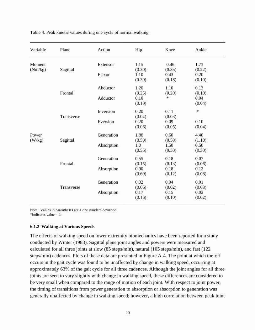
When the power data are examined, some different trends exist as compared to the moment datawhen one considers kinetic measures about the three orthogonal axes during walking.Specifically, the angular velocities are larger in the sagittal plane versus the other two planes,resulting in proportionately larger power values for this primary plane of movement. Forexample, knee and hip peak power generated in the frontal plane is only one-third the respectivesagittal plane values, while the knee and hip peak moments in the frontal plane are larger thantheir respective values in the sagittal plane. Thus, for normal speed walking, it is more importantto conduct a three-dimensional analysis when one is considering joint moments, as compared tojoint powers. In terms of describing the joint power results in Appendix A, in the sagittal plane,the largest peak power generated is at the ankle (just before toe-off), while the largest peakpower absorbed is at the knee. Both of these occur in the sagittal plane. The peak powerabsorbed at the hip in the frontal and sagittal planes is approximately equal. Similar to the jointmoment results, the joint powers for the ankle in the frontal plane and for all three joints in thetransverse plane were quite small. During normal walking, toe-off occurs at approximately 60%of the gait cycle, and it is evident from these figures that the moments and powers are generallysmall during the swing phase (60% to 100% gait cycle). An exception to this is the powerabsorbed at the knee (see Figure A-2) in the sagittal plane since the hamstring muscles provide abraking action to knee extension before heel contact. A summary of the peak kinetic valuesassociated with all three planes of motion for each joint is given in Table 4.

20

Table 4. Peak kinetic values during one cycle of normal walking

______________________________________________________________________________

Variable Plane Action Hip Knee Ankle______________________________________________________________________________

Moment Extensor 1.15 0.46 1.73(Nm/kg) Sagittal (0.30) (0.35) (0.22)

Flexor 1.10 0.43 0.20(0.30) (0.18) (0.10)

Abductor 1.20 1.10 0.13Frontal (0.25) (0.20) (0.10)

Adductor 0.10 * 0.04(0.10) (0.04)

Inversion 0.20 0.11 *Transverse (0.04) (0.03)

Eversion 0.20 0.09 0.10(0.06) (0.05) (0.04)

Power Generation 1.80 0.60 4.40(W/kg) Sagittal (0.50) (0.50) (1.10)

Absorption 1.0 1.50 0.50(0.55) (0.50) (0.30)

Generation 0.55 0.18 0.07Frontal (0.15) (0.13) (0.06)

Absorption 0.90 0.18 0.12(0.60) (0.12) (0.08)

Generation 0.02 0.04 0.01Transverse (0.06) (0.02) (0.03)

Absorption 0.17 0.15 0.02(0.16) (0.10) (0.02)

______________________________________________________________________________Note: Values in parentheses are ± one standard deviation.*Indicates value ≈ 0.

6.1.2 Walking at Various Speeds

The effects of walking speed on lower extremity biomechanics have been reported for a studyconducted by Winter (1983). Sagittal plane joint angles and powers were measured andcalculated for all three joints at slow (85 steps/min), natural (105 steps/min), and fast (122steps/min) cadences. Plots of these data are presented in Figure A-4. The point at which toe-offoccurs in the gait cycle was found to be unaffected by change in walking speed, occurring atapproximately 63% of the gait cycle for all three cadences. Although the joint angles for all threejoints are seen to vary slightly with change in walking speed, these differences are considered tobe very small when compared to the range of motion of each joint. With respect to joint power,the timing of transitions from power generation to absorption or absorption to generation wasgenerally unaffected by change in walking speed; however, a high correlation between peak joint

21

powers and walking velocity was observed for all three joints. Several power bursts have beenidentified at the hip, knee, and ankle joints during one cycle of normal walking (see Figure A-4).Peak values occurring during these power bursts are presented in Table 5. An increase in peakjoint power was shown to occur with increased walking speed for all power bursts except H1.

Table 5. Peak power values during one cycle of walking at three different cadences

______________________________________________________________________________

Cadence Hip Knee Ankle(steps/min) H1* H2 H3 K1 K2 K3 K4 A1 A2______________________________________________________________________________

85 0.16 -0.15 0.33 -0.35 0.10 -0.60 -0.51 -0.48 2.08

105 0.31 -0.25 0.68 -0.60 0.35 -0.70 -0.85 -0.50 3.33

122 0.26 -0.90 1.39 -2.10 1.08 -1.65 -1.30 -0.60 5.00______________________________________________________________________________Note: Powers given in watts per kilogram body mass. Positive values indicate power generated; negative values indicate powerabsorbed.*The locations of each power burst within the gait cycle are indicated in Figure A-4.

6.1.3 Walking With Loads

In 2000, Harman, Hoon, Frykman, and Pandorf reported about the effects of load carriage onlower extremity biomechanics during walking. Joint angle data were collected and joint momentswere calculated for carried backpack loads of 6, 20, 33, and 47 kg while subjects walked at aspeed of approximately 1.33 m/s; plots of these data are given in Figure A-5. In contrast tochange in walking speed, the instant when toe-off occurs in the gait cycle was affected by changein carried load. As carried load increased from 6 to 47 kg, the duration of the stance phase wasobserved to increase from approximately 63.4% to 65.2% of the gait cycle. Timing of transitionsfrom flexion to extension and extension to flexion also appears to be affected by change incarried load. The effect of change in carried load on hip joint angles was not reported, but slightchanges in knee and ankle joint angles were. Peak knee flexion during mid-stance (≈ 10% to

30% gait cycle) was found to increase from approximately 22.5 to 27.5 degrees, while peak kneeflexion at the transition from initial to mid-swing (≈ 72% gait cycle) was found to decrease from

approximately 68 to 64 degrees with an increase in carried load. At the ankle, peak dorsiflexionduring terminal stance (≈ 30% to 50% gait cycle) was found to decrease from approximately11.5 to 10 degrees, and peak plantarflexion at the transition from mid- to terminal swing (≈ 90%

gait cycle) was found to decrease from approximately 5 to 3.5 degrees with an increase in carriedload. As with the joint angles, timing of transitions from extensor to flexor and flexor to extensormoments, as well as peak values obtained at each joint, appears to be affected by change incarried load. At the hip, peak extensor moment values during loading response, as well as peakflexor moment values during terminal stance, were found to increase with an increase in carried

22

load. Peak knee extensor moment values during mid-stance and peak ankle plantarflexor momentvalues during terminal stance were also found to increase with an increase in carried load, whilepeak knee flexor and ankle dorsiflexor moments did not follow a monotonically increasing trend.The peak extensor and flexor moment values obtained at each joint under each of the fourdifferent backpack loads are summarized in Table 6.

Table 6. Peak moment values during one cycle of walking with four different backpack loads

______________________________________________________________________________

Load Hip Knee Ankle(kg) Extensor Flexor Extensor Flexor Plantarflexor Dorsiflexor______________________________________________________________________________

6 0.81 0.78 0.72 0.34 1.76 0.13

20 0.85 0.88 0.81 0.40 2.08 0.10

33 0.88 1.12 1.20 0.33 2.15 0.20

47 1.00 1.24 1.37 0.35 2.41 0.16______________________________________________________________________________Note: Moments given in newton meters per kilogram body mass.

As previously mentioned, the mass, size, and inertial properties of the exoskeleton are assumedto be equivalent to those of a human. Because humans vary in these dimensions, exoskeletonsmust be designed to fit a range of soldiers. Typically, equipment is developed to fit soldiers fromthe 5th to 95th percentile for a particular body dimension. For the analyses in this report, bodymass is the dimension that will be used because of the assumption that joint moments and jointpowers scale linearly with mass. Also, the body masses of male soldiers will be used becauseaccording to the DARPA BAA, the exoskeleton is initially being developed for combat soldiers.

According to the anthropometric survey of U.S. Army personnel conducted in 1988 (Gordon etal., 1989), the body masses of 5th and 95th percentile male soldiers are 61.59 and 98.07 kg,respectively. For normal walking, we obtain estimates of the range of peak sagittal plane kineticvalues for male soldiers from the 5th to 95th percentile (by mass) by multiplying the given bodymass by the moment and power values given in Table 4. The resulting ranges of peak momentand power values obtained by these calculations are presented in Table 7.

23

Table 7. Range of peak kinetic values for 5th to 95th percentile male soldiers during one cycle of normalwalking

______________________________________________________________________________

Variable Action Hip Knee Ankle______________________________________________________________________________

Moment(Nm) Extensor 71 to 113 28 to 45 106 to 169

Flexor 68 to 108 26 to 42 12 to 20

Power(W) Generation 111 to 177 37 to 59 271 to 432

Absorption 62 to 98 92 to 147 31 to 49______________________________________________________________________________

6.2 Running

Sagittal plane kinetic data for the stance phase of “normal” running at a moderate pace ofapproximately 3.8 m/s have been published by DeVita, Torry, Glover, and Speroni (1996); plotsof these data are shown in Figure A-6. Peak moment and power values associated with these dataare summarized in Table 8. When the joint moment data are examined, it can be seen that,similar to walking, the largest peak extensor moment occurs at the ankle (in this case, near mid-stance, ≈ 50% stance phase), while the largest peak flexor moment again occurs at the hip. With

respect to joint power, the largest peak power generation again occurs at the ankle, and thelargest peak power absorption value is found at the knee during the loading response (≈ 10% to

30% stance phase). With the exceptions of peak hip and ankle flexor moments, all the peakkinetic values for running at a moderate pace are much higher than those for walking at a naturalpace (see Table 4).

Table 8. Peak kinetic values during stance phase of normal running at 3.8 m/s

______________________________________________________________________________

Variable Action Hip Knee Ankle______________________________________________________________________________

Moment(Nm/kg) Extensor 2.81 (0.30) 2.74 (0.38) 3.34 (0.12)

Flexor 0.61 (0.23) 0.53 (0.00) *

Power (W/kg) Generation 3.80 (1.52) 12.9 (2.08) 17.5 (0.76)

Absorption 11.0 (4.18) 18.2 (1.52) 12.2 (0.69)______________________________________________________________________________Note: Values in parentheses are ± one standard deviation.* indicates a value ≈ 0.

24

Arampatzis, Brüggemann, and Metzler (1999) have reported about the effects of change in speedon lower limb biomechanics during the stance phase of running. Sagittal plane data werecollected at the knee and ankle for subjects running at five speeds ranging from jogging(2.61 m/s) to sprinting (6.59 m/s), and the resulting joint moments and powers occurring duringthe stance phase were calculated. Plots of these results are shown in Figure A-7, and a summaryof the peak moment and power values obtained is provided in Table 9. Similar to the effects ofchange in speed on walking biomechanics, all the peak kinetic values during the stance phase ofrunning are shown to increase with increased speed.

As with walking, an estimate of the peak kinetic values for the range of 5th to 95th percentilemale soldiers running at a moderate pace can be obtained. This is done by multiplying thecorresponding body masses with the mean normalized joint moment and power data for running,as reported in Table 8. The resulting values are presented in Table 10.

Table 9. Peak kinetic values during the stance phase of running at five different speeds

______________________________________________________________________________

Knee AnkleSpeed Moment Power Moment Power (m/s) Extensor Generated Absorbed Extensor Generated Absorbed______________________________________________________________________________

2.61 2.00 4.23 7.75 2.45 6.60 3.303.55 2.57 5.62 12.0 2.78 10.1 4.604.47 2.64 6.92 13.2 2.99 12.3 5.905.60 2.74 9.89 14.2 3.20 16.4 8.706.59 2.99 10.7 16.8 3.44 21.0 12.2______________________________________________________________________________Note: Moments given in newton meters per kilogram; powers given in watts per kilogram.

Table 10. Peak moment values for 5th to 95th percentile male soldiers during one cycle of running at amoderate pace (3.8 m/s)

______________________________________________________________________________

Variable Action Hip Knee Ankle______________________________________________________________________________

Moment(Nm) Extensor 173 to 276 168 to 268 206 to 328

Flexor 37 to 60 33 to 52 *

Power(W) Generation 234 to 373 796 to 1267 1076 to 1714

Absorption 679 to 1081 1123 to 1789 749 to 1192______________________________________________________________________________Note: * indicates a value ≈ 0.

25

6.3 Stair Climbing

In 1980, Andriacchi, Anderson, Fermier, Stern, and Galante performed an analysis of stair ascentand descent, reporting the stance phase joint moments for all three planes of motion. In this study,subjects ascended and descended a three-step staircase, and kinematic data were collected for onestride between the first and third steps. Joint moments were calculated during the stance phase forall three planes of motion at each joint, and these resulting data are shown in Figure A-8. Asummary of the peak joint moment values obtained for each plane of motion is presented inTable 11. During the stance phase of stair ascent, the largest joint moments appear to haveoccurred in the sagittal plane, but peak abductor moments in the frontal plane are also significant,with values equal to approximately one-half to three-quarters of their corresponding peak extensormoments. Similarly, during the stance phase of stair descent, the largest peak joint moments againappear to have occurred in the sagittal plane, while peak abductor moments range in value fromapproximately one-half to two-thirds of their corresponding peak extensor moment. Transversemoments during the stance phase of both stair ascent and descent appear to be rather small for allthree joints.

Table 11. Three-dimensional peak moment values during the stance phase of normal stair ascent anddescent

______________________________________________________________________________

Plane Action Hip Knee Ankle______________________________________________________________________________

Ascent Sagittal Extensor 1.27 0.89 1.34Flexor * 0.28 *

Frontal Abductor 0.63 0.77 0.60Adductor 0.05 * *

Transverse Inversion 0.03 0.08 0.02Eversion 0.21 0.05 0.10

Descent Sagittal Extensor 0.99 1.55 1.20Flexor 0.35 0.70 *

Frontal Abductor 0.65 0.44 0.63Adductor 0.14 0.14 *

Transverse Inversion 0.04 0.13 0.03Eversion 0.21 0.03 0.06

______________________________________________________________________________Note: Moments given in newton meters per kilogram* indicates a value ≈ 0.

Sagittal plane lower extremity joint powers have been published by Duncan, Kowalk, andVaughan (1997) for normal stair ascent and descent. In their study, subjects also ascended anddescended a three-step staircase, kinematic data were collected for each lower extremity joint,and joint powers were calculated with a six-degree-of-freedom approach. Plots of the resultingjoint powers are shown in Figure A-9, and a summary of the peak power values obtained for

26

each joint is given in Table 12. During both stair ascent and descent, the largest peak powergeneration appears to have occurred at the ankle, while the largest peak power absorption duringstair ascent occurred at the knee and during stair descent at the ankle. In contrast to walking,during stair ascent, peak power generation at the knee is approximately four times greater, whilepeak power generation at the ankle decreases by about one-third. Peak power absorption valuesat all three joints are also reduced by one-half to three-fourths in comparison to those values seenduring walking. The most notable difference between normal walking and stair ascent is the rolereversal of the knee joint from power absorber to power generator. During stair descent, peakpower generation values at all three joints and peak power absorption at the hip are also reducedto approximately one-third to one-half of their corresponding values for normal walking, whilepeak power absorption values at the knee and ankle are approximately one and one-third and fivetimes larger, respectively. The role of the ankle joint is split nearly evenly between powergeneration and absorption, rather than acting solely as a power generator as seen in normalwalking.

Table 12. Peak power values during one cycle of normal stair ascent and descent

______________________________________________________________________________

Action Hip Knee Ankle______________________________________________________________________________

Ascent Generation 1.50 2.10 2.90Absorption 0.50 0.70 0.10

Descent Generation 0.65 0.25 2.05Absorption 0.50 2.00 2.40

______________________________________________________________________________Note: Powers given in watts per kilogram.

Sagittal plane peak kinetic values during stair ascent and descent for the range of 5th to 95thpercentile male soldiers can again be estimated through multiplication of the appropriate bodymasses with the normalized sagittal plane joint moment data reported in Table 11 and thenormalized joint power data reported in Table 12. The resulting values are presented in Table 13.

27

Table 13. Peak kinetic values for 5th to 95th percentile male soldiers during one cycle of stair ascent anddescent

______________________________________________________________________________

Variable Action Hip Knee Ankle______________________________________________________________________________

Ascent Moment Extensor 78 to 125 55 to 87 83 to 131 (Nm) Flexor * 17 to 27 *Power Generation 92 to 147 129 to 206 179 to 284(W) Absorption 31 to 49 43 to 69 6 to 10

Descent Moment Extensor 61 to 97 95 to 152 74 to 118(Nm) Flexor 22 to 34 43 to 69 *Power Generation 40 to 64 15 to 25 123 to 195(W) Absorption 31 to 49 123 to 196 148 to 235

______________________________________________________________________________Note: * indicates a value ≈ 0.

6.4 Jumping

The lower extremity kinetics of a running vertical jump with a single-legged take-off have beenreported by Stefanyshyn and Nigg (1998). In this study, five subjects performed running verticaljumps, and kinematic data were collected for the stance phase of the take-off leg before toe-off.Plots of the averaged data from this report are shown in Figure A-10, where the normalizedstance phase represents time periods ranging from 0.23 to 0.35 seconds, 0% stance phase is theinstant of foot contact with the floor, and 100% stance phase is the instant of toe-off. The peakkinetic values obtained for each joint during the running vertical jump are summarized inTable 14. During the running vertical jump, it appears that the largest peak extensor momentoccurs at the hip, while the largest peak flexor moment occurs at the knee. With respect to jointpower, the largest peak generation during the running vertical jump occurs at the ankle, and thelargest peak power absorption appears to occur at the ankle.

Table 14. Peak kinetic values during the stance phase before toe-off of a running vertical jump

______________________________________________________________________________

Variable Action Hip Knee Ankle______________________________________________________________________________

Moment Extensor 4.18 (1.15) 2.77 (0.72) 4.08 (0.59)(Nm/kg) Flexor 0.35 (1.47) 1.07 (0.45) 0.09 (0.29)

Power Generation 9.24 (6.48) 10.7 (8.15) 26.8 (3.33)(W/kg) Absorption 3.02 (0.56) 6.09 (5.31) 7.81 (3.74)______________________________________________________________________________Note: Values in parentheses are ± one standard deviation.

28

We estimated the range of peak kinetic values for 5th to 95th percentile male soldiers during thetake-off stance phase of a running vertical jump by multiplying their respective body masses bythe values given in Table 14. The values resulting from this process are presented in Table 15.

Table 15. Peak kinetic values for 5th to 95th percentile male soldiers during the stance phase before toe-off of a running vertical jump

______________________________________________________________________________

Variable Action Hip Knee Ankle______________________________________________________________________________

Moment Extensor 257 to 410 171 to 272 251 to 400(Nm) Flexor 22 to 35 66 to 106 5 to 9

Power Generation 569 to 906 658 to 1048 1648 to 2624(W) Absorption 186 to 297 375 to 598 481 to 766______________________________________________________________________________

6.5 Kneeling

Very little published biomechanics data exist for kneeling, but some information concerningrange of motion and joint moments is presented in an American Society of Biomechanics (ASB)conference abstract (Nagura et al., 2000) and American Society of Mechanical Engineers(ASME) conference abstract (Nagura, Dyrby, Alexander, and Andriacchi, 2001). The ASBabstract discusses results for all three joints from a study in which subjects performed four tasks,single- and double-legged rises from a kneeling position, and single- and double-legged kneelingfrom a standing position. Ranges of motion for each joint (approximately 65.9 degrees at the hip,149.7 degrees at the knee, and 88.6 degrees at the ankle) were similar across the four differenttasks. These values are significantly higher than those seen during normal walking or stairclimbing. During the single-legged rise, the largest peak extensor moment occurred at the hip(≈ 1.4 Nm/kg), followed closely by the knee (≈ 1.3 Nm/kg), and ankle (≈ 0.8 Nm/kg). Peak

flexor moments were negligible for all three joints during this task. During the double-leggedrise, the largest peak extensor moment occurred at the knee (≈ 2.4 Nm/kg), followed by the ankle(≈ 1.4 Nm/kg), and hip (≈ 0.2 Nm/kg). Peak flexor moments were again negligible at the knee

and ankle, but the peak hip flexor moment was approximately 1.4 Nm/kg. Joint moments for thesingle- and double-legged kneeling tasks were reported to be similar to those for the single- anddouble-legged rising tasks. In the ASME abstract, range of motion and joint moments at the kneeduring the same four tasks are discussed. Range of motion at the knee is reported to vary fromapproximately 126 to 152 degrees, depending on the task. Peak knee extensor moments for thesingle-legged rising and kneeling tasks are reported to be approximately 1.0 and 1.1 Nm/kg,respectively, while peak knee extensor moments for the double-legged rising and kneeling tasksare reported to be approximately 2.3 and 2.1 Nm/kg, respectively.

29

7. Lower Limb Peak Power Profiles for Soldier Missions

7.1 Procedure

With the hip, knee, and ankle joint power data reported in biomechanical literature and a seriesof simple steps, lower extremity peak power profiles were generated for two soldier missionsconsisting of various tasks. Several assumptions were made in this process. Each of these fiveassumptions should be considered as potential sources of error in the values resulting from thisprocess.

1. Increasing carried load has the same effect on peak joint power as does increasingbody mass,

2. The power values observed in the frontal plane are generally small and in thetransverse plane generally very small in comparison to those in the sagittal plane; therefore, onlythe power generated and absorbed in the sagittal plane was considered,

3. Normal gait is symmetric,

4. Based on range of motion and peak extensor moments, peak power values forassuming and getting out of kneeling and prone positions, crawling, and climbing a ladder can beapproximated with values of stair ascent, and

5. Power values of other lower extremity joints, such as the metatarsophalangeal joint,are small and therefore not included in the calculation of peak power.

The first step in this process involved the development of mission spreadsheets containing time,task, and load information for each of the missions examined (see Appendix B, Table B-1).Estimations of the peak and average powers required for each of the task and load combinationswere then made according to the method described in the following paragraph. Finally, the peakpower values obtained for each task and load combination were entered into the missionspreadsheets appropriately, and peak power profiles were generated for each mission scenario.This process could be applied to any mission scenario that anyone would want to create.

Several steps were taken in order to estimate the peak and average powers required for each taskand load combination. Based on the first assumption listed previously, we estimated the totalpower required during one cycle of each task and load combination by first multiplying theappropriate normalized hip, knee, and ankle joint power data for each task by the correct massvalue. The mass values used in this calculation are as follow: 50th percentile male soldier(≈ 77 kg) plus fighting load (≈ 24 kg) or sustainment load (≈ 35 kg), resulting in values of

101 and 112 kg, respectively. The mass of the 50th percentile male soldier is used to keep theanalyses simple and to provide initial guidance. Table 16 shows the individual masses of eachcomponent included in the fighting and sustainment loads. Then, based on the second and thirdassumptions listed previously, the absolute joint power data for each task and load combination

30

(except for the running vertical jump) were plotted simultaneously for the hip, knee, and anklejoints of the left and right lower limbs, offsetting the curves of each leg by 50% of the gait cycle(see Figure B-1a). For the running vertical jump, the absolute joint power data were simultan-eously plotted for the hip, knee, and ankle joints of the take-off leg only. The actuators of theexoskeleton will need to develop power during the power generation and power absorptionphases of these tasks; therefore, the absolute values of the resulting joint powers for each taskand load combination were taken. Next, a total power curve was obtained for each task and loadcombination via the equation

∑=N

ii tPtTP )()( ,

in which t is percent time in the gait cycle (i.e., between 0% and 100%), TP is the total power, Pis the joint power, i indicates the joint (i.e., left or right hip, knee, or ankle), and N is the numberof joints (three for running vertical jump; six for all other tasks). Finally, the peak power valuewas obtained through identification of the maximum value along the total power curve (seeFigure B-1b), and the average power value was calculated for each task and load combination.These values are summarized in Table 17.

Table 16. Loads carried______________________________________________________________________________

Load Mass (kilograms)

Fighting Load Battle dress uniform 1.7 Boots 1.5 Personal armored system for ground troops (PASGT) helmet 1.4 PASGT vest 5.4 M16A2 3.7 Bayonet 0.6 Load-carrying equipment (LCE) 0.7 Ammunition pouches (2) with 180 rounds in six magazines 3.2 Hand grenades (2) 0.9 Canteens (2) with water 2.9 Protective mask and hood 1.3 Poncho 0.7TOTAL 24.0Existence Load Army lightweight individual carrying equipment (ALICE) pack 1.1 Additional clothing 0.5 Personal hygiene kit 1.2 Food 1.3 Sleeping bag 3.4 Sleeping mat 1.6Field Jacket and Gloves 1.9TOTAL 11.0Sustainment Load Fighting load + existence load 35.0

31

Table 17. Peak and average power values for typical soldier tasks______________________________________________________________________________

Total Mass (soldier plus carried load) Task Fighting (101 kg) Sustainment (112 kg)______________________________________________________________________________

Slow Walk (85 steps/min) 283 (119) 314 (131)

Natural Walk (105 steps/min) 411 (180) 456 (200)

Fast Walk (122 steps/min) 693 (315) 769 (349)

Jog (2.7 m/s) 1966 (1041) 2180 (1155)

Run (3.8 m/s) 3147 (1693) 3489 (1877)

Sprint (7.6 m/s) 5547 (3522) 6151 (3906)

Running Vertical Jump 3559 (1325) 3947 (1369)

Ascend Stairs 501 (229) 556 (254)

Descend Stairs 478 (270) 530 (300)______________________________________________________________________________Note: All peak(average) power values are given in watts. All values represent absolute power for all six lower extremity joints(left and right hip, knee, and ankle joints) during the given task and load combination, except for jumping, which assumes arunning jump with single-legged take-off.

7.2 Mission Scenarios

7.2.1 Movement to Contact

In the movement-to-contact mission, a platoon is moving through a rural area. They are carryingtheir sustainment loads (35 kg). At the beginning of the mission, the platoon marches and takesrest breaks according to Field Manual (FM) 21-18 (Department of the Army, 1990). When theplatoon makes contact with the enemy, they drop their existence loads and carry only theirfighting loads (24 kg). The platoon members who will engage the enemy use cover and conceal-ment to move according to FM 7-8 (Department of the Army, 1992) and FM 21-75 (Departmentof the Army, 1984). This movement includes a series of rushes, that is, running for 3 to 5 seconds,going prone, crawling, rolling left or right, getting up and repeating the sequence until they arewithin approximately 100 yards of the enemy. They engage the enemy from covered positionsand then move in another series of rushes to close with and destroy the enemy. They consolidateand reorganize. Then they remove casualties. After resting briefly, they return to pick up theirexistence loads. They repeat the tasks from the first part of the mission and engage another groupof enemy soldiers. After they go back to pick up their existence loads this time, they march andtake rest breaks until they find a safe place to rest for the night. The entire mission takes 16 hours,and the resulting peak power profile is shown in Figure B-2 for a 50th percentile male soldier.With the assumptions stated earlier concerning the exoskeleton’s design, its power requirementscan be estimated from Figure B-2 and assumed to be within 20% of their actual values. Thus, apower supply that is capable of producing a nearly constant mean value of approximately 200

32

±40 W, and peak values of 500 ±100 to 5500 ±1100 W at frequencies ranging from

approximately 2 to 4 Hz, depending on the task, would be required for this mission.

7.2.2 Clear Building

In this scenario, a platoon is going to clear a building during daylight. The soldiers are carryingtheir fighting loads (24 kg). The building is three stories high and has a basement. Each floor isapproximately 17,850 square feet. There are six to ten enemy soldiers in the building. The platoonfollows FM 90-10-1 (Department of the Army, 1993) and FM 7-8 (Department of the Army,1992). The platoon divides into squads. One squad provides security outside the building. Anoth-er squad is held in reserve. Two squads enter and clear the building. The two squads that enterand clear the building approach from the back. They use a ladder and enter a second floor roomthrough a window. Then they work their way to the stairs. Inside the building, one squad isresponsible for securing the stairs, and the other squad is responsible for clearing the rooms. Thesquad that clears the rooms divides into two fire teams and goes up to the third floor. One fireteam provides security in the hallway while the other team clears rooms. A fire team clears aboutfour to six rooms and then switches to security while the other team clears rooms. They alternateroles in this fashion, clearing the third floor, the second floor, the first floor, and finally, the base-ment. The entire mission takes 2 hours and 12.5 minutes, and the resulting peak power profile isshown in Figure B-3 for a 50th percentile male soldier on one of the room-clearing fire teams. Aswith the movement-to-contact mission, the exoskeleton’s power requirements during a clear-building mission can be estimated from Figure B-3 and assumed to be within 20% of their actualvalues. Although this power profile varies much more than that of the previous scenario, itappears that a power supply capable of producing a mean power value between 100 ±20 and 300±60 W, and peak values of 400 ±80 to 3500 ±700 W at 2 to 4 Hz, depending upon the task, would

be required for such a mission.

8. Conclusions

The goals for this work were to determine the angles, torques, and powers at the lower limb jointsof an exoskeleton and to estimate the requirements for a system to power the lower limbs of thatexoskeleton. It was assumed that the angles, torques, and powers could be estimated from bio-mechanical data collected from humans. Based on biomechanical data gathered from various pub-lished sources, we have provided estimates of angle, torque, and power values at the hip, knee, andankle joints during various activities. Estimated peak power values were also determined for twohypothetical missions to produce lower limb peak power profiles. Keeping in mind the limitationsand variability of kinematic and kinetic data and the assumptions made in the application of suchdata to an exoskeleton, these estimated values (see Appendix A, Table 17, and Figures B-2 andB-3) could be used to design lower limb joints and actuators and to size the power supply for anexoskeleton.

33

References

Andriacchi, T.P., Anderson, G.B.J., Fermier, R.W., Stern, D., & Galante, J.O. (1980). A study oflower limb mechanics during stair climbing. Journal of Bone Joint Surgery, 62-A(5), 749-757.

Arampatzis, A., Brüggemann, G.P., & Metzler, V. (1999). The effect of speed on leg stiffnessand joint kinetics in human running. Journal of Biomechanics, 32, 1349-1353.

Challis, J.H., & Kerwin, D.G. (1996). Quantification of the uncertainties in resultant jointmoments computed in a dynamic activity. Journal of Sports Sciences, 14, 219-231.

Clauser, C.E., McConville, J.T., & Young, J.M. (1969). Weight, volume, and center of mass ofsegments of the human body. (Technical Report AMRL TR 69-70). Wright-Patterson AirForce Base, OH: Aerospace Medical Research Laboratory.

Defense Advanced Research Projects Agency (2000). Exoskeletons for Human PerformanceAugmentation (EHPA). (Commerce Business Daily, Broad Agency Announcement No. 00-34). Washington, DC: Department of Commerce.

Department of the Army (1984). FM (Field Manual) 21-75: Combat Skills of the Soldier.Washington, DC: Headquarters, Department of the Army.

Department of the Army (1990). FM (Field Manual) 21-18: Foot Marches. Washington, DC:Headquarters, Department of the Army.

Department of the Army (1992). FM (Field Manual) 7-8: Infantry Rifle Platoon and Squad.Washington, DC: Headquarters, Department of the Army.

Department of the Army (1993). FM (Field Manual) 90-10-1: An Infantryman’s Guide toCombat in Built-Up Areas. Washington, DC: Headquarters, Department of the Army.

DeVita, P., Torry, M., Glover, K.L., & Speroni, D.L. (1996). A functional knee brace alters jointtorque and power patterns during walking and running. Journal of Biomechanics, 29(5), 583-588.

Duncan, J.A., Kowalk, D.L., & Vaughan, C.L. (1997). Six degree of freedom joint power in stairclimbing. Gait & Posture, 5, 204-210.

Edman, K.A.P., Elzinga, G., & Noble, H.I.M. (1978). Enhancement of mechanical performanceby stretch during tetanic contractions of vertebrate skeletal muscle fibers. Journal ofPhysiology, London, 281, 139-155.

34

Eng, J.J., & Winter, D.A. (1995). Kinetic analysis of the lower limbs during walking: Whatinformation can be gained from a three-dimensional model? Journal of Biomechanics, 28(6),753-758.

Fukunaga, T., Matsuo, A., Yuasa, K., Fujimatsu, H., & Asahina, K. (1980). Effect of runningvelocity on external mechanical power output. Ergonomics, 23(2), 123-136.

Glitsch, U., & Baumann, W. (1997). The three-dimensional determination of internal loads in thelower extremity. Journal of Biomechanics, 30(11/12), 1123-1131.

Gordon, A.M., Huxley, A.F., & Julian, F.J. (1966). The variation in isometric tension withsarcomere length in vertebrate muscle fibers. Journal of Physiology, 184, 170-192.

Gordon, C.C., Churchill, T., Clauser, C.E., Bradtmiller, B., McConville, J.T., Tebbetts, I., &Walker, R.A. (1989). 1988 anthropometric survey of U.S. Army personnel: Summarystatistics report 1989 (Technical Report Natick/TR-89-027). Natick, MA: U.S. Army NatickResearch, Development, and Engineering Center.

Harman, E., Hoon, H.K., Frykman, P., & Pandorf, C. (2000). The effects of backpack weight onthe biomechanics of load carriage (Technical Report USARIEM TR-00/17). Natick, MA:U.S. Army Research Institute of Environmental Medicine.

Hill, A.V. (1938). The heat of shortening and the dynamic constants of muscle. ProceedingsRoyal Society London, Ser. B, 126, 136-195.

Inman, V.T., Ralston, H.J., Todd, F., & Lieberman, J.C. (1981). In J. Rose and J. Gamble (Eds.),Human walking, page 26. Baltimore, MD: Williams & Wilkins.

Jacobs, R., Bobbert, M.F., & van Ingen Schenau, G.J. (1996). Mechanical output from individualmuscles during explosive leg extensions: the role of biarticular muscles. Journal ofBiomechanics, 29(4), 513-523.

Kadaba, M.P., Ramakrishnan, H.K., & Wootten, M.E. (1990). Measurement of lower extremitykinematics during level walking. Journal of Orthopedic Research, 8(3), 383-392.

Lloyd R., & Cooke C.B. (2000). Kinetic changes associated with load carriage using tworucksack designs. Ergonomics, 43(9), 1331-1341.

Martin, P.E. (1985). Mechanical and physiological responses to lower extremity loading duringrunning. Medicine and Science in Sports and Exercise, 17, 427-433.

Martin, P.E., & Marsh, A.P. (1992). Step length and frequency effects on ground reaction forcesduring walking. Journal of Biomechanics, 25(10), 1237-1239.

McCaw, S.T., & DeVita, P. (1995). Errors in alignment of center of pressure and footcoordinates affect predicted lower extremity torques. Journal of Biomechanics, 28(8), 985-988.

35

McClay, I., & Manal, K. (1999). Three-dimensional kinetic analysis of running; significance ofsecondary planes of motion. Medicine and Science in Sports and Exercise, 31(11), 1629-1637.

McMahon, T.A., Valiant, G., & Frederick, E.C. (1987). Groucho Running. Journal of AppliedPhysiology, 62(6), 2326-2337.

Minetti, A.E., Ardiago, L.P., & Saibele, F. (1994). The transition between walking and runningin humans: metabolic and mechanical aspects at different gradients. Acta PhysiologicaScandinavica, 150, 315-323.

Nagano, A., Gerritsen, K.G.M., & Fukashiro, S. (2000). A sensitivity analysis of the calculationof mechanical output through inverse dynamics: a computer simulation study. Journal ofBiomechanics, 33(10), 1313-1318.

Nagura, T., Dyrby, C.O., Alexander, E.J., & Andriacchi, T.P. (2001). Mechanical loads on theknee joint during deep flexion. ASME Bioengineering Conference. BDE, 50, 393-395.

Nagura, T., Dyrby, C., Chaudhari, A., MacMahon, J., Alexander, E., & Andriacchi, T. (2000).Evaluation of dynamic joint loading during rising and descending to a kneeling position.ASB Annual Conference. http://asb-biomech.org/abstracts2000/pdf/090.pdf.

Obusek, J.P., Harman, E.A., Frykman, P.N., Palmer, C.J., & Bills, R.K. (1997). The relationshipof backpack center of mass location to the metabolic cost of load carriage. Medicine andScience in Sports and Exercise, 29(5), S205.

Sadeghi, H., Allard, P., Prince F., & Labelle, H. (2000). Symmetry and limb dominance in able-bodied gait: a review. Gait and Posture, 12, 34-45.

Smidt, G.L. (1973). Biomechanical analysis of knee flexion and extension. Journal ofBiomechanics, 69, 79-92.

Soule, R.G., & Goldman, R.F. (1969). Energy cost of loads carried on the head, hands or foot.Journal of Applied Physiology, 27, 687-690.

Stefanyshyn, D.J., & Nigg, B.M. (2000). Influence of midsole bending stiffness on joint energyand jump height performance. Medicine and Science in Sports and Exercise, 32(2), 471-476.

Stefanyshyn, D.J., & Nigg, B.M. (1998). Contribution of the lower extremity joints tomechanical energy in running vertical jumps and running long jumps. Journal of SportsSciences, 16, 177-186.

Tilbury-Davis, D.C., & Hooper R.H. (1999). The kinetic and kinematic effects of increasing loadcarriage upon the lower limb. Human Movement Science, 18, 693-700.

36

Van Soest, A.J., Schwab, A.L., Bobbert, M.F., & van Ingen Schenau, G.J. (1993). The influenceof the biarticularity of the gastrocnemius muscle on vertical-jumping achievement. Journal ofBiomechanics, 26(1), 1-8.

Winter, D.A. (1983). Biomechanical motor patterns in normal walking. Journal of MotorBehavior, 15(4), 302-330.

Winter, D.A. (1984). Kinematic and kinetic patterns in human gait: Variability and compensatingeffects. Human Movement Science, 3, 51-76.

Figure A-1. Hip joint angles, moments, and powers in the sagittal, frontal, and transverse planes during one cycle of normal walking. (Solid linesare mean values and dotted lines are ± one standard deviation.)

Sagittal Plane Frontal Plane Transverse Plane

Percent Gait Cycle Percent Gait Cycle Percent Gait Cycle

Ang

le (

degr

ees)

M

omen

t (N

m/k

g)

Pow

er (

W/k

g)

Fle

xion

Abd

ucti

on

Add

ucti

on

Int.

Rot

atio

n

Ext

. Rot

atio

n

F

lexo

r

Ext

enso

r

Abd

ucto

r

E

xt. R

otat

or

In

t. R

otat

or

Abs

orbe

d

Gen

erat

ed

Abs

orbe

d

Gen

erat

ed

Abs

orbe

d

-10

-8

-6

-4

-2

0

2

4

6

8

10

0 10 20 30 40 50 60 70 80 90 100

-0.4

-0.35

-0.3

-0.25

-0.2

-0.15

-0.1

-0.05

0

0.05

0.1

0 10 20 30 40 50 60 70 80 90 100

-0.3

-0.2

-0.1

0

0.1

0.2

0.3

0 10 20 30 40 50 60 70 80 90 100

-2

-1.5

-1

-0.5

0

0.5

1

0 10 20 30 40 50 60 70 80 90 100

-0.4

-0.2

0

0.2

0.4

0.6

0.8

1

1.2

1.4

1.6

0 10 20 30 40 50 60 70 80 90 100

-2

-1.5

-1

-0.5

0

0.5

1

1.5

2

2.5

0 10 20 30 40 50 60 70 80 90 100

-2

-1.5

-1

-0.5

0

0.5

1

1.5

2

0 10 20 30 40 50 60 70 80 90 100

-10

0

10

20

30

40

50

0 10 20 30 40 50 60 70 80 90 100

-8

-6

-4

-2

0

2

4

6

8

10

0 10 20 30 40 50 60 70 80 90 100

37

Ap

pen

dix A

: Low

er Lim

b K

inem

atics and

Kin

etics for Variou

s Activities

Figure A-2. Knee Joint angles, moments, and powers in the sagittal, frontal and transverse planes during one cycle of normal walking.

Sagittal Plane Frontal Plane Transverse Plane

Percent Gait Cycle Percent Gait Cycle Percent Gait Cycle

Ang

le (

degr

ees)

M

omen

t (N

m/k

g)

Pow

er (

W/k

g)

F

lexi

on

A

dduc

tion

Int.

Rot

atio

n

Ext

. Rot

atio

n

F

lexo

r

Ext

enso

r

Abd

ucto

r

E

xt. R

otat

or

In

t. R

otat

or

A

bsor

bed

Gen

erat

ed

Abs

orbe

d

Gen

erat

ed

Abs

orbe

d

-8

-6

-4

-2

0

2

4

6

8

10

0 10 20 30 40 50 60 70 80 90 100

-0.3

-0.25

-0.2

-0.15

-0.1

-0.05

0

0.05

0.1

0 10 20 30 40 50 60 70 80 90 100

-0.2

-0.15

-0.1

-0.05

0

0.05

0.1

0.15

0.2

0 10 20 30 40 50 60 70 80 90 100

-0.4

-0.3

-0.2

-0.1

0

0.1

0.2

0.3

0.4

0 10 20 30 40 50 60 70 80 90 100

-0.2

0

0.2

0.4

0.6

0.8

1

1.2

1.4

0 10 20 30 40 50 60 70 80 90 100

-2.5

-2

-1.5

-1

-0.5

0

0.5

1

1.5

0 10 20 30 40 50 60 70 80 90 100

-0.8

-0.6

-0.4

-0.2

0

0.2

0.4

0.6

0.8

1

0 10 20 30 40 50 60 70 80 90 100

-10

0

10

20

30

40

50

60

70

0 10 20 30 40 50 60 70 80 90 100

-4

-2

0

2

4

6

8

10

12

0 10 20 30 40 50 60 70 80 90 100

38

Figure A-3. Ankle joint angles, moments, and powers in the sagittal, frontal and transverse planes during one cycle of normal walking.

Sagittal Plane Frontal Plane Transverse Plane

Percent Gait Cycle Percent Gait Cycle Percent Gait Cycle

Ang

le (

degr

ees)

M

omen

t (N

m/k

g)

Pow

er (

W/k

g)

Pla

ntar

flex

ion

Dor

sifl

exio

n

E

xt. R

otat

ion

Pla

ntar

flex

or

Add

ucto

r

A

bduc

tor

Ext

. Rot

ator

Gen

erat

ed

Abs

orbe

d

G

ener

ated

Abs

orbe

d

Gen

erat

ed

0

5

10

15

20

25

30

0 10 20 30 40 50 60 70 80 90 100

-0.06

-0.05

-0.04

-0.03

-0.02

-0.01

0

0.01

0.02

0.03

0.04

0.05

0 10 20 30 40 50 60 70 80 90 100

-0.16

-0.14

-0.12

-0.1

-0.08

-0.06

-0.04

-0.02

0

0.02

0.04

0 10 20 30 40 50 60 70 80 90 100

-0.25

-0.2

-0.15

-0.1

-0.05

0

0.05

0.1

0.15

0 10 20 30 40 50 60 70 80 90 100

-0.15

-0.1

-0.05

0

0.05

0.1

0.15

0.2

0.25

0 10 20 30 40 50 60 70 80 90 100

-2

-1

0

1

2

3

4

5

6

0 10 20 30 40 50 60 70 80 90 100

-0.5

0

0.5

1

1.5

2

2.5

0 10 20 30 40 50 60 70 80 90 100

-20

-15

-10

-5

0

5

10

15

20

0 10 20 30 40 50 60 70 80 90 100

39

(These data not reported.)

Figure A-4. Sagittal plane joint angles and powers during one cycle of walking at three cadences ( = slow, = natural, = fast).

Joint Angle (degrees) Joint Power (W/kg)

Percent Gait Cycle Percent Gait Cycle

Hip

K

nee

Ank

le

Abs

orbe

d

Gen

erat

ed

Gen

erat

ed

A

bsor

bed

G

ener

ated

Ext

ensi

on

Fle

xion

F

lexi

on

P

lant

arfl

exio

n

D

orsi

flex

ion

-1.5

-1

-0.5

0

0.5

1

1.5

2

0 10 20 30 40 50 60 70 80 90 100

-1

0

1

2

3

4

5

6

0 10 20 30 40 50 60 70 80 90 100

-25

-20

-15

-10

-5

0

5

10

15

0 10 20 30 40 50 60 70 80 90 100

-2.5

-2

-1.5

-1

-0.5

0

0.5

1

1.5

0 10 20 30 40 50 60 70 80 90 100

0

10

20

30

40

50

60

70

80

0 10 20 30 40 50 60 70 80 90 100

-15

-10

-5

0

5

10

15

20

25

0 10 20 30 40 50 60 70 80 90 100

A1

A2

K1

K2

K3 K4

H1

H2

H3

40

Figure A-5. Sagittal Plane Joint Angles and Moments During One Cycle of Walking at 1.33 m/s With Four Different Backpack Loads( = 6 kg, = 20 kg, = 33 kg, = 47 kg).

Joint Angle (degrees) Joint Moment (Nm/kg)

Percent Gait Cycle Percent Gait Cycle

Hip

K

nee

Ank

le

Fle

xion

Pla

ntar

flex

ion

Dor

sifl

exio

n

F

lexo

r

Ext

enso

r

E

xten

sor

Pla

ntar

flex

or

-1.5

-1

-0.5

0

0.5

1

1.5

0 10 20 30 40 50 60 70 80 90 100

-0.5

0

0.5

1

1.5

2

2.5

3

0 10 20 30 40 50 60 70 80 90 100

-20

-15

-10

-5

0

5

10

15

0 10 20 30 40 50 60 70 80 90 100

-0.6

-0.4

-0.2

0

0.2

0.4

0.6

0.8

1

1.2

1.4

1.6

0 10 20 30 40 50 60 70 80 90 100

0

10

20

30

40

50

60

70

80

0 10 20 30 40 50 60 70 80 90 100

41

(These data not reported.)

Figure A-6. Sagittal plane joint moments and powers during the stance phase of running at a moderate pace (3.8 m/s). (Solid lines are mean valuesand dotted lines are ± one standard deviation.)

Joint Moment (Nm/kg) Joint Power (W/kg)

Percent Stance Phase Percent Stance Phase

Hip

K

nee

Ank

le

Fle

xor

E

xten

sor

Ext

enso

r

P

lant

arfl

exor

Abs

orbe

d

G

ener

ated

Abs

orbe

d

G

ener

ated

Abs

orbe

d

G

ener

ated

-20

-15

-10

-5

0

5

10

0 10 20 30 40 50 60 70 80 90 100

-15

-10

-5

0

5

10

15

20

0 10 20 30 40 50 60 70 80 90 100

-0.5

0

0.5

1

1.5

2

2.5

3

3.5

4

0 10 20 30 40 50 60 70 80 90 100

-25

-20

-15

-10

-5

0

5

10

15

20

0 10 20 30 40 50 60 70 80 90 100

-1

-0.5

0

0.5

1

1.5

2

2.5

3

3.5

0 10 20 30 40 50 60 70 80 90 100

-1.5

-1

-0.5

0

0.5

1

1.5

2

2.5

3

3.5

0 10 20 30 40 50 60 70 80 90 100

42

Figure A-7. Sagittal plane joint moments and powers during the stance phase of running at five velocities ( = 2.61 m/s, = 3.55 m/s, = 4.47 m/s, = 5.60 m/s, = 6.59 m/s).

Joint Moment (Nm/kg) Joint Power (W/kg)

Percent Stance Phase Percent Stance Phase

Kne

e

A

nkle

E

xten

sor

P

lant

arfl

exor

Abs

orbe

d

Gen

erat

ed

Abs

orbe

d

Gen

erat

ed

-20

-15

-10

-5

0

5

10

15

0 10 20 30 40 50 60 70 80 90 100

-15

-10

-5

0

5

10

15

20

25

0 10 20 30 40 50 60 70 80 90 100

-0.5

0

0.5

1

1.5

2

2.5

3

3.5

4

0 10 20 30 40 50 60 70 80 90 100

-1

-0.5

0

0.5

1

1.5

2

2.5

3

3.5

0 10 20 30 40 50 60 70 80 90 100

43

Figure A-8. Joint moments in the sagittal, frontal, and transverse planes during stance phase of stair ascent and descent.( = hip, = knee, = ankle). (Values are in newton meters per kilogram.)

Ext

enso

r/P

lant

arfl

exor

Abd

ucto

r

Ext

. Rot

ator

Int

. Rot

ator

Stair Ascent Stair Descent

Percent Stance Phase Percent Stance Phase

Sag

itta

l

Fro

ntal

T

rans

vers

e

E

xten

sor/

Pla

ntar

flex

or

Abd

ucto

r

E

xt. R

otat

or

-1

-0.5

0

0.5

1

1.5

2

0 10 20 30 40 50 60 70 80 90 100

-0.25

-0.2

-0.15

-0.1

-0.05

0

0.05

0.1

0.15

0.2

0 10 20 30 40 50 60 70 80 90 100

-0.25

-0.2

-0.15

-0.1

-0.05

0

0.05

0.1

0 10 20 30 40 50 60 70 80 90 100

-0.2

-0.1

0

0.1

0.2

0.3

0.4

0.5

0.6

0.7

0 10 20 30 40 50 60 70 80 90 100

-0.1

0

0.1

0.2

0.3

0.4

0.5

0.6

0.7

0.8

0.9

0 10 20 30 40 50 60 70 80 90 100

-0.4

-0.2

0

0.2

0.4

0.6

0.8

1

1.2

1.4

1.6

0 10 20 30 40 50 60 70 80 90 100

44

Figure A-9. Sagittal plane joint powers during one cycle of stair ascent and descent. (Values are in watts per kilogram.)

Stair Ascent Stair Descent

Percent Cycle Percent Cycle

Hip

K

nee

Ank

le

A

bsor

bed

Gen

erat

ed

A

bsor

bed

G

ener

ated

Gen

erat

ed

Abs

orbe

d

G

ener

ated

A

bsor

bed

A

bsor

bed

G

ener

ated

-1

-0.5

0

0.5

1

1.5

2

0 10 20 30 40 50 60 70 80 90 100

-1

-0.5

0

0.5

1

1.5

2

2.5

0 10 20 30 40 50 60 70 80 90 100

-0.5

0

0.5

1

1.5

2

2.5

3

3.5

0 10 20 30 40 50 60 70 80 90 100

-3

-2.5

-2

-1.5

-1

-0.5

0

0.5

1

1.5

2

2.5

0 10 20 30 40 50 60 70 80 90 100

-2.5

-2

-1.5

-1

-0.5

0

0.5

0 10 20 30 40 50 60 70 80 90 100

-0.6

-0.4

-0.2

0

0.2

0.4

0.6

0.8

0 10 20 30 40 50 60 70 80 90 100

45

Figure A-10. Sagittal plane joint moments and power during the stance phase before toe-off of a running vertical jump. (Solid lines are meanvalues, and dotted lines are ± one standard deviation.)

Joint Moment (Nm/kg) Joint Power (W/kg)

Percent Stance Phase Percent Stance Phase

Hip

Kne

e

A

nkle

Ext

enso

r

Fle

xor

E

xten

sor

Pla

ntar

flex

or

A

bsor

bed

G

ener

ated

A

bsor

bed

Gen

erat

ed

Gen

erat

ed

-2

-1

0

1

2

3

4

5

6

0 10 20 30 40 50 60 70 80 90 100

-3

-2

-1

0

1

2

3

4

0 10 20 30 40 50 60 70 80 90 100

-1

0

1

2

3

4

5

0 10 20 30 40 50 60 70 80 90 100

-15

-10

-5

0

5

10

15

20

25

30

35

40

0 10 20 30 40 50 60 70 80 90 100

-15

-10

-5

0

5

10

15

20

25

0 10 20 30 40 50 60 70 80 90 100

-10

-5

0

5

10

15

20

0 10 20 30 40 50 60 70 80 90 100

46

47

Appendix B: Lower Limb Peak Power Profiles for Soldier Missions

Table B-1. Example of the peak total power spreadsheet set up for a typical soldiermission. (In this case, the soldier walks for 45 minutes with asustainment load, rests for 15 minutes, walks for 30 minutes with asustainment load, kneels and rests for 2 minutes, etc.)

Time (min) Task Load0 Walking Sustainment45 Resting60 Walking Sustainment90 Kneeling and Resting Sustainment92 Walking Sustainment110 Resting120 Walking Sustainment130 Kneeling and Resting Sustainment134 Walking Sustainment150 Prone - Security Sustainment152 Walking Sustainment170 Resting180 Walking Sustainment200 Prone - Security Sustainment205 Walking Sustainment230 Resting240 Walking Sustainment

REPORT DOCUMENTATION PAGE

1. AGENCY USE ONLY (Leave blank)

4. TITLE AND SUBTITLE

7. PERFORMING ORGANIZATION NAME(S) AND ADDRESS(ES)

9. SPONSORING/MONITORING AGENCY NAME(S) AND ADDRESS(ES)

11. SUPPLEMENTARY NOTES

12a. DISTRIBUTION/AVAILABILITY STATEMENT 12b. DISTRIBUTION CODE

14. SUBJECT TERMS

13. ABSTRACT (Maximum 200 words)

5. FUNDING NUMBERS

20. LIMITATION OF ABSTRACT

NSN 7540-01-280-5500

Form ApprovedOMB No. 0704-0188

Public reporting burden for this collection of information is estimated to average 1 hour per response, including the time for reviewing instructions, searching existing data sources, gathering and maintaining the data needed, and completing and reviewing the collection of information. Send comments regarding this burden estimate or any other aspect of this collection of information, including suggestions for reducing this burden, to Washington Headquarters Services, Directorate for Information Operations and Reports, 1215 Jefferson Davis Highway, Suite 1204, Arlington, VA 22202-4302, and to the Office of Management and Budget, Paperwork Reduction Project (0704-0188), Washington, DC 20503.

2. REPORT DATE 3. REPORT TYPE AND DATES COVERED

6. AUTHOR(S)

8. PERFORMING ORGANIZATION REPORT NUMBER

10. SPONSORING/MONITORING AGENCY REPORT NUMBER

15. NUMBER OF PAGES

16. PRICE CODE

18. SECURITY CLASSIFICATION OF THIS PAGE

19. SECURITY CLASSIFICATION OF ABSTRACT

Standard Form 298 (Rev. 2-89)Prescribed by ANSI Std. Z39-18

ARL-TR-2764

November 2002 Final

Crowell, H.P.; Boynton, A.C.; Mungiole, M. (all of ARL)

U.S. Army Research LaboratoryHuman Research & Engineering Directorate Aberdeen Proving Ground, MD 21005-5425

AMS Code 622716PR: AH70

17. SECURITY CLASSIFICATION OF REPORT

Unclassified Unclassified Unclassified

51

60

Exoskeleton Power and Torque Requirements Based on Human Biomechanics

This report provides baseline estimates of the power and torque requirements for the lower limbs of an exoskeleton1 for two hypothetical dismounted missions. The missions are “movement to contact” and “clear a building”. The power and torque estimates can be used to size key components such as the power supply and actuators. The estimates are based on human biomechanical data reported in journal articles and technical reports. The variability of biomechanical measures and the assumptions and potential errors involved in data collection and processing are discussed. The accuracy of the joint angle, torque, and power output variables is estimated to be within 20% of the reported values. In the use of these data, several assumptions are made regarding the equivalence of the exoskeleton and a human. To obtain peak power profiles for the hypothetical missions, each mission was broken into the tasks (walking, jogging, kneeling, jumping, etc.) that the soldier (50th percentile, by body mass, male carrying a load) performed. Then, the total power requirement over one cycle of each task was calculated, and the peak and average powers required during that cycle were identified. Combining the peak power requirements of the tasks in a chronological sequence results in a peak power profile for the entire mission. For the movement-to-contact mission, a nearly constant peak power of 500 W is required, with short-term requirements as great as 5.5 kW. For the clear-building mission, a nearly constant peak power of 400 to 700 W is required, with short-term requirements of 2 to 3.5 kW.

Approved for public release; distribution is unlimited.

biomechanics powerexoskeleton torque

1A user-worn device that augments and enhances the wearer’s speed, strength, and endurance