Existence of local strong solutions to fluid-beam and

HAL Id: hal-01567661https://hal.inria.fr/hal-01567661

Submitted on 24 Jul 2017

HAL is a multi-disciplinary open accessarchive for the deposit and dissemination of sci-entific research documents, whether they are pub-lished or not. The documents may come fromteaching and research institutions in France orabroad, or from public or private research centers.

L’archive ouverte pluridisciplinaire HAL, estdestinée au dépôt et à la diffusion de documentsscientifiques de niveau recherche, publiés ou non,émanant des établissements d’enseignement et derecherche français ou étrangers, des laboratoirespublics ou privés.

Existence of local strong solutions to fluid-beam andfluid-rod interaction systems

Céline Grandmont, Matthieu Hillairet, Julien Lequeurre

To cite this version:Céline Grandmont, Matthieu Hillairet, Julien Lequeurre. Existence of local strong solutions to fluid-beam and fluid-rod interaction systems. Annales de l’Institut Henri Poincaré (C) Non Linear Analysis,Elsevier, 2019, 36 (4), pp.1105-1149. 10.1016/j.anihpc.2018.10.006. hal-01567661

https://hal.inria.fr/hal-01567661

https://hal.archives-ouvertes.fr

EXISTENCE OF LOCAL STRONG SOLUTIONS TO FLUID-BEAM AND

FLUID-ROD INTERACTION SYSTEMS

CELINE GRANDMONT, MATTHIEU HILLAIRET & JULIEN LEQUEURRE

Abstract. We study an unsteady nonlinear fluid–structure interaction problem. We consider a

Newtonian incompressible two-dimensional flow described by the Navier-Stokes equations set inan unknown domain depending on the displacement of a structure, which itself satisfies a linear

wave equation or a linear beam equation. The fluid and the structure systems are coupled via

interface conditions prescribing the continuity of the velocities at the fluid–structure interfaceand the action-reaction principle. We prove existence of a unique local-in-time strong solution.

In the case of a damped beam this is an alternative proof (and a generalization) of the result

that can be found in [19]. In the case of the wave equation or a beam equation with inertiaof rotation, this is, to our knowledge the first result of existence of strong solutions for which

no viscosity is added. One key point, is to use the fluid dissipation to control, in appropriate

function spaces, the structure velocity.

Keywords: Fluid-structure interaction, strong solution, existence and uniqueness.

1. Introduction

In this paper, we focus on the interactions between a viscous incompressible Newtonian fluidand a moving elastic structure located on one part of the fluid domain boundary. Precisely, weconsider a 2D fluid container whose top boundary is made of a 1D elastic rod or beam. The fluiddomain, denoted by F(t) ⊂ R2, depends on time since it depends on the structure displacement.It reads

F(t) := (x, y) ∈ R2 , x ∈ (0, L) , y ∈ (0, 1 + η(x, t)) .where (x, t) 7→ η(x, t) stands for the displacement of the structure.

We assume that the fluid is two dimensional, homogeneous, viscous, incompressible and Newto-nian. Its velocity-field u and internal pressure p satisfy the incompressible Navier–Stokes equationsin F(t):

ρf (∂tu+ (u · ∇)u)− divσ(u, p) = 0 ,(1.1)

divu = 0 .(1.2)

The fluid stress tensor σ(u, p) is given by the Newton law:

σ(u, p) = µ(∇u+∇u>)− pI2 .

Here µ denotes the viscosity of the fluid and ρf its density, and are both positive constants.The structure displacement η satisfies a linear, possibly damped, beam or wave equation:

ρs∂ttη − δ∂xxttη + α∂xxxxη − β∂xxη − γ ∂xxtη = φ(u, p, η), on (0, L) ,(1.3)

where α, β, γ, δ are non-negative given constants and ρs > 0 denotes the constant structure density.Three cases are studied depending on the possibly vanishing parameters among α, β, γ, δ. We namethe cases by the symbol C with the non-vanishing parameters as indices. Precisely, we denote:

• (Cβ) the case for which β > 0, γ = δ = α = 0; this case corresponds to a rod equationwith no additional damping (i.e. a wave equation):

(Cβ) ρs∂ttη − β∂xxη = φ(u, p, η), on (0, L) ,

Date: July 24, 2017.

1

2 CELINE GRANDMONT, MATTHIEU HILLAIRET & JULIEN LEQUEURRE

• (Cα,δ) the case for which α > 0, δ > 0 and β = γ = 0; this one models a beam in flexionwhere the term δ∂xxttη accounts for the inertia of rotation [23]:

(Cα,δ) ρs∂ttη − δ∂xxttη + α∂xxxxη = φ(u, p, η), on (0, L) ,

• (Cα,γ) the case for which α > 0, γ > 0 and β = δ = 0 ; this last one models again a beamin flexion equation but with additional viscosity (already considered in [19, 15]):

(Cα,γ) ρs∂ttη + α∂xxxxη − γ ∂xxtη = φ(u, p, η), on (0, L) .

We emphasize that the structure equation is set in a reference configuration whereas the fluidequations are written in Eulerian coordinates and consequently in an unknown domain.

The fluid and structure equations are coupled through the source term φ(u, p, η) in (1.3), whichcorresponds to the trace of the second component of σ(u, p)ndl transported in the structure ref-erence configuration. The coupling term writes:

(1.4) φ(u, p, η)(x, t) = −e2 · σ(u, p)(x, 1 + η(x, t), t)(−∂xη(x, t) e1 + e2) , (x, t) ∈ (0, L)× (0, T ),

where (e1, e2) denotes the canonical basis of R2. The fluid and the structure are coupled alsothrough the kinematic condition, which corresponds to a no-slip boundary condition at the inter-face:

(1.5) u(x, 1 + η(x, t), t) = ∂tη(x, t)e2, (x, t) ∈ (0, L)× (0, T ).

We complement our system with the following conditions on the remaining boundaries of thecontainer:

• L-periodicity w.r.t. x for the fluid and the structure;• no-slip boundary conditions on the bottom of the fluid container:

(1.6) u(x, 0, t) = 0 .

In what follows, we call (FS) the fluid–structure system (1.1)-(1.2)-(1.3)-(1.4)-(1.5)-(1.6)-(2.2)-(2.3)-(2.4). We study herein the (FS) system, completed with initial conditions:

η(x, 0) = η0(x) , x ∈ (0, L),(1.7)

∂tη(x, 0) = η0(x) , x ∈ (0, L) ,(1.8)

u(x, y, 0) = u0(x, y) , (x, y) ∈ x ∈ (0, L) , y ∈ (0, 1 + η0(x)) =: F0 .(1.9)

The construction of a reasonable Cauchy-theory for free-boundary problems such as (FS) is along-standing issue in the mathematical analysis of fluid-structure problems. Studies have beendeveloped along two lines depending on whether the structure is immersed or on some part of thecontainer boundary.

In the case of a 3D elastic structure evolving in a 3D viscous incompressible Newtonian flow,we refer the reader to [9] and [4] where the structure is described by a finite number of eigenmodesor to [2] for an artificially damped elastic structure. For the case of the full system describingthe motion of a three-dimensional elastic structure interacting with a three-dimensional fluid, wemention [12, 10] in the steady state case and [7, 8, 17, 24] for the full unsteady case. In [7, 8], theauthors consider the existence of strong solutions for small enough data locally in time, whereas,in [17, 24], the existence of local-in-time strong solutions is proven in the case where the fluidstructure interface is flat and for a zero initial displacement field.

Concerning the fluid-beam – or more generally fluid-shell – coupled systems, that we considerherein, the 2D/1D steady state case is considered in [11] for homogeneous Dirichlet boundaryconditions on the fluid boundaries (that are not the fluid–structure interface). Existence of a uniquestrong enough solution is obtained for small enough applied forces. In the unsteady framework,we refer to [5] where a 3D/2D fluid-plate coupled system is studied and where the structure is adamped plate in flexion. The case of an undamped plate is studied in [14]. The previous resultsdeal with the existence of weak solutions, i.e. in the energy spaces, and rely on the only tranversalmotion of the elastic beam that enables to circumvent the lack of regularity of the fluid domainboundary (that is not even Lipschitz). These results also apply to a 2D/1D fluid-shell coupledproblem which is considered in [22]. In this reference, the authors give an alternative proof of

EXISTENCE OF LOCAL STRONG SOLUTIONS TO FLUID-STRUCTURE INTERACTION SYSTEMS 3

existence of weak solutions based on ideas coming from numerical schemes [16]. The existence ofstrong solutions for 3D/2D, or 2D/1D coupled problem involving a damped elastic structure isstudied in [1, 19, 20]. The proofs of [19, 20] are based on a splitting strategy for the Stokes systemand on an implicit treatment of the so called fluid added mass effect. Moreover, they are valid fora zero (or small) initial displacement field. The coupling of a 3D Newtonian fluid and a linearlyelastic Koiter shell is recently studied in [18]. In this study, the mid-surface of the structure isnot flat anymore and existence of weak solutions is obtained. More recently, existence of a uniqueglobal-in-time solution for a 2D/1D coupling with a damped beam has been proven in [15]. Thisresult includes that there is no contact between the structure and the bottom boundary and theadditional viscosity of the beam is a key ingredient of the proof.

The results in the references above apply to the system under consideration here as follows.Existence of weak solutions as long as the structure does not touch the bottom of the fluid cavityis obtained in [14, 22] and is valid for β > 0 or α > 0 without any additional damping or inertiaof rotation terms. The existence of strong solution is proven only in the case where some viscosityis added to the structure equation. The case for which α = δ = 0, β > 0, γ > 0 is studied in[20], whereas the third case (Cα,γ) is studied in [19, 15]. In [19] local existence and uniquenessof a strong is obtained and, in [15], the solution is proven to be a global one and, in particular,no collision occur between the elastic struture and the bottom of the fluid cavity. Nevertheless[19, 20] seem to require the initial displacement to be equal to zero (or small enough).

A critical issue raised by the above references is the possibility of constructing a strong solutiontheory, for coupled systems describing the interactions of an elastic structure with a viscous fluid,with no regularity loss (i.e. a solution such that the fluid velocity remains in the same Sobolevspaces as the initial data, at least locally in time) and with no additional damping term on thestructure. In the present paper, we tackle this issue in the case where the structure occupies apart of the container boundaries (corresponding to cases (Cβ) and (Cα,δ)). But, we consider alsothe case where the structure displacement satisfies a damped beam equation as in [19, 15]. In thislatter case, we complement the proof of the result of [19] which is developed only when the initialdisplacement field is equal to zero (or small enough).

The outline of the paper is as follows. In next section, we present the functional framework forour study and state our main result. In the rest of the section, we focus on the change of variablesturning the system of equations into a system written in the reference configuration. We recall anelliptic regularity result for steady state Stokes-like equations obtained in [15] and other technicallemmas. The section after is devoted to the study of a linear system, for which we prove existenceof a unique strong solution on any time interval (0, T ) and derive energy estimates or equalitiesuniform in T for any bounded T (we will consider T < 1). For the cases (Cβ) of a wave equationand (Cα,δ) of a beam equation with inertia of rotation the key point is to obtain a regularityestimate taking advantage of the dissipation coming from the fluid. These estimates rely stronglyon the previous elliptic results and on the fact that the system is studied without decouplingthe fluid and structure. The decoupling allows to take advantage of the specificities of each subproblems [3, 19, 20, 24]. Nevertheless, this method enhances the gap of regularities between eachsub-problem, leading to the need of adding some viscosity [19, 20] or deriving additionnal hiddenregularity [24]. In this paper, we derive regularity estimates directly on a coupled linear systemas for instance in [7, 17]. This enables us to obtain no gap between the regularities of initialdata and of the solution. In the last section, we prove the existence of a local-in-time solutionfor the full nonlinear system by applying a classical Picard fixed point Theorem. We write thefull system as a perturbation of the previous linear system. By doing so, a non homogenousdivergence condition appears that we first lift in an appropriate way. Note also that, in estimatingthe nonlinear terms, a special attention is paid on the dependency of the various constants withrespect to time. Eventually, we extend to the full nonlinear problem the existence result with nomismatch between the regularities of the initial data and of the solution.


2. General setting, main result

Below, we apply the same conventions and function spaces as in [15]. Time is the last variableof a function. This enables to write a unified definition for periodic functions whether they dependon one space variable only (such as the displacement η) or two space variables (such as the velocity-field u). In particular, we denote with sharped notations the periodic version in the first variableof a function space (C], L

p] , H

m] etc). We refer the reader to [15] for more details. Then, for any

given function b ∈ C](0, L), i.e. the set of continuous and L-periodic functions on R, satisfyingmin(1 + b) > 0, we define

Ωb := (x, y) ∈ R2 , such that x ∈ (0, L), y ∈ (0, 1 + b(x)) .

With this definition, the unknown fluid domain F(t) appearing in (FS) is related to the displace-ment η of the fluid-container top-boundary via F(t) = Ωη(·,t). Finally, zero-average functions playa central role in our construction (as explained below). So, we denote:

L2],0(Ωb) :=

f ∈ L2

] (Ωb) s.t.

∫Ωb

f(x)dx = 0

,

and, in the same way,

L2],0(0, L) :=

f ∈ L2

] (0, L) s.t.

∫ L

0

f(x)dx = 0

.

We denote by H−1] (0, L) the dual of H1

] (0, L) ∩ L2],0(0, L). We emphasize that this choice is con-

sistent with the L-periodic case that we consider herein.

2.1. Main result. An important remark on (FS) system is that the incompressibility conditiontogether with boundary conditions imply:

(2.1)

∫ L

0

∂tη = 0 , ∀ t > 0 .

Consequently, for any classical solution (u, p, η) to this system, the right-hand side of (1.3) musthave zero mean: ∫ L

0

φ(u, p, η) = 0.

This property is achieved thanks to a good choice of the constant normalizing the pressure whichis consequently uniquely defined. More precisely, we split the pressure into:

(2.2) p = p0 + c,

where, one imposes

(2.3)

∫F(t)

p0 = 0,

and c satisfies then

(2.4) c(t) =1

L

∫ L

0

e2 · (σ(u, p0))(x, 1 + η(x, t), t)(−∂xη(x, t) e1 + e2).

This constant c is the Lagrange multiplier associated with the constraint (2.1). Note that, sincethe displacement of the structure is tranverse, the condition (2.1) is linear with respect to η. It isnot the case when considering also longitudinal displacement.

Note that condition (2.1) imposes for compatibility reason that η0 satisfies also∫ L

0η0 = 0 and

thus that∫ L

0η0 is a constant that we choose to fix to equal to zero in the following, without any

loss of generality.

We proceed with the definition of strong solution to (FS). We choose to define such solutionswith respect to the classical strong solution theory for Navier Stokes equations. We remind that,


on a fixed domain F , a strong solution (u, p) to the incompressible Navier Stokes equations on(0, T ) would satisfy:

u ∈ H1(0, T ;L2(F)) ∩ C([0, T ];H1(F)) ∩ L2(0, T ;H2(F)), p ∈ L2(0, T ;H1(F)).

In full generality, it is required that ∂F ∈ C1,1 to obtain such a solution (in order to apply ellipticregularity results for the stationary Stokes problem). It is proven in [15] that, in the subgraph casethat we consider herein, it is sufficient that the top boundary of the fluid domain is H2

] (0, L) to

obtain this class of solution (more generally it is sufficient to have a H32 +ε0 boundary for ε0 > 0).

Hence, we consider in what follows that this H2 subgraph property is at least satisfied initially.So, we consider initial conditions for which:

(2.5) η0 ∈ H2] (0, L) ∩ L2

],0(0, L), min(1 + η0) > 0,

and correspondingly:

(2.6) η0 ∈ H1] (0, L) ∩ L2

],0(0, L), u0 ∈ H1] (F0)

where F0 = Fη0 . Note that∫ L

0η0 = 0 is not essential in all that follows and one could have

considered only η0 ∈ H2] (0, L).

Given T > 0, one may then look for a solution η to (1.3) with the minimal regularity for astandard wave equation:

(2.7) η ∈ H2(0, T ;L2] (0, L)) ∩W 1,∞(0, T ;H1

] (0, L)) ∩ L∞(0, T ;H2] (0, L)),

When higher-order derivatives are involved, assuming further regularity of the initial data (seehypothesis (Hα,δ)–(Hα,γ) depending on the case (Cα,δ)–(Cα,γ) respectively, see Remark 2.3), weobtain additional regularity of the solution:

(2.8)

√δ η ∈ H2(0, T ;H1

] (0, L)) ∩W 1,∞(0, T ;H2] (0, L)),

√αη ∈ L∞(0, T ;H3

] (0, L)),√γ η ∈ H1(0, T ;H2

] (0, L)).

In order for the fluid domain to remain connected in time, we also require that:

(2.9) mint∈[0,T ]

min(1 + η(·, t)) > 0.

This yields a well-defined open space-time fluid domain

QT := (x, y, t) ∈ (0, L)× R× (0, T ) s.t. y ∈ (0, η(x, t)),

on which we may require that:

(2.10)

∂tu ∈ L2

] (QT ) , ∇2u ∈ L2] (QT ) ,

∇p ∈ L2] (QT ) .

We emphasize that we do not ask for a regularity statement such as u ∈ C([0, T ];H1] (F)). Indeed,

here, as the fluid domain F moves with time, such a regularity statement can only be statedthrough a change of variables. Here, we choose to work with an intrinsic formulation. Ourdefinition of strong solution reads:

Definition 2.1. Given (α, β, γ, δ) ∈ [0,∞)4 satisfying one of the three assumptions (Cα,γ), (Cα,δ)or (Cβ), and ρs > 0, let us consider (η0, η0, u0) satisfying (2.5)-(2.6) and T > 0. A strong solutionto (FS) on (0, T ), associated with the initial data (η0, η0, u0), is a triplet (η, u, p) satisfying (2.7)-(2.8)-(2.9), (2.10) and such that

• equations (1.1)-(1.2) are satisfied a.e. in QT ,• equations (2.2)-(2.3)-(2.4) are satisfied a.e. in (0, T ),• equation (1.3) is satisfied in L2(0, T ;H−1

] (0, L)),

• equations (1.5)-(1.6) are satisfied a.e. in (0, T )× (0, L),• equations (1.7)-(1.8)-(1.9) are satisfied a.e. in (0, L) and F0 .


In all cases but (Cα,δ), our definition yields that equation (1.3) contains only terms (exceptpossibly one) in L2(0, T ;L2

] (0, L)). Consequently, in both cases (Cβ) and (Cα,γ), equation (1.3)actually holds a.e. and helps to gain regularity on the only term which does not belong toL2(0, T ;L2

] (0, L)). This remark yields that η ∈ L2(0, T ;H4] (0, L)) in the case (Cα,γ). In the case

(Cα,δ), two terms in (1.3) are only in L2(0, T ;H−1] (0, L)) (namely ∂ttxxη and ∂xxxxη) so that no

better regularity can be gained from the equation. To summarize, the definition above yields thefollowing regularity of displacement fields:

• in the case (Cβ) of a wave equation

η ∈ H2(0, T ;L2] (0, L)) ∩ L∞(0, T ;H2

] (0, L)) ∩W 1,∞(0, T ;H1] (0, L)),

• in the case (Cα,δ) of a beam equation with inertia of rotation

η ∈ H2(0, T ;H1] (0, L)) ∩ L∞(0, T ;H3

] (0, L)) ∩W 1,∞(0, T ;H2] (0, L)),

• in the case (Cα,γ) of a damped beam

η ∈ H2(0, T ;L2] (0, L)) ∩H1(0, T ;H2

] (0, L)) ∩ L∞(0, T ;H3] (0, L)).

Nevertheless, from the kinematic condition (1.5) together with the fluid velocity regularity, we

have moreover that ∂tη ∈ L2(0, T ;H3/2] (0, L)) in all cases.

We emphasize also that it is legitimate for the initial fluid velocity-field condition to verify (1.9).Indeed, for arbitrary Ω b F0, we have that, for small time, Ω ⊂ F(t). Then, by restriction andinterpolation u ∈ H1(0, T ;L2(Ω)) ∩ L2(0, T ;H2(Ω)) ⊂ C([0, T ];H1(Ω)).

In the strong solution framework that we depicted above, solutions are ”so continuous” thatinitial data must keep track of some properties that are required in the equations. For instance,as classical in Navier Stokes equation, we have to require that the initial velocity-field u0 satisfies:

(2.11) divu0 = 0 on F0 ,

and corresponding to no-slip conditions, we also have to require that:

(2.12) u0(x, 0) = 0 , u0(x, 1 + η0(x)) = η0(x)e2 , ∀x ∈ (0, L) .

Finally, the initial no-flux condition is to be satisfied by the initial structure velocity/displacement:

(2.13)

∫ L

0

η0 = 0.

With these remarks, our main result reads as follows

Theorem 2.2. Given (α, β, γ, δ) ∈ [0,∞)4 satisfying one of the three assumptions (Cα,γ), (Cα,δ)or (Cβ), and ρs > 0, let us consider initial data (η0, η0, u0) satisfying (2.5)-(2.6) and compatibilityconditions (2.11)-(2.12)-(2.13). Assume further that (η0, η0) satisfy

√αη0 ∈ H3

] (0, L),√δ η0 ∈ H2

] (0, L).

Then there exists a time T0 depending decreasingly on:

‖u0‖H1] (F0) + ‖η0‖H2

] (0,L) + ‖√αη0‖H3

] (0,L) + ‖η0‖H1] (0,L) + ‖

√δ η0‖H2

] (0,L) + ‖(1 + η0)−1‖L∞] (0,L),

such that (FS) admits a unique strong solution on (0, T0).

Remark 2.3. Several comments are in order:

1. The further assumptions on initial displacement and structure velocities read:

(η0, η0) ∈ H2] (0, L)×H1

] (0, L), for the wave equation (Cβ),(Hβ)

(η0, η0) ∈ H3] (0, L)×H2

] (0, L), for the beam equation with inertia of rotation (Cα,δ),(Hα,δ)

(η0, η0) ∈ H3] (0, L)×H1

] (0, L), for the beam equation with additional viscosity (Cα,γ).(Hα,γ)

Note that with the regularities (2.8) of the structure displacement, η(·, 0) and ∂tη(·, 0)make sense for each considered cases in the above spaces. For instance in the case (Cβ),


η(·, 0) ∈ H2] (0, L) and ∂tη(·, 0) ∈ H1

] (0, L), thanks, respectivelly, to the embedding of

L∞(0, T ;H2] (0, L))∩W 1,∞(0, T ;H1

] (0, L)) in C([0, T ];H2] (0, L)w) and of H1(0, T ;L2

] (0, L))∩L∞(0, T ;H1

] (0, L)) in C([0, T ];H1] (0, L)w), where the subscript w denotes the weak topol-

ogy (see [21]).

2. In the case (Cβ), the dissipation of the fluid induces a dissipation on the structure that issufficient to regularize the solution to the wave equation. Indeed, the dissipation from thefluid comes from the Dirichlet-to-Neumann type stationary Stokes system which is roughlyspeaking equivalent to (−∂2

x)12 and therefore, applying a result from Chen & Triggiani [6] in

the space L2(0, T ;H12

] (0, L)), we get from the previous regularity obtained in the Theorem

above (see Definition 2.1) that ∂ttη and ∂xxη both belong to L2(0, T ;H12

] (0, L)), that is

η ∈ H2(0, T ;H12

] (0, L)) ∩ L2(0, T ;H52

] (0, L)).

One important consequence of this local-in-time existence result is that it enables extensionof solutions. In particular, classical dynamical-system methods enable to derive the followingcorollary from Theorem 2.2:

Corollary 2.4. Given (α, β, γ, δ) ∈ [0,∞)4 satisfying (Cα,γ), or (Cα,δ) or (Cβ), and ρs > 0,let us consider initial data (η0, η0, u0) satisfying (2.5)-(2.6) and compatibility conditions (2.11)-(2.12)-(2.13). Assume further that (η0, η0) satisfy

(2.14)√αη0 ∈ H3

] (0, L),√δ η0 ∈ H2

] (0, L).

Then there exists a unique non-extendable strong solution to (FS) with initial data (η0, η0, u0).Furthermore, this solution is defined on (0, T∗) with the alternative:

• either T∗ = +∞• or T∗ <∞ and

lim supt→T∗

(‖u(·, t)‖H1

] (F(t)) + ‖η(·, t)‖H2] (0,L)+

‖√αη(·, t)‖H3

] (0,L) + ‖η(·, t)‖H1] (0,L) + ‖

√δ η(·, t)‖H2

] (0,L) + ‖(1 + η(·, t))−1‖L∞] (0,L)

)= +∞.

2.2. Change of variables. The strategy of proof for Theorem 2.2 is standard and consists firstto rewrite the fluid equation in the reference configuration, namely Ω0 and then perform a pertur-bation analysis on this quasilinear system. We note that Ω0 is related to a displacement η = 0 andis not necessary equal to F0 the initial configuration since η0 6= 0. In this section, we introduce achange of variables that maps the reference configuration Ω0 onto F(t). Our aim is to constructa unique change of variables which is properly defined for all cases (Cβ), (Cα,δ), (Cα,γ). Con-sequently, we want our choice to be valid for a minimal regularity of the displacement η, that isL∞(0, T ;H2

] (0, L))∩W 1,∞(0, T ;H1] (0, L)). This minimal regularity corresponds to the worst case

(Cβ) of the wave equation.

Let fix time at first and denote with symbol b any displacement-field η(·, t). To tranform Ω0

into Ωb, the first choice that we can think about is to set simply:

χ1b(x, y) = (x, y(1 + b(x))) = (x, y +R1b(x, y, t)).

This choice is made in [15, 19]. In particular we recall the following proposition that can be foundin [15]:

Proposition 2.5. Let us consider b ∈ H2] (0, L) satisfying min 1 + b > 0. Then for any given

m ≤ 2,

• the mapping f 7→ f χ1b realizes a linear homeomorphism from Hm

] (Ωb) onto Hm] (Ω0) ,


• there exists a non-decreasing function K1m : [0,∞) → (0,∞) such that, if we assume

‖b‖H2] (0,L) + ‖(1 + b)−1‖L∞] (0,L) ≤ R1 then

‖f χ1b‖Hm

] (Ω0) ≤ K1m(R1)‖f‖Hm

] (Ωb) , ‖f‖Hm] (Ωb) ≤ K1

m(R1)‖f χ1b‖Hm

] (Ω0) .

• there exists a universal constant C for which:

‖(∇χ1b) v‖H1

] (Ω0) ≤ C‖b‖H2] (0,L)‖v‖H1

] (Ω0), ∀v ∈ H1] (Ω0).

The last item of this proposition is a consequence of the fact that ∇χ1b belongs to the space

H1(0, L;Hs(0, 1)), for all s ≥ 0, which is a multiplier space of H1] (Ω0), whenever s ≥ 1.

We emphasize that the change of variable χ1b is well-defined for arbitrary b ∈ H2

] (0, L) underthe sole condition that 1 + b remains non-negative, and, in particular, without any restriction on‖b‖H2

] (0,L). However, one shortcoming of this first choice is that, when considering a displacement

fieldη ∈ L∞(0, T ;H2

] (0, L)) ∩W 1,∞(0, T ;H1] (0, L))

nothing ensures that η(·, t)−η(·, 0) remains small for small times in L∞(0, T ;H2] (0, L)). And thus

nothing ensures that, for instance, ∇χ1η(·,t) − ∇χ

1η(·,0) is small for a small time in the multiplier

space L∞(0, T ;H1(0, L;Hs(0, 1)) whereas this property is critical in our perturbation analysis. Toovercome this difficulty, we note that

L∞(0, T ;H2] (0, L)) ∩W 1,∞(0, T ;H1

] (0, L)) → C0,θ([0, T ];H2−θ] (0, L)), ∀ θ ∈ (0, 1),

with an embedding constant that does not depend on T. Consequently, another possible choice isto consider

χ2b(x, y) = (x, y +R2b(x, y)),

where R2 is a continuous lifting Hs] (0, L) → b ∈ Hs+1/2

] (Ω0), s.t. b|y=0 = 0. Indeed, such an

operator exists for s > 1/2 so that, for ε0 > 0 and b ∈ H3/2+ε0 , we have that R2b and χ2b satisfy:

• R2b ∈ C1(Ω0) with

‖R2b‖C1(Ω0) ≤ C‖b‖H 32+ε0 (0,L)

,

for a universal constant C,• χ2

b maps ∂Ω0 into ∂Ωb.

Consequently, for small b (in theH3/2+ε0] (0, L) norm), the mapping χ2

b realizes a C1-diffeomorphismfrom Ω0 onto Ωb. In the following proposition, we complement this remark with quantitative state-ment on the subsequent change of variables:

Proposition 2.6. Let us consider b ∈ H3/2+ε0] (0, L), 0 < ε0. There exists a constant M > 0

such that, for every 0 < R2 ≤M, if ‖b‖H

3/2+ε0] (0,L)

≤ R2, then for any given m ≤ 2,

• the mapping f 7→ f χ2b realizes a linear homeomorphism from Hm

] (Ωb) onto Hm] (Ω0) ,

• there exists a non-decreasing function K2m : [0,∞)→ (0,∞) such that:

‖f χ2b‖Hm

] (Ω0) ≤ K2m(R2)‖f‖Hm

] (Ωb) , ‖f‖Hm] (Ωb) ≤ K2

m(R2)‖f χ2b‖Hm

] (Ω0) .

• there exists an absolute constant C > 0 for which we have:

‖(∇χ2b) v‖H1

] (Ω0) ≤ C‖b‖H3/2+ε0] (0,L)

‖v‖H1] (Ω0), ∀ v ∈ H1

] (Ω0).

The proof of this proposition is straightforward and is left to the reader. With this second choice,we obtain that, given η in L∞(0, T ;H2

] (0, L)) ∩W 1,∞(0, T ;H1] (0, L)) such that η(·, 0) = η0, the

functions η(·, t)− η0 and ∇χ2η(·,t)−∇χ

2η0 are small for small times in L∞(0, T ;H

3/2+ε0] (0, L)) and

L∞(0, T ;H1+ε0] (Ω0)) respectively. However, this second choice is restricted to small displacements.

For the time evolution problem, we choose a change of variables that take advantage of bothconstructions above. Given η : (0, t)× (0, L)→ R, we introduce a mapping χη which writes

(2.15) χη(x, y, t) =(x, y +R1(η0)(x, y) +R2(η − η0))(x, y, t)

)


Thus χη = χ1η0+(0,R2(η−η0)) where (0,R2(η−η0)) is a small-in-time perturbation of the mapping

χ1η0 in L∞(0, T ;H2+ε0

] (Ω0)). Note that χ1η0 does not depend on time and is a C1 diffeomorphism

if min 1 + η0 > 0. For this “hybrid” change of variables, we can state

Proposition 2.7. Let us consider η ∈ L∞(0, T ;H2] (0, L)) ∩ W 1,∞(0, T ;H1

] (0, L)) and denote

η0 := η(·, 0). If η0 satisfies min 1 + η0 > 0 with ‖η0‖H2] (0,L) + ‖(1 + η0)−1‖L∞] (0,L) ≤ R1 then there

exists a constant K such that if ‖η − η0‖L∞(0,T ;H

3/2+ε0] (0,L))

≤ K for some ε0 > 0, then

• the mapping f 7→ fχη realizes a linear homeomorphism from L2(QT ) onto L2(0, T ;L2] (Ω0)) ,

• there exists increasing functions K0,K1,K2 such that, for arbitrary f ∈ C∞(QT ) thereholds:

‖∂t[f χη]‖L2(QT ) ≤ K1(R1,K)‖f‖H1(QT ),

‖∇[f χη]‖L2(QT ) ≤ K1(R1,K)‖∇f‖L2(QT ),

‖∇2[f χη]‖L2(QT ) ≤ K2(R1,K)[‖∇f‖L2(QT ) + ‖∇2f‖L2

](QT )

],

‖f χη‖C([0,T ];H1] (Ω0)) ≤ K0(R1,K)

[‖f‖H1(QT ) + ‖∇2f‖L2

](QT )

],

and conversely:

‖∂tf‖L2(QT ) ≤ K1(R1,K)‖f χη]‖H1(QT )

‖∇f‖L2(QT ) ≤ K1(R1,K)‖∇[f χη]‖L2(QT )

‖∇2f‖L2](QT ) ≤ K2(R1,K)[‖∇2[f χη]‖L2(QT ) + ‖∇[f χη]‖L2(QT )] .

We do not give an exhaustive proof for this proposition, as it mostly follows the previouspropositions in this section straightforwardly. The main point requiring new informations is thelast item of the first list:

‖f χη‖C([0,T ];H1] (Ω0)) ≤ K0(R1,K)

[‖f‖H1(QT ) + ‖∇2f‖L2

](QT )

].

This one is recovered by applying [21, Theorem 3.1], see the proof of [15, Theorem 2] for moredetails in a similar context.

Remark 2.8. 1. Note that, with our definition of χη, when η does not depend on time wehave that χη = χ1

η. Consequently we shall omit the superscript 1 when no confusion canbe made.

2. In Appendix A, we give further informations on this last change of variables in order tostudy the nonlinearities that are involved in the quasilinear introduced below.

3. Although Propositions the results of 2.6 and 2.7 depend on the parameter ε0 > 0, we willmake the explicit choice ε0 = 1

4 in the differents proofs, for simplicity (see Appendix A fordetails).

2.3. Equivalent system in a fixed domain. Now we rewrite the fluid–structure system in thereference configuration Ω0. With the definition of the previous subsection, we set

v(x, y, t) = u(χη(x, y, t), t) and q(x, y, t) = p(χη(x, y, t), t).

These pseudo-Lagrangian quantities satisfy in QT := Ω0 × (0, T ):

(ρf det∇χη)∂tv + ρf ((v − ∂tχη) · (Bη∇))v − µdiv ((Aη∇)v) + (Bη∇)q = 0,(2.16)

div (B>η v) = 0,(2.17)

where the matrices Aη and Bη are defined by

(2.18) Bη = cof ∇χη, Aη =1

det∇χηB>η Bη.

To rewrite the structure equation, we remark that, by using the fact that u1(x, 1+η(x, t), t) = 0,on (0, L) and that divu = 0, we can show that (see for instance [5]):

((∇u)>(x, 1 + η(x, t))(−∂xη(x, t) e1 + e2) · e2 = 0.


Thus the forcing term applied by the fluid on the structure can be simplified into:

φ(u, p, η)(x, t) = p(x, 1 + η(x, t), t)− µe2 · ∇u(x, 1 + η(x, t), t)(−∂xη(x, t) e1 + e2) ,

and, with the unknowns (v, q) defined in the fixed domain, the structure equation reads:

(2.19) ρs∂ttη − δ∂xxttη + α∂xxxxη − β∂xxη − γ ∂xxtη = − [µ((Aη∇)v − qBη] e2 · e2, on (0, L).

Finally, the kinematic condition at the fluid–structure interface reads

(2.20) v(x, 1, t) = ∂tη(x, t)e2, on (0, L)× (0, T ).

The other boundary conditions are preserved:


(2.21) v(x, 0, t) = 0 .

The initial conditions for the structure displacement and velocity are still (1.7), (1.8). We remindthat we require the initial data of the structure equations to satisfy:

(2.22) min(1 + η0) > 0,

∫ L

0

η0 = 0.

The initial condition for the fluid velocity reads:

v(x, y, 0) = u0(x, y(1 + η0(x)) = v0(x, y) , (x, y) ∈ Ω0.(2.23)

The initial data v0 has to satisfy also compatibility conditions set in the reference domain:

v0(x, 0) = 0 , v0(x, 1) = η0(x)e2 , ∀x ∈ (0, L) ,(2.24)

div(B>η0v0) = 0 on Ω0 .(2.25)

Note that, with our decomposition (2.2) of the pressure p, the image q of p by the mapping χηsatisfies

q(x, y, t) = p(χη(x, y, t), t) = p0(χη(x, y, t), t) + c(t) = q0(x, y, t) + c(t),

and q0 verifies the following constraint

(2.26)

∫Ω0

q0 det∇χη = 0,

which corresponds to (2.4) in the reference configuration. Moreover, with the new unknowns, theconstant c writes

c(t) =1

L

∫ L

0

−µ((Aη∇)v e2) · e2 + q0(Bη e2) · e2.

Nevertheless, working with (2.26) is not easy since it is a non linear combination of unknowns q0

and η. So, we split the pressure q differently by setting:

(2.27) q(x, y, t) = r0(x, y, t) + d(t),

with

(2.28)

∫Ω0

r0 = 0,

Then,

(2.29) d(t) =1

L

∫ L

0

−µ((Aη∇)v e2) · e2 + r0(Bη e2) · e2.

From the knowledge of (r0, d) we can recover (q0, c) with exactly the same regularities. Indeed,we have

c(t) =1

|F(t)|

(d(t) +

∫Ω0

r0 det∇χη)

and q0 = r0 + d(t)− 1

|F(t)|

(d(t) +

∫Ω0

r0 det∇χη).


Due to Proposition 2.7, Theorem 2.2 is equivalent to the existence of a strong solution (η, v, q)of the system written in the reference configuration, denoted (FS)ref , stated in the followingtheorem:

Theorem 2.9. Given (α, β, γ, δ) ∈ [0,∞)4 satisfying one of the three assumptions (Cα,γ), (Cα,δ)or (Cβ), and ρs > 0, let us consider initial data

(η0, η0, v0) ∈ H2] (0, L)×H1

] (0, L)×H1] (Ω0),

satisfying compatibility conditions (2.22)-(2.24)-(2.25) and K > 0. Assume further that:√αη0 ∈ H3

] (0, L),√δ η0 ∈ H2

] (0, L).

Then, there exists T > 0 depending decreasingly on

‖v0‖H1] (F0) + ‖η0‖H2

] (0,L) + ‖√αη0‖H3

] (0,L) + ‖η0‖H1] (0,L) + ‖

√δ η0‖H2

] (0,L) + ‖(1 + η0)−1‖L∞] (0,L),

such that there exists a unique strong solution to (FS)refon (0, T ) i.e. a triplet (η, v, q) satisfying:

• the following regularity statement for the fluid unknowns (v, q, d):

v ∈ L2(0, T ;H2] (Ω0)) ∩H1(0, T ;L2

] (Ω0)) ∩ C([0, T ];H1] (Ω0)),

q ∈ L2(0, T ;H1] (Ω0)), d ∈ L2(0, T ) ,

• the regularity statement (2.7) for the structure unknown η,• equations (2.16), (2.17), (2.18), (2.15) a.e. in Ω0 × (0, T ),• equations (2.27), (2.28), (2.29) a.e. in (0, T ),• equation (2.19) in L2(0, T ;H−1

] (0, L)),

• equations (2.20), (2.21) a.e. in (0, T )× (0, L),• equations (1.7), (1.8), (2.23) a.e. in (0, L) and Ω0.

Furthermore, there exists a positive time (still denoted T ) depending on K (defined in Proposition2.7 with ε0 = 1

4 here) for which we have:

‖η − η0‖L∞(0,T ;H

7/4] (0,L))

≤ K.

The two next sections are devoted to the proof of this theorem. We apply a standard pertur-bation method. We write (FS)ref as follows:

ρf,η0∂tv − µdiv ((Aη0∇)v) + (Bη0∇)q = f1[v, η] + f2[v, η] + divh[v, q, η], in Ω0 ,

div (B>η0v) = g[v, η], in Ω0 ,

ρs∂ttη − δ∂xxttη + α∂xxxxη − β∂xxη − γ ∂xxtη =

− µ((Aη0∇)v e2) · e2 + q(Bη0 e2) · e2 − (h[v, q, η]e2) · e2, on (0, L) ,

v = ∂tηe2 on (0, L)× 1,with ρf,η0 = ρf det∇χη0 , and

f1[v, η] = ρf (det∇χη0 − det∇χη)∂tv(2.30)

f2[v, η] = −ρf ((v − ∂tχη) · (Bη∇))v(2.31)

g[v, η] = div ((B>η0 −B>η )v)(2.32)

h[v, q, η] = −µ((Aη0 −Aη)∇)v + q(Bη0 −Bη).(2.33)

Consequenlty we consider at first f1, f2, g, h as data for the above linear coupled problem in theunknowns (η, v, q). The dependance of f1, f2, g, h on (η, v, q) is then anlayzed in order to apply aclassical fixed-point theorem. In the linear problem, the fluid unknowns solve an unsteady Stokes–like problem with a non homogeneous divergence constraint. We underline that the matrices Bη0and Aη0 appearing in this problem do not depend on time. We note moreover the peculiar formof the right-hand side of the structure equation where the perturbation term −(he2) · e2 is thecounter part of the one in the fluid divh.


2.4. Preliminary results. To derive the desired regularity on the fluid velocity and pressuresolution to (FS)ref , we need an elliptic regularity result for a steady state Stokes–like problem.

We use results derived in [15] that we recall here for the sake of completeness. In the cases (Cα,δ),

(Cα,γ) of beam equations, the regularity of η0 (namely H3] (0, L) ⊂ C1,1

] (0, L), which corresponds

to the one coming from the fact that α > 0) is sufficient to apply standard elliptic results for theStokes–like equation. Nevertheless in the case (Cβ) of the wave equation the initial displacementis only H2

] (0, L) (which does not embed in C1,1) so that finer estimates are required.

Let us consider the following Stokes–like problem, for b ∈ H2] (0, L)

−div[(Ab∇)z] + (Bb∇)r0 = f , in Ω0 ,(2.34)

div(B>b z) = g , in Ω0 ,(2.35)

with f ∈ L2] (Ω0), g ∈ H1

] (Ω0). Here we underline that, since b does not depend on time the

deformation mapping χb that defines Ab and Bb is equal to χ1b . The system is completed with the

following boundary conditions:

z(x, 1) = η(x)e2 , ∀x ∈ (0, L) ,(2.36)

z(x, 0) = 0 , ∀x ∈ (0, L) ,(2.37)

with η ∈ H3/2] (0, L). Due to the boundary conditions and to the incompressibility constraint the

data should satisfy

(2.38)

∫ L

0

η =

∫Ω0

g.

Following the lines of the proof of [15, Lemma 1] we obtain

Lemma 2.10. For any b ∈ H2] (0, L) such that (1 + b)−1 ∈ L∞] (0, L), source terms and boundary

condition

(f, g) ∈ L2] (Ωh)× (H1

] (Ωh) ∩ L2],0(Ωh)), η ∈ H

32

] (0, L),

satisfying (2.38), there exists a unique solution (z, r0) ∈ H2] (Ω0)×(H1

] (Ω0)∩L2],0(Ω0)) to the Stokes

system (2.34)–(2.37). Moreover, there exists a non-decreasing function Ks : [0,∞)→ (0,∞) suchthat, if we assume ‖b‖H2

] (0,L) + ‖(1 + b)−1‖L∞] (0,L) ≤ R1 then, this solution satisfies:

‖z‖H2] (Ω0) + ‖r0‖H1

] (Ω0) ≤ Ks(R1)

(‖f‖L2

](Ω0) + ‖g‖H1] (Ω0) + ‖η‖

H32] (0,L)

).

Remark 2.11. The proof of the previous lemma relies mainly on the fact that the matricesBb and Ab, that are well-defined and invertible for b satisfying min

x∈(0,L)(1 + b(x)) > 0, belong to

H1] ((0, L);Hs(0, 1)), for any s ≥ 0, which is a multiplier of H1

] (Ω0) for any s ≥ 1. The very sameelliptic regularity result would hold true if:

Bb = cof∇(χ2b), Ab =

1

det∇(χ2b)B>b Bb

whenever b ∈ H74

] (0, L) is such that ‖b‖H

74] (0,L)

≤ R2, where R2 is defined in Proposition 2.6 (with

ε0 = 14 here).

We end up this section with an approximation lemma that we shall use without mention lateron. This lemma is in particular used tacitly many times in energy estimates to justify integrationby parts.

Lemma 2.12. Let m ∈ N \ 0 and u ∈ H1] (Ω0). Assume that there exists η ∈ Hm

] (0, L) suchthat:

u(x, 1) = η(x)e2, u(x, 0) = 0, on (0, L).

There exists a sequence (un)n∈N ∈ C∞] (Ω0) such that:

• un(x, 0) = 0 for all n ∈ N


• un(·, 1) = ηne2 for all n ∈ N, with ηn converging toward η in Hm] (0, L) when n→∞.

• un converges towards u in H1] (Ω0).

Proof. For any ξ ∈ H1] (0, L) let denote:

U [ξ](x, y) = ξ(x)ye2 ∀ (x, y) ∈ Ω0.

It is straightforward that U [ξ] ∈ H1] (Ω0) with

• ‖U [ξ];H1] (Ω0)‖ ≤ K‖ξ‖H1

] (0,L), for some universal constant K,

• U [ξ](x, 1) = ξ(x)e2 on (0, L),

• U [ξ](x, 0) = 0 on (0, L).

We have also that, if ξ ∈ C∞] (0, L), then U [ξ] ∈ C∞] (Ω0).

Let us now consider (u, η) satisfying the assumptions of our lemma. We denote v := u − U [η]so that v ∈ H1

] (Ω0) vanishes on y = 0 and y = 1. We can easily construct (by dilation in the

y-variable and convolution) a sequence (vn)n∈N ∈ C∞] (Ω0) converging towards v in H1] (Ω0) such

that

vn(x, 1) = vn(x, 0) = 0, ∀x ∈ (0, L), ∀n ∈ N.Let then construct a sequence (ηn)n∈N converging to η in Hm

] (0, L) (by projecting η onto a finite

number of Fourier modes for instance). The candidates

un = vn + U [ηn], ∀n ∈ N,

satisfy all the requirements of the lemma.

3. Study of a linear system

In this section, we fix parameters (α, β, γ, δ) ∈ [0,∞)4 satisfying one of the three assumptions(Cα,γ), (Cα,δ) or (Cβ). Given b ∈ H2

] (0, L), s.t. min(1 + b) > 0, we study the associated linearproblem that we introduced in the previous section:

(3.1) ρf,b∂tv − µdiv ((Ab∇)v) + (Bb∇)q = f + divh, in Ω0 ,

(3.2) div (B>b v) = g, in Ω0 ,

(3.3) ρs∂ttη − δ∂xxttη + α∂xxxxη − β∂xxη − γ ∂xxtη =

− µ((Ab∇)v e2) · e2 + q(Bb e2) · e2 − (he2) · e2, on (0, L) ,

with the coupling conditions

(3.4) v(x, 1, t) = ∂tη(x, t)e2, on (0, L)× (0, T ).

and the boundary conditions


(3.5) v(x, 0, t) = 0 .

This system is completed with initial boundary conditions

η(x, 0) = η0(x) , x ∈ (0, L),(3.6)

∂tη(x, 0) = η0(x) , x ∈ (0, L) ,(3.7)

v(x, y, 0) = v0(x, y) , (x, y) ∈ Ω0,(3.8)

satisfying the compatibility conditions:

(3.9) v0(x, 0) = 0 , v0(x, 1) = η0(x)e2 , ∀x ∈ (0, L) ,

(3.10) div (B>b v0)(x, y) = 0 , (x, y) ∈ Ω0 and

∫ L

0

η0 = 0.


We recall that, as mentioned in the previous section, the pressure of this system is uniquelyfixed by the condition that the volume of the bulk is conserved with time. Hence, the solution toour linear system is a triplet (η, v, q) where q splits into:

(3.11) q(x, y, t) = r0(x, y, t) + d(t),

with

(3.12)

∫Ω0

r0 = 0, d(t) =1

L

∫ L

0

−µ((Aη∇)v e2) · e2 + r0(Bη e2) · e2.

First we study the linear system with a divergence free constraint, then we consider the case of anon homogeneous divergence.

3.1. Function spaces. Our purpose is to see the resolution of the linear system above as a linearmapping involved in a fixed point argument. With this purpose in mind, we fix function spacesfor the initial data/solution/source terms in which we solve this problem.

Concerning initial data, in consistency with the assumptions of Theorem 2.9, we set:

X0s := (η0, η0) ∈ H2

] (0, L)×H1] (0, L) s.t.

√αη0 ∈ H3

] (0, L) and√δη0 ∈ H2

] (0, L),

X0f := v0 ∈ H1

] (Ω0) s.t. div(B>b v0) = 0 and v0(·, 0) = 0

andX0 := (η0, η0, v0) ∈ X0

s ×X0f s.t. v0(·, 1) = η0e2.

These spaces are endowed with the product-norm:

‖(η0, η0, v0)‖X0 := ‖η0‖H2] (0,L) + ‖

√αη0‖H3

] (0,L) + ‖η0‖H1] (0,L) + ‖

√δη0‖H2

] (0,L) + ‖v0‖H1] (Ω0).

Correspondingly, given T > 0 we define spaces to which our fluid structure unknowns belong to:

Xs,T :=

η ∈ H2(0, T ;L2

] (0, L)) ∩W 1,∞(0, T ;H1] (0, L)) ∩ L∞(0, T ;H2

] (0, L))

s.t.√αη ∈ L∞(0, T ;H3

] (0, L)),√γ η ∈ H1(0, T ;H2

] (0, L)),

and√δη ∈ H2(0, T ;H1

] (0, L)) ∩W 1,∞(0, T ;H2] (0, L)),

,

Xf,T := [H1(0, T ;L2] (Ω0)) ∩ C([0, T ];H1

] (Ω0)) ∩ L2(0, T ;H2] (Ω0))]× L2(0, T ;H1

] (Ω0)).

Again, these spaces are endowed with the obvious product/intersection norms ‖ · ‖Xs,T, ‖ · ‖Xf,T

.We note that, concerning the pressure q, the Poincare-Wirtinger inequality on Ω0 implies that wehave the equivalence of norms:

1

CPW‖q‖H1

] (Ω0) ≤ ‖∇r0‖L2](Ω0) + |d| ≤ CPW ‖q‖H1

] (Ω0)

where q = r0 + d is the above decomposition (3.11)-(3.12).Finally, the forcing terms f , g, h of our problem satisfy

(3.13) f ∈ L2(0, T ;L2] (Ω0)),

(3.14) g ∈ L2(0, T ;H1] (Ω0) ∩ L2

],0(Ω0)) ∩H10,0(0, T ; [H1

] (Ω0)]′),

(3.15) h ∈ L2(0, T ;H1] (Ω0)),

which we gather in the following space:

ST =

(j, k, l) s.t.

j ∈ L2(0, T ;L2] (Ω0))

k ∈ L2(0, T ;H1] (Ω0) ∩ L2

],0(Ω0)) ∩H10,0(0, T ; [H1

] (Ω0)]′)

l ∈ L2(0, T ;H1] (Ω0))

.

Concerning g we introduce the space

H10,0(0, T ; [H1

] (Ω0)]′) = g ∈ H1(0, T ; [H1] (Ω0)]′) s.t. g(·, 0) = 0.

We emphasize that we enforce the vanishing condition at initial time only. We endow again STwith the product norm.

Remark 3.1.


1. We underline, once again, that the regularity of b is chosen to be the worst regularity andcorresponds to the case of the wave equation (Cβ) for which we have η0 ∈ H2

] (0, L) and

only a control of the structure displacement in L∞(0, T ;H2] (0, L)). In the cases (Cα,δ),

(Cα,γ) of a beam equation we could work with b in H3] (0, L).

2. In our fixed point method, we solve the linear problem above with g given by formula (2.32).Hence, assuming that the solution (η, v, q) lies in Xs,T × Xf,T , we have g = divG withG ∈ L2(0, T ;H1

] (Ω0)) ∩ H1(0, T ;L2] (Ω0)) vanishing on the top and bottom boundaries of

Ω0. In this particular case, there exists a universal constant C (independant of T ) forwhich:

‖(f, g, h)‖ST≤ ‖f‖L2(0,T ;L2

](Ω0)) + ‖∇g‖L2(0,T ;L2](Ω0)) + C‖∂tG‖L2(0,T ;L2

](Ω0)) + ‖h‖L2(0,T ;H1] (Ω0)).

Further details on these computations are provided in Appendix A.

First we consider the case g = 0. Then by a lifting argument the case g 6= 0 is studied.

3.2. Homogeneous divergence constraint. The aim of this subsection is to prove the followingproposition.

Proposition 3.2. Let us consider b in H2] (0, L), s.t. min

x∈(0,L)(1+ b(x)) > 0, initial data (η0, η0, v0)

in X0 satisfying (3.9) and (3.10) and f and h satisfying resp. (3.13), (3.15). Given T ∈ (0, 1),there exists a unique solution (η, v, q) ∈ Xs,T ×Xf,T of (3.1)–(3.3), satisfying

• equations (3.1), (3.2) a.e. in (0, T )× Ω0,• equations (3.3) in L2(0, T ;H−1

] (0, L)),

• equations (3.4), (3.5) a.e. in (0, T )× (0, L),• equations (3.6), (3.7), (3.8) a.e. in (0, L) and Ω0,• equations (3.11), (3.12) a.e. in (0, T )× Ω0 and (0, T ) respectively.

Moreover, there exists a non-decreasing function C : [0,∞)→ [0,∞) such that, assuming ‖b‖H2] (0,L)+

‖(1 + b)−1‖L∞] (0,L) ≤ R1, the solution (η, v, q) satisfies

(3.16) ‖(v, q)‖Xf,T+ ‖η‖Xs,T

≤ C(R1)(‖(v0, η0, η0)‖X0 + ‖(f, 0, h)‖ST

),

The remainder of this section is devoted to the proof of this proposition which is split into threemain steps. First we obtain the existence of a strong solution for a regularized problem, wherewe add a parabolic regularization to the structure equation. Then, we derive, for the solutionof this regularized problem, additionnal regularity estimates, not depending on the regularizationparameter. These estimates rely strongly on the elliptic result for the Stokes–like problem (seeSection 2.4) and take advantage of the dissipation coming from the fluid in order to control thestructure velocity, in particular in the cases of the wave equation (Cβ) and of the beam withinertia of rotation (Cα,δ) (where additional estimates are needed compared to the case (Cα,γ)).Finally we pass to the limit as the regularization parameter tends to zero and prove uniqueness.

Regularized problem . Let ε > 0. We add to the structure equation the viscous term ε∂xxxxtηand we look for (vε, qε, ηε) solution of coupled problem where the structure equation (3.3) isreplaced by

(3.17) ρs∂ttηε − δ∂xxttηε + α∂xxxxηε − β∂xxηε − γ ∂xxtηε + ε∂xxxxtηε =

− µ((Ab∇)vε e2) · e2 + qε(Bb e2) · e2 − (he2) · e2, on (0, L) ,

Note that we choose here a regularization that works with any of the three cases. Nevertheless,in the case (Cβ) we could only consider that γ > 0 and then let γ goes to zero.

Due to the regularization term we need also to regularize the structure initial velocity η0 andinitial displacement η0. We denote by η0

ε the approximate initial velocity and η0ε the approximate

initial displacement. It is such that

η0ε ∈ H3

] (0, L) s.t.

∫ L

0

η0ε = 0, η0

ε ∈ H4] (0, L)


and

(η0ε , η

0ε) −→ (η0, η0) in X0

s when ε→ 0

ε(‖η0ε‖2H4

] (0,L) + ‖η0ε‖2H3

] (0,L)

)bounded independently of ε > 0.

It is easy to construct such an approximation by projecting η0 and η0 on the first Fourier modesfor instance. Due to the compatibility conditions (2.24) that must be satisfied by the initial data,we build also an initial fluid velocity v0

ε such that

v0ε(x, 1) = η0

ε(x)e2 , ∀x ∈ (0, L) and div(Bb>v0

ε) = 0 in Ω0.

To that purpose, we consider the linear lifting of η0ε defined as the solution of the Stokes–like

problem (2.34)–(2.37) with f = 0, g = 0 and η = η0ε . We obtain a velocity denoted Ub(η

0ε) and

we define v0ε as v0 − Ub(η0) + Ub(η

0ε). It belongs to H1

] (Ω0), satisfies the required compatibility

conditions and converges toward v0 in H1] (0, L) when ε goes to zero.

A weak formulation for our regularized problem is obtained by taking any test-function (w, ξ) ∈L2(0, T ;H1

] (Ω0))× L2(0, T ;H2] (Ω0)), such that w(·, 1, ·) = ξe2 and w(·, 0, ·) = 0 on (0, L)× (0, T )

with div (B>b w) = 0 on Ω0. Then, multiplying the fluid equation (3.1) by w and structure equation(3.17) by ξ yields, after integration by parts:

(3.18)

∫Ω0

ρf,b∂tvε · w + ρs

∫ L

0

∂ttηεξ + δ

∫ L

0

∂xttηε∂xξ

+µ

∫Ω0

Ab∇vε : ∇w + γ

∫ L

0

∂xtηε∂xξ + ε

∫ L

0

∂xxtηε∂xxξ

+α

∫ L

0

∂xxηε∂xxξ + β

∫ L

0

∂xηε∂xξ =

∫Ω0

f · w +

∫ L

0

h : ∇w.

Note that, due to the kinematic coupling conditions satisfied by the test functions and to thespecific form of the structure right-hand side, the boundary terms on the fluid-structure interfacecancels. We may thus prove existence to this problem by performing a Galerkin method in thespace

(ξ, w) ∈ H2] (0, L) ∩H1

] (0, L) s.t. div(B>b w) = 0, w(·, 0) = 0, w(·, 1) = ξe2.

To build a Galerkin basis of this space, and prove existence of solutions to the approximateproblems, one follows exactly the same lines as in [5]. For the sake of conciseness we skip this stephere. We focus on estimates that are obtained through this method. We note in particular thatin the next subsection we obtain the estimates for a pair (ηε, vε) satisfying the weak-formulation(3.18) associated with our coupled problem. However, these estimates are can be justified onapproximated problems for which any time-derivative of the solution is a valid multiplier.

Energy estimates. By first taking (w, ξ) = (vε, ∂tηε) as test-function in (3.18) we derive astandard energy estimate. We obtain, using the fact that the given domain displacement b doesnot depend on time,

1

2

d

dt

[∫Ω0

ρf,b|vε|2 + ρs

∫ L

0

|∂tηε|2 + δ

∫ L

0

|∂xtηε|2 + α

∫ L

0

|∂xxηε|2 + β

∫ L

0

|∂xηε|2]

+µ

∫Ω0

Ab∇vε : ∇vε + γ

∫ L

0

|∂xtηε|2 + ε

∫ L

0

|∂xxtηε|2

=

∫Ω0

f · vε −∫

Ω0

h : ∇vε.

Thus the following energy equality holds true

(3.19)d

dt

(Eδ(vε, ∂tηε)+Eα,β(ηε)

)(t)+Dµ,γ(vε, ∂tηε)(t)+ε

∫ L

0

|∂xxtηε|2 =

∫Ω0

f ·vε−∫

Ω0

h : ∇vε.


with the kinetic energy of the coupled system defined by

Eδ(w, ξ) =1

2

(∫Ω0

ρf,b|w|2 + ρs

∫ L

0

|ξ|2 + δ

∫ L

0

|∂xξ|2),

the structure mechanical energy defined by

Eα,β(ζ) =α

2

∫ L

0

|∂xxζ|2 +β

2

∫ L

0

|∂xζ|2,

and the dissipated energy of the coupled system

Dµ,γ(w, ξ) = µ

∫Ω0

Ab∇w : ∇w + γ

∫ L

0

|∂xξ|2.

The assumptions on b imply first that Ab is coercive and that there exists a positive constant λdepending on R1 such that λ(R1)I ≤ Ab in the sense of symmetric matrices and second, that ρf,bis bounded away from zero, namely ρf,b ≥ ρf

R1. Thus, thanks to Cauchy-Schwarz, Poincare and

Young inequalities, we have

(3.20)1

2

d

dt

[∫Ω0

ρf,b|vε|2 + ρs

∫ L

0

|∂tηε|2 + δ

∫ L

0

|∂xtηε|2 + α

∫ L

0

|∂xxηε|2 + β

∫ L

0

|∂xηε|2]

+µλ(R1)

2

∫Ω0

|∇vε|2 + γ

∫ L

0

|∂xtηε|2 + ε

∫ L

0

|∂xxtηε|2 ≤C

µλ(R1)

(‖f‖2L2

](Ω0) + ‖h‖2L2](Ω0)

).

Consequently, we obtain, thanks to the assumption on the regularized initial data,(3.21)

ρf2R1‖vε‖2L∞(0,t;L2

](Ω0)) +ρs2‖∂tηε‖2L∞(0,t;L2

](0,L)) +δ

2‖∂xtηε‖2L∞(0,t;L2

](0,L))

+α

2‖∂xxηε‖2L∞(0,t;L2

](0,L)) +β

2‖∂xηε‖2L∞(0,t;L2

](0,L))

+µλ(R1)

2‖∇vε‖2L2(0,t;L2

](Ω0)) + γ ‖∂xtηε‖2L2(0,t;L2](0,L)) + ε‖∂xxtηε‖2L2(0,t;L2

](0,L))

≤ C

µλ(R1)

(‖f‖2L2(0,t;L2

](Ω0)) + ‖h‖2L2(0,t;L2](Ω0))

)+C

(ρf2

(R1 + 1)‖v0ε‖2L2

](Ω0) +ρs2‖η0ε‖2L2

](0,L) +δ

2‖∂xη0

ε‖2L2](0,L) +

α

2‖∂xxη0

ε‖2L2](0,L) +

β

2‖∂xη0

ε‖2L2](0,L)

).

Thus, we obtain uniform bounds (in ε) for the solution in the following spaces:

• vε in L∞(0, T ;L2] (Ω0)) ∩ L2(0, T ;H1

] (Ω0)),

• ηε in L∞(0, T ;H1] (0, L)) ∩W 1,∞(0, T ;L2

] (0, L)),

•√αηε in L∞(0, T ;H2

] (0, L)),

•√δ ηε in W 1,∞(0, T ;H1

] (0, L)),

• √γ ηε in H1(0, T ;H1] (0, L)),

and also:

•√εηε in H1(0, T ;H2

] (0, L)).

Furthermore the constant appearing in estimate (3.20) does not depend on T > 0.


Additional estimates for ε > 0. Next we take (w, ξ) = (∂tvε, ∂ttηε) as test-function in (3.18).This yields:

(3.22)

∫Ω0

ρf,b|∂tvε|2 + ρs

∫ L

0

|∂ttηε|2 + δ

∫ L

0

|∂ttxηε|2 +γ

2

d

dt

∫ L

0

|∂xtηε|2 +ε

2

d

dt

∫ L

0

|∂xxtηε|2

+ µ

∫Ω0

Ab∇vε : ∇∂tvε + α

∫ L

0

∂xxηε∂xxttηε + β

∫ L

0

∂xηε∂xttηε

=

∫Ω0

f · ∂tvε +

∫Ω0

(divh) · ∂tvε +

∫ L

0

((he2) · e2)∂ttηε.

Note that here we have integrated by parts the term involving h in order to avoid the term ∇∂tvεwhich is not regular enough to be bounded. Since b does not depend on time and Ab is symmetric,we have

µ

∫Ω0

Ab∇vε : ∇∂tvε =µ

2

d

dt

∫Ω0

Ab∇vε : ∇vε.

Moreover, integration by parts entails that:∫ t

0

∫ L

0

∂xxηε∂xxttηε = −∫ t

0

∫ L

0

|∂xxtηε|2 +

∫ L

0

∂xxηε(t)∂xxtηε(t) +

∫ L

0

∂xxxη0∂xη

0ε ,(3.23) ∫ t

0

∫ L

0

∂xηε∂xttηε = −∫ t

0

∫ L

0

|∂xtηε|2 +

∫ L

0

∂xηε(t)∂txηε(t) +

∫ L

0

∂xxη0η0ε ,(3.24)

Eventually, equality (3.22) writes, after integration over any time interval (0, t), 0 < t ≤ T

(3.25)

∫ t

0

∫Ω0


∫ t

0

∫ L

0

|∂ttηε|2 + δ

∫ t

0

∫ L

0

|∂ttxηε|2

+µ

2

∫Ω0

Ab∇vε(t) : ∇vε(t) +γ

2

∫ L

0

|∂xtηε(t)|2 +ε

2

∫ L

0

|∂xxtηε(t)|2

=

∫ t

0

∫Ω0

f · ∂tvε +

∫ t

0

∫Ω0

(divh) · ∂tvε +

∫ t

0

∫ L

0

((he2) · e2)∂ttηε

+µ

2

∫Ω0

Ab∇v0ε : ∇v0

ε +γ

2

∫ L

0

|∂xη0ε |2 +

ε

2

∫ L

0

|∂xxη0ε |2 + α

∫ t

0

∫ L

0

|∂xxtηε|2 + β

∫ t

0

∫ L

0

|∂xtηε|2

− α∫ L

0

∂xxηε(t)∂xxtηε(t)− β∫ L

0

∂xηε(t)∂xtηε(t)− α∫ L

0

∂xxxη0∂xη

0ε − β

∫ L

0

∂xxη0η0ε .

Remark 3.3. At this stage, in the case (Cβ) of the wave equation (β > 0, δ = γ = α = 0) we

need to have either γ > 0 or ε > 0 to control the terms β∫ t

0

∫ L0|∂xtηε|2 and −β

∫ L0∂xηε(t)∂txηε(t).

In the case (Cα,δ) of the beam equation with inertia of rotation (α > 0, δ > 0 γ = β = 0), or inthe (Cα,γ) of the damped beam (α > 0, γ > 0 δ = β = 0), we need ε > 0 to control the terms

α∫ t

0

∫ L0|∂xxtηε|2, −α

∫ L0∂xxηε(t)∂xxtηε(t) in the right hand side. Nevertheless, these terms are

controled independently of ε (or γ) thanks to additional estimates we derive later on.

The assumptions on the data in the three different cases and the way η0ε is build imply that all

the terms involving initial data are bounded independently of ε. Consequenlty, thanks to CauchySchwarz, Young and trace inequalities and to the assumptions on b, we have

ρf2R1

∫ t

0

∫Ω0

|∂tvε|2 +ρs2

∫ t

0

∫ L

0

|∂ttηε|2 + δ

∫ t

0

∫ L

0

|∂ttxηε|2

+µλ(R1)

2

∫Ω0

∇vε(t) : ∇vε(t) +γ

2

∫ L

0

|∂xtηε(t)|2 +ε

4

∫ L

0

|∂xxtηε(t)|2

≤ C(R1)(‖f‖2L2(0,t;L2

](Ω0)) + ‖divh‖2L2(0,t;L2](Ω0))

)+ C‖h‖2L2(0,t;H1

] (Ω0))

+α

∫ t

0

∫ L

0

|∂xxtηε|2 + β

∫ t

0

∫ L

0

|∂xtηε|2 +Cα

ε

∫ L

0

|∂xxηε(t)|2 +Cβ

ε

∫ L

0

|∂xηε(t)|2 + C0,


where C0 depends only on the initial data and on R1, and C is a generic constant that may dependon the domain Ω0. Thanks to the energy estimate (3.20), we end up with

ρf2R1

∫ t

0

∫Ω0

|∂tvε|2 +ρs2

∫ t

0

∫ L

0

|∂ttηε|2 + δ

∫ t

0

∫ L

0

|∂ttxηε|2

+µλ(R1)

2

∫Ω0

∇vε(t) : ∇vε(t) +γ

2

∫ L

0

|∂xtηε(t)|2 +ε

4

∫ L

0

|∂xxtηε(t)|2

≤ C(R1)(‖f‖2L2(0,t;L2

](Ω0)) + ‖divh‖2L2(0,t;L2](Ω0))

)+ C‖h‖2L2(0,t;H1

] (Ω0))

+α

∫ t

0

∫ L

0

|∂xxtηε|2 + β

∫ t

0

∫ L

0

|∂xtηε|2 + Cε + C0,

where Cε depends on the initial data and 1/ε. Consequently by applying Gronwall lemma, weobtain bounds on the solution in the following spaces:

• vε in H1(0, T ;L2] (Ω0)) ∩ L∞(0, T ;H1

] (Ω0)),

• ηε in H2(0, T ;L2] (0, L)) ∩W 1,∞(0, T ;H2

] (0, L)),

•√ε ηε in H2(0, T ;H1

] (0, L)).

Final remark on the Galerkin method . As already stated, the previous calculations are jus-tified by performing them on a Galerkin approximation of the regularized coupled system. Theyfurnish uniform bounds satisfied by approximate solutions that are sufficient to pass to the limitin the approximated problems. We obtain the existence of a pair (ηε, vε) such that:

ηε ∈ H2(0, T ;L2] (0, L)) ∩W 1,∞(0, T ;H2

] (0, L)), vε ∈ H1(0, T ;L2] (Ω0)) ∩ L∞(0, T ;H1

] (Ω0)).

and satisfying the weak-formulation (3.18) for any admissible test-function. We emphasize that,in the weak limit the uniform estimates deriving from (3.21) are still valid.

We note that, setting ξ = 0 in the weak-formulation, we obtain that vε is a weak solution tothe incompressible Stokes system (3.1)-(3.2) with boundary conditions (3.4)-(3.5) (and periodicboundary conditions on the lateral boundaries of Ω0). The time-regularity of vε ensures thatwe may reconstruct a mean-free pressure rε such that (3.1) is satisfied a.e. on (0, T )× Ω0. Then,thanks to the elliptic result of Lemma 2.10, for the Stokes-like system, we deduce from the previousregularities that vε together with a pressure rε that satisfies:

vε ∈ L2(0, T ;H2] (Ω0)), qε ∈ L2(0, T ;H1

] (Ω0) ∩ L2],0(Ω0)).

Finally we may take an arbitrary ξ ∈ L2(0, T ;H2] (0, L)∩L2

],0(0, L)) with associated lifting velocity

w ∈ L2(0, T ;H1] (0, L)) obtained by solving the corresponding Stokes-like problem for instance

as test-function in (3.18). Thanks to the previous computations, we obtain that there exists a

right-hand side Σ ∈ L2(0, T ;H1/2] (0, L)) for which ηε satisfies:

ρs

∫ L

0

∂ttηεξ + δ

∫ L

0

∂xttηε∂xξ + γ

∫ L

0

∂xtηε∂xξ

+ ε

∫ L

0

∂xxtηε∂xxξ + α

∫ L

0

∂xxηε∂xxξ + β

∫ L

0

∂xηε∂xξ =

∫ L

0

Σ ξ

Up to change the fluid pressure for qε = rε+dε where dε is given by (3.12) we may extend the weakformulation to any ξ ∈ L2(0, T ;H2

] (0, L)). Consequently, taking as test-function the projection of

∂xxxxtηε on the first Fourier modes, we obtain an identity which entails ηε ∈ H2(0, T ;L2] (0, L)) ∩

H1(0, T ;H4] (0, L)) by letting the number of modes go to infinity. Then, the equation (3.17) is

satisfied a.e. which yields that√δ∂ttηε ∈ L2(0, T ;H2

] (0, L)).

Remark 3.4. At this stage, to obtain the previous regularities on the structure displacement theregularization term is needed. All these estimates and regularities thus depend strongly on theparameter of regularization ε > 0. Note that quite similar calculations are performed later on, but,combined with other estimates, they enable us to obtain bounds independent of ε.


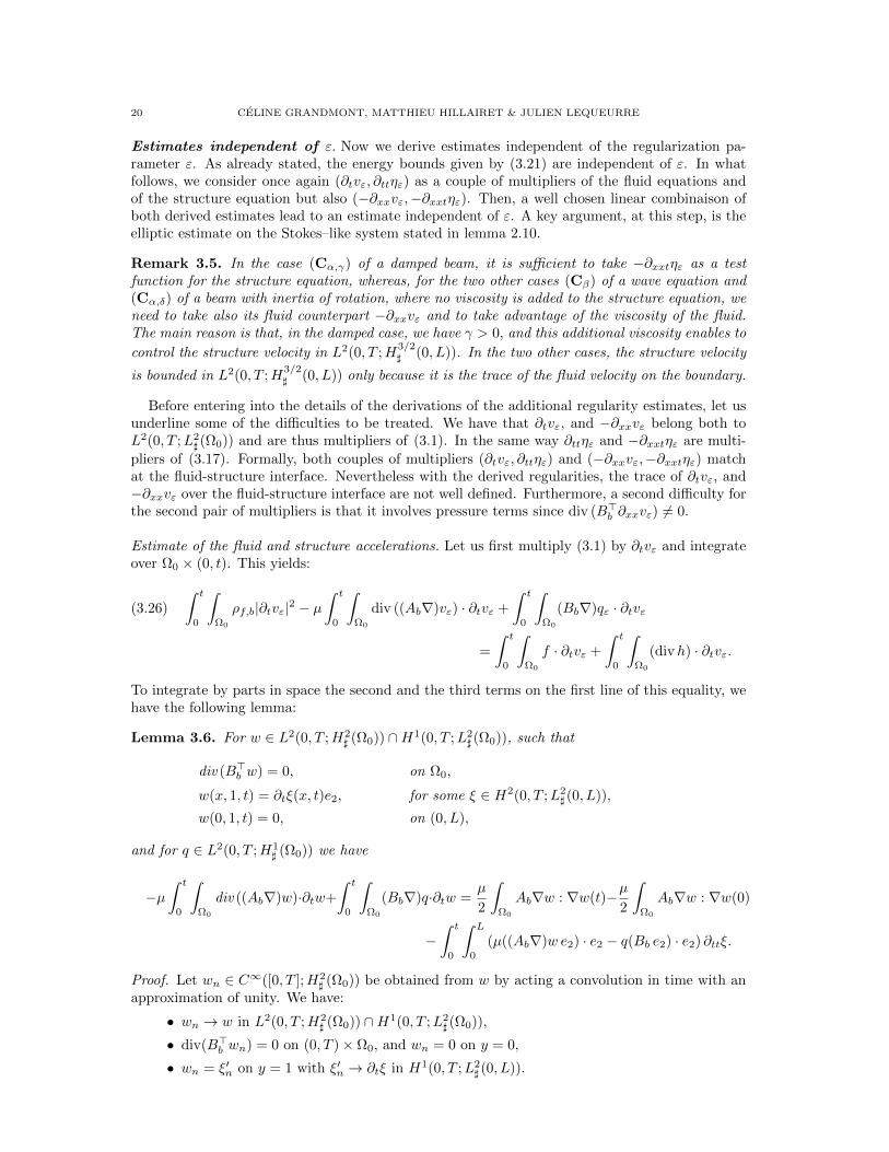
Estimates independent of ε. Now we derive estimates independent of the regularization pa-rameter ε. As already stated, the energy bounds given by (3.21) are independent of ε. In whatfollows, we consider once again (∂tvε, ∂ttηε) as a couple of multipliers of the fluid equations andof the structure equation but also (−∂xxvε,−∂xxtηε). Then, a well chosen linear combinaison ofboth derived estimates lead to an estimate independent of ε. A key argument, at this step, is theelliptic estimate on the Stokes–like system stated in lemma 2.10.

Remark 3.5. In the case (Cα,γ) of a damped beam, it is sufficient to take −∂xxtηε as a testfunction for the structure equation, whereas, for the two other cases (Cβ) of a wave equation and(Cα,δ) of a beam with inertia of rotation, where no viscosity is added to the structure equation, weneed to take also its fluid counterpart −∂xxvε and to take advantage of the viscosity of the fluid.The main reason is that, in the damped case, we have γ > 0, and this additional viscosity enables to

control the structure velocity in L2(0, T ;H3/2] (0, L)). In the two other cases, the structure velocity

is bounded in L2(0, T ;H3/2] (0, L)) only because it is the trace of the fluid velocity on the boundary.

Before entering into the details of the derivations of the additional regularity estimates, let usunderline some of the difficulties to be treated. We have that ∂tvε, and −∂xxvε belong both toL2(0, T ;L2

] (Ω0)) and are thus multipliers of (3.1). In the same way ∂ttηε and −∂xxtηε are multi-

pliers of (3.17). Formally, both couples of multipliers (∂tvε, ∂ttηε) and (−∂xxvε,−∂xxtηε) matchat the fluid-structure interface. Nevertheless with the derived regularities, the trace of ∂tvε, and−∂xxvε over the fluid-structure interface are not well defined. Furthermore, a second difficulty forthe second pair of multipliers is that it involves pressure terms since div (B>b ∂xxvε) 6= 0.

Estimate of the fluid and structure accelerations. Let us first multiply (3.1) by ∂tvε and integrateover Ω0 × (0, t). This yields:

(3.26)

∫ t

0

∫Ω0

ρf,b|∂tvε|2 − µ∫ t

0

∫Ω0

div ((Ab∇)vε) · ∂tvε +

∫ t

0

∫Ω0

(Bb∇)qε · ∂tvε

=

∫ t

0

∫Ω0

f · ∂tvε +

∫ t

0

∫Ω0

(divh) · ∂tvε.

To integrate by parts in space the second and the third terms on the first line of this equality, wehave the following lemma:

Lemma 3.6. For w ∈ L2(0, T ;H2] (Ω0)) ∩H1(0, T ;L2

] (Ω0)), such that

div (B>b w) = 0, on Ω0,

w(x, 1, t) = ∂tξ(x, t)e2, for some ξ ∈ H2(0, T ;L2] (0, L)),

w(0, 1, t) = 0, on (0, L),

and for q ∈ L2(0, T ;H1] (Ω0)) we have

−µ∫ t

0

∫Ω0

div ((Ab∇)w)·∂tw+

∫ t

0

∫Ω0

(Bb∇)q·∂tw =µ

2

∫Ω0

Ab∇w : ∇w(t)−µ2

∫Ω0

Ab∇w : ∇w(0)

−∫ t

0

∫ L

0

(µ((Ab∇)w e2) · e2 − q(Bb e2) · e2) ∂ttξ.

Proof. Let wn ∈ C∞([0, T ];H2] (Ω0)) be obtained from w by acting a convolution in time with an

approximation of unity. We have:

• wn → w in L2(0, T ;H2] (Ω0)) ∩H1(0, T ;L2

] (Ω0)),

• div(B>b wn) = 0 on (0, T )× Ω0, and wn = 0 on y = 0,

• wn = ξ′n on y = 1 with ξ′n → ∂tξ in H1(0, T ;L2] (0, L)).


For such a regular vector-field wn, the identity under consideration is a simple integration by parts.We note then that, since (Ab, Bb) ∈ L∞((0, T );L∞] (Ω0)) with

supy∈(0,1)

‖∇Ab‖L2](0,L) <∞.

and L2(0, T ;H2] (Ω0))∩H1(0, T ;L2

] (Ω0)) embeds in C([0, T ];H1] (Ω0)), all the integrals involved in

this identity are continuous with respect to the topology for which wn and ξ′n converge. This endsthe proof.

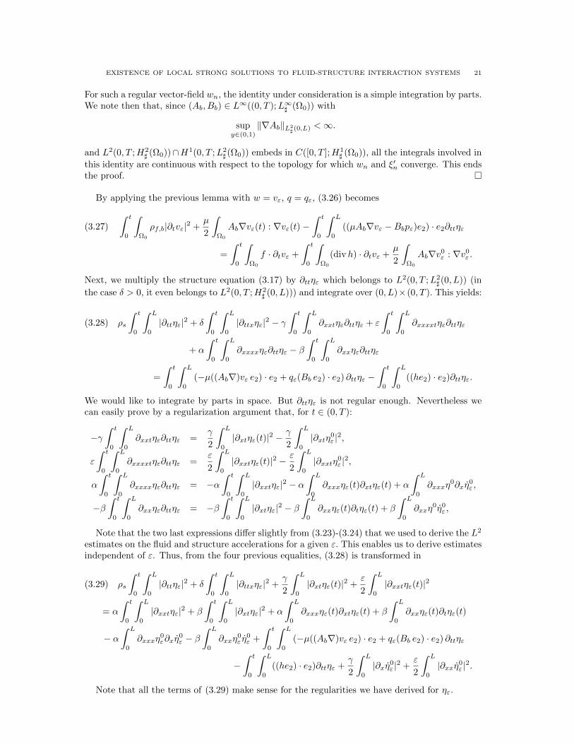
By applying the previous lemma with w = vε, q = qε, (3.26) becomes

(3.27)

∫ t

0

∫Ω0

ρf,b|∂tvε|2 +µ

2

∫Ω0

Ab∇vε(t) : ∇vε(t)−∫ t

0

∫ L

0

((µAb∇vε −Bbpε)e2) · e2∂ttηε

=

∫ t

0

∫Ω0

f · ∂tvε +

∫ t

0

∫Ω0

(divh) · ∂tvε +µ

2

∫Ω0

Ab∇v0ε : ∇v0

ε .

Next, we multiply the structure equation (3.17) by ∂ttηε which belongs to L2(0, T ;L2] (0, L)) (in

the case δ > 0, it even belongs to L2(0, T ;H2] (0, L))) and integrate over (0, L)×(0, T ). This yields:

(3.28) ρs

∫ t

0

∫ L

0

|∂ttηε|2 + δ

∫ t

0

∫ L

0

|∂ttxηε|2 − γ∫ t

0

∫ L

0

∂xxtηε∂ttηε + ε

∫ t

0

∫ L

0

∂xxxxtηε∂ttηε

+ α

∫ t

0

∫ L

0

∂xxxxηε∂ttηε − β∫ t

0

∫ L

0

∂xxηε∂ttηε

=

∫ t

0

∫ L

0

(−µ((Ab∇)vε e2) · e2 + qε(Bb e2) · e2) ∂ttηε −∫ t

0

∫ L

0

((he2) · e2)∂ttηε.

We would like to integrate by parts in space. But ∂ttηε is not regular enough. Nevertheless wecan easily prove by a regularization argument that, for t ∈ (0, T ):

−γ∫ t

0

∫ L

0

∂xxtηε∂ttηε =γ

2

∫ L

0

|∂xtηε(t)|2 −γ

2

∫ L

0

|∂xtη0ε |2,

ε

∫ t

0

∫ L

0

∂xxxxtηε∂ttηε =ε

2

∫ L

0

|∂xxtηε(t)|2 −ε

2

∫ L

0

|∂xxtη0ε |2,

α

∫ t

0

∫ L

0

∂xxxxηε∂ttηε = −α∫ t

0

∫ L

0

|∂xxtηε|2 − α∫ L

0

∂xxxηε(t)∂xtηε(t) + α

∫ L

0

∂xxxη0∂xη

0ε ,

−β∫ t

0

∫ L

0

∂xxηε∂ttηε = −β∫ t

0

∫ L

0

|∂xtηε|2 − β∫ L

0

∂xxηε(t)∂tηε(t) + β

∫ L

0

∂xxη0η0ε ,

Note that the two last expressions differ slightly from (3.23)-(3.24) that we used to derive the L2

estimates on the fluid and structure accelerations for a given ε. This enables us to derive estimatesindependent of ε. Thus, from the four previous equalities, (3.28) is transformed in

(3.29) ρs

∫ t

0

∫ L

0

|∂ttηε|2 + δ

∫ t

0

∫ L

0

|∂ttxηε|2 +γ

2

∫ L

0

|∂xtηε(t)|2 +ε

2

∫ L

0

|∂xxtηε(t)|2

= α

∫ t

0

∫ L

0

|∂xxtηε|2 + β

∫ t

0

∫ L

0

|∂xtηε|2 + α

∫ L

0

∂xxxηε(t)∂xtηε(t) + β

∫ L

0

∂xxηε(t)∂tηε(t)

− α∫ L

0

∂xxxη0ε∂xη

0ε − β

∫ L

0

∂xxη0ε η

0ε +

∫ t

0

∫ L

0

(−µ((Ab∇)vε e2) · e2 + qε(Bb e2) · e2) ∂ttηε

−∫ t

0

∫ L

0

((he2) · e2)∂ttηε +γ

2

∫ L

0

|∂xη0ε |2 +

ε

2

∫ L

0

|∂xxη0ε |2.

Note that all the terms of (3.29) make sense for the regularities we have derived for ηε.


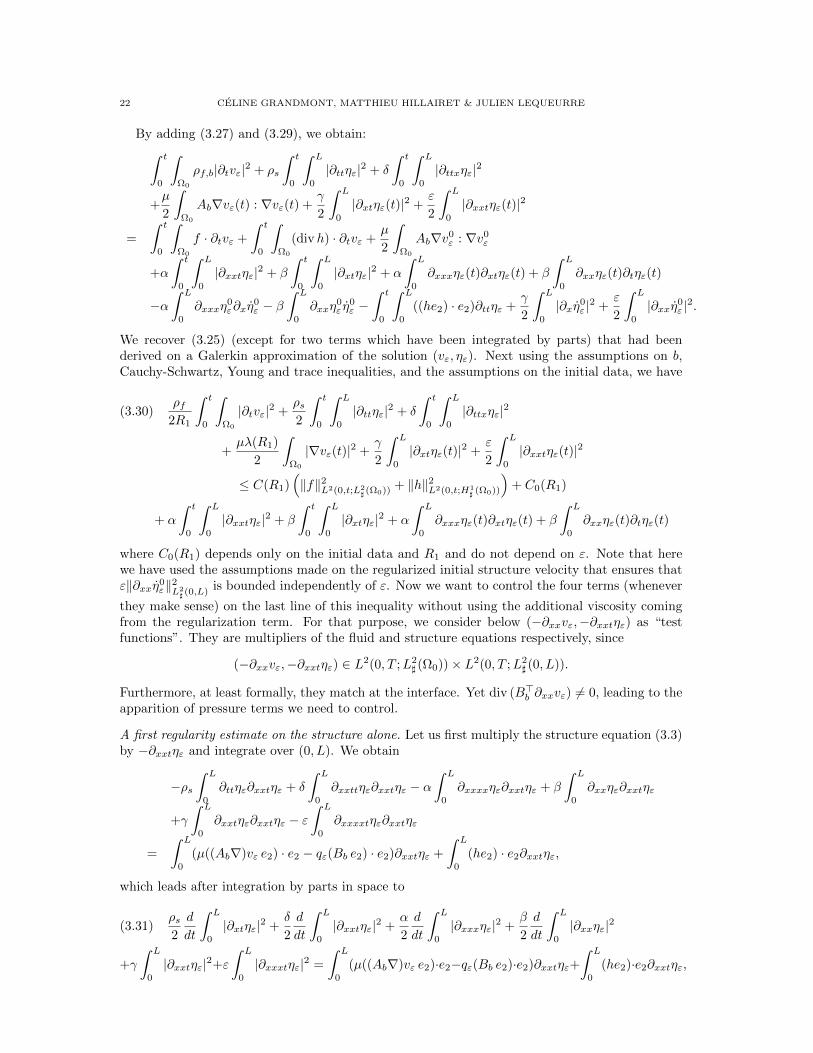
By adding (3.27) and (3.29), we obtain:∫ t

0

∫Ω0


∫ t

0

∫ L

0

|∂ttηε|2 + δ

∫ t

0

∫ L

0

|∂ttxηε|2

+µ

2

∫Ω0

Ab∇vε(t) : ∇vε(t) +γ

2

∫ L

0

|∂xtηε(t)|2 +ε

2

∫ L

0

|∂xxtηε(t)|2

=

∫ t

0

∫Ω0

f · ∂tvε +

∫ t

0

∫Ω0

(divh) · ∂tvε +µ

2

∫Ω0

Ab∇v0ε : ∇v0

ε

+α

∫ t

0

∫ L

0

|∂xxtηε|2 + β

∫ t

0

∫ L

0

|∂xtηε|2 + α

∫ L

0


∫ L

0


−α∫ L

0

∂xxxη0ε∂xη

0ε − β

∫ L

0

∂xxη0ε η

0ε −

∫ t

0

∫ L

0

((he2) · e2)∂ttηε +γ

2

∫ L

0

|∂xη0ε |2 +

ε

2

∫ L

0

|∂xxη0ε |2.

We recover (3.25) (except for two terms which have been integrated by parts) that had beenderived on a Galerkin approximation of the solution (vε, ηε). Next using the assumptions on b,Cauchy-Schwartz, Young and trace inequalities, and the assumptions on the initial data, we have

(3.30)ρf

2R1

∫ t

0

∫Ω0

|∂tvε|2 +ρs2

∫ t

0

∫ L

0

|∂ttηε|2 + δ

∫ t

0

∫ L

0

|∂ttxηε|2

+µλ(R1)

2

∫Ω0

|∇vε(t)|2 +γ

2

∫ L

0

|∂xtηε(t)|2 +ε

2

∫ L

0

|∂xxtηε(t)|2

≤ C(R1)(‖f‖2L2(0,t;L2

](Ω0)) + ‖h‖2L2(0,t;H1] (Ω0))

)+ C0(R1)

+ α

∫ t

0

∫ L

0

|∂xxtηε|2 + β

∫ t

0

∫ L

0

|∂xtηε|2 + α

∫ L

0


∫ L

0


where C0(R1) depends only on the initial data and R1 and do not depend on ε. Note that herewe have used the assumptions made on the regularized initial structure velocity that ensures thatε‖∂xxη0

ε‖2L2](0,L)

is bounded independently of ε. Now we want to control the four terms (whenever

they make sense) on the last line of this inequality without using the additional viscosity comingfrom the regularization term. For that purpose, we consider below (−∂xxvε,−∂xxtηε) as “testfunctions”. They are multipliers of the fluid and structure equations respectively, since

(−∂xxvε,−∂xxtηε) ∈ L2(0, T ;L2] (Ω0))× L2(0, T ;L2

] (0, L)).

Furthermore, at least formally, they match at the interface. Yet div (B>b ∂xxvε) 6= 0, leading to theapparition of pressure terms we need to control.

A first regularity estimate on the structure alone. Let us first multiply the structure equation (3.3)by −∂xxtηε and integrate over (0, L). We obtain

−ρs∫ L

0

∂ttηε∂xxtηε + δ

∫ L

0

∂xxttηε∂xxtηε − α∫ L

0

∂xxxxηε∂xxtηε + β

∫ L

0

∂xxηε∂xxtηε

+γ

∫ L

0

∂xxtηε∂xxtηε − ε∫ L

0

∂xxxxtηε∂xxtηε

=

∫ L

0

(µ((Ab∇)vε e2) · e2 − qε(Bb e2) · e2)∂xxtηε +

∫ L

0

(he2) · e2∂xxtηε,

which leads after integration by parts in space to

(3.31)ρs2

d

dt

∫ L

0

|∂xtηε|2 +δ

2

d

dt

∫ L

0

|∂xxtηε|2 +α

2

d

dt

∫ L

0

|∂xxxηε|2 +β

2

d

dt

∫ L

0

|∂xxηε|2

+γ

∫ L

0

|∂xxtηε|2+ε

∫ L

0

|∂xxxtηε|2 =

∫ L

0

(µ((Ab∇)vε e2)·e2−qε(Bb e2)·e2)∂xxtηε+

∫ L

0

(he2)·e2∂xxtηε,


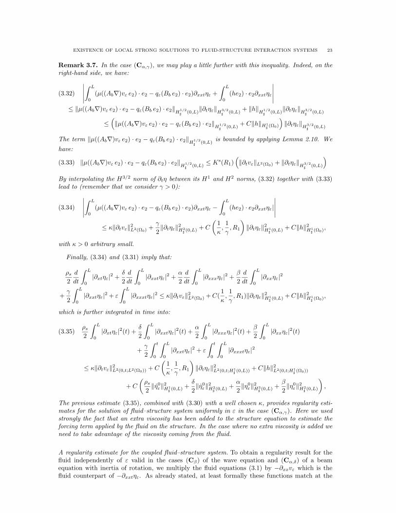
Remark 3.7. In the case (Cα,γ), we may play a little further with this inequality. Indeed, on theright-hand side, we have:

(3.32)

∣∣∣∣∣∫ L

0

(µ((Ab∇)vε e2) · e2 − qε(Bb e2) · e2)∂xxtηε +

∫ L

0

(he2) · e2∂xxtηε

∣∣∣∣∣≤ ‖µ((Ab∇)vε e2) · e2 − qε(Bb e2) · e2‖H1/2

] (0,L)‖∂tηε‖H3/2

] (0,L)+ ‖h‖

H1/2] (0,L)

‖∂tηε‖H3/2] (0,L)

≤(‖µ((Ab∇)vε e2) · e2 − qε(Bb e2) · e2‖H1/2

] (0,L)+ C‖h‖H1

] (Ω0)

)‖∂tηε‖H3/2

] (0,L)

The term ‖µ((Ab∇)vε e2) · e2 − qε(Bb e2) · e2‖H1/2] (0,L)

is bounded by applying Lemma 2.10. We

have:

(3.33) ‖µ((Ab∇)vε e2) · e2 − qε(Bb e2) · e2‖H1/2] (0,L)

≤ Ks(R1)(‖∂tvε‖L2(Ω0) + ‖∂tηε‖H3/2

] (0,L)

)By interpolating the H3/2 norm of ∂tη between its H1 and H2 norms, (3.32) together with (3.33)lead to (remember that we consider γ > 0):

(3.34)

∣∣∣∣∣∫ L

0

(µ((Ab∇)vε e2) · e2 − qε(Bb e2) · e2)∂xxtηε −∫ L

0

(he2) · e2∂xxtηε|

∣∣∣∣∣≤ κ‖∂tvε‖2L2(Ω0) +

γ

2‖∂tηε‖2H2

] (0,L) + C

(1

κ,

1

γ,R1

)‖∂tηε‖2H1

] (0,L) + C‖h‖2H1] (Ω0),

with κ > 0 arbitrary small.

Finally, (3.34) and (3.31) imply that:

ρs2

d

dt

∫ L

0

|∂xtηε|2 +δ

2

d

dt

∫ L

0

|∂xxtηε|2 +α

2

d

dt

∫ L

0

|∂xxxηε|2 +β

2

d

dt

∫ L

0

|∂xxηε|2

+γ

2

∫ L

0

|∂xxtηε|2 + ε

∫ L

0

|∂xxxtηε|2 ≤ κ‖∂tvε‖2L2(Ω0) +C(1

κ,

1

γ,R1)‖∂tηε‖2H1

] (0,L) +C‖h‖2H1] (Ω0),

which is further integrated in time into:

(3.35)ρs2

∫ L

0

|∂xtηε|2(t) +δ

2

∫ L

0

|∂xxtηε|2(t) +α

2

∫ L

0

|∂xxxηε|2(t) +β

2

∫ L

0

|∂xxηε|2(t)

+γ

2

∫ t

0

∫ L

0

|∂xxtηε|2 + ε

∫ t

0

∫ L

0

|∂xxxtηε|2

≤ κ‖∂tvε‖2L2(0,t;L2(Ω0)) + C

(1

κ,

1

γ,R1

)‖∂tηε‖2L2(0,t;H1

] (0,L)) + C‖h‖2L2(0,t;H1] (Ω0))

+ C

(ρs2‖η0ε‖2H1

] (0,L) +δ

2‖η0ε‖2H2

] (0,L) +α

2‖η0ε‖2H3

] (0,L) +β

2‖η0ε‖2H2

] (0,L)

),

The previous estimate (3.35), combined with (3.30) with a well chosen κ, provides regularity esti-mates for the solution of fluid–structure system uniformly in ε in the case (Cα,γ). Here we usedstrongly the fact that an extra viscosity has been added to the structure equation to estimate theforcing term applied by the fluid on the structure. In the case where no extra viscosity is added weneed to take advantage of the viscosity coming from the fluid.

A regularity estimate for the coupled fluid–structure system. To obtain a regularity result for thefluid independently of ε valid in the cases (Cβ) of the wave equation and (Cα,δ) of a beamequation with inertia of rotation, we multiply the fluid equations (3.1) by −∂xxvε which is thefluid counterpart of −∂xxtηε. As already stated, at least formally these functions match at the


interface. We have,

−∫ t

0

∫Ω0

ρf,b∂tvε · ∂xxvε +

∫ t

0

∫Ω0

(µdiv ((Ab∇)vε)− (Bb∇)qε) · ∂xxvε =

−∫ t

0

∫Ω0

f · ∂xxvε −∫ t

0

∫Ω0

divh · ∂xxvε.

At this stage we remark that −∂xxvε is not regular enough to perform the desired integrationby parts and moreover −∂xxvε does not satisfied div (B>b ∂xxvε) = 0. Nevertheless the followinglemma holds true

Lemma 3.8. For w ∈ L2(0, T ;H2] (Ω0)) ∩H1(0, T ;L2

] (Ω0)), such that

w(x, 1, t) = ∂tξ(x, t)e2, for some ξ ∈ H1(0, T ;H2] (0, L)),

w(x, 0, t) = 0, on (0, L),

and for q ∈ L2(0, T ;H1] (Ω0)) we have

−∫ t

0

∫Ω0

ρf,b∂tw · ∂xxw +

∫ t

0

∫Ω0

(µdiv ((Ab∇)w)− (Bb∇)q) · ∂xxw

=1

2

∫Ω0

ρf,b|∂xw|2(t)− 1

2

∫Ω0

ρf,b|∂xw|2(0) +

∫ t

0

∫Ω0

ρf∂xb ∂tw · ∂xw

+

∫ t

0

⟨µ((Ab∇)w e2) · e2 − q(Bb e2) · e2, ∂xxtξ

⟩H

12] (0,L),H

− 12

] (0,L)+ µ

∫ t

0

∫Ω0

Ab∇∂xw : ∇∂xw

+µ

∫ t

0

∫Ω0

(∂xAb∇)w : ∇∂xw −∫ t

0

∫Ω0

∂xq Bb : ∇∂xw −∫ t

0

∫Ω0

q ∂xBb : ∇∂xw.

Moreover if div (B>b w) = 0 then∫ t

0

∫Ω0

∂xq Bb : ∇∂xw = −∫ t

0

∫Ω0

∂xq ∂xBb : ∇w.

Proof. By convolution (in time and space), we can approximate w by a family (wn)n∈N of smoothvector-fields such that:

wn → w in L2(0, T ;H2] (0, L)) ∩H1(0, T ;L2

] (Ω0))

We have then that, when n→∞, the following convergences hold:

wn → 0 in L2(0, T ;H3/2] (0, L)) so that ∂xxwn → 0 in L2(0, T ;H

−1/2] (0, L)) on y = 0 ,

wn → ∂tξe2 in L2(0, T ;H3/2] (0, L)) so that ∂xxwn → ∂xxtξe2 in L2(0, T ;H

−1/2] (0, L)) on y = 1 ,

(Ab∇)wne2 → (Ab∇)we2 in L2(0, T ;H1/2] (0, L)) on y = 1 and y = 0.

Again, the identity to be proven is a simple integration by parts for wn. We may extend the identityto w by remarking that all integrals involved in these identities are continuous with respect to thetopology for which wn converges to w.

We apply the previous lemma for w = vε and we obtain

(3.36)1

2

∫Ω0

ρf,b|∂xvε|2(t) + µ

∫ t

0

∫Ω0

Ab∇∂xvε : ∇∂xvε

= −∫ t

0

∫ L

0

(µ((Ab∇)vε e2) · e2 − q(Bb e2) · e2) ∂xxtηε −∫ t

0

∫Ω0


0

∫Ω0

divh · ∂xxvε

+1

2

∫Ω0

ρf,b|∂xu0ε|2 −

∫ t

0

∫Ω0

ρf∂xb ∂tvε · ∂xvε − µ∫ t

0

∫Ω0

∂xAb∇vε : ∇∂xvε

+

∫ t

0

∫Ω0

∂xqεBb : ∇∂xvε +

∫ t

0

∫Ω0

qε ∂xBb : ∇∂xvε.


The forcing term involving h can be integrated by parts

−∫ t

0

∫Ω0

divh · ∂xxvε = −∫ t

0

∫Ω0

∂xh : ∇∂xvε −∫ t

0

∫ L

0

he2 · e2∂xxtηε.

From (3.36) we deduce

(3.37)

1

2

∫Ω0

ρf,b|∂xvε|2(t) + µ

∫ t

0

∫Ω0

Ab∇∂xvε : ∇∂xvε

= −∫ t

0

∫ L

0

(µ((Ab∇)vε e2) · e2 − qε(Bb e2) · e2) ∂xxtηε −∫ t

0

∫ L

0

he2 · e2∂xxtηε

−∫ t

0

∫Ω0


0

∫Ω0

∂xh : ∇∂xvε +1

2

∫Ω0

ρf,b|∂xu0ε|2

−∫ t

0

∫Ω0

ρf∂xb ∂tvε · ∂xvε − µ∫ t

0

∫Ω0

∂xAb∇vε : ∇∂xvε

+

∫ t

0

∫Ω0


∫ t

0

∫Ω0


The first (respectively the second) term in the right-hand side correspond to the forcing termapplied by the fluid on the structure (respectively to the external forcing term on the structure),namely the opposite of the first term (respectively the second term) in the right hand side of(3.31). By adding (3.37) and (3.31) (that has been previously integrated with respect to time)and by recalling that Ab ≥ λ(R1)I2, we thus obtain, after some rearrangement of the terms

(3.38)

Hr(t) + µλ(R1)

∫ t

0

∫Ω0

|∇∂xvε|2 + γ

∫ t

0

∫ L

0

|∂xxtηε|2 + ε

∫ t

0

∫ L

0

|∂xxxtηε|2

≤ H0r −

∫ t

0

∫Ω0


0

∫Ω0

∂xh · ∇∂xvε −∫ t

0

∫Ω0

ρf∂xb ∂tvε · ∂xvε

−∫ t

0

∫Ω0

µ(∂xAb∇)vε : ∇∂xvε +

∫ t

0

∫Ω0


∫ t

0

∫Ω0


where :

Hr(t) =1

2

∫Ω0

ρf,b|∂xvε|2(t) +ρs2

∫ L

0

|∂xtηε|2(t) +δ

2

∫ L

0

|∂xxtηε|2(t)

+α

2

∫ L

0

|∂xxxηε|2(t) +β

2

∫ L

0

|∂xxηε|2(t),

and H0r = Hr(0). To proceed with (3.38), we compute bounds for the right-hand side. The most

intricated terms are the four last ones on the right-hand side, which are the remainder termscoming from the derivation of the geometry with respect to x (and thus involving b). We denotethese terms Ti, i = 1, 2, 3, 4.

So, let us consider the right-hand side terms in their order of appearence in equation (3.38).First, for the initial conditions, we have

(3.39)1

2

∫Ω0

ρf,b|∂xu0ε|2 +

ρs2

∫ L

0

|∂xη0ε |2 +

δ

2

∫ L

0

|∂xxη0ε |2 +

α

2

∫ L

0

|∂xxxη0ε |2 +

β

2

∫ L

0

|∂xxη0ε |2

≤ C ρfR1

2‖v0ε‖2H1

] (Ω0) +ρs2‖η0ε‖2H1

] (0,L) +δ

2‖η0ε‖2H2

] (0,L) +α

2‖η0ε‖2H3

] (0,L) +β

2‖η0ε‖2H2

] (0,L).

Due to our assumptions on initial data, this last right-hand side is bounded whatever the value of(α, β, γ, δ) in the three different cases under consideration. Then, the external forcing terms are


bounded with classical inequalities:

(3.40)

∣∣∣∣∫ t

0

∫Ω0

f · ∂xxvε +

∫ t

0

∫Ω0

∂xh · ∇∂xvε∣∣∣∣ ≤ ∫ t

0

(‖f‖L2

](Ω0) + ‖h‖H1] (Ω0)

)‖∇∂xvε‖L2

](Ω0)

≤ C(R1,

1

µ

)(‖f‖2L2(0,t;L2

](Ω0)) + ‖h‖2L2(0,t;H1] (Ω0))

)+µλ(R1)

16‖∇∂xvε‖2L2(0,t;L2

](Ω0))

We turn now to the geometrical terms Ti. The first one is given by

T1 = −∫ t

0

∫Ω0

ρfbx ∂tvε · ∂xvε.

We recall that b ∈ H2] (0, L) ⊂ C1([0, L]). Then, classically, we have that, for κ > 0 to be fixed

later,

(3.41) |T1| ≤ κ‖∂tvε‖2L2(0,t;L2](Ω0)) + C

(ρf , R1,

1

κ

)‖∇vε‖2L2(0,t;L2

](Ω0)).

Note that ‖vε‖2L2(0,t;H1] (Ω0))

is bounded independently of ε thanks to the energy estimate (3.20).

The second term is defined by

T2 = −∫ t

0

∫Ω0

∂xAb∇vε : ∇∂xvε,

As we stated previously (∂xAb, ∂xBb) ∈ L2] ((0, L), Hs(0, 1)), for arbitrary s ≥ 0, (with norms

bounded by a function of R1) and H1] ((0, L) × (0, 1)) ⊂ L∞] ((0, L);L2(0, 1)). Hence, in the spirit

of [13, Lemma 6] and of the proof of Lemma 2.10 (that can be found in [15]), we bound T2 asfollows(3.42)

|T2| ≤ C

∫ t

0

‖∂xAb‖L∞(0,1;L2](0,L))‖∇vε‖L2(0,1;L∞] (0,L))‖∇∂xvε‖L2

](Ω0)

≤∫ t

0

‖∂xAb‖L∞(0,1;L2](0,L))

[‖∇vε‖1/2L2

](Ω0)‖∇∂xvε‖3/2L2

](Ω0)+ ‖∇vε‖L2

](Ω0)‖∇∂xvε‖L2](Ω0)

]≤ C

(R1,

1

µ

)‖∇vε‖2L2(0,t;L2

](Ω0)) +µλ(R1)

8‖∇∂xvε‖2L2(0,t;L2

](Ω0)).

The first term in the right hand side is bounded independently of ε thanks to the energy estimate(3.20) and the second term can be absorbed by the second term of (3.38).

The two last terms involve the pressure for which we have no bound so far. Consequently weneed, at this step, to use Lemma 2.10 on ellipticity of the Stokes-like problem. The third term isdefined by

T3 =

∫ t

0

∫Ω0

∂xqεBb : ∇∂xvε.

As stated in Lemma 3.8, T3 reads:

T3 = −∫ t

0

∫Ω0

∂xqε ∂xBb : ∇vε.

Once again, following the same lines as in [13, Lemma 6] and in the proof of Lemma 2.10 (see[15]), we obtain

|T3| ≤∫ t

0

‖∂xqε‖L2](Ω0)‖∂xBb : ∇vε‖L2

](Ω0),

≤ C(R1)

∫ t

0

‖∂xqε‖L2](Ω0)

[‖∇vε‖1/2L2

](Ω0)‖∇∂xvε‖1/2L2

](Ω0)+ ‖∇vε‖L2

](Ω0)

].


Using the elliptic result of Lemma 2.10, and the equality of the fluid and structure velocities at

the interface, we have (since ∂tηε ∈ H32

] (0, L) ∩ L2],0(0, L)):

‖∂xqε‖L2](Ω0) ≤ Ks(R1)

(‖∂tvε‖L2

](Ω0) + ‖∂txηε‖H1/2] (0,L)

)≤ Ks(R1)

(‖∂tvε‖L2

](Ω0) + ‖∂xvε‖H1] (Ω0)

).

Therefore, we have the bound:

(3.43) |T3| ≤ κ‖∂tvε‖2L2(0,t;L2(Ω0)) +µλ(R1)

8‖∇∂xvε‖2L2(0,t;L2

](Ω0))

+ C

(R1,

1

µ,

1

κ

)‖∇vε(t)‖2L2(0,t;L2

](Ω0)).

The last term T4 is

T4 =

∫ t

0

∫Ω0


At this point, we note that ∂xBb ∈ L∞(0, 1;L2] (0, L)), ∇∂xvε ∈ L2(0, T ;L2

] (Ω0)) and qε ∈L2(0, T ;H1

] (Ω0)) ⊂ L2(0, T ;L2(0, 1;L∞] (0, L))). Hence, again with the same trick of tensorizingthe space-integral, we have that T4 is well-defined and a continuous mapping of its argument inthe mentioned spaces. Up to an approximation argument, we may thus assume that b ∈ C∞] (0, L)

so that Bb ∈ C∞] (Ω0). Then, since div (Bb) = 0 due to Piola identity we have div (∂xBb) = 0.Consequently, we have:

T4 = −∫ t

0

∫Ω0

∇qε ∂xB>b ∂xvε +

∫ t

0

∫ L

0

[qε∂xB>b ∂xvε · e2(x, 1)]|y=1

dx.

The first term can be estimated exactly as T3:

(3.44)

∣∣∣∣∫ t

0

∫Ω0

∇qε ∂xB>b ∂xvε∣∣∣∣ ≤ κ‖∂tvε‖2L2(0,t;L2(Ω0)) +

µλ(R1)

8‖∇∂xvε‖2L2(0,t;L2

](Ω0))

+C

(R1,

1

µ,

1

κ

)‖∇vε‖2L2(0,t;L2

](Ω0))

As for the boundary term, because the change of variables χb maps Ω0 to Ωb, we have in particular,thanks to the Nanson formula in (0, L) that

Bbe2 = −∂xbe1 + e2,

therefore, we obtain ∂x(Bbe2) = −∂xxbe1. On the other hand, the boundary condition at theinterface fluid/structure, that is for x ∈ (0, L) is vε(t, x, 1) = ∂tηε(t, x)e2, which makes sense in

L2(0, T ;H3/2] (Ω0)) therefore, we obtain ∂xvε(t, x) = ∂txηε(t, x)e2 in L2(0, T ;H

1/2] (Ω0)). Thus, we

have

∂xBbe2 · ∂xvε = 0 in L2(0, T ;H1/2(0, L)).

and finally, the boundary integral is thus zero. Then, from (3.44), we deduce

(3.45) |T4| ≤ κ‖∂tvε‖2L2(0,t;L2(Ω0)) +µλ(R1)

8‖∇∂xvε‖2L2(0,t;L2

](Ω0))

+ C

(R1,

1

µ,

1

κ

)‖∇vε‖2L2(0,t;L2

](Ω0)).


Consequently, from (3.38), and taking into account (3.40), (3.39), (3.41), (3.42), (3.43), (3.45),we end up with

(3.46)

1

2

∫Ω0

ρf,b|∂xvε|2(t)+ρs2

∫ L

0

|∂xtηε|2(t)+δ

2

∫ L

0

|∂xxtηε|2(t)+α

2

∫ L

0

|∂xxxηε|2(t)+β

2

∫ L

0

|∂xxηε|2(t)

+µλ(R1)

2

∫ t

0

∫Ω0

|∇∂xvε|2 + γ

∫ t

0

∫ L

0

|∂xxtηε|2 + ε

∫ t

0

∫ L

0

|∂xxxtηε|2

≤ 4κ‖∂tvε‖2L2(0,t;L2](Ω0)) + C(ρf , R1,

1

µ,

1

κ)(‖f‖2L2(0,t;L2

](Ω0)) + ‖h‖2L2(0,t;H1] (Ω0))

+ρf‖u0‖2H1] (Ω0) +

ρs2‖η0‖2H1

] (0,L) +δ

2‖η0‖2H2

] (0,L) +α

2‖η0‖2H3

] (0,L) +β

2‖η0‖2H2

] (0,L)

),

Final regularity estimates. We are now in a position to close a regularity estimate independent ofthe parameter of regularization ε. We recall that, until now, we obtained two inequalities. Thefirst one, (3.30) is obtained by taking (∂tvε, ∂ttηε) as test functions. It reads:

ρf2R1

∫ t

0

∫Ω0

|∂tvε|2 +ρs2

∫ t

0

∫ L

0

|∂ttηε|2 + δ

∫ t

0

∫ L

0

|∂ttxηε|2

+µλ(R1)

2

∫Ω0

|∇vε(t)|2 +γ

2

∫ L

0

|∂xtηε(t)|2 +ε

2

∫ L

0

|∂xxtηε(t)|2

≤ C(R1)(‖f‖2L2(0,t;L2

](Ω0)) + ‖h‖2L2(0,t;H1] (Ω0))

)+ C0(R1)

+ α

∫ t

0

∫ L

0

|∂xxtηε|2 + β

∫ t

0

∫ L

0

|∂xtηε|2 + α

∫ L

0


∫ L

0


Second, we have the above coupled regularity estimate (3.46):

1

2

∫Ω0


∫ L

0

|∂xtηε|2(t)+δ

2

∫ L

0

|∂xxtηε|2(t)+α

2

∫ L

0

|∂xxxηε|2(t)+β

2

∫ L

0

|∂xxηε|2(t)

+µλ(R1)

2

∫ t

0

∫Ω0

|∇∂xvε|2 + γ

∫ t

0

∫ L

0

|∂xxtηε|2 + ε

∫ t

0

∫ L

0

|∂xxxtηε|2

≤ 4κ‖∂tvε‖2L2(0,t;L2](Ω0)) + C(ρf , R1,

1

µ,

1

κ)(‖f‖2L2(0,t;L2

](Ω0)) + ‖h‖2L2(0,t;H1] (Ω0))

+ρf‖u0‖2H1] (Ω0) +

ρs2‖η0‖2H1

] (0,L) +δ

2‖η0‖2H2

] (0,L) +α

2‖η0‖2H3

] (0,L) +β

2‖η0‖2H2

] (0,L)

),

We propose to write the combination (EΛ) = Λ(3.30)+(3.46) with a parameter Λ that we fixbelow. On the right-hand side of this inequality, we obtain then at most 5 terms to bound:

I1 := Λα

∫ t

0

∫ L

0

|∂xxtηε|2 I2 := Λβ

∫ t

0

∫ L

0

|∂xtηε|2

I3 := Λα

∫ L

0

∂xxxηε(t)∂xtηε(t) I4 := Λβ

∫ L

0


I5 := 4κ

∫ t

0

∫Ω0

|∂tvε|2

First, we restrict Λ to satisfy Λα ≤ (γ+ δ)/2 (we remind that, with our assumptions, if γ = δ = 0then α = 0 so that this inequality is not a restriction on Λ in this case). We may then bound:

I1 ≤γ + δ

2

∫ t

0

∫ L

0

|∂xxtηε|2,


Second, we restrict Λ to satisfy Λ ≤ 1/2 and Λα ≤ ρs/4. We have then:

I3 ≤α

4

∫ L

0

|∂xxxηε|2(t) +ρs8

∫ L

0

|∂xtηε(t)|2

Finally, we introduce CPW the optimal constant for the Poincare-Wirtinger in H1] (0, L)∩L2

],0(0, L).

We restrict then Λ to satisfy Λ|CPW |2β ≤ ρs/4. We obtain then (since ∂tη ∈ H1] (0, L)∩L2

],0(0, L)

for a.e. t ∈ (0, T ) and Λ ≤ 1/2):

I4 ≤β

4

∫ L

0

|∂xxηε(t)|2 +ρs8

∫ L

0

|∂xtηε(t)|2

Finally, we choose (with the convention that if 0 appears as a denominator of a fraction of the liston right-hand side, then the quantity must be deleted from the list):

Λ = min

(γ + δ

2α,

1

2,ρs4α,

ρs4|CPW |2β

)With this choice, we note that Λ > 0 so that we may choose

κ =ρf

16ΛR1.

Taking into account the bounds for I1, I3, I4 mentioned above, we have that the combination (EΛ)implies:

Λρf4R1

∫ t

0

∫Ω0

|∂tvε|2 +Λρs

2

∫ t

0

∫ L

0

|∂ttηε|2 + δΛ

∫ t

0

∫ L

0

|∂ttxηε|2

+1

2

∫Ω0


∫ L

0

|∂xtηε|2(t)+δ

2

∫ L

0

|∂xxtηε|2(t)+α

4

∫ L

0

|∂xxxηε|2(t)+β

4

∫ L

0

|∂xxηε|2(t)

+µΛλ(R1)

2

∫Ω0

|∇vε(t)|2 +Λγ

2

∫ L

0

|∂xtηε(t)|2 +Λε

2

∫ L

0

|∂xxtηε(t)|2

+µλ(R1)

2

∫ t

0

∫Ω0

|∇∂xvε|2 +γ

2

∫ t

0

∫ L

0

|∂xxtηε|2 + ε

∫ t

0

∫ L

0

|∂xxxtηε|2

≤ C(ρf , ρs, R1,

1

µ,

1

α,

1

β, γ, δ

)(‖f‖2L2(0,t;L2

](Ω0)) + ‖h‖2L2(0,t;H1] (Ω0))

+ρf‖u0‖2H1] (Ω0) +

ρs2‖η0‖2H1

] (0,L) +δ

2‖η0‖2H2

] (0,L) +α

2‖η0‖2H3

] (0,L) +β

2‖η0‖2H2

] (0,L)

),

+δ

2

∫ t

0

∫ T

0

|∂xxtηε|2 + Λβ

∫ t

0

∫ T

0

|∂xtηε|2.

We skip the dependencies of the constant C and we denote by C0 the quantity involving initialdata on the right-hand side to lighten notations. Finally, we remark that, by keeping all thenecessary terms, the quantity:

Y (t) =δ

2

∫ L

0

|∂xxtηε|2 +ρs4

∫ t

0

∫ L

0

|∂xtηε|2,

satisfies the Gronwall-type inequality:

Y (t) ≤ C(‖f‖2L2(0,T ;L2

](Ω0)) + ‖h‖2L2(0,T ;H1] (Ω0)) + C0

)+

(1 +

4Λβ

ρs

)∫ t

0

Y (s)ds

We obtain thus that:

Y (t) ≤ C(C0 + ‖f‖2L2(0,T ;L2

](Ω0)) + ‖h‖2L2(0,T ;H1] (Ω0))

)exp

[(1 +

4Λβ

ρs

)t

]∀ t > 0.


We may plug this inequality in (EΛ) to get, under the restriction that T < 1 :

Λρf4R1

∫ t

0

∫Ω0

|∂tvε|2 +Λρs

2

∫ t

0

∫ L

0

|∂ttηε|2 + δΛ

∫ t

0

∫ L

0

|∂ttxηε|2

+1

2

∫Ω0


∫ L

0

|∂xtηε|2(t)+δ

2

∫ L

0

|∂xxtηε|2(t)+α

4

∫ L

0

|∂xxxηε|2(t)+β

4

∫ L

0

|∂xxηε|2(t)

+µΛλ(R1)

2

∫Ω0

|∇vε(t)|2 +Λγ

2

∫ L

0

|∂xtηε(t)|2 +Λε

2

∫ L

0

|∂xxtηε(t)|2

+µλ(R1)

2

∫ t

0

∫Ω0

|∇∂xvε|2 +γ

2

∫ t

0

∫ L

0

|∂xxtηε|2 + ε

∫ t

0

∫ L

0

|∂xxxtηε|2

≤ C(C0 + ‖f‖2L2(0,T ;L2

](Ω0)) + ‖h‖2L2(0,T ;H1] (Ω0))

),

where C depends again only on ρf , ρs, R1, µ, α, β, γ, δ.

Limit as ε goes to zero and uniqueness. By strandard compactness arguments, we mayextract a weakly converging subsequence in the family of ε-solutions (ηε, vε, qε)ε>0. Applyingclassical arguments, we obtain that the weak limit (η, v, q) is a solution to our linear problemwith the expected regularity. Estimate (3.16) yields as the weak limit of the last inequality of theprevious section. All these computations are completly classical and left to the reader.

Finally, in the smooth-solution setting that we consider herein, we note that we can derive theenergy equality (3.19) by a multiplier argument. Consequently, if we were having two solutionsto (3.1)–(3.3) with the same data, the difference would satisfy (3.19) with vanishing data. Thisimplies that both solutions are equal: we have uniqueness of the solution to (3.1)–(3.3).

This ends the proof of Proposition 3.2

3.3. Non homogeneous divergence constraint. In this section, we extend the analysis of thelinear problem to the case in which the right-hand side g of the divergence constraint is not equalto zero. We have the analog of Proposition 3.2:

Proposition 3.9. Let us consider b in H2] (0, L), s.t. min(1 + b) > 0, intial data (η0, η0, v0) ∈ X0

satisfying (3.9) and (3.10) and f, g and h satisfying resp. (3.13), (3.14), (3.15). Given T ∈ (0, 1),there exists a unique solution (η, v, q) ∈ Xs,T ×Xf,T of (3.1)–(3.3), satisfying

• equations (3.1), (3.2) a.e. in (0, T )× Ω0,• equations (3.3) in L2(0, T ;H−1

] (0, L)),

• equations (3.4), (3.5) a.e. in (0, T )× (0, L),• equations (3.6), (3.7), (3.8) a.e. in (0, L) and Ω0.• equations (3.11), (3.12) a.e. in (0, T )× Ω0 and (0, T ) respectively.

Moreover, there exists a non-decreasing function C : [0,∞)→ [0,∞) such that, assuming ‖b‖H2] (0,L)+

‖(1 + b)−1‖L∞] (0,L) ≤ R1 the solution (η, v, q, d) satisfies

‖(v, q)‖Xf,T+ ‖η‖Xs,T

≤ C(R1)(‖(v0, η0, η0)‖X0 + ‖(f, g, h)‖ST

),

Proof. We first note that uniqueness is proven as in the case of vanishing data in the divergenceequation, so that existence only requires special attention. We note also that, since g(·, 0) = 0,we may restrict at first to data g with compact support in (0, T ) (i.e. in time) and then apply acompactness argument.

In the case g has compact support in (0, T ), we transform the source term in the divergenceequation into a source term in the Navier Stokes equation by introducing a suitable lifting of thedivergence. Namely, we construct vg (see below) such that div(B>b vg) = g and we look for asolution (η, v, q) to (3.1)–(3.3) of the form v = vg + v′.


Construction of vg. For a.e. t ∈ (0, T ), as g(·, t) is mean free, we may apply Lemma 2.10 toobtain that there exists a unique (wt, πt) ∈ H2

] (Ω0)× (H1] (Ω0) ∩ L2

],0(Ω0)) solution to:

−div[(Ab∇)wt] + (Bb∇)πt = 0 , in Ω0 ,

div(B>b wt) = g(·, t) , in Ω0 ,

with the boundary conditions:

wt(x, 1) = 0 , wt(x, 0) = 0 , ∀x ∈ (0, L) .

We set then:

vg(x, y, t) = wt(x, y) , qg(x, y, t) = πt(x, y) , for a.e. (x, y, t) ∈ Ω0 × (0, T ).

Applying Lemma 2.10 again and our assumption on g, we obtain that

(vg, qg) ∈ L2(0, T ;H2] (Ω0))× L2(0, T ;H1

] (Ω0))

with

‖vg‖L2(0,T ;H2] (Ω0)) + ‖qg‖L2(0,T ;H1

] (Ω0)) ≤ Ks(R1)‖g‖L2(0,T ;H1] (Ω0)).

To obtain further time-regularity on vg, we note that it satisfies:

(3.47)

∫ T

0

∫Ω0

vg · [−div(Ab∇)z + (Bb∇)r] = −∫ T

0

∫Ω0

gr.

for any pair (z, r) such that:

z ∈ L2(0, T ;H2] (Ω0)) and r ∈ L2(0, T ;H1

] (Ω)),

div(B>b z) = 0 on Ω0 × (0, T ), z(x, 1, t) = z(x, 0, t) = 0 on (0, L)× (0, T ).

On the other hand, given ζ ∈ C∞c (Ω0 × (0, T )) we apply Lemma 2.10 again in order to constructa pair (zζ , rζ) ∈ C1

c ([0, T ];H2] (Ω0))× C1

c ([0, T ];H1] (Ω0) ∩ L2

],0(Ω0)) satisfying:

−div ((Ab∇)zζ) + (Bb∇)rζ = ζ, in Ω0 × (0, T ),

div (B>b zζ) = 0, in Ω0 × (0, T ),

zζ(x, 1, t) = zζ(x, 0, t) = 0, on (0, L)× (0, T )

and

‖zζ‖L2(0,T ;H2] (Ω0)) + ‖rζ‖L2(0,T ;H1

] (Ω0)) ≤ Ks(R1)‖ζ‖L2(0,T ;L2](Ω0)).

Introducing the definition of (∂tzζ , ∂trζ) in (3.47), we obtain:∫ T

0

∫Ω0

vg∂tζ =

∫ T

0

∫Ω0

vg · [−div ((Ab∇)∂tzζ) + (Bb∇)∂trζ ]

= −∫ T

0

∫Ω0

g∂trζ ,

where, thanks to our assumptions on g:∣∣∣∣∣∫ T

0

∫Ω0

g∂trζ

∣∣∣∣∣ ≤ ‖∂tg‖L2(0,T ;H1] (Ω0)′)‖rζ‖L2(0,T ;H1

] (Ω0))

≤ Ks(R1)‖∂tg‖L2(0,T ;H1] (Ω0)′)‖ζ‖L2(0,T ;L2

](Ω0)).

Eventually, we obtain that vg ∈ H1(0, T ;L2] (Ω0)) ∩ L2(0, T ;H2

] (Ω0)) with:

(3.48) ‖vg‖H1(0,T ;L2](Ω0)) + ‖vg‖L2(0,T ;H2

] (Ω0))

≤ Ks(R1)[‖g‖L2(0,T ;H1

] (Ω0)) + ‖∂tg‖L2(0,T ;H1] (Ω0)′)

].


Conclusion . On the one-hand, we have:

(3.49) ‖v‖H1(0,T ;L2](Ω0)) + ‖v‖L2(0,T ;H2

] (Ω0))

≤ ‖vg‖H1(0,T ;L2](Ω0)) + ‖vg‖L2(0,T ;H2

] (Ω0)) + ‖v′‖H1(0,T ;L2](Ω0)) + ‖v′‖L2(0,T ;H2

] (Ω0)).

On the other hand, we have that (η, v′, q) is a solution to (3.1)–(3.3) with initial data (η0, η0, v0)and source term

f ′ = f − ∂tvg, g′ = 0, h′ = h− (Ab∇)vg.

Hence, applying Proposition 3.2, we obtain that:

‖η‖Xs,T+ ‖(v′, q)‖Xf,T

≤ C(R1)(‖(v0, η0, η0)‖X0 + ‖(f, 0, h)‖ST

+ ‖∂tvg‖L2(0,T ;L2](Ω0)) + ‖Ab∇vg‖L2(0,T ;H1

] (Ω0))

).

Applying that ∇vg ∈ L2(0, T ;H1] (Ω0)) with (3.48) and that Ab belongs to a multiplier space of

H1 we obtain that:

‖η‖Xs,T+ ‖(v′, q)‖Xf,T

≤ C(R1)(‖(v0, η0, η0)‖X0 + ‖(f, g, h)‖ST

).

Finally, combining (3.48), (3.49) and this last inequality (we recall that ‖v‖C([0,T ];H1] (Ω0)) is com-

puted by interpolating ‖∂tv‖L2(0,T ;L2](Ω0) and ‖v‖L2(0,T ;H2

] (Ω0))), we obtain:

‖η‖Xs,T+ ‖(v, q)‖Xf,T

≤ C(R1)[‖(v0, η0, η0)‖X0 + ‖(f, g, h)‖ST

].

This ends the proof.

4. Fixed Point. Proof of Theorem 2.9

In the whole section (α, β, γ, δ) ∈ [0,∞)4 and the initial data (η0, η0, v0) are fixed. The param-eters α, β, γ, δ satisfy one of the assumptions (Cα,γ), (Cα,δ) or (Cβ) and the initial data satisfythe assumptions of Theorem 2.9. With our notations, we have then that (η0, η0, v0) ∈ X0 and wedenote:

R1 := ‖(η0, η0, v0)‖X0 + ‖(1 + η0)−1‖L∞] (0,L).

We fix also K > 0 as in the data of our theorem.

To handle the fixed-point strategy we introduce two mappings. First, we note that Proposition3.9 may be interpreted as follows:

Proposition 4.1. Given T ∈ (0, 1) there exists a mapping

LT : (f, g, h) ∈ ST 7−→ (η, v, q) ∈ Xs,T ×Xf,T

such that, for any (f, g, h) ∈ ST the triplet (η, v, q) is the unique strong solution to (3.1)–(3.10)with b = η0, initial data (η0, η0, v0) and right-hand side (f, g, h). Furthermore, there exists anon-decreasing mapping CL : (0,∞)→ (0,∞) such that

(1) given (f, g, h) ∈ ST ,

(4.1) ‖LT (f, g, h)‖Xs,T×Xf,T≤ CL(R1)

(‖(η0, η0, v0)‖X0 + ‖(f, g, h)‖ST

).

(2) given (f1, g1, h1) and (f2, g2, h2) in ST , then

(4.2) ‖LT (f1, g1, h1)− LT (f2, g2, h2)‖Xs,T×Xf,T≤ CL(R1)‖(f1, g1, h1)− (f2, g2, h2)‖ST

.

Proof. Applying Proposition 3.9, we obtain the existence of the mapping and estimate (4.1). More-over, for (f1, g1, h1), (f2, g2, h2) in ST , we denote (η1, v1, q1) (respectively (η2, v2, q2)) the solutionto (3.1)–(3.10) with initial data (η0, η0, v0) and right-hand side (f1, g1, h1) (resp. (f2, g2, h2)). Bylinearity, (v1 − v2, q1 − q2, η1 − η2) is the unique solution to (3.1)–(3.10) with zero initial dataand (f1 − f2, g1 − g2, h1 − h2) as right-hand side. Applying Proposition 3.9 with these data yieldsestimate (4.2).


Second, we introduce the computations of nonlinearities (2.30)–(2.31)–(2.32)–(2.33) arising inthe linearization process depicted in Section 2.3. Namely, we fix:

E0s,T =

ζ ∈ L∞(0, T ;H2

] (0, L)) ∩W 1,∞(0, T ;H1] (0, L)) s.t. ζ(0) = 0

.

and we denote:

S : (ζ, z, r) ∈ E0s,T ×Xf,T 7−→ (f [z, ζ + η0], g[z, ζ + η0], h[z, r, ζ + η0]) ∈ ST

where, introducing η = ζ + η0, we have:

f [v, η] = ρf (det∇χη0 − det∇χη)∂tv − ρf ((v − ∂tχη) · (Bη∇))v,

g[v, η] = div ((B>η0 −B>η )v),

h[v, q, η] = −µ((Aη0 −Aη)∇)v + q(Bη0 −Bη),

with:

Bη = cof ∇χη, Aη =1

det∇χηBηBη

>.

We refer the reader to Section 2.2 for the relations between η and χη. The properties of thismapping are analyzed below.

Finally, we introduce the projection mappping L0T : (f, g, h) ∈ ST 7→ (ζ, v, q) ∈ E0

s,T × Xf,T

where ζ = η − η0 (as above) and (η, v, q) = LT (f, g, h) is defined in Proposition 4.1. Therefore,L0T satisfies obviously, with the same notations as in Proposition 4.1, the following properties

inherated from LT :

(1) given (f, g, h) ∈ ST ,

‖L0T (f, g, h)‖E0

s,T×Xf,T≤ ‖η0‖H2

] (0,L) + CL(R1)(‖(η0, η0, v0)‖X0 + ‖(f, g, h)‖ST

).

(2) given (f1, g1, h1) and (f2, g2, h2) in ST , then∥∥L0T (f1, g1, h1)− L0

T (f2, g2, h2)∥∥E0

s,T×Xf,T≤ CL(R1)‖(f1, g1, h1)− (f2, g2, h2)‖ST

.

We note that (η, v, q) is a solution to (FS)ref on (0, T ) if and only (ζ, v, q) = (η − η0, v, q) is a

fixed point of the mapping L0T S.

We have obtained above that L0T is a Lipschitz mapping with a constant CL. To proceed, we

prove in the following proposition that S is a well-defined Lipschitz mapping, for T sufficientlysmall, and that the Lipschitz constant of S converges to 0 when T → 0.

Proposition 4.2. Given M ∈ (0,∞) there exists T (R1,M) > 0 such that, for T < T (R1,M)the mapping S is well-defined on BE0

s,T×Xf,T(M) and there exists a constant CS(R1,M) > 0 such

that, for every (ζ, z, r) ∈ BE0s,T×Xf,T

(M), there holds:

‖S(ζ, z, r)‖ST≤ CS(R1,M)T

14M2.

Furthermore, there exists a constant PS(R1,M) > 0 such that, for every (ζ1, z1, r1), (ζ2, z2, r2)in BE0

s,T×Xf,T(M), there holds:

‖S(ζ1, z1, r1)− S(ζ2, z2, r2)‖ST≤ T 1

4PS(R1,M)∥∥(ζ1 − ζ2, z1 − z2, r1 − r2)

∥∥E0

s,T×Xf,T.

Remark 4.3. Note that the exponent 14 in the previous inequality corresponds with the explicit

choice of ε0 = 14 in the regularity results for the change of variables (see Remark 2.8).

The proof of this proposition is postponed to Appendix A. First, we explain how we concludethe proof of Theorem 2.9. Since CL does not depend on T, we obtain that there exists M0 :=

M0(R1, η0, η0, v0) (for instance, take M0 = 2

(‖η0‖H2

] (0,L) + CL(R1)‖(η0, η0, v0)‖X0

)> 0) such

that, for T ∈ (0, 1) we have ‖L0T S(0)‖E0

s,T×Xf,T≤ M0

2 . Applying classical arguments, Proposition

4.2 implies then that there exists T (R1) such that, for T ≤ T (R1), the mapping L0T S is a

contraction on BE0s,T×Xf,T

(M0). Consequently, for T ≤ T (R1), the mapping L0T S admits a

unique fixed point on BE0s,T×Xf,T

(M0), denoted (ζ, v, q). We fix now T0 = T (R1)/2 and we have


existence of a strong solution (η, v, q) = (ζ+η0, v, q) to (FS)ref on (0, T0). As expected, T0 dependsonly on:

‖v0‖H1] (F0) + ‖η0‖H2

] (0,L) + ‖√αη0‖H3

] (0,L) + ‖η0‖H1] (0,L) + ‖

√δ η0‖H2

] (0,L) + ‖(1 + η0)−1‖L∞] (0,L),

By restriction, (ζ, v, q) is the unique fixed-point of L0T S on BE0

s,T×Xf,T(M0) for T ≤ T0. Con-

versely, assume that (η, v, q) is a strong solution to (FS)ref on (0, T0). Then, for some T+ ≤ T < 1

we have that (η − η0, v, q) ∈ BE0s,T+×Xf,T+

(M0) and is a fixed point of L0T+ S. By uniqueness

of the fixed point, we have that (η, v, q) = (η, v, q) on (0, T+) and we are in position to initiate acontinuation argument in order to prove that (η, v, q) = (η, v, q) on (0, T0).

Finally, by interpolating the regularity η ∈ L∞(0, T0;H2] (0, L)) and η ∈ W 1,∞(0, T0;H1

] (0, L))

with η(·, 0) = η0, we obtain that:

‖η − η0‖L∞(0,T0;H7/4(0,L)) ≤ T1/40 M0.

Up to take T0 smaller (but depending again only on R1 and K) we may reach the condition:

‖η − η0‖L∞(0,T0;H7/4(0,L)) ≤ K.

Appendix A. Proof of Proposition 4.2

In this section, we prove Proposition 4.2. We recall that the purposes of this proposition aretwofold. First, we consider data (η, v, q) such that

• η = η0 + ζ where 1 + η0 ∈ H2] (0, L) is bounded from below by a positive constant and

ζ ∈ L∞(0, T ;H2] (0, L)) ∩W 1,∞(0, T ;H1

] (0, L)) with:

‖η0‖H2] (0,L) + ‖(1 + η0)−1‖L∞] (0,L) ≤ R1,

‖ζ‖L∞(0,T ;H2] (0,L)) + ‖ζ‖W 1,∞(0,T ;H1

] (0,L)) ≤M.

• v ∈ H1(0, T ;L2] (Ω0)) ∩ C([0, T ];H1

] (0, L)) ∩ L2(0, T ;H2] (Ω0)) with:

‖∂tv‖L2(0,T ;L2](Ω0)) + ‖v‖L∞(0,T ;H1

] (Ω0)) + ‖v‖L2(0,T ;H2] (Ω0)) ≤M.

• q ∈ L2(0, T ;H1] (Ω0)) with:

‖q‖L2(0,T ;H1] (Ω0)) ≤M.

We prove that the following formulas:

f [v, η] = ρf (det∇χη0 − det∇χη)∂tv − ρf ((v − ∂tχη) · (Bη∇))v,

g[v, η] = div ((B>η0 −B>η )v),

h[v, q, η] = −µ((Aη0 −Aη)∇)v + q(Bη0 −Bη),

make sense with:

f ∈ L2(0, T ;L2] (Ω0)), h ∈ L2(0, T ;H1

] (Ω0)), g ∈ L2(0, T ;H1] (Ω0)) ∩H1

0,0(0, T ; (H1] (Ω0))′)

satisfying furhtermore the estimates of Proposition 4.2.Second, we consider two sets of datas (η1, v1, q1) and (η2, v2, q2) satisfying the items above

and we want to control the difference between the respective images (f1, g1, h1) and (f2, g2, h2)with obvious notations. We recall that we are interested in proving such properties in the spacesmentioned above which are summarized by (ζ, v, q) ∈ E0

s,T ×Xf,T for the data and (f, g, h) ∈ STfor the image. We recall also that, since ζ = 0 initially, we have the interpolation inequality

‖ζ‖C([0,T ];H

7/4] (Ω0))

≤ T14 ‖ζ‖3/4

L∞(0,T ;H2] (Ω0))

‖ζ‖1/4W 1,∞(0,T ;H1

] (Ω0))

≤ T14 ‖ζ‖E0

s,T.

We use this inequality extensively below without mention.


Before analyzing f, g, h we first consider the properties of the change of variable χη. We recallthat

χη(x, y, t) = χ1η0(x, y) +Rζ(x, y, t)

=

(x

(1 + η0(x))y

)+

(0

R2ζ(x, y, t)

),

where R2 is a (continuous linear) lifting H7/4] (0, L)→ H

9/4] (Ω0) of the boundary condition:

R2ζ(x, 1, t) = ζ(x, t), R2ζ(x, 0, t) = 0, on (0, L).

Consequently, we have that

∇χη(x, y, t) =

(1 0

y∂xη0 + ∂xR2ζ (1 + η0) + ∂yR2ζ

).

In these formula we remark that

(A.1) ∂xη0 ∈ H1

] (0, L) ⊂ C](0, L), ∇R2ζ ∈ H5/4] (Ω0) ⊂ C](Ω0).

We infer from the previous remark and formula that:

∇χη ∈ C([0, T ];H1] (Ω0)) ∩ C([0, T ];C](Ω0)),

‖∇χη0‖H1] (Ω0) + ‖∇χη0‖C](Ω0) ≤ C(R1),

‖∇χη −∇χη0‖C([0,T ];H1] (Ω0)) + ‖∇χη −∇χη0‖C([0,T ];C](Ω0)) ≤ CT

14 ‖ζ‖E0

s,T,

‖∇χη1 −∇χη2‖C([0,T ];H1] (Ω0)) + ‖∇χη1 −∇χη2‖C([0,T ];C](Ω0)) ≤ CT

14 ‖ζ1 − ζ2‖E0

s,T.

Since (up to signs) the matrix Bη := cof∇χη is obtained by reordering the components of ∇χηwe also have that:

Bη ∈ C([0, T ];H1] (Ω0)) ∩ C([0, T ];C](Ω0)),(A.2)

‖Bη0‖H1] (Ω0) + ‖Bη0‖C](Ω0) ≤ C(R1),(A.3)

‖Bη −Bη0‖C([0,T ];H1] (Ω0)) + ‖Bη −Bη0‖C([0,T ];C](Ω0)) ≤ CT

14 ‖ζ‖E0

s,T,(A.4)

‖Bη1 −Bη2‖C([0,T ];H1] (Ω0)) + ‖Bη1 −Bη2‖C([0,T ];C](Ω0)) ≤ CT

14 ‖ζ1 − ζ2‖E0

s,T.(A.5)

Concerning time-derivatives, as η0 does not depend on time, we note that ∂tχη = (0, ∂tR2ζ)

which is the lifting of ∂tζ ∈ L∞(0, T ;H1] (Ω0)). Thanks to the smoothing properties of the lifting

operator, we have then that ∂tχη is L∞(0, T ;H3/2] (Ω0)) which enables to state:

∂tχη ∈ L∞(0, T ;H1] (Ω0)) ∩ L∞(0, T ;L∞] (Ω0)),(A.6)

‖∂tχη‖L∞(0,T ;H1] (Ω0)) + ‖∂tχη‖L∞(0,T ;L∞] (Ω0)) ≤ C‖ζ‖E0

s,T,(A.7)

‖∂tχη1 − ∂tχη2‖L∞(0,T ;H1] (Ω0)) + ‖∂tχη1 − ∂tχη2‖L∞(0,T ;L∞] (Ω0)) ≤ C‖ζ1 − ζ2‖E0

s,T,(A.8)

and, remarking also that ∂tBη = B∂tη, we apply the embedding H1/2] (Ω0) ⊂ L4

] (Ω0) yielding:

∂tBη ∈ L∞(0, T ;L4] (Ω0)),(A.9)

‖∂tBη‖L∞(0,T ;L4](Ω0)) ≤ C‖ζ‖E0

s,T,(A.10)

‖∂tBη1 − ∂tBη2‖L∞(0,T ;L4](Ω0)) ≤ C‖ζ1 − ζ2‖E0

s,T.(A.11)

We proceed with the computations of nonlinear quantities. To this end, we note that (A.1),yields that all the components of ∇χη belong to C](Ω0)∩H1

] (Ω0) which is an algebra. This remarkis crucial in the following computations and is used without mention. We infer directly from thisremark and the explicit formula for ∇χη that:

(A.12) det∇χη ∈ C([0, T ];H1] (Ω0)) ∩ C([0, T ];C](Ω0)),

(A.13) ‖det∇χη0‖H1] (Ω0) + ‖det∇χη0‖C](Ω0) ≤ C(R1),


(A.14) ‖ det∇χη − det∇χη0‖C([0,T ];H1] (Ω0)) + ‖ det∇χη − det∇χη0‖C([0,T ];C](Ω0))

≤ C(R1)T14 ‖ζ‖E0

s,T,

(A.15) ‖ det∇χη1 − det∇χη2‖C([0,T ];H1] (Ω0)) + ‖ det∇χη1 − det∇χη2‖C([0,T ];C](Ω0))

≤ C(R1)T14 ‖ζ1 − ζ2‖E0

s,T.

By construction, we note that (A.13) reads more precisely: det∇χη0 = (1 + η0) ∈ C(Ω0). So,we have:

1

C(R1)≤ det∇χη0 ≤ C(R1) on Ω0.

Adding that the inequality (A.14) implies

‖ det∇χη − det∇χη0‖L∞(0,T ;L∞] (Ω0)) ≤ C(R1)T14M

we obtain that we can restrict to T ≤ T (R1,M) in order that:

1

2C(R1)≤ det∇χη ≤ 2C(R1) on Ω0 × (0, T ).

From now on this value of T (R1,M) is fixed and we assume T ≤ T (R1,M). A first consequenceof this last inequality is that χη remains a C1-diffeomorphism from Ω0 onto its image for t ≤ T.

Finally, we have that the formula:

Aη =1

det∇χηB>η Bη

satisfies:

Aη ∈ C([0, T ];H1] (Ω0)) ∩ C([0, T ];C](Ω0)),(A.16)

‖Aη0‖H1] (Ω0) + ‖Aη0‖C](Ω0) ≤ C(R1),

‖Aη −Aη0‖C([0,T ];H1] (Ω0)) + ‖Aη −Aη0‖C([0,T ];C](Ω0)) ≤ C(R1,M)T

14 ‖ζ‖E0

s,T,(A.17)

‖Aη1 −Aη2‖C([0,T ];H1] (Ω0)) + ‖Aη1 −Aη2‖C([0,T ];C](Ω0)) ≤ C(R1,M)T

14 ‖ζ1 − ζ2‖E0

s,T.(A.18)

Source term f . We remind that we want to prove that f ∈ L2(0, T ;L2] (Ω0)) and compute

lipschitz estimate with respect to the data (ζ, v, q). To this end, we split f into fa− f b + f c with:

fa = ρf (det∇χη0 − det∇χη)∂tv, f b = ρfv · (Bη∇)v, fc = ρf∂tχη · (Bη∇)v.

For the first term, we note that:

‖fa‖L2(0,T ;L2](Ω0)) ≤ C(R1, ρf )‖ det∇χη0 − det∇χη‖L∞(0,T ;L∞] (0,L))‖∂tv‖L2(0,T ;L2

](Ω)).

Recalling (A.12)-(A.13) yields then that fa is well-defined. Since fa is bilinear in “ det∇χη0 −det∇χη” and “∂tv”) we may apply then (A.14)-(A.15) to obtain that:

(A.19) ‖fa1 − fa2 ‖L2(0,T ;L2](Ω0)) ≤ C(R1, ρf )MT

14

(‖ζ1 − ζ2‖E0

s,T+ ‖∂tv1 − ∂tv2‖L2(0,T ;L2

](Ω))

).

For the second term, we make repeated use of the interpolation inequality H1] (Ω0) ⊂ L4

] (Ω0):

‖w‖L4](Ω0) ≤ C‖w‖

12

L2](Ω0)

‖w‖12

H1] (Ω0)

, ∀w ∈ H1] (Ω0).

We obtain:

‖f b‖L2(0,T ;L2](Ω0)) ≤ ρf‖Bη‖L∞(0,T ;L∞] (Ω0))‖v∇v‖L2(0,T ;L2

](Ω))

≤ Cρf‖Bη‖L∞(0,T ;L∞] (Ω0))‖v‖3/2

L∞(0,T ;H1] (Ω0))

‖v‖1/2L1(0,T ;H2

] (Ω0))

≤ CρfT14 ‖Bη‖L∞(0,T ;L∞] (Ω0))‖v‖

3/2

L∞(0,T ;H1] (Ω0))

‖v‖1/2L2(0,T ;H2

] (Ω0)).


Identity (A.2) implies then that f b is well defined. Noting the multilinearity of f b, we concludeagain, applying (A.3)-(A.4)-(A.5), that:

(A.20) ‖f b1 − f b2‖L2(0,T ;L2](Ω0))

≤ C(M,R1, ρf )T14

(T

14 ‖ζ1 − ζ2‖E0

s,T+ ‖v1 − v2‖L∞(0,T ;H1

] (Ω0)) + ‖v1 − v2‖L2(0,T ;H2] (Ω0))

).

Finally, we have:

‖f c‖L2(0,T ;L2](Ω0)) ≤ ρf‖∂tχη‖L∞(0,T ;L∞] (Ω0))‖Bη‖L∞(0,T ;L∞] (Ω0))‖∇v‖L2(0,T ;L2

](Ω))

≤ CρfT12 ‖∂tχη‖L∞(0,T ;L∞] (Ω0))‖Bη‖L∞(0,T ;L∞] (Ω0))‖v‖L∞(0,T ;H1

] (Ω0)).

Hence (A.2) with (A.6) imply that f c is well-defined and we apply (A.3)-(A.4)-(A.5) with (A.7)-(A.8) to prove:

(A.21) ‖f c1 − f c2‖L2(0,T ;L2](Ω0)) ≤ C(M,R1, ρf )T

12

(‖ζ1 − ζ2‖E0

s,T+ ‖v1 − v2‖L∞(0,T ;H1

] (Ω0))

).

Finally, we have indeed that f is well-defined and combining (A.19)-(A.20)-(A.21), we obtainthe lipschitz estimate (we remind that T < T (R1,M)):

‖f1 − f2‖L2(0,T ;L2](Ω0)) ≤ C(M,R1, ρf )T

14

(‖ζ1 − ζ2‖E0

s,T+ ‖(v1, q1)− (v2, q2)‖Xf,T

).

Source term h. We remind that we want to prove that h ∈ L2(0, T ;H1] (Ω0)) and to compute

lipschitz estimate with respect to the data (ζ, v, q). To this end we note split again h = ha + hb

withha = (Aη −Aη0)∇v, hb = (Bη0 −Bη)q.

For the first term, we apply (A.16) and bound:

‖ha‖L2(0,T ;H1] (Ω0)) ≤ ‖Aη −Aη0‖L∞(0,T ;L∞] (0,L))‖v‖L2(0,T ;H2

] (Ω0))

+ T12 ‖Aη −Aη0‖L∞(0,T ;H1

] (0,L))‖v‖L∞(0,T ;H1] (Ω0)).

This yields that ha is well-defined. We may then use that ha is a multilinear combination ofAη −Aη0 and ∇v in order to apply (A.17)-(A.18). This yields:

‖ha1 − ha2‖L2(0,T ;H1] (Ω0)) ≤ C(M,R1)T

14 (‖ζ1 − ζ2‖E0

s,T

+ ‖v1 − v2‖L2(0,T ;H2] (Ω0)) + ‖v1 − v2‖L∞(0,T ;H1

] (Ω0))).

Similarly, we refer to (A.2)-(A.3) to bound:

‖hb‖L2(0,T ;H1] (Ω0)) ≤

(‖Bη −Bη0‖L∞(0,T ;L∞] (Ω0)) + ‖Bη −Bη0‖L∞(0,T ;H1

] (Ω0))

)‖q‖L2(0,T ;H1

] (Ω0)).

and, applying (A.4)-(A.5):

‖hb1 − hb2‖L2(0,T ;H1] (Ω0)) ≤ C(M)T

14

(‖ζ1 − ζ2‖E0

s,T+ ‖q1 − q2‖L2(0,T ;H1

] (Ω0))

).

Consequently, we have that h is well-defined and the lipschitz estimate:

‖h1 − h2‖L2(0,T ;H1] (Ω0)) ≤ C(M,R1)T

14

(‖ζ1 − ζ2‖E0

s,T+ ‖(v1, q1)− (v2, q2)‖Xf,T

).

Source term g. Finally, we want to prove that g ∈ L2(0, T ;H1] (Ω0)) ∩H1

0,0(0, T ; (H1] (Ω0))′) and

obtain Lipschitz estimates. We recall that, applying Piola formula, we have:

g = div((B>η −B>η0)v) = (B>η −B>η0) : ∇v.Hence, we apply (A.2) to bound:

‖g‖L2(0,T ;H1] (Ω0)) ≤

(‖Bη −Bη0‖L∞(0,T ;L∞] (Ω0)) + ‖Bη −Bη0‖L∞(0,T ;H1

] (Ω0))

)‖v‖L2(0,T ;H2

] (Ω0))

and also (A.4)-(A.5) to compute the lipschitz estimate:

‖g1 − g2‖L2(0,T ;H1] (Ω0)) ≤ C(M,R1)T

14

(‖ζ1 − ζ2‖E0

s,T+ ‖v1 − v2‖L2(0,T ;H2

] (Ω0))

).


Then, we note thatBη ∈ C([0, T ];H1] (Ω0)) and v ∈ C([0, T ];H1

] (Ω0)) so that g ∈ C([0, T ];L2] (Ω0)) ⊂

C([0, T ]; (H1] (Ω0))′) with (since Bη(·,0) = Bη0): g(·, 0) = 0.

Furthermore, we recall that v vanishes on y = 0 and is directed along e2 on y = 1. We recallalso that Nanson formula yields:

((B>η −B>η0)e2) · e2 = 0, on y = 1.

Consequently, for arbitrary w ∈ H1] (Ω0) and ζ ∈ C∞c (0, T ) we have:∫ T

0

∫Ω0

gw∂tζ =

∫ T

0

∫Ω0

div((B>η −B>η0)v)w∂tζ

= −∫ T

0

∫Ω0

((B>η −B>η0)v) · ∇w∂tζ

=

∫ T

0

∫Ω0

(∂tBηv + (((B>η −B>η0)∂tv) · ∇wζ.

Consequently, we have that

〈∂tg, w〉(H1] (Ω0))′,H1

] (Ω0) =

∫Ω0

(∂tBηv+(((B>η −B>η0)∂tv)·∇w, ∀w ∈ H1] (Ω0), for a.e. t ∈ (0, T ),

and, there holds:

‖∂tg‖L2(0,T ;(H1] (Ω0))′)

≤ T 12 ‖∂tBη‖L∞(0,T ;L4

](Ω0))‖v‖L∞(0,T ;H1] (Ω0)) + ‖Bη −Bη0‖L∞(0,T ;L∞] (Ω0))‖∂tv‖L2(0,T ;L2

](Ω0)).

Thanks to (A.9) and (A.2) we have that g ∈ H10,0(0, T ; (H1(Ω0))′). We may then conclude by

recalling (A.10)-(A.11) and (A.3)-(A.4) that (for T < T (R1,M)):

‖g1 − g2‖H1(0,T ;(H1] (Ω0))′)

≤ C(M,R1)T14

(‖ζ1 − ζ2‖L∞(0,T ;L4

](Ω0)) + ‖v1 − v2‖L∞(0,T ;H1] (Ω0)) + ‖∂tv1 − ∂tv2‖L2(0,T ;L2

](Ω0))

).

Finally, we obtain that we have indeed g ∈ L2(0, T ;H1] (Ω0)) ∩ H1

0i(0, T ; (H1] (Ω0))′) with the

lipschitz estimate:

‖g1 − g2‖L2(0,T ;H1] (Ω0)) + ‖g1 − g2‖H1(0,T ;(H1

] (Ω0))′)

≤ C(M,R1)T14

(‖ζ1 − ζ2‖E0

s,T+ ‖(v1, q1)− (v2, q2)‖Xf,T

).

This ends the proof of Proposition 4.2.

References

[1] H. Beirao da Veiga. On the existence of strong solutions to a coupled fluid-structure evolution problem. J.Math. Fluid Mech., 6(1):21–52, 2004.

[2] M. Boulakia. Existence of weak solutions for the three-dimensional motion of an elastic structure in an incom-pressible fluid. Journal of Mathematical Fluid Mechanics, 9(2):262–294, 2007.

[3] M. Boulakia and S. Guerrero. Regular solutions of a problem coupling a compressible fluid and an elastic

structure. Journal de Mathmatiques Pures et Appliquees, 94(4):341 – 365, 2010.[4] M. Boulakia, E. L. Schwindt, and T. Takahashi. Existence of strong solutions for the motion of an elastic

structure in an incompressible viscous fluid. Interfaces Free Bound., 14(3):273–306, 2012.

[5] A. Chambolle, B. Desjardins, M. J. Esteban, and C. Grandmont. Existence of weak solutions for the unsteadyinteraction of a viscous fluid with an elastic plate. J. Math. Fluid Mech., 7(3):368–404, 2005.

[6] S. P. Chen and R. Triggiani. Proof of extensions of two conjectures on structural damping for elastic systems.

Pacific J. Math., 136(1):15–55, 1989.[7] D. Coutand and S. Shkoller. Motion of an elastic solid inside an incompressible viscous fluid. Arch. Ration.

Mech. Anal., 176(1):25–102, 2005.[8] D. Coutand and S. Shkoller. The interaction between quasilinear elastodynamics and the Navier-Stokes equa-

tions. Arch. Ration. Mech. Anal., 179(3):303–352, 2006.

[9] B. Desjardins, M. J. Esteban, C. Grandmont, and P. Le Tallec. Weak solutions for a fluid-elastic structureinteraction model. Rev. Mat. Complut., 14(2):523–538, 2001.


[10] G. P. Galdi and M. Kyed. Steady flow of a Navier-Stokes liquid past an elastic body. Arch. Ration. Mech.

Anal., 194(3):849–875, 2009.

[11] C. Grandmont. Existence et unicite de solutions d’un probleme de couplage fluide-structure bidimensionnelstationnaire. C. R. Acad. Sci. Paris Ser. I Math., 326(5):651–656, 1998.

[12] C. Grandmont. Existence for a three-dimensional steady state fluid-structure interaction problem. J. Math.

Fluid Mech., 4(1):76–94, 2002.[13] C. Grandmont. On an unsteady fluid-beam interaction problem, 2004.

[14] C. Grandmont. Existence of weak solutions for the unsteady interaction of a viscous fluid with an elastic plate.

SIAM J. Math. Anal., 40(2):716–737, 2008.[15] C. Grandmont and M. Hillairet. Existence of Global Strong Solutions to a Beam–Fluid Interaction System.

Arch. Ration. Mech. Anal., 220(3):1283–1333, 2016.

[16] G. Guidoboni, R. Glowinski, N. Cavallini, and S. Canic. Stable loosely-coupled-type algorithm for fluid-structure interaction in blood flow. J. Comput. Phys., 228(18):6916–6937, 2009.

[17] I. Kukavica and A. Tuffaha. Well-posedness for the compressible Navier-Stokes-Lame system with a free inter-face. Nonlinearity, 25(11):3111–3137, 2012.

[18] D. Lengeler and M. Ruzicka. Weak solutions for an incompressible Newtonian fluid interacting with a Koiter

type shell. Arch. Ration. Mech. Anal., 211(1):205–255, 2014.[19] J. Lequeurre. Existence of strong solutions to a fluid-structure system. SIAM J. Math. Anal., 43(1):389–410,

2011.

[20] J. Lequeurre. Existence of strong solutions for a system coupling the Navier-Stokes equations and a dampedwave equation. J. Math. Fluid Mech., 15(2):249–271, 2013.

[21] J.-L. Lions and E. Magenes. Non-homogeneous boundary value problems and applications. Vol. I. Springer-

Verlag, New York-Heidelberg, 1972. Translated from the French by P. Kenneth, Die Grundlehren der mathe-matischen Wissenschaften, Band 181.

[22] B. Muha and S. Canic. Existence of a weak solution to a nonlinear fluid-structure interaction problem modeling

the flow of an incompressible, viscous fluid in a cylinder with deformable walls. Arch. Ration. Mech. Anal.,207(3):919–968, 2013.

[23] A. Raoult. Construction d’un modele d’evolution de plaques avec terme d’inertie de rotation. Ann. Mat. PuraAppl. (4), 139:361–400, 1985.

[24] J.-P. Raymond and M. Vanninathan. A fluid-structure model coupling the Navier-Stokes equations and the

Lame system. J. Math. Pures Appl. (9), 102(3):546–596, 2014.

Documents

Existence of local strong solutions to fluid-beam and