Exergy Pinch

7/28/2019 Exergy Pinch

http://slidepdf.com/reader/full/exergy-pinch 1/16

Laboratory for Industrial Energy SystemsLENI -ISE-STI-EPFL

© F . M a r e c h a l L E N I - I S

E - S T I - E P F L 2 0 0 5

COMBINED EXERGY AND PINCHANALYSIS FOR OPTIMAL ENERGY

CONVERSION TECHNOLOGIES

INTEGRATION

François Marechal, Daniel FavratLaboratory for industrial energy systems

Institute of energy SciencesEcole Polytechnique fédérale de Lausanne

mailto:[email protected]

Laboratory for Industrial Energy Systems

LENI -ISE-STI-EPFL © F

. M a r e c h a l L E N I - I S E - S T I - E P F L 2 0 0 4

Content

Process integration technique

Minimum energy requirement

Exergy analysisProcess integration

Integration of the energy conversion system

Analyse the energy requirementHeat pumpsCombined heat and power

Optimal integration

Graphical representation

Results

2





E - S T I - E P F L 2 0 0 4

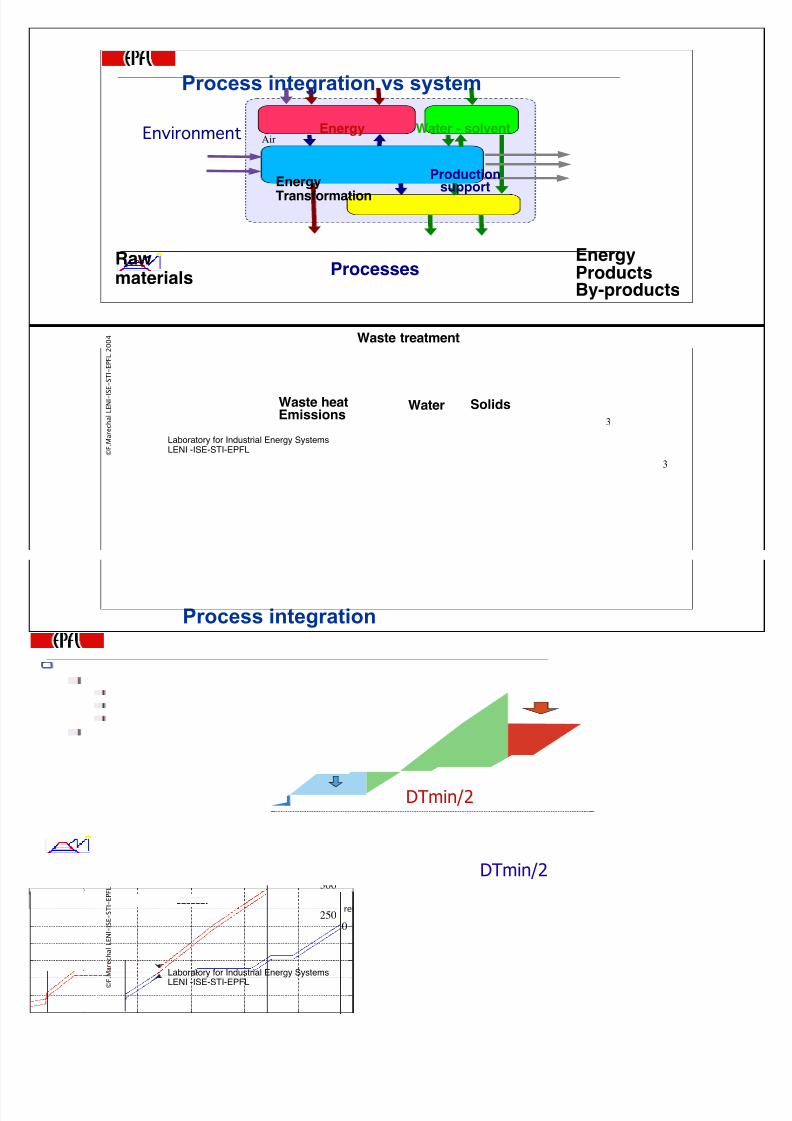
Process integration vs system

3

3

Energy

Transformation

Processes

Waste treatment

Productionsupport

Rawmaterials

EnergyProductsBy-products

Energy Water - solvent

Waste heatEmissions

Environment Air

Water Solids




Process integration

Hot & cold composite curves

Minimum energy requirementHot

Cold

Refrigeration

Heat recovery

4

REFRIGERATION

(EATRECOVERY

(OTUTILITY

COOLINGUTILITY

250

300

350

400

450

500

550

600

0 5000 10000 15000 20000 25000 30000

T ( K )

Q(kW)

Cold composite curveHot composite curve

K7

K7

K7

K7

$4MINDTmin/2

DTmin/2





E - S T I - E P F L 2 0 0 4

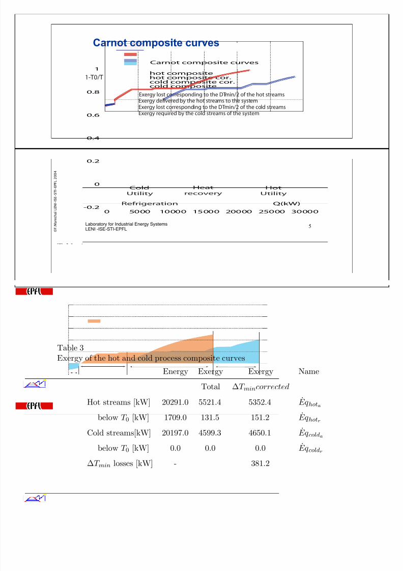
Carnot composite curves

5

(OT

5TILITY

#OLD

5TILITY

2EFRIGERATION

(EAT

RECOVERY

1K7

#ARNOTCOMPOSITECURVES

HOTCOMPOSITEHOTCOMPOSITECORCOLDCOMPOSITECORCOLDCOMPOSITE

44

%XERGYLOSTCORRESPONDINGTOTHE$4MINOFTHEHOTSTREAMS

%XERGYDELIVEREDBYTHEHOTSTREAMSTOTHESYSTEM

%XERGYREQUIREDBYTHECOLDSTREAMSOFTHESYSTEM%XERGYLOSTCORRESPONDINGTOTHE$4MINOFTHECOLDSTREAMS




6

Table 3Exergy of the hot and cold process composite curves

Energy Exergy Exergy Name

Total ∆T mincorrected

Hot streams [kW] 20291.0 5521.4 5352.4 Eq hota

below T 0 [kW] 1709.0 131.5 151.2 Eq hotr

Cold streams[kW] 20197.0 4599.3 4650.1 Eq colda

below T 0 [kW] 0.0 0.0 0.0 Eq coldr

∆T min losses [kW] - 381.2





E - S T I - E P F L 2 0 0 4

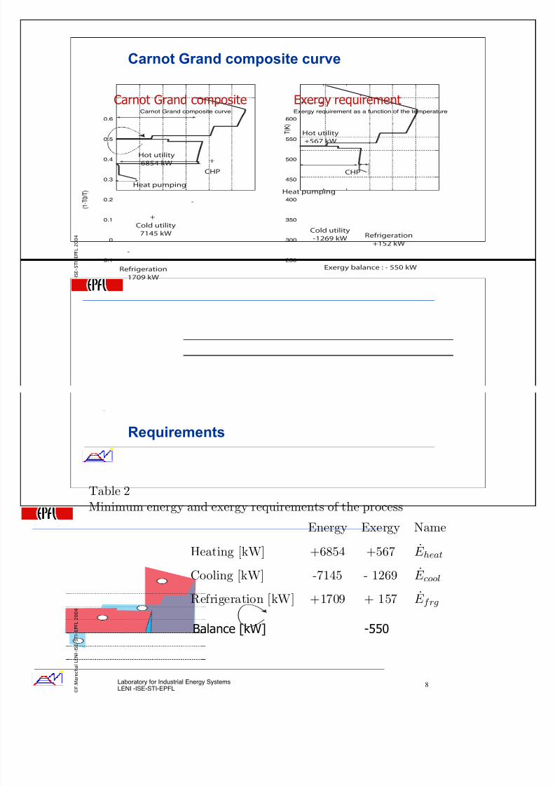
Carnot Grand composite curve

7

#(0

-0.2

-0.1

0

0.1

0.2

0.3

0.4

0.5

0.6

0 2000 4000 6000 8000 10000 12000

( 1 - T 0 / T )

Q(kW)

Carnot Grand composite curve

200

250

300

350

400

450

500

550

600

0 500 1000 1500 2000 2500 3000

T ( K )

Exergy (kW, T0 : 298.1K)

Exergy requirement as a function of the temperature

2EFRIGERATION

K7

#OLDUTILITY

K7 #OLDUTILITY

K7

2EFRIGERATION

K7

(EATPUMPING

%XERGYBALANCEK7

(EATPUMPING

#(0

(OTUTILITY

K7

(OTUTILITY

K7

Exergy requirementCarnot Grand composite




Requirements

8

Table 2Minimum energy and exergy requirements of the process

Energy Exergy Name

Heating [kW] +6854 +567 E heat

Cooling [kW] -7145 - 1269 E cool

Refrigeration [kW] +1709 + 157 E frg

Balance [kW] -550





E - S T I - E P F L 2 0 0 4

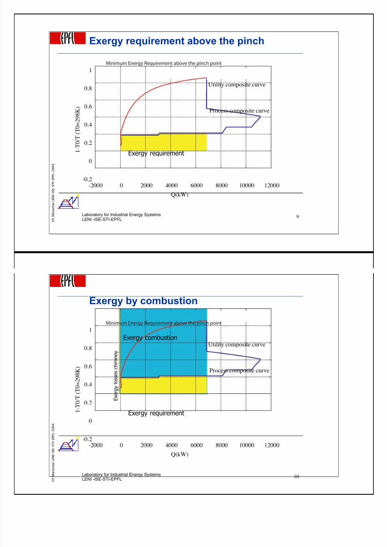
-0.2

0

0.2

0.4

0.6

0.8

1

-2000 0 2000 4000 6000 8000 10000 12000

1 - T 0 / T ( T 0 = 2 9 8 K )

Q(kW)

Process composite curve

Utility composite curve

-INIMUM%NERGY2EQUIREMENTABOVETHEPINCHPOINT

Exergy requirement

Exergy requirement above the pinch

9




Exergy by combustion

10

-0.2

0

0.2

0.4

0.6

0.8

1

-2000 0 2000 4000 6000 8000 10000 12000

1 - T 0 / T ( T 0 =

2 9 8 K )

Q(kW)




Exergy combustion

Exergy requirement

E x e r g y l o

s s e s c h i m n e y





E - S T I - E P F L 2 0 0 4

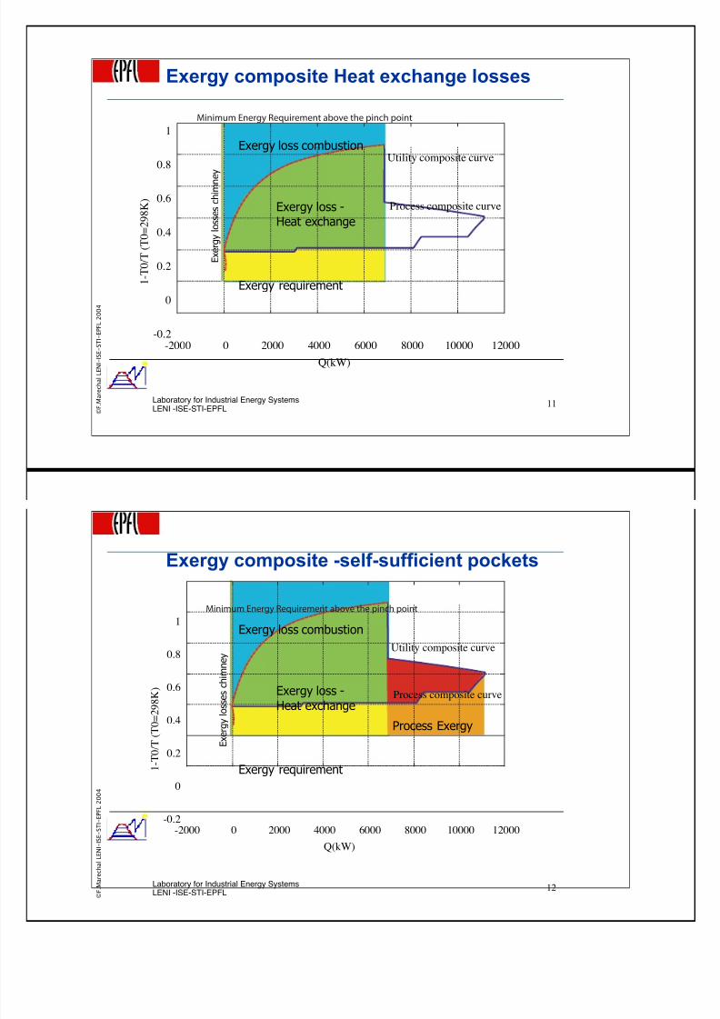
Exergy composite Heat exchange losses

11

-0.2

0

0.2

0.4

0.6

0.8

1

-2000 0 2000 4000 6000 8000 10000 12000

1 - T 0 / T ( T 0 = 2 9 8 K )

Q(kW)




Exergy loss -Heat exchange

Exergy requirement

Exergy loss combustion

E x e r g y l o s s e s c h i m n e

y




Exergy composite -self-sufficient pockets

12

-0.2

0

0.2

0.4

0.6

0.8

1

-2000 0 2000 4000 6000 8000 10000 12000

1 - T 0 / T ( T 0 = 2

9 8 K )

Q(kW)




Exergy loss -

Heat exchange

Exergy requirement

Exergy loss combustion

Process Exergy

E x e r g y l o

s s e s c h i m n e y





E - S T I - E P F L 2 0 0 4

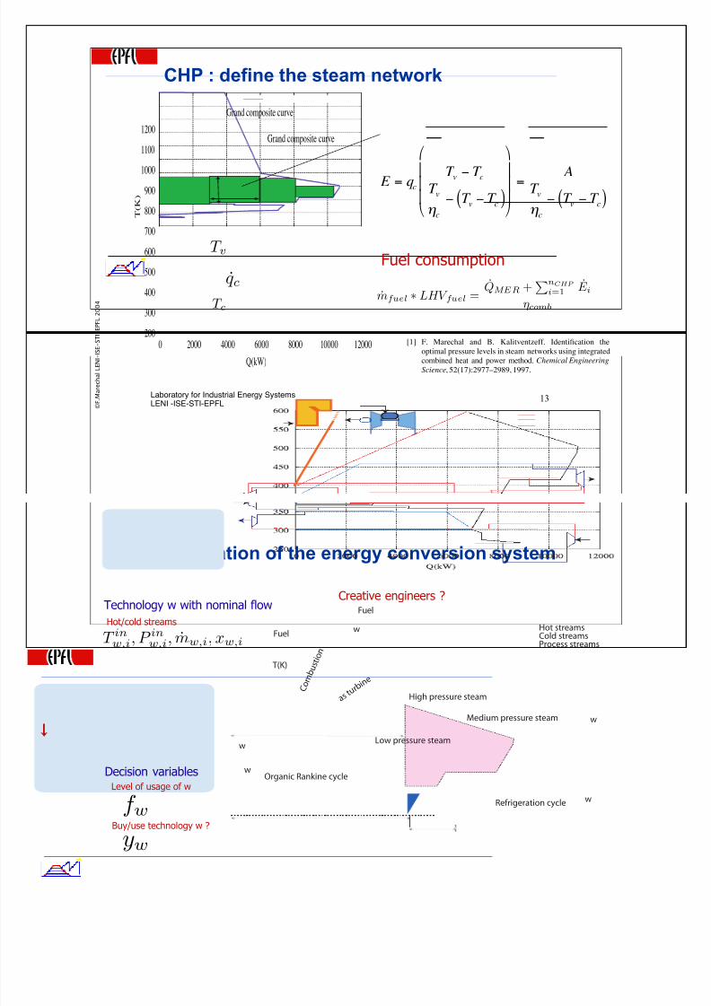
CHP : define the steam network

13

200

300

400

500

600

700

800

9001000

1100

1200

0 2000 4000 6000 8000 10000 12000

T ( K )

Q(kW)

Grand composite curve

Grand composite curve

˙ E = qc

T v " T cT v

#c

" T v " T

c( )

$

%

&

& &

'

(

)

) ) = AT v

#c

" T v " T

c( )

q c

T v

T c

[1]! F. " Marechal and B. " Kalitventzeff. Identification the

optimal pressure levels in steam networks using integratedcombined heat and power method. Chemical Engineering

Science, 52(17):2977–2989, 1997.

mfuel ∗ LHV fuel =QMER +

nCHP i=1 E i

ηcomb

Fuel consumption




Technology w with nominal flow

T outw,i , P outw,i , mw,i, xw,i

T inw,i, P inw,i, mw,i, xw,i

q w = mw,i(hinw,i − houtw,i)

Hot/cold streams

Mechanical power/electricity

Costs

C 1w, C 2w, CI 1w, CI 2w

ew

Integration of the energy conversion system

14

(OT 5TILITY K73ELF SUFFICIENT

0OCKET

#OLD UTILITY K7

2EFRIGERATION K7

HEATPUMPS

'

A S T U R B

I N E

(IGHPRESSURESTEAM

W

# O M B

U S T I O

N

W

W

W

-EDIUMPRESSURESTEAM

,OWPRESSURESTEAM

2EFRIGERATIONCYCLE

/RGANIC2ANKINECYCLE

(OTSTREAMS#OLDSTREAMS0ROCESSSTREAMS

4+

W

&UEL

&UEL

f w

yw

Level of usage of w

Buy/use technology w ?

Decision variables

Creative engineers ?





E - S T I - E P F L 2 0 0 4

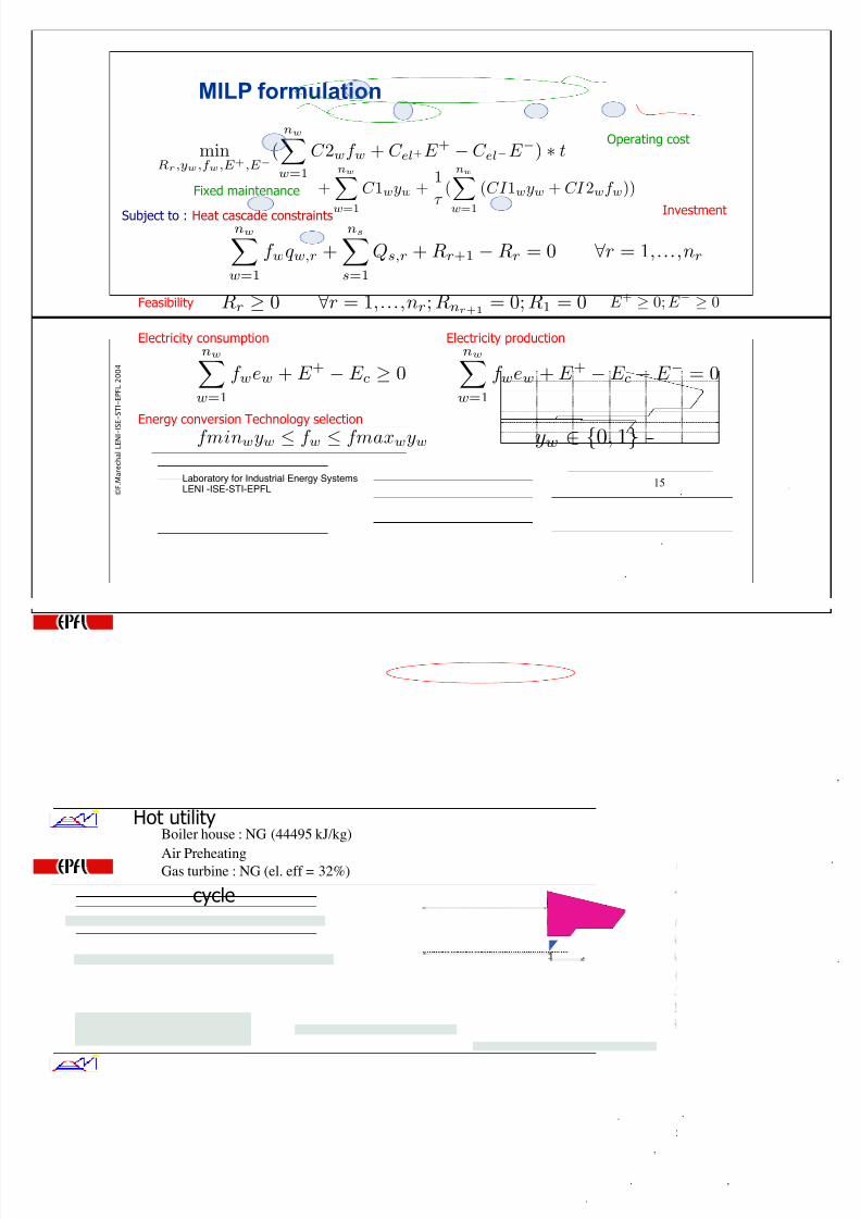
MILP formulation

15

minRr,yw,f w,E +,E −

(

nw

w=1

C 2wf w + C el+E +−C el−E

−) ∗ t

+

nw

w=1

C 1wyw +1

τ

(

nw

w=1

(CI 1wyw + CI 2wf w))

nw

w=1

f wq w,r +

ns

s=1

Qs,r + Rr+1 −Rr = 0 ∀ r = 1,...,nr

Rr ≥ 0 ∀r = 1,...,nr; Rnr+1= 0; R1 = 0

nw

w=1

f wew +E + − E c ≥ 0

nw

w=1

f wew +E + − E c − E − = 0

fminwyw ≤ f w ≤ fmaxwyw yw ∈ {0, 1}

E +≥ 0;E

−

≥ 0

Subject to : Heat cascade constraints

Electricity consumption Electricity production

Feasibility

Energy conversion Technology selection

Operating cost

Fixed maintenance

Investment




Application

16

Energy Exergy

Heating (kW) +6854 +567

Cooling (kW) -6948 - 1269

Refrigeration (kW) +1709 + 157

Maximum energy recovery

Hot Utility :6854 kWSelf sufficient"Pocket"

Ambient temperature

Cold utility :6948 kW

Refrigeration :1709 kW250

300

350

400

450

500

550

600

0 2000 4000 6000 8000 10000 12000

T ( K )

Q(kW)

.

.

.

.

.

.

.

.

.

,

.

,

.

:

Ref rigerant R717 Ammonia

Reference flowrate 0.1 kmol/s

Mechanical power 394 kW

P T in T out Q !Tmin/2

(bar) ( °K) ( °K) kW (°K)

Hot str. 12 340 304 2274 2

Cold str. 3 264 264 1880 2

,

.

. ,

:

:

,

.

.

.

.

:

Refrigeration: ,

Plow T low Phigh T high COP kWe

(bar ) ( °K) ( ba r) (K) -

Cycle 3 5 354 7.5 371 15 130

Cycle 2 6 361 10 384 12 323

Cycle 0 6 361 7.5 371 28 34

:

−

−

.

,.

.

:

,

.

Heat pumpsFluid R123

Header P T Comment

(bar) (K)

HP2 92 793 superheated

HP1 39 707 superheated

HPU 32 510 c ondensation

MPU 7.66 442 condensation

LPU 4.28 419 cond ensation

LPU2 2.59 402 condensation

LPU3 1.29 380 condensation

DEA 1.15 377 deaeration

Steam cycle

Boiler house : NG (44495 kJ/kg)

Air PreheatingGas turbine : NG (el. eff = 32%)

Hot utility





E - S T I - E P F L 2 0 0 4

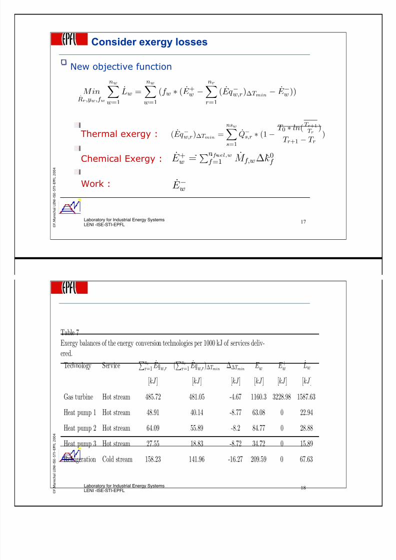
New objective function

Thermal exergy :

Chemical Exergy :

Work :

Consider exergy losses

17

MinRr,yw,f w

nw

w=1

Lw =

nw

w=1

(f w ∗ (E +w −

nr

r=1

(Eq −w,r)∆T min − E −w ))

(Eq −w,r)∆T min =

nsw

s=1

Q−s,r ∗ (1−T 0 ∗ ln(

T r+1T r

)

T r+1 − T r)

E +w =nfuel,w

f =1 M f,w∆k0f

E −w




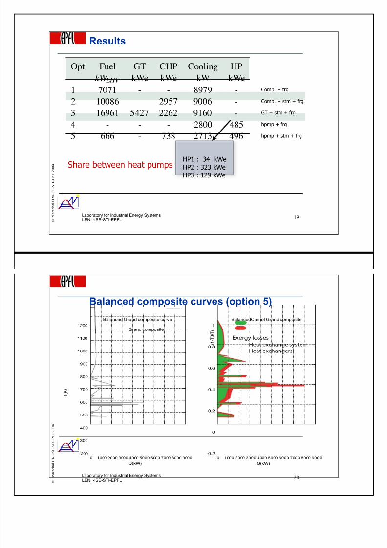
18

Table 7Exergy balances of the energy conversion technologies per 1000 kJ of services deliv-ered.

Technology Servicenr

r=1 Eq−

w,r (nr

r=1 Eq−

w,r)∆T min∆∆T min

E −w E +w Lw

[kJ ] [kJ ] [kJ ] [kJ ] [kJ ] [kJ ]

Gas turbine Hot stream 485.72 481.05 -4.67 1160.3 3228.98 1587.63

Heat pump 1 Hot stream 48.91 40.14 -8.77 63.08 0 22.94



Refrigeration Cold stream 158.23 141.96 -16.27 209.59 0 67.63





E - S T I - E P F L 2 0 0 4

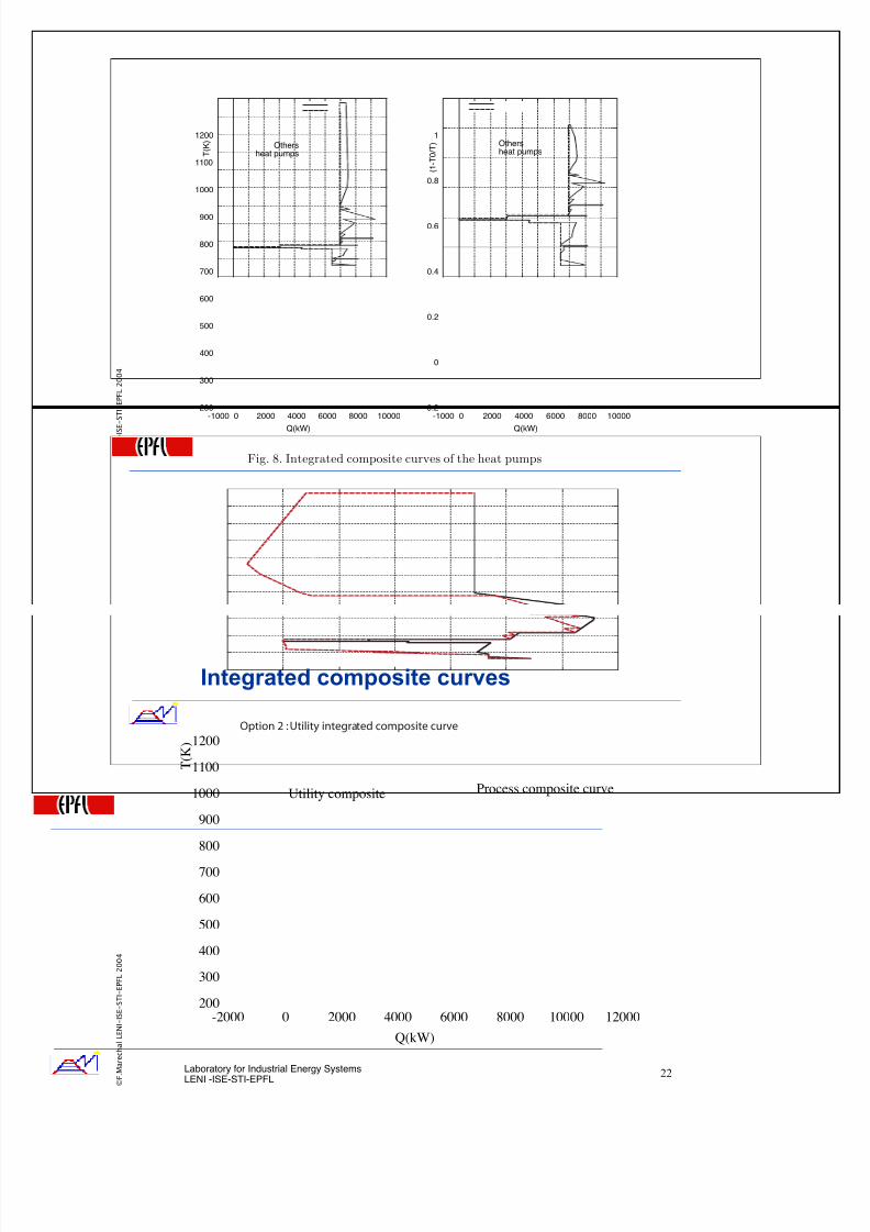
Results

19

Opt Fuel GT CHP Cooling HP

kW LHV kWe kWe kW kWe

1 7071 - - 8979 -

2 10086 2957 9006 -

3 16961 5427 2262 9160 -

4 - - - 2800 485

5 666 - 738 2713 496

Comb. + frg

Comb. + stm + frg

GT + stm + frg

hpmp + frg

hpmp + stm + frg

HP1 : 34 kWe

HP2 : 323 kWeHP3 : 129 kWe

Share between heat pumps




Balanced composite curves (option 5)

20

200

300

400

500

600

700

800

900

1000

1100

1200

0 1000 2000 3000 4000 5000 6000 7000 8000 9000

T ( K )

Q(kW)

Balanced Grand composite curve

Grand composite

-0.2

0

0.2

0.4

0.6

0.8

1

0 1000 2000 3000 4000 5000 6000 7000 8000 9000

( 1 - T 0 / T )

Q(kW)

BalancedCarnot Grand composite

(EATEXCHANGESYSTEM

(EATEXCHANGERS

%XERGYLOSSES





E - S T I - E P F L 2 0 0 4

200

300

400

500

600

700

800

900

1000

1100

1200

-1000 0 2000 4000 6000 8000 10000

T ( K )

Q(kW)

Othersheat pumps

-0.2

0

0.2

0.4

0.6

0.8

1

-1000 0 2000 4000 6000 8000 10000

( 1 - T 0 / T )

Q(kW)

Othersheat pumps

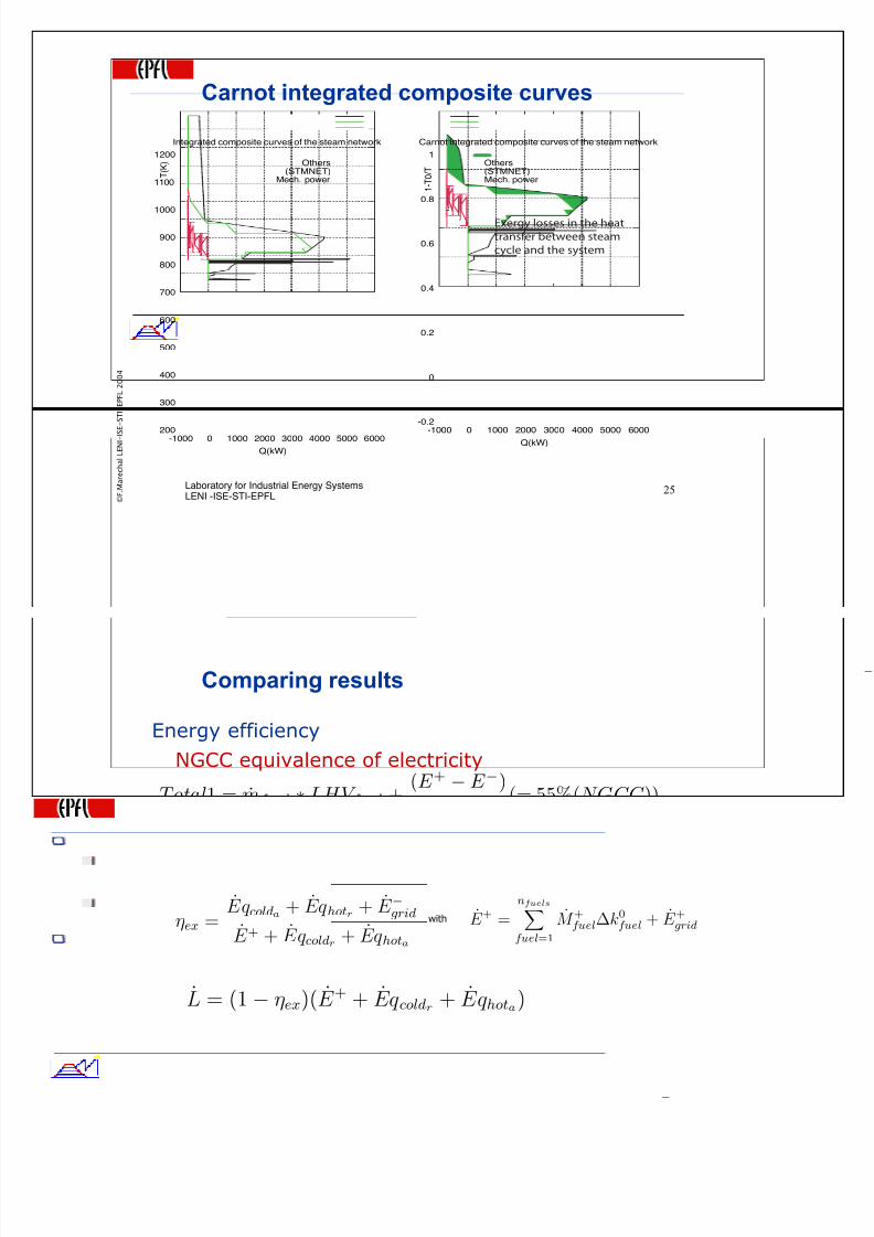
Fig. 8. Integrated composite curves of the heat pumps




Integrated composite curves

22

200

300

400

500

600

700

800

900

1000

1100

1200

-2000 0 2000 4000 6000 8000 10000 12000

T ( K )

Q(kW)

Process composite curveUtility composite

/PTION5TILITYINTEGRATEDCOMPOSITECURVE





E - S T I - E P F L 2 0 0 4

Integrated composite curve : steam network

23




Visualising the results : Carnot efficiency

24

-0.2

0

0.2

0.4

0.6

0.8

1

-2000 0 2000 4000 6000 8000 10000 12000

1 - T 0 / T

Q(kW)

Option 1 : Carnot composite curves

Process composite curveUtility composite curve

-0.2

0

0.2

0.4

0.6

0.8

1

-2000 0 2000 4000 6000 8000 10000 12000

1 - T 0 / T

Q(kW)

Option 5 : Carnot composite curves

Process composite curveUtility composite curve

Tricks for creative engineers : reduce the green area !





E - S T I - E P F L 2 0 0 4

Carnot integrated composite curves

25

200

300

400

500

600

700

800

900

1000

1100

1200

-1000 0 1000 2000 3000 4000 5000 6000

T ( K )

Q(kW)

Integrated composite curves of the steam network

Others(STMNET)

Mech. power

-0.2

0

0.2

0.4

0.6

0.8

1

-1000 0 1000 2000 3000 4000 5000 6000

1 - T 0 / T

Q(kW)

Carnot integrated composite curves of the steam network

Others(STMNET)Mech. power

%XERGYLOSSESINTHEHEAT

TRANSFERBETWEENSTEAM

CYCLEANDTHESYSTEM




Energy efficiency

NGCC equivalence of electricity

EU mix for electricity

Exergy efficiency

Comparing results

26

Total2 = mfuel ∗ LHV fuel +(E + −E

−)

ηel

(= 38%(EUmix))

Total1 = mfuel ∗ LHV fuel +(E + −E −)

ηel

(= 55%(NGCC ))

ηex =Eq colda + Eq hotr + E −grid

E + + Eq coldr + Eq hota

−

E + =nfuels

fuel=1

M +fuel∆k0

fuel + E +grid

−

with

L = (1− ηex)(E + + Eq coldr + Eq hota)





E - S T I - E P F L 2 0 0 4

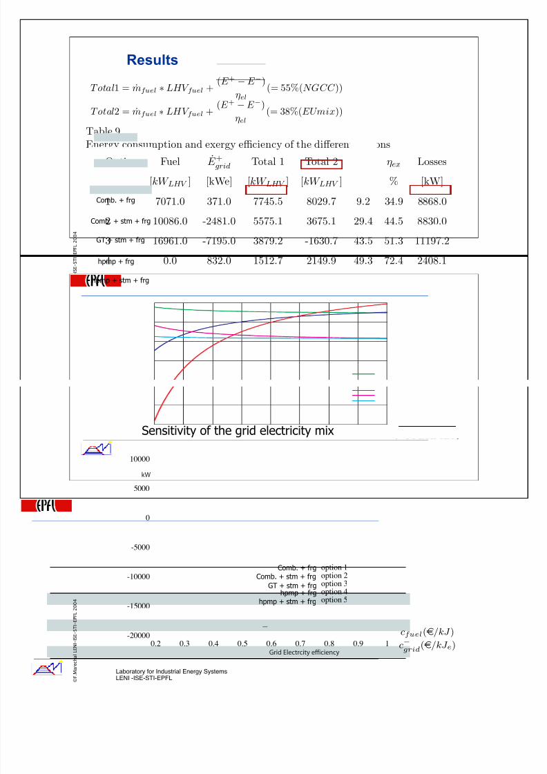
Table 9Energy consumption and exergy efficiency of the diff erent options

Option Fuel E +

gridTotal 1 Total 2 ηec ηex Losses

[kW LHV ] [kWe] [kW LHV ] [kW LHV ] % % [kW]

1 7071.0 371.0 7745.5 8029.7 9.2 34.9 8868.0

2 10086.0 -2481.0 5575.1 3675.1 29.4 44.5 8830.0

3 16961.0 -7195.0 3879.2 -1630.7 43.5 51.3 11197.2

4 0.0 832.0 1512.7 2149.9 49.3 72.4 2408.1

5 666.0 125.0 893.3 989.0 49.6 72.6 1831.6

Results

Comb. + frg

Comb. + stm + frg

GT + stm + frg

hpmp + frg

hpmp + stm + frg


−)

ηel(= 38%(EUmix))


−)

ηel

(= 55%(NGCC ))




-20000

-15000

-10000

-5000

0

5000

10000

0.2 0.3 0.4 0.5 0.6 0.7 0.8 0.9 1

option 1option 2option 3option 4option 5

'RID%LECTRCITYEFFICIENCY

K7

Sensitivity of the grid electricity mix

Comb. + frgComb. + stm + frg

GT + stm + frghpmp + frg

hpmp + stm + frg

−

cfuel(e/kJ )

c−grid

(e/kJ e)





E - S T I - E P F L 2 0 0 4

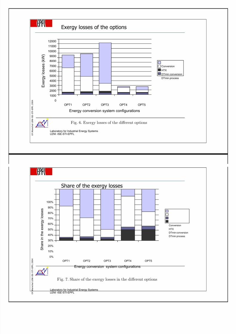
OPT1 OPT2 OPT3 OPT4 OPT5

0

1000

2000

3000

4000

5000

6000

7000

8000

9000

10000

11000

12000

Conversion

HTX

DTmin conversion

DTmin process

Energy conversion system configurations

E x e r g y l o s s e s ( k W

)

Fig. 6. Exergy losses of the diff erent options

Exergy losses of the options




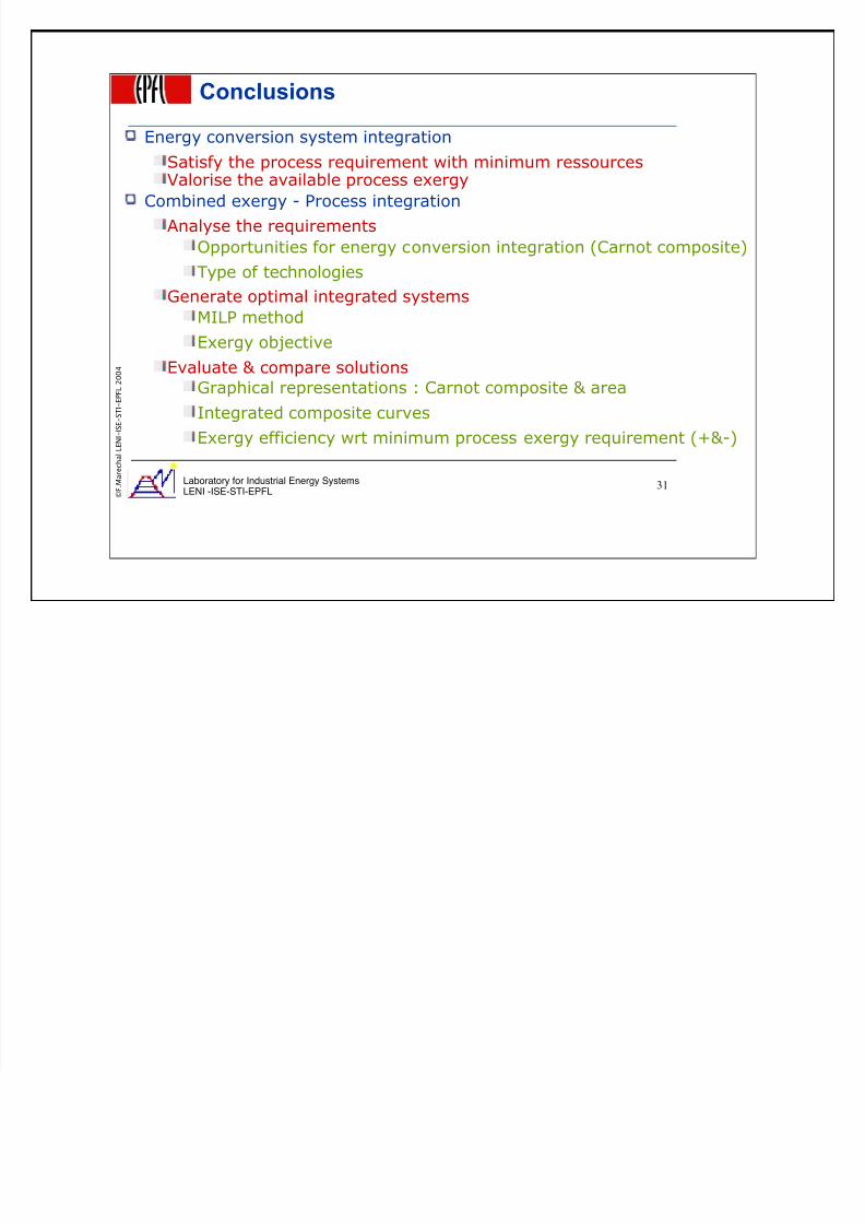
OPT1 OPT2 OPT3 OPT4 OPT5

0%

10%

20%

30%

40%

50%

60%

70%

80%

90%

100%

Conversion

HTX

DTmin conversionDTmin process

Energy conversion system configurations

S h a r e

i n

t h

e

e x e r g y

l o s s e s

Fig. 7. Share of the exergy losses in the diff erent options

Share of the exergy losses





E - S T I - E P F L 2 0 0 4

Conclusions

Energy conversion system integration

Satisfy the process requirement with minimum ressourcesValorise the available process exergy

Combined exergy - Process integration

Analyse the requirements

Opportunities for energy conversion integration (Carnot composite)

Type of technologies

Generate optimal integrated systems

MILP method

Exergy objective

Evaluate & compare solutions

Graphical representations : Carnot composite & area

Integrated composite curves

Exergy efficiency wrt minimum process exergy requirement (+&-)

31

Documents

Exergy Pinch