Exercise:

Training Simple MLP by Backpropagation.

Using Netlab.

Petr Posık

December 11, 2007

1 File list

This document is an explanation text to the following script:

• demoMLPKlin.m — script implementing the beckpropagation algortihmderived in Sec. 2. Uses data set tren.dat and m-file mlperc.m whichimplements the neural network.

• demoNetlabKlin.m — constructs the same neural network as the firstscript (see Sec. 3.1), this time using Netlab (which must be downloadedseparately). Uses data set tren.dat and helper function plotData.m.

• demoNetlabXOR.m — uses Netlab to construct the neural network for theXOR data set, see Sec. 3.2 (trenXORrect.dat contains rectangular XORpattern, trenXOR.dat contains rotated version). Uses helper functionplotData.m.

2 Backpropagation for simple MLP

Suppose we have a training set that exhibits the pattern shown in Fig. 2:The task is to create a simple neural network classifier that would be able

to discriminate between red crosses and blue circles.

2.1 Preliminary questions

2.1.1 Is one simple perceptron sufficient to classify the training points

precisely?

No. One perceptron creates only one linear decision boundary.

2.1.2 How many linear boundaries do we need here?

At least two.

1

0 0.1 0.2 0.3 0.4 0.5 0.6 0.7 0.8 0.9 10

0.1

0.2

0.3

0.4

0.5

0.6

0.7

0.8

0.9

1

Figure 1: The first training set.

2.1.3 What architecture of the network will be suitable?

Well, we need two linear decision boundaries, i.e. two neurons—variables x1

and x2 will be the inputs to both of them.OK, but this would give us a network that has two outputs. We need addi-

tional neuron to combine the outputs of the first two neurons into one output.

2.1.4 We need to tune the NN to the training set. What is actually

tuned?

The weights w.

2.2 Questions for our network

2.2.1 What does our network look like?

Our network is depicted in Fig. 2.The output nonlinear function g is the same for all the three neurons:

g(a) =1

1 + e−λa(1)

To reiterate, its derivative in point a can be computed as

g′(a) = λg(a)(1− g(a)) (2)

2

3

3

x1

x2

w11

w12 w13

w21

w22w23

w31

w32 w33

a1

a2

a3

z1

z2

z3 o

Figure 2: Our neural network.

2.2.2 How many weights have to be tuned in our network?

It seems that 6. For two inputs to neuron 1, two inputs to neuron 2, and 2inputs for neuron 3. Really?

Well, all the neurons should also have additional input that is connected tovalue 1 (do you remember the homogeneous coordinates?). That’s why we have3 inputs for each of the 3 neurons which gives 9 weights.

2.2.3 Given an input vector x, how do we compute the output of

our NN?

We use forward propagation. The weights related to neuron 1 form a vectorw1 = (w11, w12, w13). Simlarly we have vectors of weights for neurons 2 and 3:w2 = (w21, w22, w23) and w3 = (w31, w32, w33).

For a given vector x = (x1, x2), we create a vector x in homogeneous coor-dinates:

x = (x1, x2, 1). (3)

Then we can compute the weighted sums a1 and a2 for neurons 1 and 2:

a1 = wT1 x, (4)

a2 = wT2 x, (5)

and we can also compute the outputs z1 and z2 of neurons 1 and 2:

z1 = g(a1), (6)

z2 = g(a2). (7)

Then, we can construct the input vector for the third neuron as

xH = (z1, z2, 1) (8)

and pass it through the third neuron

a3 = wT3 xH , and (9)

z3 = o = g(a3). (10)

This way we have gained the values of all the zi in the whole network.

3

2.2.4 How do we compute the weights of the network?

We define the loss function (optimization criterion) E as

E =1

2

N∑

n=1

C∑

c=1

(ync − onc)2. (11)

i.e. as the sum of squares of errors of all outputs (c = 1, . . . , C) for all trainingexamples (n = 1, . . . , N). However we can consider only the error for onetraining example:

E =1

2

C∑

c=1

(yc − oc)2. (12)

And, since our network has only one output, the error is defined as

E =1

2(y − o)2. (13)

Since the output o is actually a function of weights o(w), we can optimize theerror function E by modifying the weights. We shall use the gradient descentmethod. The update rule of the gradient descent method is

w← w − η · grad(E(w)) (14)

2.2.5 How do we compute the gradient?

The gradient in point w can be computed by using the backprop. algorithm.In our case, the gradient can be written as a matrix (similarly as w):

grad(E(w)) =

∂E∂w11

∂E∂w12

∂E∂w13

∂E∂w21

∂E∂w22

∂E∂w23

∂E∂w31

∂E∂w32

∂E∂w33

(15)

From the derivation of the backpropagation algrotihm we know that theindividual derivatives can be computed as

∂E

∂wji

= δjzi, (16)

where δj is the error of the neuron on the output of the edge i → j, and zi isthe signal on the input of the edge i → j. Values of zis are known from theforward propagation phase, we need to compute the δjs.

Again, from the derivation of the backpropagation algorithm we know, thatfor the output layer we can write

δ3 = g′(a3)︸ ︷︷ ︸

λz3(1−z3)

∂E

∂o= λz3(1− z3) · (−1)(y − o) (17)

4

For the δjs in the hidden layer, we can write

δj = g′(aj)∑

k∈Dest(j)

wkjδk (18)

Consider neuron 1. The set of neurons which are fed with signal from neuron 1is Dest(1) = 3, so that the sum will have only one element:

δ1 = g′(a1)∑

k∈Dest(1)

wk1δk = (19)

= λz1(1− z1)w31δ3 (20)

Similarly, for the neuron 2 we can write

δ2 = λz2(1− z2)w32δ3 (21)

That completes the backpropagation algorithm for our particular network.We know the zis from the forward propagation, we have computed the δjsusing the backpropagation algorithm, we can thus compute the gradient of theerror function grad(E(w)) and make the gradient descent step w ← w − η ·

grad(E(w)).

2.2.6 How can that be written in MATLAB?

The following code is the MATLAB implementation of our derived procedure.The only difference is that we have derived the on-line version, the code is forbatch algorithm.

function err = train()

% W - [3 x 3] matrix of NN weights

% x - [nin x 2] matrix of coordinates x1 and x2

% y - [nin x 1] matrix of target values (1 or 0)

% Propagate training points through network

nin = size(x,1);

data = [x ones(nin ,1)];

z1 = perc(W(1,:), data);

z2 = perc(W(2,:), data);

data2 = [z1 z2 ones(nin ,1)];

z3 = perc(W(3,:), data2);

% Compute average error for 1 point

err = 0.5 * sum((y-z3) .^ 2) / nin;

% Delta in output layer , neuron 3

delta3 = lambda * z3 .* (1-z3) .* -(y-z3);

% Propagate errors back to hidden layer , neurons 1 and 2

5

delta1 = lambda * z1 .* (1-z1) .* delta3 * W(3,1);

delta2 = lambda * z2 .* (1-z2) .* delta3 * W(3,2);

% Compute the derivatives

dEdW1 = delta1 ’ * data;

dEdW2 = delta2 ’ * data;

dEdW3 = delta3 ’ * data2;

% Compile the gradient of the weight matrix

nablaEw = [dEdW1; dEdW2; dEdW3 ];

% Adapt the weights using the gradient descent rule

W = W - eta * nablaEw;

% Apply decay factor

eta = eta*quo;

end

2.2.7 How can we interpret the weights after learning?

After repeatedly running the training algorithm for e.g. 1000 iterations, wehopefully get near-optimal weights. The meaning of individual parts of ourtrained NN can be seen in Fig. 3

3 Using Netlab

Netlab1 is a set of MATLAB functions that allows us to create simple neuralnetworks (among other things). It was created by Ian Nabney and ChristopherBishop who is the author of the very popular book Neural Networks for PatternRecognition.

3.1 Netlab and our first data set

3.1.1 Crucial functions of Netlab

First, we apply the Netlab to solve the same problem as in previous section.The important part of the script can be seen here:

%% Suppose:

% x - [ntr x 2] input part of training vectors

% y - [ntr x 1] output part of training vectors

% xt - [ntst x 2] input part of testing vectors

% yt - [ntst x 1] output part of testing vectors

1Download at http://www.ncrg.aston.ac.uk/netlab/.

6

0 0.1 0.2 0.3 0.4 0.5 0.6 0.7 0.8 0.9 10

0.1

0.2

0.3

0.4

0.5

0.6

0.7

0.8

0.9

1

Figure 3: The meaning of the elements in the net. Line — is a set of pointsfor which a1(x) = 0, line — is a set of points for which a1(x) = 1, line --- is aset of points for which a2(x) = 0, line --- is a set of points for which a2(x) = 1,and line — is the decision boundary of the whole network, i.e. set of points forwhich z3(x) = 0.5.

%% Create network structure

% 2 inputs , 2 neurons in hidden layer , 1 output.

% The nonlinear function for the output neuron is ’logistic ’.

% The nonlinear funtions for the neurons in hidden layer is

% hardwired and is hyperbolic tangent.

net = mlp(2,2,1,’logistic ’);

%% Set the options for optimization

options = zeros (1 ,18);

options (1) = 1; % This provides display of error values.

%% Optimize the network weights

% Train the network in structure ’net ’ to correctly classify

% input vectors x to outputs y using ’scg ’ (scaled conjugate

% gradients ).

[net , options] = netopt(net , options , x, y, ’scg’);

%% Compute the predictions of the trained network

% for the testing data

ypred = mlpfwd(net , xt);

7

% Compute errors on testing data

errors = yt - ypred;

As can be seen, for our purposes (multilayer perceptron) we need only 3functions of Netlab:

• net = mlp(nin, nhid, nout, func) which creates a data structure hold-ing the NN with nin inputs, nhid neurons in hidden layer, and nout out-puts. The nonliner function of output neurons is set to func. Furtherinfo: help mlp.

• net = netopt(net, options, x, y, ’scg’) which optimizes the NNweights (hidden in structure net that was created by function mlp) so thatthe NN will have the least possible error when classifing the training inputsx into training outputs y. It can use several optimization algorithms, oneof them is scaled conjugate gradients, i.e. scg. Further info: help netopt.

• ypred = mlpfwd(net, xt) which provides the predictions that the net

gives us when new data points xt are presented to our NN. Further info:help mlpfwd.

3.1.2 Netlab results on our first data set

If we train the same network on the same data as in previous section, we shallexpect very similar results. The difference is that (1) the nonlinear functionsin hidden layer are not logistic, but hyperbolic tangent, and (2) we do notuse gradient descent to optimize the weights, but rather the method of scaledconjugated gradients. The results of training can be seen in Fig. 4.

0 0.1 0.2 0.3 0.4 0.5 0.6 0.7 0.8 0.9 10

0.1

0.2

0.3

0.4

0.5

0.6

0.7

0.8

0.9

1

0 0.1 0.2 0.3 0.4 0.5 0.6 0.7 0.8 0.9 1

0

0.1

0.2

0.3

0.4

0.5

0.6

0.7

0.8

0.9

1

0

0.5

1

Figure 4: Results for the network from Fig. 2. Left: the decision boundary,right: the discrimination function.

3.2 Netlab and the XOR problem

Consider the pattern of training data points depicted in Fig. 5.

8

0 0.1 0.2 0.3 0.4 0.5 0.6 0.7 0.8 0.9 10

0.1

0.2

0.3

0.4

0.5

0.6

0.7

0.8

0.9

1

Figure 5: Training data forming the XOR pattern.

Similarly to our first data set, the two classes are not linearly separable. Itseems reasonable to use our 2-2-1 network for this data set as well.

3.2.1 Locally optimal solution

In Fig. 6, we can see one possible solution where the NN tries to separate onecorner of the training data from the rest of the patterns.

It can be seen that such a network makes pretty large error (see the imagetitle). However, there exists another solution of this problem which is very hardto obtain if the NN already encodes the decision boundary from Fig. 6, i.e. whenthe NN is in local optimum.

3.2.2 Globally optimal solution

A better solution is depicted in Fig. 7. The title of the left picture clearly showsthat the solution is better (makes lower error with respect to the given dataset).

Looking at Fig. 7, one can ask where did the second decision boundary comefrom. The same picture in somewhat larger scale reveals that there is no secondboundary, they are just 2 parts of 1 boundary, see Fig. 8.

3.2.3 More complex network

The first and the second datasets were similar in the respect that they are notlinearly separable. However, they are different in the aspect that the first data

9

0 0.1 0.2 0.3 0.4 0.5 0.6 0.7 0.8 0.9 10

0.1

0.2

0.3

0.4

0.5

0.6

0.7

0.8

0.9

1Approx. training error: 165.64

0 0.1 0.2 0.3 0.4 0.5 0.6 0.7 0.8 0.9 1

0

0.1

0.2

0.3

0.4

0.5

0.6

0.7

0.8

0.9

1

0

0.5

1

Figure 6: Locally optimal solution of the network from Fig. 2 applied to theXOR pattern. Left: the decision boundary, right: the discrimination function.

0 0.1 0.2 0.3 0.4 0.5 0.6 0.7 0.8 0.9 10

0.1

0.2

0.3

0.4

0.5

0.6

0.7

0.8

0.9

1Approx. training error: 96.81

0 0.1 0.2 0.3 0.4 0.5 0.6 0.7 0.8 0.9 1

0

0.1

0.2

0.3

0.4

0.5

0.6

0.7

0.8

0.9

1

0

0.5

1

Figure 7: Globally optimal solution of the network from Fig. 2 applied to theXOR pattern. Left: the decision boundary, right: the discrimination function.

set is separable by 1 decision boundary, the XOR pattern is not.The next step is to add 1 neuron to the hidden layer, which gives a 2-3-1

network. In that case the solution can look like that depicted in Fig. 9. Theresult seems to be almost perfect solution! All training points are classifiedcorrectly, the decision boundaries look like those that would be drawn by ahuman.

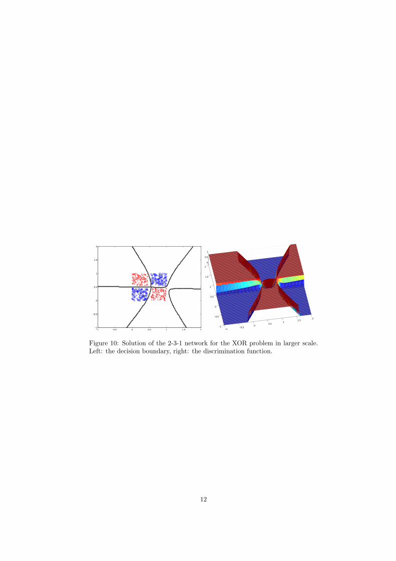
However, if you look at the solution in larger scale (see Fig. 10), you cansee that the boundaries are more ‘wild’ than expected. Moreover, although thelower right corner of the training data points is full of red crosses, the neuralnetwork produces there another decision boundary and creates there an areathat is classified as blue circles! Without any support in the training data!

This phenomenon can be observed in all types of machine learning models.A particular model has its own particular structural constraints that it imposeson the final form of the classifier. Only at the area that is covered by the training

10

−6 −4 −2 0 2 4 6

−6

−4

−2

0

2

4

6

−8 −6 −4 −2 0 2 4 6 8

−8

−6

−4

−2

0

2

4

6

8

0

0.5

1

Figure 8: Globally optimal solution of the network in larger scale. Left: thedecision boundary, right: the discrimination function.

0 0.1 0.2 0.3 0.4 0.5 0.6 0.7 0.8 0.9 10

0.1

0.2

0.3

0.4

0.5

0.6

0.7

0.8

0.9

1

0 0.1 0.2 0.3 0.4 0.5 0.6 0.7 0.8 0.9 1

0

0.1

0.2

0.3

0.4

0.5

0.6

0.7

0.8

0.9

1

0

0.5

1

Figure 9: Solution of the 2-3-1 network for the XOR problem. Left: the decisionboundary, right: the discrimination function.

data set, the predictions of the model can be influenced in a systematic way;in areas beyond the training set, each model extrapolates the values in its ownway—similarly as would be done e.g. by 2nd and 3rd order polynomials whenmodeling one-dimensional function.

11

−1 −0.5 0 0.5 1 1.5 2−1

−0.5

0

0.5

1

1.5

2

−1−0.5

00.5

11.5

2

−1

−0.5

0

0.5

1

1.5

2

0

0.5

1

Figure 10: Solution of the 2-3-1 network for the XOR problem in larger scale.Left: the decision boundary, right: the discrimination function.

12