Exercise

Numerical Analysis of Differential Equations

Fakultat fur Mathematik und InformatikTU Bergakademie Freiberg

Dr. M. Helm / Dipl.-Math. St. Pacholak

August 13, 2015

Contents

1 Initial Value Problems - Repetition 31.1 Comprehension Questions . . . . . . . . . . . . . . . . . . . . . . . . . . . 31.2 Mixing Tank . . . . . . . . . . . . . . . . . . . . . . . . . . . . . . . . . . . 41.3 Interconnected Tanks . . . . . . . . . . . . . . . . . . . . . . . . . . . . . . 51.4 Even more Tanks . . . . . . . . . . . . . . . . . . . . . . . . . . . . . . . . 61.5 Higher Order IVP . . . . . . . . . . . . . . . . . . . . . . . . . . . . . . . . 7

2 Initial Value Problems - Single-step Methods 82.1 Comprehension Questions . . . . . . . . . . . . . . . . . . . . . . . . . . . 82.2 EULER Methods . . . . . . . . . . . . . . . . . . . . . . . . . . . . . . . . 92.3 BUTCHER Arrays . . . . . . . . . . . . . . . . . . . . . . . . . . . . . . . 102.4 RUNGE-KUTTA Method . . . . . . . . . . . . . . . . . . . . . . . . . . . 112.5 Consistency . . . . . . . . . . . . . . . . . . . . . . . . . . . . . . . . . . . 122.6 Self study . . . . . . . . . . . . . . . . . . . . . . . . . . . . . . . . . . . . 13

3 Initial Value Problems - Multi-step Methods 143.1 Comprehension Questions . . . . . . . . . . . . . . . . . . . . . . . . . . . 143.2 Characteristic Polynoms . . . . . . . . . . . . . . . . . . . . . . . . . . . . 153.3 Order of Concistency . . . . . . . . . . . . . . . . . . . . . . . . . . . . . . 163.4 Concistency, Zero-Stability & Convergence . . . . . . . . . . . . . . . . . . 17

4 Initial Value Problems - MATLAB Training 184.1 Figures und Functions . . . . . . . . . . . . . . . . . . . . . . . . . . . . . 184.2 Subplots and Function Handles . . . . . . . . . . . . . . . . . . . . . . . . 19

5 Boundary Value Problems - Elliptic BVP 205.1 Comprehension Questions . . . . . . . . . . . . . . . . . . . . . . . . . . . 205.2 DIRICHLET Boundaries . . . . . . . . . . . . . . . . . . . . . . . . . . . . 215.3 Von NEUMANN Boundaries . . . . . . . . . . . . . . . . . . . . . . . . . . 225.4 Universal Grid Size . . . . . . . . . . . . . . . . . . . . . . . . . . . . . . . 235.5 DIRICHLET & von NEUMANN Boundaries . . . . . . . . . . . . . . . . . 245.6 Self Study . . . . . . . . . . . . . . . . . . . . . . . . . . . . . . . . . . . . 25

1

6 Boundary Value Problems - 1D & 2D 266.1 Square Grid Cells . . . . . . . . . . . . . . . . . . . . . . . . . . . . . . . . 266.2 Rectangular Grid Cells . . . . . . . . . . . . . . . . . . . . . . . . . . . . . 276.3 Discretization in Space and Time . . . . . . . . . . . . . . . . . . . . . . . 28

7 Assignment - Restricted 3-Body Problem 29

2

1 Initial Value Problems - Repetition

1.1 Comprehension Questions

I) The initial value problem y′(x) = f(x, y(x)) with y(a) = ya has a uniquesolution on [a,b], if:

A © © © f is continuous.B © © © f is continuous and Lipschitz continous in its second argument.C © © © f is differentiable.D © © © f is Lipschitz continous in its first argument.

II) Which of the following are NOT first order initial value problems?

A © © © dydx

= 2(x+ y) , y(0) = y0B © © © y′′ − 2y′ + y = tet − t , y(0) = 0C © © © y′ = 1

2y2 , y(1) = 1

D © © ©(y′1(t)y′2(t)

)=(

3 00 −2

)(y1(t)y2(t)

), y(

00

)=(

47

)

III) Which of the following statements are correct?

A © © © y′ =(

3 00 −2

)has the Eigenvalues λ1 = 3 and λ2 = −2.

B © © © The initial value problem dQdt

= r4 −

r100Q with Q(0) = Q0

has no solution in [0, te].C © © © dQ

dt= r

4 −r

100Q describes a predator-prey-interaction.

3

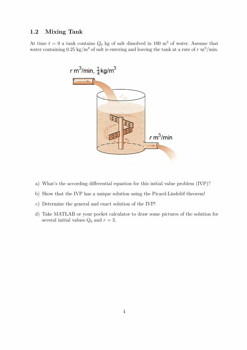
1.2 Mixing Tank

At time t = 0 a tank contains Q0 kg of salt dissolved in 100 m3 of water. Assume thatwater containing 0.25 kg/m3 of salt is entering and leaving the tank at a rate of r m3/min.

a) What’s the according differential equation for this initial value problem (IVP)?

b) Show that the IVP has a unique solution using the Picard-Lindelof theorem!

c) Determine the general and exact solution of the IVP!

d) Take MATLAB or your pocket calculator to draw some pictures of the solution forseveral initial values Q0 and r = 3.

4

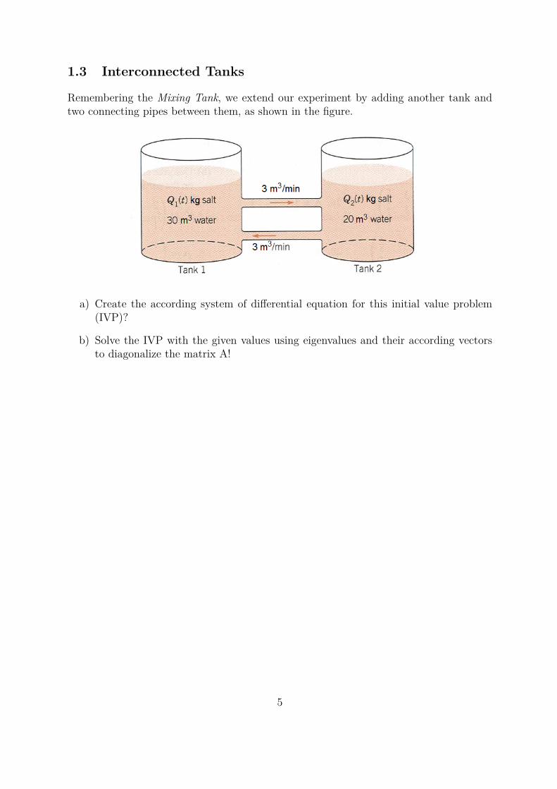
1.3 Interconnected Tanks

Remembering the Mixing Tank, we extend our experiment by adding another tank andtwo connecting pipes between them, as shown in the figure.

a) Create the according system of differential equation for this initial value problem(IVP)?

b) Solve the IVP with the given values using eigenvalues and their according vectorsto diagonalize the matrix A!

5

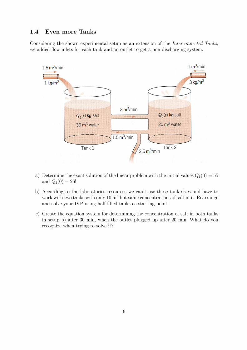
1.4 Even more Tanks

Considering the shown experimental setup as an extension of the Interconnected Tanks,we added flow inlets for each tank and an outlet to get a non discharging system.

a) Determine the exact solution of the linear problem with the initial values Q1(0) = 55and Q2(0) = 26!

b) According to the laboratories resources we can’t use these tank sizes and have towork with two tanks with only 10 m3 but same concentrations of salt in it. Rearrangeand solve your IVP using half filled tanks as starting point!

c) Create the equation system for determining the concentration of salt in both tanksin setup b) after 30 min, when the outlet plugged up after 20 min. What do yourecognize when trying to solve it?

6

1.5 Higher Order IVP

Rewrite the following higher order initial value problems from science and technicalapplication as first order systems!

a) y′′ − 2y′ + y = tet − t 0 ≤ t ≤ 1 y(0) = 0, y′(0) = 0

b) y′′′ = 12y

2 t ≥ 1 y(1) = 1, y′(1) = −1, y′′(1) = 2

c) t2y′′(t)− 2ty′(t) + 2y(t) = t3 ln t t ≥ 1 y(1) = 1, y′(1) = 0

7

2 Initial Value Problems - Single-step Methods

2.1 Comprehension Questions

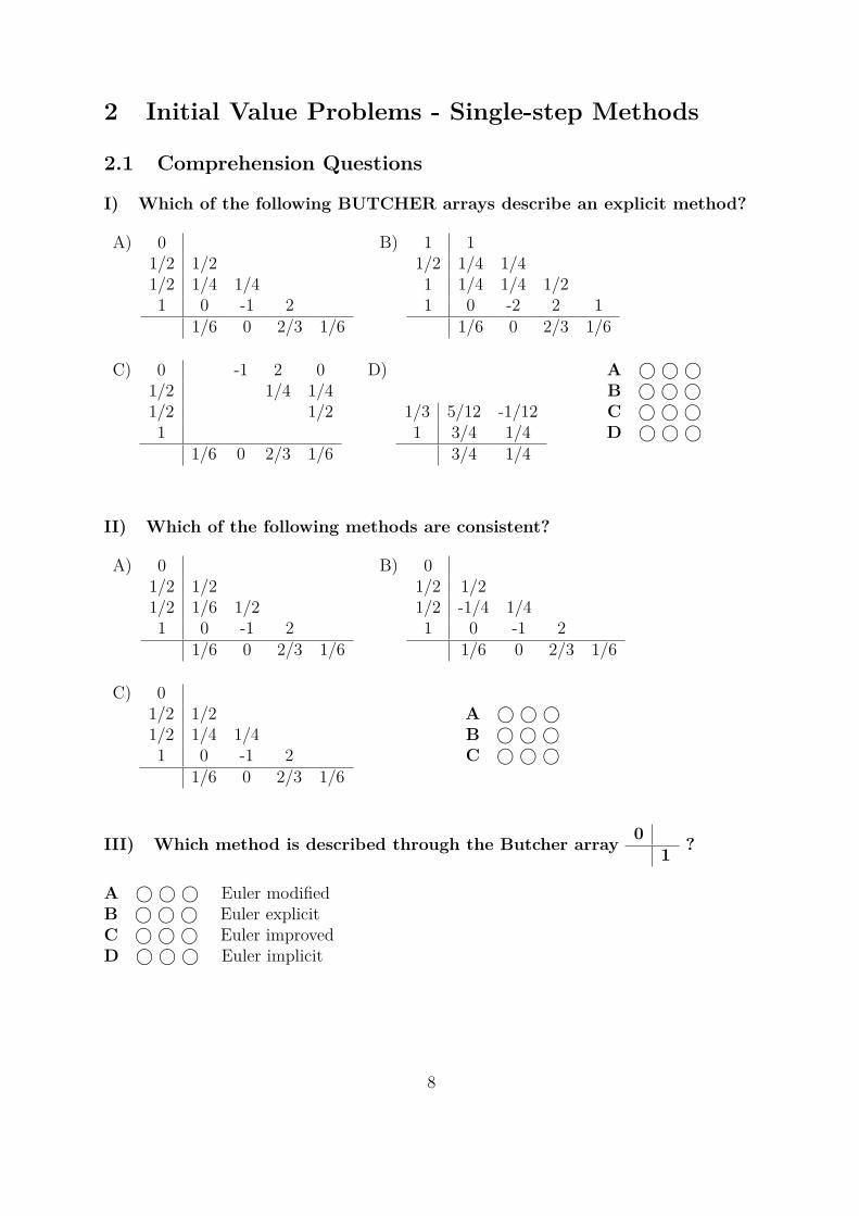
I) Which of the following BUTCHER arrays describe an explicit method?

A) 0 B) 1 11/2 1/2 1/2 1/4 1/41/2 1/4 1/4 1 1/4 1/4 1/21 0 -1 2 1 0 -2 2 1

1/6 0 2/3 1/6 1/6 0 2/3 1/6

C) 0 -1 2 0 D) A © © ©1/2 1/4 1/4 B © © ©1/2 1/2 1/3 5/12 -1/12 C © © ©1 1 3/4 1/4 D © © ©

1/6 0 2/3 1/6 3/4 1/4

II) Which of the following methods are consistent?

A) 0 B) 01/2 1/2 1/2 1/21/2 1/6 1/2 1/2 -1/4 1/41 0 -1 2 1 0 -1 2

1/6 0 2/3 1/6 1/6 0 2/3 1/6

C) 01/2 1/2 A © © ©1/2 1/4 1/4 B © © ©1 0 -1 2 C © © ©

1/6 0 2/3 1/6

III) Which method is described through the Butcher array 01 ?

A © © © Euler modifiedB © © © Euler explicitC © © © Euler improvedD © © © Euler implicit

8

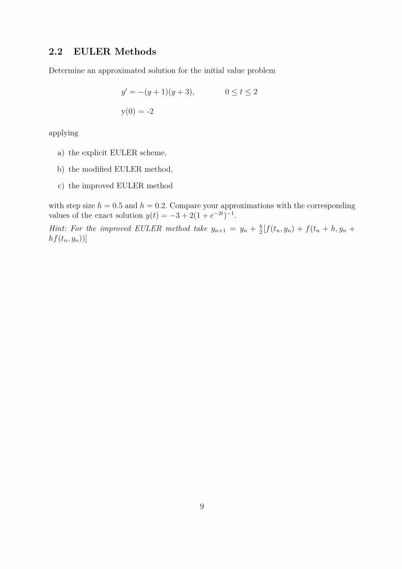
2.2 EULER Methods

Determine an approximated solution for the initial value problem

y′ = −(y + 1)(y + 3), 0 ≤ t ≤ 2

y(0) = -2

applying

a) the explicit EULER scheme,

b) the modified EULER method,

c) the improved EULER method

with step size h = 0.5 and h = 0.2. Compare your approximations with the correspondingvalues of the exact solution y(t) = −3 + 2(1 + e−2t)−1.Hint: For the improved EULER method take yn+1 = yn + h

2 [f(tn, yn) + f(tn + h, yn +hf(tn, yn))]

9

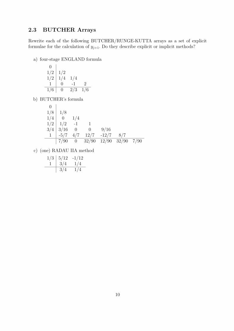
2.3 BUTCHER Arrays

Rewrite each of the following BUTCHER/RUNGE-KUTTA arrays as a set of explicitformulae for the calculation of yj+1. Do they describe explicit or implicit methods?

a) four-stage ENGLAND formula0

1/2 1/21/2 1/4 1/41 0 -1 2

1/6 0 2/3 1/6

b) BUTCHER’s formula0

1/8 1/81/4 0 1/41/2 1/2 -1 13/4 3/16 0 0 9/161 -5/7 4/7 12/7 -12/7 8/7

7/90 0 32/90 12/90 32/90 7/90

c) (one) RADAU IIA method1/3 5/12 -1/121 3/4 1/4

3/4 1/4

10

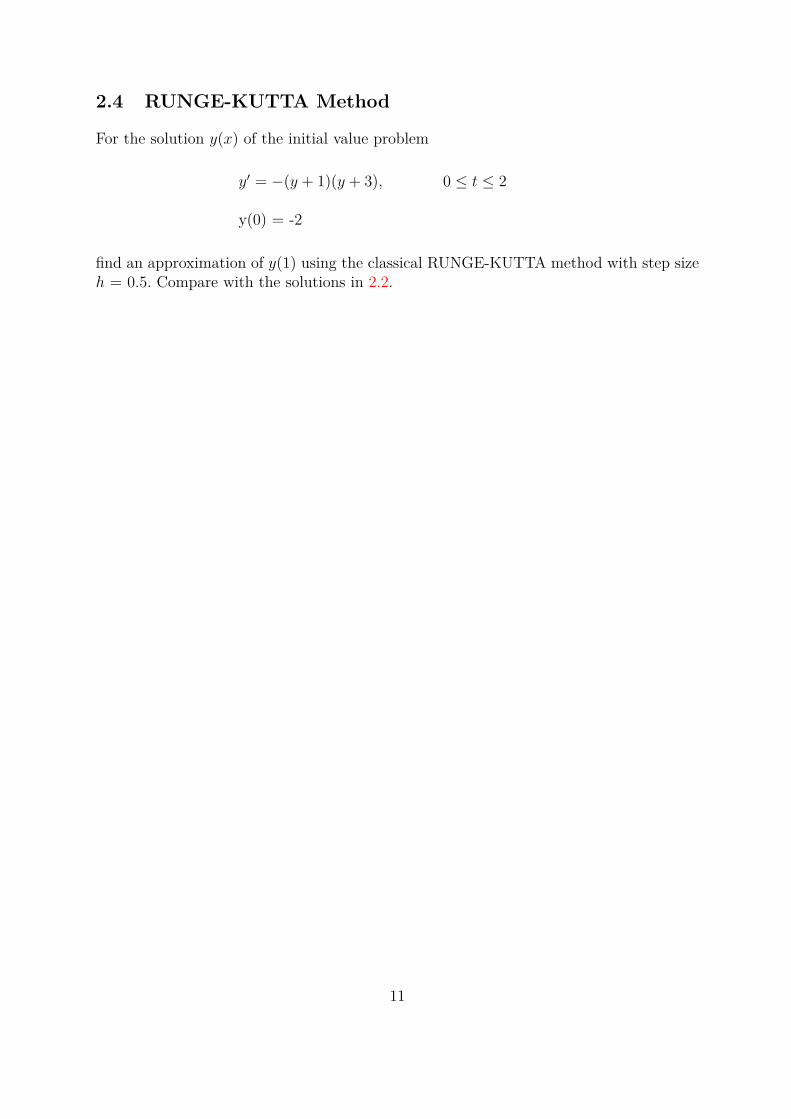
2.4 RUNGE-KUTTA Method

For the solution y(x) of the initial value problem

y′ = −(y + 1)(y + 3), 0 ≤ t ≤ 2

y(0) = -2

find an approximation of y(1) using the classical RUNGE-KUTTA method with step sizeh = 0.5. Compare with the solutions in 2.2.

11

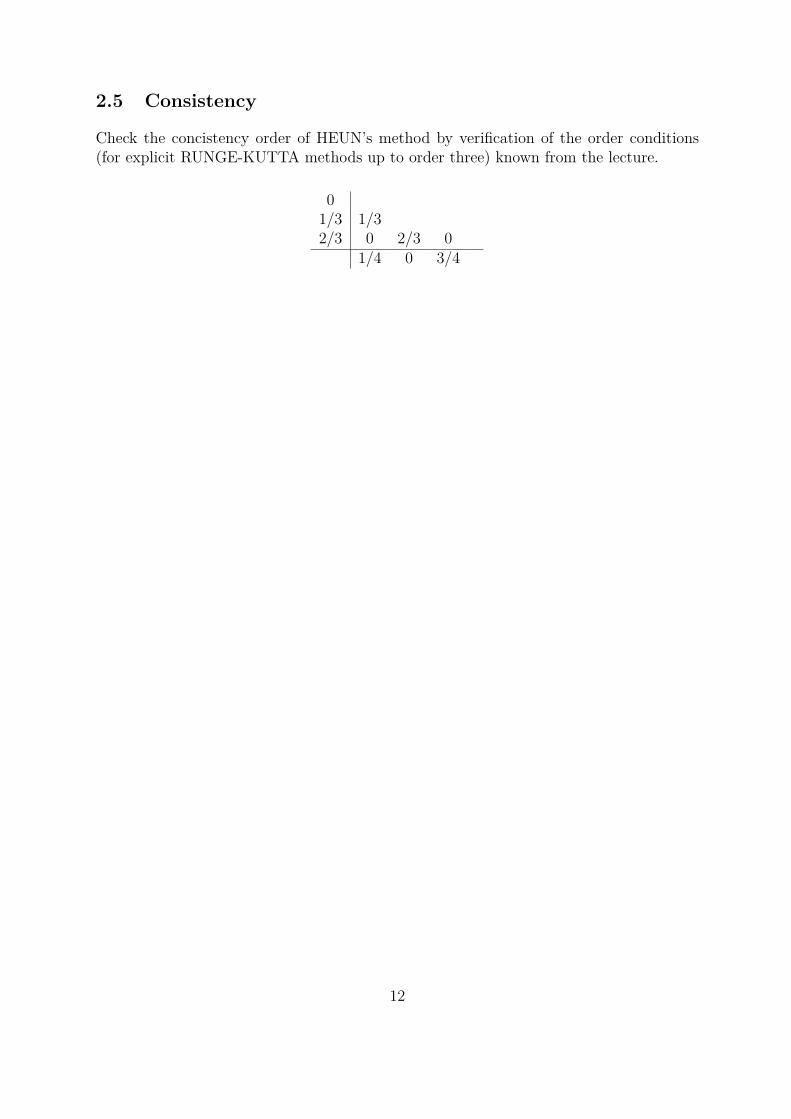
2.5 Consistency

Check the concistency order of HEUN’s method by verification of the order conditions(for explicit RUNGE-KUTTA methods up to order three) known from the lecture.

01/3 1/32/3 0 2/3 0

1/4 0 3/4

12

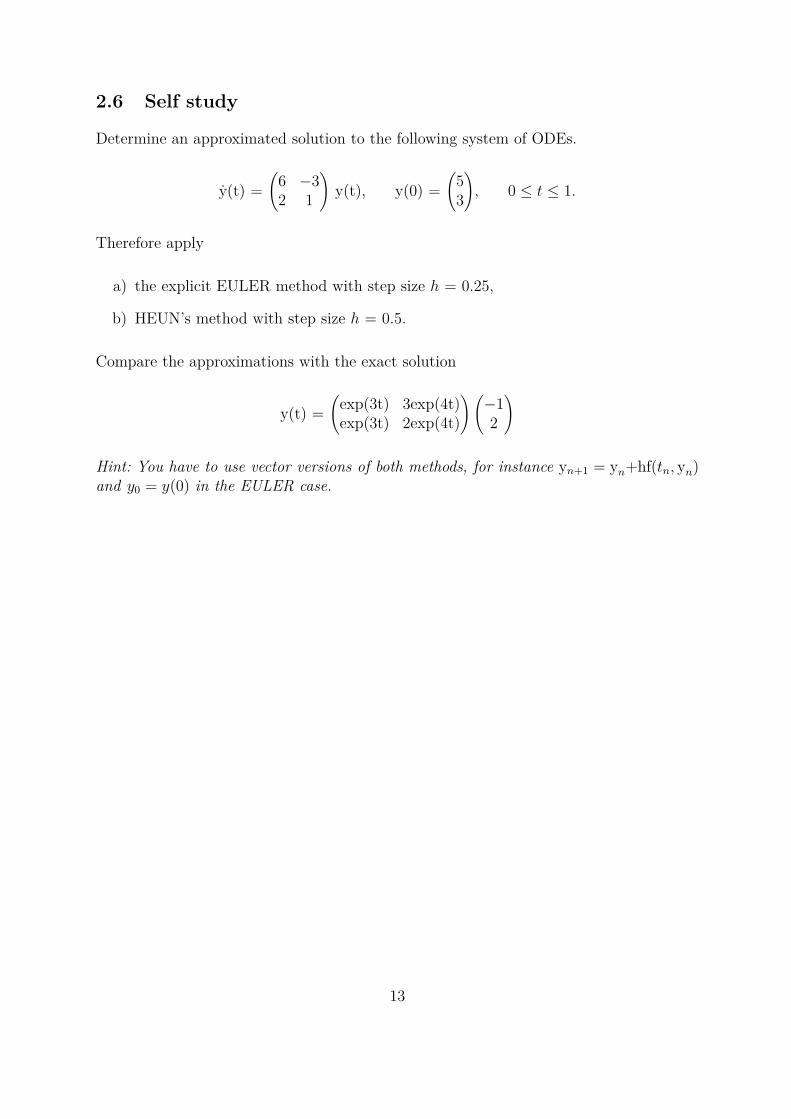
2.6 Self study

Determine an approximated solution to the following system of ODEs.

y(t) =(

6 −32 1

)y(t), y(0) =

(53

), 0 ≤ t ≤ 1.

Therefore apply

a) the explicit EULER method with step size h = 0.25,

b) HEUN’s method with step size h = 0.5.

Compare the approximations with the exact solution

y(t) =(

exp(3t) 3exp(4t)exp(3t) 2exp(4t)

)(−12

)

Hint: You have to use vector versions of both methods, for instance yn+1 = yn+hf(tn, yn)and y0 = y(0) in the EULER case.

13

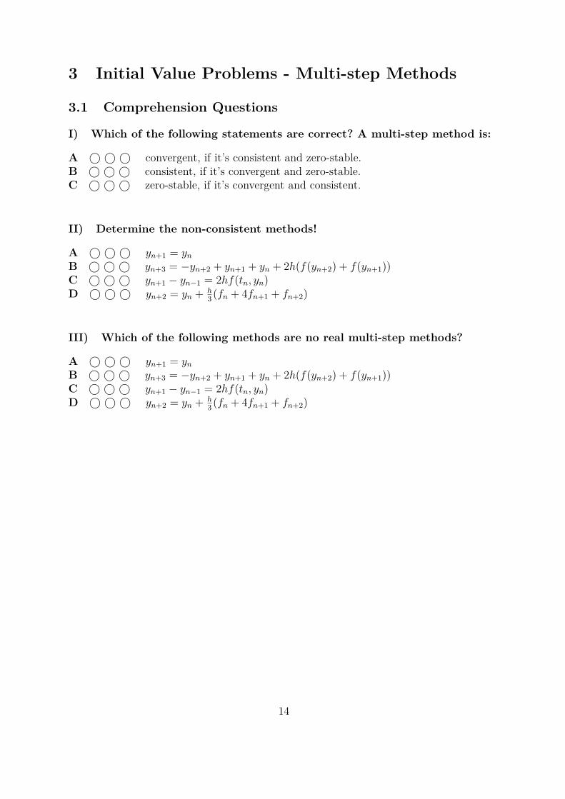
3 Initial Value Problems - Multi-step Methods

3.1 Comprehension Questions

I) Which of the following statements are correct? A multi-step method is:

A © © © convergent, if it’s consistent and zero-stable.B © © © consistent, if it’s convergent and zero-stable.C © © © zero-stable, if it’s convergent and consistent.

II) Determine the non-consistent methods!

A © © © yn+1 = ynB © © © yn+3 = −yn+2 + yn+1 + yn + 2h(f(yn+2) + f(yn+1))C © © © yn+1 − yn−1 = 2hf(tn, yn)D © © © yn+2 = yn + h

3 (fn + 4fn+1 + fn+2)

III) Which of the following methods are no real multi-step methods?

A © © © yn+1 = ynB © © © yn+3 = −yn+2 + yn+1 + yn + 2h(f(yn+2) + f(yn+1))C © © © yn+1 − yn−1 = 2hf(tn, yn)D © © © yn+2 = yn + h

3 (fn + 4fn+1 + fn+2)

14

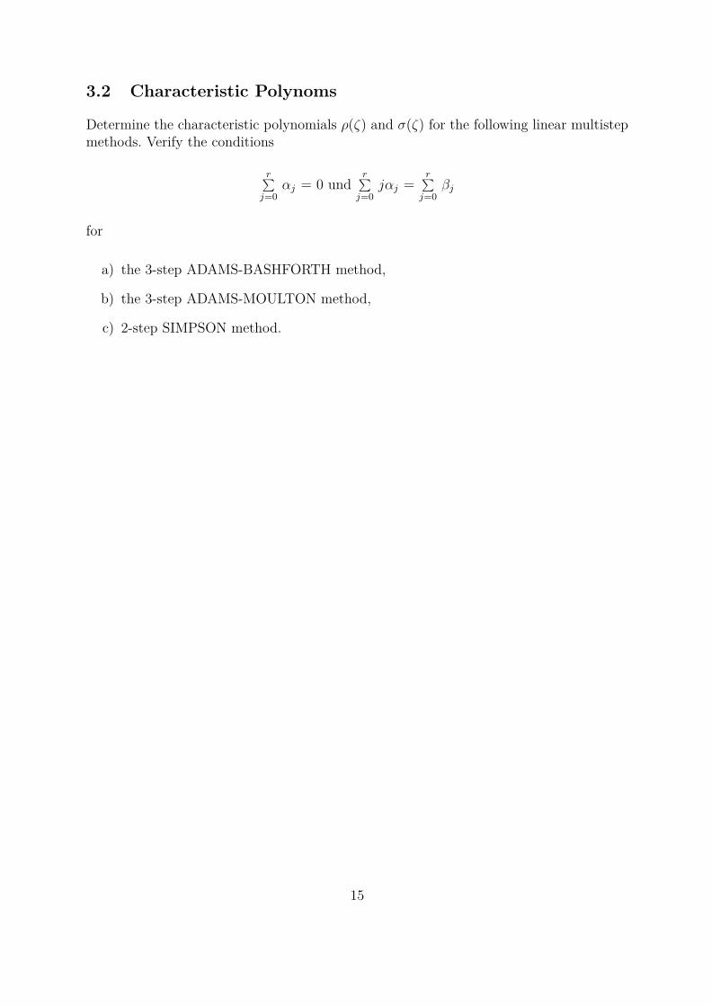
3.2 Characteristic Polynoms

Determine the characteristic polynomials ρ(ζ) and σ(ζ) for the following linear multistepmethods. Verify the conditions

r∑j=0

αj = 0 undr∑j=0

jαj =r∑j=0

βj

for

a) the 3-step ADAMS-BASHFORTH method,

b) the 3-step ADAMS-MOULTON method,

c) 2-step SIMPSON method.

15

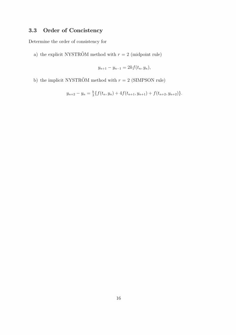
3.3 Order of Concistency

Determine the order of consistency for

a) the explicit NYSTROM method with r = 2 (midpoint rule)

yn+1 − yn−1 = 2hf(tn, yn),

b) the implicit NYSTROM method with r = 2 (SIMPSON rule)

yn+2 − yn = h3f(tn, yn) + 4f(tn+1, yn+1) + f(tn+2, yn+2).

16

3.4 Concistency, Zero-Stability & Convergence

Which of the following linear multistep methods are convergent? If a method is not con-vergent: is it consistent, not zero-stable, or both?

a) yn+2 = 12yn+1 + 1

2yn + 2hf(yn+1)

b) yn+1 = yn

c) yn+4 = yn + 43hf(yn+3) + f(yn+2) + f(yn+1)

d) yn+3 = −yn+2 + yn+1 + yn + 2hf(yn+2) + f(yn+1).

17

4 Initial Value Problems - MATLAB Training

Hint: This exercises should be done during the problem session in the PC-Lab MIB 2.10.Label the axes, titles and legend of the subplots comprehensibly.

4.1 Figures und Functions

Consider the initial value problem

y′(t) = t sin(2y), y(0) = π4 .

a) Approximate the exact solution

y(t) = arctan(et2)

on the time interval [0,3] with the modified EULER and HEUN‘s third-order methodusing self-defined functions. Draw figures of the exact and the numerical solutionsfor three different step sizes h<1.

b) Approximate the solutions with the explicit fourth-order ADAMS-BASHFORTHmethod. Take the first values of HEUN‘s method in a) as a startup and add thecurve into the 3 figures.

c) Draw a figure with logarithmic axes of the error maxi|yi − y(ti)| of the numericalsolutions for step sizes between 1 and 10−4.

18

4.2 Subplots and Function Handles

The ODEy′(t) = λ(y(t)− g(t)) + g′(t)

has the general solutiony(t) = Ceλt + g(t), C ∈ R

which, for Re λ < 0, consists on a decaying transient Ceλt and a steady state componentg(t). We consider the case g(t) = arctan t, λ = -10.

a) Draw a subplot of the general solution, i.e. plot the graph of y(t) for several choicesof C ∈ [-5,5].

b) Find the exact solution for the initial condition y(0) = 0.

c) Try to approximate the solution of this IVP with the explicit EULER method usingfunction handles. Plot the numerical solutions on the time interval [0,5] for h = 0.5,h = 0.25 and h = 0.1 in different subplots.

d) Repeat the experiment from (c) with the implicit EULER method using functionhandles and symbolic functions. Comment your observation.

19

5 Boundary Value Problems - Elliptic BVP

5.1 Comprehension Questions

I) Which of the following matrices describes the BVP -u′′(x) = 2,x ∈ Ω := (0,1), u(0) = 0, u′(1) = 0?

A © © ©(

2 −1−1 2

)(u1u2

)=(−2− 5

243−1− 40

243

)

B © © ©

2 −1 0−1 2 −11 −1 1

u1u2u3

=

−2− 5243

−1− 40243

13

C © © ©

2 −1 0−1 2 −10 −1 1

u1u2u3

=

−2− 5243

−1− 40243

23

II) Which of the following statements are wrong for the BVP -u′′(x) = 2,x ∈ Ω := (0,1), u(0) = 0, u′(1) = 0?

A © © © The BVP has two DIRICHLET boundary conditions!B © © © The BVP has a von NEUMANN boundary condition!C © © © The BVP is two-dimensional!D © © © The BVP is one-dimensional!

III) When discretizing a two-dimensional BVP the 5-point stencil is used.Which statement is NOT correct?

A © © © It’s also called 5-point discrete Laplacian!B © © © It can be derived from TAYLOR expansion forumula!C © © © It contains the 6 neighbors of each discretized point!D © © © This equation is not valid for boundary points!

20

5.2 DIRICHLET Boundaries

Consider the following elliptic boundary value problem of second order in the one dimen-sional space

-u′′(x) = -5x3 x ∈ Ω = (0,1)u(0) = -2;u(1) = -1

a) Check that u(x) = 14x

5 + 34x - 2 is the solution to the above boundary value problem.

b) Discretize the boundary value problem with central finite differences on a uniformgrid with mesh width ∆x = h = 1

3 .

Write down the associated linear system and determine a numerical approximationto the solution of the boundary value problem by solving this linear system.

c) Compare your numerical solution with the exact one.

21

5.3 Von NEUMANN Boundaries

Modify the boundary value problem from Exercise 5.2 to

-u′′(x) = -5x3 x ∈ Ω = (0,1)u(0) = -2;u′(1) = 2

a) Show, that u(x) = 14 x5 + 3

4 x - 2 is still a solution of this boundary value problem.

b) Discretize the boundary value problem with central finite differences on a uniformgrid with mesh width ∆x = h = 1

3 .

Write down the associated linear system and determine a numerical approximationto the solution of the boundary value problem by solving this linear system.

c) Compare your numerical solution with the exact one.

22

5.4 Universal Grid Size

Generate the matrices and right hand sides of Ax = b, when an arbitrary number of gridpoints is used. Try to simplify these matrices through (n+1) block structures?

23

5.5 DIRICHLET & von NEUMANN Boundaries

Consider the following second order elliptic boundary value problem in the one dimen-sional space

-u′′(x) = 2; x ∈ Ω := (0,1),u(0) = 0;u′(1) = 0;

a) Verify that the solution of the boundary value problem is given by u(x) = x(2− x).

b) Discretize the boundary value problem using central differences on a uniform gridwith mesh width ∆x = 1

3 . Write down the associated linear system and determine anumerical approximation to the solution of the boundary value problem by solvingthis linear system.

c) Compare your numerical solution with the exact one. What happens if the NEU-MANN boundary condition is replaced by u(1) = 0? Explain your observations.

24

5.6 Self Study

Determine the approximate stationary temperatur distribution in a thin quadratic metalplate with a side length of 0.5 m. Two adjacent are hold on a temperature of 0C. Onthe other boundaries are hold on a temperature of 0C to 100C.

(Hint: If x and y are the space coordinates, the problem can be describe by the stationaryheat equation ∆u(x,y) = 0 together with appropriate boundary value conditions. for thesolution of the linear system you should use software like MATLAB. for purposes ofcomparison notice, that the exact solution is given by u(x, y) = 400xy if the boundarieswith zero boundary condition are placed along the coordinate axes.)

25

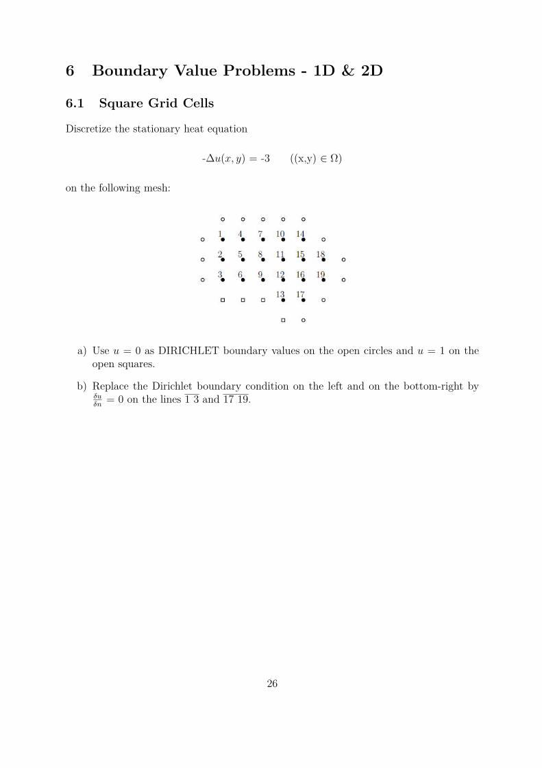
6 Boundary Value Problems - 1D & 2D

6.1 Square Grid Cells

Discretize the stationary heat equation

-∆u(x, y) = -3 ((x,y) ∈ Ω)

on the following mesh:

a) Use u = 0 as DIRICHLET boundary values on the open circles and u = 1 on theopen squares.

b) Replace the Dirichlet boundary condition on the left and on the bottom-right byδuδn

= 0 on the lines 1 3 and 17 19.

26

6.2 Rectangular Grid Cells

A rectangular silver plate of 6 cm x 5 cm is heated uniformly at each point with a constantenergy rate q = 6.2802 W/cm3. Assume that the temperature along the boundaries is holdat

u(x, 0) = x(6− x), u(x, 5) = 0 (0< x <6),u(0, y) = y(5− y), u(6, y) = 0 (0< y <5).

Then, the stationary temperature distribution can be described by the POISSON equation

∆u(x, y) = − qK

for (x, y) ∈ Ω := (0,6) × (0,5),

together with the above boundary conditions. The constant K = 4.3543 W/(cm· K) isthe thermal conductivity.

Approximate the temperature distribution by using the finite difference method with meshwidths ∆x = 0.4 and ∆y = 1

3 . Try also some other mesh widths.

27

6.3 Discretization in Space and Time

Consider the initial-boundary value problem

ut(x, y)− 12uxx(x, t) = 0 in Ω = (0,1) x (0,T),

u(x,=) = x(1− x) fur x ∈ (0,1),u(0, t) = u(1, t) = 0 fur t ∈ (0,T )

for an unknown function u = u(x;t).

a) Approximate u = u(x; t) at time t = 0.1 with an explicit difference scheme. Take astep size of ∆x = 0.25 in space and ∆t = 0.1 in time.

b) Approximate u = u(x, t) at time t = 0.1 with a purley implicit difference scheme.Take the same step size as in a).

c) For which step sizes ∆t in time is the explicit and the purely implicit differencescheme numerically stable, if a step size ∆x = 0.25 in space is provided?

28

7 Assignment - Restricted 3-Body Problem

We consider a satellite in the gravity field of earth and moon. We assume that the move-ment of the three bodies takes place within a fixed plane, and that the two heavy bodiesare rotating around their barycenter with constant distance and with constant angularvelocity. This means, the influence of the satellite on the orbits of earth and moon can beomitted - that’s why this is called a restricted 3-body problem.With respect to a coordinate system which is coupled to this rotation (i.e. earth andmoon have fixed positions in this system), the satellite’s orbit (x, y) = (x(t), y(t)) can bedescribed by a system of second order differential equations:

x′′ = x+ 2y′ − µ x+µ[(x+y)2+y2]3/2 − µ x−µ

[(x−µ)2+y2]3/2

y′′ = y − 2x′ − µ y[(x+µ)2+y2]3/2 − µ y

[(x−µ)2+y2]3/2

Here µ = 1/82.45 is the ration between the mass of the moon and the cumulative mass ofearth and moon, and µ = 1 - µ. The length unit is the distance between earth and moon.The earth is placed in the origin and the moon on the positive real axis. The time unit ischosen in a way, that the angular velocity of the rotation is one, i.e. the moon needs 2πtime units for one orbit.

a) Rewrite the second order differential equation system as a first order system. Applythe substitutions y1(t) = x(t), y2(t) = y(t) and y3(t) = x′(t), y4(t) = y′(t).

b) Solve the first order ODE system using the MATLAB routine

[t,y] = ode45(@f,y0,[0 tend],options)

with the following initial values y0 in t = 0:

y1(0) = 1.2, y2(0) = 0, y3(0) = 0, y4(0) = -1.04935750983031990726

Therefore chosen and appropriate end tend for the integration interval.

29

c) Specify or control via the fourth input parameter options:

- the tolerances RelTol and AbsTol for the stepsize control of ode45,- the plot function for the phase plot (y1, y2) (corresponds to (x(t), y(t))),- the detection of local minima and maxima of the orbit/trajectory (points with

horizontal or vertical tangent) by use of an event function.Hint: Analyze the additional output parameters in the statement[t,y,te,ye,ie] = ode45(@f,y0,[0 tend],options).

d) Observe what happens if

- tend will be enlarged or reduced,- the fourth component in the initial condition y4(0) is rounded (for instance)

to -1.05

e) Modify the event function so that ode45 terminates after the calculation of a closedtrajectory.

f) Solve the 3-body problem with a classical RUNGE-KUTTA method of fourth orderan constant stepsize h = (tend− t0)/n. How many integration steps n are needed toget a similar trajectory as with ode45?

Use the plot statement to generate a picture of the orbital trajectory.

g) Solve the 3-body problem a second time with ode45 using the following data

µ = 0.012277471,y1(0) = 0.994, y2(0) = 0, y3(0) = 0, y4(0) = -2.00158510637908252240537862224.

Determine a value for tend resulting in a closed trajectory. How many integrationsteps are needed for the associated integration interval?Hint: The number of integration steps in ode45 depends on the chosen tolerancesRelTol and AbsTol.

h) Try to reproduce the second orbit with the classical RUNGE-KUTTA method withfixed stepsize.

30