Exercise 6 - WinHSPF Hydrology Calibration · BASINS/HSPF Training Exercises 6-1 Exercise 6 - WinHSPF Hydrology Calibration Water Quality Calibration/ Validation Parameter Development/Model

BASINS/HSPF Training Exercises

6-1

Exercise 6 - WinHSPF Hydrology Calibration

Water Quality Calibration/ V alidation

Parameter Development/Model

Setup

H yd r ologic Ca lib r a t ion /

Va lida t ion

T imeseries Data M anagement

Study Definition/Modeling

StrategyScenario A nalysis

BASINS/HSPF Application Steps

Water Quality Calibration/ V alidation

Parameter Development/Model

Setup

H yd r ologic Ca lib r a t ion /

Va lida t ion

T imeseries Data M anagement

Study Definition/Modeling

StrategyScenario A nalysis

BASINS/HSPF Application Steps

The goal of calibration is to “tune” the model so that the simulated flow resembles the observed flow data as closely as possible. This is accomplished by adjusting various input parameters within WinHSPF. In this computer discussion, we will discuss many of the key calibration parameters. The most important thing to remember is that the estimated values of each parameter should be realistic and make physical sense. Appendix B explains some of the important site-specific parameters that need to be entered into WinHSPF before calibrating the hydrology. This information includes F-tables, local weather data, and topography information. In order to save time, we have entered these inputs for the West Branch Patuxent model. We will open and use an updated project for this exercise. Before we begin calibrating, we will run the input file (*.uci) that contains the updated site-specific information. After we have looked at the simulated flow output, we will adjust the values of some important calibration parameters and look at how those changes affect the simulated flow. A. Before Calibration 1. If WinHSPF isn’t open, from the Start menu under Programs, select BASINS and

then WinHSPF.

2. Click (Open File). 3. Navigate to c:\basins\modelout\Man_Cal and select “hyd_man.” Click OPEN. The best way to begin the calibration process is to look at the annual total runoff volume error. In this section, we will compare the total annual simulated flow volumes to the total annual observed flow volumes. In the following steps, we will specify that we want the total annual simulated flow to be printed to the output file. We will compare these volumes to the observed flow volumes.

4. Click (Input Data Editor).

5. Double click RCHRES GENERAL PRINT-INFO.


6-2

Note: In the “PRINT-INFO” screen, you can specify which output will be printed to the output file (man_cal.out). You can also specify the print frequency for each reach and constituent. We want to look at the annual total simulated volumes for Reach 5. Since we are modeling only hydrology in this exercise, we need to specify the print frequency for only the column “HYDRPR.”

6. In the cell that corresponds to the column “HYDRPR” and Reach 5 (Western Branch Patuxent), change the value to “5.” Change the rest of the values in the “HYDRPR” column to “6.”

Note: A value of 5 means that the total flow volumes for Reach 5 will be printed for

each year. The total volumes for the other reaches will not be printed to the output file. Your screen should look like the following:

7. Scroll to the right until you see the “PYREND” column. Click in the first cell in this


6-3

column. Change the value to “12” and double click the column heading to copy the values to the rest of the column.

Note: By assigning “PYREND” a value of “12,” we are specifying that the year will

end in December. In other words, the total flow will be printed each year for January 1 to December 31. If you specified “10” as the value for “PYREND,” the total flow for November 1 to October 31 of the next year would be printed in the output file.

8. Click APPLY.

9. Click OK.

10. Click CLOSE.

11. Click (Run HSPF).

12. Click SAVE/RUN. The following window will appear, indicating that HSPF is

executing.

13. Click (View Output through GENSCN). 14. Click the “HSPF Output” tab.


6-4

15. Check the box beside “c:\BASINS\modelout\hyd_out.WDM” and click OK. The

GenScn window will open. 16. In the “Scenarios” frame, select “HYD_MAN” and “OBSERVED.” 17. In the “Constituents” frame, select “FLOW.”

18. Click (Add to Time-Series List). 19. In the “Time Series” frame, select the “hyd_man” and “observed” time series by

holding the shift key while selecting them. Your screen should look like this:

20. Click (Generate Graphs).

21. Check the boxes beside “Standard,” “Flow/Duration,” “Scatter (TS2 vs. TS1)” and “45 deg/regress lines.”


6-5

22. Click GENERATE.

Note: When you click GENERATE, three plots will appear. The “Scatter” plot will be in front and the “Standard” (flow) plot will be in back.

23. Click on the “Genscn Standard Plot” window.

Notice the difference between the observed (OBSERVED UPMARLBR) and simulated (HYD_MAN RCH5) flow data. To look more closely at the difference, we will look at a smaller range of flow values.

24. Move your cursor over the “FLOW” axis and double click. The following window will appear:


6-6

25. Make sure the “Axes” tab is selected. In the “Left Y-axis” frame under the “Axis Scale Range,” change the “Max” to “400.”

26. Click APPLY.

27. Click OK. Your plot should look like the following:

28. Close the “Genscn Standard Plot” window. 29. Click on the “Genscn FLOW/Duration Plot” window.


6-7

Note: This plot is a cumulative frequency plot. It shows how well the two series correlate in frequency. For each frequency in the range from 0 to 100 percent (X-axis), the flow that will be exceeded that percent of the time is plotted on the Y-axis. Ideally, the two curves should be very similar. Notice that the curves don’t match well at the tails - high flow points (over 100 cfs) and low flow points (below10 cfs).

30. Close the “Genscn FLOW/Duration Plot” window.

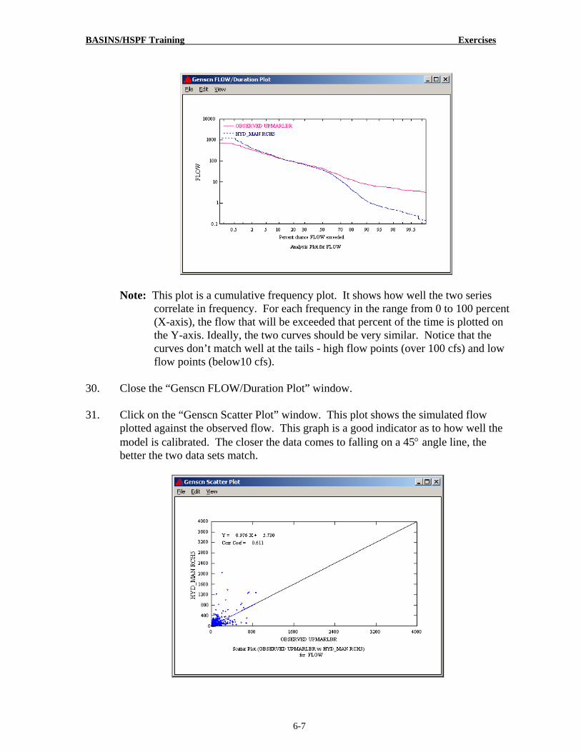
31. Click on the “Genscn Scatter Plot” window. This plot shows the simulated flow plotted against the observed flow. This graph is a good indicator as to how well the model is calibrated. The closer the data comes to falling on a 45° angle line, the better the two data sets match.


6-8

32. Close the “Genscn Scatter Plot” window.

33. Close GenScn. Do not save changes.

In the next section, we will begin the calibration process. We will adjust the values of some parameters and ascertain the effects by re-running the model and viewing the results. B. Total Runoff Volume Error – LZSN and UZSN The best way to begin the hydrology calibration process is to examine the total runoff volume error. This type of analysis should be performed for the following time periods:

• Annual • Seasonal • Monthly • Storm periods

You can compute the total runoff volume error for a specific time period by estimating the total volume of water passing through a reach according to the gage data (observed flow) and comparing it to the output volume simulated by the WinHSPF model (simulated flow). Volume = Σ Q*∆t Once the simulated and observed volumes have been calculated and compared, you can adjust the values of calibration parameters until the total annual simulated volumes are very close to the total annual observed volumes. Losses in the watershed can be accounted for by quantifying flow diversions, evapotranspiration losses, and losses due to deep percolation. For this model, we will assume that we have accounted for all flow diversions and that losses due to deep percolation are negligible. We will therefore assume that all losses are due to evapotranspiration and adjust parameters that are associated with evapotranspiration. LZSN (lower zone storage nominal) is related to precipitation and soil characteristics in the watershed. Increasing the value of LZSN increases the amount of water stored in the lower zone and therefore, increases the opportunity for evapotranspiration. This decreases flow rates by providing greater opportunity for evapotranspiration. Decreasing the value of LZSN increases flow rates in the reach. UZSN (upper zone storage nominal) is related to land surface characteristics, topography, and LZSN. This parameter can change over the course of a growing season. Increasing UZSN increases the amount of water retained in the upper zone and available for evapotranspiration, allowing less overland flow. Some suggestions for UZSN are (BASINS Technical Note 6):


6-9

• 0.06*LZSN – steep slopes and limited vegetation • 0.08*LZSN – moderate slopes and vegetation • 0.14*LZSN – mild slopes and heavy forest cover

Other parameters that may impact the error in total runoff are FOREST, PETMAX, PETMIN, and DEEPFR. The following section is designed to illustrate how changes in LZSN and UZSN affect the simulated stream flow hydrograph in WinHSPF. Before we begin calibration, we will look at the output file, compare the total annual simulated flow volumes to the total annual observed flow volumes, and determine whether our calibration efforts should focus on increasing or decreasing the total annual simulated flow volume. Annual Total Runoff Volume Error 1. Open Windows Explorer or My Computer (do not close WinHSPF).

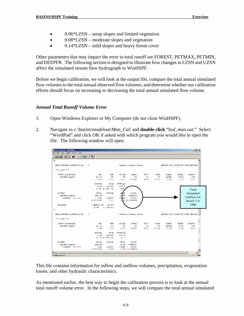
2. Navigate to c:\basins\modelout\Man_Cal\ and double click “hyd_man.out.” Select

“WordPad” and click OK if asked with which program you would like to open the file. The following window will open:

This file contains information for inflow and outflow volumes, precipitation, evaporation losses, and other hydraulic characteristics. As mentioned earlier, the best way to begin the calibration process is to look at the annual total runoff volume error. In the following steps, we will compare the total annual simulated

Total Simulated

Outflow for Reach 5 in

1986


6-10

flow volumes to the total annual observed flow volumes. The total annual simulated flow volumes (acre-ft) can be found in the output file hyd_man.out (shown above). They are listed under the heading “TOTAL OUTFLOW ROVOL.” The project *.wdm file (hyd_out.wdm) contains the daily observed flow data (cfs) for Reach 5. These data must be converted to total annual flow volumes. In order to save time, this has already been done. For conversion details, see Appendix C.

The following table shows the comparison of observed and simulated annual flow volumes (acre-ft):

Date Simulated Outflow

Observed Outflow

Percent Difference

1986 49,740 40,632 22.42 1987 55,120 53,264 3.48 1988 47,420 49,400 -4.01 Total 152,280 143,296 6.27

The error in total volume for the three-year time period is relatively good (within 10%). We will adjust some parameters in order to bring the two values even closer. Since we are over predicting flow volumes, we want to increase losses in the watershed. We will do this by increasing the evapotranspiration loss. Close WordPad when you are done.

3. Click (Data Editor).

4. Double click “PERLND,” then “PWATER,” and then “PWAT-PARM2.”

5. Click in the first cell in the column “LZSN” and enter “14.” Double click the column heading to fill in the values for the rest of the column. Note: According to BASINS Technical Note 6, the value of possible ranges for LZSN

is 2 to 15 inches. We are entering “14,” a number that is unrealistic for the West Patuxent watershed, to illustrate how changing the value of LZSN will affect the total runoff volumes.

Note: In normal modeling situations, you should vary the parameter as appropriate

by land use. For simplification purposes, we are using the same LZSN value for all land uses, but this is not appropriate practice in actual model application.


6-11

6. Click APPLY.

7. Click OK. 8. Click CLOSE.

9. Click (Run). 10. Click SAVE/RUN.

11. Click (View Output through GENSCN). 12. Follow steps 16-33 in Section A to look at the output. Your plots should look like

the following:


6-12

13. Close all of the plot windows. 14. Close the “Generate Plots” window. 15. Close GenScn. Do not save changes. 16. Open “Windows Explorer” or “My Computer.” 17. Navigate to c:\basins\modelout\Man_Cal\ and double click “hyd_man.out.” Look at

the modified annual flows. The updated comparison of annual flow volumes (acre-ft) is as follows:


Observed Outflow

Percent Difference

1986 29,920 40,632 -26.36 1987 40,050 53,264 -24.81 1988 35,680 49,400 -27.77 Total 105,650 143,296 -26.27

Overall, there is a 26.27% difference between annual simulated and observed flow volumes. Before we adjusted the value of LZSN, the simulated flow was too high; now it is too low. This means we increased the value of LZSN too much. We will decrease the value.

18. Click (Data Editor). 19. Double click PERLND, PWATER, and then PWAT – PARM 2 (PERLND

PWATER PWAT-PARM 2). 20. Change each value in the “LZSN” column to “5.” 21. Click APPLY. 22. Click OK. 23. Click CLOSE.

24. Click (Run). 25. Click SAVE/RUN.

26. Click (View Output through GENSCN). 27. Follow steps 16-33 in Section A to view the output in GenScn. The GenScn plots


6-13

should look like the following:

If you wish, you can open and view the output file (hyd_man.out). The updated comparison of annual flow volumes(acre-ft) is as follows:


Observed Outflow

Percent Difference

1986 46,720 40,632 14.98 1987 51,760 53,264 -2.82 1988 44,640 49,400 -9.64 Total 143,120 143,296 -0.12

The overall total runoff volume error is 0.12%. This is very good, so we will move on to the seasonal volume error. We will look at the winter (December – February) water volumes and summer (June – August) water volumes. Seasonal Statistics Before we adjust any parameter values, we will look at the current seasonal statistics. In order to look at the statistics for the summer months and winter months, we need to change the output print frequency to “months.” 28. In the WinHSPF Data Editor window, double click RCHRES GENERAL

PRINT-INFO.


6-14

29. In the “HYDRPR” column, change the value that corresponds to Reach 5 to “4.”

This specifies that we would like to see the monthly results for Reach 5 in the output file (see parameter definition near the bottom of the Data Editor window). Leave all other values at 6.

30. Click APPLY.

31. Click OK.

32. Click CLOSE.

33. Click (Run).

34. Using My Computer or Windows Explorer, open “hyd_man.out.” Scroll through the file. Notice that the file includes both total monthly volumes and total annual volumes.

In previous steps, we looked at the annual volume error and adjusted the value of LZSN so that the simulated flow volumes would more closely resemble the observed flow volumes. We will now look at the winter and summer flow volumes (acre-ft). The following table shows the seasonal statistics:


6-15

Year Month Sim. Flow Obs. Flow % Diff. Month Sim. Flow Obs. Flow % Diff. 1986 January 4,855 June 607

February 8,719 July 1,959

August 2,785

Winter: 13,574 10,181 33.33 Summer: 5,351 5,188 3.14

December 14,210 June 3,114

1987 January 10,990 July 1,197

February 4,802 August 921

Winter: 30,002 25,517 17.58 Summer: 5,232 4,273 22.44


1988 January 7,838 July 1,791

February 8,914 August 1,603

Winter: 22,921 22,076 3.83 Summer: 4,909 5,428 -9.56

Total Winter: 66,497 57,775 15.10 Total Summer: 15,492 14,889 4.05

Notice that there is a 4.05% difference between the total observed and total simulated flow volumes for summer, but there is a 15.10% difference for winter flows. In general, the upper zone storage is near capacity in the winter and there is little evapotranspiration occurring so the value of the nominal storage (UZSN) has a minimal effect in winter, but a much larger effect during summer when losses from the upper zone storage are at or near the potential due to high evapotranspiration rates. In the case of this exercise, the summer flows are almost entirely dominated by base flow, so the upper zone storage (which is controlled by UZSN) is empty the majority of the time, even during summer storm events. To move forward with this exercise, we will raise UZSN for the non-agricultural land uses. Note that because VUZFG is 1 for PERLND 103 (agricultural land), the values of UZSN actually being used for agricultural land are in the table MON-UZSN. Thus changing the values of UZSN in the table PWAT-PARM4 affects only the non-agricultural land uses.

35. Click the “Data Input Manager” button, .

36. Double click PERLND PWATER PWAT-PARM4.

37. Change all the values in the “UZSN” column to “1.8.”

38. Click APPLY.

39. Click OK. 40. Click CLOSE.


6-16

41. Click (Run). The winter and summer statistics is as follows:

Year Month Sim. Flow Obs. Flow % Diff. Month Sim. Flow Obs. Flow % Diff. 1986 January 4,633 June 608

February 7,322 July 1,960

August 2,782

Winter: 11,955 10,181 17.42 Summer: 5,350 5,188 3.12


1987 January 10,370 July 1,195

February 4,851 August 928

Winter: 27,681 25,517 8.48 Summer: 5,167 4,273 20.92


1988 January 7,253 July 1,787

February 8,449 August 1,605

Winter: 21,342 22,076 -3.32 Summer: 4,866 5,428 -10.35

Total Winter: 60,978 57,775 5.54 Total Summer: 15,383 14,889 3.32

The total summer difference has only changed slightly (from 4.05% to 3.32%), but the total winter difference is down to 5.54 %. This percent difference is good enough for our purposes. In our simulation, we increased evapotranspiration significantly for the winter months. Since this will surely have an effect on the annual statistics, we will look at the total annual flow volumes (acre-ft) for this simulation. They are as follows:


Observed Outflow

Percent Difference

1986 42,620 40,632 4.89 1987 49,790 53,264 -6.52 1988 42,990 49,400 -12.98 Total 135,400 143,296 -5.51

This is acceptable, since the total percent difference is still lower than 10%. The next step is to complete statistics for each month and adjust parameters as needed. It is possible to have monthly values for many of the parameters. After the monthly statistics, it is best to look at the storm statistics. You can complete the monthly comparison and the storm comparison by using the method outlined above. In order to save time, we will move on to high and low flows.


6-17

C. Soil Moisture Storage and Actual Evapotranspiration (High and Low Flows) – INFILT and LZETP

Soil moisture storage is important because it controls the division between surface and subsurface flow (Hydrologic Journal) and affects the timing of the runoff and statistics. INFILT is an index to mean soil infiltration rate. It is a function of soil characteristics and controls how much of the water from precipitation will become surface flow, subsurface flow, and a portion of the storage components. Increasing the value of INFILT produces more water in the lower zone and therefore, generally results in higher base flow in the streams. Low values of INFILT will produce more upper zone and interflow storage water, resulting in greater direct overland flow (if the upper zone is saturated) and interflow (BASINS Technical Note 6). INFILT is closely related to LZSN, UZSN, AGWRC, IRC, and KVARY, since the value of INFILT will determine the allocation of water in the soil profile. LZETP (index to lower zone evapotranspiration) is a coefficient (unitless) used to define the opportunity for evapotranspiration. It affects the amount of evapotranspiration from the lower zone, which represents the primary soil moisture storage and root zone of the soil profile. This parameter behaves like a crop coefficient (BASINS Technical Note 6). We are going to view the output from the last run in GenScn. Look at the peak flows and base flows and try to determine whether there are any patterns.

1. Make sure “hyd_man.uci” is active in WinHSPF

2. Click the “View Output Through GenScn” button, .

3. In the “Scenarios” frame, select “HYD_MAN” and “OBSERVED.”

4. In the “Constituents” frame, select “FLOW.”

5. Click (Add to Time-Series List).

6. In the “Time Series” frame, select the “hyd_man” and “observed” time series by holding the shift key while selecting them.

7. In order to see patterns more clearly, we will look at the flow plot for only one year. In the “Dates” frame, change the “Start” date to “01-01-1988.”


6-18


9. Make sure the box beside “Standard” is checked and click GENERATE. Double click somewhere on the “FLOW” axis.

10. In the “Left Y-axis” frame, change the “Max:” value to “500.” Click APPLY and then OK.

The plot should look similar to the following:

The following table shows the simulated high and low flow volumes compared to the observed high and low flow volumes:


6-19

Simulated Observed % Diff. ∑ High Flows: (upper 10%) 22566 29448 -23.37 ∑ Low Flows: (lower 50%) 3229 10059 -67.90

Notice that the simulated base flow is consistently lower than the observed base flow. In order to help increase the base flow in our model, we need to allocate more interflow and groundwater and less surface runoff to stream flow. We will do this by increasing the value of “INFILT.” 11. Close the plot windows and exit GenScn. Do not save changes.

12. In WinHSPF, click (Data Editor).

13. Double click PERLND PWATER PWAT-PARM2. Change the values in the “INFILT” column to “0.5.”

14. Click APPLY.

15. Click OK.

16. Click CLOSE to exit the “Input Data Editor.”

17. Click (Run). 18. After the model has finished executing, follow steps 2-11 (in this section) to view the

output graphically. The flow plot should look like the following:

The following table shows the adjusted high and low flow volume comparison:

Observed Simulated % Diff. ∑ High Flows: (upper 10%) 29448 32966 11.95 ∑ Low Flows: (lower 50%) 10059 6353 -36.84


6-20

The “low flow” comparison improved (from –67.9% to –36.84%). We still need to improve our low flow numbers, but we have already increased the value of INFILT to the maximum value recommended in BASINS Technical Note 6. In the next section, we will adjust other parameters in order to improve our high and low flow volume errors. D. Seasonal and Low Flows – KVARY and AGWRC Seasonal and low flows are simulated by changing the volume of water flowing through the groundwater path and interflow paths in your model. Recall that adjusting INFILT value(s) will change the distribution of water that will flow through the upper zone and that this parameter value works with others (LZSN, UZSN, AGWRC, KVARY, IRC) to determine the allocation and timing of surface runoff, interflow, and groundwater contributing to stream flow. Seasonal flows can also be adjusted by changing the recession rate for flows entering the reach via groundwater paths. AGWRC is the groundwater recession rate. It is the ratio of current groundwater discharge to that from 24 hours earlier when KVARY is zero. KVARY is the groundwater recession flow parameter that describes non-linear groundwater recession rates. It is usually one of the last parameters adjusted and is used when the observed groundwater recession demonstrates a seasonal variability with a faster recession during wet periods and the opposite during dry periods. Users should begin with a KVARY value of 0.0 and then increase if there are seasonal variations. Since our simulated base flow is still too low, we will increase the value of AGWRC.

1. Click (Data Editor). 2. Double click PERLND PWATER PWAT-PARM2.

3. Change each value in the “AGWRC” column to “0.99.” 4. Click OK. 5. Click APPLY. 6. Click CLOSE.

7. Click (Run). The adjusted high/low flow volumes are as follows:


6-21

Observed Simulated % Dif. ∑ High Flows: (upper 10%) 29448 31854 8.17 ∑ Low Flows: (lower 50%) 10059 9893 -1.65

Since both the high and low flow percent differences are considerably better than before, and sufficient for our purposes, we will not adjust the value of KVARY. We will now look at the shape of our storm peak flows. E. Hydrograph Shape and Peak Flows – INTFW and IRC Hydrograph shape is affected by the relative magnitudes of surface runoff and interflow among and within watersheds. The coefficients INTFW and IRC control the amount and timing of water that will enter the reach as interflow. Channel cross-sections and the slope and distance of the overland flow plain are also important in hydrograph shape and peak flows in some watersheds. For watersheds in which the channel flow-thru time is 10 minutes or less, the overland flow parameters (LSUR, SLSUR, and NSUR) are important for hydrograph shape and peak flows. (Hydrologic Journal). INTFW is the coefficient that determines how much water will enter the ground from detention storage and become interflow (instead of direct overland flow and upper zone storage). INTFW has an effect on the timing of runoff by controlling the division of water between interflow and surface processes. Increasing the value of INTFW increases the amount of interflow, decreases direct overland flow and thereby reduces the peak flows while maintaining the same volume. It alters the shape of the hydrograph by shifting and delaying the flow to later in time. Decreasing INTFW has the opposite affect (raises the peaks). Base flow is not affected by INTFW. Once storm volumes have been calibrated, INTFW can be used to raise or lower peaks to match the observed hydrograph (BASINS Technical Note 6). IRC is the interflow recession coefficient. It is analogous to the groundwater recession parameter (AGWRC) and is the ratio of current daily interflow to the interflow discharge on the previous day (24 hours earlier). IRC affects the rate at which interflow is discharged from storage, so it affects the shape of the hydrograph by altering the “falling” phase (recession region) of the curve between the peak storm flow and baseflow. IRC can be adjusted based on whether simulated storm peaks recede faster / slower than observed after AGWRC has been calibrated (BASINS Technical Note 6). We are going to plot the results of the last simulation we ran. As you look at the plot, notice the shape of the peak flows. 1. Follow steps 2-11 in Section C to view the plot. Your flow graph should look similar

to the following:


6-22

Note: Notice that the peak recession is occurring too quickly. We will increase the value of “INTFW” in order to slow down the recession rate and flatten the peaks a little.

2. Click (Data Editor).

3. Double click PERLND PWATER PWAT-PARM4.

4. Click in the first cell of the column “INTFW.” Change the value to “3” and then double click the column heading to copy the values for the rest of the column.

5. Click APPLY.

6. Click OK.

7. Click CLOSE.

8. Click (Run).

9. Follow steps 2-11 in Section C to view the results in GenScn. Your flow plot should look similar to the following:


6-23

Note: Notice that the peak recessions are occurring more gradually. You can continue to change the values of various parameters to more finely calibrate the model. Keep in mind that this is a fairly rough calibration that was designed to illustrate the principles of calibration. In your own calibration efforts, it is important to perform statistics on the monthly and storm flow volumes (in addition to the annual and seasonal statistics), adjust parameter values in small increments, and take the time to make sure the parameter values truly represent your watershed. We will look at the plots for the entire time period to see how our model has changed. 10. Close the plot window and return to the main window of GenScn. In the “Dates”

frame, change the “Start” date to “01-01-1986.”


12. Check the boxes beside “Standard,” “Flow/Duration,” “Scatter (TS2 vs. TS1)” and “45 deg/regress lines.” Click GENERATE.


6-24

The plots should look like the following:

Notice that the two lines (simulated and observed) now line up very well.


6-25

The variability shown on this graph is due mostly to extreme points in our hydrograph. The model takes into account all points when producing the linear regression equation. 13. Exit GenScn. F. Additional Calibration Requirements When calibrating hydrology, it is important to examine the overall water balance within each land segment. This effort involves displaying and analyzing model results for individual land uses for the following water balance components: rainfall, runoff (including surface runoff, interflow, and baseflow), evaporation losses (including potential, interception, upper zone, lower zone, baseflow, and active groundwater), and deep groundwater recharge/losses. Although observed values are not available for each of the water balance components listed above, the average annual values must be consistent with expected values for the region, as impacted by the individual land use categories. This is a separate consistency, or reality, check with data independent of the modeling (except for precipitation) to insure that land use categories and overall water balance reflect local conditions. It is recommended that you create a table similar to the following for each land use when calibrating flow for your watershed. This table will help you compare the runoff and evaporation components among land uses and make sure that they are logical and consistent. This table is presented only as an example. Water Balance Components for Agriculture, PERLND 101, in inches:

Date 1990 1991 1992 1993 1994 1995 AverageRainfall 41.87 35.52 35.28 49.27 37.24 44.17 40.56

Runoff Surface 0.10 0.12 0.16 0.80 0.15 0.81 0.35

Interflow 1.94 1.71 1.89 6.88 2.25 3.98 3.11

Baseflow 9.70 8.33 8.92 14.92 8.65 10.82 10.22

Total 11.73 10.16 10.96 22.59 11.05 15.61 13.68

Deep Groundwater 0.00 0.00 0.00 0.00 0.00 0.00 0.00

Evaporation Potential 31.69 35.44 29.38 30.44 33.19 34.09 32.37

Intercep St 9.34 8.37 8.30 10.05 8.53 9.28 8.98

Upper Zone 7.59 5.94 4.29 9.34 6.32 8.17 6.94

Lower Zone 9.70 11.17 10.65 8.10 11.11 10.74 10.24

Ground Water 0.00 0.00 0.00 0.00 0.00 0.00 0.00

Baseflow 0.32 0.32 0.28 0.30 0.32 0.34 0.31

Total 26.94 25.80 23.52 27.78 26.27 28.53 26.47


6-26

GenScn has a built-in scripting capability to produce summary tables from HSPF output. In this portion of the exercise we will use the scripting capability to build a water balance component summary like the one above.

1. Make sure “hyd_man.uci” is open in WinHSPF and click the “View Output Through GenScn” button.

2. From the Analysis menu, choose the option Run Script.

3. From the script selection window, go to c:\BASINS\models\HSPF\bin and select the script “GenScnWaterBalance.spt.” Click OPEN.

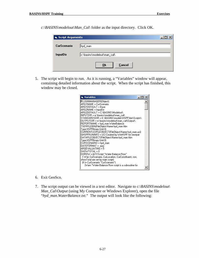
4. Type “hyd_man” in the “CurScenario” (or current scenario) box, and specify the


6-27

c:\BASINS\modelout\Man_Cal\ folder as the input directory. Click OK.

5. The script will begin to run. As it is running, a “Variables” window will appear, containing detailed information about the script. When the script has finished, this window may be closed.

6. Exit GenScn. 7. The script output can be viewed in a text editor. Navigate to c:\BASINS\modelout\

Man_Cal\Output (using My Computer or Windows Explorer), open the file “hyd_man.WaterBalance.txt.” The output will look like the following:


6-28

References: BASINS Technical Note 6, Estimating Hydrology Parameters for NPSM/HSPF – DRAFT.

September 15, 1999. Hydrologic Journal, http://www.hydrocomp.com/journal4.htm. Hydrocomp, Inc.

Documents

Exercise 6 - WinHSPF Hydrology Calibration · BASINS/HSPF Training Exercises 6-1 Exercise 6 - WinHSPF Hydrology Calibration Water Quality Calibration/ Validation Parameter Development/Model