1

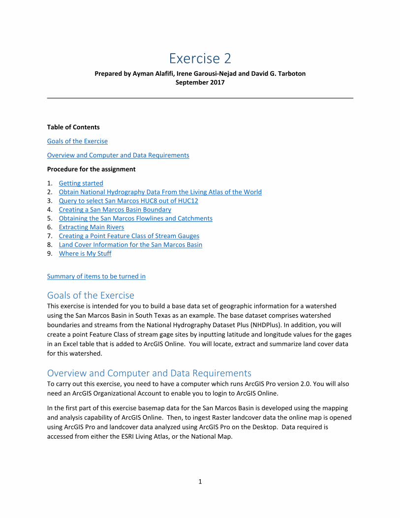
Exercise 2 Prepared by Ayman Alafifi, Irene Garousi-Nejad and David G. Tarboton

September 2017

Table of Contents

Goals of the Exercise

Overview and Computer and Data Requirements

Procedure for the assignment

1. Getting started 2. Obtain National Hydrography Data From the Living Atlas of the World 3. Query to select San Marcos HUC8 out of HUC12 4. Creating a San Marcos Basin Boundary 5. Obtaining the San Marcos Flowlines and Catchments 6. Extracting Main Rivers 7. Creating a Point Feature Class of Stream Gauges 8. Land Cover Information for the San Marcos Basin 9. Where is My Stuff

Summary of items to be turned in

Goals of the Exercise This exercise is intended for you to build a base data set of geographic information for a watershed using the San Marcos Basin in South Texas as an example. The base dataset comprises watershed boundaries and streams from the National Hydrography Dataset Plus (NHDPlus). In addition, you will create a point Feature Class of stream gage sites by inputting latitude and longitude values for the gages in an Excel table that is added to ArcGIS Online. You will locate, extract and summarize land cover data for this watershed.

Overview and Computer and Data Requirements To carry out this exercise, you need to have a computer which runs ArcGIS Pro version 2.0. You will also need an ArcGIS Organizational Account to enable you to login to ArcGIS Online.

In the first part of this exercise basemap data for the San Marcos Basin is developed using the mapping and analysis capability of ArcGIS Online. Then, to ingest Raster landcover data the online map is opened using ArcGIS Pro and landcover data analyzed using ArcGIS Pro on the Desktop. Data required is accessed from either the ESRI Living Atlas, or the National Map.

2

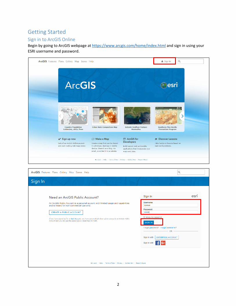
Getting Started Sign in to ArcGIS Online Begin by going to ArcGIS webpage at https://www.arcgis.com/home/index.html and sign in using your ESRI username and password.

3

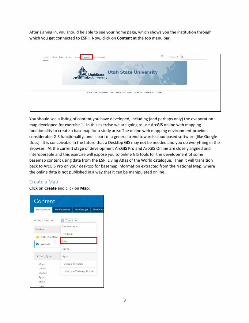
After signing in, you should be able to see your home page, which shows you the institution through which you get connected to ESRI. Now, click on Content at the top menu bar.

You should see a listing of content you have developed, including (and perhaps only) the evaporation map developed for exercise 1. In this exercise we are going to use ArcGIS online web mapping functionality to create a basemap for a study area. The online web mapping environment provides considerable GIS functionality, and is part of a general trend towards cloud based software (like Google Docs). It is conceivable in the future that a Desktop GIS may not be needed and you do everything in the Browser. At the current stage of development ArcGIS Pro and ArcGIS Online are closely aligned and interoperable and this exercise will expose you to online GIS tools for the development of some basemap content using data from the ESRI Living Atlas of the World catalogue. Then it will transition back to ArcGIS Pro on your desktop for basemap information extracted from the National Map, where the online data is not published in a way that it can be manipulated online.

Create a Map Click on Create and click on Map.

4

Now you need to enter a title and some tags for your project. In this exercise, let us name the project Exercise 2 and use GISWR2017 as a tag. Note that after entering the text for the tag, you need to use the tab button so that the tag could be accepted. Then, if you want you can write a summary of this map or leave it blank. You can also organize your online content into folders. In the below, I have used a folder GISWR2017. Click OK to create your map.

The new map should appear as follows:

5

Obtain National Hydrography Data from Living Atlas

Click on Add and choose Browse Living Atlas Layers.

From Browse Living Atlas Layer select the category Water and search on NHDPlus.

Click Close. After adding this layer, your map show the USA National Hydrography Dataset Plus Version 2.1 – Seamless layer.

6

Note that the map automatically zooms in to a resolution where you can see the detail of this dataset. The NHDPlus layer is configured so that it limits the levels at which sublayers are displayed at different scales. If you zoomed out, you will see that most sublayers within NHDPlus dataset will no longer be visible.

Click on the … beneath the layer entry in the table of contents and show item details.

7

This opens a new browser tab that gives metadata on this layer. You should note that this layer holds many key features of the National Hydrography Dataset Plus Version 2.1 including rivers and streams (flowlines) and lakes, bays, and other water bodies (areas and waterbodies) as well as sinks, catchments and watershed boundaries. It is published by ESRI using source data from the USGS and EPA. After learning a bit about this data, go back to your Exercise 2 map tab.

Type San Marcos in the top right search box where it says Find address or place and select San Marcos, TX, USA from among the choices. This should zoom your map to San Marcos.

Click on the map and you will see that the selection identifies HUC12 subwatersheds in this area.

8

Expand the table of contents for USA National Hydrography Dataset Plus Version 2.1 – Seamless and click on the layer name Watershed Boundary Hydrologic Unit 12 to expand tools below it. Click on the table icon (show table) below the name of the layer.

You should see a table at the bottom of the screen.

Note how the layout and behavior of this web map is similar to the layout and behavior of the ArcGIS Pro interface. Many of the concepts and skills you learn working with ArcGIS apply both to web mapping and desktop tools.

You can use the table options button to filter and select features and to center the map on a selected feature or set of features.

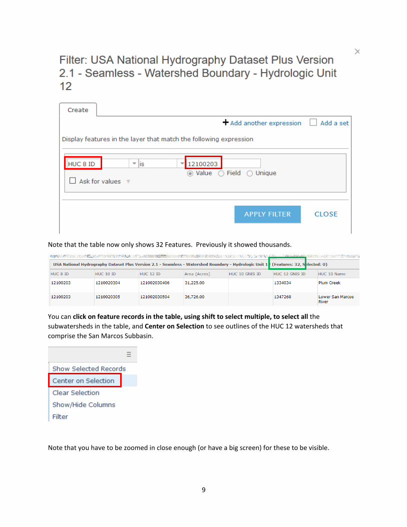
Click on Filter, then in the Create Filter window select HUC 8 ID is 12100203. This is the HUC ID for the San Marcos Subbasin. Click Apply Filter.

9

Note that the table now only shows 32 Features. Previously it showed thousands.

You can click on feature records in the table, using shift to select multiple, to select all the subwatersheds in the table, and Center on Selection to see outlines of the HUC 12 watersheds that comprise the San Marcos Subbasin.

Note that you have to be zoomed in close enough (or have a big screen) for these to be visible.

10

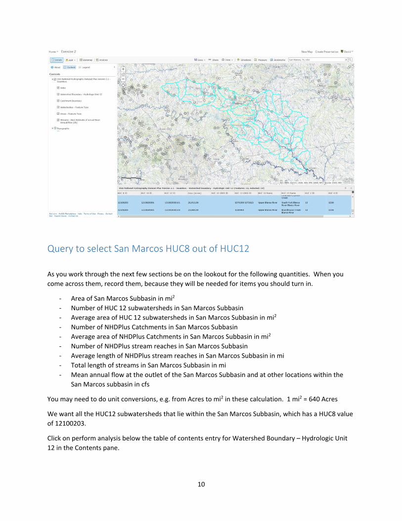
Query to select San Marcos HUC8 out of HUC12

As you work through the next few sections be on the lookout for the following quantities. When you come across them, record them, because they will be needed for items you should turn in.

- Area of San Marcos Subbasin in mi2 - Number of HUC 12 subwatersheds in San Marcos Subbasin - Average area of HUC 12 subwatersheds in San Marcos Subbasin in mi2 - Number of NHDPlus Catchments in San Marcos Subbasin - Average area of NHDPlus Catchments in San Marcos Subbasin in mi2 - Number of NHDPlus stream reaches in San Marcos Subbasin - Average length of NHDPlus stream reaches in San Marcos Subbasin in mi - Total length of streams in San Marcos Subbasin in mi - Mean annual flow at the outlet of the San Marcos Subbasin and at other locations within the

San Marcos subbasin in cfs

You may need to do unit conversions, e.g. from Acres to mi2 in these calculation. 1 mi2 = 640 Acres

We want all the HUC12 subwatersheds that lie within the San Marcos Subbasin, which has a HUC8 value of 12100203.

Click on perform analysis below the table of contents entry for Watershed Boundary – Hydrologic Unit 12 in the Contents pane.

11

This leads you to where you can perform various analyses on the GIS layers. Note that for many online datasets in the Living Atlas and elsewhere the perform analysis button is not enabled. We selected this version of the NHD Plus dataset published by Esri because it does have analysis enabled.

Here, we want to find all the HUC 12 subwatersheds which have a specific HUC 8 ID. To do so, we will implement Find Existing Locations from the Find Location option in the figure above. This selects existing features in our study are that meet a series of criteria we specify.

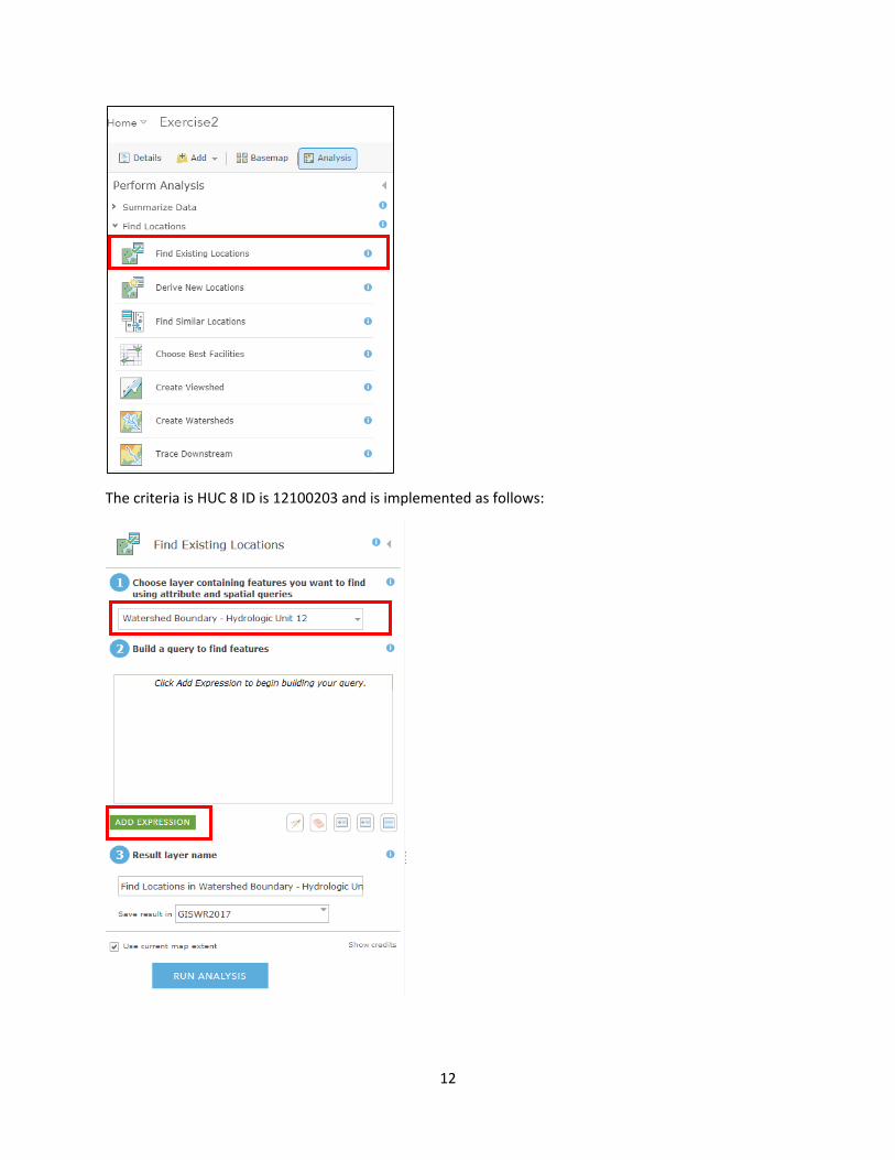
12

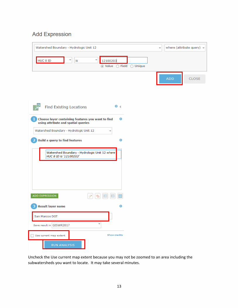
The criteria is HUC 8 ID is 12100203 and is implemented as follows:

13

Uncheck the Use current map extent because you may not be zoomed to an area including the subwatersheds you want to locate. It may take several minutes.

14

For result layer name you need to use a unique name within your organization (The whole of USU or UT Austin). We already used “San Marcos” in testing, so I suggest you each use San Marcos *** where *** is your initials. If you do not do this you may get the error

The result should be as follows:

Open the attribute table for San Marcos layer. Note how many features (HUC 12 subwatersheds there are). Click on the Area heading and calculate statistics. Note the average and sum and use these to fill in some of the information being collected.

15

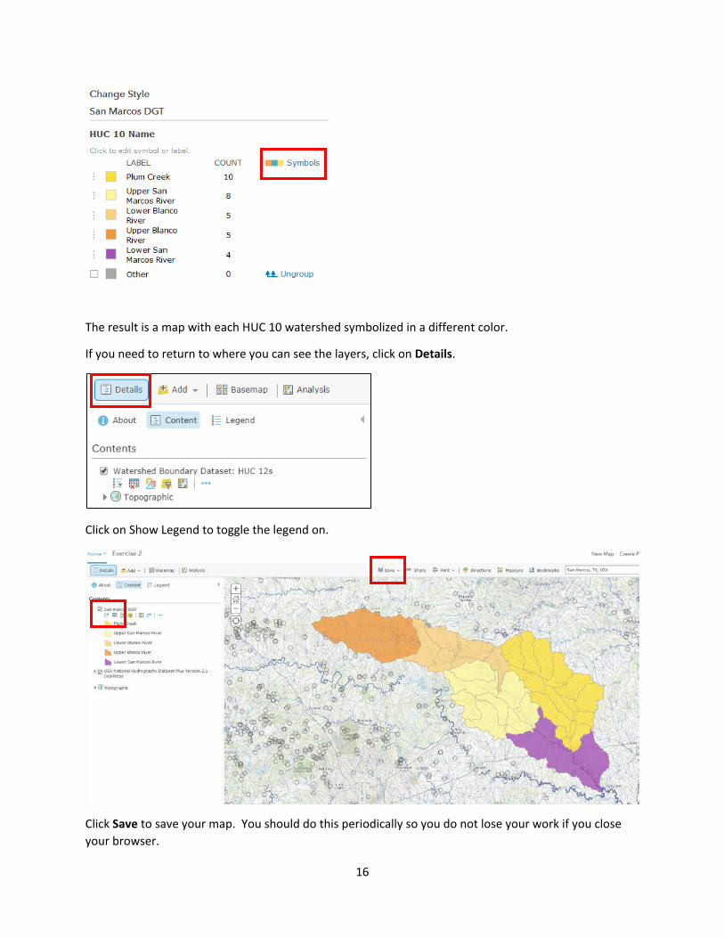
Let’s change the style (symbology) of the layer. Click on the change style button.

Select HUC 10 Name, Options and Symbols to select the colors to use. Click OK and Done

16

The result is a map with each HUC 10 watershed symbolized in a different color.

If you need to return to where you can see the layers, click on Details.

Click on Show Legend to toggle the legend on.

Click Save to save your map. You should do this periodically so you do not lose your work if you close your browser.

17

If you happen to remove the layer from your map you can get it back with the Add button

And filtering on My Content

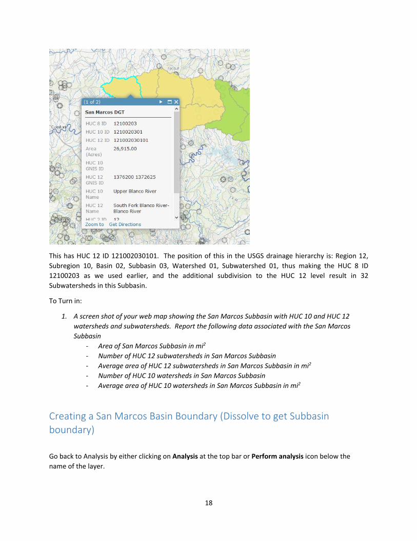
Click on the North-Western subwatershed on the map.

18

This has HUC 12 ID 121002030101. The position of this in the USGS drainage hierarchy is: Region 12, Subregion 10, Basin 02, Subbasin 03, Watershed 01, Subwatershed 01, thus making the HUC 8 ID 12100203 as we used earlier, and the additional subdivision to the HUC 12 level result in 32 Subwatersheds in this Subbasin.

To Turn in:

1. A screen shot of your web map showing the San Marcos Subbasin with HUC 10 and HUC 12 watersheds and subwatersheds. Report the following data associated with the San Marcos Subbasin

- Area of San Marcos Subbasin in mi2 - Number of HUC 12 subwatersheds in San Marcos Subbasin - Average area of HUC 12 subwatersheds in San Marcos Subbasin in mi2 - Number of HUC 10 watersheds in San Marcos Subbasin - Average area of HUC 10 watersheds in San Marcos Subbasin in mi2

Creating a San Marcos Basin Boundary (Dissolve to get Subbasin boundary)

Go back to Analysis by either clicking on Analysis at the top bar or Perform analysis icon below the name of the layer.

19

Click on Manage Data and choose Dissolve Boundaries.

Make sure that in 1 the layer whose boundaries will be dissolved is your San Marcos layer. Keep the default dissolve method and statistic. For Result layer name us a unique name such as SanMarcos Basin Boundary followed by your initials. Uncheck use current map extent and run the analysis.

20

The result should be a single polygon for the San Marcos Subbasin.

21

Adjust the Style (symbology) to transparent fill with solid green basin outline

22

Save your map.

Obtaining the San Marcos Flowlines and Catchments

Now, let’s extract flowlines and catchments from the USA National Hydrography Dataset Plus Version 2.1 – Seamless layer that we added earlier. This NHDPlus dataset includes Catchment Boundaries and Streams.

23

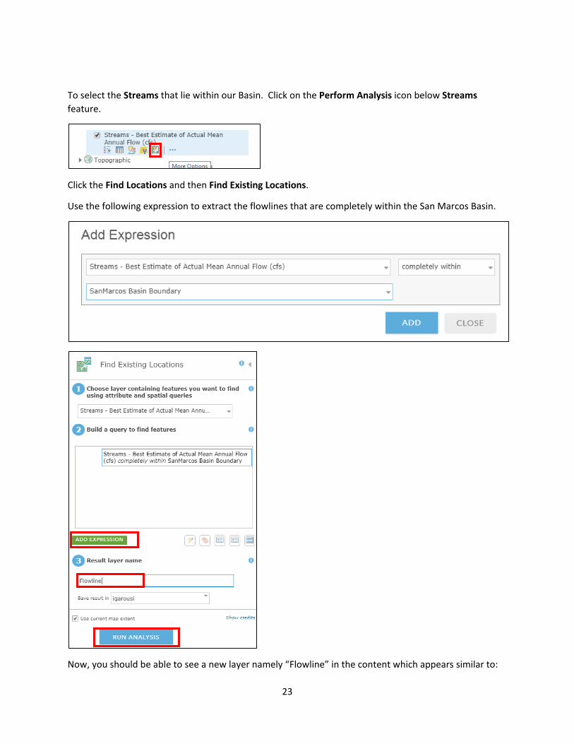
To select the Streams that lie within our Basin. Click on the Perform Analysis icon below Streams feature.

Click the Find Locations and then Find Existing Locations.

Use the following expression to extract the flowlines that are completely within the San Marcos Basin.

Now, you should be able to see a new layer namely “Flowline” in the content which appears similar to:

24

For extracting the catchments, click on perform analysis icon below the Catchment Boundary.

From Find Existing Locations, use the following expression that selects all catchments that intersect with the flowlines.

25

The result should be as follows. You may need to change the style and layer ordering to see the information more clearly.

Note that there is a 1:1 relationship between Flowlines and catchments. The flowline Common Identifier (COMID) matches with Catchment Feature ID. It is this connectivity that allows runoff generated from catchments to be linked to stream reaches (flowlines) in the National Water Model.

In this map the streams all look alike, so let’s recolor the Flowline according to the Best Estimate of Actual Mean Flow attribute. Click on the Change Style icon below Flowline layer.

26

Select the following:

After selecting “Counts and Amounts (Size)”, click on OPTIONS. You can change the symbol to blue color. Also, you can define the minimum and maximum size of the line thickness, which is based on the value of mean flow. Streams with higher values of flow are thicker. Check Classify Data to control the precise classes associated with different line thicknesses. Click OK and the DONE.

27

Turn on the legend in the contents to get a nice display of the streams symbolized using line width based on actual mean flow.

28

Search for Wimberley at the top right side of the map in the ArcGIS Online.

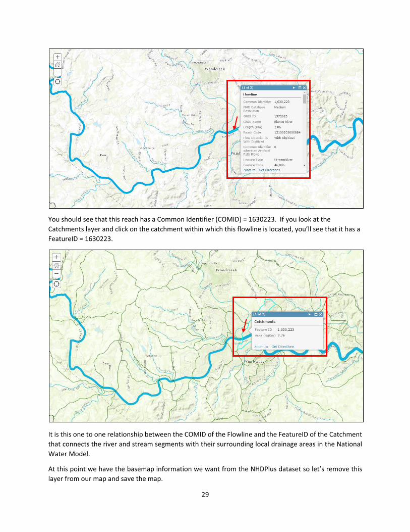
Click on the reach of the Blanco River just downstream of Wimberley.

29

You should see that this reach has a Common Identifier (COMID) = 1630223. If you look at the Catchments layer and click on the catchment within which this flowline is located, you’ll see that it has a FeatureID = 1630223.

It is this one to one relationship between the COMID of the Flowline and the FeatureID of the Catchment that connects the river and stream segments with their surrounding local drainage areas in the National Water Model.

At this point we have the basemap information we want from the NHDPlus dataset so let’s remove this layer from our map and save the map.

30

Click Save at the top of your map.

Use the attribute tables associated with Flowline and Catchments, and the Statistics calculator on attribute table fields to determine the number and average area of Catchments, and number and average and total length of flowlines. Identify the most downstream reach in the San Marcos Subbasin and determine the best estimate of actual mean flow. Also note the Total upstream catchment area from downstream end of Flowline.

To Turn in:

2. A screenshot of your web map showing Flowlines symbolized with mean flow, Catchments and San Marcos Basin Boundary. Show legend information for the Flowlines. Report the following data associated with the San Marcos Subbasin Flowlines and Catchments

- Total Area of San Marcos Subbasin determined from summing Catchment areas as well as from the most downstream flowline in mi2. Comment on any differences and any differences with the area reported in #1 above.

- Number of NHDPlus Catchments in San Marcos Subbasin - Average area of NHDPlus Catchments in San Marcos Subbasin in mi2 - Number of NHDPlus flowlines in San Marcos Subbasin - Average length of NHDPlus flowlines in San Marcos Subbasin in mi - Total length of NHDPlus flowlines in San Marcos Subbasin in mi - Best estimate of actual mean flow at the outlet of the San Marcos Subbasin in cfs. - Common Identifier (COMID) of the Flowline at the outlet of the San Marcos Subbasin

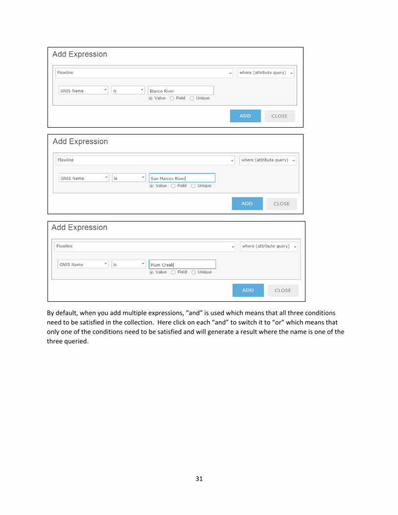
Extracting Main Rivers There are three main rivers in the San Marcos Subbasin. These are the Blanco River, San Marcos River and Plum Creek. Let’s create a Main Rivers layer. To do so, click on perform analysis below the Flowline layer and then select Find Existing Locations. Define three expressions to query for GNIS Name to be “Blanco River” or “San Marcos River” or “Plum Creek”.

31

By default, when you add multiple expressions, “and” is used which means that all three conditions need to be satisfied in the collection. Here click on each “and” to switch it to “or” which means that only one of the conditions need to be satisfied and will generate a result where the name is one of the three queried.

32

The result is:

33

Change the symbology so that each river is shown with a different color. Click on Change style icon below the new layer.

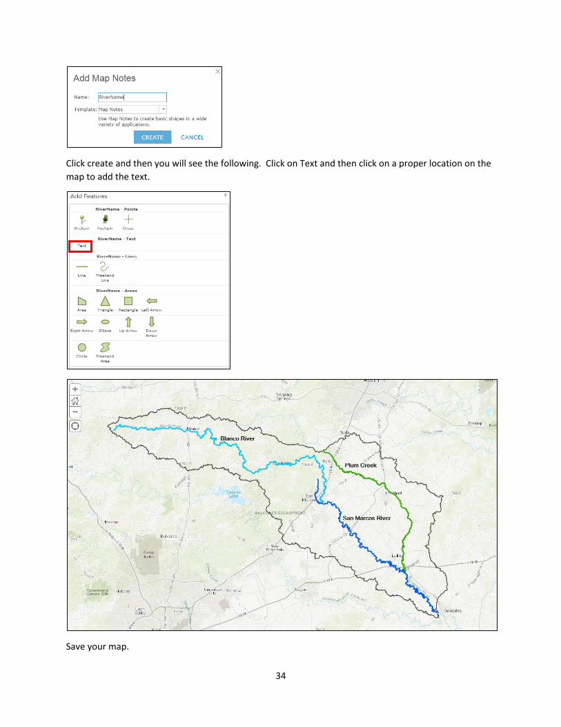
Now let’s add Map Notes to label each river. From “Add”, select “Add Map Notes”.

34

Click create and then you will see the following. Click on Text and then click on a proper location on the map to add the text.

Save your map.

35

To Turn in:

3. A screen shot of your web map showing the three main rivers with labels in the San Marcos Subbasin

Creating a Point Feature Class of Stream Gauges

Now you are going to build a new Feature Class yourself of stream gage locations in the San Marcos basin. I have extracted information from the USGS site information at http://waterdata.usgs.gov/tx/nwis/si

SiteID SiteName Latitude Longitude DASqMile MAFlow

(cfs)

08171000 Blanco Rv at Wimberley, Tx 29⁰ 59' 39" 98⁰ 05' 19" 355 142

08171300 Blanco Rv nr Kyle, Tx 29⁰ 58' 45" 97⁰ 54' 35" 412 165

08172400 Plum Ck at Lockhart, Tx 29⁰ 55' 22" 97⁰ 40' 44" 112 49

08173000 Plum Ck nr Luling, Tx 29⁰ 41' 58" 97⁰ 36' 12" 309 114

08172000 San Marcos Rv at Luling, Tx 29⁰ 39' 58" 97⁰ 39' 02" 838 408

08170500 San Marcos Rv at San Marcos, Tx 29⁰ 53' 20" 97⁰ 56' 02" 48.9 176

Using Excel develop a table containing SiteID, Latitude (as lat) and Longitude (as long) coordinates of the gauges. Save this in a file named latlong.csv. You will need to evaluate decimal degrees from the degree, minute and second information.

In your Exercise 2 web map on ArcGIS Online select Add button and choose “Add Layer from File”. Navigate to your latlong.csv file and import it.

36

Note that when you add a CSV file with location information (street addresses or latitude-longitude coordinates), the features can be located on the map. If you add a CSV file that doesn't contain location information, a table is added instead. In this case, the file contains latitude-longitude coordinates. Use the Add CSV Layer window to set LatDD and LongDD as Latitude and Longitude fields and click Add Layer

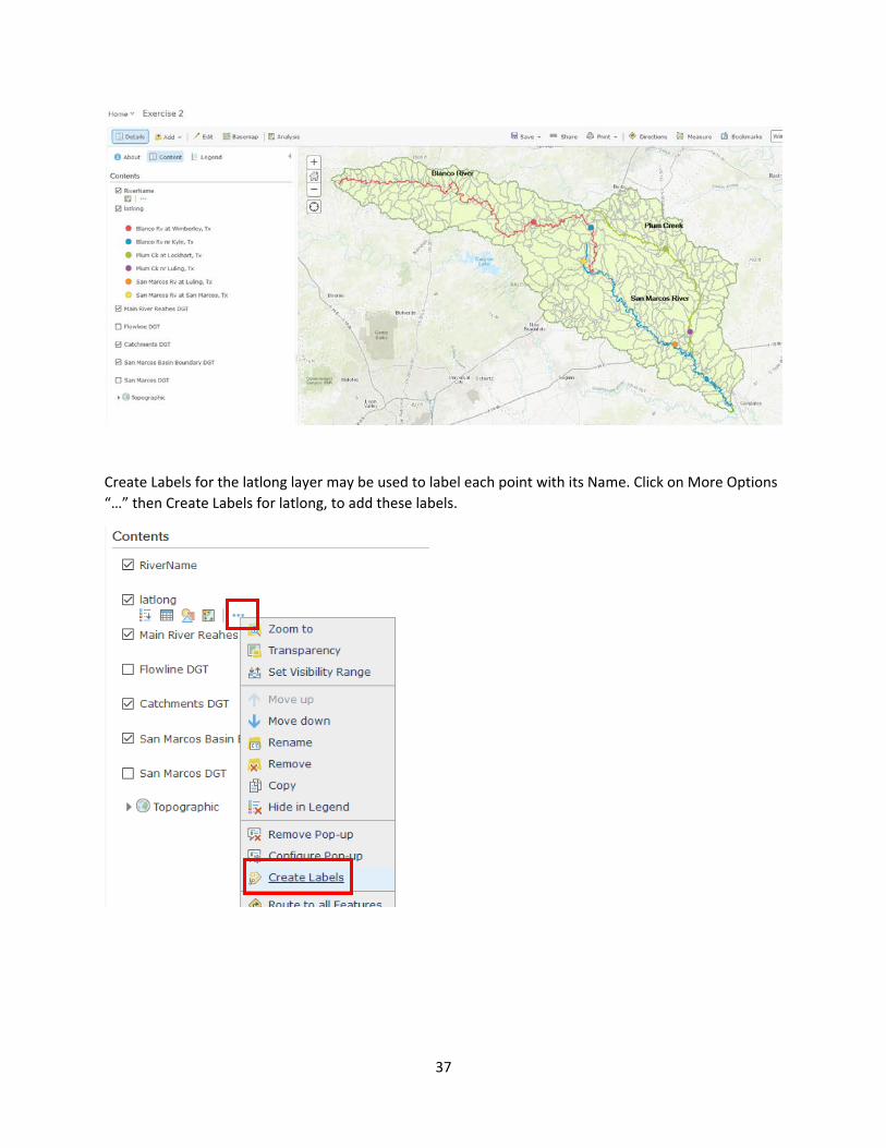
The system then gives you the option to adjust symbology. Here I used unique symbols based on Site Name.

37

Create Labels for the latlong layer may be used to label each point with its Name. Click on More Options “…” then Create Labels for latlong, to add these labels.

38

Save your map.

Zoom in on each stream gauge and identify the nearest NHDPlus flowline and record its best estimate of actual mean flow (cfs) Fill out the following table. Note that NHDPlus area values are in km2 so you will need to do km to mi conversions. 1 mi = 1.60934 km. 1 mi2 = 2.59 km2

Site ID Site Name Drainage Area (mi2)

MAFlow (cfs)

NHDPlus Reach COMID for reach nearest to the stream gauge

NHDPlus best estimate of actual mean flow (cfs)

NHDPlus Total upstream catchment area from downstream end of Flowline (mi2)

08171000 Blanco Rv at Wimberley, Tx

355 142

08171300 Blanco Rv nr Kyle, Tx

412 165

08172400 Plum Ck at Lockhart, Tx

112 49

08173000 Plum Ck nr Luling, Tx

309 114

08172000 San Marcos Rv at Luling, Tx

838 408

08170500 San Marcos Rv at San Marcos, Tx

48.9 176

39

Comment on any differences that seem out of the ordinary or larger than common uncertainty or numerical calculation accuracy.

To turn in

4. A screen shot of your web map showing the labeled stream gauges and the table above with quantities filled in and interpretive comments on differences.

We are done with the web map, so close the browser with Exercise 2 map.

Land Cover Information for the San Marcos Basin

Up to this point the necessary data has all been obtained from the Living Atlas using ArcGIS online mapping functionality. Online functionality for working with raster data is limited, so here we will switch to ArcGIS Pro on the desktop and add to our base map raster Land Cover data downloaded from the National Map.

Open ArcGIS Pro and create a Blank project.

I used the name Ex2 Desktop so I can tell which project is from the desktop and which from the web.

Under Portal My Content locate your Exercise 2 Web Map and Right Click to Add and Open. Note that this should be with the Catalog View active, not while you are looking at a map, so be sure you start from a blank project, not a map project.

40

You should see that ArcGIS Pro opens with a replica of your web map in the Desktop Software. Pretty Slick! This is an example of the interoperability between web and desktop software.

Let’s obtain Land Cover Information from the National Map. Go to https://viewer.nationalmap.gov/launch/

Click on Download GIS Data in the GIS Data box.

In the Search location box enter San Marcos and from the choices pick San Marcos, Texas.

41

The Map should zoom to San Marcos. With the Use Map check box set this serves to focus the search in the map area. Now in the panel on the left select National Land Cover Database and State, then click on Find Products

Three products should be shown in the left side. Click on Download for the NLCD 2011 Land Cover option.

42

Unzip the file downloaded into a convenient location. Locate the file NLCD2011_LC_Texas.tif and load this into your ArcGIS Pro Map. (You may need to attach the folder to find it). I loaded the file by dragging from the Catalog pane. Zoom to the extent of the layer to see that you have Landcover data for the whole of Texas.

43

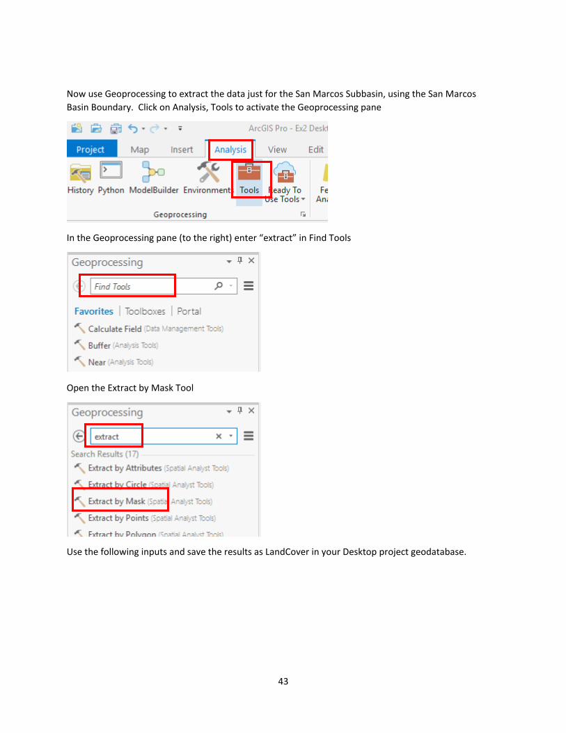
Now use Geoprocessing to extract the data just for the San Marcos Subbasin, using the San Marcos Basin Boundary. Click on Analysis, Tools to activate the Geoprocessing pane

In the Geoprocessing pane (to the right) enter “extract” in Find Tools

Open the Extract by Mask Tool

Use the following inputs and save the results as LandCover in your Desktop project geodatabase.

44

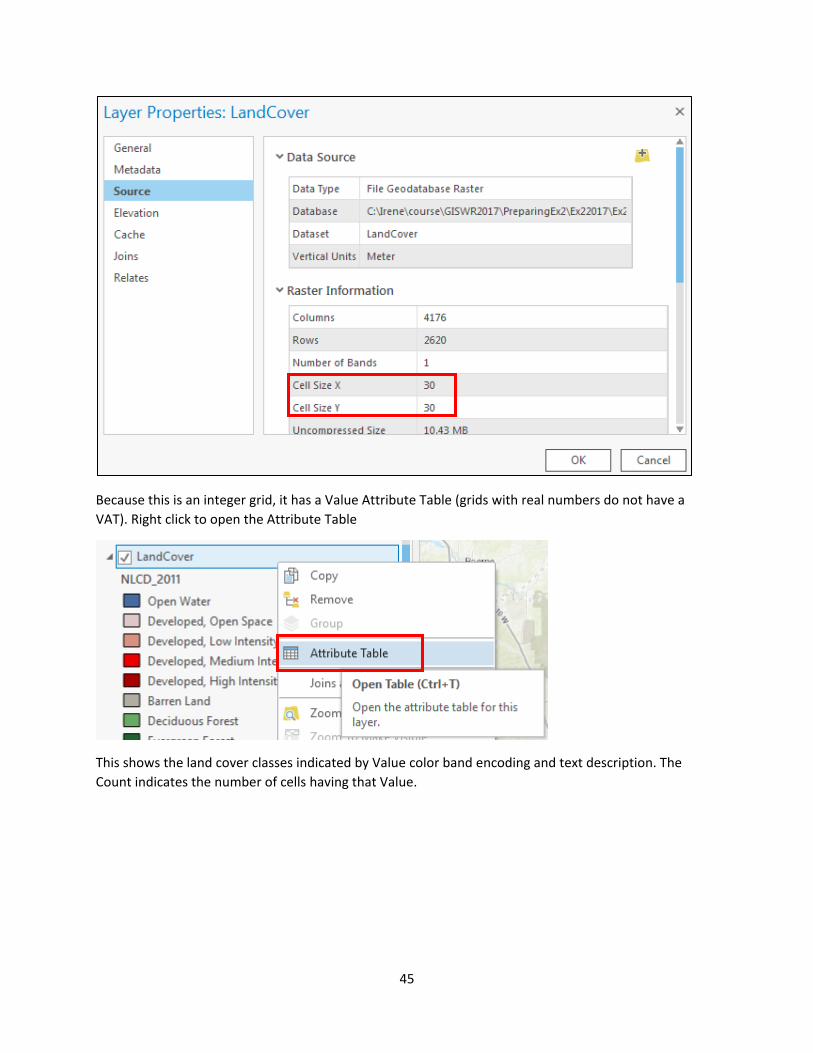
If you right click on the LandCover raster and open its properties, and then select Raster Information, you’ll see it is a raster with 30m X 30m cells (these are derived from 30m Landsat imagery).

45

Because this is an integer grid, it has a Value Attribute Table (grids with real numbers do not have a VAT). Right click to open the Attribute Table

This shows the land cover classes indicated by Value color band encoding and text description. The Count indicates the number of cells having that Value.

46

Suppose, for the purposes of simplification we are interested in aggregating the landcover into fewer classes

1. Water and Wetlands (11,90,95) 2. Developed (21-24) 3. Forest (41-43) 4. Agriculture (71-82) 5. Shrub and Barren (31 and 52)

This requires reclassifying the LandCover raster. In Geoprocessing search for reclassify and then choose Reclassify (Spatial Analyst Tools).

47

Set the inputs as follows and Run.

48

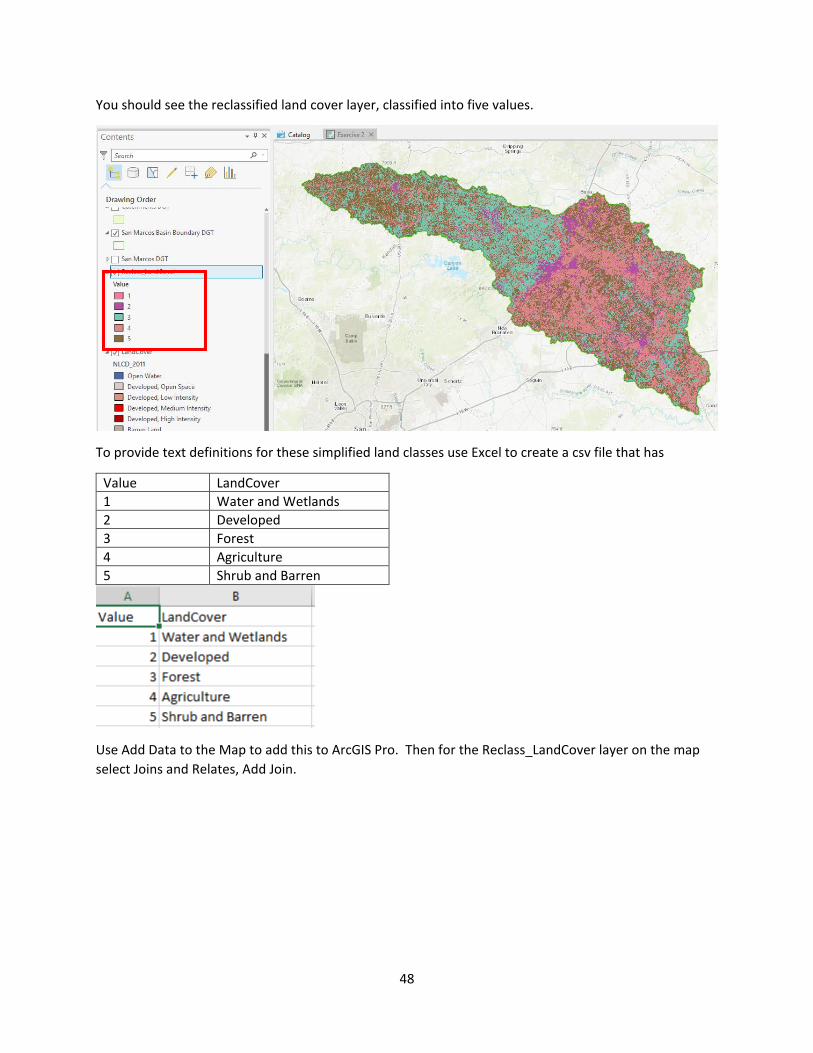
You should see the reclassified land cover layer, classified into five values.

To provide text definitions for these simplified land classes use Excel to create a csv file that has

Value LandCover 1 Water and Wetlands 2 Developed 3 Forest 4 Agriculture 5 Shrub and Barren

Use Add Data to the Map to add this to ArcGIS Pro. Then for the Reclass_LandCover layer on the map select Joins and Relates, Add Join.

49

In the Geoprocessing pane set the Add Join Parameters as follows and click Run

If you open the attribute table for Reclas_LandCover you should see:

50

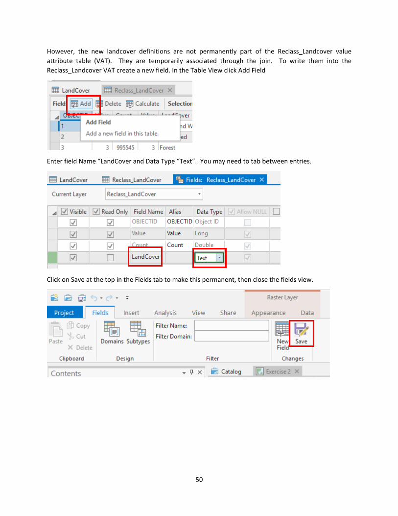
However, the new landcover definitions are not permanently part of the Reclass_Landcover value attribute table (VAT). They are temporarily associated through the join. To write them into the Reclass_Landcover VAT create a new field. In the Table View click Add Field

Enter field Name “LandCover and Data Type “Text”. You may need to tab between entries.

Click on Save at the top in the Fields tab to make this permanent, then close the fields view.

51

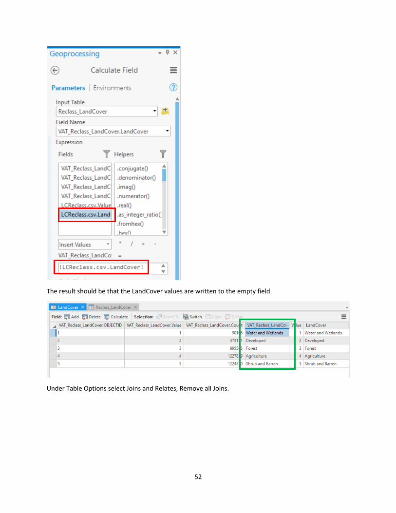
Notice that in the Reclass_LandCover table there is an empty field LandCover and that all field names have been preceded by their table name to disambiguate. The field is thus VAT_Reclass_LandCover.LandCover.

Right click on this Field and select Calculate Field

In the Geoprocessing pane the Calculate Field tool opens. Double click on LCReclass.csv.LandCover in Fields so that it appears in the box below =. Then click Run.

52

The result should be that the LandCover values are written to the empty field.

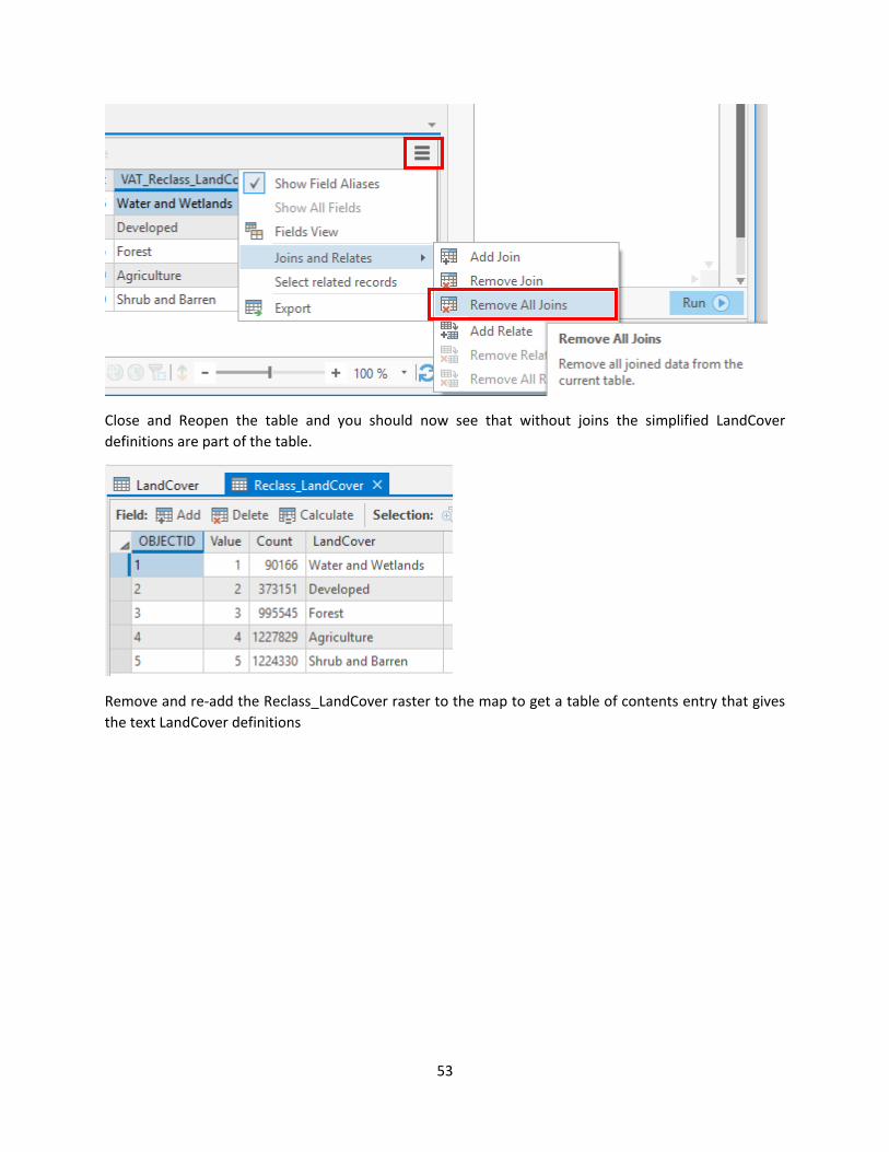
Under Table Options select Joins and Relates, Remove all Joins.

53

Close and Reopen the table and you should now see that without joins the simplified LandCover definitions are part of the table.

Remove and re-add the Reclass_LandCover raster to the map to get a table of contents entry that gives the text LandCover definitions

54

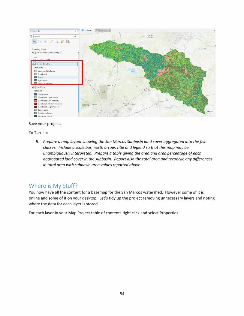
Save your project.

To Turn in:

5. Prepare a map layout showing the San Marcos Subbasin land cover aggregated into the five classes. Include a scale bar, north arrow, title and legend so that this map may be unambiguously interpreted. Prepare a table giving the area and area percentage of each aggregated land cover in the subbasin. Report also the total area and reconcile any differences in total area with subbasin area values reported above.

Where is My Stuff? You now have all the content for a basemap for the San Marcos watershed. However some of it is online and some of it on your desktop. Let’s tidy up the project removing unnecessary layers and noting where the data for each layer is stored.

For each layer in your Map Project table of contents right click and select Properties

55

In the Layer Properties window click on Source and note the Location of the Data. For example for the RiverName layer, the layer of labels with River Names we see that this is in the Desktop database, even though it was created online.

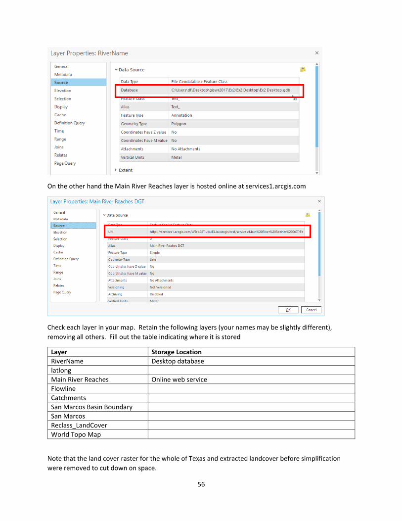
56

On the other hand the Main River Reaches layer is hosted online at services1.arcgis.com

Check each layer in your map. Retain the following layers (your names may be slightly different), removing all others. Fill out the table indicating where it is stored

Layer Storage Location RiverName Desktop database latlong Main River Reaches Online web service Flowline Catchments San Marcos Basin Boundary San Marcos Reclass_LandCover World Topo Map

Note that the land cover raster for the whole of Texas and extracted landcover before simplification were removed to cut down on space.

57

Once you have removed layers not in the list above, save your project.

To Turn in:

6. The table above reporting the location of each layer in your San Marcos Subbasin basemap.

Summary of items to be turned in 1. A screen shot of your web map showing the San Marcos Subbasin with HUC 10 and HUC 12

watersheds and subwatersheds. Report the following data associated with the San Marcos Subbasin

- Area of San Marcos Subbasin in mi2 - Number of HUC 12 subwatersheds in San Marcos Subbasin - Average area of HUC 12 subwatersheds in San Marcos Subbasin in mi2 - Number of HUC 10 watersheds in San Marcos Subbasin - Average area of HUC 10 watersheds in San Marcos Subbasin in mi2

2. A screenshot of your web map showing Flowlines symbolized with mean flow, Catchments and

San Marcos Basin Boundary. Show legend information for the Flowlines. Report the following data associated with the San Marcos Subbasin Flowlines and Catchments

- Total Area of San Marcos Subbasin determined from summing Catchment areas as well as from the most downstream flowline in mi2. Comment on any differences and any differences with the area reported in #1 above.

- Number of NHDPlus Catchments in San Marcos Subbasin - Average area of NHDPlus Catchments in San Marcos Subbasin in mi2 - Number of NHDPlus flowlines in San Marcos Subbasin - Average length of NHDPlus flowlines in San Marcos Subbasin in mi - Total length of NHDPlus flowlines in San Marcos Subbasin in mi - Best estimate of actual mean flow at the outlet of the San Marcos Subbasin in cfs. - Common Identifier (COMID) of the Flowline at the outlet of the San Marcos Subbasin

3. A screen shot of your web map showing the three main rivers with labels in the San Marcos

Subbasin

4. A screen shot of your web map showing the labeled stream gauges and the table above with quantities filled in and interpretive comments on differences.

5. Prepare a map layout showing the San Marcos Subbasin land cover aggregated into the five classes. Include a scale bar, north arrow, title and legend so that this map may be unambiguously interpreted. Prepare a table giving the area and area percentage of each aggregated land cover in the subbasin. Report also the total area and reconcile any differences in total area with subbasin area values reported above.

6. The table above reporting the location of each layer in your San Marcos Subbasin basemap.