Exercise 1a: Stress and displacement analysis in a simply supported beam. In this exercise, a structural analysis is performed on a simple supported beam. The structural model with loads and constraints applied are shown in the figure below. The objective is to create a finite element model that is good enough to predict the theoretical solution for this model. To download the model, please click HERE.

FEA model

Model Information o Force = 1000 N (Applied in a segment equivalent to 2mm)

o Beam properties: L = 1000, B = 10 and H = 20 mm

o Material Steel: E =210000 MPa and Nu=0.3

o UNITS: N, mm, ton, s

Theoretical Results

MPaBHFL

IcM

HB

HLF

37523*

212*

24*

maxmax 3 ====σ

mmEBHFL

EFL

EIFLU

BH881.14

44848 3

3

12

33

max 3 =−=−=−=

Problem Setup Copy the file: Beam_shell_geometry.hm

12345 23

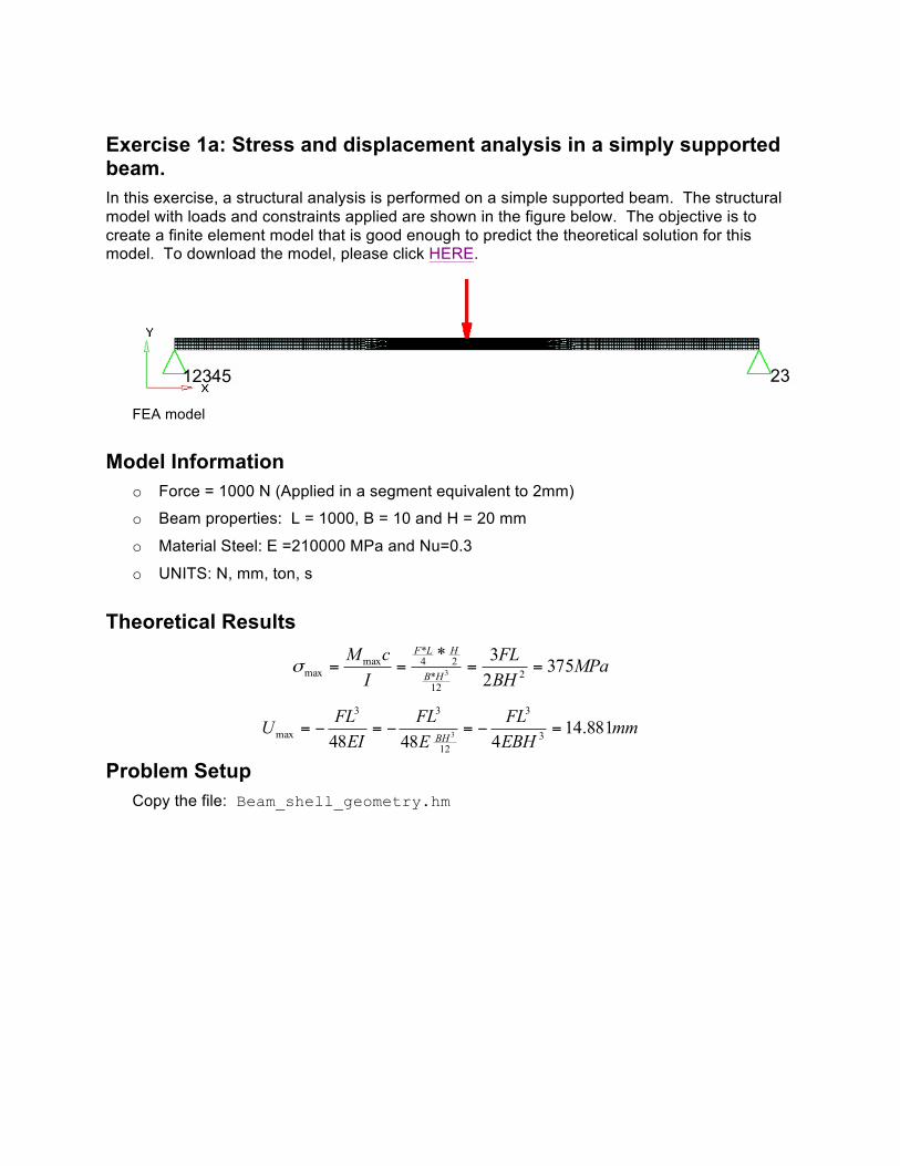
Step 1: Launch HyperMesh Desktop and Set the User Profile 1. Launch HyperMesh Desktop.

The User Profiles dialog will appear by default.

2. Choose OptiStruct as the user profile by selecting the radio button beside it.

3. Click OK.

Step 2: Open the HyperMesh Desktop database model This HM database only contains geometry information.

1. From the pull down menu select File > Open > Model. An Open File pop up window appears to select the HyperMesh database.

2. Browse in the training directory for a file named Beam_shell_geometry.hm and click Open.

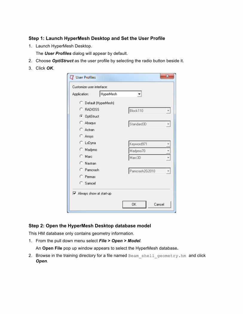
Step 3: Define the Material 1. Right-click on the Model Browser tab and select Create > Material. 2. The new material card opens in the Entity Editor. Enter the following values for the card.

Here we will use MAT1 which is a linear isotropic material that can represent the steel behavior well. For more details about this material or other material formulations, please refer to the online help.

Step 4: Create Model Properties 1. Right-click on the Model Browser to Create > Property to create a new property card,

which opens in the Entity Editor. 2. Enter the following values to define the Beam property card.

Step 5: Assign the property to the component 1. In the Model Browser, expand the Component section and right-click on the component

beam to select Assign.

2. In the dialog box, select the property Beam.

3. Click OK.

This will make that all elements in this component use this property. If an element from this component has another property associated with itself directly, this property will be preserved, i.e. HyperMesh will ignore the component property for this element.

Step 6: Create the finite element mesh 1. From the pull down menu, click on Mesh > Create > 2D Automesh.

2. Click on surfs and choose all to select all surfaces.

3. Verify that the element size is set to 10 and the mesh type is set to mixed. Then click mesh.

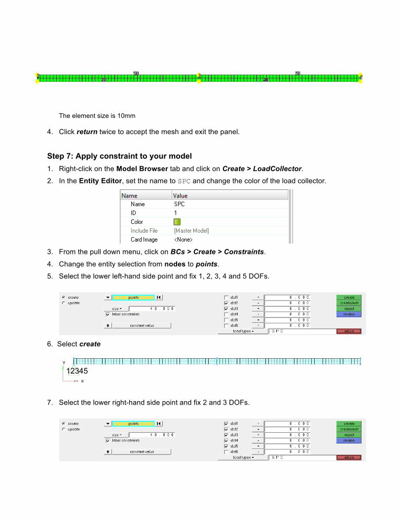
The element size is 10mm

4. Click return twice to accept the mesh and exit the panel.

Step 7: Apply constraint to your model 1. Right-click on the Model Browser tab and click on Create > LoadCollector. 2. In the Entity Editor, set the name to SPC and change the color of the load collector.

3. From the pull down menu, click on BCs > Create > Constraints.

4. Change the entity selection from nodes to points.

5. Select the lower left-hand side point and fix 1, 2, 3, 4 and 5 DOFs.

6. Select create

7. Select the lower right-hand side point and fix 2 and 3 DOFs.

12345

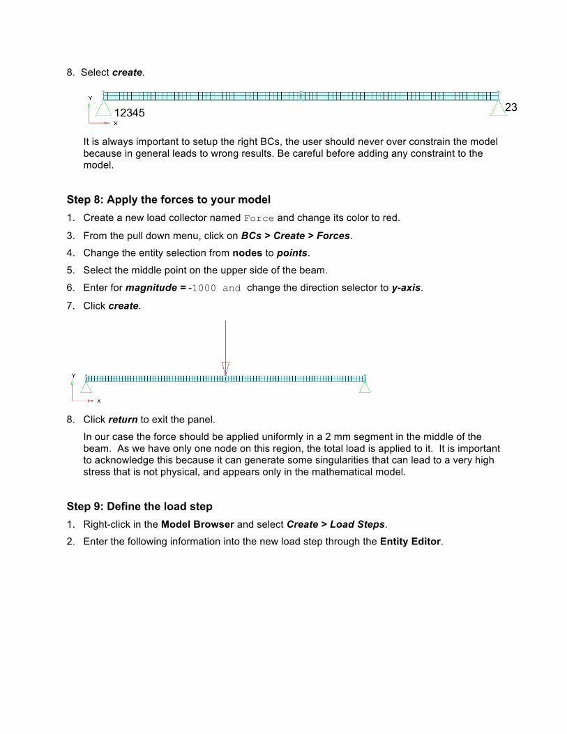
8. Select create.

It is always important to setup the right BCs, the user should never over constrain the model because in general leads to wrong results. Be careful before adding any constraint to the model.

Step 8: Apply the forces to your model 1. Create a new load collector named Force and change its color to red.

3. From the pull down menu, click on BCs > Create > Forces.

4. Change the entity selection from nodes to points.

5. Select the middle point on the upper side of the beam.

6. Enter for magnitude = -1000 and change the direction selector to y-axis.

7. Click create.

8. Click return to exit the panel.

In our case the force should be applied uniformly in a 2 mm segment in the middle of the beam. As we have only one node on this region, the total load is applied to it. It is important to acknowledge this because it can generate some singularities that can lead to a very high stress that is not physical, and appears only in the mathematical model.

Step 9: Define the load step 1. Right-click in the Model Browser and select Create > Load Steps.

2. Enter the following information into the new load step through the Entity Editor.

12345 23

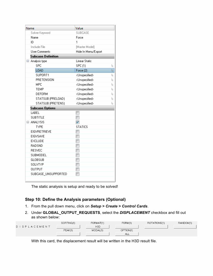
The static analysis is setup and ready to be solved!

Step 10: Define the Analysis parameters (Optional) 1. From the pull down menu, click on Setup > Create > Control Cards.

2. Under GLOBAL_OUTPUT_REQUESTS, select the DISPLACEMENT checkbox and fill out as shown below:

With this card, the displacement result will be written in the H3D result file.

3. Under GLOBAL_OUTPUT_REQUESTS, select the STRESS and fill out the card as shown below:

4. Click return to exit the GLOBAL_OUTPUT_REQUEST page.

4. Look for the control card SCREEN and fill out, as shown below:

OptiStruct will show on the screen what it is writing in the .out file.

5. Look for the card PARAM panel and setup AUTOSPC NO, as shown below:

By default, OptiStruct uses AUTOSPC, ON as it helps to prevent undesired stops or failure runs. For example, if the model has an element unattached to the structure with no constraint applied to it, the run would stop complaining about a rigid body movement. With AUTOSPC ON, OptiStruct would automatically fix this element and run the analysis.

The user should be aware of any DOF fixed by the AUTOSPC. As we discussed before, it can lead to a wrong behavior. Also, do not forget that in the end, if the run is made with “AUTOSPC ON”, to verify which DOF was fixed and if this has not affected the solution.

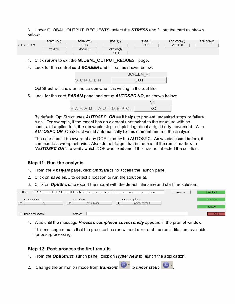
Step 11: Run the analysis 1. From the Analysis page, click OptiStruct to access the launch panel.

2. Click on save as… to select a location to run the solution at.

3. Click on OptiStruct to export the model with the default filename and start the solution.

4. Wait until the message Process completed successfully appears in the prompt window.

This message means that the process has run without error and the result files are available for post-processing.

Step 12: Post-process the first results 1. From the OptiStruct launch panel, click on HyperView to launch the application.

2. Change the animation mode from transient to linear static .

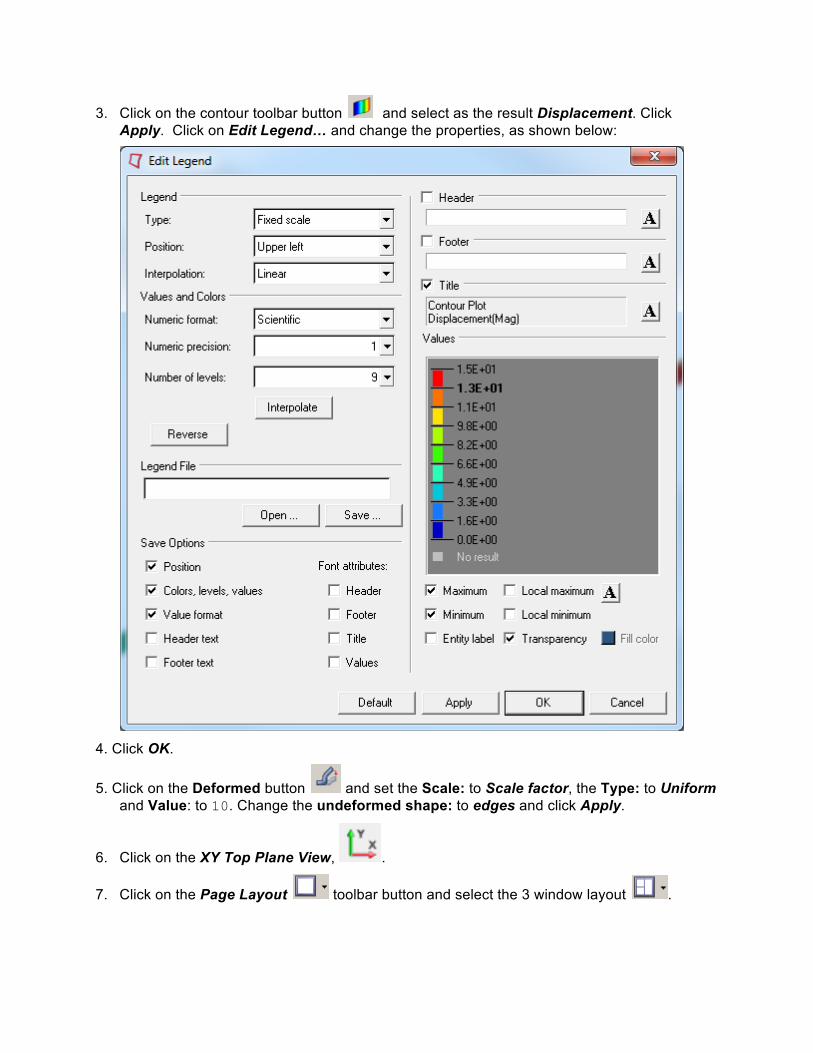
3. Click on the contour toolbar button and select as the result Displacement. Click Apply. Click on Edit Legend… and change the properties, as shown below:

4. Click OK.

5. Click on the Deformed button and set the Scale: to Scale factor, the Type: to Uniform and Value: to 10. Change the undeformed shape: to edges and click Apply.

6. Click on the XY Top Plane View, .

7. Click on the Page Layout toolbar button and select the 3 window layout .

8. Click on the Note toolbar button and change the actual text in the Description: to BEAM MODEL and click Apply. From the pull-down menu, click Edit > Copy > Window and click on the second window, then click Edit > Paste > Window. Repeat this procedure for the third window.

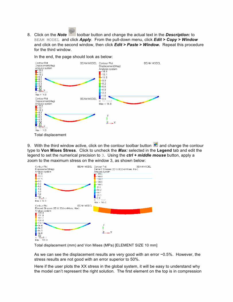
In the end, the page should look as below:

Total displacement

9. With the third window active, click on the contour toolbar button and change the contour type to Von Mises Stress. Click to uncheck the Max: selected in the Legend tab and edit the legend to set the numerical precision to 3. Using the ctrl + middle mouse button, apply a zoom to the maximum stress on the window 3, as shown below:

Total displacement (mm) and Von Mises (MPa) [ELEMENT SIZE 10 mm]

As we can see the displacement results are very good with an error ~0.5%. However, the stress results are not good with an error superior to 50%.

Here if the user plots the XX stress in the global system, it will be easy to understand why the model can’t represent the right solution. The first element on the top is in compression

and the bottom element is tension. This means that there is a BIG STEP between it that is not captured with this coarse mesh. To improve it, the user will need to refine the mesh.

Step 13: Refinement study (Optional Elem = 5 mm) The next steps are used to determine a good mesh to solve this problem and it can be set aside if the user has a good background in FEA analysis.

1. Now coming back to HyperMesh Desktop, click return to close the OptiStruct launch panel.

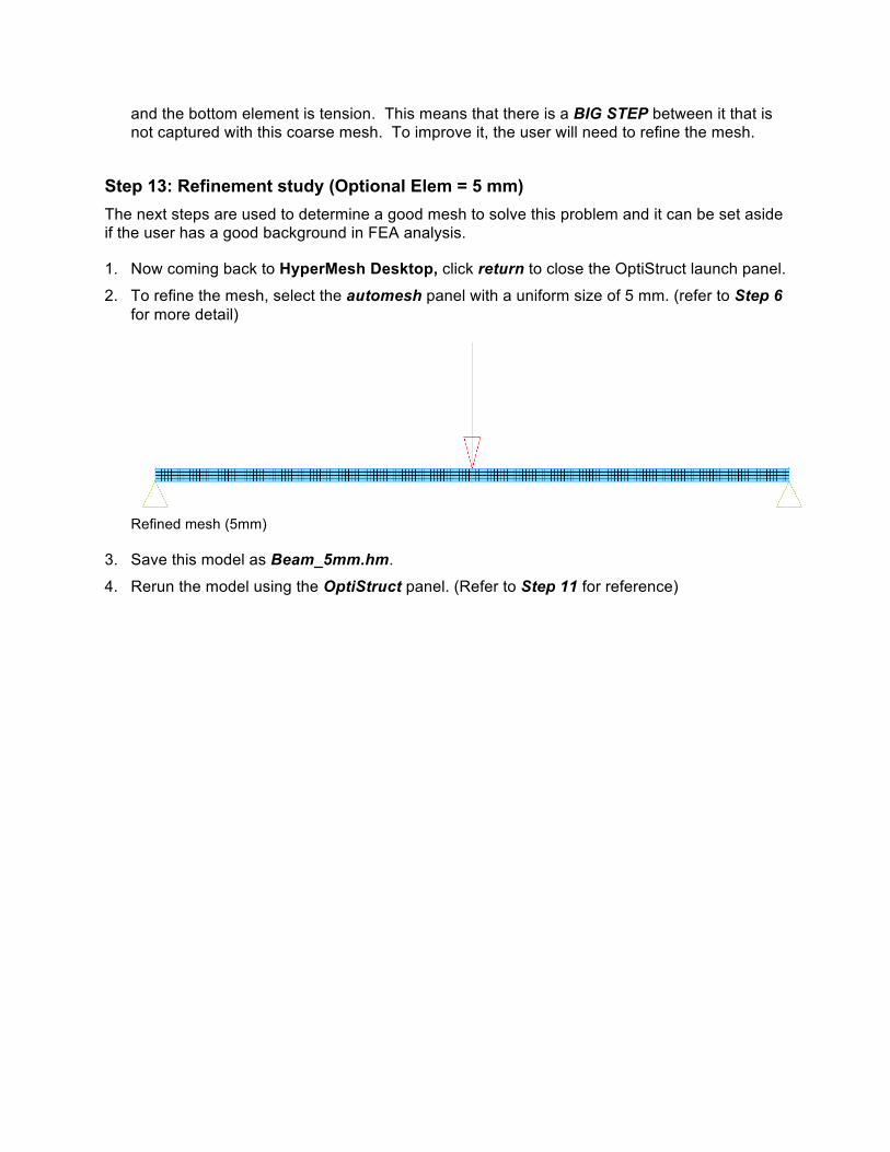
2. To refine the mesh, select the automesh panel with a uniform size of 5 mm. (refer to Step 6 for more detail)

Refined mesh (5mm)

3. Save this model as Beam_5mm.hm.

4. Rerun the model using the OptiStruct panel. (Refer to Step 11 for reference)

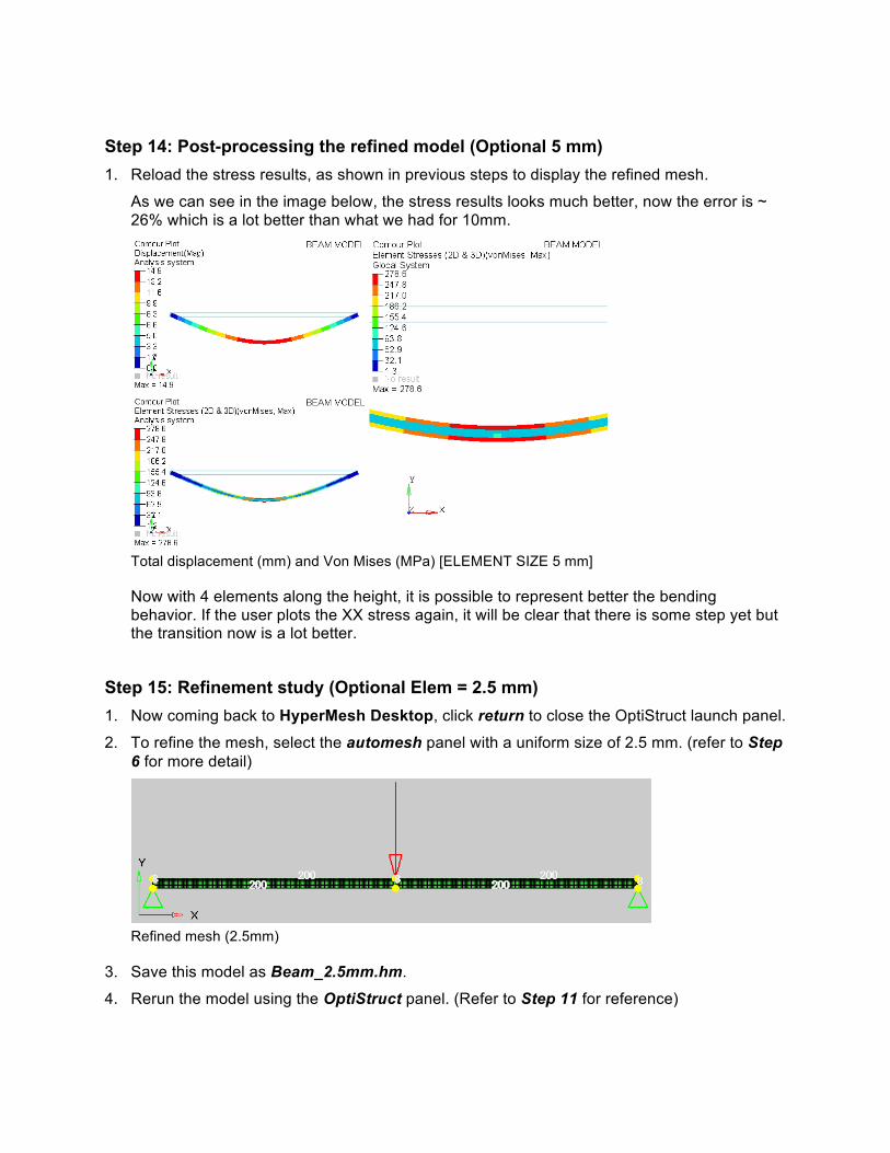
Step 14: Post-processing the refined model (Optional 5 mm) 1. Reload the stress results, as shown in previous steps to display the refined mesh.

As we can see in the image below, the stress results looks much better, now the error is ~ 26% which is a lot better than what we had for 10mm.

Total displacement (mm) and Von Mises (MPa) [ELEMENT SIZE 5 mm]

Now with 4 elements along the height, it is possible to represent better the bending behavior. If the user plots the XX stress again, it will be clear that there is some step yet but the transition now is a lot better.

Step 15: Refinement study (Optional Elem = 2.5 mm) 1. Now coming back to HyperMesh Desktop, click return to close the OptiStruct launch panel.

2. To refine the mesh, select the automesh panel with a uniform size of 2.5 mm. (refer to Step 6 for more detail)

Refined mesh (2.5mm)

3. Save this model as Beam_2.5mm.hm.

4. Rerun the model using the OptiStruct panel. (Refer to Step 11 for reference)

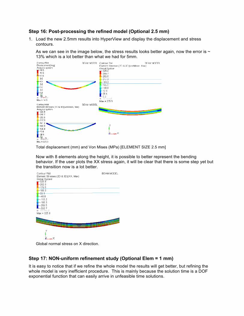
Step 16: Post-processing the refined model (Optional 2.5 mm) 1. Load the new 2.5mm results into HyperView and display the displacement and stress

contours.

As we can see in the image below, the stress results looks better again, now the error is ~ 13% which is a lot better than what we had for 5mm.

Total displacement (mm) and Von Mises (MPa) [ELEMENT SIZE 2.5 mm]

Now with 8 elements along the height, it is possible to better represent the bending behavior. If the user plots the XX stress again, it will be clear that there is some step yet but the transition now is a lot better.

Global normal stress on X direction.

Step 17: NON-uniform refinement study (Optional Elem = 1 mm) It is easy to notice that if we refine the whole model the results will get better, but refining the whole model is very inefficient procedure. This is mainly because the solution time is a DOF exponential function that can easily arrive in unfeasible time solutions.

Looking on the models we had simulated it, will be easy to notice that there is no important change in stress or displacement at the end of the beam. We can conclude that the model with 5mm was good for these 2 regions, but looking to the center of the beam, we can easily see that the last model is much better. To solve this problem, the best approach is to refine the mesh only where it is necessary.

1. Now coming back to HyperMesh, the user should click return to close the OptiStruct launch panel.

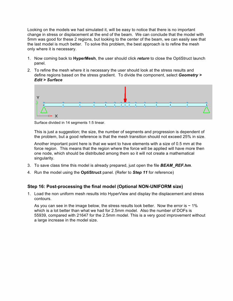
2. To refine the mesh where it is necessary the user should look at the stress results and define regions based on the stress gradient. To divide the component, select Geometry > Edit > Surface

Surface divided in 14 segments 1:5 linear.

This is just a suggestion; the size, the number of segments and progression is dependent of the problem, but a good reference is that the mesh transition should not exceed 25% in size.

Another important point here is that we want to have elements with a size of 0.5 mm at the force region. This means that the region where the force will be applied will have more then one node, which should be distributed among them so it will not create a mathematical singularity.

3. To save class time this model is already prepared, just open the file BEAM_REF.hm.

4. Run the model using the OptiStruct panel. (Refer to Step 11 for reference)

Step 16: Post-processing the final model (Optional NON-UNIFORM size) 1. Load the non uniform mesh results into HyperView and display the displacement and stress

contours.

As you can see in the image below, the stress results look better. Now the error is ~ 1% which is a lot better than what we had for 2.5mm model. Also the number of DOFs is 55939, compared with 21647 for the 2.5mm model. This is a very good improvement without a large increase in the model size.

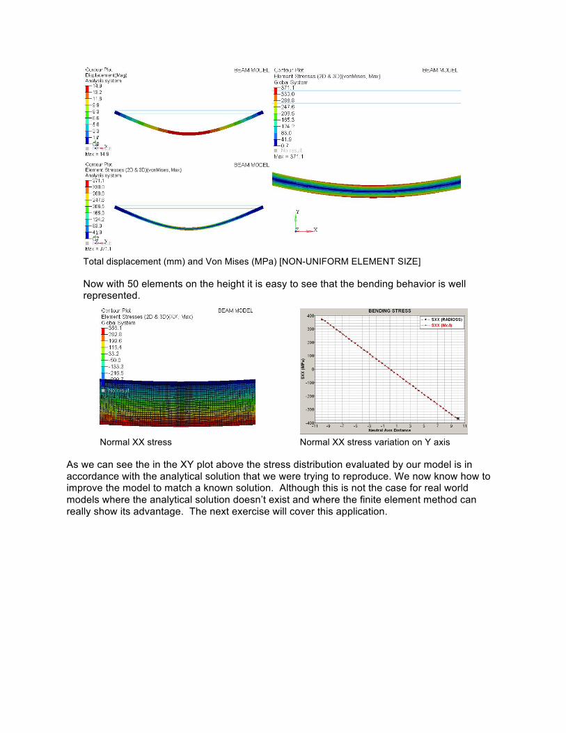
Total displacement (mm) and Von Mises (MPa) [NON-UNIFORM ELEMENT SIZE]

Now with 50 elements on the height it is easy to see that the bending behavior is well represented.

Normal XX stress Normal XX stress variation on Y axis

As we can see the in the XY plot above the stress distribution evaluated by our model is in accordance with the analytical solution that we were trying to reproduce. We now know how to improve the model to match a known solution. Although this is not the case for real world models where the analytical solution doesn’t exist and where the finite element method can really show its advantage. The next exercise will cover this application.