Embed Size (px)
Citation preview

Exercise 17-1 (15 minutes)
1.
2002
2001Sales.............................................................. 100.0% 100.0 %
Less cost of goods sold.................................... 63.2 60.0 Gross margin .................................................. 36.8 40.0
Selling expenses ............................................. 18.0 17.5Administrative expenses .................................. 13.6 14.6
Total expenses................................................ 31.6 32.1 Net operating income ...................................... 5.2 7.9 Interest expense............................................. 1.4 1.0 Net income before taxes.................................. 3.8% 6.9%
Exercise 17-3 (20 minutes)
1. Return on total assets:
( )
( )( )
Net income+ Interest expense× 1-Tax rateReturn on =total assets Average total assets
$470,000+ $90,000× 1 - 0.30=
1/2 $5,000,000 + $4,800,000
$533,000= =10.9% (rounded)
$4,900,000
é ùë û
é ùë û
2. Return on common stockholders’ equity:
Net income as reported ........................................ $ 470,000 Less preferred dividends: 7% × $800,000.............. 56,000 Net income remaining for common (a)................... $ 414,000
Average stockholders’ equity: 1/2 ($3,100,000 + $2,900,000) .......................... $3,000,000
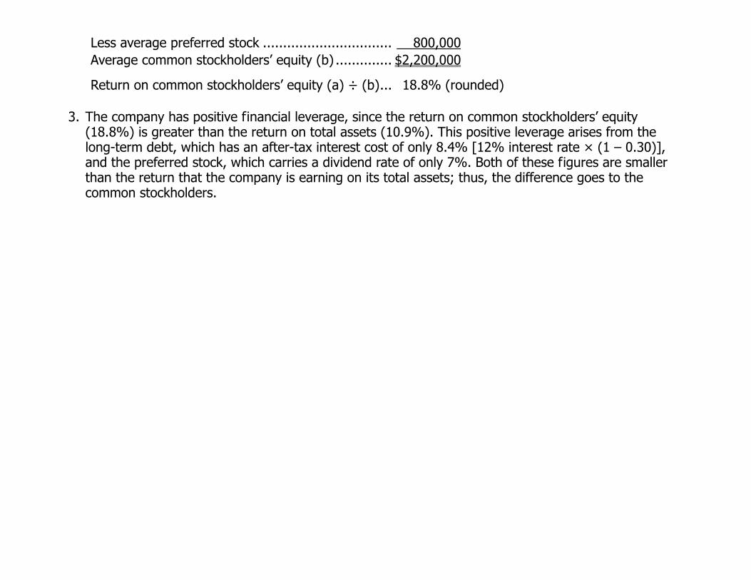
Less average preferred stock ................................ 800,000 Average common stockholders’ equity (b) .............. $2,200,000
Return on common stockholders’ equity (a) ÷ (b)... 18.8% (rounded) 3. The company has positive financial leverage, since the return on common stockholders’ equity
(18.8%) is greater than the return on total assets (10.9%). This positive leverage arises from the long-term debt, which has an after-tax interest cost of only 8.4% [12% interest rate × (1 – 0.30)], and the preferred stock, which carries a dividend rate of only 7%. Both of these figures are smaller than the return that the company is earning on its total assets; thus, the difference goes to the common stockholders.
Problem 17-9 (30 minutes)
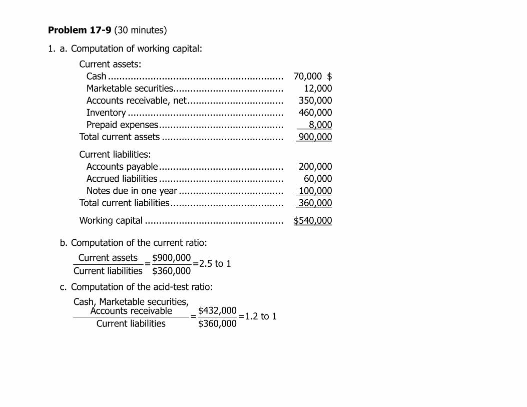
1. a. Computation of working capital:
Current assets: Cash ............................................................... 70,000 $Marketable securities........................................ 12,000Accounts receivable, net................................... 350,000Inventory ........................................................ 460,000Prepaid expenses............................................. 8,000
Total current assets ............................................ 900,000
Current liabilities: Accounts payable............................................. 200,000Accrued liabilities ............................................. 60,000Notes due in one year ...................................... 100,000
Total current liabilities......................................... 360,000
Working capital .................................................. $540,000 b. Computation of the current ratio:
Current assets $900,000
= =2.5 to 1Current liabilities $360,000
c. Computation of the acid-test ratio:
Cash, Marketable securities,$432,000Accounts receivable = =1.2 to 1
Current liabilities $360,000

Problem 17-9 (continued)
2. The Effect on Working Current Acid-Test
Transaction Capital Ratio Ratio (a) Declared a cash dividend......... Decrease Decrease Decrease (b) Paid accounts payable ............. None Increase Increase
(c) Collected cash on accounts
receivable............................ None None None
(d) Purchased equipment for
cash.................................... Decrease Decrease Decrease
(e) Paid a cash dividend
previously declared .............. None Increase Increase
(f) Borrowed cash on a short-
term note ............................ None Decrease Decrease (g) Sold inventory at a profit......... Increase Increase Increase
(h) Wrote off uncollectible
accounts.............................. None None None
(i) Sold marketable securities at
a loss .................................. Decrease Decrease Decrease (j) Issued capital stock for cash Increase Increase Increase (k) Paid off short-term notes......... None Increase Increase

Problem 17-12 (90 minutes)
1.
a.
This Year Last YearNet income............................................. $ 280,000 $ 168,000
Add after-tax cost of interest: $120,000 × (1 – 0.30) .......................... 84,000 $100,000 × (1 – 0.30) .......................... 70,000 Total (a)................................................. $ 364,000 $ 238,000
Average total assets (b)........................... $5,330,000 $4,640,000 Return on total assets (a) ÷ (b) ............... 6.8% 5.1%
b. Net income............................................. $ 280,000 $ 168,000
Less preferred dividends.......................... 48,000 48,000 Net income remaining for common (a) ..... $ 232,000 $ 120,000
Average total stockholders’ equity ............ $3,120,000 $3,028,000 Less average preferred stock ................... 600,000 600,000 Average common equity (b)..................... $2,520,000 $2,428,000
Return on common equity (a) ÷ (b) ......... 9.2% 4.9%
c. Leverage is positive for this year, since the return on common equity (9.2%) is greater than the return on total assets (6.8%). For last year, leverage is negative since the return on the common equity (4.9%) is less than the return on total assets (5.1%).
2. a. Net income remaining for common (a) ..... $ 232,000 $ 120,000 Average number of common shares (b) .... 50,000 50,000 Earnings per share (a) ÷ (b).................... $4.64 $2.40 b. Common dividend per share (a) ............... $1.44 $0.72

Market price per share (b) ....................... $36.00 $20.00 Dividend yield ratio (a) ÷ (b) ................... 4.0% 3.6%
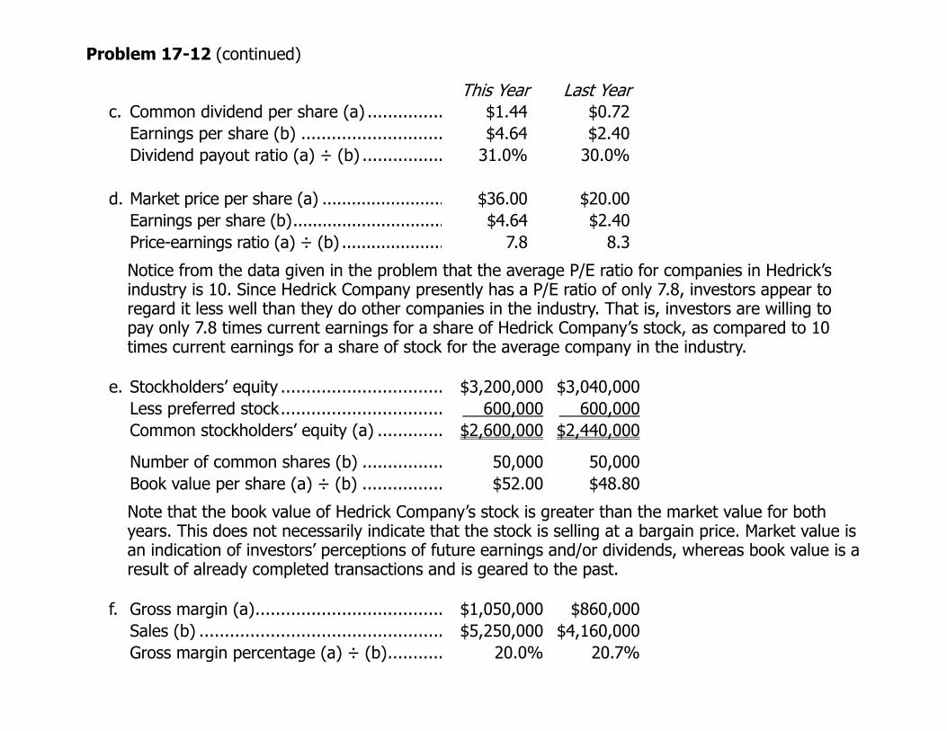
Problem 17-12 (continued)
This Year Last Year c. Common dividend per share (a) ............... $1.44
$0.72 Earnings per share (b) ............................ $4.64 $2.40
Dividend payout ratio (a) ÷ (b) ................ 31.0%
30.0%
d. Market price per share (a) ......................... $36.00 $20.00 Earnings per share (b)............................... $4.64 $2.40 Price-earnings ratio (a) ÷ (b) ..................... 7.8
8.3
Notice from the data given in the problem that the average P/E ratio for companies in Hedrick’s industry is 10. Since Hedrick Company presently has a P/E ratio of only 7.8, investors appear to regard it less well than they do other companies in the industry. That is, investors are willing to pay only 7.8 times current earnings for a share of Hedrick Company’s stock, as compared to 10 times current earnings for a share of stock for the average company in the industry.
e. Stockholders’ equity ................................ $3,200,000 $3,040,000
Less preferred stock................................ 600,000 600,000 Common stockholders’ equity (a) ............. $2,600,000 $2,440,000
Number of common shares (b) ................ 50,000 50,000 Book value per share (a) ÷ (b) ................ $52.00 $48.80
Note that the book value of Hedrick Company’s stock is greater than the market value for both years. This does not necessarily indicate that the stock is selling at a bargain price. Market value is an indication of investors’ perceptions of future earnings and/or dividends, whereas book value is a result of already completed transactions and is geared to the past.
f. Gross margin (a)..................................... $1,050,000 $860,000 Sales (b) ................................................ $5,250,000 $4,160,000 Gross margin percentage (a) ÷ (b)........... 20.0% 20.7%

Problem 17-12 (continued)
3.
a.
This Year Last YearCurrent assets ......................................... $2,600,000 $1,980,000
Current liabilities...................................... 1,300,000 920,000 Working capital........................................ $1,300,000 $1,060,000
b. Current assets (a) .................................... $2,600,000 $1,980,000
Current liabilities (b) ................................ $1,300,000 $920,000 Current ratio (a) ÷ (b).............................. 2.0 to 1 2.15 to 1 c. Quick assets (a)....................................... $1,220,000 $1,120,000 Current liabilities (b) ................................ $1,300,000 $920,000 Acid-test ratio (a) ÷ (b)............................ 0.94 to 1 1.22 to 1
d. Sales on account (a) ................................ $5,250,000 $4,160,000
Average receivables (b) ............................ $750,000 $560,000 Accounts receivable turnover (a) ÷ (b) ...... 7.0 times 7.4 times
Average age of receivables,
365 ÷ turnover ..................................... 52 days 49 days e. Cost of goods sold (a) .............................. $4,200,000 $3,300,000 Average inventory (b)............................... $1,050,000 $720,000 Inventory turnover (a) ÷ (b)..................... 4.0 times 4.6 times
Number of days to turn inventory, 365
days ÷ turnover (rounded)..................... 91 days 79 days f. Total liabilities (a) .................................... $2,500,000 $1,920,000 Stockholders’ equity (b)............................ $3,200,000 $3,040,000 Debt-to-equity ratio (a) ÷ (b).................... 0.78 to 1 0.63 to 1
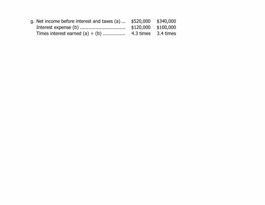
g. Net income before interest and taxes (a) ... $520,000 $340,000 Interest expense (b) ................................ $120,000 $100,000 Times interest earned (a) ÷ (b) ................ 4.3 times 3.4 times
Problem 17-12 (continued)
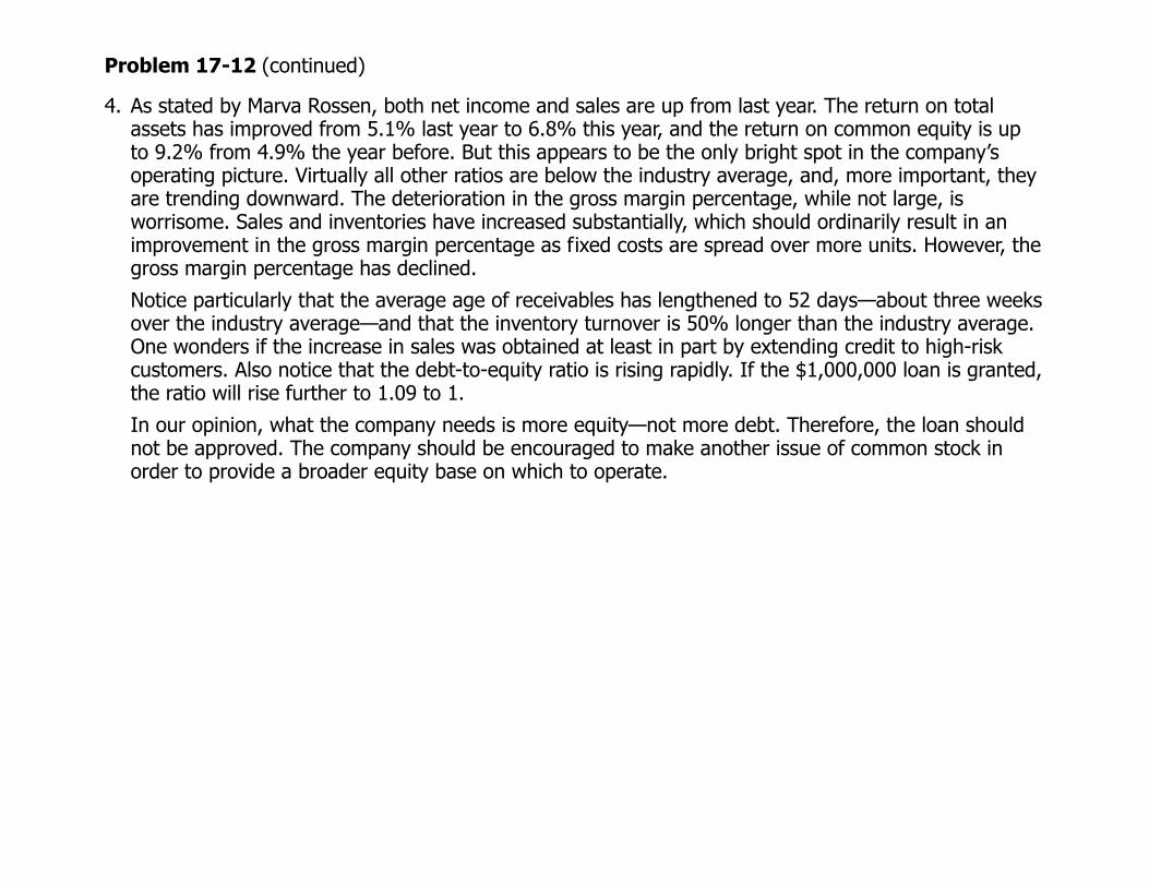
4. As stated by Marva Rossen, both net income and sales are up from last year. The return on total assets has improved from 5.1% last year to 6.8% this year, and the return on common equity is up to 9.2% from 4.9% the year before. But this appears to be the only bright spot in the company’s operating picture. Virtually all other ratios are below the industry average, and, more important, they are trending downward. The deterioration in the gross margin percentage, while not large, is worrisome. Sales and inventories have increased substantially, which should ordinarily result in an improvement in the gross margin percentage as fixed costs are spread over more units. However, the gross margin percentage has declined.
Notice particularly that the average age of receivables has lengthened to 52 days—about three weeks over the industry average—and that the inventory turnover is 50% longer than the industry average. One wonders if the increase in sales was obtained at least in part by extending credit to high-risk customers. Also notice that the debt-to-equity ratio is rising rapidly. If the $1,000,000 loan is granted, the ratio will rise further to 1.09 to 1.
In our opinion, what the company needs is more equity—not more debt. Therefore, the loan should not be approved. The company should be encouraged to make another issue of common stock in order to provide a broader equity base on which to operate.
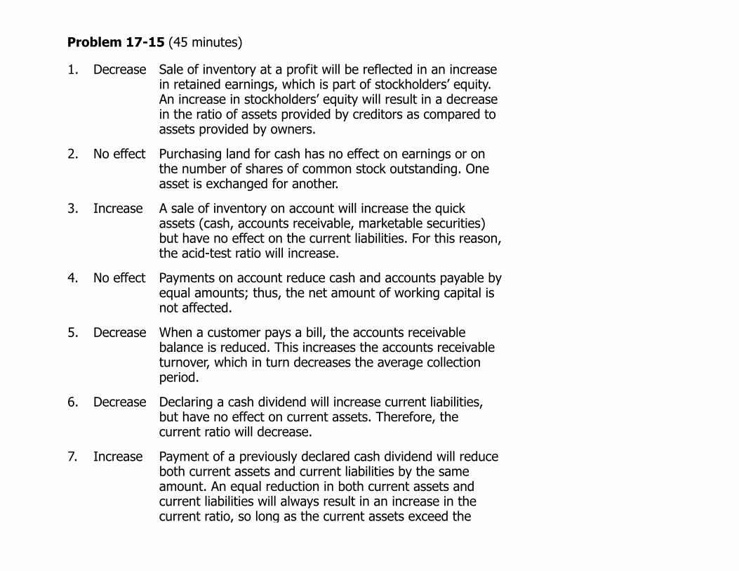
Problem 17-15 (45 minutes)
1. Decrease Sale of inventory at a profit will be reflected in an increase in retained earnings, which is part of stockholders’ equity. An increase in stockholders’ equity will result in a decrease in the ratio of assets provided by creditors as compared to assets provided by owners.
2. No effect Purchasing land for cash has no effect on earnings or on the number of shares of common stock outstanding. One asset is exchanged for another.
3. Increase A sale of inventory on account will increase the quick assets (cash, accounts receivable, marketable securities) but have no effect on the current liabilities. For this reason, the acid-test ratio will increase.
4. No effect Payments on account reduce cash and accounts payable by equal amounts; thus, the net amount of working capital is not affected.
5. Decrease When a customer pays a bill, the accounts receivable balance is reduced. This increases the accounts receivable turnover, which in turn decreases the average collection period.
6. Decrease Declaring a cash dividend will increase current liabilities, but have no effect on current assets. Therefore, the current ratio will decrease.
7. Increase Payment of a previously declared cash dividend will reduce both current assets and current liabilities by the same amount. An equal reduction in both current assets and current liabilities will always result in an increase in the current ratio, so long as the current assets exceed the

current liabilities.
8. No effect Book value per share is not affected by the current market price of the company’s stock.

Problem 17-15 (continued)
9. Decrease The dividend yield ratio is obtained by dividing the dividend per share by the market price per share. If the dividend per share remains unchanged and the market price goes up, then the yield will decrease.
10. Increase Selling property for a profit would increase net income and therefore the return on total assets would increase.
11. Increase A write-off of inventory will reduce the inventory balance, thereby increasing the turnover in relation to a given level of cost of goods sold.
12. Increase Since the company’s assets earn at a rate that is higher than the rate paid on the bonds, leverage is positive, increasing the return to the common stockholders.
13. No effect Changes in the market price of a stock have no direct effect on the dividends paid or on the earnings per share and therefore have no effect on this ratio.
14. Decrease A decrease in net income would mean less income available to cover interest payments. Therefore, the times-interest-earned ratio would decrease.
15. No effect Write-off of an uncollectible account against the Allowance for Bad Debts will have no effect on total current assets. For this reason, the current ratio will remain unchanged.
16. Decrease A purchase of inventory on account will increase current liabilities, but will not increase the quick assets (cash, accounts receivable, marketable securities). Therefore, the ratio of quick assets to current liabilities will decrease.
17. Increase The price-earnings ratio is obtained by dividing the market

price per share by the earnings per share. If the earnings per share remains unchanged, and the market price goes up, then the price-earnings ratio will increase.
18. Decrease Payments to creditors will reduce the total liabilities of a company, thereby decreasing the ratio of total debt to total equity.
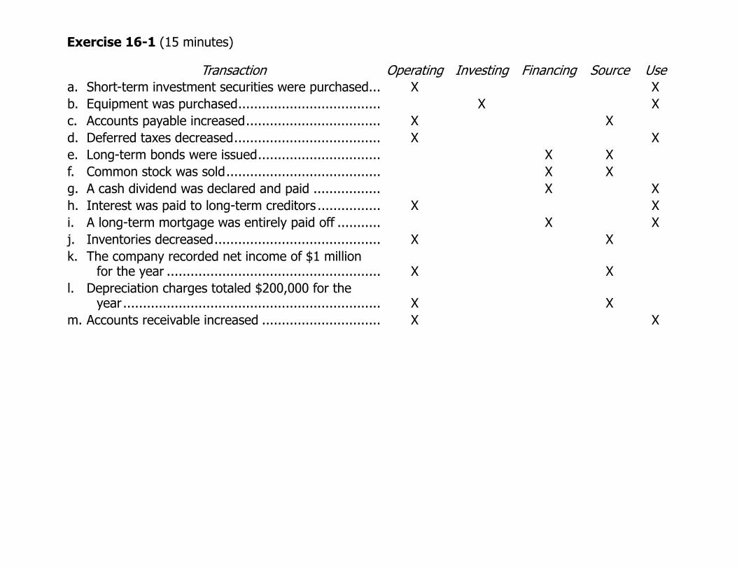
Exercise 16-1 (15 minutes)
T ans ti nr ac o
Operating Investing Financing Source Usea. Short-term investment securities were purchased... X X b. Equipment was purchased.................................... X Xc. Accounts payable increased.................................. X Xd. Deferred taxes decreased..................................... X Xe.
Long-term bonds were issued............................... X X f. Common stock was sold....................................... X Xg. A cash dividend was declared and paid ................. X Xh. Interest was paid to long-term creditors ................ X X i. A long-term mortgage was entirely paid off ........... X X j. Inventories decreased.......................................... X Xk. The company recorded net income of $1 million
for the year ...................................................... X Xl. Depreciation charges totaled $200,000 for the
year ................................................................. X Xm. Accounts receivable increased .............................. X X

Exercise 16-2 (10 minutes)
Item Amount Add DeductAccounts Receivable ..................... 70,000 $ decrease X Accrued Interest Receivable .......... 6,000 increase X Inventory..................................... 110,000 increase X Prepaid Expenses ......................... 3,000 decrease X Accounts Payable ......................... 40,000 decrease X Accrued Liabilities......................... 9,000 increase X Deferred Income Taxes ................. 15,000 increase X Sale of equipment ........................ 8,000 gain X Sale of long-term investments ....... 12,000 loss X Exercise 16-4 (15 minutes)
Sales ............................................................... $1,000,000 Adjustments to a cash basis:
Less increase in accounts receivable ............. 60,000 – $940,000
Cost of goods sold............................................ 580,000 Adjustments to a cash basis:
Plus increase in inventory............................. 77,000 + Less increase in accounts payable................. 30,000 – 627,000
Operating expenses.......................................... 300,000 Adjustments to a cash basis:
Less decrease in prepaid expenses ............... 2,000 – Plus decrease in accrued liabilities ................ 4,000 + Less depreciation charges ............................ 50,000 – 252,000
Income taxes ................................................... 36,000 Adjustments to a cash basis:
Less increase in deferred income taxes ......... 6,000 – 30,000
Net cash provided by operating activities............ 31,000 $
Note that the $31,000 agrees with the cash provided by operating activities figure under the indirect method in the previous exercise.

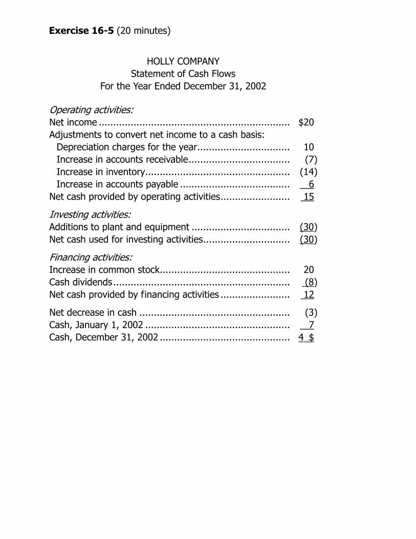
Exercise 16-5 (20 minutes)
HOLLY COMPANY
Statement of Cash Flows For the Year Ended December 31, 2002
Operating activities: Net income ................................................................... $20 Adjustments to convert net income to a cash basis:
Depreciation charges for the year................................. 10 Increase in accounts receivable.................................... (7) Increase in inventory................................................... (14) Increase in accounts payable ....................................... 6
Net cash provided by operating activities......................... 15
Investing activities: Additions to plant and equipment ................................... (30) Net cash used for investing activities............................... (30)
Financing activities: Increase in common stock.............................................. 20 Cash dividends.............................................................. (8) Net cash provided by financing activities ......................... 12
Net decrease in cash ..................................................... (3) Cash, January 1, 2002 ................................................... 7 Cash, December 31, 2002 .............................................. 4 $
Exercise 16-5 (continued)
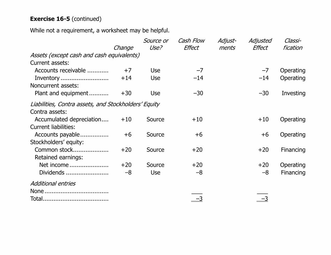
While not a requirement, a worksheet may be helpful.
Change Source or
Use? Cash Flow
Effect Adjust-ments
Adjusted Effect
Classi-fication
Assets (except cash and cash equivalents) Current assets:
Accounts receivable ............ +7 Use –7 –7 OperatingInventory ........................... +14
Use –14 –14 OperatingNoncurrent assets:
Plant and equipment ........... +30 Use –30 –30 Investing
Liabilities, Contra assets, and Stockholders’ Equity Contra assets:
Accumulated depreciation.... +10 Source +10 +10 OperatingCurrent liabilities:
Accounts payable................ +6 Source +6 +6 OperatingStockholders’ equity:
Common stock.................... +20 Source +20 +20 FinancingRetained earnings:
Net income ...................... +20 Source +20 +20 OperatingDividends ........................ –8 Use –8 –8 Financing
Additional entries None .................................... Total..................................... –3 –3
Exercise 16-5 (20 minutes)
HOLLY COMPANY
Statement of Cash Flows For the Year Ended December 31, 2002
Operating activities: Net income ................................................................... $20 Adjustments to convert net income to a cash basis:
Depreciation charges for the year................................. 10 Increase in accounts receivable.................................... (7) Increase in inventory................................................... (14) Increase in accounts payable ....................................... 6
Net cash provided by operating activities......................... 15
Investing activities: Additions to plant and equipment ................................... (30) Net cash used for investing activities............................... (30)
Financing activities: Increase in common stock.............................................. 20 Cash dividends.............................................................. (8) Net cash provided by financing activities ......................... 12
Net decrease in cash ..................................................... (3) Cash, January 1, 2002 ................................................... 7 Cash, December 31, 2002 .............................................. 4 $

Problem 16-10 (30 minutes)
1. and 2. EATON COMPANY Statement of Cash Flows For the Year Ended December 31, 2002
Operating activities: Net income.......................................................... 56 $ Adjustments to convert net income to cash basis:
Depreciation charges....................................... 25 Increase in accounts receivable ........................ (80) Decrease in inventory...................................... 35 Increase in prepaid expenses ........................... (2) Increase in accounts payable ........................... 75 Decrease in accrued liabilities........................... (10) Gain on sale of investments ............................. (5) Loss on sale of equipment ............................... 2 Increase in deferred income taxes .................... 8
Net cash provided by operating activities ............... 104
Investing activities: Proceeds from sale of long-term investments ......... 12 Proceeds from sale of equipment........................... 18 Additions to plant and equipment .......................... (110) Net cash used for investing activities ..................... (80)
Financing activities: Increase in bonds payable .................................... 25 Decrease in common stock ................................... (40) Cash dividends..................................................... (16) Net cash used for financing activities ..................... (31)
Net decrease in cash ............................................ (7) Cash balance, January 1, 2002.............................. 11 Cash balance, December 31, 2002......................... 4 $
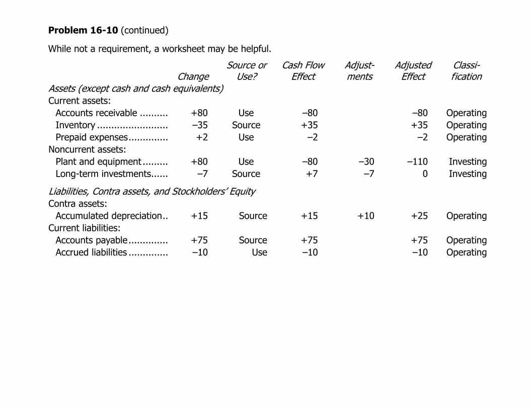
Problem 16-10 (continued)
While not a requirement, a worksheet may be helpful.
Change Source or
Use? Cash Flow
Effect Adjust-ments
Adjusted Effect
Classi-fication
Assets (except cash and cash equivalents) Current assets:
Accounts receivable .......... +80 Use –80 –80 OperatingInventory ......................... –35
Source +35 +35 OperatingPrepaid expenses.............. +2 Use –2 –2 Operating
Noncurrent assets: Plant and equipment ......... +80 Use –80 –30 –110 InvestingLong-term investments......
–7 Source +7 –7 0 Investing
Liabilities, Contra assets, and Stockholders’ Equity Contra assets:
Accumulated depreciation.. +15 Source +15 +10 +25 OperatingCurrent liabilities:
Accounts payable.............. +75 Source +75 +75 OperatingAccrued liabilities .............. –10 Use –10 –10 Operating

Problem 16-10 (continued)
Change Source or
Use? Cash Flow
Effect Adjust-ments
Adjusted Effect
Classi-fication
Noncurrent liabilities: Bonds payable .................. +25 Source
+25 +25 FinancingDeferred income taxes ...... +8 Source +8 +8 Operating
Stockholders’ equity: Common stock.................. –40 Use –40 –40 FinancingRetained earnings:
Net income .................... +56 Source +56 +56 OperatingDividends ......................
–16 Use –16 –16
Financing
Additional entries Proceeds from sale of
equipment........................ +18 +18 InvestingLoss on sale of equipment.... +2 +2 OperatingProceeds from sale of long-
term investments.............. +12 +12 InvestingGain on sale of long-term
investments...................... –5 –5
Operating
Total................................... –7 0 –7
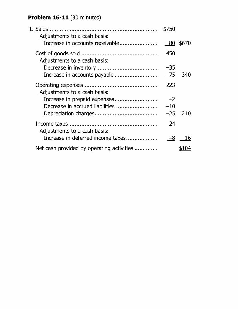
Problem 16-11 (30 minutes)
1. Sales.................................................................. $750 Adjustments to a cash basis: Increase in accounts receivable....................... –80 $670
Cost of goods sold .............................................. 450 Adjustments to a cash basis: Decrease in inventory..................................... –35 Increase in accounts payable .......................... –75 340
Operating expenses ............................................ 223 Adjustments to a cash basis: Increase in prepaid expenses.......................... +2 Decrease in accrued liabilities ......................... +10 Depreciation charges...................................... –25 210
Income taxes...................................................... 24 Adjustments to a cash basis: Increase in deferred income taxes................... –8 16
Net cash provided by operating activities .............. $104

Problem 16-11 (continued)
2. EATON COMPANY Statement of Cash Flows For the Year ended December 31, 2002
Operating activities: Cash received from customers.............................. $670 Less cash disbursements for:
Cost of merchandise sold .................................. $340 Operating expenses .......................................... 210 Income taxes ................................................... 16
Total cash disbursements..................................... 566 Net cash provided by operating activities .............. 104
Investing activities: Proceeds from sale of long-term investments ........ 12 Proceeds from sale of equipment.......................... 18 Additions to plant and equipment ......................... (110) Net cash used for investing activities .................... (80)
Financing activities: Increase in bonds payable ................................... 25 Decrease in common stock .................................. (40) Cash dividends.................................................... (16) Net cash used for financing activities .................... (31)
Net decrease in cash ........................................... (7)Cash balance, January 1, 2002............................. 11 Cash balance, December 31, 2002........................ 4 $

Problem 16-12 (45 minutes)
1. and 2. FOXBORO COMPANY Statement of Cash Flows For Year 2
Operating activities: Net income........................................................ 63,000 $ Adjustments to convert net income to cash basis:
Depreciation charges ....................................... $ 45,000 Increase in accounts receivable ........................ (70,000) Increase in inventory ....................................... (48,000) Decrease in prepaid expenses .......................... 9,000 Increase in accounts payable............................ 50,000 Decrease in accrued liabilities........................... (8,000) Gain on sale of equipment ............................... (6,000) Increase in deferred income taxes .................... 4,000 (24,000)
Net cash provided by operating activities ............. 39,000
Investing activities: Proceeds from sale of equipment ........................ 26,000 Loan to Harker Company .................................... (40,000) Additions to plant and equipment........................ (150,000) Net cash used for investing activities ................... (164,000)
Financing activities: Increase in bonds payable .................................. 90,000 Increase in common stock .................................. 60,000 Cash dividends .................................................. (33,000) Net cash provided by financing activities.............. 117,000
Net decrease in cash.......................................... (8,000) Cash balance, beginning of year.......................... 19,000 Cash balance, end of year .................................. 11,000 $

Problem 16-12 (continued)
3. The relatively small amount of cash provided by operating activities during the year was largely the result of a large increase in accounts receivable. (The large increase in inventory was offset by a large increase in accounts payable.) Most of the cash that was provided by operating activities was paid out in dividends. The small amount that remained, combined with the cash provided by the issue of bonds and the issue of common stock, was insufficient to purchase a large amount of equipment and make a loan to another company. As a result, the cash on hand declined sharply during the year.

Problem 16-12 (continued)
While not a requirement, a worksheet may be helpful.
Change Source or
Use? Cash Flow
Effect Adjust-ments
Adjusted Effect
Classi-fication
Assets (except cash and cash equivalents) Current assets:
Accounts receivable ............ +70
Use –70 –70 OperatingInventory ........................... +48 Use –48 –48 OperatingPrepaid expenses................ –9 Source +9 +9 Operating
Noncurrent assets: Loan to Harker Company..... +40 Use –40 –40 InvestingPlant and equipment ........... +120 Use –120 –30 –150 Investing
Liabilities, Contra assets, and Stockholders’ Equity Contra assets:
Accumulated depreciation.... +35 Source +35 +10 +45 OperatingCurrent liabilities:
Accounts payable................ +50 Source +50 +50 OperatingAccrued liabilities ................ –8 Use –8 –8 Operating
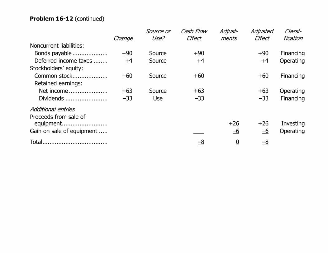
Problem 16-12 (continued)
Change Source or
Use? Cash Flow
Effect Adjust-ments
Adjusted Effect
Classi-fication
Noncurrent liabilities: Bonds payable .................... +90 Source
+90 +90 FinancingDeferred income taxes ........ +4 Source +4 +4 Operating
Stockholders’ equity: Common stock.................... +60 Source +60 +60 FinancingRetained earnings:
Net income ...................... +63 Source +63 +63 OperatingDividends ........................ –33 Use –33 –33 Financing
Additional entries Proceeds from sale of
equipment.......................... +26 +26 InvestingGain on sale of equipment ..... –6 –6 Operating
Total..................................... –8 0 –8
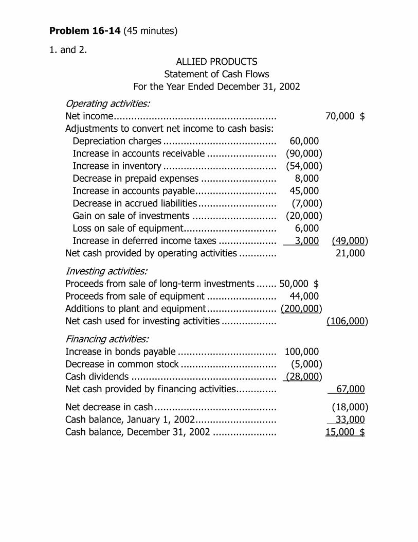
Problem 16-14 (45 minutes)
1. and 2. ALLIED PRODUCTS Statement of Cash Flows For the Year Ended December 31, 2002
Operating activities: Net income........................................................ 70,000 $ Adjustments to convert net income to cash basis:
Depreciation charges ....................................... 60,000 Increase in accounts receivable ........................ (90,000) Increase in inventory ....................................... (54,000) Decrease in prepaid expenses .......................... 8,000 Increase in accounts payable............................ 45,000 Decrease in accrued liabilities ........................... (7,000) Gain on sale of investments ............................. (20,000) Loss on sale of equipment................................ 6,000 Increase in deferred income taxes .................... 3,000 (49,000)
Net cash provided by operating activities ............. 21,000
Investing activities: Proceeds from sale of long-term investments ....... 50,000 $ Proceeds from sale of equipment ........................ 44,000 Additions to plant and equipment........................ (200,000) Net cash used for investing activities ................... (106,000)
Financing activities: Increase in bonds payable .................................. 100,000
Decrease in common stock ................................. (5,000) Cash dividends .................................................. (28,000) Net cash provided by financing activities.............. 67,000
Net decrease in cash .......................................... (18,000) Cash balance, January 1, 2002............................ 33,000 Cash balance, December 31, 2002 ...................... 15,000 $

Problem 16-14 (continued)
3. Although the company reported a large net income for the year, a relatively small amount of cash was provided by operating activities due to increases in both accounts receivable and inventory. Note particularly that operations didn’t generate enough cash to even pay the cash dividends for the year. Although the company obtained cash from sales of assets and an issue of bonds, this was not sufficient to cover the cost of a $200,000 increase in plant and equipment for the year. More care should have been taken in planning this major investment in plant assets. Also, the company should probably get better control over its accounts receivable. (Although inventory also increased during the year, this increase was largely offset by the increase in accounts payable.)

Problem 16-14 (continued)
While not a requirement, a worksheet may be helpful.
Change Source or
Use?
Cash Flow Effect
Adjust-ments
Adjusted Effect
Classi-fication
Assets (except cash and cash equivalents) Current assets:
Accounts receivable ............ +90
Use –90 –90 OperatingInventory ........................... +54 Use –54 –54 OperatingPrepaid expenses................ –8 Source +8 +8 Operating
Noncurrent assets: Long-term investments........ –30 Source +30 –30 0 InvestingPlant and equipment ........... +110 Use –110 –90 –200 Investing
Liabilities, Contra assets, and Stockholders’ Equity Contra assets:
Accumulated depreciation.... +20 Source +20 +40 +60 OperatingCurrent liabilities:
Accounts payable................ +45 Source +45 +45 OperatingAccrued liabilities ................ –7 Use –7 –7 Operating

Problem 16-14 (continued)
Change Source or
Use?
Cash Flow Effect
Adjust-ments
Adjusted Effect
Classi-fication
Noncurrent liabilities: Bonds payable .................... +100 Source
+100 +100 FinancingDeferred income taxes ........ +3 Source +3 +3 Operating
Stockholders’ equity: Common stock.................... –5 Use –5 –5 FinancingRetained earnings:
Net income ...................... +70 Source +70 +70 OperatingDividends ........................ –28 Use –28 –28 Financing
Additional entries Proceeds from sale of long-
term investments................ +50 +50 InvestingGain from sale of
investments........................ –20 –20 OperatingProceeds from sale of
equipment.......................... +44 +44 InvestingLoss on sale of equipment...... +6 +6
Operating
Total..................................... –18 0 –18
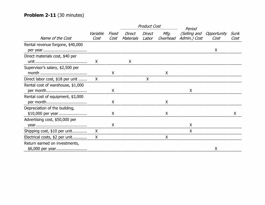
Problem 2-11 (30 minutes)
Product Cost
Name of the Cost Variable
Cost Fixed Cost
Direct Materials
Direct Labor
Mfg. Overhead
Period (Selling and Admin.) Cost
Opportunity Cost
Sunk Cost
Rental revenue forgone, $40,000 per year..................................... X
Direct materials cost, $40 per unit ........................................... X X
Supervisor’s salary, $2,500 per month ....................................... X X
Direct labor cost, $18 per unit ........ X XRental cost of warehouse, $1,000
per month.................................. X XRental cost of equipment, $3,000
per month.................................. X XDepreciation of the building,
$10,000 per year ........................ X X XAdvertising cost, $50,000 per
year........................................... X XShipping cost, $10 per unit............. X XElectrical costs, $2 per unit............. X XReturn earned on investments,
$6,000 per year.......................... X
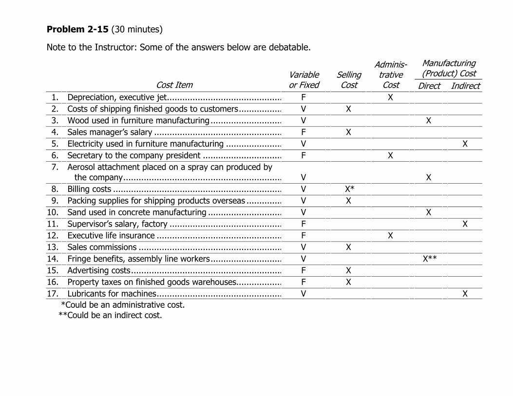
Problem 2-15 (30 minutes)
Note to the Instructor: Some of the answers below are debatable.
Manufacturing (Product) Cost
Cost Item Variable or Fixed
Selling Cost
Adminis-trative Cost Direct Indirect
1. Depreciation, executive jet............................................. F X 2. Costs of shipping finished goods to customers................. V X 3. Wood used in furniture manufacturing............................ V X4. Sales manager’s salary .................................................. F X 5. Electricity used in furniture manufacturing ...................... V X 6. Secretary to the company president ............................... F X 7. Aerosol attachment placed on a spray can produced by
the company.............................................................. V X8. Billing costs .................................................................. V X* 9. Packing supplies for shipping products overseas .............. V X
10. Sand used in concrete manufacturing ............................. V X11. Supervisor’s salary, factory ............................................ F X 12. Executive life insurance ................................................. F X 13. Sales commissions ........................................................ V X 14. Fringe benefits, assembly line workers............................ V X** 15. Advertising costs........................................................... F X 16. Property taxes on finished goods warehouses.................. F X 17. Lubricants for machines................................................. V X
*Could be an administrative cost. **Could be an indirect cost.

Problem 2-19 (60 minutes)
1. MEDCO, INC.
Schedule of Cost of Goods Manufactured
Direct materials: Raw materials inventory, beginning................ $ 10,000Add: Purchases of raw materials .................... 90,000Raw materials available for use...................... 100,000Deduct: Raw materials inventory, ending........ 17,000Raw materials used in production .................. $ 83,000
Direct labor .................................................... 60,000Manufacturing overhead:
Depreciation, factory..................................... 42,000Insurance, factory ........................................ 5,000Maintenance, factory .................................... 30,000Utilities, factory ............................................ 27,000Supplies, factory........................................... 1,000Indirect labor ............................................... 65,000
Total overhead costs ....................................... 170,000Total manufacturing costs................................ 313,000Add: Work in process inventory, beginning........ 7,000 320,000Deduct: Work in process inventory, ending ....... 30,000Cost of goods manufactured ............................ $290,000
Problem 2-19 (continued)
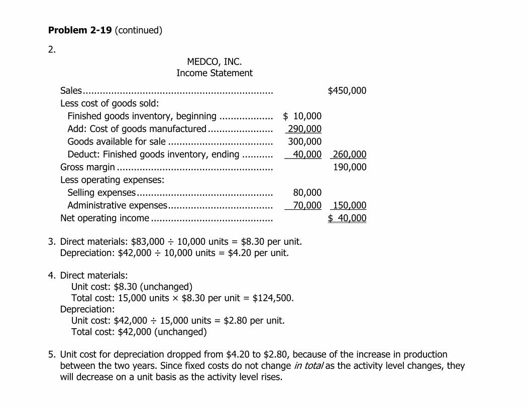
2. MEDCO, INC.
Income Statement
Sales................................................................... $450,000Less cost of goods sold:
Finished goods inventory, beginning ................... $ 10,000 Add: Cost of goods manufactured ....................... 290,000 Goods available for sale ..................................... 300,000 Deduct: Finished goods inventory, ending ........... 40,000 260,000
Gross margin ....................................................... 190,000Less operating expenses:
Selling expenses................................................ 80,000 Administrative expenses..................................... 70,000 150,000
Net operating income ........................................... $ 40,000 3. Direct materials: $83,000 ÷ 10,000 units = $8.30 per unit.
Depreciation: $42,000 ÷ 10,000 units = $4.20 per unit. 4. Direct materials:
Unit cost: $8.30 (unchanged) Total cost: 15,000 units × $8.30 per unit = $124,500.
Depreciation: Unit cost: $42,000 ÷ 15,000 units = $2.80 per unit. Total cost: $42,000 (unchanged)
5. Unit cost for depreciation dropped from $4.20 to $2.80, because of the increase in production
between the two years. Since fixed costs do not change in total as the activity level changes, they will decrease on a unit basis as the activity level rises.

Problem 2-20 (60 minutes) 1.
SKYLER COMPANY Schedule of Cost of Goods Manufactured
For the Month Ended June 30
Direct materials: Raw materials inventory, June 1 .................... $ 17,000Add: Purchases of raw materials .................... 190,000Raw materials available for use...................... 207,000Deduct: Raw materials inventory, June 30 ...... 42,000Raw materials used in production .................. $165,000
Direct labor .................................................... 90,000Manufacturing overhead:
Rent on facilities (80% × $40,000) ............... 32,000Insurance (75% × $8,000) ........................... 6,000Utilities (90% × $50,000) ............................. 45,000Indirect labor ............................................... 108,000Maintenance, factory .................................... 7,000Depreciation, factory equipment .................... 12,000
Total overhead costs ....................................... 210,000Total manufacturing costs................................ 465,000Add: Work in process inventory, June 1 ............ 70,000 535,000Deduct: Work in process inventory, June 30...... 85,000Cost of goods manufactured ............................ $450,000
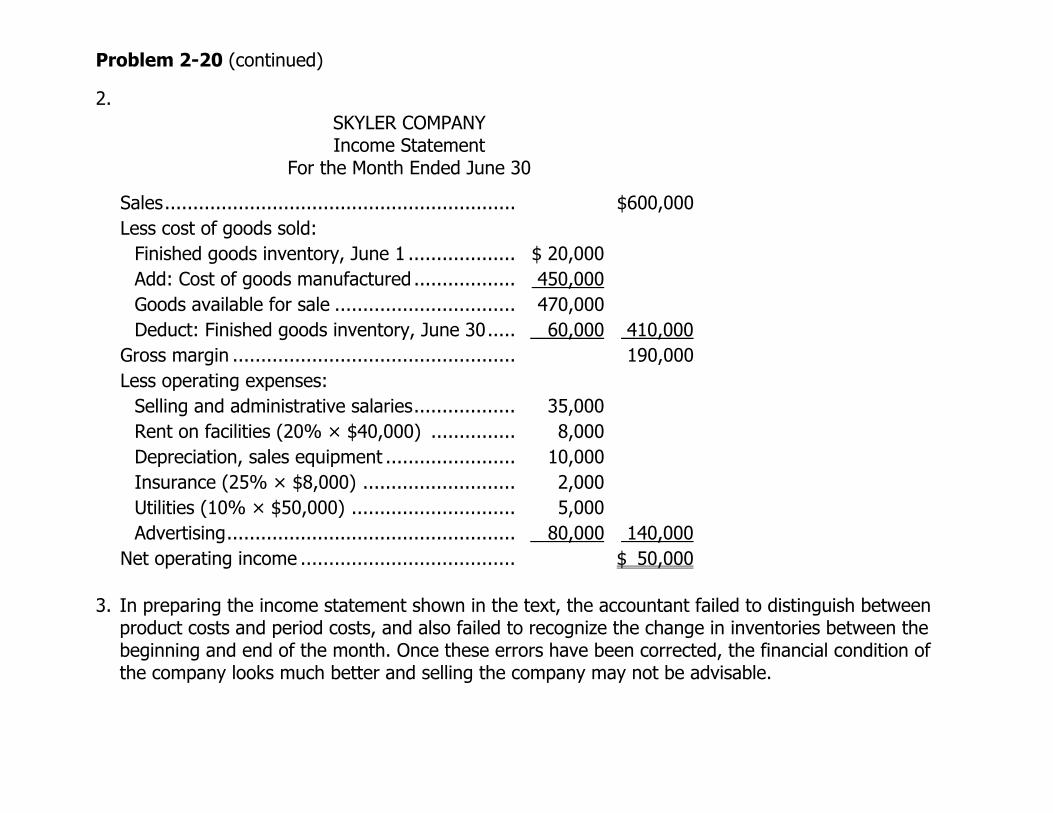
Problem 2-20 (continued)
2. SKYLER COMPANY Income Statement
For the Month Ended June 30
Sales.............................................................. $600,000Less cost of goods sold:
Finished goods inventory, June 1 ................... $ 20,000Add: Cost of goods manufactured .................. 450,000Goods available for sale ................................ 470,000Deduct: Finished goods inventory, June 30..... 60,000 410,000
Gross margin .................................................. 190,000Less operating expenses:
Selling and administrative salaries.................. 35,000Rent on facilities (20% × $40,000) ............... 8,000Depreciation, sales equipment ....................... 10,000Insurance (25% × $8,000) ........................... 2,000Utilities (10% × $50,000) ............................. 5,000Advertising................................................... 80,000 140,000
Net operating income ...................................... $ 50,000 3. In preparing the income statement shown in the text, the accountant failed to distinguish between
product costs and period costs, and also failed to recognize the change in inventories between the beginning and end of the month. Once these errors have been corrected, the financial condition of the company looks much better and selling the company may not be advisable.

Problem 2-21 (60 minutes)
1. VALENKO COMPANY
Schedule of Cost of Goods Manufactured
Direct materials: Raw materials inventory, beginning........... $ 50,000 Add: Purchases of raw materials ............... 260,000 Raw materials available for use................. 310,000 Deduct: Raw materials inventory, ending... 40,000 Raw materials used in production ............. $270,000
Direct labor ............................................... 65,000 * Manufacturing overhead:
Insurance, factory ................................... 8,000 Rent, factory building............................... 90,000 Utilities, factory ....................................... 52,000 Cleaning supplies, factory......................... 6,000 Depreciation, factory equipment ............... 110,000 Maintenance, factory ............................... 74,000
Total overhead costs .................................. 340,000 Total manufacturing costs........................... 675,000 (given)Add: Work in process inventory, beginning... 48,000 * 723,000Deduct: Work in process inventory, ending .. 33,000 Cost of goods manufactured ....................... $690,000

Problem 2-21 (continued)
The cost of goods sold section of the income statement follows:
Finished goods inventory, beginning...................... $ 30,000 Add: Cost of goods manufactured ......................... 690,000
*
Goods available for sale ....................................... 720,000 (given)Deduct: Finished goods inventory, ending.............. 85,000 *Cost of goods sold ............................................... $635,000 (given)
*These items must be computed by working backwards up through the statements. An effective way
of doing this is to place the form and known balances on the chalkboard, and then work toward the unknown figures.
2. Direct materials: $270,000 ÷ 30,000 units = $9.00 per unit.
Rent, factory building: $90,000 ÷ 30,000 units = $3.00 per unit. 3. Direct materials:
Per unit: $9.00 (unchanged) Total: 50,000 units × $9.00 per unit = $450,000.
Rent, factory building: Per unit: $90,000 ÷ 50,000 units = $1.80 per unit. Total: $90,000 (unchanged).
4. The unit cost for rent dropped from $3.00 to $1.80, because of the increase in production between
the two years. Since fixed costs do not change in total as the activity level changes, they will decrease on a unit basis as the activity level rises.
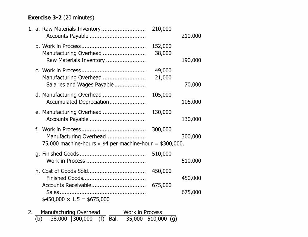
Exercise 3-2 (20 minutes)
1. a. Raw Materials Inventory............................ 210,000 Accounts Payable ................................... 210,000
b. Work in Process........................................ 152,000 Manufacturing Overhead ........................... 38,000 Raw Materials Inventory ......................... 190,000
c. Work in Process........................................ 49,000 Manufacturing Overhead ........................... 21,000 Salaries and Wages Payable .................... 70,000
d. Manufacturing Overhead ........................... 105,000 Accumulated Depreciation....................... 105,000
e. Manufacturing Overhead ........................... 130,000 Accounts Payable ................................... 130,000
f. Work in Process........................................ 300,000 Manufacturing Overhead......................... 300,000
75,000 machine-hours × $4 per machine-hour = $300,000.
g. Finished Goods ......................................... 510,000 Work in Process ..................................... 510,000
h. Cost of Goods Sold.................................... 450,000 Finished Goods....................................... 450,000 Accounts Receivable.................................. 675,000 Sales ..................................................... 675,000 $450,000 × 1.5 = $675,000 2. Manufacturing Overhead
Work in Process
(b) 38,000 300,000 (f) Bal. 35,000 510,000 (g)
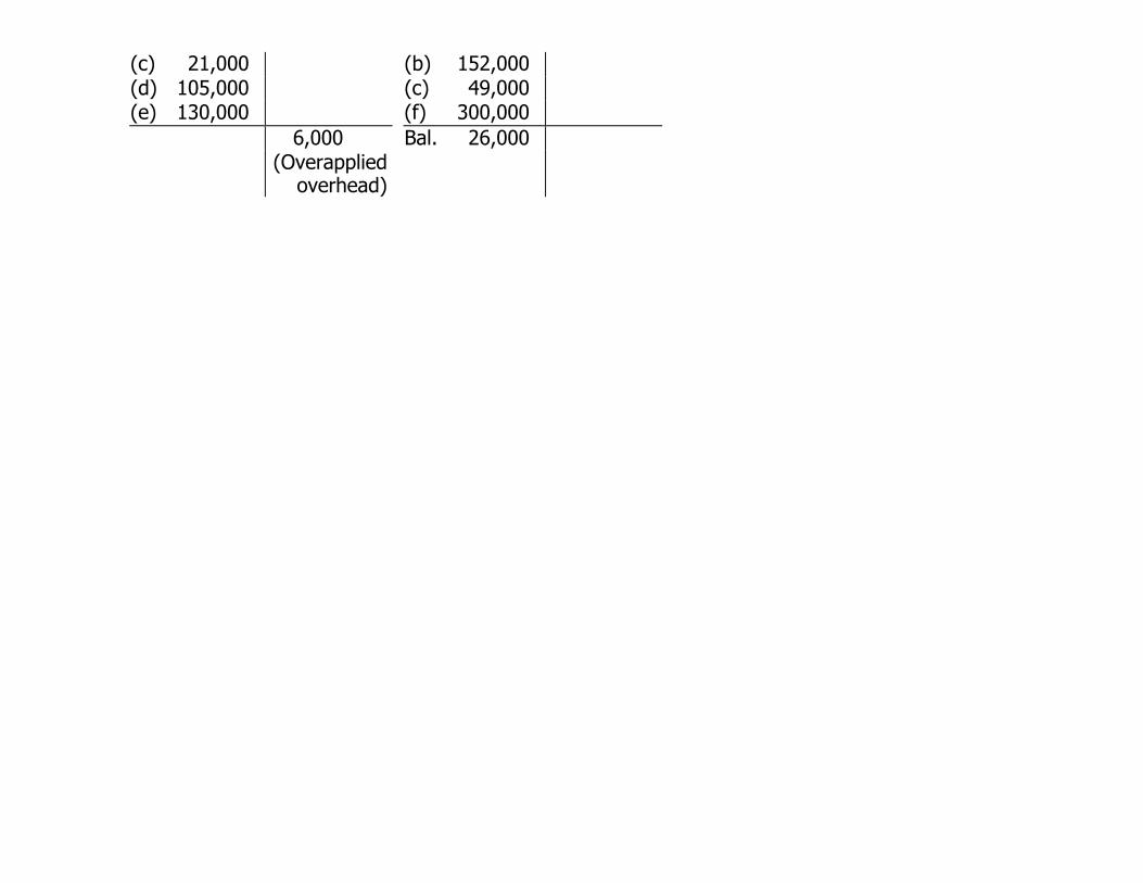
(c) 21,000 (b) 152,000 (d) 105,000 (c) 49,000 (e) 130,000 (f) 300,000 6,000 Bal. 26,000 (Overapplied
overhead)

Exercise 3-3 (15 minutes)
1. Predetermined overhead rates: Company A:
Estimated total manufacturing overhead costPredetermined=overhead rate Estimated total amount of the allocation base
$432,000= =$7.20 per DLH
60,000 DLHs
Company B:
Estimated total manufacturing overhead costPredetermined=overhead rate Estimated total amount of the allocation base
$270,000= =$3.00 per MH
90,000 MHs
Company C:
Estimated total manufacturing overhead costPredetermined=overhead rate Estimated total amount of the allocation base
$384,000= =160% of materials cost
$240,000 materials cost
2. Actual overhead costs incurred........................... $420,000 Overhead cost applied to Work in Process: 58,000* actual hours × $7.20 per hour ............ 417,600 Underapplied overhead cost............................... 2,400 $
*7,000 hours + 30,000 hours + 21,000 hours = 58,000 hours

Exercise 3-5 (15 minutes)
1. Milling Department:
Estimated total manufacturing overhead costPredetermined=overhead rate Estimated total amount of the allocation base
$510,000= =$8.50 per machine-hour
60,000 machine-hours
Assembly Department:
Estimated total manufacturing overhead costPredetermined=overhead rate Estimated total amount of the allocation base
$800,000= =125% of direct labor cost
$640,000 direct labor cost
2. Overhead Applied
Milling Department: 90 MHs × $8.50 per MH ... $765 Assembly Department: $160 × 125%.............. 200 Total overhead cost applied............................ $965 3. Yes; if some jobs required a large amount of machine time and little labor cost, they would be
charged substantially less overhead cost if a plantwide rate based on direct labor cost were being used. It appears, for example, that this would be true of job 407 which required considerable machine time to complete, but required only a small amount of labor cost.

Problem 3-14 (45 minutes)
1. a. Raw Materials ........................................200,000 Accounts Payable.............................. 200,000
b. Work in Process .....................................152,000 Manufacturing Overhead ........................ 38,000 Raw Materials................................... 190,000
c. Work in Process .....................................160,000 Manufacturing Overhead ........................ 27,000 Sales Commissions Expense.................... 36,000 Administrative Salaries Expense .............. 80,000 Salaries and Wages Payable .............. 303,000
d. Manufacturing Overhead ........................ 42,000 Accounts Payable.............................. 42,000
e. Manufacturing Overhead ........................ 9,000 Insurance Expense................................. 1,000 Prepaid Insurance............................. 10,000
f. Advertising Expense ............................... 50,000 Accounts Payable.............................. 50,000
g. Manufacturing Overhead ........................ 51,000 Depreciation Expense............................. 9,000 Accumulated Depreciation ................. 60,000
h. Work in Process .....................................170,000 Manufacturing Overhead ................... 170,000
$153,000=$4.25 per MH; 40,000 MHs×$4.25 per MH=$170,000.
36,000 MHs

Problem 3-14 (continued)
i. Finished Goods ......................................480,000 Work in Process................................ 480,000
j. Accounts Receivable...............................700,000 Sales ............................................... 700,000 Cost of Goods Sold.................................475,000 Finished Goods ................................. 475,000 2. Raw Materials Manufacturing Overhead
Bal. 16,000 190,000 (b) (b) 38,000 170,000 (h) (a) 200,000 (c) 27,000 Bal. 26,000 (d) 42,000 (e) 9,000 (g) 51,000 3,000 Bal.
Work in Process Cost of Goods Sold Bal. 10,000 480,000 (i) (j) 475,000 (b) 152,000 (c) 160,000 (h) 170,000 Bal. 12,000
Finished Goods Bal. 30,000 475,000 (j) (i) 480,000 Bal. 35,000
3. Manufacturing overhead is overapplied by $3,000. The journal entry to close this balance to Cost of
Goods Sold is:

Manufacturing Overhead.............................. 3,000
Cost of Goods Sold ................................. 3,000

Problem 3-14 (continued)
4. RAVSTEN COMPANY Income Statement
For the Year Ended December 31
Sales............................................................ $700,000Less cost of goods sold ($475,000 – $3,000)... 472,000Gross margin ................................................ 228,000Less selling and administrative expenses:
Sales commissions...................................... $36,000Administrative salaries ................................ 80,000Insurance .................................................. 1,000Advertising................................................. 50,000Depreciation............................................... 9,000 176,000
Net operating income .................................... $ 52,000

Problem 3-24 (45 minutes)
1. The cost of raw materials put into production would be:
Raw materials inventory, 1/1 ........................ 30,000 $Debits (purchases of materials) ..................... 420,000Materials available for use............................. 450,000Raw materials inventory, 12/31..................... 60,000Materials requisitioned for production ............ $390,000
2. Of the $390,000 in materials requisitioned for production, $320,000 was debited to Work in Process
as direct materials. Therefore, the difference of $70,000 ($390,000 – $320,000 = $70,000) would have been debited to Manufacturing Overhead as indirect materials.
3. Total factory wages accrued during the year
(credits to the Factory Wages Payable account) .... $175,000 Less direct labor cost (from Work in Process) .......... 110,000 Indirect labor cost................................................. 65,000 $ 4. The cost of goods manufactured for the year would have been $810,000—the credits to Work in
Process. 5. The Cost of Goods Sold for the year would have been:
Finished goods inventory, 1/1 ................................ 40,000 $ Add: Cost of goods manufactured (from Work in
Process)............................................................. 810,000 Goods available for sale......................................... 850,000 Finished goods inventory, 12/31............................. 130,000 Cost of goods sold................................................. $720,000

Problem 3-24 (continued)
6. The predetermined overhead rate would have been:
Manufacturing overhead cost appliedPredetermined=overhead rate Direct materials cost
$400,000= =125% of direct materials cost
$320,000
7. Manufacturing overhead would have been overapplied by $15,000, computed as follows:
Actual manufacturing overhead cost for the year (debits)...................................................................... $385,000
Applied manufacturing overhead cost (from Work in Process—this would be the credits to the Manufacturing Overhead account) ............................... 400,000
Overapplied overhead.................................................... $(15,000) 8. The ending balance in Work in Process is $90,000. Direct labor makes up $18,000 of this balance,
and manufacturing overhead makes up $40,000. The computations are:
Balance, Work in Process, 12/31 ................................. $90,000 Less: Direct materials cost (given) ............................... (32,000)
Manufacturing overhead cost ($32,000 × 125%)............................................................ (40,000)
Direct labor cost (remainder) ...................................... $18,000
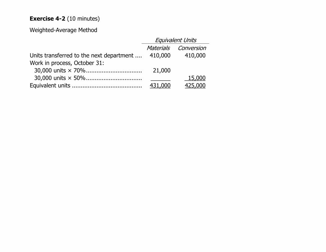
Exercise 4-2 (10 minutes)
Weighted-Average Method
Equivalent Units Materials Conversion
Units transferred to the next department .... 410,000 410,000 Work in process, October 31:
30,000 units × 70%................................ 21,00030,000 units × 50%................................ 15,000
Equivalent units ........................................ 431,000 425,000

Exercise 4-6 (15 minutes)
Weighted-Average Method
Quantity Schedule
Pounds to be accounted for: Work in process, May 1 (materials
100% complete, labor and overhead 55% complete)................. 30,000
Started into production during May ..... 480,000Total pounds to be accounted for .......... 510,000 Equivalent Units
Materials Labor &
Overhead Pounds accounted for as follows:
Transferred to Packing Department during May* ................................... 490,000 490,000 490,000
Work in process, May 31 (materials 100% complete, labor and overhead 90% complete)................. 20,000 20,000 18,000
Total pounds accounted for................... 510,000 510,000 508,000
*30,000 + 480,000 – 20,000 = 490,000.

Exercise 4-10 (20 minutes)
Weighted-Average Method 1. For the sake of brevity, only the portion of the quantity schedule from which the equivalent units are
computed is shown below.
Equivalent Units (EQuantity U) Schedule Materials Conversion Units accounted for as follows: Transferred to the next process............. 300,000 300,000 300,000
Work in process, June 30 (materials 50% complete, conversion 25% complete).......................................... 40,000 20,000 10,000
Total units accounted for ......................... 340,000 320,000 310,000 2.
Total Cost Materials Conversion
Whole Unit
Cost to be accounted for: Work in process, June 1........................ $ 71,500 $ 56,600 $ 14,900 Cost added by the department .............. 599,500 385,000 214,500 Total cost to be accounted for (a) ............ $671,000 $441,600 $229,400 Equivalent units (b)................................. 320,000 310,000 Cost per equivalent unit (a) ÷ (b)............. $1.38 + $0.74 = $2.12

Problem 4-15 (45 minutes)
Weighted-Average Method Quantity Schedule and Equivalent Units
Quantity Schedule
Units to be accounted for: Work in process, June 1 (materials
5/7 complete, conversion 3/7 complete) .................................... 70,000
Started into production.................... 460,000Total units accounted for ................... 530,000 Equivalen Units (EU) t Materials ConversionUnits accounted for as follows:
Transferred to the next department.................................. 450,000 450,000 450,000
Work in process, June 30 (materials 3/4 complete, conversion 5/8 complete)............... 80,000 60,000 50,000
Total units accounted for ................... 530,000 510,000 500,000

Problem 4-15 (continued)
Costs per Equivalent Unit
Total Materials ConversionWhole Unit
Costs to be accounted for: Work in process, June 1 .................. 55,400 $ 37,400 $ 18,000 $Cost added during the month .......... 673,000 391,000 282,000
Total cost to be accounted for (a)....... $728,400 $428,400 $300,000Equivalent units (b) ........................... 510,000 500,000Cost per equivalent unit (a) ÷ (b) ....... $0.84 + $0.60 = $1.44
Problem 4-15 (continued)
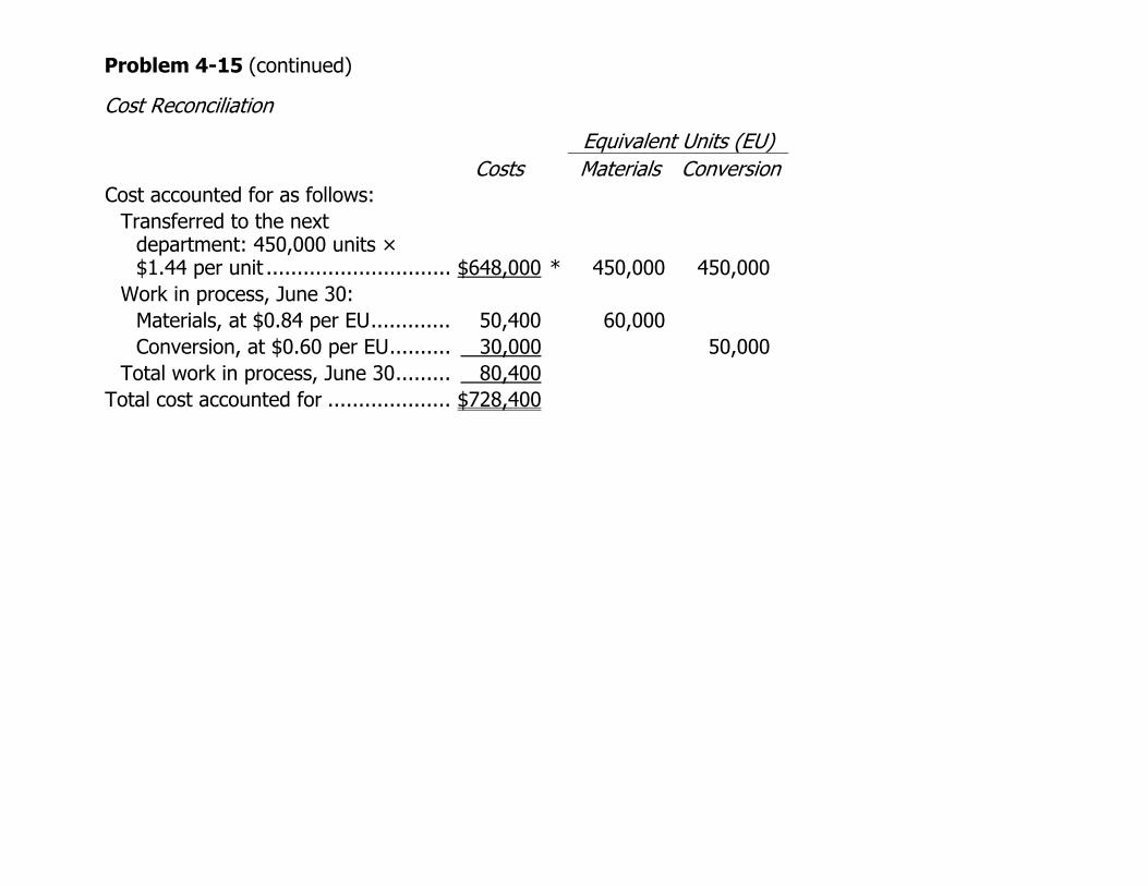
Cost Reconciliation
Equivalent Units (EU) Costs Materials ConversionCost accounted for as follows:
Transferred to the next department: 450,000 units × $1.44 per unit .............................. $648,000 * 450,000 450,000
Work in process, June 30: Materials, at $0.84 per EU............. 50,400 60,000 Conversion, at $0.60 per EU.......... 30,000 50,000
Total work in process, June 30......... 80,400 Total cost accounted for .................... $728,400

Problem 4-17 (45 minutes)
Weighted-Average Method 1., 2., and 3.
Quantity Schedule and Equivalent Units
Quantity Schedule
Pounds to be accounted for: Work in process, May 1
(materials 100% complete, conversion 90% complete)....... 70,000
Started into production............... 350,000Total pounds to be accounted for .. 420,000
Equivalent Units (EU) Materials ConversionPounds accounted for as follows:
Transferred to Molding* ................. 380,000 380,000 380,000Work in process, May 31
(materials 75% complete, conversion 25% complete)........... 40,000 30,000 10,000
Total pounds accounted for............... 420,000 410,000 390,000
*70,000 + 350,000 – 40,000 = 380,000. Costs per Equivalent Unit
Total Cost Materials Conversion
Whole Unit
Costs to be accounted for: Work in process, May 1 .... $122,000 86,000 $ 36,000 $

Cost added during the month .......................... 645,000 447,000 198,000
Total cost to be accounted for (a)............................. $767,000 $533,000 $234,000
Equivalent units (b) ............ 410,000 390,000 Cost per equivalent unit
(a) ÷ (b) ......................... $1.30 + $0.60 = $1.90

Problem 4-17 (continued)
Cost Reconciliation
Equivalent Units (EU) Costs Materials ConversionCost accounted for as follows:
Transferred to Molding: 380,000 units × $1.90 per unit......... $722,000 380,000 380,000
Work in process, May 31: Materials, at $1.30 per EU................ 39,000 30,000 Conversion, at $0.60 per EU............. 6,000 10,000
Total work in process ......................... 45,000 Total cost accounted for ....................... $767,000

Exercise 5-1 (45 minutes)
1. Units Shipped Shipping Expense High activity level.............. 8 $3,600 Low activity level .............. 2 1,500 Change ........................... 6 $2,100
Variable cost element:
Change in cost $2,100
= =$350 per unitChange in activity 6 units
Fixed cost element: Shipping expense at the high activity level .................... $3,600Less variable cost element ($350 per unit × 8 units) ...... 2,800Total fixed cost ........................................................... 800 $
The cost formula is $800 per month plus $350 per unit shipped or
Y = $800 + $350X,
where X is the number of units shipped. 2. a. See the scattergraph on the following page. b. (Note: Students’ answers will vary due to the imprecision and subjective nature of this method of
estimating variable and fixed costs.)
Total cost at 5 units shipped per month [a point falling on the line in (a)]........................................ $2,600
Less fixed cost element (intersection of the Y axis) .... 1,100 Variable cost element .............................................. $1,500
$1,500 ÷ 5 units = $300 per unit.
The cost formula is $1,100 per month plus $300 per unit shipped or
Y = $1,100 + 300X,

where X is the number of units shipped.

Exercise 5-1 (continued)
2. a. The scattergraph appears below:
0
500
1,000
1,500
2,000
2,500
3,000
3,500
4,000
0 1 2 3 4 5 6 7 8 9 10Units Shipped
Tota
l Shi
ppin
g Ex
pens
e
3. The cost of shipping units is likely to depend on the weight and volume of the units shipped and the distance traveled as well as on the number of units shipped. In addition, higher cost shipping might be necessary in to meet a deadline.

Exercise 5-3 (20 minutes)
1. X-rays Taken X-ray Costs High activity level (February) .......... 7,000 $29,000 Low activity level (June) ................. 3,000 17,000 Change ......................................... 4,000 $12,000
Variable cost per X-ray:
Change in cost $12,000
= =$3.00 pe X-rayChange in activity 4,000 X-rays
r
Fixed cost per month:
X-ray cost at the high activity level .......................... $29,000Less variable cost element:
7,000 X-rays × $3.00 per X-ray ............................. 21,000Total fixed cost ...................................................... 8,000 $
The cost formula is $8,000 per month plus $3.00 per X-ray taken or, in terms of the equation for a straight line:
Y = $8,000 + $3.00X
where X is the number of X-rays taken. 2. Expected X-ray costs when 4,600 X-rays are taken:
Variable cost: 4,600 X-rays × $3.00 per X-ray.............. $13,800 Fixed cost................................................................. 8,000 Total cost ................................................................. $21,800
Exercise 5-9 (20 minutes)
1. THE HAAKI SHOP, INC. Income Statement—Surfboard Department
For the Quarter Ended May 31
Sales.................................................................. $800,000 Less variable expenses: Cost of goods sold ($150 per surfboard ×
2,000 surfboards*)......................................... $300,000 Selling expenses ($50 per surfboard × 2,000
surfboards) ................................................... 100,000 Administrative expenses (25% × $160,000) ....... 40,000 440,000
Contribution margin ............................................ 360,000 Less fixed expenses:
Selling expenses............................................... 150,000 Administrative expenses.................................... 120,000 270,000
Net operating income .......................................... $ 90,000
*$800,000 sales ÷ $400 per surfboard = 2,000 surfboards. 2. Since 2,000 surfboards were sold and the contribution margin totaled $360,000 for the quarter, the
contribution of each surfboard toward fixed expenses and profits was $180 ($360,000 ÷ 2,000 surfboards = $180 per surfboard). Another way to compute the $180 is:
Selling price per surfboard.................... $400 Less variable expenses:
Cost per surfboard ............................ $150 Selling expenses ............................... 50 Administrative expenses
($40,000 ÷ 2,000 surfboards) ........
. 20 220 Contribution margin per surfboard ........ $180
Problem 5-12 (45 minutes)
1. HOUSE OF ORGANS, INC.
Income Statement For the Month Ended November 30
Sales (60 organs × $2,500 per organ) .................. $150,000
Less cost of goods sold
(60 organs × $1,500 per organ) ........................ 90,000
Gross margin ...................................................... 60,000 Less operating expenses:
Selling expenses:Advertising .................................................... $ 950
Delivery of organs
(60 organs × $60 per organ)........................ 3,600
Sales salaries and commissions
[$4,800 + (4% × $150,000)] ....................... 10,800 Utilities ......................................................... 650
Depreciation of sales facilities ......................... 5,000 Total selling expenses ....................................... 21,000 13,500
[$2,500 + (60 organs × $40 per organ)]....... 4,900
Administrative expenses: Executive salaries...........................................
Depreciation of office equipment.....................Clerical
900
Insurance...................................................... 700 Total administrative expenses ............................ 20,000 Total operating expenses ..................................... 41,000 Net operating income .......................................... 19,000 $
Problem 5-12 (continued)
2. HOUSE OF ORGANS, INC.
Total r
Income Statement For the Month Ended November 30
Pe Unit Sales (60 organs × $2,500 per organ) ................. $150,000 $2,500 Less variable expenses:
1,500
(60 organs × $60 per organ) ......................... Sales commissions (4% × $150,000) ................
Cost of goods sold (60 organs × $1,500 per organ).....................
Delivery of organs 90,000
3,600 60 6,000 100 Clerical (60 organs × $40 per organ) ................ 2,400 40 Total variable expenses ................................. 102,000 1,700 Contribution margin ........................................... 48,000 $ 800
Executive salaries ............................................
Less fixed expenses: Advertising......................................................
Sales salaries ..................................................950
4,800 650 Utilities ...........................................................
Depreciation of sales facilities........................... 5,000 13,500
Depreciation of office equipment ...................... 900 Clerical ........................................................... 2,500 Insurance ....................................................... 700
Total fixed expenses........................................... 29,000 Net operating income ......................................... $ 19,000 3. Fixed costs remain constant in total but vary on a per unit basis with changes in the activity level. For
example, as the activity level increases, fixed costs decrease on a per unit basis. Showing fixed costs

on a per unit basis on the income statement make them appear to be variable costs. That is, management might be misled into thinking that the per unit fixed costs would be the same regardless of how many pianos were sold during the month. For this reason, fixed costs should be shown only in totals on a contribution-type income statement.
Problem 5-14 (30 minutes)
1. a. 6 b. 11 c. 2
7
1d.e.
4
f. 10g. 3
h. i. 9
2. Without a knowledge of underlying cost behavior patterns, it would be difficult if not impossible for a
manager to properly analyze the firm’s cost structure. The reason is that all costs don’t behave in the same way. One cost might move in one direction as a result of a particular action, and another cost might move in an opposite direction. Unless the behavior pattern of each cost is clearly understood, the impact of a firm’s activities on its costs will not be known until after the activity has occurred.
Problem 5-15 (45 minutes)
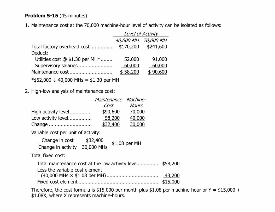
1. Maintenance cost at the 70,000 machine-hour level of activity can be isolated as follows:
Level of Activity 70,000 MH
ost @ $1.30 per MH*........ 52,000 91,000
40,000 MH$170,200Total factory overhead cost ...............
$241,600
Deduct:Utilities cSupervisory salaries ....................... 60,000 60,000
Maintenance cost ............................. $ 58,200 $ 90,600
*$52,000 ÷ 40,000 MHs = $1.30 per MH
Maintenance
Cost
2. High-low analysis of maintenance cost:
Machine-Hours
High activity level ................ $90,600 70,000Low activity level................. 58,200 40,000 Change .............................. $32,400 30,000
Variable cost per unit of activity:
Change in cost $32,400= =$1.08 per MH
Change in activity 30,000 MHs
Total fixed cost:
$58,200
Total maintenance cost at the low activity level..............Less the variable cost element
(40,000 MHs × $1.08 per MH) ................................... 43,200Fixed cost element ...................................................... $15,000
Therefore, the cost formula is $15,000 per month plus $1.08 per machine-hour or Y = $15,000 + $1.08X, where X represents machine-hours.
Problem 5-15 (continued)
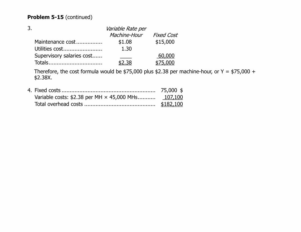
3.
Variable Rate per Machine-Hour
Fixed Cost
Maintenance cost ................. $1.08 $15,000 Utilities cost......................... 1.30
Supervisory salaries cost...... . 60,000 Totals.................................. $2.38 $75,000
Therefore, the cost formula would be $75,000 plus $2.38 per machine-hour, or Y = $75,000 + $2.38X.
4. Fixed costs ..........................................................
Variable costs: $2.38 per MH × 45,000 MHs...........75,000 $
107,100 $182,100 Total overhead costs ............................................
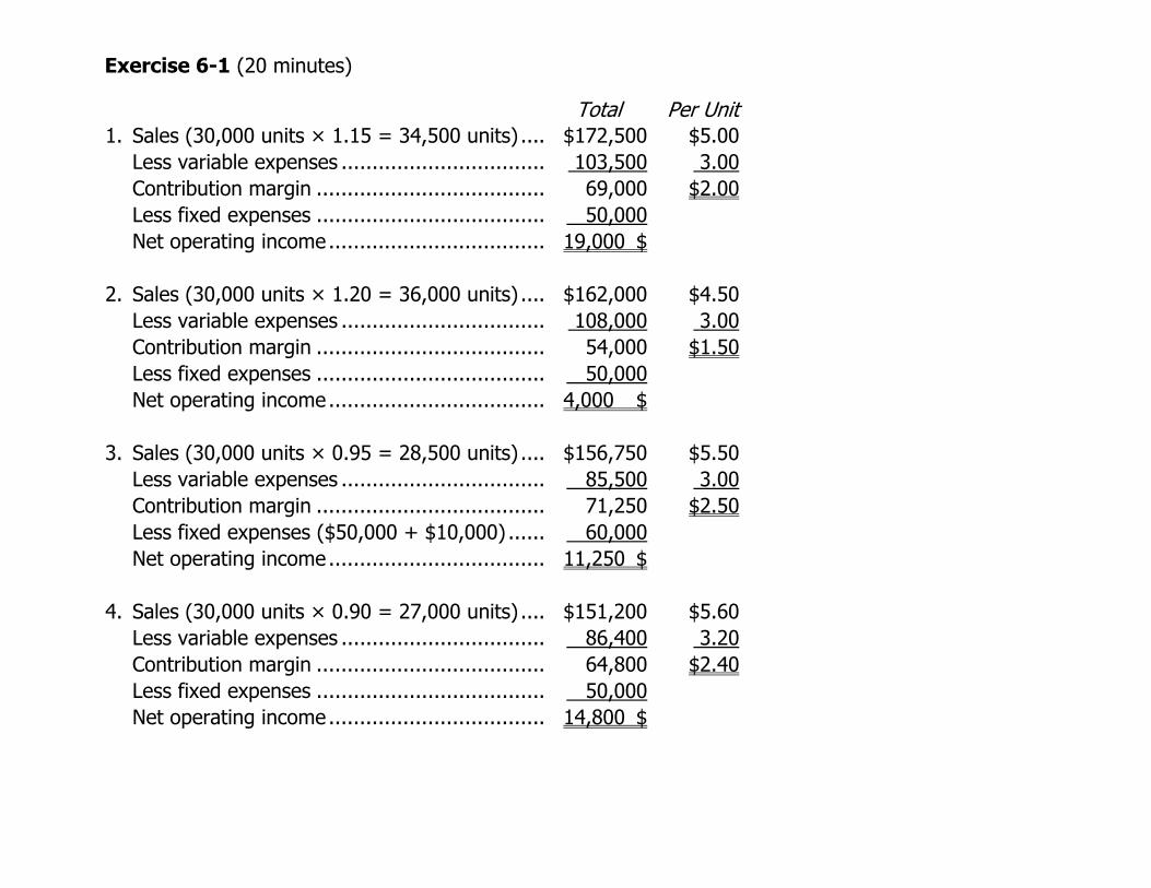
Exercise 6-1 (20 minutes)
Total Per Unit1. Sales (30,000 units × 1.15 = 34,500 units) .... $172,500 $5.00 Less variable expenses ................................. 103,500 3.00 Contribution margin ..................................... 69,000 $2.00 Less fixed expenses ..................................... 50,000 Net operating income................................... 19,000 $ 2. Sales (30,000 units × 1.20 = 36,000 units) .... $162,000 $4.50 Less variable expenses ................................. 108,000 3.00 Contribution margin ..................................... 54,000 $1.50 Less fixed expenses ..................................... 50,000 Net operating income................................... 4,000 $ 3. Sales (30,000 units × 0.95 = 28,500 units) .... $156,750 $5.50 Less variable expenses ................................. 85,500 3.00 Contribution margin ..................................... 71,250 $2.50 Less fixed expenses ($50,000 + $10,000) ...... 60,000 Net operating income................................... 11,250 $ 4. Sales (30,000 units × 0.90 = 27,000 units) .... $151,200 $5.60 Less variable expenses ................................. 86,400 3.20 Contribution margin ..................................... 64,800 $2.40 Less fixed expenses ..................................... 50,000 Net operating income................................... 14,800 $

Exercise 6-3 (30 minutes)
1.
Sales
$135,000 ÷ $27 per lantern
=
= Variable expenses + Fixed expenses + Profits $90Q = $63Q + $135,000 + $0
$27Q ==
$135,000 Q Q 5,000 lanterns, or at $90 per lantern, $450,000 in sales Alternative solution:
Fixed expensesBreak-even point = in unit sales Unit contribution margin
$135,000= = 5,000 lanterns,
$27 per lantern
or at $90 per lantern, $450,000 in sales 2. An increase in the variable expenses as a percentage of the selling price would result in a higher
break-even point. The reason is that if variable expenses increase as a percentage of sales, then the contribution margin will decrease as a percentage of sales. A lower CM ratio would mean that more lanterns would have to be sold to generate enough contribution margin to cover the fixed costs.

Exercise 6-3 (continued)
3. Present:
8,000 Lanterns Proposed:
10,000 Lanterns* Total
$720,00Per Unit Total Per Unit
$81Sales................................ $90 $810,000 ** Less variable expenses ...... 504,000 63 630,000 63
Contribution margin .......... 216,000 $27 180,000 $18 Less fixed expenses .......... 135,000 135,000 Net operating income........ 81,000 $ 45,000 $
4.
0
* **
8,000 lanterns × 1.25 = 10,000 lanterns $90 per lantern × 0.9 = $81 per lantern
As shown above, a 25% increase in volume is not enough to offset a 10% reduction in the selling price; thus, net operating income decreases.
Sales $81Q
= Variable expenses + Fixed expenses + Profits = $63Q + $135,000 + $72,000
$18QQ
==
$207,000 $207,000 ÷ $18 per lantern
Q 11,500 lanterns= Alternative solution:
Fixed expenses + Target profitUnit sales to attain = target profit Unit contribution margin
$135,000 + $72,000= = 11,500 lanterns
$18 per lantern

Exercise 6-4 (15 minutes)
1. Sales (30,000 doors) .............. $1,800,000 $60 Less variable expenses ........... 1,260,000 42
Contribution margin ............... 540,000 $18 Less fixed expenses ............... 450,000 Net operating income............. $ 90,000
Contribution marginDegree of operating = leverage Net operating income
$540,000= =6
$90,000
2. a. Sales of 37,500 doors represents an increase of 7,500 doors, or 25%, over present sales of 30,000 doors. Since the degree of operating leverage is 6, net operating income should increase by 6 times as much, or by 150% (6 × 25%).
135,000
b. Expected total dollar net operating income for the next year is:
Present net operating income.............................. 90,000 $ Expected increase in net operating income next
year (150% × $90,000) ...................................Total expected net operating income ...................
$225,000
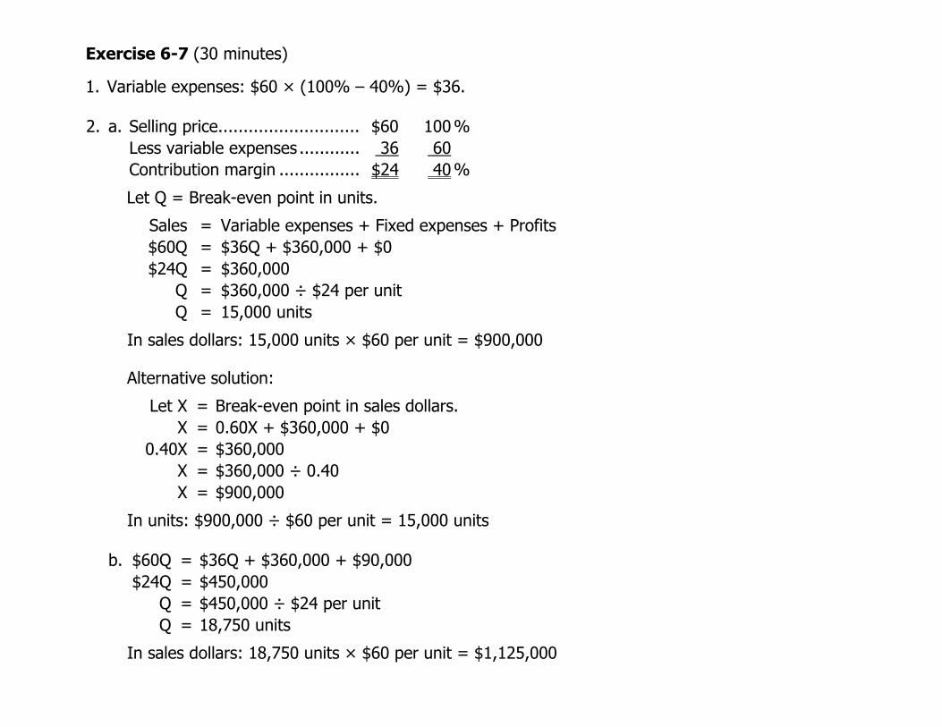
Exercise 6-7 (30 minutes)
. 100 %
1. Variable expenses: $60 × (100% – 40%) = $36. 2 a. Selling price............................ $60 Less variable expenses ............ 36 60 Contribution margin ................ $24 40%
Let Q = Break-even point in units.
Variable expenses + Fixed expenses + Profits
Alternative solution:
Let X Break-even point in sales dollars. X 0.60X + $360,000 + $0
0.40X = $360,000 X =
In units: $900,000 ÷ $60 per unit = 15,000 units
= $36Q + $360,000 + $90,000 = $450,000
$450,000 ÷ $24 per unit 18,750 units
Sales = = $60Q $36Q + $360,000 + $0
$24Q = $360,000Q = $360,000 ÷ $24 per unit
Q = 15,000 units
In sales dollars: 15,000 units × $60 per unit = $900,000
= =
$360,000 ÷ 0.40 $900,000 X =
b.
$60Q $24Q
Q Q
= =
In sales dollars: 18,750 units × $60 per unit = $1,125,000

Exercise 6–7 (continued)
Alternative solution:
X = 0.60X + $360,000 + $90,000 0.40X = $450,000
X $450,000 ÷ 0.40 =
In units: $1,125,000 ÷ $60 per unit = 18,750 units c. The company’s new cost/revenue relationships will be:
Selling price ........................................
= X $1,125,000
. $60 100% Less variable expenses ($36 – $3) ......... 33 55 Contribution margin.............................. $27 45%
= =
Alternative solution:
=
X $360,000 ÷ 0.45
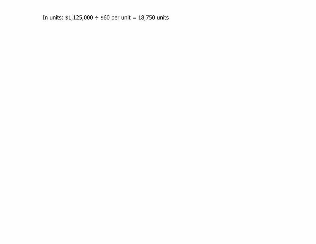
In units: $800,000 ÷ $60 per unit = 13,333 units (rounded)
$60Q $33Q + $360,000 + $0 $27Q $360,000
Q = Q =
$360,000 ÷ $27 per unit 13,333 units (rounded).
In sales dollars: 13,333 units × $60 per unit = $800,000 (rounded)
X 0.45X =
0.55X + $360,000 + $0 $360,000
= X = $800,000

Exercise 6–7 (continued)
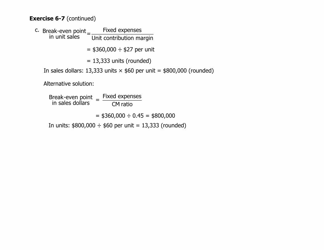
3. a. Fixed expensesBreak-even point = in unit sales Unit contribution margin
= $360,000 ÷ $24 per unit = 15,000 units
In sales dollars: 15,000 units × $60 per unit = $900,000 Alternative solution:
Fixed expensesBreak-even point = in sales dollars CM ratio
= $360,000 ÷ 0.40 = $900,000
In units: $900,000 ÷ $60 per unit = 15,000 units
b. Fixed expenses + Target profitUnit sales to attain= target profit Unit contribution margin
= ($360,000 + $90,000) ÷ $24 per unit
= 18,750 units
In sales dollars: 18,750 units × $60 per unit = $1,125,000 Alternative solution:
Fixed expenses + Target profitDollar sales to attain= target profit CM ratio
= ($360,000 + $90,000) ÷ 0.40
= $1,125,000
In units: $1,125,000 ÷ $60 per unit = 18,750 units
Exercise 6-7 (continued)
c. Fixed expensesBreak-even point=in unit sales Unit contribution margin
= $360,000 ÷ $27 per unit
= 13,333 units (rounded)
In sales dollars: 13,333 units × $60 per unit = $800,000 (rounded)
Alternative solution:
Fixed expensesBreak-even point = in sales dollars CM ratio
= $360,000 ÷ 0.45 = $800,000
In units: $800,000 ÷ $60 per unit = 13,333 (rounded)

Problem 6-9 (60 minutes)
Total Per Unit Percentage Sales (13,500 units) ......... $270,000 %
1. The CM ratio is 30%.
$20 100Less variable expenses ..... 189,000 14 70Contribution margin.......... 81,000 $ 6 $ 30%
The break-even point is:
Sales = Variable expenses + Fixed expenses + Profits = =
Q = $90,000 ÷ $6 per unit Q =
Alternative solution:
$20Q $ 6Q
$14Q + $90,000 + $0 $90,000
15,000 units
15,000 units × $20 per unit = $300,000 in sales
Fixed expensesBreak-even point = in unit sales Unit contribution margin
$90,000= = 15,000 units
$6 per unit
Fixed expensesBreak-even point = in sales dollars CM ratio
$90,000= = $300,000 in sales
0.30
2.
Incremental contribution margin: $70,000 increased sales × 30% CM ratio............. $21,000
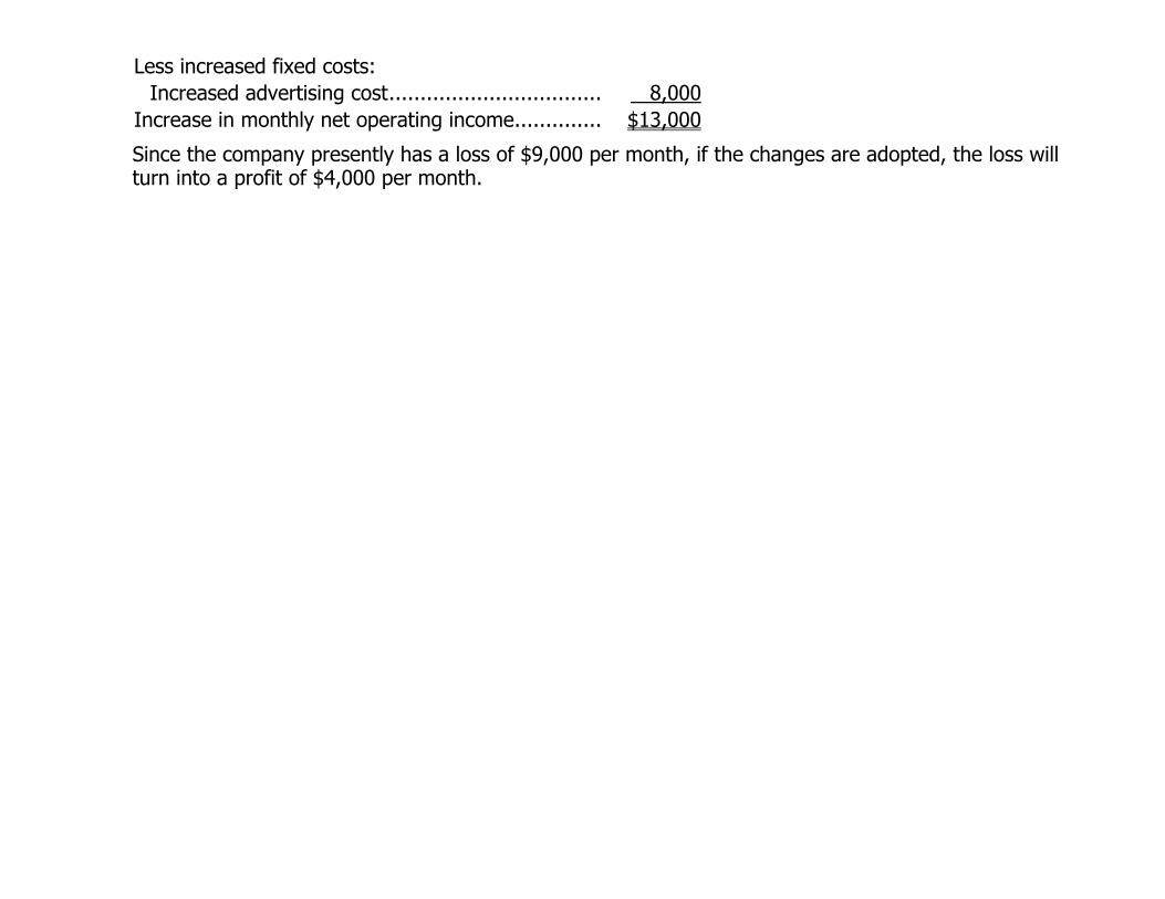
Less increased fixed costs: 8,000Increased advertising cost.................................. Increase in monthly net operating income.............. $13,000
Since the company presently has a loss of $9,000 per month, if the changes are adopted, the loss will turn into a profit of $4,000 per month.

Problem 6-9 (continued)
3.
(27,000 units × $14 per unit) ........................
Sales (27,000 units × $18 per unit*) ................Less variable expenses
$486,000
378,000Contribution margin ........................................ 108,000 Less fixed expenses ($90,000 + $35,000) ......... 125,000
Net operating loss........................................... $(17,000)
*$20 – ($20 × 0.10) = $18 4. Sales
$ 20Q = =
$5.40Q Q = Q =
Alternative solution:
Variable expenses + Fixed expenses + Profits $14.60Q* + $90,000 + $4,500
= $94,500 $94,500 ÷ $5.40 per unit
17,500 units *$14.00 + $0.60 = $14.60.
Fixed expenses + Target profitUnit sales to attain = target profit CM per unit
$90,000 + $4,500=
$5.40 per unit**
= 17,500 units
**$6.00 – $0.60 = $5.40. 5. a. The new CM ratio would be:
Per Unit Percentage

Sales ...........................................Less variable expenses .................
$20 100 % 7 35
Contribution margin...................... $13 65%

Problem 6-9 (continued)
The new break-even point would be:
Fixed expensesBreak-even point = in unit sales Unit contribution margin
$208,000= = 16,000 units
$13 per unit
Fixed expensesBreak-even point = in sales dollars CM ratio
$208,000= = $320,000 in sales
0.65
b. Comparative income statements follow:
Not Automated Automated
Total
$400,000Per Unit % Total
$400,000 Per Unit %
Sales (20,000 units) ...... $20 100 $20 100Less variable expenses .. 280,000 14 70 140,000 7 35Contribution margin....... 120,000 $ 6 30 260,000 $13 65
90,000 208,000 Net operating income .... 30,000 $ 52,000 $
Less fixed expenses.......
Problem 6-9 (continued)
c. Whether or not one would recommend that the company automate its operations depends on how much risk he or she is willing to take, and depends heavily on prospects for future sales. The proposed changes would increase the company’s fixed costs and its break-even point. However, the changes would also increase the company’s CM ratio (from 30% to 65%). The higher CM ratio means that once the break-even point is reached, profits will increase more rapidly than at present. If 20,000 units are sold next month, for example, the higher CM ratio will generate $22,000 more in profits than if no changes are made.
The greatest risk of automating is that future sales may drop back down to present levels (only 13,500 units per month), and as a result, losses will be even larger than at present due to the company’s greater fixed costs. (Note the problem states that sales are erratic from month to month.) In sum, the proposed changes will help the company if sales continue to trend upward in future months; the changes will hurt the company if sales drop back down to or near present levels.
=
$118,000 ÷ $7 per unit =
Note to the Instructor: Although it is not asked for in the problem, if time permits you may want to compute the point of indifference between the two alternatives in terms of units sold; i.e., the point where profits will be the same under either alternative. At this point, total revenue will be the same; hence, we include only costs in our equation:
Let Q Point of indifference in units sold $14Q + $90,000
$7Q = $7Q + $208,000 = =
$118,000 Q Q 16,857 units (rounded)
If more than 16,857 units are sold, the proposed plan will yield the greatest profit; if less than 16,857 units are sold, the present plan will yield the greatest profit (or the least loss).

Problem 6-11 (30 minutes)
Product 1. Mirrors Sinks Vanities Total
Percentage of total
sales .......................... 32% 28%
40% 100%Sales.............................$160,000 100 100 % 100% $200,000 % $140,000 % $500,000 100
Less variable expenses ... 48,000 30 160,000 80 77,000 55 285,000 57 Contribution margin .......$112,000 70% $ 40,000 20% $ 63,000 45% 215,000 43%* Less fixed expenses ....... 223,600
(loss).........................Net operating income
. $( 8,600)
*$215,000 ÷ $500,000 = 43%.

Problem 6-11 (continued)
2. Break-even sales:
Fixed expensesBreak-even point = in total dollar sales CM ratio
$223,600= = $520,000 in sales
0.43
3. Memo to the president:
Although the company met its sales budget of $500,000 for the month, the mix of products sold changed substantially from that budgeted. This is the reason the budgeted net operating income was not met, and the reason the break-even sales were greater than budgeted. The company’s sales mix was planned at 48% Sinks, 20% Mirrors, and 32% Vanities. The actual sales mix was 32% Sinks, 40% Mirrors, and 28% Vanities.
As shown by these data, sales shifted away from Sinks, which provides our greatest contribution per dollar of sales, and shifted strongly toward Mirrors, which provides our least contribution per dollar of sales. Consequently, although the company met its budgeted level of sales, these sales provided considerably less contribution margin than we had planned, with a resulting decrease in net operating income. Notice from the attached statements that the company’s overall CM ratio was only 43%, as compared to a planned CM ratio of 52%. This also explains why the break-even point was higher than planned. With less average contribution margin per dollar of sales, a greater level of sales had to be achieved to provide sufficient contribution margin to cover fixed costs.
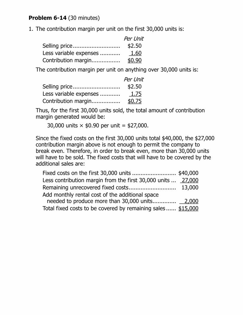
Problem 6-14 (30 minutes)
1. The contribution margin per unit on the first 30,000 units is:
Per Unit
Selling price............................ $2.50 Less variable expenses ............ 1.60 Contribution margin................. $0.90
The contribution margin per unit on anything over 30,000 units is:
r Selling price............................ $2.50 Less variable expenses ............
Pe Unit
1.75 Contribution margin................. $0.75
Thus, for the first 30,000 units sold, the total amount of contribution margin generated would be:
Since the fixed costs on the first 30,000 units total $40,000, the $27,000 contribution margin above is not enough to permit the company to break even. Therefore, in order to break even, more than 30,000 units will have to be sold. The fixed costs that will have to be covered by the additional sales are:
30,000 units × $0.90 per unit = $27,000.
Fixed costs on the first 30,000 units .......................... $40,000Less contribution margin from the first 30,000 units ... 27,000Remaining unrecovered fixed costs............................ 13,000Add monthly rental cost of the additional space
needed to produce more than 30,000 units.............. 2,000Total fixed costs to be covered by remaining sales ...... $15,000

Problem 6-14 (continued)
The additional sales of units required to cover these fixed costs would be:
Therefore, a total of 50,000 units (30,000 + 20,000) must be sold for the company to break even. This number of units would equal total sales of:
50,000 units × $2.50 per unit = $125,000 in total sales. 2.
The desired monthly profit would be:
25% × ($40,000 + $2,000) = $10,500
Thus,
Therefore, the company must sell 17,500 units above the break-even point to earn a profit of $10,500 each month. These units, added to the 50,000 units required to break even, would equal total sales of 67,500 units each month.
Total remaining fixed costs $15,000=
Unit contribution margin on added units $0.75 per unit
=20,000 units
Target profit $9,000= =12,000 units
Unit contribution margin $0.75 per unit
Thus, the company must sell 12,000 units above the break-even point to earn a profit of $9,000 each month. These units, added to the 50,000 units required to break even, would equal total sales of 62,000 units each month to reach the target profit figure.
3. If a bonus of $0.15 per unit is paid for each unit sold in excess of the
break-even point, then the contribution margin on these units would drop from $0.75 to only $0.60 per unit.
Target profit $10,500= =17,500 units
Unit contribution margin $0.60 per unit

Problem 6-15 (30 minutes)
1. The numbered components are as follows:
Dollars of revenue and costs.
(3)
(9) line.
(1) (2) Volume of output, expressed in units,% of capacity, sales,
or some other measure of activity. Total expense line.
(4) Variable expense area. (5) Fixed expense area. (6) Break-even point. (7) Loss area. (8) Profit area.
Revenue

Problem 6-15 (continued)
2. a. Line 3:
b.
Break-even point:
d. Line 3:
ard and have a flatter slope.
Line 9:
Remain unchanged. Line 9: Have a flatter slope.
Break-even point: Increase.
Line 3: Have a steeper slope. Line 9: Remain unchanged. Increase.
c. Line 3: Shift downward. Line 9: Remain unchanged. Break-even point: Decrease.
Remain unchanged. Line 9: Remain unchanged. Break-even point: Remain unchanged.
e. Line 3: Shift upw Line 9: Remain unchanged.
Break-even point: Probably change, but the direction is
uncertain.
f. Line 3: Have a flatter slope. Have a flatter slope.
Break-even point:
Remain unchanged in terms of units;
decrease in terms of total dollars of sales.
g. Line 3: Shift upward. Line 9: Remain unchanged. Break-even point: Increase.
h. Line 3: Shift downward and have a steeper slope. Line 9: Remain unchanged.
Break-even point:
Probably change, but the direction is
uncertain.
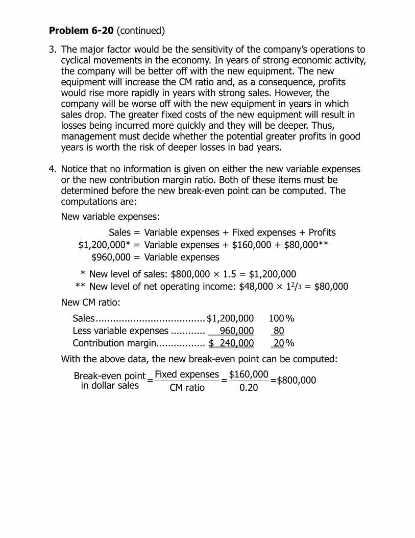
Problem 6-20 (continued)
3. The major factor would be the sensitivity of the company’s operations to cyclical movements in the economy. In years of strong economic activity, the company will be better off with the new equipment. The new equipment will increase the CM ratio and, as a consequence, profits would rise more rapidly in years with strong sales. However, the company will be worse off with the new equipment in years in which sales drop. The greater fixed costs of the new equipment will result in losses being incurred more quickly and they will be deeper. Thus, management must decide whether the potential greater profits in good years is worth the risk of deeper losses in bad years.
4. Notice that no information is given on either the new variable expenses
or the new contribution margin ratio. Both of these items must be determined before the new break-even point can be computed. The computations are:
New variable expenses:
Sales = Variable expenses + Fixed expenses + Profits $1,200,000* = Variable expenses + $160,000 + $80,000**
$960,000
Sales...................................... 100
= Variable expenses
* New level of sales: $800,000 × 1.5 = $1,200,000 ** New level of net operating income: $48,000 × 12/3 = $80,000
New CM ratio:
$1,200,000 % Less variable expenses ............ 960,000 80 Contribution margin................. $ 240,000 20%
With the above data, the new break-even point can be computed:
Fixed expenses $160,000Break-even point= = =$800,000in dollar sales CM ratio 0.20

Problem 6-20 (continued)
The greatest risk with the new method is that the president’s estimates of increases in sales and net operating income will not materialize and that sales will remain at their present level. Note that the present level of sales is $800,000, which is just equal to the break-even level of sales under the new marketing method. Thus, if the new method is adopted and sales remain unchanged, profits will drop from the current level of $48,000 per month to zero.
Although not required in the problem, you may wish to work out the level of sales needed under the new method to generate at least $48,000 in profits each month. The computations are:
Fixed expenses + Target profitDollar sales to attain= target profit CM ratio
$160,000 + $48,000=
0.20
= $1,040,000 in sales each month
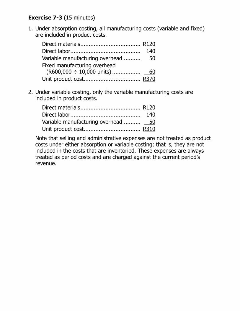
Exercise 7-3 (15 minutes)
1. Under absorption costing, all manufacturing costs (variable and fixed) are included in product costs.
Direct materials.................................... R120Direct labor.......................................... 140Variable manufacturing overhead .......... 50Fixed manufacturing overhead
(R600,000 ÷ 10,000 units) ................. 60Unit product cost.................................. R370
2. Under variable costing, only the variable manufacturing costs are
included in product costs.
Direct materials.................................... R120Direct labor.......................................... 140Variable manufacturing overhead .......... 50Unit product cost.................................. R310
Note that selling and administrative expenses are not treated as product costs under either absorption or variable costing; that is, they are not included in the costs that are inventoried. These expenses are always treated as period costs and are charged against the current period’s revenue.

Exercise 7-7 (20 minutes)
1. The company is using variable costing. The computations are:
Va iable Costing
r
$10 $10
Variable manufacturing overhead ..... 2
Absorption Costing
Direct materials...............................Direct labor..................................... 5 5
2 Fixed manufacturing overhead
($90,000 ÷ 30,000 units) .............. — 3 Unit product cost............................. $17 $20 Total cost, 5,000 units ..................... $85,000 $100,000
2. a. No, the $85,000 figure is not the correct figure to use, since variable
costing is not generally accepted for external reporting purposes or for tax purposes.
b. The finished goods inventory account should be stated at $100,000,
which represents the absorption cost to manufacture the 5,000 unsold units. Thus, the account should be increased by $15,000 for external reporting purposes. This $15,000 consists of the amount of fixed manufacturing overhead cost that is allocated to the 5,000 unsold units under absorption costing:
5,000 units × $3 per unit fixed manufacturing overhead cost = $15,000

Problem 7-9 (45 minutes)
1. a. The unit product cost under absorption costing:
$15 Direct labor......................................................Direct materials................................................
7 Variable manufacturing overhead ...................... 2 Fixed manufacturing overhead
(640,000 ÷ 40,000 units) ............................... 16 Unit product cost.............................................. $40
b. The absorption costing income statement follows:
Sales (35,000 units × $60 per unit) ........... $2,100,000 Less cost of goods sold: Beginning inventory ............................... $ 0
Add cost of goods manufactured
(40,000 units × $40 per unit) .............. 1,600,000 Goods available for sale ......................... 1,600,000
Less ending inventory
(5,000 units × $40 per unit) ................ 200,000 1,400,000 Gross margin ........................................... 700,000 Less selling and administrative expenses.... 630,000* Net operating income ............................... $ 70,000
*(35,000 units × $2 per unit) + $560,000 = $630,000. 2. a. The unit product cost under variable costing:
Direct materials............................................... $15 Direct labor..................................................... 7 Variable manufacturing overhead ..................... 2 Unit product cost............................................. $24

Problem 7-9 (continued)
b. The variable costing income statement follows:
Sales (35,000 units × $60 per unit) ................ $2,100,000Less variable expenses:
Variable cost of goods sold: Beginning inventory.................................. $ 0 Add variable manufacturing costs
(40,000 units × $24 per unit) ................. 960,000 Goods available for sale ............................Less ending inventory
(5,000 units × $24 per unit) ...................
960,000
120,000 Variable cost of goods sold .......................... 840,000 Variable selling expense
(35,000 units × $2 per unit) ..................... 70,000 910,000Contribution margin.......................................Less fixed expenses:
Fixed selling and administrative expense ......
1,190,000
Fixed manufacturing overhead..................... 640,000 560,000 1,200,000
Net operating loss ......................................... $ (10,000) 3. The difference in the ending inventory relates to a difference in the
handling of fixed manufacturing overhead costs. Under variable costing, these costs have been expensed in full as period costs. Under absorption costing, these costs have been added to units of product at the rate of $16 per unit ($640,000 ÷ 40,000 units produced = $16 per unit). Thus, under absorption costing a portion of the $640,000 fixed manufacturing overhead cost of the month has been added to the inventory account rather than expensed on the income statement:
Added to the ending inventory (5,000 units × $16 per unit) ........................................ 80,000 $
Expensed as part of cost of goods sold (35,000 units × $16 per unit) ...................................... 560,000
Total fixed manufacturing overhead cost for the month .... $640,000
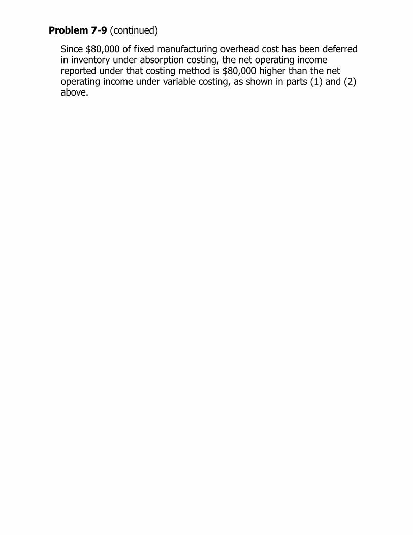
Problem 7-9 (continued)
Since $80,000 of fixed manufacturing overhead cost has been deferred in inventory under absorption costing, the net operating income reported under that costing method is $80,000 higher than the net operating income under variable costing, as shown in parts (1) and (2) above.

Problem 8-13 (45 minutes)
1. a. When direct labor-hours are used to apply overhead cost to products, the company’s predetermined overhead rate would be:
Manufacturing overhead costPredeterminedoverhead rate Direct labor hours
$1,480,000$74 per DLH
20,000 DLHs
=
= =
Model b. XR7
Direct labor: $20 per hour × 0.2 DLH, 0.4 DLH ............. 8.00
ZD5Direct materials.......................................... $35.00 $25.00
4.00
Manufacturing overhead: $74 per hour × 0.2 DLH, 0.4 DLH ............. 14.80 29.60
Total unit product cost................................ $53.80 $62.60
2. a. Predetermined overhead rates for the activity cost pools:
Activity Cost Pool
(a) Total Cost
(b) Total Activity
(a) ÷ (b) Activity Rate
Machine setups....... $180,000 250 setups $720 per setup Special milling ........ $300,000 1,000 MHs $300 per MH
General factory....... $1,000,000 20,000 DLHs $50 per DLH
The manufacturing overhead cost that would be applied to each model can be computed as follows:
Model XR7 ZD5
$ 72,000Special milling:
$300 per MH × 1,000 MHs, 0 MHs............... 0
Machine setups: $720 per setup × 150 setups, 100 setups .... $108,000
300,000
General factory: $50 per DLH × 4,000 DLHs, 16,000 DLHs .... 200,000 800,000
Total manufacturing overhead cost applied..... $872,000$608,000
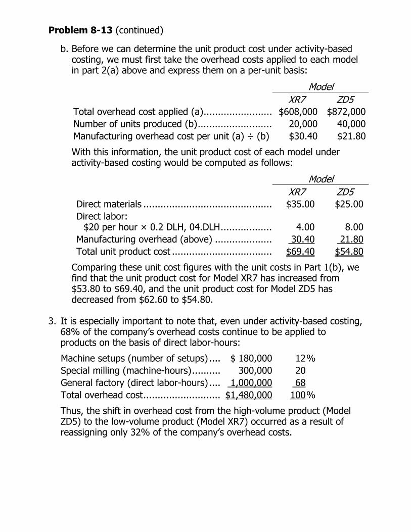
Problem 8-13 (continued)
b. Before we can determine the unit product cost under activity-based costing, we must first take the overhead costs applied to each model in part 2(a) above and express them on a per-unit basis:
Model XR7 ZD5
With this information, the unit product cost of each model under activity-based costing would be computed as follows:
Total overhead cost applied (a)........................ $608,000 $872,000Number of units produced (b).......................... 20,000 40,000
Manufacturing overhead cost per unit (a) ÷ (b) $30.40 $21.80
Model
Direct materials .............................................Direct labor:
$20 per hour × 0.2 DLH, 04.DLH.................. 8.00
XR7 ZD5 $35.00 $25.00
4.00 Manufacturing overhead (above) .................... 30.40 21.80 Total unit product cost ................................... $69.40 $54.80
Comparing these unit cost figures with the unit costs in Part 1(b), we find that the unit product cost for Model XR7 has increased from $53.80 to $69.40, and the unit product cost for Model ZD5 has decreased from $62.60 to $54.80.
20
3. It is especially important to note that, even under activity-based costing, 68% of the company’s overhead costs continue to be applied to products on the basis of direct labor-hours:
Machine setups (number of setups) .... $ 180,000 12% Special milling (machine-hours).......... 300,000 General factory (direct labor-hours) .... 1,000,000 68 Total overhead cost........................... $1,480,000 100%
Thus, the shift in overhead cost from the high-volume product (Model ZD5) to the low-volume product (Model XR7) occurred as a result of reassigning only 32% of the company’s overhead costs.

Problem 8-13 (continued)
The increase in unit product cost for Model XR7 can be explained as follows: First, where possible, overhead costs have been traced to the products rather than being lumped together and spread uniformly over production. Therefore, the special milling costs, which are traceable to Model XR7, have all been assigned to Model XR7 and none assigned to Model ZD5 under the activity-based costing approach. It is common in industry to have some products that require special handling or special milling of some type. This is especially true in modern factories that produce a variety of products. Activity-based costing provides a vehicle for assigning these costs to the appropriate products.
Second, the costs associated with the batch-level activity (machine setups) have also been assigned to the specific products to which they relate. These costs have been assigned according to the number of setups completed for each product. However, since a batch-level activity is involved, another factor affecting unit costs comes into play. That factor is batch size. Some products are produced in large batches and some are produced in small batches. The smaller the batch, the higher the per unit cost of the batch activity. In the case at hand, the data can be analyzed as shown below.
Number of units processed per setup (20,000 units ÷ 150 setups) ....................... 133.33 (b)
400 (b)
Model XR7: Cost to complete one setup [see 2(a)] ........... $720 (a)
Setup cost per unit (a) ÷ (b) ......................... $5.40 Model ZD5:
Cost to complete one setup (above)............... $720 (a) Number of units processed per setup
(40,000 units ÷ 100 setups) ....................... Setup cost per unit (a) ÷ (b) ......................... $1.80

Problem 8-13 (continued)
Thus, the cost per unit for setups is three times as great for Model XR7, the low-volume product, as it is for Model ZD5, the high-volume product. Such differences in cost are obscured when direct labor-hours (or any other volume measure) is used as a basis for applying overhead cost to products.
In sum, overhead cost has shifted from the high-volume product to the low-volume product as a result of more appropriately assigning some costs to the products on the basis of the activities involved, rather than on the basis of direct labor-hours.
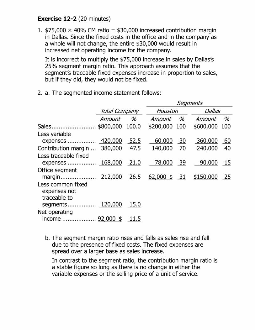
Exercise 12-2 (20 minutes)
1. $75,000 × 40% CM ratio = $30,000 increased contribution margin in Dallas. Since the fixed costs in the office and in the company as a whole will not change, the entire $30,000 would result in increased net operating income for the company.
It is incorrect to multiply the $75,000 increase in sales by Dallas’s 25% segment margin ratio. This approach assumes that the segment’s traceable fixed expenses increase in proportion to sales, but if they did, they would not be fixed.
2. a. The segmented income statement follows:
Segments Total Company Houston Dallas
Amount % % 100
Amount % Amount Sales......................... $800,000 100.0 $200,000 $600,000 100Less variable
expenses ................ 420,000 52.5 60,000 30
360,000 60Contribution margin ... 380,000 47.5 140,000 70 240,000 40Less traceable fixed
expenses ................ 168,000 21.0 78,000 39
90,000 15Office segment
margin.................... 212,000 26.5 62,000 $ 31
$150,000 25Less common fixed
expenses not traceable to segments................ 120,000 15.0
Net operating income ................... 92,000 $ 11.5
b. The segment margin ratio rises and falls as sales rise and fall due to the presence of fixed costs. The fixed expenses are spread over a larger base as sales increase.
In contrast to the segment ratio, the contribution margin ratio is a stable figure so long as there is no change in either the variable expenses or the selling price of a unit of service.

Exercise 12-3 (15 minutes)
1. The company should focus its campaign on Landscaping Clients. The computations are:
Construction
Clients Landscaping
Clients Increased sales......................................... $70,000 $60,000 Market CM ratio ........................................ × 35% × 50% Incremental contribution margin ................ 24,500 30,000 Less cost of the campaign ......................... 8,000 8,000 Increased segment margin and net
operating income for the company as a whole .................................................... $16,500 $22,000
2. The $90,000 in traceable fixed expenses in Exercise 12-2 is now
partly traceable and partly common. When we segment Dallas by market, only $72,000 remains a traceable fixed expense. This amount represents costs such as advertising and salaries that arise because of the existence of the construction and landscaping market segments. The remaining $18,000 ($90,000 – $72,000) becomes a common cost when Dallas is segmented by market. This amount would include such costs as the salary of the manager of the Dallas office that could not be avoided by eliminating either of the two market segments.
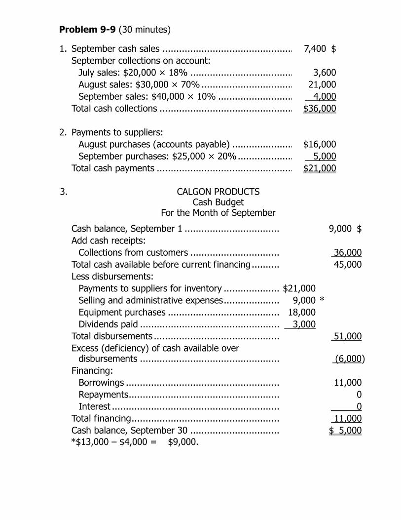
Problem 9-9 (30 minutes)
1. September cash sales ............................................... 7,400 $ September collections on account: July sales: $20,000 × 18% ..................................... 3,600 August sales: $30,000 × 70%................................. 21,000 September sales: $40,000 × 10% ........................... 4,000 Total cash collections ................................................ $36,000 2. Payments to suppliers: August purchases (accounts payable) ...................... $16,000 September purchases: $25,000 × 20%.................... 5,000 Total cash payments ................................................. $21,000
Cash balance, September 1 ..................................
3. CALGON PRODUCTS Cash Budget
For the Month of September
. 9,000 $ Add cash receipts:
Collections from customers ................................. 36,000 Total cash available before current financing...........
Less disbursements: 45,000
Payments to suppliers for inventory .....................$21,000 Selling and administrative expenses..................... 9,000 * Equipment purchases ......................................... 18,000 Dividends paid ................................................... 3,000 Total disbursements .............................................. 51,000
Excess (deficiency) of cash available over disbursements ................................................... (6,000)
Financing: Borrowings ........................................................ 11,000 Repayments....................................................... 0 Interest ............................................................. 0Total financing...................................................... 11,000
Cash balance, September 30 ................................. $ 5,000 *$13,000 – $4,000 = $9,000.

Problem 9-19 (120 minutes)
1. Schedule of expected cash collections:
Total Cash sales ............................... April May June
$14,000 $17,000 $18,000 49,000 $Credit sales ............................. 48,000 56,000 68,000 172,000Total collections ....................... $62,000 $73,000 $86,000 $221,000
2. a. Inventory purchases budget:
April $147,000
May June Total Budgeted cost of goods sold..... $42,000 $51,000 $54,000 Add desired ending inventory*.. 15,300 16,200 9,000 9,000Total needs ............................. 57,300 67,200 63,000 156,000Less beginning inventory.......... 12,600 15,300 16,200 12,600Required purchases ................. $44,700 $51,900 $46,800 $143,400
b. Schedule of cash disbursements for purchases:
April May For March purchases................ $18,300
51,900For June purchases..................
*At April 30: $51,000 × 30% = $15,300. At June 30: $50,000 July sales × 60% × 30% = $9,000.
June Total $18,300
For April purchases .................. 22,350 $22,350 44,700For May purchases................... 25,950 $25,950
23,400 23,400Total cash disbursements ......... $40,650 $48,300 $49,350 $138,300

Problem 9-19 (continued)
Salaries and wages ...................... 7,500 $
6,000 6,000 6,000 18,000
3. Schedule of cash disbursements for operating expenses:
April May June Total 7,500 $ 7,500 $ $22,500
Shipping ..................................... 4,200 5,100 5,400 14,700Advertising ..................................Other expenses ........................... 2,800 3,400 3,600 9,800Total cash disbursements for
operating expenses ................... $20,500 $22,000 $22,500 $65,000
May Cash balance, beginning............... 9,000 $
4. Cash budget: April June Total
8,350 $ 8,050 $ $ 9,000 Add cash collections..................... 62,000 73,000 86,000 221,000
Total cash available ................... 71,000 81,350 94,050 230,000 Less disbursements:
48,300 49,350 138,300 For operating expenses.............. 22,000 22,500 65,000 For equipment purchases...........For dividends ............................
For inventory purchases............. 40,650 20,500 11,500 3,000 0 14,500
0 0 3,500 3,500 Total disbursements ..................... 72,650 73,300 75,350 221,300 Excess (deficiency) of cash........... (1,650) 8,050 18,700 8,700
0 Repayments.............................. 0
Financing: Borrowings ............................... 10,000 0 10,000
0 (10,000) (10,000)Interest* .................................. 0 0 (300) (300)
Total financing............................. 10,000 0 (10,300) (300)Cash balance, ending ................... 8,350 $ 8,050 $ 8,400 $ $ 8,400
* $10,000 × 12% × 3/12 = $300.

Problem 9-19 (continued)
5. Income Statement:
NORDIC COMPANY
For the Quarter Ended June 30
Sales.........................................................
Income Statement
$245,000 Less cost of goods sold:
Beginning inventory (given) ..................... 12,600 $ Add purchases (Part 2) ............................ 143,400 Goods available for sale ........................... 156,000 Ending inventory (Part 2) ......................... 9,000 147,000
Gross margin ............................................. 98,000
22,500 Shipping (Part 3) ..................................... 14,700 Advertising (Part 3) .................................Depreciation ...........................................
Less operating expenses: Salaries and wages (Part 3)......................
18,000 6,000
Other expenses (Part 3)........................... 9,800 71,000 Net operating income................................. 27,000 Less interest expense (Part 4)..................... 300 Net income................................................ 26,700 $

Problem 9-19 (continued)
NORDIC COMPANY Balance Sheet
Assets
Cash (Part 4) ................................................................. $ 8,400Accounts receivable (80% × $90,000) .............................
6. Balance sheet:
June 30
Current assets:
72,000Inventory (Part 2)........................................................... 9,000
Total current assets........................................................... 89,400Buildings and equipment, net
($214,100 + $14,500 – $6,000) ...................................... 222,600Total assets ...................................................................... $312,000
Liabilities and Equity
Current liabilities: Accounts payable (Part 2: 50% × $46,800) .... 23,400 $
Stockholders’ equity:
Capital stock ................................................ $190,000 Retained earnings*....................................... 98,600 288,600
Total liabilities and equity ................................ $312,000
* Retained earnings, beginning .................... 75,400 $ Add net income ........................................ 26,700 Total........................................................ 102,100 Less dividends.......................................... 3,500 Retained earnings, ending......................... 98,600 $
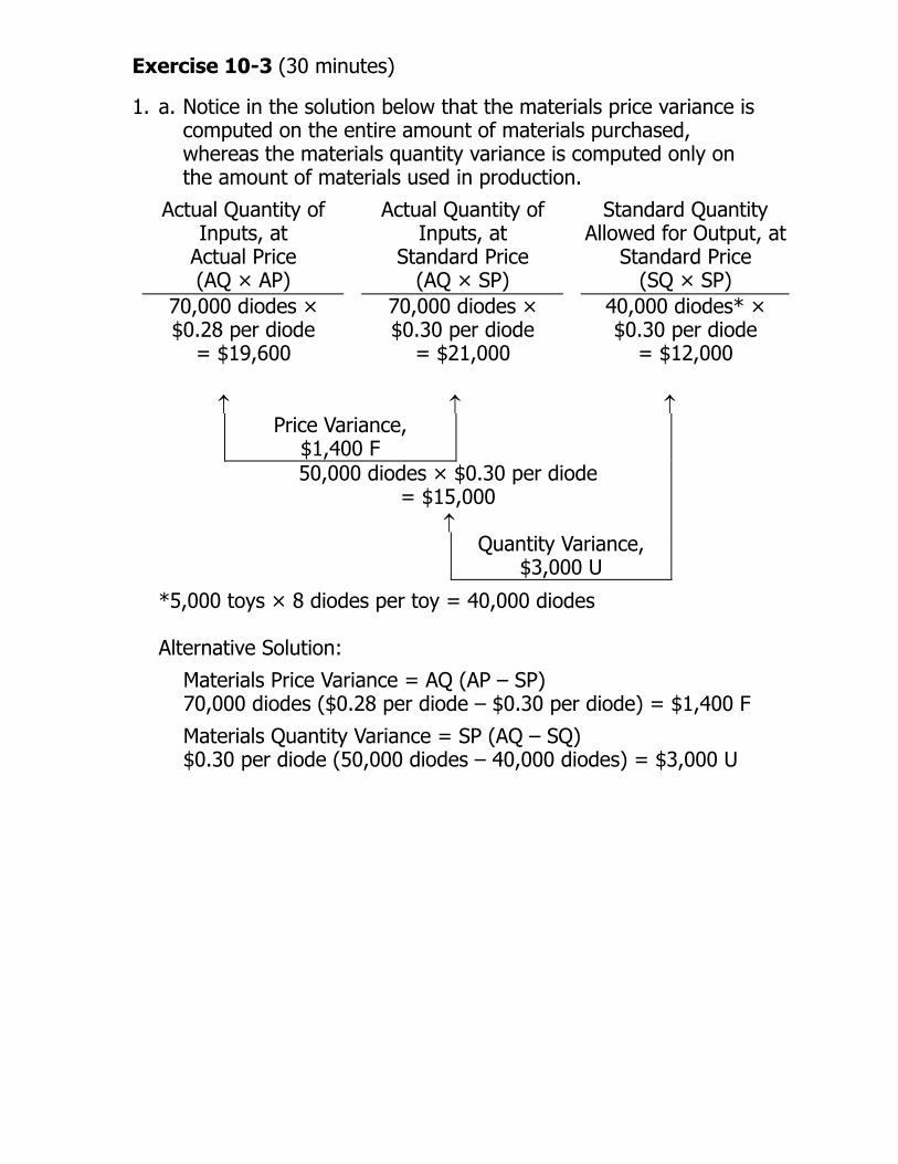
Exercise 10-3 (30 minutes)
1. a. Notice in the solution below that the materials price variance is computed on the entire amount of materials purchased, whereas the materials quantity variance is computed only on the amount of materials used in production.
Actual Quantity of Inputs, at
Actual Price
Actual Quantity of Inputs, at
Standard Price
Standard Quantity Allowed for Output, at
Standard Price (AQ × AP) (AQ × SP)
70,000 diodes × $0.28 per diode
(SQ × SP) 70,000 diodes ×
$0.30 per diode 40,000 diodes* ×
$0.30 per diode = $19,600 = $21,000 = $12,000
↑
↑ ↑Price Variance,
$1,400 F
50,000 diodes × $0.30 per diode = $15,000
↑ Quantity Variance,
$3,000 U
$0.30 per diode (50,000 diodes – 40,000 diodes) = $3,000 U
*5,000 toys × 8 diodes per toy = 40,000 diodes Alternative Solution:
Materials Price Variance = AQ (AP – SP) 70,000 diodes ($0.28 per diode – $0.30 per diode) = $1,400 F
Materials Quantity Variance = SP (AQ – SQ)

Exercise 10-3 (continued)
Actual Hours of Input, at the Actual
Rate
$48,000
b. Direct labor variances:
Actual Hours of Input, at the
Standard Rate
Standard Hours Allowed for Output, at the Standard Rate
(AH × AR) (AH × SR) (SH × SR) 6,400 hours ×
$7 per hour 6,000 hours* ×
$7 per hour = $44,800
↑
= $42,000
↑ ↑Rate Variance,
$3,200 U Efficiency Variance,
$2,800 U
Total Variance, $6,000 U
*5,000 toys × 1.2 hours per toy = 6,000 hours Alternative Solution:
Labor Efficiency Variance = SR (AH – SH) $7 per hour (6,400 hours – 6,000 hours) = $2,800 U
Labor Rate Variance = AH (AR – SR) 6,400 hours ($7.50* per hour – $7.00 per hour) = $3,200 U *$48,000 ÷ 6,400 hours = $7.50 per hour

Exercise 10-3 (continued)
2. A variance usually has many possible explanations. In particular, we should always keep in mind that the standards themselves may be incorrect. Some of the other possible explanations for the variances observed at Topper Toys appear below:
Materials Price VarianceSince this variance is favorable, the actual price paid per unit for the material was less than the standard price. This could occur for a variety of reasons including the purchase of a lower grade material at a discount, buying in an unusually large quantity to take advantage of quantity discounts, a change in the market price of the material, and particularly sharp bargaining by the purchasing department.
Labor Efficiency VarianceSince this variance is unfavorable, the actual number of labor hours was greater than the standard labor hours allowed for the actual output. As with the other variances, this variance could have been caused by any of a number of factors. Some of the possible explanations include poor supervision, poorly trained workers, low quality materials requiring more labor time to process, and machine breakdowns. In addition, if the direct labor force is essentially fixed, an unfavorable labor efficiency variance could be caused by a reduction in output due to decreased demand for the company’s products.
Materials Quantity VarianceSince this variance is unfavorable, more materials were used to produce the actual output than were called for by the standard. This could also occur for a variety of reasons. Some of the possibilities include poorly trained or supervised workers, improperly adjusted machines, and defective materials.
Labor Rate VarianceSince this variance is unfavorable, the actual average wage rate was higher than the standard wage rate. Some of the possible explanations include an increase in wages that has not been reflected in the standards, unanticipated overtime, and a shift toward more highly paid workers.

Exercise 10-8 (20 minutes)
1. Throughput time = Process time + Inspection time + Move time + Queue time
= 2.8 days + 0.5 days + 0.7 days + 4.0 days = 8.0 days
2. Only process time is value-added time; therefore the
manufacturing cycle efficiency (MCE) is:
Value-added time 2.8 days
MCE= = =0.35Throughput time 8.0 days
3. If the MCE is 35%, then the complement of this figure, or 65% of
the time, was spent in non-value-added activities.
= Wait time + Throughput time =
24.0 days
4. Delivery cycle time 16.0 days + 8.0 days = 5. If all queue time in production is eliminated, then the throughput
time drops to only 4 days (0.5 + 2.8 + 0.7). The MCE becomes:
Value-added time 2.8 daysMCE= = =0.70
Throughput time 4.0 days
Thus, the MCE increases to 70%. This exercise shows quite dramatically how the JIT approach can improve operations and reduce throughput time.

Problem 10-10 (45 minutes)
Actual Quantity of Inputs, at
Standard Price
1. a. In the solution below, the materials price variance is computed on the entire amount of materials purchased, whereas the materials quantity variance is computed only on the amount of materials used in production:
Actual Quantity of Inputs, at
Actual Price
Standard Quantity Allowed for Output, at Standard Price
(AQ × AP) (AQ × SP) 4,500 pounds* ×
$6.00 per pound
(SQ × SP) $46,000 8,000 pounds ×
$6.00 per pound
↑
= $48,000 = $27,000
↑ ↑
Price Variance, $2,000 F 6,000 pounds × $6.00 per pound
= $36,000 ↑
Quantity Variance, $9,000 U
*3,000 units × 1.5 pounds per unit = 4,500 pounds Alternatively:
Materials Quantity Variance = SP (AQ – SQ)
Materials Price Variance = AQ (AP – SP) 8,000 pounds ($5.75 per pound* – $6.00 per pound) = $2,000
F *$46,000 ÷ 8,000 pounds = $5.75 per pound
$6 per pound (6,000 pounds – 4,500 pounds) = $9,000 U
Problem 10-10 (continued)
b. No, the contract should probably not be signed. Although the new supplier is offering the materials at only $5.75 per pound, the materials do not seem to hold up well in production as shown by the large materials quantity variance. Moreover, the company still has 2,000 pounds of the material in the warehouse unused; if these materials do as poorly in production as the 6,000 pounds already used, the total quantity variance on the 8,000 pounds of materials purchased will be very large indeed.

Problem 10-10 (continued)
1,600 hours × $12.00 per hour
1,800 hours** × $12.00 per hour
2. a. Actual Hours of Input, at the Actual Rate
Actual Hours of Input, at the
Standard Rate
Standard Hours Allowed for Output, at the Standard Rate
(AH × AR) (AH × SR) (SH × SR) 1,600 hours* × $12.50 per hour
= $20,000 = $19,200 = $21,600
↑ ↑Rate Variance,
$800 U Efficiency Variance,
$2,400 F
↑
Total Variance, $1,600 F
* 10 workers × 160 hours per worker = 1,600 hours ** = 1,800 hours
$12.00 per hour (1,600 hours – 1,800 hours) = $2,400 F
b. Yes, the new labor mix should probably be continued. Although it increases the average hourly labor cost from $12.00 to $12.50, thereby causing an $800 unfavorable labor rate variance, this is more than offset by greater efficiency of labor time. Notice that the labor efficiency variance is $2,400 favorable. Thus, the new labor mix reduces overall labor costs.
3,000 units × 0.6 hours per unit
Alternatively:
Labor Rate Variance = AH (AR – SR) 1,600 hours ($12.50 per hour – $12.00 per hour) = $800 U
Labor Efficiency Variance = SR (AH – SH)

Problem 10-10 (continued)
3.
(AH × AR) $3,600 1,600 hours ×
$2.50 per hour
Actual Hours of Input, at the Actual Rate
Actual Hours of Input, at the
Standard Rate
Standard Hours Allowed for Output, at the Standard Rate
(AH × SR) (SH × SR) 1,800 hours ×
$2.50 per hour = $4,000 = $4,500
↑ ↑ ↑Spending Variance,
$400 F Efficiency Variance,
$500 F
Total Variance, $900 F
Alternatively:
1,600 hours ($2.25 per hour* – $2.50 per hour) = $400 F
$2.50 per hour (1,600 hours – 1,800 hours) = $500 F
Both the labor efficiency variance and the variable overhead efficiency variance are computed by comparing actual labor-hours to standard labor-hours. Thus, if the labor efficiency variance is favorable, then the variable overhead efficiency variance will be favorable as well.
Variable Overhead Spending Variance = AH (AR – SR)
*$3,600 ÷ 1,600 hours = $2.25 per hour
Variable Overhead Efficiency Variance = SR (AH – SH)

Problem 10-11 (45 minutes)
1. The standard quantity of plates allowed for tests performed during the month would be:
Smears ................................... 2,700Blood tests .............................. 900Total ....................................... 3,600Plates per test ......................... 3 ×Standard quantity allowed ........ 10,800
The variance analysis for plates would be:
Actual Quantity of Inputs, at
Actual Price
$38,400
Actual Quantity of Inputs, at
Standard Price
Standard Quantity Allowed for Output, at Standard Price
(AQ × AP) (AQ × SP) (SQ × SP) 16,000 plates × $2.50 per plate
10,800 plates × $2.50 per plate
= $40,000 = $27,000
↑ ↑ ↑
$1,600 F
Price Variance,
14,000 plates × $2.50 per plate = $35,000
↑ Quantity Variance,
$8,000 U Alternative Solution:
Materials Price Variance = AQ (AP – SP)
16,000 plates ($2.40 per plate* – $2.50 per plate) = $1,600 F *$38,400 ÷ 16,000 plates = $2.40 per plate.
Materials Quantity Variance = SP (AQ – SQ) $2.50 per plate (14,000 plates – 10,800 plates) = $8,000 U

Problem 10-11 (continued)
Note that all of the price variance is due to the hospital’s 4% quantity discount. Also note that the $8,000 quantity variance for the month is equal to nearly 30% of the standard cost allowed for plates. This variance may be the result of using too many assistants in the lab.
2. a. The standard hours allowed for tests performed during the month would be:
Smears: 0.3 hour per test × 2,700 tests ...... 810
Blood tests: 0.6 hour per test × 900 tests.... 540 Total standard hours allowed ...................... 1,350
The variance analysis of labor would be:
Actual Hours of Input, at the Actual Rate
Standard Hours Allowed for Output, at the Standard Rate
(AH × SR) $18,450 1,800 hours ×
$12 per hour 1,350 hours ×
$12 per hour
Actual Hours of Input, at the
Standard Rate
(AH × AR) (SH × SR)
= $16,200
↑ ↑
= $21,600
↑Rate Variance,
$3,150 F Efficiency Variance,
$5,400 U
Total Variance, $2,250 U
Labor Rate Variance = AH (AR – SR)
*$18,450 ÷ 1,800 hours = $10.25 per hour
Labor Efficiency Variance = SR (AH – SH)
Alternative Solution:
1,800 hours ($10.25 per hour* – $12.00 per hour) = $3,150 F
$12 per hour (1,800 hours – 1,350 hours) = $5,400 U
Problem 10-11 (continued)
b. The policy probably should not be continued. Although the hospital is saving $1.75 per hour by employing more assistants relative to the number of senior technicians than other hospitals, this savings is more than offset by other factors. Too much time is being taken in performing lab tests, as indicated by the large unfavorable labor efficiency variance. And, it seems likely that most (or all) of the hospital’s unfavorable quantity variance for plates is traceable to inadequate supervision of assistants in the lab.
3. The variable overhead variances follow:
Actual Hours of Input, at the
Standard Rate
Standard Hours Allowed for Output, at the Standard Rate
(AH × AR) (SH × SR)
Actual Hours of Input, at the Actual Rate
(AH × SR) $11,700 1,800 hours ×
$6 per hour 1,350 hours ×
$6 per hour = $10,800 = $8,100
↑ ↑ ↑Efficiency Variance,
$2,700 U
Spending Variance, $900 U
Total Variance, $3,600 U
Alternative Solution:
*$11,700 ÷ 1,800 hours = $6.50 per hour
Variable Overhead Spending Variance = AH (AR – SR) 1,800 hours ($6.50 per hour* – $6.00 per hour) = $900 U
Variable Overhead Efficiency Variance = SR (AH – SH) $6 per hour (1,800 hours – 1,350 hours) = $2,700 U Yes, the two variances are related. Both are computed by
comparing actual labor time to the standard hours allowed for the output of the period. Thus, if there is an unfavorable labor efficiency variance, there will also be an unfavorable variable overhead efficiency variance.

Problem 10-13 (45 minutes)
1. a. Actual Quantity of
Inputs, at Actual Price
Actual Quantity of Inputs, at
Standard Price
Standard Quantity Allowed for Output, at Standard Price
(AQ × AP) 25,000 pounds × $2.95 per pound
20,000 pounds* × $2.50 per pound
(AQ × SP) (SQ × SP) 25,000 pounds × $2.50 per pound
= $73,750 = $62,500 = $50,000
↑ ↑
↑
Price Variance, $11,250 U 19,800 pounds × $2.50 per pound
= $49,500 ↑
Quantity Variance, $500 F
*5,000 ingots × 4.0 pounds per ingot = 20,000 pounds Alternatively:
Materials Quantity Variance = SP (AQ – SQ) $2.50 per pound (19,800 pounds – 20,000 pounds) = $500 F
Materials Price Variance = AQ (AP – SP) 25,000 pounds ($2.95 per pound – $2.50 per pound) = $11,250
U

Problem 10-13 (continued)
Actual Hours of Input, at the
Standard Rate
(AH × SR) (SH × SR) 3,600 hours ×
$9.00 per hour
b. Actual Hours of Input, at the Actual Rate
Standard Hours Allowed for Output, at the Standard Rate
(AH × AR) 3,600 hours × $8.70 per hour
3,000 hours* × $9.00 per hour
= $31,320 = $27,000
↑
= $32,400
↑ ↑Rate Variance,
$1,080 F Efficiency Variance,
$5,400 U
Total Variance, $4,320 U
*5,000 ingots × 0.6 hour per ingot = 3,000 hours Alternatively:
$9.00 per hour (3,600 hours – 3,000 hours) = $5,400 U
Labor Rate Variance = AH (AR – SR) 3,600 hours ($8.70 per hour – $9.00 per hour) = $1,080 F
Labor Efficiency Variance = SR (AH – SH)

Problem 10-13 (continued)
Standard Hours Allowed for Output, at the Standard Rate
(AH × AR) (AH × SR) (SH × SR) 1,800 hours × $2.00 per hour
c. Actual Hours of Input, at the Actual Rate
Actual Hours of Input, at the
Standard Rate
$4,320 1,500 hours* ×
$2.00 per hour = $3,600 = $3,000
↑ ↑
↑Spending Variance,
$720 U Efficiency Variance,
$600 U
Total Variance, $1,320 U
*5,000 ingots × 0.3 hours per ingot = 1,500 hours
1,800 hours ($2.40 per hour* – $2.00 per hour) = $720 U *$4,320 ÷ 1,800 hours = $2.40 per hour
Alternatively:
Variable Overhead Spending Variance = AH (AR – SR)
Variable Overhead Efficiency Variance = SR (AH – SH) $2.00 per hour (1,800 hours – 1,500 hours) = $600 U

Problem 10-13 (continued)
U Material quantity variance ........................ F Labor rate variance.................................. 1,080 F
5,400 U
2. Summary of variances:
Material price variance ............................. $11,250 500
Labor efficiency variance..........................Variable overhead spending variance......... 720 U Variable overhead efficiency variance ........ 600 U Net variance............................................ $16,390 U
The net unfavorable variance of $16,390 for the month caused the plant’s variable cost of goods sold to increase from the budgeted level of $80,000 to $96,390:
Budgeted cost of goods sold at $16 per ingot ........
$80,000Add the net unfavorable variance (as above) ......... 16,390Actual cost of goods sold ..................................... $96,390
This $16,390 net unfavorable variance also accounts for the difference between the budgeted net operating income and the actual net loss for the month.
Budgeted net operating income............................
. $15,000Deduct the net unfavorable variance added to
cost of goods sold for the month ........................ 16,390Net operating loss ................................................ $(1,390)
Materials Price Variance: Outdated standards, uneconomical quantity purchased, higher quality materials, high-cost method of transport.
Poorly trained workers, poor quality materials, faulty equipment, work interruptions, inaccurate standards, insufficient demand.
3. The two most significant variances are the materials price variance
and the labor efficiency variance. Possible causes of the variances include:
Labor Efficiency Variance:

Exercise 11-4 (15 minutes)
Swan Company Flexible Budget
Cost
Formula Machine-Hours
Overhead Costs per MH 8,000 Variable:
9,000 10,000
Supplies................................ $0.20 1,600 $ 1,800 $ 2,000 $Indirect labor ........................ 0.25 2,000 2,250 2,500Utilities ................................. 0.15 1,200 1,350 1,500Maintenance ......................... 0.10 800 900 1,000
Total variable overhead cost...... $0.70 5,600 6,300 7,000
Fixed: Indirect labor ........................ 10,000 10,000 10,000Maintenance ......................... 7,000 7,000 7,000Depreciation.......................... 8,000 8,000 8,000
Total fixed overhead cost .......... 25,000 25,000 25,000
Total overhead cost .................. $30,600 $31,300 $32,000
Exercise 11-5 (20 minutes)
1. Whaley Company Variable Manufacturing Overhead Performance Report
$ 800
F 3,300
Rework time ..........................
Budgeted machine-hours............. 18,000 Actual machine-hours worked ...... 16,000
Actual 16,000 hours
Budget 16,000 hours
Spending Variance
Variable overhead costs: Utilities.................................. $20,000 $19,200 U Supplies ................................ 4,700 4,800 100 Maintenance .......................... 35,100 38,400 F
12,300 9,600 2,700 U Total variable overhead cost.... $72,100 $ 100 U $72,000
2. Favorable variances can be as much a matter of managerial
concern as unfavorable variances. In this case, the favorable maintenance variance undoubtedly would require investigation. Efforts should be made to determine if maintenance is not being carried out. In terms of percentage deviation from budgeted allowances, the rework time variance is even more significant (equal to 28% of the budget allowance). It may be that this unfavorable variance in rework time is a result of poor maintenance of machines. Some may say that if the two variances are related, then the trade-off is a good one, since the savings in maintenance cost is greater than the added cost of rework time. But this is shortsighted reasoning. Poor maintenance can reduce the life of equipment, as well as decrease overall output. These long-run costs may swamp any short-run savings.
Exercise 11-7 (20 minutes)
1. $33,200Overall rate: =$4.15 per MH
8,000 MHs
$8,400Variable rate: =$1.05 per MH
8,000 MHs
$24,800Fixed rate: =$3.10 per MH
8,000 MHs

2. The standard hours per unit of product are: 8,000 MHs ÷ 3,200 units = 2.5 MHs per unit
The standard hours allowed for the actual production would be: 3,500 units × 2.5 MHs per unit = 8,750 MHs 3. Variable overhead
spending variance = (AH × AR) – (AH × SR)
= $935 U
= ($9,860) – (8,500 MHs × $1.05 per MH) = ($9,860) – ($8,925)
Variable overhead efficiency variance = SR (AH – SH)
= $1.05 per MH (8,500 MHs – 8,750 MHs) = $262.50 F

Exercise 11-7 (continued)
Fixed overhead budget and volume variances:
Fixed Overhead Cost Applied to
Work in Process
Actual Fixed
Overhead Cost
Budgeted Fixed Overhead Cost
$25,100 $24,800* 8,750 standard MHs
$300 U
× $3.10 per MH = $27,125
↑ ↑ ↑ Budget Variance, Volume Variance,
$2,325 F
Total Variance, $2,025 F
*8,000 denominator MHs × $3.10 per MH = $24,800. Alternative approach to the budget variance:
Budget Actual Fixed Budgeted Fixed= - Variance Overhead Cost Overhead Cost
= $25,100 - $24,800 = $300 U
Alternative approach to the volume variance:
( )Fixed Portion ofVolume Denominator Standard Hours=the Predetermined - Variance Hours AllowedOverhead Rate
= $3.10 per MH (8,000 MHs - 8,750 MHs) = $2,325 F
Problem 11-12 (30 minutes)
r
Variable overhead costs: U
5,400
1. The reports as presently prepared are of little use to the company. The problem is that the company is using a static budget approach, and is comparing budgeted performance at one level of activity to actual performance at another level of activity. Although the reports do a good job of showing whether or not the budgeted level of activity was attained, they do not tell whether costs were controlled for the period.
2. The company should use a flexible budget approach to evaluate
control over costs. Under the flexible budget approach, the actual costs incurred during the quarter in working 25,000 hours should be compared to budgeted costs at that activity level.
3. Shipley Company Overhead Performance Report—Milling Department For the Quarter Ended June 30
Budgeted machine-hours.......... 30,000 MHs Actual machine-hours............... 25,000 MHs
Overhead Costs
Cost Fo mula (per MH)
Actual 25,000 hours
Budget 25,000 hours
Spending or Budget Variance
Indirect labor ............... $0.75 20,000 $ 18,750 $ $1,250Supplies....................... 0.20 5,000 400 UUtilities ........................ 1.00 27,000 25,000 2,000 URework time................. 0.50 14,000 12,500 1,500 U
Total variable costs.......... $2.45 66,400 61,250 5,150 U
Maintenance ................Inspection....................
Fixed overhead costs: 61,900 60,000 1,900 U
90,000 90,000 — Total fixed costs.............. 151,900 150,000 1,900 U
Total overhead costs........ $218,300 $211,250 $7,050 U

Problem 11-13 (30 minutes)
1. Direct materials, 4 pounds at $2.60 per pound........................18.00
$10.40 Direct labor, 2 DLHs at $9.00 per DLH .................................... Variable manufacturing overhead, 2 DLHs at $3.80 per DLH* ... 7.60 Fixed manufacturing overhead, 2 DLHs at $7.00 per DLH** ..... 14.00 Standard cost per unit........................................................... $50.00
* $34,200 ÷ 9,000 DLHs = $3.80 per DLH
2. Materials variances:
Materials Price Variance = AQ (AP – SP)
** $63,000 ÷ 9,000 DLHs = $7.00 per DLH
30,000 pounds ($2.50 per pound – $2.60 per pound) = $3,000 F
Materials Quantity Variance = SP (AQ – SQ) $2.60 per pound (20,000 pounds – 19,200 pounds*) = $2,080
U *4,800 units × 4 pounds per unit = 19,200 pounds Labor variances:
Labor Rate Variance = AH (AR – SR) 10,000 DLHs ($8.60 per DLH – $9.00 per DLH) = $4,000 F
Labor Efficiency Variance = SR (AH – SH) $9 per DLH (10,000 DLHs – 9,600 DLHs*) = $3,600 U *4,800 units × 2 DLHs per unit = 9,600 DLHs

Problem 11-13 (continued)
3. Variable manufacturing overhead variances:
Actual Hours of Input, at the Actual
Rate
Actual Hours of Input, at the
Standard Rate
Standard Hours Allowed for Output, at the Standard Rate
(AH × AR) (AH × SR) (SH × SR) $35,900 10,000 DLHs ×
$3.80 per DLH 9,600 DLHs ×
$3.80 per DLH = $38,000 = $36,480
↑ ↑
$2,100 F Efficiency Variance,
↑ Spending Variance,
$1,520 U
Total Variance, $580 F
Alternative solution for the variable overhead variances:
Variable Overhead Spending Variance = (AH × AR) – (AH × SR) ($35,900) – (10,000 DLHs × $3.80 per DLH) = $2,100 F
Variable Overhead Efficiency Variance = SR (AH – SH)
Budgeted Fixed Overhead Cost
$3.80 per DLH (10,000 DLHs – 9,600 DLHs) = $1,520 U Fixed manufacturing overhead variances:
Actual Fixed
Overhead Cost
Fixed Overhead Cost Applied to
Work in Process $64,800 $63,000 9,600 DLHs ×
$7 per DLH
= $67,200
↑ ↑ ↑
$4,200 F Budget Variance,
$1,800 U Volume Variance,

Problem 11-13 (continued)
Alternative approach to the budget variance:
Budget Actual Fixed Budgeted Fixed= - Variance Overhead Cost Overhead Cost
=$64,800 – $63,000 = $1,800 U Alternative approach to the volume variance:
( )Fixed Portion ofVolume Denominator Standard Hours=the Predetermined - Variance Hours AllowedOverhead Rate
=$7 per DLH (9,000 DLHs – 9,600 DLHs) = $4,200 F 4. The choice of a denominator activity level affects standard unit
costs in that the higher the denominator activity level chosen, the lower standard unit costs will be. The reason is that the fixed portion of overhead costs is spread more thinly as the denominator activity figure rises.
The volume variance cannot be controlled by controlling spending. Rather, the volume variance simply reflects whether actual activity was greater or less than the denominator activity. Thus, the volume variance is controllable only through activity.
Exercise 13-4 (30 minutes)
1.
Per Unit Diffe ential
Costsr
15,000 units Make Buy
Direct materials ........................... 90,000 $ 120,000
30,000 Fixed manufacturing overhead,
common...................................
Make Buy Cost of purchasing ....................... $20 $300,000 6 $
Direct labor ................................. 8 Variable manufacturing overhead .. 1 15,000
Fixed manufacturing overhead, traceable1 ................................. 2
0 0 0 0 Total costs................................... $17 $20 $255,000 $300,000
Difference in favor of continuing
to make the parts...................... $3 $45,000
Cost of purchasing (part 1)............................
Opportunity cost—segment margin forgone on a potential new product line ...................
1 Only the supervisory salaries can be avoided if the parts are purchased. The remaining book value of the special equipment is a sunk cost; hence, the $3 per unit depreciation expense is not relevant to this decision. Based on these data, the company should reject the offer and should continue to produce the parts internally.
2. Make Buy
$300,000 Cost of making (part 1) ................................. $255,000
65,000 Total cost ..................................................... $320,000 $300,000
Difference in favor of purchasing from the
outside supplier.......................................... $20,000
Thus, the company should accept the offer and purchase the parts from the outside supplier.

Exercise 13-5 (15 minutes)
Only the incremental costs and benefits are relevant. In particular, only the variable manufacturing overhead and the cost of the special tool are relevant overhead costs in this situation. The other manufacturing overhead costs are fixed and are not affected by the decision.
Per TotalUnit 10 bracelets
Incremental revenue................................ $349.95 $3,499.50 Incremental costs:
70.00 Special filigree....................................
Variable costs: Direct materials .................................. 143.00 1,430.00 Direct labor ........................................ 86.00 860.00 Variable manufacturing overhead......... 7.00 6.00 60.00 Total variable cost................................. $242.00 2,420.00 Fixed costs:
Purchase of special tool....................... 465.00 Total incremental cost.............................. 2,885.00 Incremental net operating income............. $ 614.50
Even though the price for the special order is below the company's regular price for such an item, the special order would add to the company's net operating income and should be accepted. This conclusion would not necessarily follow if the special order affected the regular selling price of bracelets or if it required the use of a constrained resource.

Exercise 13-6 (30 minutes)
1. (1) $18
8
2.0Contribution margin per direct labor-hour (1) ÷ (4)... $10
2. The company should concentrate its labor time on producing product
A:
Direct labor-hours available .......................
A B C Contribution margin per unit ................................... $36 $20
(2) Direct labor cost per unit......................................... $12 $32 $16 (3) Direct labor rate per hour........................................ 8 8 (4) Direct labor-hours required per unit (2) ÷ (3) ........... 1.5 4.0 $12 9 $
A B CContribution margin per direct labor-hour ... $12 $9 $10
× 3,000 × 3,000 × 3,000Total contribution margin........................... $36,000 $27,000 $30,000
Although product A has the lowest contribution margin per unit and the second lowest contribution margin ratio, it has the highest contribution margin per direct labor-hour. Since labor time seems to be the company’s constraint, this measure should guide management in its production decisions.
3. The amount Banner Company should be willing to pay in overtime
wages for additional direct labor time depends on how the time would be used. If there are unfilled orders for all of the products, Banner would presumably use the additional time to make more of product A. Each hour of direct labor time generates $12 of contribution margin over and above the usual direct labor cost. Therefore, Banner should be willing to pay up to $20 per hour (the $8 usual wage plus the contribution margin per hour of $12) for additional labor time, but would of course prefer to pay far less. The upper limit of $20 per direct labor hour signals to managers how valuable additional labor hours are to the company.

Exercise 13-6 (continued)
If all the demand for product A has been satisfied, Banner Company would then use any additional direct labor-hours to manufacture product C. In that case, the company should be willing to pay up to $18 per hour (the $8 usual wage plus the $10 contribution margin per hour for product C) to manufacture more product C.
Likewise, if all the demand for both products A and C has been satisfied, additional labor hours would be used to make product B. In that case, the company should be willing to pay up to $17 per hour to manufacture more product B.

Exercise 13-8 (30 minutes)
1. The relevant costs of a fishing trip would be:
Fuel and upkeep on boat per trip ....... $25Junk food consumed during trip* ....... 8Snagged fishing lures........................ 7Total ................................................ $40
* The junk food consumed during the trip may not be completely relevant. Even if Steve were not going on the trip, he would still have to eat. The amount by which the cost of the junk food exceeds the cost of the food he would otherwise consume would be the relevant amount.
The other costs are sunk at the point at which the decision is made to go on another fishing trip.
2. If he fishes for the same amount of time as he did on his last trip,
all of his costs are likely to be about the same as they were on his last trip. Therefore, it really doesn’t cost him anything to catch the last fish. The costs are really incurred in order to be able to catch fish and would be the same whether one, two, three, or a dozen fish were actually caught. Fishing, not catching fish, costs money. All of the costs are basically fixed with respect to how many fish are actually caught during any one fishing trip, except possibly the cost of snagged lures.
3. In a decision of whether to give up fishing altogether, nearly all of
the costs listed by Steve’s wife are relevant. If he did not fish, he would not need to pay for boat moorage, new fishing gear, a fishing license, fuel and upkeep, junk food, or snagged lures. In addition, he would be able to sell his boat, the proceeds of which would be considered relevant in this decision. The original cost of the boat, which is a sunk cost, would not be relevant.

Exercise 13-8 (continued)
These three requirements illustrate the slippery nature of costs. A cost that is relevant in one situation can be irrelevant in the next. None of the costs are relevant when we compute the cost of catching a particular fish; some of them are relevant when we compute the cost of a fishing trip; and nearly all of them are relevant when we consider the cost of not giving up fishing. What is even more confusing is that Wendy is correct; the average cost of a salmon is $167, even though the cost of actually catching any one fish is essentially zero. It may not make sense from an economic standpoint to have salmon fishing as a hobby, but as long as Steve is out in the boat fishing, he might as well catch as many fish as he can.

Problem 13-18 (60 minutes)
1. The $2.00 per unit general overhead cost is not relevant to the decision, since the total general company overhead cost will be the same regardless of whether the company decides to make or buy the subassemblies. Also, the depreciation on the old equipment is not a relevant cost since it represents a sunk cost and the old equipment is worn out and must be replaced. The cost of supervision is relevant since this cost can be avoided by buying the subassemblies.
r
Total Differential Costs for
40,000 Units Make
18,000
Equipment rental* .................
Diffe ential
Costs Per Unit Make Buy Buy Outside supplier’s price .......... $8.00 $320,000 Direct materials ..................... $2.75 $110,000 Direct labor ($4.00 × 0.75)..... 3.00 120,000 Variable overhead
($0.60 × 0.75) ................... 0.45 Supervision ........................... 0.75 30,000
1.50 60,000 Total ..................................... $8.45 $8.00 $338,000 $320,000
Difference in favor of buying... $0.45 $18,000
* $60,000 per year ÷ 40,000 units per year = $1.50 per unit

Problem 13-18 (continued)
2. a. Notice that unit costs for both supervision and equipment rental will change if the company needs 50,000 subassemblies each year. These fixed costs will be spread over a larger number of units, thereby decreasing the cost per unit.
r f
Diffe ential Costs Per Unit
Total Dif erential Costs—50,000 Units
Make Buy
$2.75150,000 22,500
Supervision
Make Buy Outside supplier’s price ............ $8.00 $400,000 Direct materials ....................... $137,500 Direct labor ............................. 3.00 Variable overhead .................... 0.45
($30,000 ÷ 50,000 units)....... 0.60 30,000
Equipment rental ($60,000 ÷ 50,000 units)....... 1.20 60,000
Total ....................................... $8.00 $8.00 $400,000 $400,000
Difference ............................... $0 $0
The company would be indifferent between the two alternatives if 50,000 subassemblies were needed each year.

Problem 13-18 (continued)
b. Again, notice that the unit costs for both supervision and equipment rental decrease with the greater volume of units.
Differential Costs Per
Unit f
Total Dif erential
Costs—60,000 Units Make Buy
Direct materials ....................... $2.75
Variable overhead....................
1.00
Make Buy Outside supplier’s price ............ $8.00 $480,000 $165,000 Direct labor ............................. 3.00 180,000
0.45 27,000 Supervision
($30,000 ÷ 60,000 units) ...... 0.50 30,000 Equipment rental
($60,000 ÷ 60,000 units) ...... 60,000 Total....................................... $7.70 $8.00 $462,000 $480,000
Difference in favor of making.... $0.30 $18,000
The company should purchase the new equipment and make the subassemblies if 60,000 units per year are needed.

Problem 13-18 (continued)
3. Other factors that the company should consider include:
a. Will volume in future years be increasing, or will it remain constant at 40,000 units per year? (If volume increases, then buying the new equipment becomes more desirable, as shown in the computations above.)
f. If the outside supplier’s offer is accepted and the need for subassemblies increases in future years, will the supplier have the capacity to provide more than 40,000 subassemblies per year?
b. Can quality control be maintained if the subassemblies are purchased from the outside supplier?
c. Does the company have some other profitable use for the space now being used to produce the subassemblies? Does production of the subassemblies require use of a constrained resource?
d. Will the outside supplier be dependable in meeting shipping schedules?
e. Can the company begin making the subassemblies again if the supplier proves to be undependable, or are there alternative suppliers?

Problem 13-19 (45 minutes)
1. Selling price per unit ........................ $40 Less variable expenses per unit*....... 24 Contribution margin per unit............. $16
*$9.50 + $10.00 + $2.80 + $1.70 = $24.00
Increased unit sales (80,000 × 25%) ..................... 20,000Contribution margin per unit .................................. × $16Incremental contribution margin ............................ $320,000Less added fixed selling expense............................ 150,000Incremental net operating income.......................... $170,000
Yes, the increase in fixed selling expense would be justified. 2. Variable production cost per unit............................ $22.30 Import duties, etc. ($14,000 ÷ 20,000 units) .......... 0.70 Shipping cost per unit ........................................... 1.50 Break-even price per unit ...................................... $24.50
Fixed manufacturing overhead cost ($400,000 × 3/12 = $100,000; $100,000 × 40%) ....................................
3. If the plant operates at 25% of normal levels, then only 5,000 units will be produced and sold during the three-month period:
80,000 units per year × 3/12 = 20,000 units. 20,000 units × 25% = 5,000 units produced and sold.
Given this information, the simplest approach to the solution is:
Contribution margin lost if the plant is closed (5,000 units × $16 per unit*) .......................... $(80,000)
Fixed costs that can be avoided if the plant is closed:
$40,000 Fixed selling cost ($360,000 × 3/12 =
$90,000; $90,000 × 1/3) ........................... 30,000 70,000Net disadvantage of closing the plant ................. $(10,000)
*$40.00 – ($9.50 + $10.00 + $2.80 + $1.70) = $16.00

Problem 13-19 (continued)
Alternative approach:
Close the Plant
$ 200,000 $ 0
Keep the Plant Open
Sales (5,000 units × $40 per unit).................Less variable expenses
(5,000 units × $24 per unit)....................... 120,000 0 Contribution margin ..................................... 80,000 0 Less fixed expenses:
Fixed manufacturing overhead cost: $400,000 × 3/12 ....................................$400,000 × 3/12 × 60% .........................
90,000 $360,000 × 3/12 × 2/3 ...........................
100,000
60,000 Fixed selling expense:
$360,000 × 3/12 .................................... 60,000
Total fixed expenses..................................... 190,000 120,000 Net operating income (loss) .......................... $(110,000) $(120,000)
5. The costs that can be avoided by purchasing from the outside supplier are relevant. These costs are:
Variable production costs................................................
4. The relevant cost is $1.70 per unit, which is the variable selling expense per Zet. Since the blemished units have already been produced, all production costs (including the variable production costs) are sunk. The fixed selling expenses are not relevant since they will remain the same regardless of whether or not the blemished units are sold. The variable selling expense may or may not be relevant—depending on how the blemished units are sold. For example, the units may be sold through a liquidator without incurring the normal variable selling expense.
$22.30Fixed manufacturing overhead cost ($400,000 × 70% =
$280,000; $280,000 ÷ 80,000 units)............................. 3.50Variable selling expense ($1.70 × 60%)........................... 1.02Total avoidable cost........................................................ $26.82
To be acceptable, the outside manufacturer’s quotation must be less than $26.82 per unit.

Exercise 14-13 (30 minutes)
1. Investment in the projectFactor of the internal = rate of return Annual cash inflow
$136,700= = 5.468
$25,000
Looking in Table 14C-4 and scanning along the 14-period line, a
factor of 5.468 represents an internal rate of return of 16%.
Item Year(s)16%
Factor Initial investment.... Now 1.000
2. Amount of Cash Flows
Present Value of Cash Flows
$(136,700) $(136,700)
Net annual cash
inflows ................ 1-14 25,000 5.468 136,700 Net present value ... $ 0
The reason for the zero net present value is that 16% (the discount rate we have used) represents the machine’s internal rate of return. The internal rate of return is the rate that causes the present value of a project’s cash inflows to just equal the present value of the investment required.
3.
Investment in the projectFactor of the internal = rate of return Annual cash inflow
$136,700= = 6.835
$20,000
Looking in Table 14C-4 and scanning along the 14-period line, the 6.835 factor is closest to 6.982, the factor for the 11% rate of return. Thus, to the nearest whole percent, the internal rate of return is 11%.

Problem 14-21 (20 minutes)
Items and Computations Year(s)
(2) Tax
Effect -(1)
Amount
(1) × (2) After Tax
Cash Flows1
FInvestment in new trucks.................... Now $(450,000) $(450,000) 1Salvage from sale of the old trucks ...... Now 30,000 1 – 0.30 21,000 1Net annual cash receipts..................... 1-8 108,000 1 – 0.30 75,600 4Depreciation deductions*.................... 1-8 56,250 0.30 16,875 4Overhaul of motors ............................ (45,000) 1 – 0.30 (31,500)5 0Salvage from the new trucks............... 8 20,000 1 – 0.30 14,000 0Net present value...............................
* $450,000 ÷ 8 years = $56,250 per year
Since the project has a positive net present value, the contract should be accepted.
Problem 14-28 (30 minutes)
1. The net present value analysis would be: (2) Tax
Effect -
Items and Computations Year(s)(1)
Amount
(1) × (2) After Tax
Cash Flows10%
FactInvestment in equipment ................ Now $(600,000) $(600,000) 1.0Working capital needed .................. Now (85,000) (85,000) 1.0Net annual cash receipts................. 1-10 1 – 0.30 77,000 6.110,000 1Depreciation deductions ................. 1-10 18,000 6.60,000 0.30 1Cost of restoring land....................... 10 (49,000) 0.(70,000) 1 – 0.30 3Salvage value of the equipment*...... 10 0.90,000 1 – 0.30 63,000 3Working capital released................. 10 85,000 85,000 0.3Net present value...........................
*$600,000 × 15% = $90,000. 2. No, the investment project should not be undertaken. It has a
negative net present value when the company’s cost of capital is used as the discount rate.