1

Exercise 16: Terrain Analysis

Raster analysis has been explored in previous exercises. Here, we will focus specifically on terrain analysis using digital elevation models (DEMs). This exercise describes how to produce a variety of terrain derivatives from DEMs. The processes outlined here make use of a variety of raster analysis tools and techniques. In the last part of the lab, you will produce a cut and fill model by differencing two DEMs.

The DEM that will be used at the beginning of this exercise covers a portion of Preston County, West Virginia. It was derived from light detection and ranging (LiDAR) data at a 5 m spatial resolution. The raw LiDAR data are available here: http://tagis.dep.wv.gov/home/?q=Downloads. They can also be obtained from West Virginia View: http://www.wvgis.wvu.edu/lidar/. A later lab exercise will show how to process raw LiDAR data. It should be noted that these data will support the creation of a 1 m resolution DEM; however, a 5 m DEM will be used in this lab to reduce file size and processing time. For the last part of the lab, two separate DEMs will be used. They were also both generated from LiDAR data. As surface mining occurred between the collections of these datasets, the extent of elevation or terrain change can be assessed by differencing these surfaces.

Topics covered in this exercise include:

1. Create slope, aspect, and hillshade raster grids from a DEM 2. Create and interpret surface curvature grids 3. Use neighborhood analysis and raster math to produce more complex

terrain outputs 4. Difference two DEMs to obtain cut and fill extents

Step 1. Open a Map Project

First, we need to download and open the Exercise_16.aprx file.

� Download the Exercise_16 lab folder from the class webpage under Education tab on http://www.wvview.org/. All lab material is available under “Labs and Data” tab.

� Click on the “L16 Data” button to download the Exercise_16.zip file. � You will need to extract the compressed files and save it to the

location of your choosing.

2

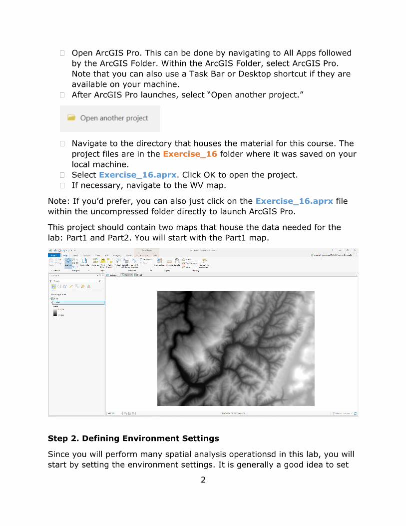
� Open ArcGIS Pro. This can be done by navigating to All Apps followed by the ArcGIS Folder. Within the ArcGIS Folder, select ArcGIS Pro. Note that you can also use a Task Bar or Desktop shortcut if they are available on your machine.

� After ArcGIS Pro launches, select “Open another project.”

� Navigate to the directory that houses the material for this course. The project files are in the Exercise_16 folder where it was saved on your local machine.

� Select Exercise_16.aprx. Click OK to open the project. � If necessary, navigate to the WV map.

Note: If you’d prefer, you can also just click on the Exercise_16.aprx file within the uncompressed folder directly to launch ArcGIS Pro.

This project should contain two maps that house the data needed for the lab: Part1 and Part2. You will start with the Part1 map.

Step 2. Defining Environment Settings

Since you will perform many spatial analysis operationsd in this lab, you will start by setting the environment settings. It is generally a good idea to set

3

environment settings any time you will perform spatial analysis operations in a project. Also, this can speed up your processing, as you will not need to set environments for each tool individually.

� Make sure the Part1 map is active. � Navigate to the Analysis Tab then select

Environments in the Geopocessing Area. � Check and change (if needed) the Current

Workspace and the Scratch Workspace to the Exercise_16.gdb geodatabase in the Exercise_16 folder. This will cause all of the outputs to automatically be saved to this location.

� Set the Output Coordinate System to Current Map [Part1] (should be NAD 1983 UTM Zone 17 North) under Output Coordinates.

� Set the processing extent to be the same as the dem layer under Processing Extent.

� Also under Processing Extent, set the Snap Raster to the dem layer. � Set the cell size to be the same as the dem layer (should be 5,

meaning 5 by 5 meters) under Raster Analysis. � Also under Raster Analysis, set the Mask to the dem layer. � Click Okay to accept these settings.

4

Note: Setting the snap raster to the dem layer means that all the raster grids you create will align perfectly with the original. We recommend setting a snap raster, especially if you plan to perform any raster overlay, as you will do here, since this results in a cleaner overlay, as the cells align perfectly.

Step 3. Create Topographic Slope, Topographic Aspect, and Hillshade Grids

First, you will create topographic slope, aspect, and hillshade grids from the DEM data. You will begin with slope.

Note: In this lab, we will access tools from ArcToolbox. However, there are many ways to access tools in ArcGIS Pro. For example, some of the more common tools are provided in the Tools list in the Analysis Tab.

5

Once you open the Geoprocessing Pane, you can access favorite tools or search for Tools.

We have decided to demonstrate ArcToolbox here so that you get a sense of where the tools are located in the Toolbox directory. You can also create your own tools and toolboxes, which will be investigated in later labs.

� In the Analysis Tab, select Tools from the Geoprocessing Area. This should open the Geoprocessing Pane.

� In the Geoprocessing Pane, navigate to Toolboxes.

Note: We will not provide these directions for accessing other tools. We will just tell you where to find them within ArcToolbox.

� Navigate to Spatial Analyst Tools followed by the Surface subtoolbox. � Click on the Slope Tool. � Set the Input Raster to the dem layer.

� Name the Output Raster slope (this will save to the Exercise_16.gdb geodatabase, as defined in the environment settings).

� Make sure the Output Measurement is set to “Degrees.” � Make sure the Method is set to “Planar.” � Make sure the Z Factor is set to 1. � Click Run to execute the tool. The output should automatically be

added to your map.

6

Question 1. What is the difference between topographic slope measurements made in degrees vs. percent rise? (4 Points)

Now, you will created a topographic aspect grid.

� Navigate to Spatial Analyst Tools followed by the Surface subtoolbox. � Click on the Aspect Tool. � Set the Input Raster to the dem layer.

7

� Name the Output Raster aspect. � Make sure the Method is set to “Planar.” � Click Run to execute the tool. The output should automatically be

added to your map.

Question 2. In the default legend generated for the aspect grid, what azimuth range is defined as southeast? (2 Points)

Question 3. In the default legend generated for the aspect grid, what is the default color used to symbolize flat areas? (2 Points)

Now, you will create a hillshade.

� Navigate to Spatial Analyst Tools followed by the Surface subtoolbox. � Click on the Hillshade Tool. � Set the Input Raster to the dem layer. � Name the Output Raster hillshade.

8

� Leave the Azimuth set to 315 and the Altitude set to 45. � You do not need to change any additional settings. � Click Run to execute the tool. The output should automatically be

added to your map.

Note: Hillshade images are useful for displaying elevation data. They are much more visually appealing than a DEM.

Question 4. Explain what the azimuth option defines. (4 Points)

Question 5. Explain what the altitude option defines. (4 Points)

9

Feel free to experiment with the azimuth and altitude options to determine how they impact the resulting hillshade surface.

Step 4. Create Curvature Grids

You will now create curvature grids for curvature, profile curvature, and plan curvature.

� Navigate to Spatial Analyst Tools followed by the Surface subtoolbox. � Click on the Curvature Tool. � Set the Input Raster to the dem layer. � Name the Output Curvature Raster curv. � Name the Output Profile Curvature Raster pro_curve. � Name the Output Plan Curvature Raster plan_curve. � You do not need to change any additional settings. � Click Run to execute the tool. The output should automatically be

added to your map.

Note: If you do not define an output for the profile and plan curvature, only the curvature raster will be generated.

Note: Positive values indicate convex surfaces while negative surfaces indicate concave surfaces. Values near zero indicate flat surfaces.

Question 6. Explain the concept of profile curvature. (4 Points)

Question 7. Explain the concept of plan curvature. (4 Points)

10

Step 5. Create a Slope Position Raster Grid

You will now learn to create more complex terrain derivatives using the Raster Calculator Tool and neighborhood analysis. We will begin with slope position, which provides a measure of slope position from the valley bottom to the ridge. Note that this measure is dependent on the window size specified.

You will start by finding the mean elevation value within a circular radius of 9 cells around each cell.

� Navigate to Spatial Analyst Tools followed by the Neighborhood subtoolbox.

� Click on the Focal Statistics Tool. � Set the Input Raster to the dem layer. � Name the Output Raster mean. � Define the Neighborhood using a “Circle” with a radius of 9 cells. � Make sure the Statistic Type is set to “Mean.” � You do not need to change any additional settings. � Click Run to execute the tool. The output should automatically be

added to your map.

You now want to compare the original elevation at the cell to the mean value calculated above to determine if the elevation is higher or lower than the mean of the neighborhood. You will do this using the Raster Calculator Tool.

� Navigate to Spatial Analyst Tools followed by the Map Algebra subtoolbox.

11

� Click on the Raster Calculator Tool. � Define the syntax as follows: "dem" - "mean". � Name the Output Raster sp. � You do not need to change any additional settings. � Click Run to execute the tool. The output should automatically be

added to your map.

Examine your slope position output to answer the following question. It might help to compare it with the hillshade image.

Question 8. In terms of slope position, what topographic positions are generally associated with high slope position values? (4 Points)

12

Step 6. Create a Terrain Roughness Raster Grid

You will now create a terrain roughness raster, which provides a measure of how variable or rugged the terrain is based on how variable the elevation measurements are in a given window size. Note that this measure is dependent on the window size specified.

You will begin by calculating the standard deviation in a circular radius of 9 cells around each cell.

� Navigate to Spatial Analyst Tools followed by the Neighborhood subtoolbox.

� Click on the Focal Statistics Tool. � Set the Input Raster to the dem layer. � Name the Output Raster sd. � Define the Neighborhood using a “Circle” with a radius of 9 cells. � Make sure the Statistic Type is set to “Standared deviation.” � You do not need to change any additional settings. � Click Run to execute the tool. The output should automatically be

added to your map.

You will now use raster math to calculate the square root of the standard deviation surface produced above.

� Navigate to Spatial Analyst Tools followed by the Map Algebra subtoolbox.

13

� Click on the Raster Calculator Tool. � Define the syntax as follows: SquareRoot("sd"). Note that the square

root operator is available from the Tools list. � Name the Output Raster roughness. � You do not need to change any additional settings. � Click Run to execute the tool. The output should automatically be

added to your map.

Examine your roughness output to answer the following question. It might help to compare it with the hillshade image.

Question 9. In terms of roughness, what do high values generally indicate? (4 Points)

14

Step 7. Create a Terrain Dissection Raster Grid

Now, you will create a terrain dissection grid. Terrain dissection is a measure of how incised the landscape is at the cell location. This will involve multiple steps. Note that this measure is dependent on the window size specified.

First, you will need to find the maximum elevation value in a circular radius of 9 cells around each cell.

� Navigate to Spatial Analyst Tools followed by the Neighborhood subtoolbox.

� Click on the Focal Statistics Tool. � Set the Input Raster to the dem layer. � Name the Output Raster max. � Define the Neighborhood using a “Circle” with a radius of 9 cells. � Make sure the Statistic Type is set to “Maximum.” � You do not need to change any additional settings. � Click Run to execute the tool. The output should automatically be

added to your map.

15

You will now need to find the minimum elevation value in a circular radius of 9 cells around each cell.

� Use the methods outlined above to calculate the minimum elevation value in a circular window with a radius of 9 cells. Make sure to use the minimum statistic. Name the output min.

Now, you will calculate dissection with the following equation using the Raster Calculator Tool:

(dem- min)/(max – min)

� Navigate to Spatial Analyst Tools followed by the Map Algebra subtoolbox.

� Click on the Raster Calculator Tool. � Define the syntax as follows: ("dem" - "min")/( "max" - "min"). � Name the Output Raster diss1. � You do not need to change any additional settings. � Click Run to execute the tool. The output should automatically be

added to your map.

16

Just in case one of the cells had a denominator of zero in this calculation, you will need to execute one more step using a conditional statement:

Con(("max" - "min") == 0, 0, "diss1")

Here is an interpretation of this conditional statement. If the difference between the max and min raster grids is zero, then code the result as zero. If it is not, then use the value from the diss1 grid.

� Navigate to Spatial Analyst Tools followed by the Map Algebra subtoolbox.

� Click on the Raster Calculator Tool. � Define the syntax as follows: Con(("max" - "min") == 0, 0, "diss1").

The Con function is available in the tools list. � Name the Output Raster diss2. � You do not need to change any additional settings. � Click Run to execute the tool. The output should automatically be

added to your map.

17

18

Use the output to answer the following question.

Question 10. In terms of topographic dissection, what do low values generally indicate? (4 Points)

Step 8. Investigating Terrain Change using Multitemporal DEMs

You will now use two DEMs created for the same area but on different dates to explore terrain change resulting from mining. You will begin by subtracting the surfaces using the Raster Calculator Tool.

Before you can start, you will need to do some preparation.

� Navigate to the Part2 map. � Change the environment settings so that the extent, mask, and snap

raster are specified relative to the dem_pre layer. Change the Cell Size to be the same as the dem_pre layer (this should be 9, meaning 9 by 9 meters). Save the environment settings.

� Create hillshade images from the pre and post surfaces. If you explore the created hillshade surfaces, you should be able to see terrain change resulting from surface mining.

You are now ready to perform the subtraction.

� Navigate to Spatial Analyst Tools followed by the Map Algebra subtoolbox.

� Click on the Raster Calculator Tool. � Define the syntax as follows: "dem_post" - "dem_pre". � You do not need to change any additional settings.

19

� Click Run to execute the tool. The output should automatically be added to your map.

Question 11. In this model, do negative values indicate elevation gain or elevation loss? (2 Points)

You will now generate a classification of the terrain change using the Reclassify Tool. In this model, we will assume that changes of less than 4 meters represent no change (e.g. background noise).

20

First, change the symbology of the change layer to the values that will be used in the reclassification.

� Right-click on the change layer in the Contents Pane then select Symbology. This will open the Symbology Pane.

� Change the Symbology to classify. � Change the Method to Manual and the Classes to 3. � Change the upper value for the lower class to -4. Change the upper

value for the middle class to 4. Leave the value for the last class. � Accept the new symbology.

You are now ready to reclassify the change layer using the Reclassify Tool.

� Navigate to Spatial Analyst Tools followed by the Reclass subtoolbox. � Click on the Reclassify Tool. � Set the Input Raster to the change layer. � Make sure the Reclass Field is set to “Value.” � Make sure the new values are set to 1, 2, and 3 (this should be the

default). � Name the Output Raster chng_class. � Click Run to execute the tool. The output should automatically be

added to your map.

21

Use the attribute table for the results to answer the following question.

Question 12. What is the total acreage of positive elevation change in this area in acres? (2 Points)

Deliverable 1 (20 Points)

Lastly, create a map of your terrain change output. Submit it as a PDF. This will be worth 20 points and will be graded as follows:

1. You name is displayed (1 Point) 2. An appropriate scale bar and north arrow are provided (1 Points) 3. An appropriate title is provided (1 Point) 4. The post-mining hillshade is used as the background layer in the

map (3 Points) 5. The elevation change classification is correct and shows that the

class representing an increase in elevation is labeled as “Fill” and the class representing a decrease in elevation is labeled as “Excavation” (6 Points)

6. The class representing no change should be removed from the legend. Do this by accessing the Symbology Pane for the layer. You can then right-click on the middle legend classifications to remove it. Use the Remove option (3 Points)

7. Appropriate colors are used (1 Point)

22

8. The change image is displayed with a slight transparency so that the hillshade is visible beneath it (2 Points)

9. The legend shows only the change raster and not the hillshade (2 Points)

Extra: Step 9. Make a Raster Layer Stack

If you want to combine your raster outputs into a multiband or multilayer raster stack, this can be accomplished using the Composite Bands Tool, which is in the Raster Processing subtoolbox within the Raster subtoolbox within the Data Management Toolbox. This tool requires that you provide a list of raster grids and name the output.

Extra: Step 10. Convert Raster Grid to Polygons

You can also convert your output to polygons. This can be accomplished using the Raster to Polygon Tool in the From Raster subtoolbox in the Conversion Toolbox. For example, this could be used to convert the cut and fill extents created in this lab to polygons.

END OF EXERCISE