Exemplar Learning for Extremely Efficient Anomaly

MITSUBISHI ELECTRIC RESEARCH LABORATORIEShttp://www.merl.com

Exemplar Learning for Extremely Efficient AnomalyDetection in Real-Valued Time Series

Jones, M.J.; Nikovski, D.N.; Imamura, M.; Hirata, T.

TR2016-027 March 2016

AbstractWe investigate algorithms for efficiently detecting anomalies in real-valued one-dimensionaltime series. Past work has shown that a simple brute force algorithm that uses as an anomalyscore the Euclidean distance between nearest neighbors of subsequences from a testing timeseries and a training time series is an effective anomaly detector. We investigate a veryefficient implementation of this method and show that it is still too slow for most real worldapplications. Next, we present a new method based on summarizing the training time serieswith a small set of exemplars. The exemplars we use are feature vectors that capture boththe high frequency and low frequency information in sets of similar subsequences of the timeseries. We show that this exemplar-based method is both much faster than the efficientbrute force method as well as a prediction-based method and also handles a wider range ofanomalies. Our exemplar-based algorithm is able to process time series in minutes that wouldtake other methods days to process.

Journal of Data Mining and Knowledge Discovery

This work may not be copied or reproduced in whole or in part for any commercial purpose. Permission to copy inwhole or in part without payment of fee is granted for nonprofit educational and research purposes provided that allsuch whole or partial copies include the following: a notice that such copying is by permission of Mitsubishi ElectricResearch Laboratories, Inc.; an acknowledgment of the authors and individual contributions to the work; and allapplicable portions of the copyright notice. Copying, reproduction, or republishing for any other purpose shall requirea license with payment of fee to Mitsubishi Electric Research Laboratories, Inc. All rights reserved.

Copyright c© Mitsubishi Electric Research Laboratories, Inc., 2016201 Broadway, Cambridge, Massachusetts 02139

Exemplar Learning for Extremely Efficient AnomalyDetection in Real-Valued Time Series

Michael Jones · Daniel Nikovski · MakotoImamura · Takahisa Hirata

Abstract We investigate algorithms for efficiently detecting anomalies in real-valuedone-dimensional time series. Past work has shown that a simple brute force algorithmthat uses as an anomaly score the Euclidean distance between nearest neighbors ofsubsequences from a testing time series and a training time series is an effectiveanomaly detector. We investigate a very efficient implementation of this method andshow that it is still too slow for most real world applications. Next, we present a newmethod based on summarizing the training time series with a small set of exemplars.The exemplars we use are feature vectors that capture both the high frequency andlow frequency information in sets of similar subsequences of the time series. Weshow that this exemplar-based method is both much faster than the efficient bruteforce method as well as a prediction-based method and also handles a wider rangeof anomalies. Our exemplar-based algorithm is able to process time series in minutesthat would take other methods days to process.

Keywords anomaly detection · time series · exemplar learning

1 Introduction

The problem of anomaly detection in real-valued time series has a number of usefulapplications. It is important for detecting faults in industrial equipment (equipmentcondition monitoring), detecting abnormalities in electrocardiograms (patient healthmonitoring) and detecting interesting phenomena in scientific data (such as detecting

Michael Jones and Daniel NikovskiMERL201 BroadwayE-mail: {mjones,nikovski}@merl.com

Makoto Imamura and Takahisa HirataMitsubishi ElectricInformation Technology CenterE-mail: {Imamura.Makoto,Hirata.Takahisa}@bx.MitsubishiElectric.co.jp

2 Michael Jones et al.

stars in astronomical light data) to name a few. With the rise of big data, it is increas-ingly important for anomaly detection algorithms to be very efficient and to scale tolarge time series. We present a robust anomaly detection algorithm that is efficientenough to process very large time series.

We formulate the problem of anomaly detection as follows. Given a training timeseries which defines normal behavior of a signal and a testing time series which maycontain anomalies, find all parts of the testing time series that do not have a closematch to any part of the training time series. There have been a number of differentalgorithms proposed for solving this basic problem (see [5] for a survey). The varietyof different approaches include predictive techniques [16,13] that predict the currenttime series value from past values, an immunology inspired approach [8], Self Or-ganizing Maps (SOM) [21], trajectory modeling [17], subspace trajectories [15], andautoregressive models [3].

Most of the past work has focused on a single domain or only presented resultson a small set of different time series. It is very difficult to know how robust and gen-eral an algorithm is unless it is tested on many different time series. One very simplealgorithm has proven to be very effective over a wide range of different types of timeseries. It uses a sliding window over the testing time series to find the closest matchingsubsequence of the training time series using the Euclidean distance to measure thedistance between subsequences [11]. The Euclidean distance to the nearest neighborsubsequence is the anomaly score for each testing subsequence. We will call this sim-ple algorithm, the Brute Force Euclidean Distance (BFED) algorithm. Pseudo-codefor a naive implementation of this algorithm is given in Figure 1. This algorithm isthe basis of the discord algorithm of Keogh et al. [11]. Their paper showed how togreatly speed up this simple algorithm if only the top few discords of a long time se-ries are needed. The top discord is the subsequence with the largest nearest neighbordistance to the training time series - i.e. it is the most anomalous subsequence in thetesting time series. In our case, we cannot apply Keogh et al.’s efficient discord find-ing algorithm because we require an anomaly score for every testing subsequence.Nevertheless, their work showed the effectiveness of using the Euclidean distanceon subsequences for finding anomalies over a wide range of different types of timeseries. This finding was also confirmed by Chandola et al. [6] who compared manydifferent anomaly detection methods for one dimensional real-valued time series in-cluding the BFED algorithm (called WINC in their paper), kernel based algorithms,predictive methods, and segmentation based techniques. Their results showed that theBFED algorithm was the most accurate over the 19 time series they tested.

In the next section we will evaluate the speed of an optimized BFED algorithm.Then in Sections 3, 4 and 5 we will introduce an exemplar-based method, and show inSection 6 that it is orders of magnitude faster and detects a wider range of anomalies.

2 Speeding up the BFED algorithm

Since the BFED algorithm is one of the best algorithms for detecting anomalies inreal-valued time series, a natural question is whether it is fast enough to be useful inpractice. Certainly, a naive implementation of BFED is not very useful for real appli-

Exemplars for Efficient Anomaly Detection 3

Input: training time series T[1...n], testing time series Q[1...m] and subsequence length wOutput: vector of anomaly scores S[1..m-w]for i=1 to m-w do

bs f = INF ;for j=1 to n-w do

d = 0;for k=1 to w do

d = d +(T [ j+ k]−Q[i+ k])2

d = sqrt(d);if d < bsf then

bs f = d;

S[i] = bs f ;

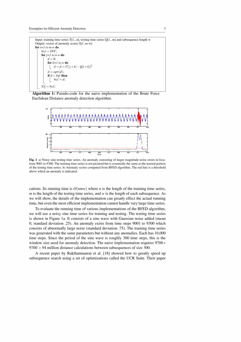
Algorithm 1: Pseudo-code for the naive implementation of the Brute ForceEuclidean Distance anomaly detection algorithm.

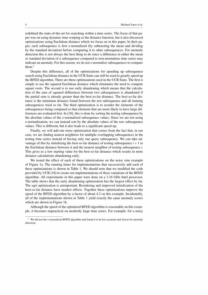
Fig. 1 a) Noisy sine testing time series. An anomaly consisting of larger magnitude noise exists in loca-tions 9001 to 9300. The training time series is not pictured but is essentially the same as the normal portionof the testing time series. b) Anomaly scores computed from BFED algorithm. The red line is a thresholdabove which an anomaly is indicated.

cations. Its running time is O(nmw) where n is the length of the training time series,m is the length of the testing time series, and w is the length of each subsequence. Aswe will show, the details of the implementation can greatly effect the actual runningtime, but even the most efficient implementation cannot handle very large time series.

To evaluate the running time of various implementations of the BFED algorithm,we will use a noisy sine time series for training and testing. The testing time seriesis shown in Figure 1a. It consists of a sine wave with Gaussian noise added (mean0, standard deviation .25). An anomaly exists from time steps 9001 to 9300 whichconsists of abnormally large noise (standard deviation .75). The training time serieswas generated with the same parameters but without any anomalies. Each has 10,000time steps. Since the period of the sine wave is roughly 300 time steps, this is thewindow size used for anomaly detection. The naive implementation requires 9700 ∗9700 > 94 million distance calculations between subsequences of size 300.

A recent paper by Rakthanmanon et al. [18] showed how to greatly speed upsubsequence search using a set of optimizations called the UCR Suite. Their paper


redefined the state-of-the-art for searching within a time series. The focus of that pa-per was on using dynamic time warping as the distance function, but it also discussedoptimizations using Euclidean distance which we focus on in this paper. In their pa-per, each subsequence is first z-normalized (by subtracting the mean and dividingby the standard deviation) before comparing it to other subsequences. For anomalydetection this is not always the best thing to do since a difference in either the meanor standard deviation of a subsequence compared to non-anomalous time series mayindicate an anomaly. For this reason, we do not z-normalize subsequences to comparethem.1

Despite this difference, all of the optimizations for speeding up subsequencesearch using Euclidean distance in the UCR Suite can still be used to greatly speed upthe BFED algorithm. There are three optimizations used in the UCR Suite. The first issimply to use the squared Euclidean distance which eliminates the need to computesquare roots. The second is to use early abandoning which means that the calcula-tion of the sum of squared differences between two subsequences is abandoned ifthe partial sum is already greater than the best-so-far distance. The best-so-far dis-tance is the minimum distance found between the test subsequence and all trainingsubsequences tried so far. The third optimization is to reorder the elements of thesubsequences being compared so that elements that are more likely to have large dif-ferences are evaluated first. In [18], this is done by sorting the testing subsequence bythe absolute values of the z-normalized subsequence values. Since we are not usingz-normalization, we can instead sort by the absolute values of the raw subsequencevalues. This is different, but it also leads to a significant speed-up.

Finally, we will add one more optimization that comes from the fact that, in ourcase, we are finding nearest neighbors for multiple overlapping subsequences in thetesting time series instead of having only one query subsequence. We can take ad-vantage of this by initializing the best-so-far distance of testing subsequence i+1 tothe Euclidean distance between it and the nearest neighbor of testing subsequence i.This gives us a low starting value for the best-so-far distance which results in moredistance calculations abandoning early.

We tested the effect of each of these optimizations on the noisy sine exampleof Figure 1a. The running times for implementations that successively add each ofthese optimizations is shown in Table 1. We should note that we modified the codeprovided by UCR [18] to create our implementations of these variations of the BFEDalgorithm. All experiments in this paper were done on a 3.16 GHz Intel processor.The table shows that the early abandoning optimization has the largest effect by far.The sqrt optimization is unimportant. Reordering and improved initialization of thebest-so-far distance have modest effects. Together these optimizations improve thespeed of the BFED algorithm by a factor of about 4.2 on this example. Incidentally,all of the implementations shown in Table 1 yield exactly the same anomaly scoreswhich are shown in Figure 1b.

Although the speed of the optimized BFED algorithm is reasonable on this exam-ple, it becomes impractical on modestly large time series. For example, for a noisy

1 We did test the z-normalized BFED algorithm and found it to be less accurate and slower for anomalydetection.


Method Run TimeBFED (no optimizations) 199.02 secBFED (no sqrt) 198.80 secBFED (no sqrt, early abandon) 53.98 secBFED (no sqrt, early abandon, reorder) 49.04 secBFED (no sqrt, early abandon, reorder, 46.96 secinitialization of best-so-far distance)

Table 1 Comparison of the running times of various implementations of brute force Euclidean distanceBFED anomaly detection.

sine problem with 1 million time steps for training and 10 million time steps for test-ing, the number of Euclidean distance calculations between subsequences is about10 trillion and the running time is about 51 days for the fully optimized BFED im-plementation. In the next sections we will present an anomaly detection algorithmthat can process this data in less then 4 minutes while improving on the accuracy ofBFED as well as reducing the memory requirements.

3 Exemplars for fast anomaly detection

For the problem of anomaly detection the location of the best matching training sub-sequence for each testing subsequence is not needed. Only the distance is necessary.This fact allows the possibility of replacing the training time series with a more com-pact summary of it. With this insight, we propose to replace the training time serieswith a set of exemplars that summarize all the subsequences in it. The first questionis what an exemplar should be. One possibility is for each exemplar to be simply adifferent raw subsequence of the training time series. The problem with this is thatvery many such exemplars would be needed to retain all of the variations present inthe training time series. Another possibility is for each exemplar to be an average ofsimilar subsequences. Averaging subsequences results in smoothing and the loss ofmost of the stochastic components (such as noise) of the subsequences. Each exem-plar would mainly retain the different trajectories present in the training data. The setof exemplars should ideally represent both the trajectories and the stochastic varia-tions present in the training subsequences. With this motivation we propose a repre-sentation of exemplars we call Statistical and Smoothed Trajectory (SST) features.This representation was also used in an earlier paper of ours on anomaly detection inmultidimensional time series [10].

We represent a subsequence as a trajectory component that captures the shapeof the time series within the window, and a statistical component that captures thestochastic component. These components can also be thought of roughly as the lowfrequency (trajectory) and high frequency (stochastic) components. The trajectorycomponent is computed using a simple fixed-window running average to yield asmoothed time series after subtracting the mean of the window. Because of smooth-ing, half of the values in the smoothed time series can be discarded without losingimportant information. Thus, the trajectory component has w/2 elements. See Figure2b. The statistical component is a small set of statistics computed over time series


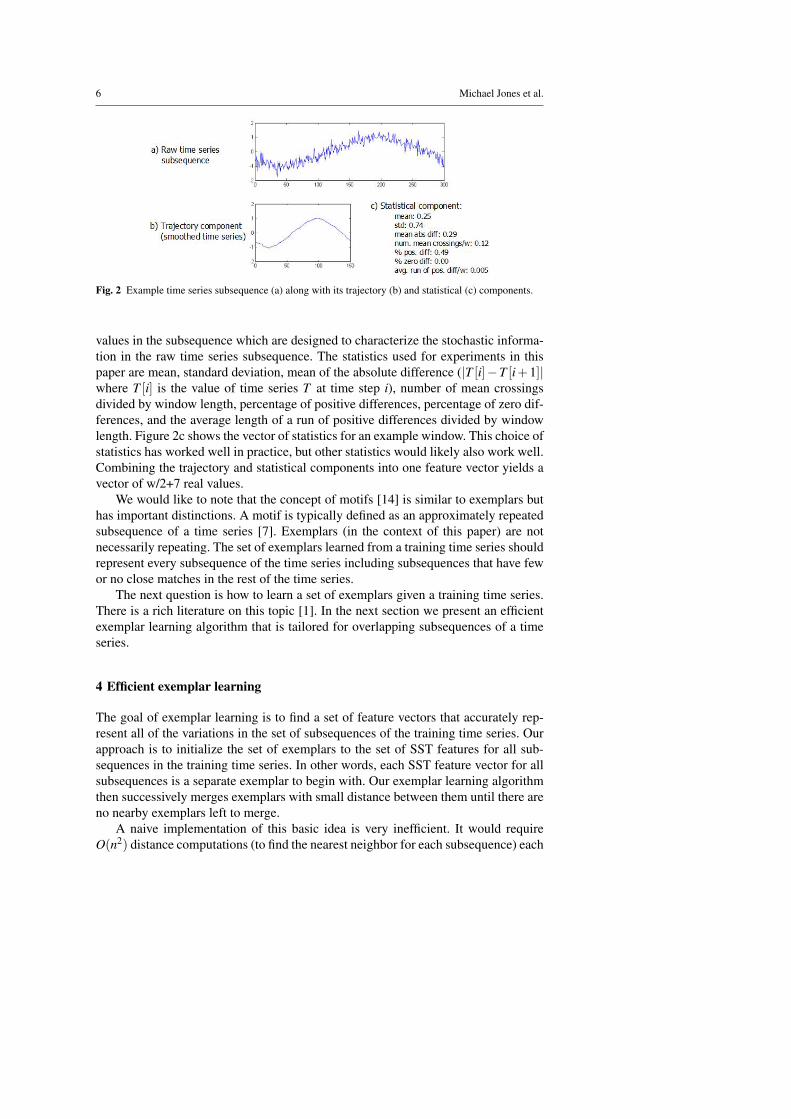
Fig. 2 Example time series subsequence (a) along with its trajectory (b) and statistical (c) components.

values in the subsequence which are designed to characterize the stochastic informa-tion in the raw time series subsequence. The statistics used for experiments in thispaper are mean, standard deviation, mean of the absolute difference (|T [i]−T [i+1]|where T [i] is the value of time series T at time step i), number of mean crossingsdivided by window length, percentage of positive differences, percentage of zero dif-ferences, and the average length of a run of positive differences divided by windowlength. Figure 2c shows the vector of statistics for an example window. This choice ofstatistics has worked well in practice, but other statistics would likely also work well.Combining the trajectory and statistical components into one feature vector yields avector of w/2+7 real values.

We would like to note that the concept of motifs [14] is similar to exemplars buthas important distinctions. A motif is typically defined as an approximately repeatedsubsequence of a time series [7]. Exemplars (in the context of this paper) are notnecessarily repeating. The set of exemplars learned from a training time series shouldrepresent every subsequence of the time series including subsequences that have fewor no close matches in the rest of the time series.

The next question is how to learn a set of exemplars given a training time series.There is a rich literature on this topic [1]. In the next section we present an efficientexemplar learning algorithm that is tailored for overlapping subsequences of a timeseries.

4 Efficient exemplar learning

The goal of exemplar learning is to find a set of feature vectors that accurately rep-resent all of the variations in the set of subsequences of the training time series. Ourapproach is to initialize the set of exemplars to the set of SST features for all sub-sequences in the training time series. In other words, each SST feature vector for allsubsequences is a separate exemplar to begin with. Our exemplar learning algorithmthen successively merges exemplars with small distance between them until there areno nearby exemplars left to merge.

A naive implementation of this basic idea is very inefficient. It would requireO(n2) distance computations (to find the nearest neighbor for each subsequence) each


of which is O(w) for a total of O(n2w). This is the same time complexity as the naiveBFED algorithm when the length of the training and testing time series are both n.We will present a hierarchical merging algorithm that runs in O(nw) for typical timeseries.

First, we need to define a distance between SST feature vectors v1 and v2. Giventhe success of the Euclidean distance for anomaly detection already discussed, wedefine the SST distance as the Euclidean distance between the trajectory componentsplus the Euclidean distance between the statistical components weighted by w/2

7 inorder to give equal weight to each component.

dist(v1,v2) =l

∑i=1

(v1.t(i)− v2.t(i))2 +l7

7

∑i=1

(v1.s(i)− v2.s(i))2 (1)

where v1 and v2 are two feature vectors, v j.t is the length l = w/2 trajectory compo-nent of v j, and v j.s is the length 7 statistical component of v j.

4.1 Initial merging

Based on the observation that overlapping subsequences often have small distancesbetween them, we reduce the size of the initial exemplar set by merging the SST fea-ture vectors of similar overlapping subsequences. To merge two SST feature vectorswe simply take a weighted average of the two vectors. The weight for each featurevector is the number of features vectors that have already been averaged into it. Thisweight is 1 for all of the initial exemplars and is the sum of the two weights whenfeature vectors are merged.

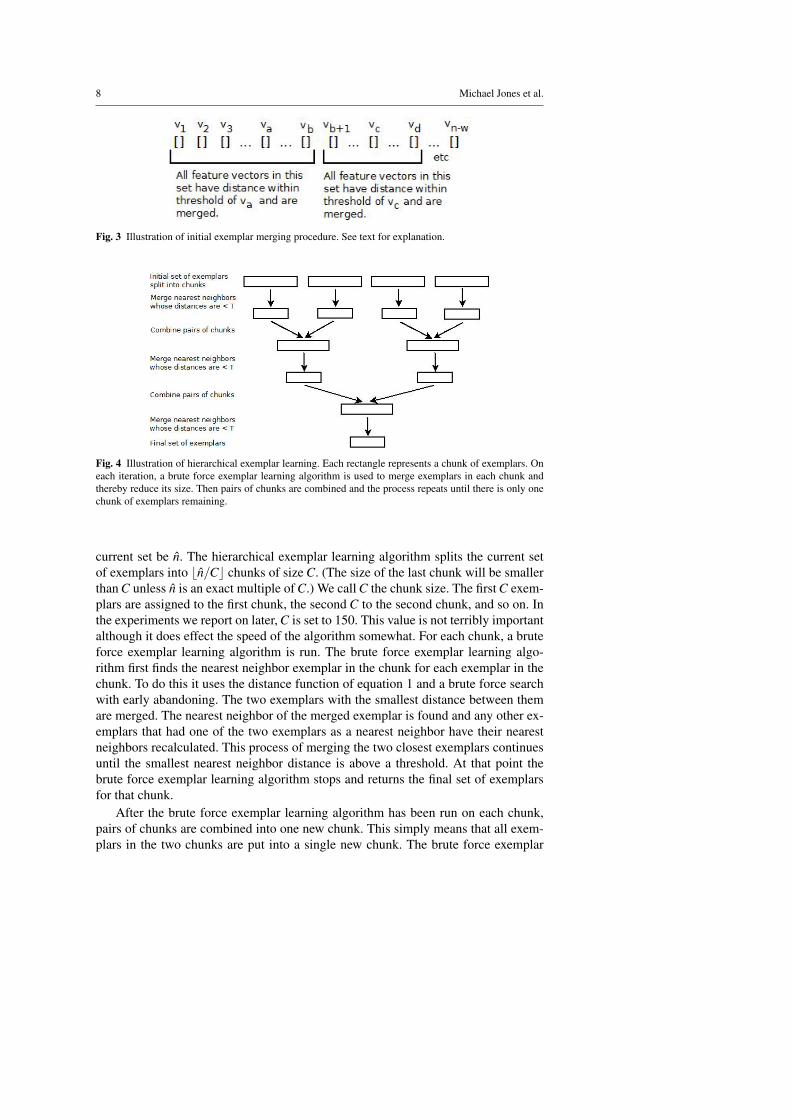
To explain the initial merging procedure in more detail, let us define vi as the fea-ture vector corresponding to subsequence T[i...i+w-1]. A threshold on the distance isneeded to determine whether two SST feature vectors are close enough. We describe amethod for automatically selecting this threshold in subsection 4.4. The initial merg-ing algorithm starts with feature vector v1 and computes the distance to successivefeature vectors until the distance is greater than the threshold. Let va be the last featurevector whose distance to v1 is below threshold. Then we continue searching forwardfor the furthest overlapping feature vector to va whose distance is below threshold.Call this feature vector vb. Feature vectors v1 through vb are then merged. This pro-cess is then repeated starting at the next feature vector vb+1. This initial merging ofoverlapping subsequences is fast (O(nw) since it only makes one pass over the set ofSST feature vectors) and typically results in about a 90% reduction in the number ofexemplars. Figure 3 illustates the initial merging procedure.

4.2 Hierarchical exemplar learning

After the initial merging phase, the resulting set of exemplars are passed to an hier-archical exemplar learning algorithm. The goal of this algorithm is to efficiently findand merge all similar exemplars (still represented by SST feature vectors) - not justones that represent overlapping subsequences. Let the number of exemplars in the


Fig. 3 Illustration of initial exemplar merging procedure. See text for explanation.

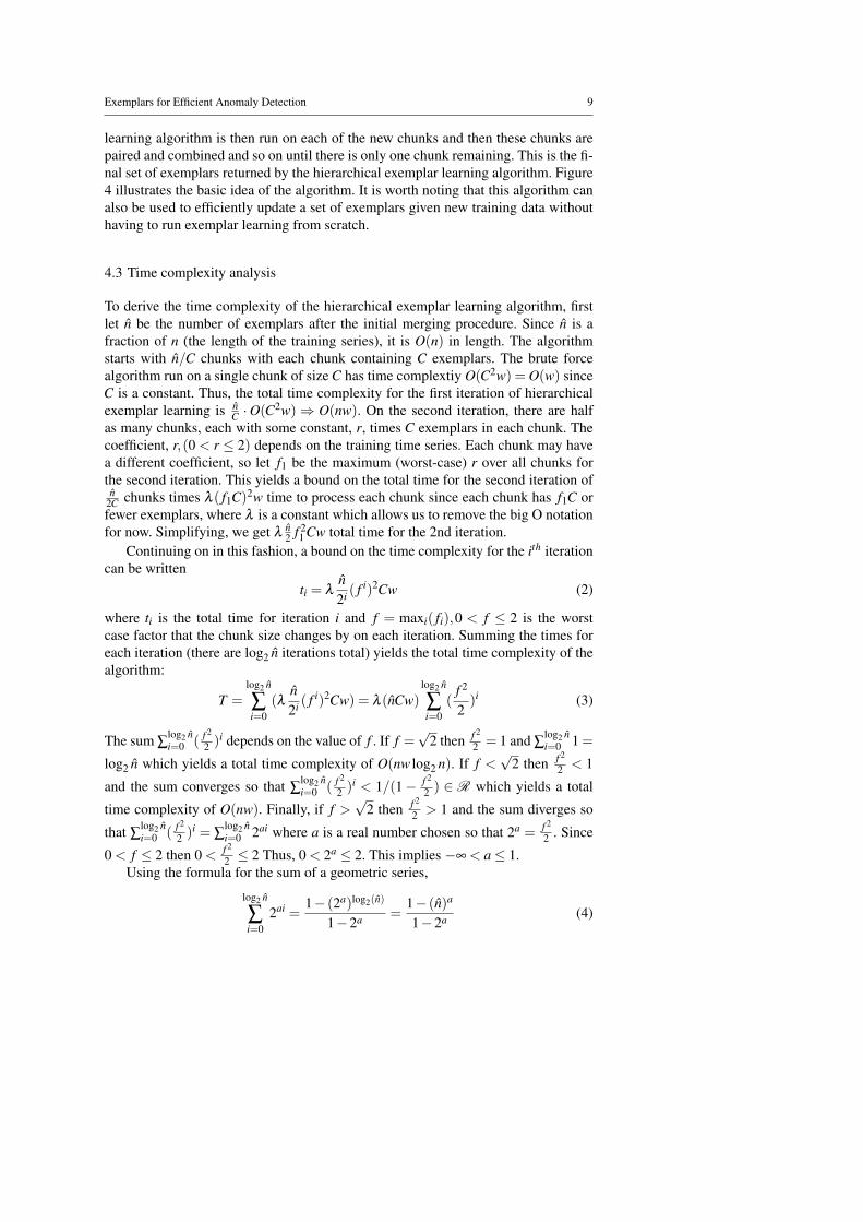
Fig. 4 Illustration of hierarchical exemplar learning. Each rectangle represents a chunk of exemplars. Oneach iteration, a brute force exemplar learning algorithm is used to merge exemplars in each chunk andthereby reduce its size. Then pairs of chunks are combined and the process repeats until there is only onechunk of exemplars remaining.

current set be n̂. The hierarchical exemplar learning algorithm splits the current setof exemplars into bn̂/Cc chunks of size C. (The size of the last chunk will be smallerthan C unless n̂ is an exact multiple of C.) We call C the chunk size. The first C exem-plars are assigned to the first chunk, the second C to the second chunk, and so on. Inthe experiments we report on later, C is set to 150. This value is not terribly importantalthough it does effect the speed of the algorithm somewhat. For each chunk, a bruteforce exemplar learning algorithm is run. The brute force exemplar learning algo-rithm first finds the nearest neighbor exemplar in the chunk for each exemplar in thechunk. To do this it uses the distance function of equation 1 and a brute force searchwith early abandoning. The two exemplars with the smallest distance between themare merged. The nearest neighbor of the merged exemplar is found and any other ex-emplars that had one of the two exemplars as a nearest neighbor have their nearestneighbors recalculated. This process of merging the two closest exemplars continuesuntil the smallest nearest neighbor distance is above a threshold. At that point thebrute force exemplar learning algorithm stops and returns the final set of exemplarsfor that chunk.

After the brute force exemplar learning algorithm has been run on each chunk,pairs of chunks are combined into one new chunk. This simply means that all exem-plars in the two chunks are put into a single new chunk. The brute force exemplar


learning algorithm is then run on each of the new chunks and then these chunks arepaired and combined and so on until there is only one chunk remaining. This is the fi-nal set of exemplars returned by the hierarchical exemplar learning algorithm. Figure4 illustrates the basic idea of the algorithm. It is worth noting that this algorithm canalso be used to efficiently update a set of exemplars given new training data withouthaving to run exemplar learning from scratch.

4.3 Time complexity analysis

To derive the time complexity of the hierarchical exemplar learning algorithm, firstlet n̂ be the number of exemplars after the initial merging procedure. Since n̂ is afraction of n (the length of the training series), it is O(n) in length. The algorithmstarts with n̂/C chunks with each chunk containing C exemplars. The brute forcealgorithm run on a single chunk of size C has time complextiy O(C2w) = O(w) sinceC is a constant. Thus, the total time complexity for the first iteration of hierarchicalexemplar learning is n̂

C ·O(C2w)⇒ O(nw). On the second iteration, there are halfas many chunks, each with some constant, r, times C exemplars in each chunk. Thecoefficient, r,(0 < r ≤ 2) depends on the training time series. Each chunk may havea different coefficient, so let f1 be the maximum (worst-case) r over all chunks forthe second iteration. This yields a bound on the total time for the second iteration ofn̂

2C chunks times λ ( f1C)2w time to process each chunk since each chunk has f1C orfewer exemplars, where λ is a constant which allows us to remove the big O notationfor now. Simplifying, we get λ

n̂2 f 2

1 Cw total time for the 2nd iteration.Continuing on in this fashion, a bound on the time complexity for the ith iteration

can be writtenti = λ

n̂2i ( f i)2Cw (2)

where ti is the total time for iteration i and f = maxi( fi),0 < f ≤ 2 is the worstcase factor that the chunk size changes by on each iteration. Summing the times foreach iteration (there are log2 n̂ iterations total) yields the total time complexity of thealgorithm:

T =log2 n̂

∑i=0

(λn̂2i ( f i)2Cw) = λ (n̂Cw)

log2 n̂

∑i=0

(f 2

2)i (3)

The sum ∑log2 n̂i=0 ( f 2

2 )i depends on the value of f . If f =√

2 then f 2

2 = 1 and ∑log2 n̂i=0 1 =

log2 n̂ which yields a total time complexity of O(nw log2 n). If f <√

2 then f 2

2 < 1

and the sum converges so that ∑log2 n̂i=0 ( f 2

2 )i < 1/(1− f 2

2 ) ∈ R which yields a total

time complexity of O(nw). Finally, if f >√

2 then f 2

2 > 1 and the sum diverges so

that ∑log2 n̂i=0 ( f 2

2 )i = ∑log2 n̂i=0 2ai where a is a real number chosen so that 2a = f 2

2 . Since

0 < f ≤ 2 then 0 < f 2

2 ≤ 2 Thus, 0 < 2a ≤ 2. This implies −∞ < a≤ 1.Using the formula for the sum of a geometric series,

log2 n̂

∑i=0

2ai =1− (2a)log2(n̂)

1−2a =1− (n̂)a

1−2a (4)


Time series length 103 104 105 106 107

Running time (sec) .05 .44 4.15 41.59 441.61

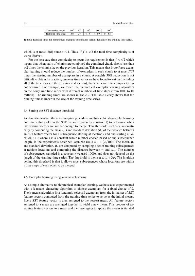
Table 2 Running times for hierarchical exemplar learning for various lengths of the training time series.

which is at most O(n̂) since a ≤ 1. Thus, if f >√

2 the total time complexity is atworst O(n2w).

For the best case time complexity to occur the requirement is that f <√

2 whichmeans that when pairs of chunks are combined the combined chunk size is less than√

2 times the chunk size on the previous iteration. This means that brute force exem-plar learning should reduce the number of exemplars in each chunk to at most .707times the starting number of exemplars in a chunk. A roughly 30% reduction is notdifficult to obtain. In practice, on every time series we have found to test on (includingall of the time series in the experimental section), the worst case time complexity hasnot occurred. For example, we tested the hierarchical exemplar learning algorithmon the noisy sine time series with different numbers of time steps (from 1000 to 10million). The running times are shown in Table 2. The table clearly shows that therunning time is linear in the size of the training time series.

4.4 Setting the SST distance threshold

As described earlier, the inital merging procedure and hierarchical exemplar learningboth use a threshold on the SST distance (given by equation 1) to determine whentwo feature vectors are similar enough to merge. This threshold is chosen automati-cally by computing the mean (µ) and standard deviation (σ ) of the distance betweenan SST feature vector for a subsequence starting at location i and one starting at lo-cation i+ s where s is a constant whole number chosen based on the subsequencelength. In the experiments described later, we use s = 1+(w/100). The mean, µ ,and standard deviation, σ , are computed by sampling a set of training subsequencesat random locations and computing the distance between vi and vi+s. The numberof subsequences sampled is a constant (we used 1000), and does not depend on thelength of the training time series. The threshold is then set to µ + 3σ . The intuitionbehind this threshold is that it allows most subsequences whose locations are withins time steps of each other to be merged.

4.5 Exemplar learning using k-means clustering

As a simple alternative to hierarchical exemplar learning, we have also experimentedwith a k-means clustering algorithm to choose exemplars for a fixed choice of k.The k-means algorithm first randomly selects k exemplars from the initial set of SSTfeature vectors computed from the training time series to serve as the initial means.Every SST feature vector is then assigned to the nearest mean. All feature vectorsassigned to a mean are averaged together to yield a new mean. This process of as-signing feature vectors to a mean and then averaging to update the means is iterated


a fixed number of times. We tested this simple algorithm on the 26 test sets describedin Section 6 with k set to 50 (which is the average number of exemplars chosen byour hierarchical exemplar learning algorithm on the test sets) and the number of it-erations set to 3. With these parameter settings, the accuracy of SST exemplars isslightly lower compared to hierarchical exemplar learning (detection rate of 42/45versus 44/45 on the 26 test sets from Section 6) with slightly slower overall speed(13.83 seconds versus 11.84 seconds for all of the test sets in Section 6). The accu-racy of k-means exemplar learning could be made to match that of hierarchical ex-emplar learning if a method of automatically optimizing k were used. However, thiswould make the k-means clustering algorithm much slower since multiple choicesfor k would need to be tested. Thus, k-means clustering is a reasonable alternative forexemplar learning, but appears to be unable to match the speed and accuracy of thehierarchical exemplar learning algorithm.

5 Anomaly detection with SST exemplars

After a set of exemplars have been learned to summarize the training time series, thereis one final step to finalize our model. Since each exemplar represents a set of similarSST features, we have not just a mean feature vector for each exemplar, but also astandard deviation for each component of the feature vector. The standard deviationis computed during exemplar learning by keeping track of the sum of squares of eachcomponent of each feature vector that is merged to form an exemplar. After exemplarlearning completes, we use the following formula to compute the standard deviationfor each component of the feature vector:

σ j =

√1N

N

∑i=1

(v2i j)−µ2

j (5)

where σ j is the standard deviation of the jth component of the exemplar, {vi} isthe set of SST feature vectors that were merged together to form this exemplar, N isthe number of such feature vectors, and µ j is the mean of the jth component of theexemplar.

Thus, each exemplar is represented by a mean SST feature vector (with w/2+7components) and a standard deviation for each component of the SST feature vector(also with w/2+7 components) for a total of w+14 real numbers to represent eachexemplar.

Computing the standard deviation for each component of the SST feature tellsus how much a test SST feature can deviate from an exemplar’s mean before thedeviation becomes unusual (i.e. not common in the training time series). Given thismotivation, we define a distance between a single SST feature vector, v (computedfrom a single time series subsequence) and an exemplar, e, that includes both meanand standard deviation components.

d(v,e) =l

∑i=1

max(0,|v.t(i)− e.t(i)|

e.σ(i)−3)


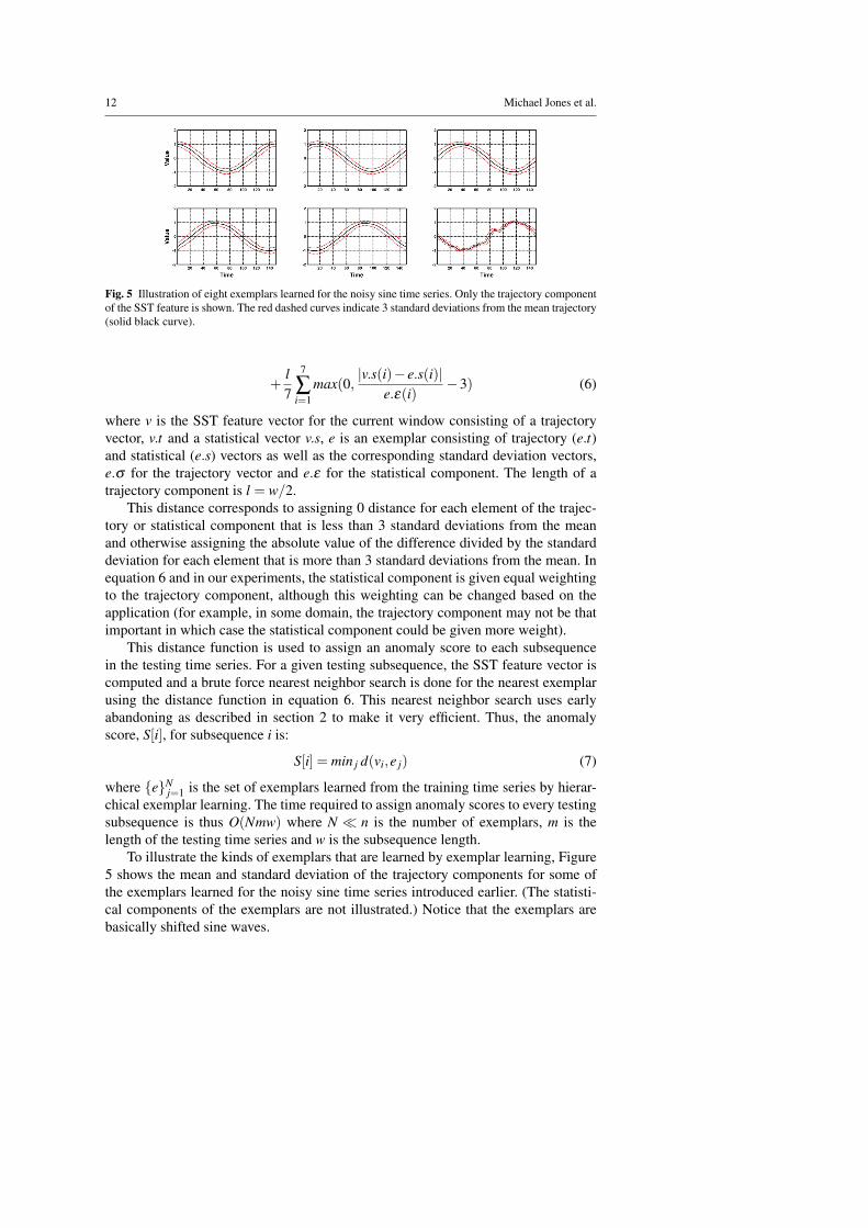
Fig. 5 Illustration of eight exemplars learned for the noisy sine time series. Only the trajectory componentof the SST feature is shown. The red dashed curves indicate 3 standard deviations from the mean trajectory(solid black curve).

+l7

7

∑i=1

max(0,|v.s(i)− e.s(i)|

e.ε(i)−3) (6)

where v is the SST feature vector for the current window consisting of a trajectoryvector, v.t and a statistical vector v.s, e is an exemplar consisting of trajectory (e.t)and statistical (e.s) vectors as well as the corresponding standard deviation vectors,e.σ for the trajectory vector and e.ε for the statistical component. The length of atrajectory component is l = w/2.

This distance corresponds to assigning 0 distance for each element of the trajec-tory or statistical component that is less than 3 standard deviations from the meanand otherwise assigning the absolute value of the difference divided by the standarddeviation for each element that is more than 3 standard deviations from the mean. Inequation 6 and in our experiments, the statistical component is given equal weightingto the trajectory component, although this weighting can be changed based on theapplication (for example, in some domain, the trajectory component may not be thatimportant in which case the statistical component could be given more weight).

This distance function is used to assign an anomaly score to each subsequencein the testing time series. For a given testing subsequence, the SST feature vector iscomputed and a brute force nearest neighbor search is done for the nearest exemplarusing the distance function in equation 6. This nearest neighbor search uses earlyabandoning as described in section 2 to make it very efficient. Thus, the anomalyscore, S[i], for subsequence i is:

S[i] = min j d(vi,e j) (7)

where {e}Nj=1 is the set of exemplars learned from the training time series by hierar-

chical exemplar learning. The time required to assign anomaly scores to every testingsubsequence is thus O(Nmw) where N � n is the number of exemplars, m is thelength of the testing time series and w is the subsequence length.

To illustrate the kinds of exemplars that are learned by exemplar learning, Figure5 shows the mean and standard deviation of the trajectory components for some ofthe exemplars learned for the noisy sine time series introduced earlier. (The statisti-cal components of the exemplars are not illustrated.) Notice that the exemplars arebasically shifted sine waves.


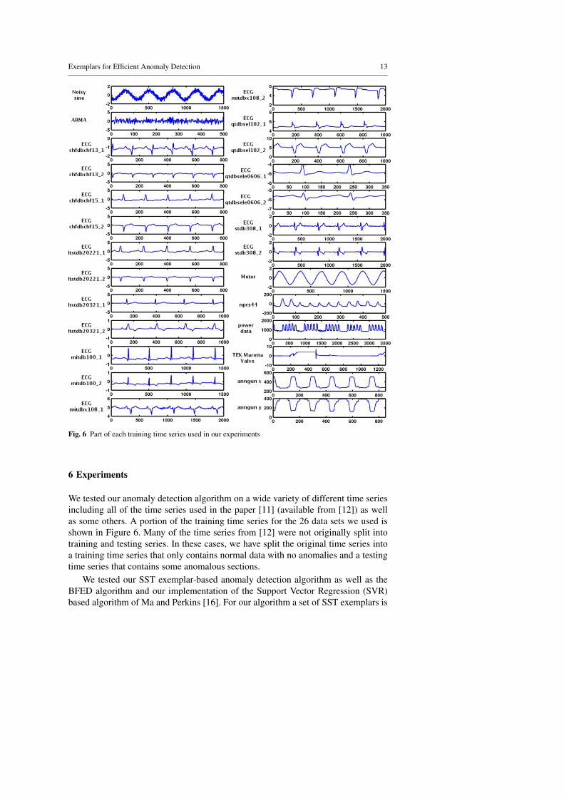
Fig. 6 Part of each training time series used in our experiments

6 Experiments

We tested our anomaly detection algorithm on a wide variety of different time seriesincluding all of the time series used in the paper [11] (available from [12]) as wellas some others. A portion of the training time series for the 26 data sets we used isshown in Figure 6. Many of the time series from [12] were not originally split intotraining and testing series. In these cases, we have split the original time series intoa training time series that only contains normal data with no anomalies and a testingtime series that contains some anomalous sections.

We tested our SST exemplar-based anomaly detection algorithm as well as theBFED algorithm and our implementation of the Support Vector Regression (SVR)based algorithm of Ma and Perkins [16]. For our algorithm a set of SST exemplars is


first learned on the training set as described in section 4 and then anomaly scores arecomputed for every subsequence of the testing set using the distance from equation 6as described in section 5. The same parameters (except for the subsequence length w)were used for all time series. A step size of 1 is used to advance from one subsequenceto the next so that consecutive subsequences overlap for all but their first and lastelements.

The SVR-based algorithm learns a linear combination of Gaussian functions us-ing Support Vector Regression to predict a value of the time series, T [i+w] given asubsequence, T [i, ..., i+w− 1]. This nonlinear function is learned from the trainingtime series and then used to predict each value of the testing time series. The anomalyscore is the squared difference between the prediction and the observed value.

The subsequence length, w, is chosen manually and is the main parameter of all ofthe algorithms. None of the algorithms is very sensitive to the choice of w althoughits choice can effect the type of anomalies that can be detected. For periodic timeseries, choosing w to be roughly the length of the period works well.

We compute detection rates for various false positive rates across all testing timeseries. The false positive rate is the fraction of non-anomalous subsequences that areabove threshold. The detection rate is the fraction of anomalous regions (not subse-quences) of a time series that are detected as anomalous. An anomalous region isconsidered to be detected if at least one subsequence in the region has an anomalyscore above threshold. This convention reflects the fact that in practice it is not im-portant that every subsequence within an imprecisely labeled anomalous region bedetected as anomalous. What is important is that at least one high anomaly score oc-curs in an anomalous region. A receiver operating characteristic (ROC) curve acrossall testing time series is computed by computing total detections over total anomaliesfor a fixed false positive rate for each testing time series.

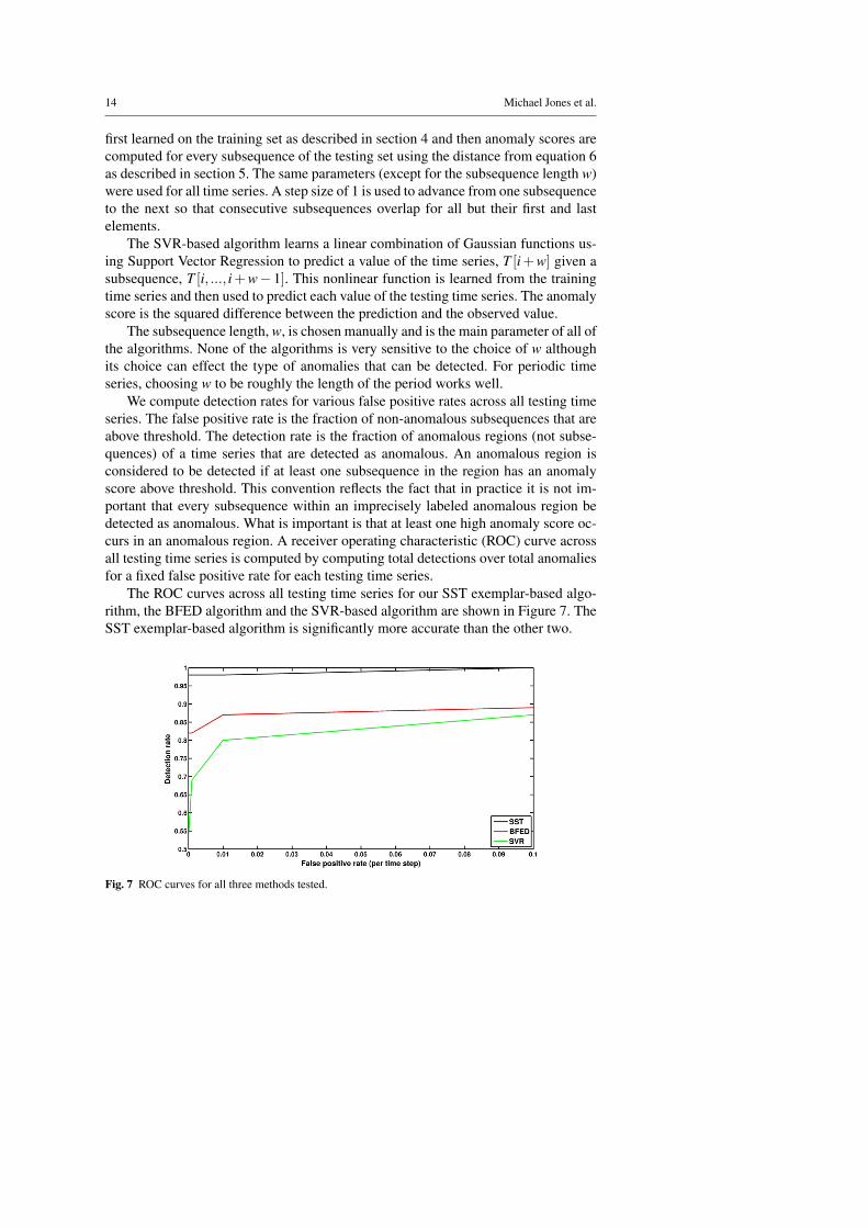
The ROC curves across all testing time series for our SST exemplar-based algo-rithm, the BFED algorithm and the SVR-based algorithm are shown in Figure 7. TheSST exemplar-based algorithm is significantly more accurate than the other two.

Fig. 7 ROC curves for all three methods tested.


Data set SST exemplars BFED SVRName Train, Det. Det. Det.

test length w N rate rate ratenoisy sine 10000, 10000 300 49 4/4 1/4 4/4ARMA 10000, 100000 100 12 2/2 0/2 0/2chfdbchf13 1 1875, 1875 160 17 1/1 1/1 1/1chfdbchf13 2 1875, 1875 160 17 1/1 1/1 1/1chfdbchf15 1 7500, 7500 160 72 1/1 1/1 0/1chfdbchf15 2 7500, 7500 160 23 1/1 1/1 0/1ltstdb20221 1 1875, 1875 160 24 1/1 0/1 1/1ltstdb20221 2 1875, 1875 160 24 1/1 1/1 0/1ltstdb20321 1 1875, 1875 200 23 1/1 1/1 0/1ltstdb20321 2 1875, 1875 200 31 1/1 1/1 1/1mitdb100 1 2700, 2700 300 36 1/1 1/1 0/1mitdb100 2 2700, 2700 300 102 1/1 1/1 0/1mitdbx108 1 5000, 5000 400 71 1/1 0/1 0/1mitdbx108 2 5000, 5000 400 114 1/1 0/1 0/1qtdbsel102 1 22500, 22500 200 156 1/1 1/1 1/1qtdbsel102 2 22500, 22500 200 38 1/1 1/1 1/1qtdbsel0606 1 700, 2300 70 15 1/1 1/1 1/1qtdbsel0606 2 700, 2300 70 19 1/1 1/1 1/1stdb308 1 2400, 3000 400 58 1/1 1/1 0/1stdb308 2 2400, 3000 400 53 1/1 1/1 1/1motor 7500, 30000 300 63 10/10 10/10 10/10nprs44 2000, 4500 100 61 1/1 1/1 1/1power data 1 11000, 15000 700 80 4/4 4/4 0/4power data 2 11000, 9040 700 80 0/1 1/1 0/1TEK 5901, 9099 256 79 3/3 3/3 0/3anngun x 5625,5625 170 33 1/1 1/1 0/1anngun y 5625,5625 170 39 1/1 1/1 0/1Totals 150501, N.A. 1309 44/45 37/45 24/45

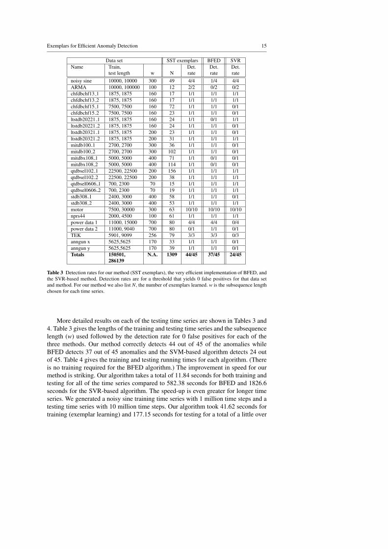
286139

Table 3 Detection rates for our method (SST exemplars), the very efficient implementation of BFED, andthe SVR-based method. Detection rates are for a threshold that yields 0 false positives for that data setand method. For our method we also list N, the number of exemplars learned. w is the subsequence lengthchosen for each time series.

More detailed results on each of the testing time series are shown in Tables 3 and4. Table 3 gives the lengths of the training and testing time series and the subsequencelength (w) used followed by the detection rate for 0 false positives for each of thethree methods. Our method correctly detects 44 out of 45 of the anomalies whileBFED detects 37 out of 45 anomalies and the SVM-based algorithm detects 24 outof 45. Table 4 gives the training and testing running times for each algorithm. (Thereis no training required for the BFED algorithm.) The improvement in speed for ourmethod is striking. Our algorithm takes a total of 11.84 seconds for both training andtesting for all of the time series compared to 582.38 seconds for BFED and 1826.6seconds for the SVR-based algorithm. The speed-up is even greater for longer timeseries. We generated a noisy sine training time series with 1 million time steps and atesting time series with 10 million time steps. Our algorithm took 41.62 seconds fortraining (exemplar learning) and 177.15 seconds for testing for a total of a little over


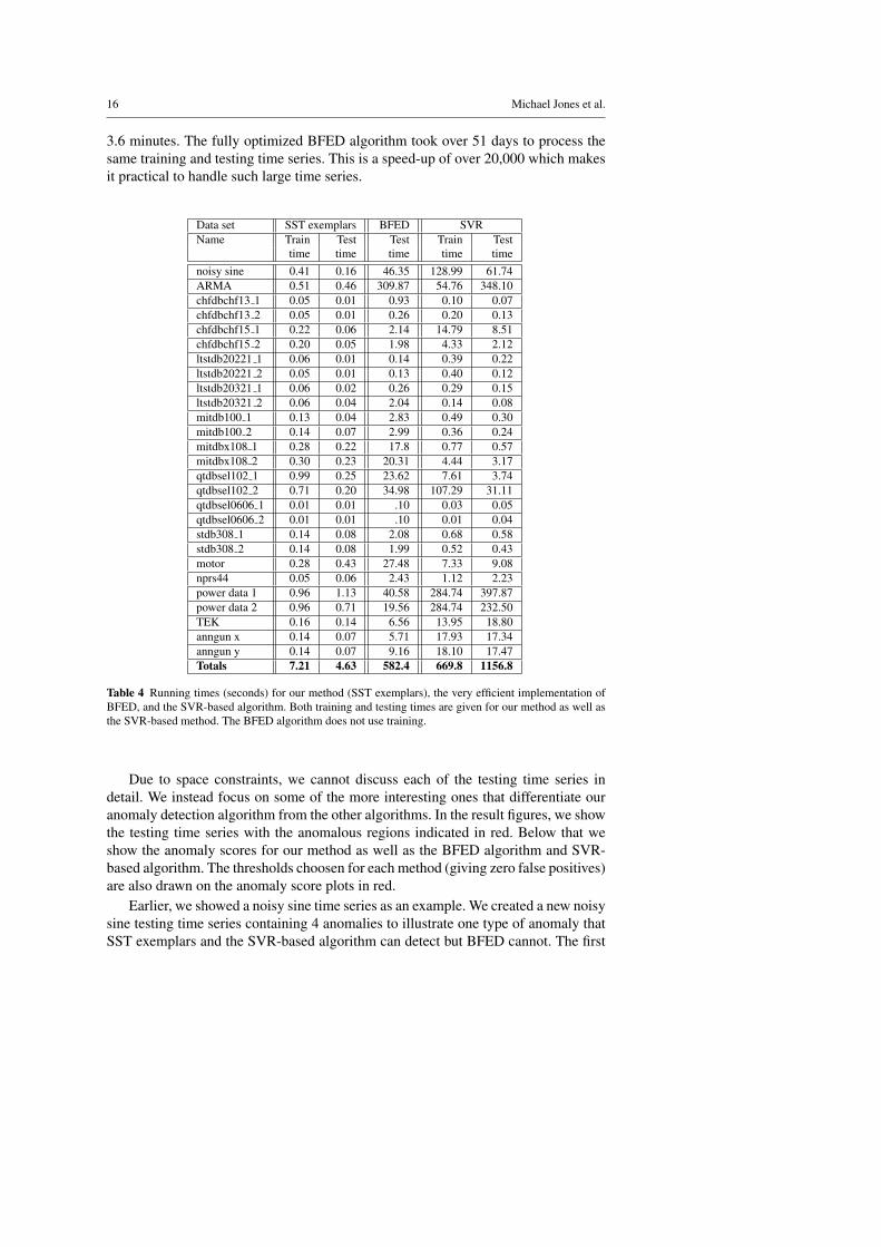
3.6 minutes. The fully optimized BFED algorithm took over 51 days to process thesame training and testing time series. This is a speed-up of over 20,000 which makesit practical to handle such large time series.

Data set SST exemplars BFED SVRName Train Test Test Train Test

time time time time timenoisy sine 0.41 0.16 46.35 128.99 61.74ARMA 0.51 0.46 309.87 54.76 348.10chfdbchf13 1 0.05 0.01 0.93 0.10 0.07chfdbchf13 2 0.05 0.01 0.26 0.20 0.13chfdbchf15 1 0.22 0.06 2.14 14.79 8.51chfdbchf15 2 0.20 0.05 1.98 4.33 2.12ltstdb20221 1 0.06 0.01 0.14 0.39 0.22ltstdb20221 2 0.05 0.01 0.13 0.40 0.12ltstdb20321 1 0.06 0.02 0.26 0.29 0.15ltstdb20321 2 0.06 0.04 2.04 0.14 0.08mitdb100 1 0.13 0.04 2.83 0.49 0.30mitdb100 2 0.14 0.07 2.99 0.36 0.24mitdbx108 1 0.28 0.22 17.8 0.77 0.57mitdbx108 2 0.30 0.23 20.31 4.44 3.17qtdbsel102 1 0.99 0.25 23.62 7.61 3.74qtdbsel102 2 0.71 0.20 34.98 107.29 31.11qtdbsel0606 1 0.01 0.01 .10 0.03 0.05qtdbsel0606 2 0.01 0.01 .10 0.01 0.04stdb308 1 0.14 0.08 2.08 0.68 0.58stdb308 2 0.14 0.08 1.99 0.52 0.43motor 0.28 0.43 27.48 7.33 9.08nprs44 0.05 0.06 2.43 1.12 2.23power data 1 0.96 1.13 40.58 284.74 397.87power data 2 0.96 0.71 19.56 284.74 232.50TEK 0.16 0.14 6.56 13.95 18.80anngun x 0.14 0.07 5.71 17.93 17.34anngun y 0.14 0.07 9.16 18.10 17.47Totals 7.21 4.63 582.4 669.8 1156.8

Table 4 Running times (seconds) for our method (SST exemplars), the very efficient implementation ofBFED, and the SVR-based algorithm. Both training and testing times are given for our method as well asthe SVR-based method. The BFED algorithm does not use training.

Due to space constraints, we cannot discuss each of the testing time series indetail. We instead focus on some of the more interesting ones that differentiate ouranomaly detection algorithm from the other algorithms. In the result figures, we showthe testing time series with the anomalous regions indicated in red. Below that weshow the anomaly scores for our method as well as the BFED algorithm and SVR-based algorithm. The thresholds choosen for each method (giving zero false positives)are also drawn on the anomaly score plots in red.

Earlier, we showed a noisy sine time series as an example. We created a new noisysine testing time series containing 4 anomalies to illustrate one type of anomaly thatSST exemplars and the SVR-based algorithm can detect but BFED cannot. The first


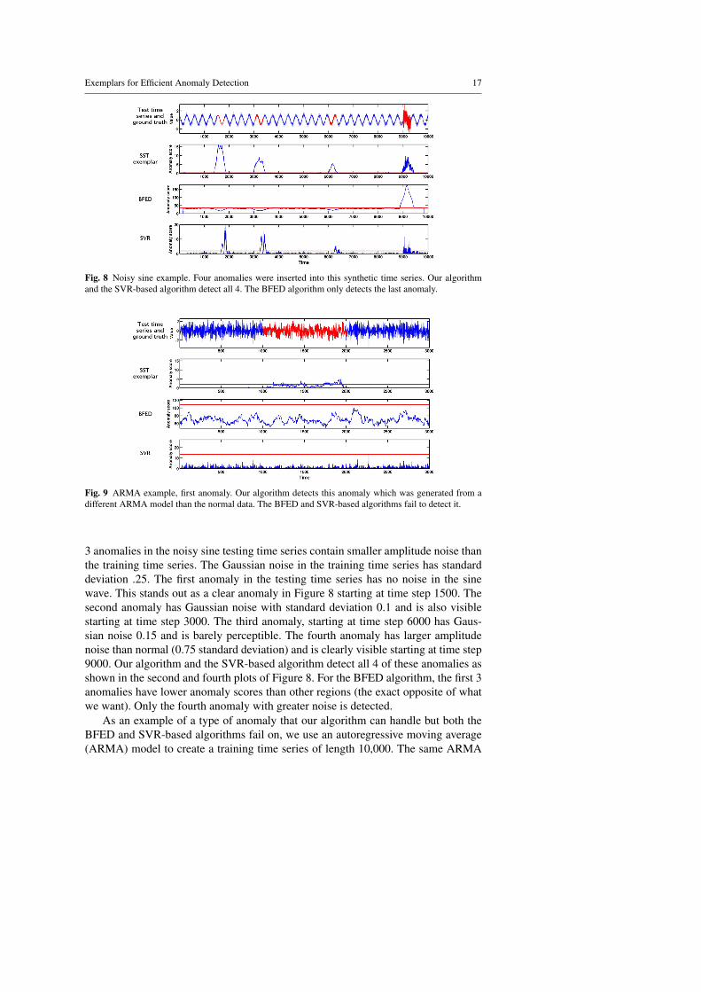
Fig. 8 Noisy sine example. Four anomalies were inserted into this synthetic time series. Our algorithmand the SVR-based algorithm detect all 4. The BFED algorithm only detects the last anomaly.

Fig. 9 ARMA example, first anomaly. Our algorithm detects this anomaly which was generated from adifferent ARMA model than the normal data. The BFED and SVR-based algorithms fail to detect it.

3 anomalies in the noisy sine testing time series contain smaller amplitude noise thanthe training time series. The Gaussian noise in the training time series has standarddeviation .25. The first anomaly in the testing time series has no noise in the sinewave. This stands out as a clear anomaly in Figure 8 starting at time step 1500. Thesecond anomaly has Gaussian noise with standard deviation 0.1 and is also visiblestarting at time step 3000. The third anomaly, starting at time step 6000 has Gaus-sian noise 0.15 and is barely perceptible. The fourth anomaly has larger amplitudenoise than normal (0.75 standard deviation) and is clearly visible starting at time step9000. Our algorithm and the SVR-based algorithm detect all 4 of these anomalies asshown in the second and fourth plots of Figure 8. For the BFED algorithm, the first 3anomalies have lower anomaly scores than other regions (the exact opposite of whatwe want). Only the fourth anomaly with greater noise is detected.

As an example of a type of anomaly that our algorithm can handle but both theBFED and SVR-based algorithms fail on, we use an autoregressive moving average(ARMA) model to create a training time series of length 10,000. The same ARMA


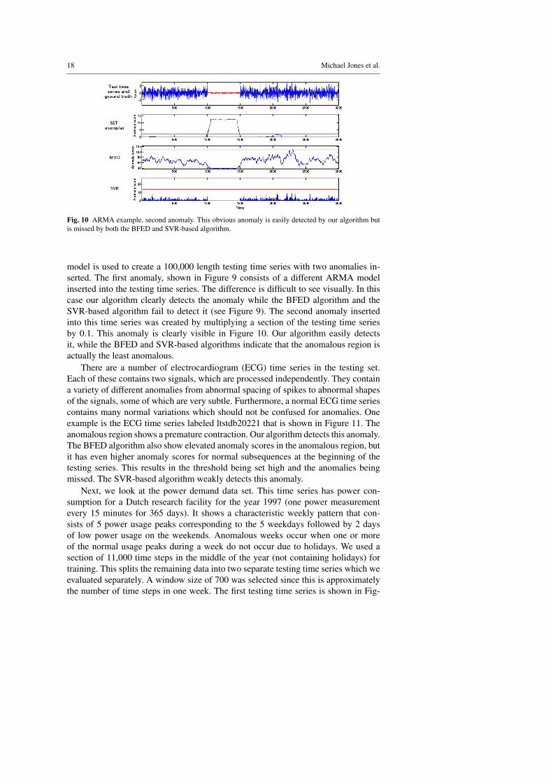
Fig. 10 ARMA example, second anomaly. This obvious anomaly is easily detected by our algorithm butis missed by both the BFED and SVR-based algorithm.

model is used to create a 100,000 length testing time series with two anomalies in-serted. The first anomaly, shown in Figure 9 consists of a different ARMA modelinserted into the testing time series. The difference is difficult to see visually. In thiscase our algorithm clearly detects the anomaly while the BFED algorithm and theSVR-based algorithm fail to detect it (see Figure 9). The second anomaly insertedinto this time series was created by multiplying a section of the testing time seriesby 0.1. This anomaly is clearly visible in Figure 10. Our algorithm easily detectsit, while the BFED and SVR-based algorithms indicate that the anomalous region isactually the least anomalous.

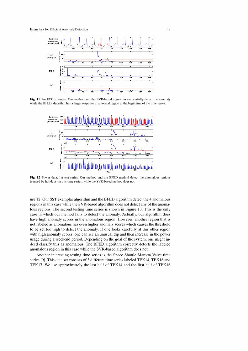
There are a number of electrocardiogram (ECG) time series in the testing set.Each of these contains two signals, which are processed independently. They containa variety of different anomalies from abnormal spacing of spikes to abnormal shapesof the signals, some of which are very subtle. Furthermore, a normal ECG time seriescontains many normal variations which should not be confused for anomalies. Oneexample is the ECG time series labeled ltstdb20221 that is shown in Figure 11. Theanomalous region shows a premature contraction. Our algorithm detects this anomaly.The BFED algorithm also show elevated anomaly scores in the anomalous region, butit has even higher anomaly scores for normal subsequences at the beginning of thetesting series. This results in the threshold being set high and the anomalies beingmissed. The SVR-based algorithm weakly detects this anomaly.

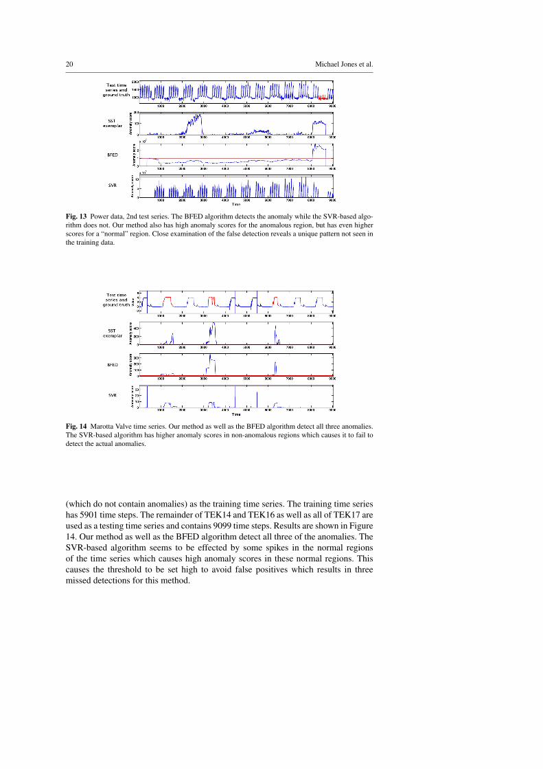
Next, we look at the power demand data set. This time series has power con-sumption for a Dutch research facility for the year 1997 (one power measurementevery 15 minutes for 365 days). It shows a characteristic weekly pattern that con-sists of 5 power usage peaks corresponding to the 5 weekdays followed by 2 daysof low power usage on the weekends. Anomalous weeks occur when one or moreof the normal usage peaks during a week do not occur due to holidays. We used asection of 11,000 time steps in the middle of the year (not containing holidays) fortraining. This splits the remaining data into two separate testing time series which weevaluated separately. A window size of 700 was selected since this is approximatelythe number of time steps in one week. The first testing time series is shown in Fig-


Fig. 11 An ECG example. Our method and the SVR-based algorithm successfully detect the anomalywhile the BFED algorithm has a larger response in a normal region at the beginning of the time series.

Fig. 12 Power data, 1st test series. Our method and the BFED method detect the anomalous regions(caused by holidays) in this time series, while the SVR-based method does not.

ure 12. Our SST exemplar algorithm and the BFED algorithm detect the 4 anomalousregions in this case while the SVR-based algorithm does not detect any of the anoma-lous regions. The second testing time series is shown in Figure 13. This is the onlycase in which our method fails to detect the anomaly. Actually, our algorithm doeshave high anomaly scores in the anomalous region. However, another region that isnot labeled as anomalous has even higher anomaly scores which causes the thresholdto be set too high to detect the anomaly. If one looks carefully at this other regionwith high anomaly scores, one can see an unusual dip and then increase in the powerusage during a weekend period. Depending on the goal of the system, one might in-deed classify this as anomalous. The BFED algorithm correctly detects the labeledanomalous region in this case while the SVR-based algorithm does not.

Another interesting testing time series is the Space Shuttle Marotta Valve timeseries [9]. This data set consists of 3 different time series labeled TEK14, TEK16 andTEK17. We use approximately the last half of TEK14 and the first half of TEK16


Fig. 13 Power data, 2nd test series. The BFED algorithm detects the anomaly while the SVR-based algo-rithm does not. Our method also has high anomaly scores for the anomalous region, but has even higherscores for a “normal” region. Close examination of the false detection reveals a unique pattern not seen inthe training data.

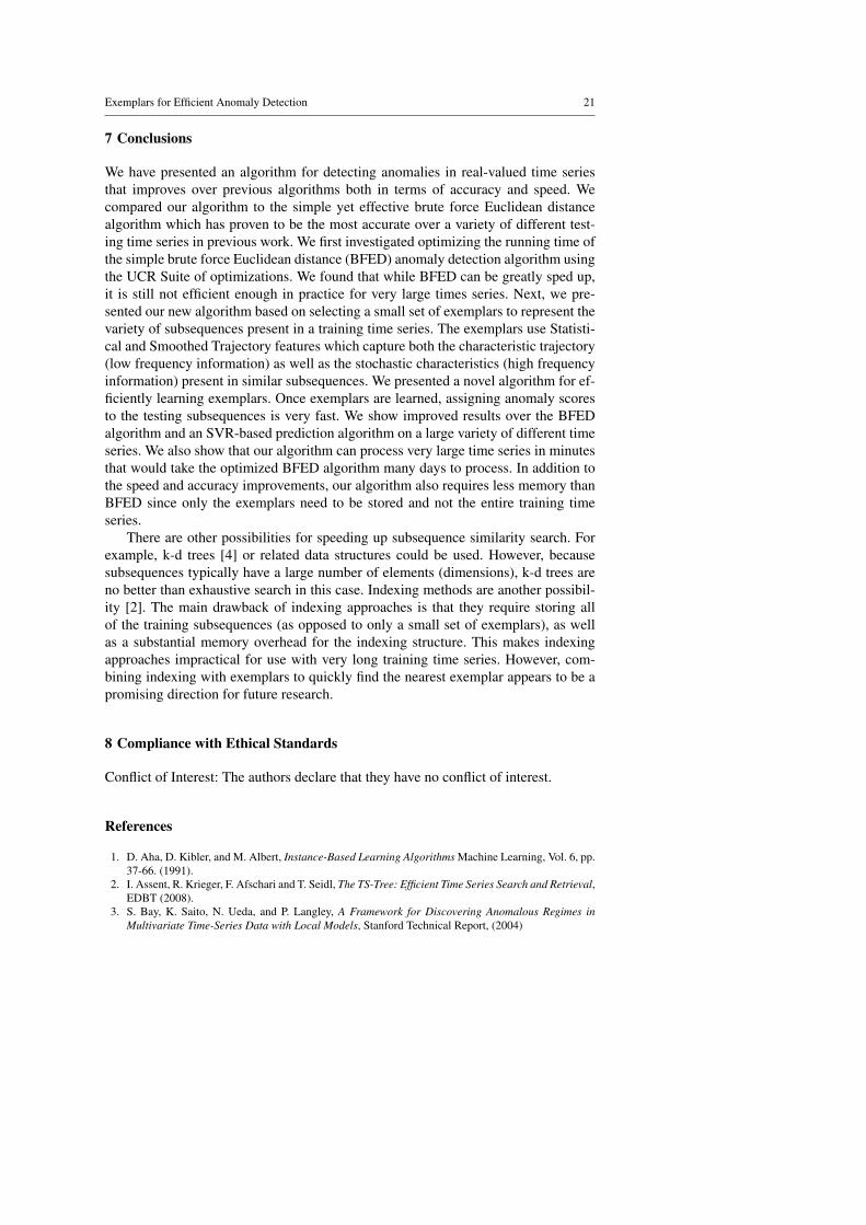
Fig. 14 Marotta Valve time series. Our method as well as the BFED algorithm detect all three anomalies.The SVR-based algorithm has higher anomaly scores in non-anomalous regions which causes it to fail todetect the actual anomalies.

(which do not contain anomalies) as the training time series. The training time serieshas 5901 time steps. The remainder of TEK14 and TEK16 as well as all of TEK17 areused as a testing time series and contains 9099 time steps. Results are shown in Figure14. Our method as well as the BFED algorithm detect all three of the anomalies. TheSVR-based algorithm seems to be effected by some spikes in the normal regionsof the time series which causes high anomaly scores in these normal regions. Thiscauses the threshold to be set high to avoid false positives which results in threemissed detections for this method.


7 Conclusions

We have presented an algorithm for detecting anomalies in real-valued time seriesthat improves over previous algorithms both in terms of accuracy and speed. Wecompared our algorithm to the simple yet effective brute force Euclidean distancealgorithm which has proven to be the most accurate over a variety of different test-ing time series in previous work. We first investigated optimizing the running time ofthe simple brute force Euclidean distance (BFED) anomaly detection algorithm usingthe UCR Suite of optimizations. We found that while BFED can be greatly sped up,it is still not efficient enough in practice for very large times series. Next, we pre-sented our new algorithm based on selecting a small set of exemplars to represent thevariety of subsequences present in a training time series. The exemplars use Statisti-cal and Smoothed Trajectory features which capture both the characteristic trajectory(low frequency information) as well as the stochastic characteristics (high frequencyinformation) present in similar subsequences. We presented a novel algorithm for ef-ficiently learning exemplars. Once exemplars are learned, assigning anomaly scoresto the testing subsequences is very fast. We show improved results over the BFEDalgorithm and an SVR-based prediction algorithm on a large variety of different timeseries. We also show that our algorithm can process very large time series in minutesthat would take the optimized BFED algorithm many days to process. In addition tothe speed and accuracy improvements, our algorithm also requires less memory thanBFED since only the exemplars need to be stored and not the entire training timeseries.

There are other possibilities for speeding up subsequence similarity search. Forexample, k-d trees [4] or related data structures could be used. However, becausesubsequences typically have a large number of elements (dimensions), k-d trees areno better than exhaustive search in this case. Indexing methods are another possibil-ity [2]. The main drawback of indexing approaches is that they require storing allof the training subsequences (as opposed to only a small set of exemplars), as wellas a substantial memory overhead for the indexing structure. This makes indexingapproaches impractical for use with very long training time series. However, com-bining indexing with exemplars to quickly find the nearest exemplar appears to be apromising direction for future research.

8 Compliance with Ethical Standards

Conflict of Interest: The authors declare that they have no conflict of interest.

References

1. D. Aha, D. Kibler, and M. Albert, Instance-Based Learning Algorithms Machine Learning, Vol. 6, pp.37-66. (1991).

2. I. Assent, R. Krieger, F. Afschari and T. Seidl, The TS-Tree: Efficient Time Series Search and Retrieval,EDBT (2008).

3. S. Bay, K. Saito, N. Ueda, and P. Langley, A Framework for Discovering Anomalous Regimes inMultivariate Time-Series Data with Local Models, Stanford Technical Report, (2004)


4. J. Bentley, Multidimensional binary search trees used for associative searching, Comm. of the ACM,18(9) (1975)

5. V. Chandola, A. Banerjee, and V. Kumar, Anomaly Detection: A Survey, ACM Computing Surveys,Vol. 41, No. 3, (2009).

6. V. Chandola, D. Cheboli, and V. Kumar, Detecting Anomalies in a Time Series Database, Dept. ofComputer Science and Engineering, Univ. of Minnesota Technical Report, TR 09-004 (2009).

7. B. Chiu, and E. Keogh, and S. Lonardi, Probabilistic Discovery of Time Series Motifs, SIGKDD(2003).

8. D. Dasgupta and S. Forrest, Novelty Detection in Time Series Data using Ideas from Immunology, 5thInt. Conf. on Intelligent Systems, (1996).

9. B. Farrell and S. Santuro, NASA Shuttle Valve Data, http://www.cs.fit.edu/∼pkc/nasa/data/ (2005).10. M. Jones and D. Nikovski and M. Imamura and T. Hirata, Anomaly Detection in Real-Valued Multi-

dimensional Time Series, Proceedings of the 2nd International ASE Conference on Big Data Scienceand Computing (2014).

11. E. Keogh, and J. Lin, and A. Fu, HOT SAX: Finding the Most Unusual Time Series Subsequence:Algorithms and Applications, ICDM (2005).

12. E. Keogh (2005). www.cs.ucr.edu/∼eamonn/discords/13. E. Koskivaara, Artificial Neural Network Models for Predicting Patterns in Auditing Monthly Bal-

ances, J. of the Operational Research Soc., Vol. 51 (1996).14. J. Lin, and E. Keogh, and S. Lonardi, and P. Patel, Finding Motifs in Time Series, SIGKDD (2002).15. B. Liu, H. Chen, A. Sharma, G. Jiang, and H. Xiong, Modeling Heterogeneous Time Series Dynamics

to Profile Big Sensor Data in Complex Physical Systems, IEEE Int. Conf. on Big Data (2013).16. J. Ma and S. Perkins, Online Novelty Detection on Temporal Sequences, SIGKDD (2003).17. M. Mahoney and P. Chan, Trajectory Boundary Modeling of Time Series for Anomaly Detection,

Workshop on Data Mining Methods for Anomaly Detection at KDD (2005).18. T. Rakthanmanon, B. Campana, A. Mueen, G. Batista, B. Westover, Q. Zhu, J. Zakaria, and E. Keogh,

Searching and Mining Trillions of Time Series Subsequences under Dynamic Time Warping, KDD(2012).

19. A. Rusiecki, Robust neural network for novelty detection on data streams, Int. Conf. on ArtificialIntelligence and Soft Computing (ICAISC) (2012).

20. C. Shahabi, X. Tian, and W. Zhao, TSA-tree: A Wavelet-Based Approach to Improve the Efficiency ofMulti-Level Surprise and Trend Queries on Time-Series Data, 12th International Conf. on Scientificand Statistical Database Management (SSDBM), (2000).

21. A. Ypma and R. Duin, Novelty detection using Self-Organizing Maps, In Proc. of ICONIP (1997).

Documents

Exemplar Learning for Extremely Efficient Anomaly