Embed Size (px)
Citation preview
Exemplar Guided Active Learning
Jason HartfordAI21 Labs
Kevin Leyton-BrownAI21 Labs
Hadas RavivAI21 Labs
Dan PadnosAI21 Labs
Shahar LevAI21 Labs
Barak LenzAI21 Labs
Abstract
We consider the problem of wisely using a limited budget to label a small subset ofa large unlabeled dataset. We are motivated by the NLP problem of word sensedisambiguation. For any word, we have a set of candidate labels from a knowledgebase, but the label set is not necessarily representative of what occurs in the data:there may exist labels in the knowledge base that very rarely occur in the corpusbecause the sense is rare in modern English; and conversely there may exist truelabels that do not exist in our knowledge base. Our aim is to obtain a classifierthat performs as well as possible on examples of each “common class” that occurswith frequency above a given threshold in the unlabeled set while annotating asfew examples as possible from “rare classes” whose labels occur with less than thisfrequency. The challenge is that we are not informed which labels are commonand which are rare, and the true label distribution may exhibit extreme skew. Wedescribe an active learning approach that (1) explicitly searches for rare classes byleveraging the contextual embedding spaces provided by modern language models,and (2) incorporates a stopping rule that ignores classes once we prove that theyoccur below our target threshold with high probability. We prove that our algorithmonly costs logarithmically more than a hypothetical approach that knows all truelabel frequencies and show experimentally that incorporating automated search cansignificantly reduce the number of samples needed to reach target accuracy levels.
1 Introduction
We are motivated by the problem of labelling a dataset for word sense disambiguation, where wewant to use a limited budget to collect annotations for a reasonable number of examples of eachsense for each word. This task can be thought of as an active learning problem (Settles, 2012), butwith two nonstandard challenges. First, for any given word we can get a set of candidate labels froma knowledge base such as WordNet (Fellbaum, 1998). However, this label set is not necessarilyrepresentative of what occurs in the data: there may exist labels in the knowledge base that do notoccur in the corpus because the sense is rare in modern English; conversely, there may also existtrue labels that do not exist in our knowledge base. For example, consider the word “bass.” It isfrequently used as a noun or modifier, e.g., “the bass and alto are good singers”, or “I play the bass
guitar”. It is also commonly used to refer to a type of fish, but because music is so widely discussedonline, the fish sense of the word is orders of magnitude less common than the low-frequency soundsense in internet text. The Oxford dictionary (Lexico) also notes that bass once referred to a fibrousmaterial used in matting or chords, but that sense is not common in modern English. We want amethod that collects balanced labels for the common senses, “bass frequencies” and “bass fish”, andignores sufficiently rare senses, such as “fibrous material”. Second, the empirical distribution of the
34th Conference on Neural Information Processing Systems (NeurIPS 2020), Vancouver, Canada.

true labels may exhibit extreme skew: word sense usage is often power-law distributed (McCarthyet al., 2007) with frequent senses occurring orders of magnitudes more often than rare senses.
When considered individually, neither of these constraints is incompatible with existing activelearning approaches: incomplete label sets do not pose a problem for any method that relies onclassifier uncertainty for exploration (new classes are simply added to the classifier as they arediscovered); and extreme skew in label distributions has been studied under the guided learningframework wherein annotators are asked to explicitly search for examples of rare classes rather thansimply label examples presented by the system (Attenberg & Provost, 2010). But taken together,these constraints make standard approaches impractical. Search-based ideas from guided learningare far more sample efficient with a skewed label distribution, but they require both a mechanismthrough which annotators can search for examples and a correct label set because it is undesirable toask annotators to find examples that do not actually occur in a corpus.
Our approach is as follows. We introduce a frequency threshold, �, below which a sense will bedeemed to be “sufficiently rare” to be ignored (i.e. for sense y, if P (Y = y) = py < � the senseis rare); otherwise it is a “common” sense of the word for which we want a balanced labelingwith other common senses. Of course, we do not know py, so it must be estimated online. We dothis by providing a stopping rule that stops searching for a given sense when we can show withhigh probability that it is sufficiently rare in the corpus. We automate the search for rare senses byleveraging the high-quality feature spaces provided by modern self-supervised learning approaches(Devlin et al., 2018; Radford et al., 2019; Raffel et al., 2019). We leverage the fact that one typicallyhas access to a single example usage of each word sense1, which enables us to search for moreexamples of a sense in a local neighborhood of the embedding space. This allows us to develop ahybrid guided and active learning approach that automates the guided learning search procedure.Automating the search procedure makes the method cheaper (because annotators do not have toexplicitly search) and allows us to maintain an estimate of py by using importance-weighted samples.Once we have found examples of common classes, we switch to more standard active learningmethods to find additional examples to reduce classifier uncertainty.
Overall, this paper makes two key contributions. First, we present an Exemplar Guided ActiveLearning (EGAL) algorithm that offers strong empirical performance under extremely skewed labeldistributions by leveraging exemplar embeddings. Second, we identify a stopping rule that makesEGAL robust to misspecified label sets and prove that this robustness only imposes a logarithmiccost over a hypothetical approach that knows the correct label set. Beyond these key contributions,we also present a new Reddit word sense disambiguation dataset, which is designed to evaluate activelearning methods for highly skewed label distributions.
2 Related Work
Active learning under class imbalance The decision-boundary-seeking behavior of standardactive learning methods which are driven by classifier uncertainty has a class balancing effect undermoderately skew data (Attenberg & Ertekin, 2013). But, under extreme class imbalance, thesemethods may exhaust their labeling budgets before they ever encounter a single example of the rareclasses. This issue is caused by an epistemic problem: the methods are driven by classifier uncertainty,but standard classifiers cannot be uncertain about classes that they have never observed. Guidedlearning methods (Attenberg & Provost, 2010) address this by assuming that annotators can explicitlysearch for rare classes using a search engine (or some other external mechanism). Search may bemore expensive than annotation, but the tradeoff is worthwhile under sufficient class imbalance.However, explicit search is not realistic in our setting: search engines do not provide a mechanismfor searching for a particular sense of a word and we care about recovering all classes that occur inour dataset with frequency above �, so searching by sampling uniformly at random would requirelabelling n � O( 1
�2 ) samples2 to find all such classes with high probability.
Active learning with extreme class imbalance has also been studied under the “active search” paradigm(Jiang et al., 2019) that seeks to find as many examples of the rare class as possible in a finite budget
1Example usages can be found in dictionaries or other lexical databases such as WordNet.2For the probability of seeing at least one example to exceed 1 � �, we need at least n � log 1/�
�2 samples.See Lemma 3 for details.
2

of time, rather than minimizing classifier uncertainty. Our approach instead separates explicit searchfrom uncertainty minimization in two different phases of the algorithm.
Active learning for word sense disambiguation Many authors have showed that active learningis a useful tool for collecting annotated examples for the word sense disambiguation task. Chen et al.(2006) showed that entropy and margin-based methods offer significant improvements over randomsampling. To our knowledge, Zhu & Hovy (2007) were the first to discuss the practical aspects ofhighly skewed sense distributions and their effect on the active learning problems. They studied over-and under-sampling techniques which are useful once one has examples, but did not address theproblem of finding initial points under extremely skewed distributions.
Zhu et al. (2008) and Dligach & Palmer (2011) respectively share the two key observations of ourpaper: good initializations lead to good active learning performance and language models are usefulfor providing a good initialization. Our work modernizes these earlier papers by leveraging recentadvances in self-supervised learning. The strong generalization provided by large-scale pre-trainedembeddings allow us to guide the initial search for rare classes with exemplar sentences which are notdrawn from the training set. We also provide stopping rules that allow our approach to be run withoutthe need to carefully select the target label set, which makes it practical run in an automated fashion.
Yuan et al. (2016) also leverage embeddings but they use label propagation to nearest neighbors inembedding space. This approach is similar to ours in that it also uses self-supervised learning, butwe have access to ground truth through the labelling oracle which offers some protection against thepossibility that senses are poorly clustered in embedding space.
Pre-trained representations for downstream NLP tasks There are a large number of recentpapers showing that combining extremely large datasets with large Transformer models (Vaswani et al.,2017) and training them on simple sequence prediction objectives leads to contextual embeddings thatare very useful for a variety of downstream tasks. In this paper we use contextual embeddings fromBERT (Devlin et al., 2018) but because the only property we leverage is the fact that the contextualembeddings provide a useful notion of distance between word senses, the techniques described arecompatible with any of the recent contextual models (e.g. Radford et al., 2019; Raffel et al., 2019).
3 Exemplar-guided active learning
We are given a large training set of unlabeled examples described by features (typically providedby an embedding function), Xi 2 Rd, and our task is to build a classifier, f : Rd
! {1, . . . ,K},that maps a given example to one of K classes. We are evaluated based on the accuracy of ourtrained classifiers on a balanced test set of the “common classes”: those classes, yi, that occurin our corpus with frequency, pyi > �, where � is a known threshold. Given access to somelabelling oracle, l : Rd
! {1, . . . ,K}, that can supply the true label of any given example at afixed cost, we aim to spend our labelling budget on a set of training examples such that our resultingclassifier minimizes the 0� 1 loss on the k(�) =
Pi 1
⇥pyi � �
⇤classes that exceed the threshold,
L = 1k(�)
PKi=1 1
⇥pyi � �
⇤EX:l(X)=yk
[1(f(X) 6= yk)].
That is, any label that occurs with probability at least � in the observed data generating process willreceive equal weight, 1
k(�) , in the test set and anything that occurs less frequently can be ignored.The task is challenging because rare classes (i.e. those which occur with frequency � < py ⌧ 1) areunlikely to be found by random sampling, but still contribute a 1
k(�) fraction of the overall loss.
Our approach leverages the guided learning insight that “search beats labelling under extreme skew”,but automates the search procedure. We assume we have access to high-quality embeddings—suchas those from a modern statistical language model—which gives us a way of measuring distancesbetween word usage in different contexts. If these distances capture word senses and we have anexample usage of the word for each sense, a natural search strategy is to examine the usage of theword in a neighborhood of the example sentence. This is the key idea behind our approach: we havea search phase where we sample the neighborhood of the exemplar embedding until we find at leastone example of each word sense, followed by a more standard active learning phase where we seekexamples that reduce classifier uncertainty.
3

Input :D = {Xi}i21...n a dataset of unlabeled examples� : domain(X)! Rd, d : Rd
⇥ Rd! R an embedding and distance function
l : Xi ! yi a labeling operation (such as querying a human expert)L : The total number of potential class labels� : the label-probability thresholdE the set of exemplars, |E| = LB : a budget for maximum number of queriesb : batch size of queries sampled before the model is retrained
A {1, . . . , L} # Set of active classesC ; # Set of completed classesD
(l) ; # Set of labeled examples
while |D(l)| < B do
A0 = A # A
0 is the target set of classes for the algorithm to find.while A
06= ; and number of collected samples < b do
Select random i0 from A0 and set A0
A0\ {i0} and X ;
repeatX X [ {x} where x is selected with exemplar Ei0 using either equation 1 or✏-greedy sampling.y {l(x) for x in X} # Label each example in X
until (Number of unique labels in y = bb/Lc) or (Number of labeled samples = b);Update empirical means py and remove any classes with py + �y < � from A and A
0
D(l) D
(l)[(X, y)
A {i 2 A : i not in unique labels in D(l)} # Remove observed labels from the active
setendSample the remainder of the batch, (X, y), using using either algorithm in equation 3D
(l) D
(l)[(X, y)
Update empirical means py and remove any classes with py + �y < � from A
A {i 2 A : i not in unique labels in D(l)}
Update classifier using D(l).
endAlgorithm 1: EGAL: Exemplar Guided Active Learning
In the description below we denote the embedding vector associated with the target word in sentence,i, as xi. For each sense, y, denote the embedding of an example usage as xy. We assume thatthis example usage is selected from a dictionary or knowledge base so we do not include it in ourclassifier’s training set. Full pseudocode is given in Algorithm 1.
Guided search Given an example embedding, xy , we could search for similar usages of the wordin our corpus by iterating over corpus examples, xi, sorted by distance, di = kxi � xyk2. However,using this approach does not give us a way of maintaining an estimate of py , the empirical frequencyof the word sense in the corpus which we need for our stopping rule that stops searching for classesthat are unlikely to exist in the corpus. Instead we sample each example to label, xi, from a Boltzmanndistribution over unlabeled examples,
xi : i ⇠ Cat(q = [q1, . . . , qn]), qi =exp(�di/�y)Pi exp(�di/�y)
, (1)
where �y is a temperature hyper-parameter that controls the sharpness of q.
We sample with replacement and maintain a count vector c that tracks the number of times anexample has been sampled. If an example has previously been sampled, labelling does not diminishour annotation budget because we can simply look up the label, but maintaining these counts letsus maintain an unbiased estimate of py, the empirical frequency of the sense label and gives a wayof choosing �y, the length scale hyper-parameter, which we describe below. We continue drawingsamples until we have a batch of b labeled examples.
4

Optimizing the length scale The sampling procedure selects examples to label in proportion tohow similar they are to our example sentence, where similarity is measured by a square exponentialkernel on the distance di. To use this, we need to choose a length scale, �y , which selects how to scaledistances such that most of the weight is applied to examples that are close in embedding space. Onechallenge is that embedding spaces may vary across words and in density around different examplesentences. If �y is set either too large or too small, one tends to sample few examples from the targetclass because for extreme values of �, q either concentrates on a single example (and is uniform overthe rest) or is uniform over all examples. We address this with a heuristic that automatically selectsthe length scale for each example sentence xy . We choose � that minimizes
�y = arg min�E
1Pi2B w2
i
�; wi =
ci(xy)Pj2B cj(xy)
. (2)
This score measures the effective sample size that results from sampling a batch of B examples forexample sentence xy. The score is minimized when � is set such that as much probability massas possible is placed on a small cluster of examples. This gives the desired sampling behavior ofsearching a tight neighborhood of the exemplar embedding. Because the expectation can be estimatedusing only unlabeled examples, we can optimize this by averaging the counts from multiple runs ofthe sampling procedure and finding the minimal score by binary search.
Active learning The second phase of our algorithm builds on standard active learning methods.Most active learning algorithms select unlabeled points to label, ranking them by an “informativeness”score for various notions of informativeness. The most widely used scores are the uncertainty
sampling approaches, such as entropy sampling, which scores examples by sENT, the entropy of theclassifier predictions, and the least confidence heuristic sLC, which selects the unlabeled exampleabout which the classifier is least confident. They are defined as
sENT(x) = �X
i
P (yi|x; ✓) logP (yi|x; ✓); sLC(x) = �maxy
P (y|x; ✓). (3)
Typically examples are selected to maximize these scores, xi = arg maxx2Xpools(x), but againwe can sample from a distribution implied by the score function to select examples xi : i ⇠Cat(q0 = [q01, . . . , q
0n]) and maintain an estimate of py in a manner analogous to Equation 2 as
q0i =exp(sLC(xi)/�y)Pi exp(sLC(xi)/�y) ,
✏-greedy sampling The length scale parameters for Boltzmann sampling can be tricky to tunewhen applied to the active learning scores because the scores vary over the duration of training. Themeans that we cannot use the optimization heuristic that we applied to the guided search distribution.A simple alternative to the Boltzmann distribution sampling procedure is to sample some u ⇠Uniform(0,1) and select a random example whenever u ✏. ✏-greedy sampling is far simpler to tuneand analyze theoretically, but has the disadvantage that one can only use the random steps to updateestimates of the class frequencies. We evaluate both methods in the experiments.
Stopping conditions For every sample we draw, we estimate the empirical frequencies of thesenses. We continue to search for examples of each sense as long as an upper bound on the sensefrequency exceeds our threshold �. For each sense, the algorithm remains in “importance weightedsearch mode” as long as py + �y > � and we have not yet found an example of sense y in theunlabeled pool. Once we have found an example of y, we stop searching for more examples andinstead let further exploration be driven by classifier uncertainty.
Because any wasted exploration is costly in the active learning setting, a key consideration for thestopping rule is choosing the confidence bound to be as tight as possible while still maintaining therequired probabilistic guarantees. We use two different confidence bounds for each of the samplingstrategies. When sampling using the ✏-greedy strategy, we know that the random variable, y, obtainsvalues in {0, 1} so we can get tight bounds on py using Chernoff’s bound on Bernoulli randomvariables. We use the following implication of the Chernoff bound (see Lattimore & Szepesvári,2020, chapter 10),Lemma 1 (Chernoff bound). Let yi be a sequence of Bernoulli random variables with parameter py ,
py = 1n
Pni=1 yi and KL(p, q) = p log(p/q) + (1� p) log((1� p)/(1� q)). For any � 2 (0, 1) we
5

can define the upper and lower bounds as follows,
U(�) = max{x 2 [0, 1] : KL(py, x) log(1/�)
n}, L(�) = min{x 2 [0, 1] : KL(py, x)
log(1/�)
n}
and we have that P [py � U(�)] � and P [py L(�)] �.
There do not exist closed-form expressions for these upper and lower bounds, but they are simplebounded 1D convex optimization procedures that can be solved efficiently using a variety of optimiza-tion methods. In practice we use Scipy’s (Virtanen et al., 2020) implementation of Brent’s method(Brent, 1973).
When using the importance weighted approach, we have to contend with the fact that the randomvariables implied by the importance-weighted samples are not bounded above. This leads to wideconfidence bounds because the bounds have to account for the possibility of large changes to themean that stem from unlikely draws of extreme values. When using importance sampling, we samplepoints according to some distribution q and we can maintain an unbiased estimate of py by computinga weighted average of the indicator function, 1(yi = y), where each observation is weighted by itsinverse propensity, which implies importance weights wi =
1/nqi
. The resulting random variablezi = wi1(yi = y) has expected value equal to py, but can potentially take on values in the range[0,maxi 1(yi = y) 1/n
qi]. Because the distribution q has probability that is inversely proportional
to distance, this range has a natural interpretation in terms of the quality of the embedding space:the largest zi is the example from our target class that is furthest from our example embedding. Ifthe embedding space does a poor job of clustering senses around the example embedding, then itis possible that the furthest point in embedding space—which will have tiny propensity becausepropensity decreases exponentially with distance—shares the same label as our target class, so ourbounds have to account for this possibility.
There are two ways one could tighten these bounds: either make assumptions on the distributionof senses in embedding space that imply clustering around the example embedding, or modify thesampling strategy. We choose the latter approach: we can control the range of the importanceweighted samples by enforcing a minimum value, ↵, on our sampling distribution q such that theresulting upper bound maxi
1/nqi
= ↵�1
n . In practice this can be achieved by simply adding a smallconstant to each qi and renormalizing the distribution. Furthermore, we note that when the embeddingspace is relatively well clustered, the true distribution of z will have far lower variance than theworst case implied by the bounds. We take advantage of this by computing our confidence intervalsusing Maurer & Pontil (2009)’s empirical Bernstein inequality which offers tighter bounds when theempirical variance is small.Lemma 2 (Empirical Bernstein). Let zi be a sequence of i.i.d. bounded random variables on the
range [0,m] with expected value py, empirical mean z = 1n
Pi zi, empirical variance Vn(Z). For
any � 2 (0, 1) we have,
P"py � z +
rm22Vn(Z) log(2/�)
n+
7m log(2/�)
3(n� 1)
# �
Proof. Let z0i =zim such that it is bounded on [0, 1]. Apply Theorem 4 of Maurer & Pontil (2009) to
z0i. The result follows by rearranging to express the theorem in terms of zi.
The bound is symmetric so the lower bound can be obtained by subtracting the interval. Note thatthe width of the bound depends linearly on the width of the range. This implies a practical trade-off:making the q distribution more uniform by increasing the probability of rare events leads to tighterbounds on the class frequency which rules out rare classes more quickly; but also costs more byselecting sub-optimal points more frequently.
Unknown classes One may also want to allow for the possibility of labelling unknown classesthat do not appear in the dictionary or lexical database. We use the following approach. If duringsampling we discover a new class, it is treated in the same manner as the known classes, so wemaintain estimates of its empirical frequency and associated bounds. This lets us optimize forclassifier uncertainty over the new class and remove it from consideration if at any point the upper
6

bound on its frequency falls below our threshold (which may occur if the unknown class simply stemsfrom an annotator misunderstanding).
For the stronger guarantee that with probability 1� � we have found all classes above the threshold,�, we need to collect at least n � log 1/�
�2 uniform at random samples.
Lemma 3. For any � 2 (0, 1), consider an algorithm which terminates ifP
i 1(yi = k) = 0 after
n � log 1/��2 draws from an i.i.d. categorical random variable, y, with support {1, . . . ,K} and
parameters p1, . . . , pK . Let the “bad” event, {Bj = 1}, be the event that the algorithm terminates
in experiment j with parameter pk > �. Then P [Bj = 1] �, where the probability is taken across
all runs of the algorithm.
Proof sketch. The result is a direct consequence of Hoeffding’s inequality.
A lower bound of this form is unavoidable without additional knowledge, so in practice we suggestusing a larger threshold parameter �0 for computing n if one is only worried about ‘frequent’unknown classes. When needed, we support these unknown class guarantees by continuing to usean ✏�greedy sampling strategy until we have collected at least n(�, �) uniform at random sampleswithout encountering an unknown class.
Regret analysis Regret measures loss with respect to some baseline strategy, typically one that isendowed with oracle access to random variables that must be estimated in practice. Here we defineour baseline strategy to be that of an active learning algorithm that knows in advance which of theclasses fall below the threshold �. This choice of adversary lets us focus our analysis on the affect ofsearching for thresholded classes.
Algorithm 1 employs the same strategy as the optimal agent during both the search and active learningphases, but may differ in the set of classes that it considers active: in particular, at the start ofexecution, it considers all classes active whereas the optimal strategy only regards all classes forwhich pyi > � as active. Because of this it will potentially remain in the exemplar guided searchphase of execution for longer than the optimal strategy and hence the sub-optimality of Algorithm 1will be a function of the number of samples it takes to rule out classes that fall below the threshold �.
Let � = mini |pi��| denote the smallest gap between pi and �. Assume the classifier’s performanceon class y can be described by some concave utility function, U : Rn⇥d
⇥ [K]! R, that measuresexpected generalization as a function of the number of observations it receives. This amounts toassuming that standard generalization bounds hold for classifiers trained on samples derived from theactive learning procedure.Theorem 4. Given some finite time horizon n implied by the labelling budget, if the utility derived
from additional labeled examples for each class y can be described by some concave utility function,
U : Rn⇥d⇥ [K] ! R and � = mini |pyi � �| > 0 then Algorithm 1 has regret at most, R
1 + k(�)h
2 log(n)�2 + 2+�2
n�2
i
The proof leverages that fact that the difference in performance is bounded by differences in thenumber of times Algorithm 1 selects the unthresholded classes. Full details are given in the appendix.
4 Experiments
Our experiments are designed to test whether automated search with embeddings could find examplesof very rare classes and to assess the effect of different skew ratios on performance.
Reddit word sense disambiguation dataset The standard practice for evaluating active learningmethods is to take existing supervised learning datasets and counterfactually evaluate the performancethat would have been achieved if the data had been labeled under the proposed active learning policy.While there do exist datasets for word sense disambiguation (e.g Yuan et al., 2016; Edmonds &Cotton, 2001; Mihalcea et al., 2004), they typically either have a large number of words with fewexamples per word or have too few examples to test the more extreme label skew that shows thebenefits of guided learning approaches. To test the effect of a skew ratio of 1:200 with 50 examples
7
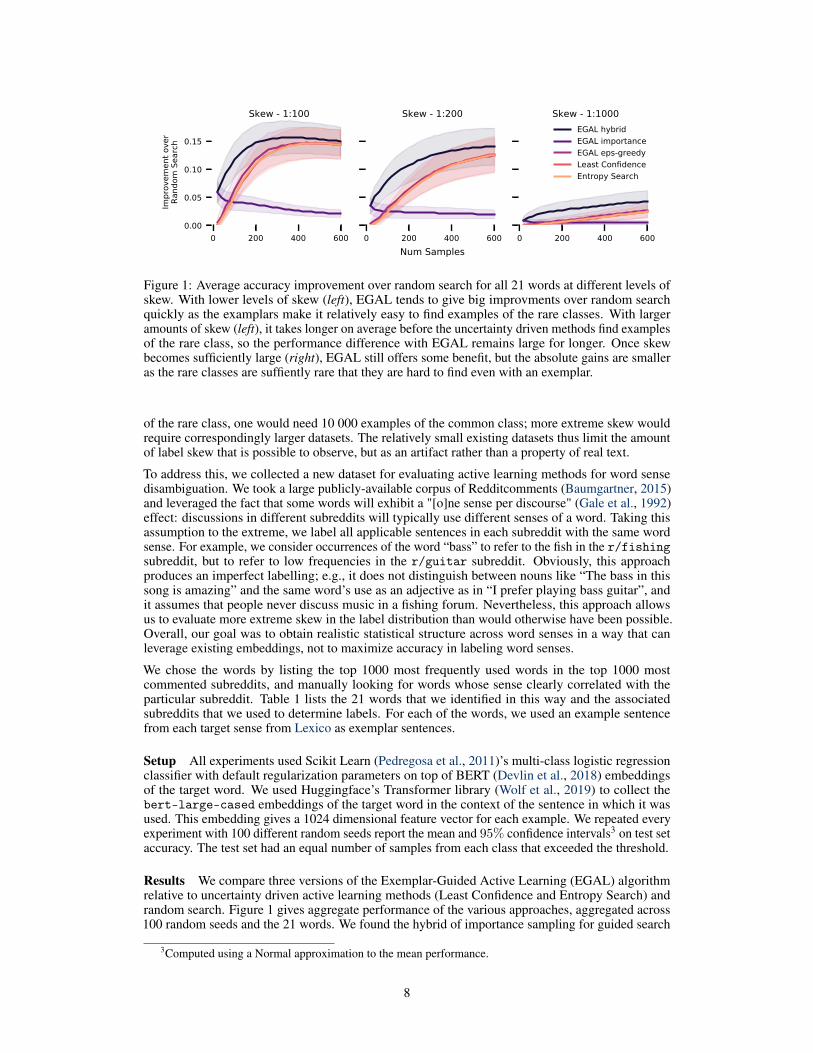
Figure 1: Average accuracy improvement over random search for all 21 words at different levels ofskew. With lower levels of skew (left), EGAL tends to give big improvments over random searchquickly as the examplars make it relatively easy to find examples of the rare classes. With largeramounts of skew (left), it takes longer on average before the uncertainty driven methods find examplesof the rare class, so the performance difference with EGAL remains large for longer. Once skewbecomes sufficiently large (right), EGAL still offers some benefit, but the absolute gains are smalleras the rare classes are suffiently rare that they are hard to find even with an exemplar.
of the rare class, one would need 10 000 examples of the common class; more extreme skew wouldrequire correspondingly larger datasets. The relatively small existing datasets thus limit the amountof label skew that is possible to observe, but as an artifact rather than a property of real text.
To address this, we collected a new dataset for evaluating active learning methods for word sensedisambiguation. We took a large publicly-available corpus of Redditcomments (Baumgartner, 2015)and leveraged the fact that some words will exhibit a "[o]ne sense per discourse" (Gale et al., 1992)effect: discussions in different subreddits will typically use different senses of a word. Taking thisassumption to the extreme, we label all applicable sentences in each subreddit with the same wordsense. For example, we consider occurrences of the word “bass” to refer to the fish in the r/fishingsubreddit, but to refer to low frequencies in the r/guitar subreddit. Obviously, this approachproduces an imperfect labelling; e.g., it does not distinguish between nouns like “The bass in thissong is amazing” and the same word’s use as an adjective as in “I prefer playing bass guitar”, andit assumes that people never discuss music in a fishing forum. Nevertheless, this approach allowsus to evaluate more extreme skew in the label distribution than would otherwise have been possible.Overall, our goal was to obtain realistic statistical structure across word senses in a way that canleverage existing embeddings, not to maximize accuracy in labeling word senses.
We chose the words by listing the top 1000 most frequently used words in the top 1000 mostcommented subreddits, and manually looking for words whose sense clearly correlated with theparticular subreddit. Table 1 lists the 21 words that we identified in this way and the associatedsubreddits that we used to determine labels. For each of the words, we used an example sentencefrom each target sense from Lexico as exemplar sentences.
Setup All experiments used Scikit Learn (Pedregosa et al., 2011)’s multi-class logistic regressionclassifier with default regularization parameters on top of BERT (Devlin et al., 2018) embeddingsof the target word. We used Huggingface’s Transformer library (Wolf et al., 2019) to collect thebert-large-cased embeddings of the target word in the context of the sentence in which it wasused. This embedding gives a 1024 dimensional feature vector for each example. We repeated everyexperiment with 100 different random seeds report the mean and 95% confidence intervals3 on test setaccuracy. The test set had an equal number of samples from each class that exceeded the threshold.
Results We compare three versions of the Exemplar-Guided Active Learning (EGAL) algorithmrelative to uncertainty driven active learning methods (Least Confidence and Entropy Search) andrandom search. Figure 1 gives aggregate performance of the various approaches, aggregated across100 random seeds and the 21 words. We found the hybrid of importance sampling for guided search
3Computed using a Normal approximation to the mean performance.
8

0 50 100 150 200 250 300
Num Samples
0.5
0.6
0.7
0.8
0.9
Acc
ura
cy
EGAL hybrid
EGAL importance
EGAL eps-greedy
Least Confidence
Guided Learner
Random Search
Entropy Search
0 50 100 150 200 250 300
Num Samples
0.5
0.6
0.7
0.8
0.9
1.0
Acc
ura
cy
EGAL hybrid
EGAL importance
EGAL eps-greedy
Least Confidence
Guided Learner
Random Search
Entropy Search
0 100 200 300 400 500 600
Num Samples
0.5
0.6
0.7
0.8
Acc
ura
cy
EGAL hybrid
EGAL importance
EGAL eps-greedy
Least Confidence
Guided Learner
Random Search
Entropy Search
Figure 2: Accuracy vs number of samples for bass (left), bank (middle) and fit (right), having labelskew of 1:60, 1:450 and 1:100 respectively. The word bass is a case where EGAL achieves significantgains with few samples; these gains are eventually evened out once the standard active learningmethods gain sufficient samples. Bank has both a high quality exemplar and extreme skew, leadingto large gains by using EGAL. Fit shows a failure case where EGAL’s performance does not differsignificantly from standard approaches.
and ✏-greedy active learning worked best across a variety of datasets. This EGAL hybrid approachoutperformed all baselines for all levels of skew, with the largest relative gains at 1:200: with 100examples labeled, EGAL had an increase in accuracy of 11% over random search and 5% over theactive learning approaches.
In Figure 2 we examine performance on three individual words and include guided learning as anoracle upper bound on the performance improve that could be achieved by a perfect exemplar searchroutine. On average guided learning achieved over 80� 90% accuracy on a balanced test for bothtasks using less than ten samples. By contrast, random search achieved 55% and 80% accuracy onbass and bank respectively, and did not perform better than random guessing on fit. This suggeststhat the key challenge for all of these datasets is collecting balanced examples. For the first two ofthese three datasets, having access to an exemplar sentence gave the EGAL algorithms a significantadvantage over the standard approaches; this difference was most stark on the bank dataset, whichexhibits far more extreme skew in the label distribution. On the fit dataset, EGAL did not significantlyimprove performance, but also did not hurt performance. These trends were typical (see the appendixfor all words): on two thirds of the words we tried, EGAL achieved significant improvements inaccuracy, while on the remaining third EGAL offered no significant improvements but also no cost ascompared to standard approaches. As with guided learning, direct comparisons between the methodsare not on equal footing: the exemplar classes give EGAL more information than the standardmethods have access to. However, we regard this as the key experimental point of our paper. EGALprovides a simple approach to getting potentially large improvements in performance when the labeldistribution is skewed, without sacrificing performance in settings where it fails to provide a benefit.
5 Conclusions
We present the Exemplar Guided Active Learning algorithm that leverages the embedding spaces oflarge scale language models to drastically improve active learning algorithms on skewed data. Wesupport the empirical results with theory that shows that the method is robust to mis-specified targetclasses and give practical guidance on its usage. Beyond word-sense disambiguation, we are nowusing EGAL to collect multi-word expression data, which shares the extreme skew property.
Broader Impact
This paper presents a method for better directing an annotation budget towards rare classes, withparticular application to problems in NLP. The result could be more money spent on annotationbecause such efforts are more worthwhile (increasing employment) or less money spent on annotationif “brute force” approaches become less necessary (reducing employment). We think the former ismore likely overall, but both are possible. Better annotation could lead to better language models,with uncertain social impact: machine reading and writing technologies can help language learnersand knowledge workers, increasing productivity, but can also fuel various negative trends includingmisinformation, bots impersonating humans on social networks, and plagiarism.
9

ReferencesAttenberg, J. and Ertekin, S. Class imbalance and active learning. 2013.
Attenberg, J. and Provost, F. Why label when you can search?: Alternatives to active learningfor applying human resources to build classification models under extreme class imbalance. InProceedings of the 16th ACM SIGKDD international conference on Knowledge discovery and data
mining, pp. 423–432. ACM, 2010.
Baumgartner, J. Complete Public Reddit Comments Corpus, 2015. URL https://archive.org/details/2015_reddit_comments_corpus.
Brent, R. Chapter 4: An Algorithm with Guaranteed Convergence for Finding a Zero of a Function.Prentice-Hall, 1973.
Chen, J., Schein, A., Ungar, L., and Palmer, M. An empirical study of the behavior of activelearning for word sense disambiguation. In Proceedings of the main conference on human
language technology conference of the north american chapter of the association of computational
linguistics, pp. 120–127. Association for Computational Linguistics, 2006.
Devlin, J., Chang, M.-W., Lee, K., and Toutanova, K. BERT: Pre-training of deep bidirectionaltransformers for language understanding. arXiv preprint arXiv:1810.04805, 2018.
Dligach, D. and Palmer, M. Good seed makes a good crop: Accelerating active learning usinglanguage modeling. In Proceedings of the 49th Annual Meeting of the Association for Computa-
tional Linguistics: Human Language Technologies, pp. 6–10, Portland, Oregon, USA, June 2011.Association for Computational Linguistics.
Edmonds, P. and Cotton, S. SENSEVAL-2: Overview. In Preiss, J. and Yarowsky, D. (eds.),SENSEVAL@ACL, pp. 1–5. Association for Computational Linguistics, 2001.
Fellbaum, C. WordNet: An Electronic Lexical Database. Bradford Books, 1998.
Gale, W. A., Church, K. W., and Yarowsky, D. One sense per discourse. In Proceedings of
the workshop on Speech and Natural Language, pp. 233–237. Association for ComputationalLinguistics, 1992.
Jiang, S., Garnett, R., and Moseley, B. Cost effective active search. In Wallach, H., Larochelle,H., Beygelzimer, A., d’Alché Buc, F., Fox, E., and Garnett, R. (eds.), Advances in Neural
Information Processing Systems 32, pp. 4880–4889. Curran Associates, Inc., 2019. URL http://papers.nips.cc/paper/8734-cost-effective-active-search.pdf.
Lattimore, T. and Szepesvári, C. Bandit Algorithms. Cambridge University Press, 2020.
Lexico. Lexico: Bass definition. https://www.lexico.com/en/definition/bass. Accessed: 2020-02-07.
Maurer, A. and Pontil, M. Empirical Bernstein bounds and sample variance penalization, 2009.
McCarthy, D., Koeling, R., Weeds, J., and Carroll, J. Unsupervised acquisition of predominant wordsenses. Computational Linguistics, 33(4):553–590, 2007.
Mihalcea, R., Chklovski, T., and Kilgarriff, A. The SENSEVAL-3 English lexical sample task. InProceedings of SENSEVAL-3: Third International Workshop on the Evaluation of Systems for the
Semantic Analysis of Text, pp. 25–28, 2004.
Pedregosa, F., Varoquaux, G., Gramfort, A., Michel, V., Thirion, B., Grisel, O., Blondel, M.,Prettenhofer, P., Weiss, R., Dubourg, V., Vanderplas, J., Passos, A., Cournapeau, D., Brucher, M.,Perrot, M., and Duchesnay, E. Scikit-learn: Machine learning in Python. Journal of Machine
Learning Research, 12:2825–2830, 2011.
Radford, A., Wu, J., Child, R., Luan, D., Amodei, D., and Sutskever, I. Language models areunsupervised multitask learners. 2019.
Raffel, C., Shazeer, N., Roberts, A., Lee, K., Narang, S., Matena, M., Zhou, Y., Li, W., and Liu, P. J.Exploring the limits of transfer learning with a unified text-to-text transformer. arXiv e-prints,2019.
10

Settles, B. Active learning, pp. 1–114. Morgan & Claypool Publishers, 2012.
Vaswani, A., Shazeer, N., Parmar, N., Uszkoreit, J., Jones, L., Gomez, A. N., Kaiser, Ł., andPolosukhin, I. Attention is all you need. In Advances in neural information processing systems, pp.5998–6008, 2017.
Virtanen, P., Gommers, R., Oliphant, T. E., Haberland, M., Reddy, T., Cournapeau, D., Burovski, E.,Peterson, P., Weckesser, W., Bright, J., van der Walt, S. J., Brett, M., Wilson, J., Jarrod Millman, K.,Mayorov, N., Nelson, A. R. J., Jones, E., Kern, R., Larson, E., Carey, C., Polat, I., Feng, Y., Moore,E. W., Vand erPlas, J., Laxalde, D., Perktold, J., Cimrman, R., Henriksen, I., Quintero, E. A.,Harris, C. R., Archibald, A. M., Ribeiro, A. H., Pedregosa, F., van Mulbregt, P., and Contributors,S. . . SciPy 1.0: Fundamental Algorithms for Scientific Computing in Python. Nature Methods,2020.
Wolf, T., Debut, L., Sanh, V., Chaumond, J., Delangue, C., Moi, A., Cistac, P., Rault, T., Louf,R., Funtowicz, M., and Brew, J. Huggingface’s transformers: State-of-the-art natural languageprocessing. ArXiv, abs/1910.03771, 2019.
Yuan, D., Richardson, J., Doherty, R., Evans, C., and Altendorf, E. Semi-supervised word sensedisambiguation with neural models. arXiv preprint arXiv:1603.07012, 2016.
Zhu, J. and Hovy, E. Active learning for word sense disambiguation with methods for addressing theclass imbalance problem. In Proceedings of the 2007 Joint Conference on Empirical Methods in
Natural Language Processing and Computational Natural Language Learning (EMNLP-CoNLL),pp. 783–790, Prague, Czech Republic, June 2007. Association for Computational Linguistics.
Zhu, J., Wang, H., Yao, T., and Tsou, B. K. Active learning with sampling by uncertainty and densityfor word sense disambiguation and text classification. In Proceedings of the 22nd International
Conference on Computational Linguistics (Coling 2008), pp. 1137–1144, Manchester, UK, August2008. Coling 2008 Organizing Committee.
11