Embed Size (px)
Citation preview

arX
iv:h
ep-p
h/02
0820
3v1
22
Aug
200
2
http://tumb1.biblio.tu-muenchen.de/publ/diss/ph/2002/bosch.html
MPI-PHT-2002-35June 2002
Exclusive Radiative Decays ofB Mesons in QCD Factorization
Stefan W. Bosch
Max-Planck-Institut fur Physik(Werner-Heisenberg-Institut)
Fohringer Ring 6D-80805 Munich, Germany
Email: [email protected]

Physik-DepartmentTechnische Universitat Munchen
Institut fur Theoretische PhysikLehrstuhl Univ.-Prof. A.J. Buras
Exclusive Radiative Decays ofB Mesons in QCD Factorization
Stefan W. Bosch
Vollstandiger Abdruck der von der Fakultat fur Physik der Technischen UniversitatMunchen zur Erlangung des akademischen Grades eines
Doktors der Naturwissenschaften (Dr. rer. nat.)
genehmigten Dissertation.
Vorsitzender: Univ.-Prof. Dr. Stephan Paul
Prufer der Dissertation: 1. Univ.-Prof. Dr. Andrzej J. Buras
2. Univ.-Prof. Dr. Gerhard Buchalla,Ludwig-Maximilians-Universitat Munchen
Die Dissertation wurde am 10. Juni 2002 bei der Technischen Universitat Munchen ein-gereicht und durch die Fakultat fur Physik am 22. Juli 2002 angenommen.


Abstract
We discuss exclusive radiative decays in QCD factorization within the Standard Model.In particular, we consider the decays B → V γ, with a vector meson K∗ or ρ in thefinal state, and the double radiative modes B0
s → γγ and B0d → γγ. At quark level,
all these decays are governed by the flavour-changing neutral-current b → sγ or b → dγtransitions, which appear at the one-loop level in the Standard Model. Such processesallow us to study CP violation and the interplay of strong and electroweak interactions, todetermine parameters of the CKM matrix, and to search for New Physics. The exclusivedecays are experimentally better accessible, but pose more problems for the theoreticalanalysis. The heavy-quark limit mb ≫ ΛQCD, however, allows to systematically separateperturbatively calculable hard scattering kernels from nonperturbative form factors anduniversal light-cone distribution amplitudes.
The main results of this work are the following:
• We apply QCD factorization methods based on the heavy-quark limit to thehadronic matrix elements of the exclusive radiative decays B → V γ and B → γγ.A power counting in ΛQCD/mb implies a hierarchy among the possible transitionmechanisms and allows to identify leading and subleading contributions. In partic-ular, effects from quark loops are calculable in terms of perturbative hard-scatteringfunctions and universal meson light-cone distribution amplitudes rather than beinggeneric, uncalculable long-distance contributions. Our approach is model indepen-dent and similar in spirit to the treatment of hadronic matrix elements in two-bodynon-leptonic B decays formulated by Beneke, Buchalla, Neubert, and Sachrajda.
• For the B → V γ decays we evaluate the leading ΛQCD/mb contributions completeto next-to-leading order in QCD. We adopt existing results for the hard-vertexcorrections and calculate in addition hard-spectator corrections, including also QCDpenguin operators.
• Weak annihilation topologies in B → V γ are shown to be power suppressed. Weprove to one-loop order that they are nevertheless calculable within QCD factor-ization. Because they are numerically enhanced we include the O(α0
s) annihilationcontributions of current-current and QCD-penguin operators in our analysis.
• The double radiative B → γγ decays are analyzed with leading-logarithmic accu-racy. In the heavy quark limit the dominant contribution at leading power comesfrom a single diagram. The contributions from one-particle irreducible diagramsare power suppressed but still calculable within QCD factorization. We use thesecorrections, including QCD penguins, to estimate CP asymmetries in B → γγ andso-called long-distance contributions in B and D → γγ.
• We predict branching ratios, CP and isospin asymmetries, and estimate U-spinbreaking effects for B → K∗γ and B → ργ. For the B → γγ decays we give numer-ical results for branching ratios and CP asymmetries. Varying the individual inputparameters we estimate the error of our predictions. The dominant uncertaintycomes from the poorly known nonperturbative input parameters.
i

ii
Contents
1 Introduction 1
I Fundamentals 5
2 The Basic Concepts 72.1 The Standard Model . . . . . . . . . . . . . . . . . . . . . . . . . . . . . . 72.2 Renormalization and Renormalization Group . . . . . . . . . . . . . . . . . 102.3 Operator Product Expansion . . . . . . . . . . . . . . . . . . . . . . . . . . 142.4 Effective Theories . . . . . . . . . . . . . . . . . . . . . . . . . . . . . . . . 162.5 The Effective b→ sγ Hamiltonian . . . . . . . . . . . . . . . . . . . . . . . 20
3 Factorization 253.1 Naive Factorization and its Offspring . . . . . . . . . . . . . . . . . . . . . 253.2 QCD Factorization . . . . . . . . . . . . . . . . . . . . . . . . . . . . . . . 27
3.2.1 The factorization formula . . . . . . . . . . . . . . . . . . . . . . . 273.2.2 The non-perturbative input . . . . . . . . . . . . . . . . . . . . . . 283.2.3 A simple application: Fγγπ0 . . . . . . . . . . . . . . . . . . . . . . 323.2.4 One-loop proof of factorization in B → Dπ . . . . . . . . . . . . . . 333.2.5 Limitations of QCD factorization . . . . . . . . . . . . . . . . . . . 37
3.3 Other Approaches to Non-Leptonic Decays . . . . . . . . . . . . . . . . . . 383.3.1 Dynamical approaches . . . . . . . . . . . . . . . . . . . . . . . . . 383.3.2 The diagrammatic way and flavour symmetry approaches . . . . . . 40
II The Radiative Decays B → V γ at NLO in QCD 43
4 Basic Formulas for B → V γ 454.1 What is the Problem? . . . . . . . . . . . . . . . . . . . . . . . . . . . . . 454.2 The Factorization Formula . . . . . . . . . . . . . . . . . . . . . . . . . . . 474.3 The Hard Vertex Corrections . . . . . . . . . . . . . . . . . . . . . . . . . 504.4 The Hard Spectator Corrections . . . . . . . . . . . . . . . . . . . . . . . . 544.5 The Annihilation Contribution . . . . . . . . . . . . . . . . . . . . . . . . . 574.6 A Comment on Power Corrections . . . . . . . . . . . . . . . . . . . . . . . 594.7 The Observables . . . . . . . . . . . . . . . . . . . . . . . . . . . . . . . . 60
iii

5 Phenomenology of B → V γ 635.1 Numerical results . . . . . . . . . . . . . . . . . . . . . . . . . . . . . . . . 635.2 Related Calculations . . . . . . . . . . . . . . . . . . . . . . . . . . . . . . 71
III The Radiative Decays B → γγ 73
6 The Basic Formulas for B → γγ 756.1 Motivation . . . . . . . . . . . . . . . . . . . . . . . . . . . . . . . . . . . . 756.2 Basic Formulas . . . . . . . . . . . . . . . . . . . . . . . . . . . . . . . . . 766.3 B → γγ at leading power . . . . . . . . . . . . . . . . . . . . . . . . . . . . 776.4 Power-suppressed contributions to B → γγ . . . . . . . . . . . . . . . . . . 786.5 Long-distance contributions to B and D → γγ . . . . . . . . . . . . . . . . 82
7 The Phenomenology of B → γγ 85
IV Conclusions 89
8 Conclusions 91
V Appendices 95
A Wilson Coefficients for b→ sγ 97
B Operator Basis Transformations 103
C Weak Annihilation in B → V γ 107
Bibliography 111
Acknowledgements 126
iv
Chapter 1
Introduction
Elementary particle physics represents man’s effort to answer the basic question: “Whatis the World Made of?” In search of the fundamental building blocks of matter physicistspenetrated to smaller and smaller constituents, which later turned out to be divisible. Theprimary matter of Anaximenes of Miletus, the periodic table of Mendeleev, Rutherford’salpha scattering experiments, the detection of the neutron by Chadwick and that of thepositron by Anderson, the discovery of nuclear fission by Hahn and Meitner, or Reinesfinding the neutrino were just some of the milestones on this way. What underlies ourcurrent theoretical understanding of nature is quantum field theory in combination with agauge principle. Electromagnetism, weak and strong nuclear forces, and their interactionwith quarks and leptons are described by the Standard Model of particle physics [1,2].Combined with general relativity, this theory is so far consistent with virtually all physicsdown to the scales probed by particle accelerators, roughly 10−16 cm, and also passes avariety of indirect tests that probe even shorter distances.
In spite of its impressive successes, the Standard Model is believed to be not com-plete. For a really final theory it is too arbitrary, especially considering the large numberof sometimes even “unnatural” parameters in the Lagrangian. Examples for such pa-rameters, that are largely different from what one naively expects them to be, are theweak scale compared with the Planck scale or the small value of the strong CP-violationparameter θQCD. Questions like: “Why are there three particle generations?”, “Why isthe gauge structure with the assignment of charges as it is?”, or “What is the origin of themass spectrum?” demand an answer by a really fundamental theory, but the StandardModel gives no replies. Furthermore, the union of gravity with quantum theory yields anonrenormalizable quantum field theory, indicating that New Physics should show up atvery high energies.
The ideas of grand unification, extra dimensions, or supersymmetry were put forwardto find a more complete theory. But applying these ideas has not yet led to theoriesthat are substantially simpler or less arbitrary than the Standard Model. To date, stringtheory [3], the relativistic quantum theory of one-dimensional objects, is a promising, andso far the only, candidate for such a “Theory of Everything”.
Within this thesis we work exclusively in the Standard Model, where particularlyin the flavour sector beside the aforementioned problems some unsolved issues remain.Among them are the mechanism of electroweak symmetry breaking and the hierarchyproblem that comes along with it, the generation of fermion masses, quark mixing, or
2 1. Introduction
the violation of the discrete symmetries C, P, CP, and T. Especially CP violation is ofparticular interest as it is one of the three vital ingredients to generate a cosmologicalmatter-antimatter asymmetry [4]. In 1964, James Cronin, Val Fitch, and collaboratorsdiscovered that the decays of neutral kaons do not respect CP symmetry [5]. Only recentlyCP violation was established undoubtfully also in the neutral B-meson system [6].
We will deal with the bottom quark system, which is an ideal laboratory for studyingflavour physics. The history of B physics started 1977 with the “observation of a dimuonresonance at 9.5GeV in 400GeV proton-nucleon collisions” at Fermilab [7]. It was bap-tized the “Υ resonance” and its quark content is bb. With the start of BaBar [8] and Belle[9] in 1999, dedicated B factories add a wealth of data to the results of CLEO [10] and theCERN [11] and Fermilab [12] experiments. The upcoming B-physics experiments at theTevatron Run II [13] and LHC [14] will bring us ever closer to the main goal of B physics,which is a precision study of the flavour sector with its phenomenon of CP violation topass the buck of being the experimentally least constrained part of the Standard Model.This is not only to pin down the parameters of the Standard Model, but in particularto reveal New Physics effects via deviations of measured observables from the StandardModel expectation. Such an indirect search for New Physics is complementary to thedirect search at particle accelerators. It invites both experimenters and theoreticians towork with precision. We need accurate and reliable measurements and calculations. Thecalculational challenge we will meet for this thesis are exclusive radiative decays of Bmesons.
But why investigate B meson decays? Due to confinement quarks appear in nature notseparately, but have to be bound into colourless hadrons. Considering constituent quarksonly, the simplest possible of such objects consists of a quark and an antiquark only andis called a meson. The bound states with a b quark and a d or u antiquark are referredto as the B0 and B− meson, respectively. Those B mesons containing an s or c quarkare denoted Bs and Bc, respectively. So “meson” decays because mesons are the simplesthadrons. But why of all mesons “B” mesons? Apart from the Υ resonances, the B mesonsare the heaviest mesons, because the top quark decays before it can hadronize. The factthat B mesons are heavy has two weighty consequences: B decays show an extremely richphenomenology and theoretical techniques using an expansion in the heavy mass allowfor model-independent predictions. The rich phenomenology is based on the one hand onthe large available phase space allowing for a plethora of possible final states and on theother hand on the possibility for large CP-violating asymmetries in B decays. The latterfeature is in contrast to the Standard Model expectations for decays of K and D mesons.In D decays only the comparably light d, s, and b quarks can enter internal loops whichleads to a strong GIM suppression of CP-violating phenomena. CP violation in K → ππis small due to flavour suppression and not because the CP violating phase itself is small.Actually, the sin 2β measurement in B → J/ψKS showed that the CP-violating phaseis large. Furthermore, especially the B → J/ψKS decay mode is theoretically extremelyclean as opposed to the large theoretical uncertainties in the kaon system. The patternof CP violation in the K and B system just represents the hierarchy of the CKM matrix.The B meson system offers an excellent laboratory to quantitatively test the CP-violatingsector of the Standard Model, determine fundamental parameters, study the interplay ofstrong and electroweak interactions, or search for New Physics.
We will concentrate on a subgroup of B decays: exclusive radiative B decays, i.e.
3
we are interested in the exclusive decay products of a B meson containing at least onephoton. The quark level decay is a flavour-changing-neutral-current process b → sγ orb → dγ. Such decays are rare, i.e. they come with small exclusive branching ratios ofO(10−5), because they arise only at the loop level in the Standard Model. Thereby theytest the detailed structure of the theory at the level of radiative corrections and provideinformation on the masses and couplings of the virtual SM or beyond-the-SM particlesparticipating. Among the rare B decays the b → sγ modes are the most prominent onesbecause they are already experimentally measured.
Primarily we are interested in the underlying decay of the heavy quark, which isgoverned by the weak interaction. But it is the strong force that is responsible for theformation of the hadrons that are observed in the detectors. If we want to do our exper-imental colleagues a favour, we let them measure the easier accessible exclusive decays,i.e. those where all decay products are detected. Then, however, we impose the burdenof a more difficult theoretical treatment on ourselves. The “easier” option for theorists isto consider the inclusive decay, where e.g. for B → Xsγ all final states with a photon andstrangeness content −1 have to be summed over. But quark-hadron duality allows us toconsider instead of all the B decays only the parton-level b→ sγ decay, which amounts toa fully perturbative calculation. Much effort was put into the inclusive mode to achieve afull calculation at next-to-leading order in renormalization-group-improved perturbationtheory. Yet, for the exclusive decays we have to dress the b quark with the “brown muck”,the light quark and gluon degrees of freedom inside the B meson, and have to keep strug-gling with hadronization effects. Despite the more complicated theoretical situation of theexclusive channels it is worthwhile to better understand them. Especially in the difficultenvironment of hadron machines, like the Fermilab Tevatron or the LHC at CERN, theyare easier to investigate experimentally. In any case the systematic uncertainties, bothexperimental and theoretical, are very different for inclusive and exclusive modes. A care-ful study of the exclusive modes can therefore yield valuable complementary informationin testing the Standard Model.
The field-theoretical tool kit at our disposal for this analysis includes operator productexpansion and renormalization group equations in the framework of an effective theory.Herewith the problem of calculating transition amplitudes can be separated into the per-turbatively calculable short distance Wilson coefficients and the long distance operatormatrix elements. In principle, the latter ones have to be calculated by means of a non-perturbative method like lattice QCD or QCD sum rules. For the exclusive decays of Bmesons, however, one can use additionally the fact that the b-quark mass mb is large com-pared to ΛQCD, the typical scale of QCD. This in turn allows one to establish factorizationformulas for the evaluation of the relevant hadronic matrix elements of local operatorsin the weak Hamiltonian. Herewith a further separation of long-distance contributionsto the process from a perturbatively calculable short-distance part, that depends onlyon the large scale mb, is achieved. The long-distance contributions have to be computednon-perturbatively or determined from experiment. However, they are much simpler instructure than the original matrix element. This QCD factorization technique was devel-oped by Beneke, Buchalla, Neubert, and Sachrajda for the non-leptonic two-body decaysof B mesons [15]. We apply similar arguments based on the heavy-quark limitmb ≫ ΛQCD
to the decays B → K∗γ, B → ργ, and B → γγ. This allows us to separate perturbativelycalculable contributions from the nonperturbative form factors and universal meson light-cone distribution amplitudes in a systematic way. With power counting in ΛQCD/mb we
4 1. Introduction
can identify leading and subleading contributions.
We have organized the subsequent 105 pages as follows: In the first part we fill ourtoolbox with the necessary ingredients. After a mini review of the Standard Model wepresent the basic equipment: operator product expansion, effective theories, and renor-malization group improved perturbation theory. A discussion of the effective b → sγHamiltonian and a short survey of its theoretical status quo concludes this chapter. Ourbest tool so far to treat the tough nut of exclusive B decays is QCD factorization. We de-vote Chapter 3 to the description of this useful technique. In order to be able to appreciateits merits we first present its predecessors “naive factorization” and generalizations. Wethen discuss rather in detail the QCD factorization approach, give a sample applicationto the calculation of the pion form factor, and mention limitations of QCD factorization.Finally, we comment on other attempts to treat hadronic matrix elements in exclusivenon-leptonic B decays.
Part II and III contain the main subject of this work: the treatment of B → V γ(V = K∗ or ρ) and B → γγ in QCD factorization. For both types of decays we firstpresent the necessary formulas and basic expressions and then give numerical results andphenomenological applications.
We derive for B → V γ the decay amplitude complete at next-to-leading order inQCD and leading power in ΛQCD/mb. Hard-vertex and hard-spectator corrections arediscussed separately. Annihilation contributions turn out to be power suppressed, butnevertheless calculable. As they are factorizable and numerically important we includethem for our phenomenological analysis. Doing so we become sensitive to the charge of thelight spectator quark inside the B meson and can estimate isospin breaking effects. Theseturn out to be large. The most important phenomenological quantity we predict is thebranching ratio. The NLL value is considerably larger than both the leading logarithmicprediction when the same form factor is used and the experimental value. Our calculationalso allows us to estimate CP-asymmetries and U-spin breaking effects. We want to stressthat this thesis is the first totally complete next-to-leading-logarithmic presentation ofexclusive B → V γ decays, and it is a model-indpendent one.
The double radiative B → γγ decays are analyzed with leading logarithmic accuracyin QCD factorization based on the heavy-quark limit mb ≫ ΛQCD. The dominant effectarises from the one-particle-irreducible magnetic-moment type transition b→ s(d)γ wherean additional photon is emitted from the light quark. The contributions from one-particleirreducible diagrams are power suppressed but still calculable within QCD factorization.They are used to compute the CP-asymmetry in B → γγ and to estimate so-called long-distance contributions in B and D → γγ. Numerical results are presented for branchingratios and CP asymmetries.
We give our conclusions and an outlook in chapter 8.Some more technical details are discussed in the Appendices. We give the explicit
formulas for the Wilson coefficients, transformation relations between the two operatorbases for b → sγ, and a one-loop proof that weak annihilation contributions to B → V γare calculable within QCD factorization.

Part I
Fundamentals


Chapter 2
The Basic Concepts
In this chapter we briefly introduce the basic concepts needed for doing calculations inelementary particle physics. We present the Standard Model in a nutshell and introducethe concepts of renormalization, renormalization group, operator product expansion, andeffective theories. We assume that the reader is familiar with quantum field and gaugetheories and refer to the pertinent textbooks [16].
2.1 The Standard Model
As mentioned already in the introduction, the Standard Model (SM) is a comprehensivetheory of particle interactions. Its success in giving a complete and correct description ofall non-gravitational physics tested so far is unprecedented. In the following we give a shortintroduction into this beautiful theory. We want to introduce the “Old Standard Model,”i.e. the one where neutrinos are massless. The recent evidence for neutrino masses,coming from the observation of neutrino oscillations [17], has no direct consequences forour work.
The Standard Model is made up of the Glashow-Salam-Weinberg Model [1] of elec-troweak interaction and Quantum Chromodynamics (QCD) [2]. It is based on the princi-ple of gauge symmetry. The Lagrangian of a gauge theory is invariant under local “gauge”transformations of a symmetry group. Such a symmetry can be used to generate dynamics- the gauge interactions. The prototype gauge theory is quantum electrodynamics (QED)with its Abelian U(1) local symmetry. It is believed that all fundamental interactions aredescribed by some form of gauge theory.
The gauge group of strong interactions is the non-Abelian group SU(3)C which haseight generators. These correspond to the gluons that communicate the strong force be-tween objects carrying colour charge - therefore the “C” as subscript. Since the gluonsthemselves are coloured, they can directly interact with each other, which leads to thephenomena of “asymptotic freedom” and “confinement.” At short distances, the couplingconstant αs becomes small. This allows us to compute colour interactions using per-turbative techniques and turns QCD into a quantitative calculational scheme. For longdistances on the other hand, the coupling gets large, which causes the quarks to be “con-fined” into colourless hadrons. In the words of Yuri Dokshitzer: “QCD, the marvelloustheory of the strong interactions, has a split personality. It embodies ‘hard’ and ‘soft’physics, both being hard subjects, the softer ones being the hardest.” [18]

8 2. The Basic Concepts
Electroweak interaction is based on the gauge group SU(2)L ⊗ U(1)Y - “L” standsfor “left” and “Y” denotes the hypercharge - which is spontaneously broken to U(1)QED.This is achieved through the non vanishing vacuum expectation value of a scalar isospindoublet Higgs field [19]
φ =
(φ+
φ0
)
(2.1)
Three of the four scalar degrees of freedom of the Higgs field give masses to the W and Zbosons. The remaining manifests itself in a massive neutral spin zero boson, the physicalHiggs boson. It is the only particle of the Standard Model which lacks direct experimentaldetection. The current lower limit on its mass is 114.1 GeV at the 95% confidence level[20]. From electroweak precision data there is much evidence for a light Higgs. But as soonas such a light Higgs is found, this gives birth to the hierarchy problem. A scalar (Higgs)mass is not protected by gauge or chiral symmetries so we expect mH ≈ Λ ≈ 1016GeV ifwe do not want to fine-tune the bare Higgs mass against the mass aquired from quantumeffects. Why should mH be much smaller than Λ?
Fermions are the building blocks of matter. In the SM they appear in three generationswhich differ only in their masses. The two species of fundamental fermions are leptons andquarks. With regard to the gauge group SU(2)L the quarks and leptons can be classedin left-handed doublets and right-handed singlets.
Quarks:
(ud ′
)
L
(cs ′
)
L
(tb′
)
L
uR cR tRdR sR bR
Leptons:
(νee−
)
L
(νµµ−
)
L
(νττ−
)
L
eR µR τR
Within the Old Standard Model there are no right-handed neutrinos. The quarks carrycolour charge and transform as SU(3)C triplets whereas the colourless leptons are SU(3)Csinglets.
Fermion masses are generated via a Yukawa interaction ψ(x)φ(x)ψ(x) with the Higgsfield (2.1). Using global unitary transformations in flavour space, the Yukawa interactioncan be diagonalized to obtain the physical mass eigenstates
d ′
s ′
b′
=
Vud Vus VubVcd Vcs VcbVtd Vts Vtb
︸ ︷︷ ︸
≡ VCKM
·
dsb
(2.2)
The non-diagonal elements of the Cabibbo-Kobayashi-Maskawa matrix [21] allow for tran-sitions between the quark generations in the charged quark current
J+µ =
(u, c, t
)
LγµVCKM
dsb
L
(2.3)

2.1 The Standard Model 9
b d
u,c,t u,c,t
d b
b s
u,c,t u,c,t
Figure 2.1: Example of a box and penguin diagram in the full theory. CP violating effects
are possible because quarks of all three generations are involved in the processes.
Unitarity of VCKM guaranties the absence of flavour-changing-neutral-current (FCNC)processes at tree level. This Glashow-Iliopoulos-Maiani (GIM) mechanism [22] wouldforbid FCNC transitions even beyond the tree level if we had exact horizontal flavoursymmetry which assures the equality of quark masses of a given charge. Such a symmetryis in nature obviously broken by the different quark masses so that at the one-loop leveleffective b→ s, b→ d, or s→ d processes like B → Xsγ or K → πνν can appear.
A unitary complex N × N matrix can be described by N2 real parameters. If thismatrix mixes N families each with two quarks one can remove 2N − 1 phases througha redefinition of the quark states, which leaves the Lagrangian invariant. Because anorthogonal N × N matrix has N(N − 1)/2 real parameters (angles) we are left withN2 − (2N − 1) − N(N − 1)/2 = (N − 1)(N − 2)/2 independent physical phases in thequark mixing matrix. Therefore, it is real if it mixes two generations only. The three-generation CKM matrix, however, has to be described by three angles and one complexphase. The latter one is the only source of CP violation within the Standard Model ifwe desist from the possibility that θQCD 6= 0. But these CP-violating effects can showup only if really all three generations of the Standard Model are involved in the process.Typically this is the case if one considers loop contributions of weak interaction, like boxor penguin diagrams as in Fig. 2.1.
In principle there are many different ways of parametrizing the CKM matrix. Forpractical purposes most useful is the so called Wolfenstein parametrization [23]
VCKM =
1− λ2
2λ Aλ3(ρ− iη)
−λ 1− λ2
2Aλ2
Aλ3(1− ρ− iη) −Aλ2 1
(2.4)
which is an expansion to O(λ3) in the small parameter λ = |Vus| ≈ 0.22. It is possible toimprove the Wolfenstein parametrization to include higher orders of λ [24]. In essence ρand η are replaced with ρ = ρ(1− λ2/2) and η = η(1− λ2/2), respectively.
For phenomenological studies of CP-violating effects, the so called standard unitaritytriangle (UT) plays a special role. It is a graphical representation of one of the six unitarityrelations, namely
VudV∗ub + VcdV
∗cb + VtdV
∗tb = 0 (2.5)
in the complex (ρ, η) plane. This unitarity relation involves simultaneously the elementsVub, Vcb, and Vtd which are under extensive discussion at present. The area of this andall other unitarity triangles equals half the absolute value of JCP = Im(VusVcbV
∗ubV
∗cs), the

10 2. The Basic Concepts
A = (ρ, η)
B = (1, 0)
1− ρ− iηρ+ iη
C = (0, 0)
γ
α
β
Figure 2.2: Unitarity Triangle
Jarlskog measure of CP violation [25]. Usually, one chooses a phase convention whereVcdV
∗cb is real and rescales the above equation with |VcdV ∗
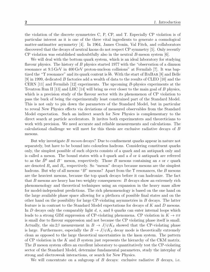
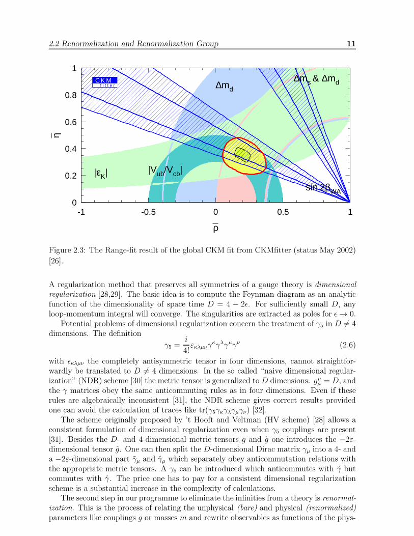
cb| = Aλ3. This leads to the trian-gle in Figure 2.2 with a base of unit length and the apex (ρ, η). A phase transformationin (2.5) only rotates the triangle, but leaves its form unchanged. Therefore, the anglesand sides of the unitarity triangle are physical observables and can be measured. Mucheffort was and is put into the determination of the UT parameters. One tries to measureas many parameters as possible. The consistency of the various measurements tests theconsequences of unitarity in the three generation Standard Model. Any discrepancy withthe SM expectations would imply the presence of new channels or particles contributingto the decay under consideration. So far, all experimental results are consistent with theStandard Model picture [26,27]. The state-of-the-art “frequentists” result for the unitar-ity triangle from the 2002 Winter conferences is displayed in Fig. 2.3 [26]. Actually thegood agreement of measurements with the Kobayashi-Maskawa mechanism gives rise tosome theoretical puzzles: the KM mechanism for example does explain neither the cosmicbaryon asymmetry nor the smallness of θQCD and basically all extensions of the StandardModel introduce a large number of new CP-violating phases.
2.2 Renormalization and Renormalization Group
Given the Lagrangian of a theory one can deduce the Feynman rules by means of whichamplitudes of the processes occuring in this theory can be calculated in perturbation the-ory. In Feynman diagrams with internal loops, however, one often encounters ultravioletdivergences. This is because the momentum variable of the virtual particle in the loopintegration ranges from zero to infinity. The theory of renormalization is a prescriptionwhich allows us to consistently isolate and remove all these infinities from the physicallymeasurable quantities. A two-step procedure is necessary.
First, one regulates the theory. That is, one modifies it in a way that observablequantities are finite and well defined to all orders in perturbation theory. We are then freeto manipulate formally these quantities, which are divergent only when the regularizationis removed. The most straightforward way to make the integrals finite is to introduce amomentum cutoff. But this violates for example Lorentz invariance or the Ward identities.
2.2 Renormalization and Renormalization Group 11
0
0.2
0.4
0.6
0.8
1
-1 -0.5 0 0.5 1
sin 2βWA
∆md
∆ms & ∆md
|εK| |Vub/Vcb|
ρ
η
C K Mf i t t e r
Figure 2.3: The Range-fit result of the global CKM fit from CKMfitter (status May 2002)
[26].
A regularization method that preserves all symmetries of a gauge theory is dimensionalregularization [28,29]. The basic idea is to compute the Feynman diagram as an analyticfunction of the dimensionality of space time D = 4 − 2ǫ. For sufficiently small D, anyloop-momentum integral will converge. The singularities are extracted as poles for ǫ→ 0.
Potential problems of dimensional regularization concern the treatment of γ5 in D 6= 4dimensions. The definition
γ5 =i
4!εκλµνγ
κγλγµγν (2.6)
with ǫκλµν the completely antisymmetric tensor in four dimensions, cannot straightfor-wardly be translated to D 6= 4 dimensions. In the so called “naive dimensional regular-ization” (NDR) scheme [30] the metric tensor is generalized toD dimensions: gµµ = D, andthe γ matrices obey the same anticommuting rules as in four dimensions. Even if theserules are algebraically inconsistent [31], the NDR scheme gives correct results providedone can avoid the calculation of traces like tr(γ5γκγλγµγν) [32].
The scheme originally proposed by ’t Hooft and Veltman (HV scheme) [28] allows aconsistent formulation of dimensional regularization even when γ5 couplings are present[31]. Besides the D- and 4-dimensional metric tensors g and g one introduces the −2ε-dimensional tensor g. One can then split the D-dimensional Dirac matrix γµ into a 4- anda −2ε-dimensional part γµ and γµ which separately obey anticommutation relations withthe appropriate metric tensors. A γ5 can be introduced which anticommutes with γ butcommutes with γ. The price one has to pay for a consistent dimensional regularizationscheme is a substantial increase in the complexity of calculations.
The second step in our programme to eliminate the infinities from a theory is renormal-ization. This is the process of relating the unphysical (bare) and physical (renormalized)parameters like couplings g or masses m and rewrite observables as functions of the phys-

12 2. The Basic Concepts
ical quantities. The renormalization procedure hides all divergences in a redefinition ofthe fields and parameters in the Lagrangian, i.e.
g0 = Zggµε m0 = Zmm
q0 = Z1/2q q Aµ
0 = Z1/23 Aµ (2.7)
and thus guaranties that measurable quantities stay finite. The index “0” indicates barequantities. Introducing the parameter µ with dimension of mass in (2.7) is necessary tokeep the coupling dimensionless. The factors Z are the renormalization constants. Therenormalization process is performed recursively in powers of the coupling constant g. Ifat every order of perturbation theory all divergences are reabsorbed in Z’s, the theory iscalled “renormalizable”. Theories with gauge symmetries, like the Standard Model, arerenormalizable. This is true even if the gauge symmetry is spontaneously broken via theHiggs mechanism because gauge invariance of the Lagrangian is conserved [33].
Renormalization can be straightforwardly implemented via the counter-term method.According to (2.7) the unrenormalized quantities are reexpressed through the renormalizedones in the original Lagrangian. Thus
L0 = L+ Lcounter (2.8)
The counter terms Lcounter are proportional to (Z−1) and can be treated as new interactionterms. For these new interactions Feynman rules can be derived and the renormalizationconstants Zi are determined such that the contributions from these new interactionscancel the divergences in the Green functions. This fixes the renormalization constantsonly up to an arbitrary subtraction of finite parts. Different finite parts define differentrenormalization schemes. In the Minimal Subtraction (MS) scheme only the divergencesand no finite parts are subtracted [34]. The modified MS scheme (MS) [35] defines thefinite parts such that terms ln 4π−γE , the artifacts of dimensional regularization, vanish.This can be achieved if one calculates with
µMS =µ eγE/2
√4π
(2.9)
instead of µ and performs minimal subtraction afterwards. We will exclusively work withthe MS scheme in the following.
Every renormalization procedure necessitates to introduce a dimensionful parameterµ into the theory. Even after renormalization the theoretical predictions depend on thisrenormalization scale µ. At this momentum scale the renormalization prescriptions, whichthe parameters of a renormalized field theory depend on, are applied. One “definesthe theory at the scale µ.” The bare parameters are µ-independent. To determine therenormalized parameters from experiment, a specific choice of µ is necessary: g ≡ g(µ),m ≡ m(µ), q ≡ q(µ). Different values of µ define different parameter sets g(µ), m(µ),q(µ). The set of all tranformations that relates parameter sets with different µ is calledrenormalization group (RG).
The scale dependence of the renormalized parameters can be obtained from the µ-independence of the bare ones. In QCD we get from (2.7) the renormalization groupequations (RGE) for the running coupling and the running mass
dg(µ)
d lnµ= β(g(µ), ε) (2.10)
dm(µ)
d lnµ= −γm (g(µ))m(µ) (2.11)

2.2 Renormalization and Renormalization Group 13
with the β-function
β(g(µ), ε) = −εg− 1
Zg
dZg
d lnµ︸ ︷︷ ︸
=: β(g)
(2.12)
and the anomalous dimension of the mass operator
γm (g(µ)) =1
Zm
dZm
d lnµ(2.13)
Calculating to two-loop accuracy we get
β(g) = − g3
16π2β0 −
g5
(16π2)2β1 (2.14)
γm(αs) =αs
4πγ(0)m +
(αs
4π
)2
γ(1)m (2.15)
where
β0 =11N − 2f
3β1 =
34
3N2 − 10
3Nf − 2CFf (2.16)
γ(0)m = 6CF γ(1)m = CF
(
3CF +97
3N − 10
3f
)
(2.17)
αs(µ) =g2(µ)
4πCF =
N2 − 1
2N(2.18)
with N the number of colours and f the number of active flavours. The solutions forαs(µ) and m(µ) then are [35]
αs(µ) =4π
β0 ln(µ2/Λ2MS
)
[
1− β1β20
ln ln(µ2/Λ2MS
)
ln(µ2/Λ2MS
)
]
(2.19)
m(µ) = m(µ0)
[αs(µ)
αs(µ0)
] γ(0)m2β0
[
1 +
(
γ(1)m
2β0− β1γ
(0)m
2β20
)
αs(µ)− αs(µ0)
4π
]
(2.20)
Here ΛMS is a characteristic scale both for QCD and the used MS scheme and depends
also on the number of effective flavours present in β0 and β1. An α(5)s (MZ) = 0.118±0.005
corresponds to Λ(5)
MS= 225+70
−57 MeV in NLO. It is interesting to note that such a massscale Λ emerges without making reference to any dimensional quantity and would bepresent also in a theory with completely massless particles. In QCD with three colours,even for six active flavours, both β0 = 7 and γ
(0)m /2β0 = 4/7 are positive. This leads
to asymptotic freedom as the coupling tends to zero with increasing µ. The pole atΛMS signals the breakdown of perturbation theory but gives a plausible argument forconfinement. Similarly, m(µ) decreases with µ getting larger.
A particularly useful application of the renormalization group is the summation oflarge logarithms. To see this we reexpress αs of (2.19) as
αs(µ) =αs(µ0)
v(µ)
[
1− β1β0
αs(µ0)
4π
ln v(µ)
v(µ)
]
(2.21)

14 2. The Basic Concepts
with
v(µ) = 1− β0αs
4πlnµ20
µ2(2.22)
If we expand the leading order term of (2.21) in αs(µ0) we get
αs(µ) = αs(µ0)∞∑
m=0
(
β0αs(µ0)
4πlnµ20
µ2
)m
(2.23)
Thus the solution of the RGE automatically sums the logarithms ln(µ20/µ
2) which getlarge for µ ≪ µ0. Generally, solving the RGE to order n sums in αs(µ) all terms of theform
αs(µ0)m+1
(
αs(µ0) lnµ20
µ2
)k
, 0 ≤ m ≤ n, k ∈ N0 (2.24)
This is particularly useful if, though αs(µ0) is smaller than one, the combinationαs(µ0) ln(µ
20/µ
2) is close to or even larger than one. Then the large logarithms wouldspoil the convergence of the perturbation series.
2.3 Operator Product Expansion
Up to now we treated processes of strong and electroweak interaction separately. Butall weak processes involving hadrons receive QCD corrections, which can be substantialespecially for non-leptonic and rare decays. The underlying quark level decay of a hadronis governed by the electroweak scale given by MW,Z = O(100GeV). On the other hand,the available energy inherent in a B meson decay is of O(mB). In dimensional regular-ization for example we encounter logarithms of the ratio of either of these scales with therenormalization scale µ. If the scales involved are widely separated it is not possible tomake all the logarithms small by a suitable choice of the renormalization scale. As wehave seen in the last section these large logarithms can be summed systematically usingrenormalization group techniques.
But we have yet another energy scale in the problem. A priori we cannot considerthe decay of free quarks. Due to confinement quarks appear in colourless bound systemsonly. The binding of the quarks inside the hadron via strong interaction is characterizedby a typical hadronic scale of O(1GeV). Here, even without large logarithms the strongcoupling αs is too large for perturbation theory to make sense. Unfortunately, in manycases the non-perturbative methods we have at hand nowadays are not yet developedenough to give accurate results.
Coming back to the typical energy mB in a B decay. Do we have to know at all what isreally going on at energies of O(100GeV) or the corresponding extremely short distances?In fact we do not. We also do not bother general relativity to calculate the trajectory ofan apple falling from a tree or QED and QCD to learn something about the propertiesof condensed matter. Instead, we employ Newtonian mechanics or the laws of chemistryand solid state physics, respectively. They are nonrelativistic approximations or effectivetheories appropriate for the low energy scale under consideration. This is exactly whatwe want to achieve for the weak interaction of quarks as well. The theoretical tool forthis purpose is operator product expansion (OPE) [36] which we shall introduce in thefollowing.

2.3 Operator Product Expansion 15
b c
u s
W
b c
u s
Figure 2.4: Replacing a W propagator with an effective four-fermion vertex.
For small separations, the product of two field operators A(x) and B(y) can be ex-panded in local operators Qi with potentially singular coefficient functions ci as
A(x)B(y) =∑
i
ci(x− y)Qi(x) (2.25)
The Wilson coefficient c1(z) accompanying the operator with lowest energy dimensionis the most singular one for z → 0 and the degree of divergence of the ci decreasesfor increasing operator dimension. Furthermore, for dimensional reasons, contributions ofoperators with higher dimension are suppressed by inverse powers of the heavy mass (smalldistance) scale. In principle, we have to consider all operators compatible with the globalsymmetries of the operator product AB. The physical picture is that a product of localoperators should appear as one local operator if their distance is small compared to thecharacteristic length of the system. One can systematically approximate the behaviour ofan operator product at short distances with a finite set of local operators. This is exactlywhat is done for the theory of weak decays.
Here, the mass of the W boson MW ≈ 80GeV is very large compared to a typicalhadronic scale. Therefore, the W propagator ∆µν(x, y) is of very short range only. Inthe amplitude of weak decays it connects two charged currents J−
µ (x) and J+ν (y), which
hence interact almost locally so that we can perform an OPE. Let us consider the quarklevel decay b→ csu for definiteness. The tree-level W -exchange amplitude for this decayis given by
A(b→ csu) = −GF√2VcbV
∗us
M2W
k2 −M2W
(su)V−A(cb)V−A
=GF√2VcbV
∗us (su)V−A(cb)V−A︸ ︷︷ ︸
local operator
+O(k2
M2W
)
(2.26)
Since the momentum transfer k through the W propagater is small as compared to MW ,we can safely neglect the terms O(k2/M2
W ). The W propagator then quasi shrinks to apoint (see fig. 2.4) and we obtain an effective four-fermion interaction. This is the modernformulation of the classical Fermi theory of weak interaction with GF = 1.166·10−5GeV−2
the Fermi constant. The Wilson coefficient in this example is simply one. The notation(q1q2)V−A in (2.26) is a practical shorthand for a left-handed charged quark current withthe chiral vector minus axialvector structure
(q1q2)V−A := q1γµ(1− γ5)q2 (2.27)
16 2. The Basic Concepts
2.4 Effective Theories
The result (2.26) can also be derived from an effective Hamiltonian
Heff =GF√2VcbV
∗us(su)V−A(cb)V−A + operators of higher dimension (2.28)
where the operators of higher dimensions correspond to the terms O(k2/M2W ) in (2.26)
and can likewise be neglected. In the effective theory the W boson is removed as anexplicit, dynamical degree of freedom. It is “integrated out” or “contracted out” usingthe language of the path integral or canonical operator formalism, respectively. One canproceed in a completely analougous way with the heavy quarks. This leads to effectivef quark theories where f denotes the “active” quarks, i.e. those that have not beenintegrated out.
If we include also short distance QCD or electroweak corrections more operators haveto be added to the effective Hamiltonian which we generalize to
Heff =GF√2
∑
i
V iCKMCi(µ)Qi(µ) (2.29)
Here the factor V iCKM denotes the CKM structure of the particular operator. If we want
to calculate the amplitude for the decay of a meson M = K, D, B, . . . into a final stateF we just have to project the Hamilton operator onto the external states
A(M → F ) = 〈F |Heff |M〉
=GF√2
∑
i
V iCKMCi(µ)〈F |Qi(µ)|M〉 . (2.30)
The Wilson coefficients Ci(µ) can be interpreted as the coupling constants for the effectiveinteraction terms Qi(µ). They are calculable functions of αs,MW , and the renormalizationscale µ. To any order in perturbation theory the Wilson coefficients can be obtained bymatching the full theory onto the effective one. This simply is the requirement that theamplitude in the effective theory should reproduce the corresponding amplitude in thefull theory. Hence, we first have to calculate the amplitude in the full theory and then thematrix elements 〈Qi〉. In this second step the resulting expressions may, even after quarkfield renormalization, be still divergent. Consequently we have to perform an operatorrenormalization
Q(0)i = ZijQj (2.31)
where Q(0)i denotes the unrenormalized operator. This notation is somewhat sloppy and
misleading. What actually is renormalized is not the operator but the operator matrixelements, or, even more exactly, the amputated Green functions 〈Qi〉. Then we have to
include the renormalization constant Z1/2q for each of the four external quark fields:
〈Qi〉(0) = Z−2q Zij〈Qj〉 (2.32)
In general, the renormalization constant Zij is a matrix so that operators carrying thesame quantum numbers can mix under renormalization. Operators of a given dimensionmix only into operators of the same or of lower dimension. Again, the divergent parts of

2.4 Effective Theories 17
the renormalization constant are determined from the requirement that the amplitude inthe effective theory is finite. The finite part in Zij on the other hand defines a specificrenormalization scheme. In a third step we extract the Wilson coefficients by comparingthe full and the effective theory amplitude. These are the Wilson coefficients at some fixedscale µ0. A caveat here is that the external states in the full and the effective theory haveto be treated in the same manner. Especially the same regularization and renormalizationschemes have to be used on both sides.
As the Wilson coefficients appear already at the level of the effective Hamiltonian,they are independent of the external states this Hamiltonian is projected onto to ob-tain the complete amplitude. When determining the Wilson coefficients, any external,even unphysical, state can be used. The coefficient functions represent the short-distancestructure of the theory. Because they depend for example on the masses of the par-ticles that were integrated out, they contain all information about the physics at thehigh energy scale. The long-distance contribution, on the other hand, is parametrizedby the process-dependent matrix elements of the local operators. This factorization ofSD and LD dynamics is one of the salient features of OPE. We can calculate the Wilsoncoefficients in perturbation theory and the hadronic matrix elements by means of somenon-perturbative technique like 1/N expansion, sum rules, or lattice gauge theory. Es-pecially to use the latter one, a separation of the SD part is essential for today’s latticesizes. The factorization can be visualized with large logarithms ln(M2
W/m2q) being split
into ln(M2W/µ
2) + ln(µ2/m2q). In doing so, the first logarithm will be retrieved in the
Wilson coefficients and the second one in the matrix elements. From this point of viewthe renormalization scale µ can be interpreted as the factorization scale at which the fullcontribution is separated into a low energy and a high energy part.
A typical scale at which to calculate the hadronic matrix elements of local operatorsis low compared to MW . For B decays we would choose µ = O(mB). Therefore, thelogarithm ln(M2
W/µ2) contained in the Wilson coefficient is large. So why not use the
powerful technique of summing large logarithms developped in section 2.2? In order todo so we have to find the renormalization group equations for the Wilson coefficientsand solve them. But so far the Wilson coefficients were not renormalized at all. Ifwe remember, however, that in the effective Hamiltonian the operators, which have to berenormalized, are accompanied always by the appropriate Wilson coefficent we can shufflethe renormalization as well to the Wilson coefficients. Let us start with the Hamiltonianof the effective theory with fields and coupling constants as bare quantities, which arerenormalized according to
q(0) = Z1/2q q (2.33)
C(0)i = Zc
ijCj (2.34)
Then the Hamiltonian (2.29) is in essence
Heff ∝ C(0)i Qi(q
(0))
≡ ZcijCjZ
2qQi
≡ CiQi + (Z2qZ
cij − δij)CjQi (2.35)
i.e. it can be written in terms of the renormalized couplings Ci and fields Qi plus countert-erms. The q(0) indicates that the interaction term Qi is composed of unrenormalized fields.
18 2. The Basic Concepts
If we calculate the amplitude with the Hamiltonian (2.35) including the counterterms, weget the finite renormalized result
Z2qZ
cijCj〈Qi〉(0) = Cj〈Qj〉 (2.36)
Comparing with (2.32) we read off the renormalization constant for the Wilson coefficients
Zcij = Z−1
ji (2.37)
So we can think of the operator renormalization in terms of the completely equivalentrenormalization of the coupling constants Ci, as in any field theory. If we again demandthe unrenormalized Wilson coefficients not to depend on µ we obtain the renormalizationgroup equation
dCi(µ)
d lnµ= γji(µ)Cj(µ) , (2.38)
with the anomalous dimension matrix for the operators
γij(µ) = Z−1ik
dZkj
d lnµ(2.39)
Let us simply state here that the numerical values for the γij can be determined directlyfrom the divergent parts of the renormalization constants Zij. In (2.38) the transposedof this anomalous dimension matrix appears. It is only the sign and the fact that theanomalous dimension is a matrix instead of a single number that distinguishes the RGEfor the Wilson coefficients from that of the running mass in (2.11). Therefore, we coulduse the solution (2.20) with the appropriate changes. To leading order this is in factpossible. But if we want to go to next-to-leading-order accuracy we run into problems,because the matrices γ
(0)ij and γ
(1)ij in the perturbative expansion
γij = γ(0)ij
αs
4π+ γ
(1)ij
(αs
4π
)2
+O(α3s) (2.40)
do not commute with each other. Let us instead formally write the solution for the Wilsoncoefficients with an evolution matrix U(µ, µ0)
Ci(µ) = Uij(µ, µ0)Cj(µ0) (2.41)
The leading order evolution matrix can be read off from (2.20)
U (0)(µ, µ0) =
[α(µ)
α(µ0)
]− γ(0)T
2β0
(2.42)
= V
[α(µ0)
α(µ)
]~γ(0)
2β0
D
V −1
where V is the matrix that diagonalizes γ(0)T
γ(0)D = V −1γ(0)TV (2.43)

2.4 Effective Theories 19
and ~γ(0) is the vector containing the eigenvalues of γ(0). For the next-to-leading ordersolution we make the clever ansatz
U(µ, µ0) =
[
1 +αs(µ)
4πJ
]
U (0)(µ, µ0)
[
1− αs(µ0)
4πJ
]
(2.44)
which proves to solve (2.38) if [37]
J = V HV −1 (2.45)
where the elements of H are
Hij = δijγ(0)i
β12β2
0
− Gij
2β0 + γ(0)i − γ
(0)j
(2.46)
withG = V −1γ(1)TV (2.47)
As we have mentioned in section 2.2, the procedure of renormalization allows to subtractarbitrary finite parts along with the ultraviolet singularities. Whereas physical quantitiesmust clearly be independent of the renormalization scheme chosen, at NLO unphysicalquantities, like the Wilson coefficients and the anomalous dimensions, depend on thechoice of the renormalization scheme. To ensure a proper cancellation of this schemedependence in the product of Wilson coefficients and matrix elements the same schemehas to be used for both. In order to uniquely define a renormalization scheme it is notsufficient to quote only the regularization and renormalization procedure but one also hasto choose a specific form for the so-called evanescent operators. These are operators whichexist in D 6= 4 dimensions but vanish in D = 4 [32,38,39].
So what do we have achieved so far? We have determined the Wilson coefficients ata scale µ0 via a matching procedure. These are the initial conditions for the evolutionfrom µ0 down to an appropriate low energy scale µ via U(µ, µ0) which sums large loga-rithms. Herefore, we had to determine the anomalous dimensions of the operators andsolve the renormalization group equation for the Wilson coefficients. We thus arrive at aRG improved perturbation theory and officially don’t speak any more of “leading” (LO)and “next-to-leading order” (NLO) but rather of “leading” (LL) and “next-to-leading-logarithmic order” (NLL). Yet, we might carelessly use the terms synonymously. In ourtask to evaluate weak decay amplitudes involving hadrons in the framwork of a low en-ergy effective theory we then only lack the calculation of the hadronic matrix elements〈Qi(µ)〉. This, however, is a highly non-trivial problem which this and many other worksare devoted to.
Looking at the complicated NLO formulas one might ask why at all going to next-to-leading order accuracy. After all these calculations imply the evaluation of two or evenmore loop diagrams which are technically very challenging. But they are very important.First of all we can test the validity of the renormalization group improved perturbationtheory. Then, of course, we hope that the theoretical uncertainties get reduced. Oneparticular issue is the residual renormalization scale dependence of the result. The scaleµ enters for example in αs(µ) or the running quark masses, in particular mt(µ), mb(µ),and mc(µ). In principle, a physical quantity cannot depend on the renormalization scale.But as we have to truncate the perturbative series at some fixed order, this property is

20 2. The Basic Concepts
broken. The renormalization scale dependence of Wilson coefficients and operator matrixelements cancels only to the order of perturbation theory included in the calculation.Therefore, one can use the remaining scale ambiguity as an estimate for the neglectedhigher order corrections. Usually one varies µ between half and twice the typical scaleof the problem, i.e. mb/2 < µ < 2mb for B decays. Going to NLO significantly reducesthese scale ambiguities. Furthermore, the renormalization scheme dependence of theWilson coefficients appears at NLO for the first time. Only if we properly match the longdistance matrix elements, obtained for example from lattice calculations, to the shortdistance contributions, these unphysical scheme dependences will cancel. Another issueis that the QCD scale ΛMS, which can be extracted from various high energy processes,cannot be used meaningfully in weak decays without going to NLO.
2.5 The Effective b→ sγ Hamiltonian
In this section we want to discuss the effective Hamiltonian necessary for the calculationsto follow. For b→ sγ transitions it reads
Heff =GF√2
∑
p=u,c
λ(s)p
[
C1Qp1 + C2Q
p2 +
∑
i=3,...,8
CiQi
]
(2.48)
whereλ(s)p = V ∗
psVpb (2.49)
The operators originate from the diagrams in Fig. 2.5 and are given by
Qp1 = (sp)V−A(pb)V−A (2.50)
Qp2 = (sipj)V−A(pjbi)V−A (2.51)
Q3 = (sb)V−A
∑
q
(qq)V−A (2.52)
Q4 = (sibj)V−A
∑
q
(qjqi)V−A (2.53)
Q5 = (sb)V−A
∑
q
(qq)V+A (2.54)
Q6 = (sibj)V−A
∑
q
(qjqi)V+A (2.55)
Q7 =e
8π2mb siσ
µν(1 + γ5)bi Fµν (2.56)
Q8 =gs8π2
mb siσµν(1 + γ5)T
aijbj G
aµν (2.57)
with e and gs the coupling constants of electromagnetic and strong interaction and Fµν
and Gµν the photonic and gluonic field strength tensors, respectively. In Q7 and Q8
we neglected the very small ms(1 − γ5) contribution. The i, j are colour indices. If nocolour index is given the two operators are assumed to be in a colour singlet state. Theoperator basis (2.50–2.57) consists of all possible gauge invariant operators with energydimension six with the following properties: they have the correct quantum numbers tocontribute to b→ sγ, they are compatible with the symmetries of electroweak interaction,
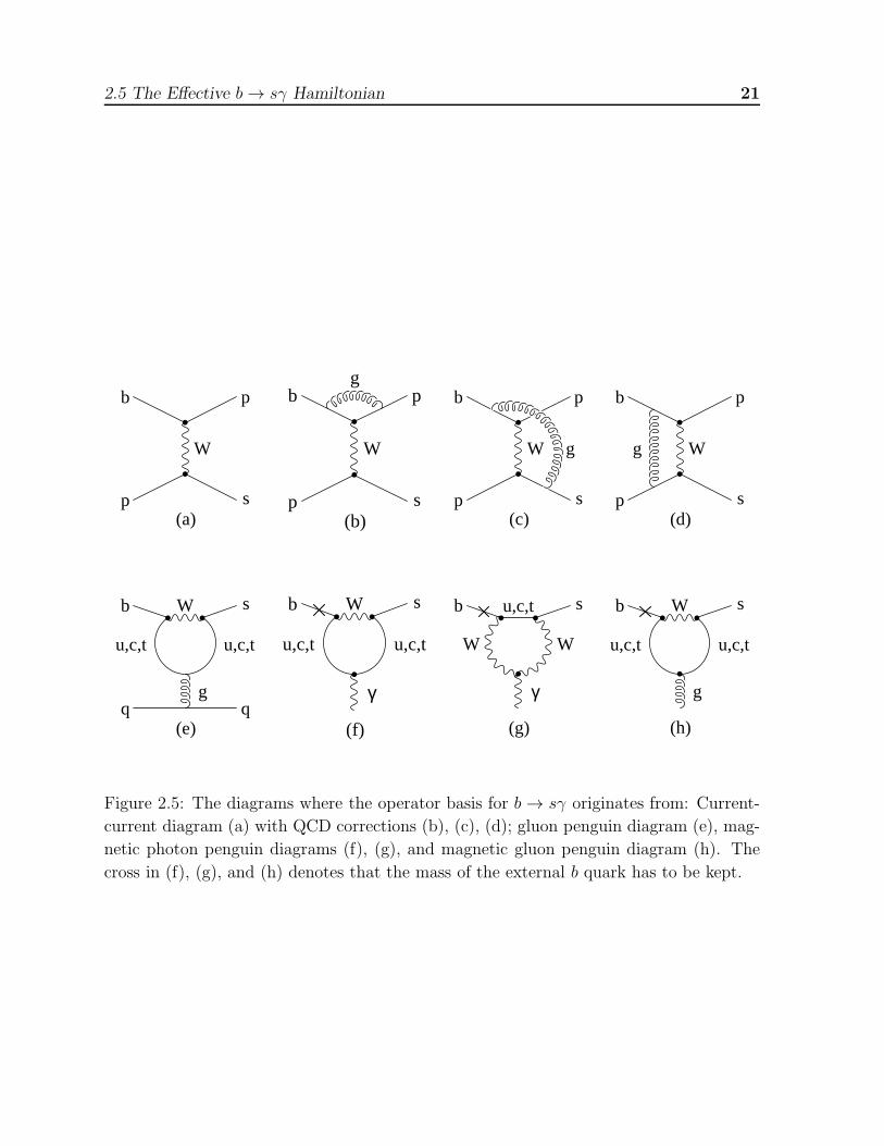
2.5 The Effective b→ sγ Hamiltonian 21
b p
p s
W
(a)
b p
p s
W
g
(b)
b p
p s
W g
(c)
b p
p s
Wg
(d)
b
s
u,c,t u,c,t
W
g
(e)
b s
u,c,t u,c,t
W
γ
(f)
b s
W W
u,c,t
γ
(g)
b s
u,c,t u,c,t
W
g
(h)
Figure 2.5: The diagrams where the operator basis for b → sγ originates from: Current-
current diagram (a) with QCD corrections (b), (c), (d); gluon penguin diagram (e), mag-
netic photon penguin diagrams (f), (g), and magnetic gluon penguin diagram (h). The
cross in (f), (g), and (h) denotes that the mass of the external b quark has to be kept.

22 2. The Basic Concepts
and they cannot be transformed into each other by applying equations of motion. As aconsequence, our operator basis is only the correct one if all external states are takenon-shell [40]. Additional operators have to be considered if an off-shell calculation isperformed. There is yet another operator basis used in the literature. It was introducedby Chetyrkin, Misiak, and Munz (CMM) [41,42] because then no Dirac traces containingγ5 arise in effective theory calculations, wich allows to use fully anticommuting γ5 indimensional regularization. It reads
P p1 = (sLγµT
apL)(pLγµT abL) (2.58)
P p2 = (sLγµpL)(pLγ
µbL) (2.59)
P3 = (sLγµbL)∑
q
(qγµq) (2.60)
P4 = (sLγµTabL)
∑
q
(qγµT aq) (2.61)
P5 = (sLγµ1γµ2γµ3bL)∑
q
(qγµ1γµ2γµ3q) (2.62)
P6 = (sLγµ1γµ2γµ3TabL)
∑
q
(qγµ1γµ2γµ3T aq) (2.63)
P7 =e
16π2mb(sLσ
µνbR)Fµν (2.64)
P8 =gs
16π2mb(sLσ
µνT abR)Gaµν (2.65)
where T a stand for SU(3)color generators and L = (1 − γ5)/2 and R = (1 + γ5)/2 forthe left and right-handed projection operators. We denote the corresponding Wilsoncoefficients with Zi. The operator basis (2.58–2.65) is in principle the more natural oneas the operators appear exactly in this form when calculating the diagrams of Fig. 2.5. Inour normal operator basis (2.50–2.57), the following four-dimensional identity was usedto “simplify” P5 and P6
γµγνγρ = gµνγρ + gνργµ − gµργν + iǫσµνργσγ5 in D = 4 (2.66)
This step, however, requires to introduce several more evanescent operators and leads toproblematic traces with γ5 in two-loop calculations. The choice of the operator’s colourstructure is more natural in the CMM basis, too, as it is the one emerging from thediagrams in Fig. 2.5.
In the common nomenclature Q1 and Q2 are called current-current operators, Q3...6
QCD penguin operators and Q7 and Q8 electromagnetic and chromomagnetic penguinoperator, respectively. For historical reasons the numbering of Qp
1,2 is sometimes reversedin the literature [43]. The sign conventions for the electromagnetic and strong couplingscorrespond to the covariant derivative Dµ = ∂µ + ieQfAµ + igT aAa
µ. The coefficients C7
and C8 then are negative in the Standard Model, which is the choice generally adoptedin the literature. The effective Hamiltonian for b→ dγ is obtained from equations (2.48–2.65) by the replacement s→ d.
Let us summarize the status quo in determining the effective Hamiltonian for b→ sγ.At leading order only Q7 contributes to b→ sγ. The corresponding Wilson coefficient wasfirst calculated by Inami and Lim in 1980 [44]. For the leading logarithmic RG improved
2.5 The Effective b→ sγ Hamiltonian 23
calculation the 8× 8 anomalous dimension matrix was obtained bit by bit. Mixing of thefour-quark operatorsQ1...6 among each other was considered already earlier for the analysisof nonleptonic decays [45]. The 2×2 submatrix for the magnetic penguins was obtained byGrinstein, Springer, and Wise [46]. Because the mixing of Q1...6 into Q7 and Q8 vanishesat the one-loop level, one has to perform two-loop calculations if the LL result for C7(µb)is wanted. This technical complication delayed the first completely correct result for the8× 8 anomalous dimension matrix until 1993 [47] followed by independent confirmations[48].
Going to next-to-leading order accuracy was highly desirable, because the leadinglogarithmic expression for the branching ratio B(B → Xsγ) suffers from sizable renor-malization scale uncertainties at the ±25% level. The step from leading order to leadinglogarithmic order already increased the branching ratio B(B → Xsγ) by almost a fac-tor of three [49–51]. The high-flying NLL enterprise was a joint effort of many groups.QCD corrections affect both Wilson coefficients and operator matrix elements. The O(αs)matching for the current-current operators was calculated already a long time ago [52], theone for the QCD penguins more than ten years later [53]. Two-loop matching is necessaryfor Q7 and Q8, which was achieved first by Adel and Yao [54] and subsequently checkedthoroughly [55,56]. The O(α2
s) contributions to the 6 × 6 anomalous dimension matrixwere calculated in [32,52,53,57], the submatrix for Q7 and Q8 in [58]. Chetyrkin, Misiak,and Munz finally succeeded in determining the three-loop mixing of four-quark operatorsinto magnetic penguin operators [41]. The explicit formulas for the Wilson coefficientsneeded subsequently can be found in Appendix A, and in Appendix B we comment onthe transformation properties of the two operator bases used in this work.
For the inclusive decay B → Xsγ, i.e. the radiative decay of a B meson into the sumof final states with strangeness S = −1, the operator matrix elements can be computedperturbatively employing the heavy-quark expansion (HQE) [59]. This method consistsof an OPE in inverse powers of the large dynamical scale of energy release ∼ mb followedby a nonrelativistic expansion for the b field. Using the optical theorem, the inclusiveB-decay rate can be written in terms of the absorptive part of the forward scatteringamplitude 〈B|T |B〉. The transition operator T is the absorptive part of the time-orderedproduct of Heff(x)Heff(0)
T = Im
[
i
∫
d4xTHeff(x)Heff(0)
]
(2.67)
If we insert a complete set of states inside the time-ordered product we see that this wasjust a fancy way of writing the standard expression for the decay rate
Γ(B → X) =1
2mB
∑
X
(2π)4δ4(pB − pX) |〈X|Heff |B〉|2 (2.68)
However, the formulation in terms of the T product allows for a direct evaluation usingFeynman diagrams. Because of the large mass of the b quark, we can construct an OPE inwhich T is represented as a series of local operators containing the heavy-quark fields. Theoperator of lowest dimension is bb. Its matrix element is simplified by a nonrelativisticexpansion in powers of 1/mb starting with unity. In the limit of an infinitely heavy bquark the B meson decay rate is therefore given by the b quark decay rate. This quark-hadron duality is of great use for many inclusive calculations and justifies for example

24 2. The Basic Concepts
the spectator model. Corrections to this relation appear only at O(1/m2b) because the
potential dimension 4 operator bD/ b can be reduced to mbbb. However, the OPE onlyconverges for sufficiently inclusive observables. But for B → Xsγ decays experimentalcuts are necessary to reduce the background from charm production. This restricts theavailable phase space considerably leading to complications of the OPE based analysis.
The virtual corrections to the matrix elements 〈sγ|Q1,7,8|b〉 were first calculated byGreub, Hurth, and Wyler [60] and checked by Buras, Czarnecki, Misiak, and Urban usinganother method [61]. The latter authors presented recently also the last missing itemin the NLO analysis of B → Xsγ, namely the two-loop matrix elements of the QCD-penguin operators [62]. Yet, their contribution is numerically very small because thecorresponding Wilson coefficients almost vanish. The Bremsstrahlung corrections, i.e.the process b → sγg, influence especially the photon energy spectrum. At leading orderthis spectrum is a δ function, smeared out by the Fermi motion of the b quark inside theB meson, whereas it is broadened substantially at NLO [63].
Even higher electroweak corrections have been calculated for B → Xsγ [64]. Finally,there are non-perturbative contributions which can be singled out in the framework ofHQE. The 1/m2
b corrections mainly account for the fact that in reality a B meson andnot a b quark is decaying. Additionally, one has to consider long distance contributionsoriginating in the photon coupling to a virtual cc loop. This Voloshin effect is proportionalto 1/m2
c and enhances the decay rate by 3% [65–67].All this effort was taken to reduce the theoretical error and account for the ever in-
creasing experimental precision. The current experimental world average for the inclusivebranching fraction is
B(B → Xsγ)exp = (3.23± 0.42) · 10−4 (2.69)
combining the results of [68–70]. For the theoretical prediction [62]
B(B → Xsγ)thEγ>1.6GeV = (3.57± 0.30) · 10−4 (2.70)
there is an ongoing discussion about quark mass effects. The matrix elements of Q1
depend at two-loop level on the mass ratio m2c/m
2b . Gambino and Misiak [71] argue that
the running charm quark mass should be used instead of the pole mass, because the charmquarks in the loop are dominantly off-shell. Strictly speaking, this is a NNLO issue andcould be used to estimate the sensitivity to NNLO corrections. Numerically, however, itincreased the branching ratio by 11%. A more conservative error estimate would ratheradd this shift to the theoretical error.
As b → sγ decays appear at one-loop level for the first time, they play an impor-tant role in indirect searches for physics beyond the Standard Model. Effects from newparticles in the loops could easily be of the same order of magnitude than the StandardModel contributions. The excellent agreement of experimental measurement (2.69) andtheoretical prediction (2.70) therefore places severe bounds on the parameter space ofNew Physics scenarios, like multi-Higgs models [56,72], Technicolor [73], or the MSSM[74].
The treatment of the matrix elements for exclusive b→ sγ decays as for example B →K∗γ is in general more complicated. In this case, bound-state effects are essential andneed to be described by non-perturbative hadronic quantities like form factors. Exactlythese exclusive radiative decays of B mesons are the subject of this work and will be dealtwith in detail in part II and III.

Chapter 3
Factorization
The idea of factorization in hadronic decays of heavy mesons is already quite old. Let us inthe following sections describe “naive factorization” and its extensions, state the problemsand shortcomings of these models, and then introduce QCD factorization, which allowsfor a systematic and model-independent treatment of two-body B decays. In the lastsection of this chapter we will shortly present some other approaches used to tackle thedifficulties with these decays.
3.1 Naive Factorization and its Offspring
For leptonic and semi-leptonic two-body decays, the amplitude can be factorized into theproduct of a leptonic current and the matrix element of a quark current, because gluonscannot connect quark and lepton currents. Pictorially spoken, the Feynman diagram fallsapart into two simpler separate diagrams if we cut the W propagator. For non-leptonicdecays, however, we also have non-factorizable contributions, because gluons can connectthe two quark currents and additional diagrams can contribute.
In highly energetic two-body decays, hadronization of the decay products takes placenot until they have separated already. If the quarks have arranged themselves intocolour-singlet pairs, low-energetic (soft) gluons cannot affect this arrangement (colourtransparency) [75,76]. In the naive factorization approach, the matrix element of a four-fermion operator in a heavy-quark decay is assumed to separate (“factorize”) into twofactors of matrix elements of bilinear currents with colour-singlet structure [77,78], e.g.
〈D+π−|(cb)(V−A)(du)(V−A)|Bd〉 → 〈π−|(du)(V−A)|0〉〈D+|(cb)(V −A)|Bd〉∝ fπF
B→D (3.1)
In general, the complicated non-leptonic matrix elements 〈M1M2|Qi|B〉 are decomposedinto a form factor FB→M1 and a meson decay constant fM2. The factorized matrix elementsof Q1 and Q2 are dressed with the parameters
a1,2 = C1,2(µ) +C2,1(µ)
N(3.2)
respectively, to give the amplitude. In the literature one distinguishes three classes of non-leptonic two-body decays. The first class contains only a1 such that the meson generated

26 3. Factorization
from the colour-singlet current is charged as in (3.1). The second class involves only a2and therefore consists of those decays in which the meson generated directly from thecurrent is neutral. The third class finally covers decays in which the a1 and a2 amplitudesinterfere.
Already two of the prominent proponents of factorization in heavy meson decays,Dugan and Grinstein, admitted that “at first sight, factorization is a ridiculous idea.”[76]. In (3.1) the exchange of “non-factorizable”1 gluons between the π− and the (BdD
+)system was completely neglected, which consequently does not allow for rescattering inthe final state and for the generation of a strong phase shift between different amplitudes.Yet, the main problem of naive factorization is that it reduces the renormalization scaledependent matrix element to the form factor and decay constant, which have a ratherdifferent scale dependence. This destroys the cancellation of the scale dependence inthe amplitude and is therefore unphysical. Naive factorization cannot be correct exactlyand gives at most an approximation for one single suitable factorization scale µf . Thevalue of this particular scale is not provided by the model itself, but usually expectedto be O(mb) and O(mc) for B and D decays, respectively. Another problem with naivefactorization arises beyond the leading logarithmic level. Here, the Wilson coefficientsbecome renormalization scheme dependent whereas the factorized matrix elements arerenormalization scheme independent such that no cancellation of the scheme dependencein the amplitude can take place. This is unphysical again.
The concept of “generalized factorization” tries to solve these problems by introducingnon-perturbative hadronic parameters, which shall quantify the “non-factorizable” con-tributions and herewith cancel the scale and scheme dependence of the Wilson coefficients[79–81]. Neubert and Stech [80] replace a1 and a2 by
aeff1 =
(
C1(µ) +C2(µ)
N
)
[1 + ε(BD,π)1 (µ)] + C2(µ)ε
(BD,π)8 (µ)
aeff2 =
(
C2(µ) +C1(µ)
N
)
[1 + ε(Bπ,D)1 (µ)] + C1(µ)ε
(Bπ,D)8 (µ) (3.3)
Due to the aforementioned renormalization scheme dependence, however, it is possibleto find for any chosen scale µf a renormalization scheme in which the non-perturbativeparameters ε1(µf) and ε8(µf) vanish simultaneously [82]. This leads back to naive factor-ization instead of describing the “non-factorizable” contributions to non-leptonic decaysproperly. Another variant of generalized factorization achieves the scale and scheme in-dependence via effective Wilson coefficient functions and an effective number of colours[81]:
aeff1,2 = Ceff1,2 +
1
N effCeff
2,1 (3.4)
Again, these effective parameters are nicely renormalization scale and scheme indepen-dent. Yet, Buras and Silvestrini [82] showed that they depend on the gauge and theinfrared regulator and are thus unphysical.
All these shortcomings are resolved in the QCD factorization approach.
1We put quotes on “non-factorizable” if we mean the corrections to naive factorization to avoid
confusion with the meaning of factorization in the context of hard processes in QCD.
3.2 QCD Factorization 27
3.2 QCD Factorization
The typical scale for a B meson decay is of order mB and therefore much larger thanΛQCD, the long-distance scale where non-perturbative QCD takes over. QCD factoriza-tion, introduced by Beneke, Buchalla, Neubert, and Sachrajda, uses exactly this fact [15].This time, something is factorized in the general sense of QCD applications: Namelythe long-distance dynamics in the matrix elements and the short-distance interactionsthat depend only on the large scale mB. And again, the short-distance contributionscan be computed in a perturbative expansion in the strong coupling αs (O(mb)). Thelong-distance part has still to be computed non-perturbatively or determined experimen-tally. However, these non-perturbative parameters are mostly simpler in structure thanthe original matrix element and they are process independent.
3.2.1 The factorization formula
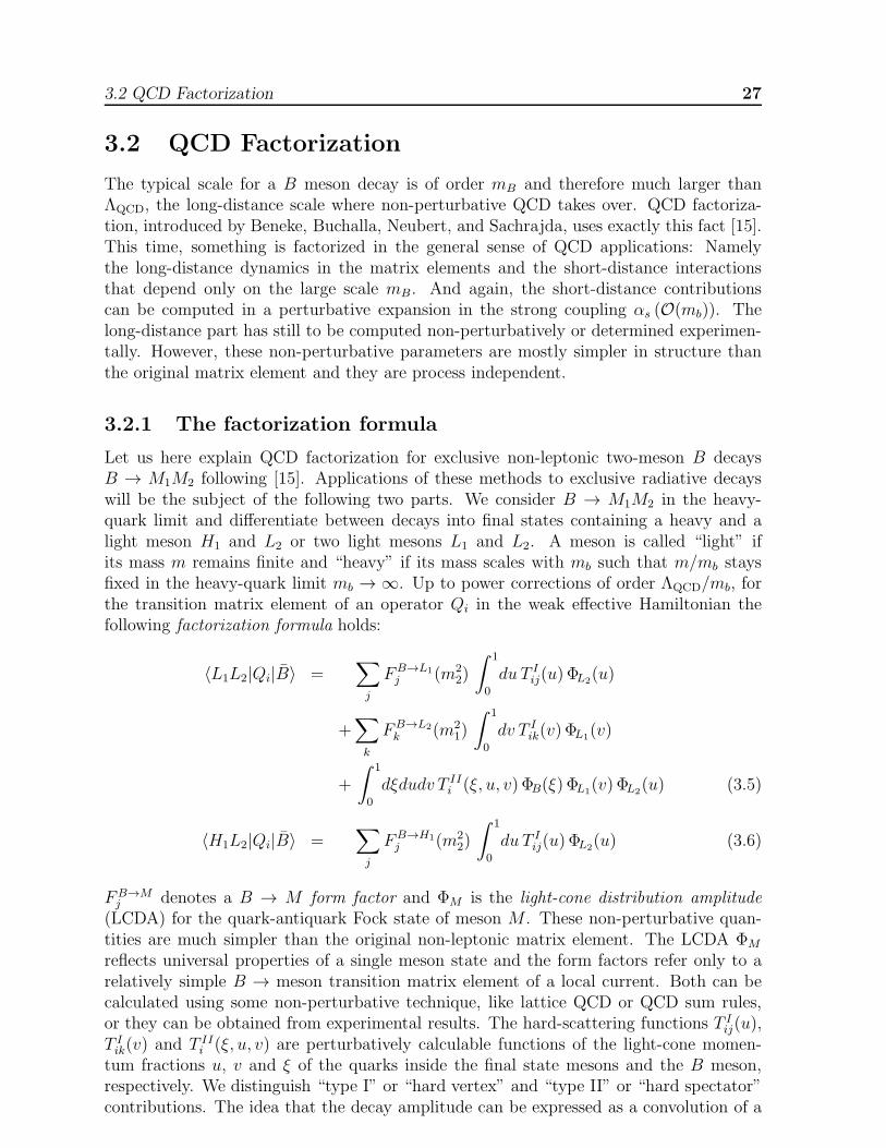
Let us here explain QCD factorization for exclusive non-leptonic two-meson B decaysB → M1M2 following [15]. Applications of these methods to exclusive radiative decayswill be the subject of the following two parts. We consider B → M1M2 in the heavy-quark limit and differentiate between decays into final states containing a heavy and alight meson H1 and L2 or two light mesons L1 and L2. A meson is called “light” ifits mass m remains finite and “heavy” if its mass scales with mb such that m/mb staysfixed in the heavy-quark limit mb → ∞. Up to power corrections of order ΛQCD/mb, forthe transition matrix element of an operator Qi in the weak effective Hamiltonian thefollowing factorization formula holds:
〈L1L2|Qi|B〉 =∑
j
FB→L1j (m2
2)
∫ 1
0
du T Iij(u) ΦL2(u)
+∑
k
FB→L2
k (m21)
∫ 1
0
dv T Iik(v) ΦL1(v)
+
∫ 1
0
dξdudv T IIi (ξ, u, v) ΦB(ξ) ΦL1(v) ΦL2(u) (3.5)
〈H1L2|Qi|B〉 =∑
j
FB→H1j (m2
2)
∫ 1
0
du T Iij(u) ΦL2(u) (3.6)
FB→Mj denotes a B → M form factor and ΦM is the light-cone distribution amplitude
(LCDA) for the quark-antiquark Fock state of meson M . These non-perturbative quan-tities are much simpler than the original non-leptonic matrix element. The LCDA ΦM
reflects universal properties of a single meson state and the form factors refer only to arelatively simple B → meson transition matrix element of a local current. Both can becalculated using some non-perturbative technique, like lattice QCD or QCD sum rules,or they can be obtained from experimental results. The hard-scattering functions T I
ij(u),T Iik(v) and T II
i (ξ, u, v) are perturbatively calculable functions of the light-cone momen-tum fractions u, v and ξ of the quarks inside the final state mesons and the B meson,respectively. We distinguish “type I” or “hard vertex” and “type II” or “hard spectator”contributions. The idea that the decay amplitude can be expressed as a convolution of a

28 3. Factorization
L1
L2
ΦL1
T Iik
FM2k
B+
L1
L2
ΦL2
T Iij
B
FM1j
T IIi
ΦL2
ΦL1
ΦBB
L2
L1
+
Figure 3.1: Graphical representation of the factorization formula for a B meson decaying
into two light mesons, e.g. B− → π0K−. At leading order in ΛQCD/mb there are no
long-distance interactions between the system of B meson and the meson that picks up
the spectator quark, and the other final state meson.
hard-scattering factor with light-cone wave functions of the participating mesons is anal-ogous to more familiar applications of this method to hard exclusive reactions involvingonly light hadrons [83]. A graphical representation of (3.5) is given in Fig. 3.1.
When the spectator quark in the B meson goes to a heavy meson as in Bd → D+π−,the spectator interaction is power suppressed in the heavy-quark limit and we arrive atthe simpler equation (3.6). For the opposite situation where the spectator quark goes to alight meson, but the other meson is heavy, factorization does not hold, because the heavymeson is neither fast nor small and cannot be factorized from the B → M1 transition.Annihilation topologies do not contribute at leading order in the heavy-quark expansion.
The hard spectator interactions appear at O(αs) for the first time. Since at O(α0s)
the functions T Iij/k are independent of u and v, the convolution integral results in a meson
decay constant and we see that (3.5) and (3.6) reproduce naive factorization. We now,however, can systematically compute radiative corrections to naive factorization. Thisimmediately solves the problem of scale and scheme dependence in the conventional fac-torization approaches. Because the form factors are real quantities, all strong rescatteringphases are either generated perturbatively or are power suppressed.
In principle, QCD factorization is nothing else but a consistent formalization andgeneralization of Bjorken’s colour transparency argument [75]. This is most obvious forthe decay Bd → D+π−. The spectator quark and the other light degrees of freedominside the B meson can easily form a D meson after the weak b→ c decay. This B → Dtransition can be parametrized by a set of form factors. The other two light quarks arevery energetic. To form a pion they must be highly collinear and in a colour-singletconfiguration, the probability of which is described by the leading-twist pion light-conedistribution amplitude. Such an energetic “colour-transparent” compact object can leavethe decay region without interfering with the D meson formation because soft interactionsdecouple.
3.2.2 The non-perturbative input
We will now discuss the necessary non-perturbative input, namely form-factors and light-cone distribution amplitudes, in more detail.

3.2 QCD Factorization 29
Form factors
A form factor is a function of scalar variables accompanying the independent terms in themost general decomposition of the matrix element of a current consistent with Lorentzand gauge invariance. In the literal meaning a form factor goes with the matrix elementof some current where initial and final state are one and the same particle. In the non-relativistic limit a particle has two electromagnetic form factors, which are simply theFourier transforms of its charge and magnetic moment distributions. They thereforeindeed give information on the form of the particle under consideration.
In the context of QCD factorization we often need the matrix element of the vectorcurrent which is conventionally parametrized by two scalar form factors
〈P (k)|qγµb|B(p)〉 = FB→P+ (q2) (pµ + kµ) +
[
FB→P0 (q2)− FB→P
+ (q2)] m2
B −m2P
q2qµ (3.7)
where q = p−k. Strictly speaking FB→P0/+ are transition form factors, which do not describe
the form of neither the B meson nor the pseudoscalar meson P , but rather their overlapduring the weak decay. For q2 = 0 the two form factors coincide, FB→P
+ (0) = FB→P0 (0).
The scaling behaviour of the form factors is
FB→D0/+ (0) ∼ 1 (3.8)
FB→π0/+; hard(0) ∼ αs
(√
mbΛQCD
)(ΛQCD
mb
)3/2
(3.9)
FB→π0/+; soft(0) ∼
(ΛQCD
mb
)3/2
(3.10)
for the B → D and B → π transition, respectively [15,84]. Both the heavy-to-heavyand heavy-to-light B → M form factors receive a leading contribution from soft gluonexchange. This is why the form factor has to enter the factorization formula as a non-perturbative input.
Light-cone distribution amplitudes for light mesons
Let us now consider the other non-perturbative ingredients which are the meson light-conedistribution amplitudes. We define light-cone components
k± =k0 ± k3√
2(3.11)
for any four vector kµ = (k+, k−, ~k⊥). These variables naturally distinguish betweena particle’s longitudinal and transverse degrees of freedom. Let us construct a lightpseudoscalar meson out of the on-shell constituent quarks in a spin singlet state and withno net transverse momentum:
|P (k)〉 =∫
dv√vv
d2l⊥16π3
1√2
(
a†l1↑b†l2↓
− a†l1↓b†l2↑
)
|0〉ψ(v, l⊥) (3.12)
where a†l↑ (b†l↑) creates a (anti)quark with momentum l and spin up. Their momentum
shall be a fraction v and v of the meson momentum k: l+1 = vk+ and l+2 = vk+ plus a
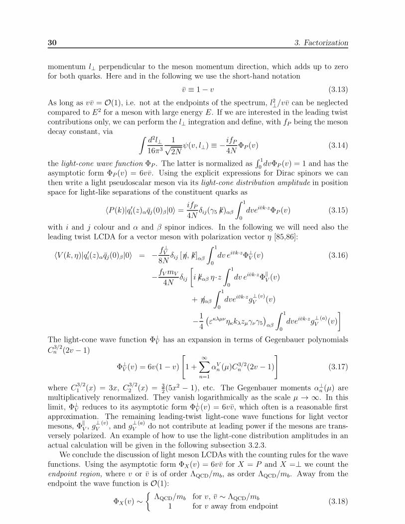
30 3. Factorization
momentum l⊥ perpendicular to the meson momentum direction, which adds up to zerofor both quarks. Here and in the following we use the short-hand notation
v ≡ 1− v (3.13)
As long as vv = O(1), i.e. not at the endpoints of the spectrum, l2⊥/vv can be neglectedcompared to E2 for a meson with large energy E. If we are interested in the leading twistcontributions only, we can perform the l⊥ integration and define, with fP being the mesondecay constant, via
∫d2l⊥16π3
1√2N
ψ(v, l⊥) ≡ −ifP4N
ΦP (v) (3.14)
the light-cone wave function ΦP . The latter is normalized as∫ 1
0dvΦP (v) = 1 and has the
asymptotic form ΦP (v) = 6vv. Using the explicit expressions for Dirac spinors we canthen write a light pseudoscalar meson via its light-cone distribution amplitude in positionspace for light-like separations of the constituent quarks as
〈P (k)|q′i(z)αqj(0)β|0〉 =ifP4N
δij(γ5 6k)αβ∫ 1
0
dveivk·zΦP (v) (3.15)
with i and j colour and α and β spinor indices. In the following we will need also theleading twist LCDA for a vector meson with polarization vector η [85,86]:
〈V (k, η)|q′i(z)αqj(0)β|0〉 = − f⊥V
8Nδij [6η, 6k]αβ
∫ 1
0
dv eivk·zΦ⊥V (v) (3.16)
−fVmV
4Nδij
[
i 6kαβ η ·z∫ 1
0
dv eivk·zΦ‖V (v)
+ 6ηαβ∫ 1
0
dveivk·zg⊥ (v)V (v)
−1
4
(εκλµνηκkλzµγνγ5
)
αβ
∫ 1
0
dveivk·zg⊥ (a)V (v)
]
The light-cone wave function Φ⊥V has an expansion in terms of Gegenbauer polynomials
C3/2n (2v − 1)
Φ⊥V (v) = 6v(1− v)
[
1 +
∞∑
n=1
αVn (µ)C
3/2n (2v − 1)
]
(3.17)
where C3/21 (x) = 3x, C
3/22 (x) = 3
2(5x2 − 1), etc. The Gegenbauer moments α⊥
n (µ) aremultiplicatively renormalized. They vanish logarithmically as the scale µ → ∞. In thislimit, Φ⊥
V reduces to its asymptotic form Φ⊥V (v) = 6vv, which often is a reasonable first
approximation. The remaining leading-twist light-cone wave functions for light vectormesons, Φ
‖V , g
⊥ (v)V , and g
⊥ (a)V do not contribute at leading power if the mesons are trans-
versely polarized. An example of how to use the light-cone distribution amplitudes in anactual calculation will be given in the following subsection 3.2.3.
We conclude the discussion of light meson LCDAs with the counting rules for the wavefunctions. Using the asymptotic form ΦX(v) = 6vv for X = P and X =⊥ we count theendpoint region, where v or v is of order ΛQCD/mb, as order ΛQCD/mb. Away from theendpoint the wave function is O(1):
ΦX(v) ∼{
ΛQCD/mb for v, v ∼ ΛQCD/mb
1 for v away from endpoint(3.18)

3.2 QCD Factorization 31
B meson light-cone distribution amplitudes
The B-meson light-cone distribution amplitude appears in the hard-spectator interactionterm in (3.5), because a hard gluon can probe the momentum distribution of b andspectator quark inside the B meson. Compared to the light meson LCDAs we now haveone very heavy quark as constituent: The b quark carries the largest part of the B mesonsmomentum p: p+b = ξp+ ≈ p+, whereas for the spectator quark we have l+ = ξp+ withξ = O(ΛQCD/mb). From the explicit expression for a heavy quark and light antiquarkspinor we can pull out a factor ( 6 p + mB)γ5. In the B-meson rest frame the remainderis essentially proportional to 6 l since the spectator quark is neither energetic nor heavy,and thus no restrictions on the components of its spinor exist. However, we still want toperform the l⊥ integration and absorb it into the B-meson light-cone wave functions. Tothis end we decompose 6 l into a part proportional to 6n+ and 6n− where n is an arbitrarylight-like vector which can be chosen for example in the direction of one of the final stateparticle momenta. Our standard choice is n = n− = (1, 0, 0,−1). For this choice of n wedefine two scalar wave functions ΦB1/2 in the B meson light-cone distribution amplitudeas [15,87,88]:
〈0|bi(0)αqj(z)β |B(p)〉 = ifB4N
δij [( 6p+mb)γ5]αγ
∫ 1
0
dξ e−iξp+z−[ΦB1(ξ)+ 6nΦB2(ξ)]γβ (3.19)
This is the most general decomposition of the leading-power LCDA only if the transversemomentum of the spectator quark l⊥ can be neglected. The wave functions describethe distribution of light-cone momentum fraction ξ = l+/p+ of the spectator quark withmomentum l inside the B meson. They depend on the choice of n and are normalized as
∫ 1
0
dξ ΦB1(ξ) = 1
∫ 1
0
dξΦB2(ξ) = 0 (3.20)
Unfortunately, the B-meson wave functions are poorly known, even theoretically. Atscales much larger than mb they should approach a symmetric form as for light mesons.At scales of order mb and smaller, however, one expects the distribution to be highlyasymmetric with ξ = O(ΛQCD/mb).
What we will need later on besides the normalization conditions is the first negativemoment of ΦB1(ξ), which we parametrize by a quantity λB = O(ΛQCD), i.e.
∫ 1
0
dξΦB1(ξ)
ξ=mB
λB(3.21)
The counting for B mesons is different from the counting for light mesons. We usethe normalization condition (3.20) to get
ΦB1(ξ) ∼{mb/ΛQCD for ξ ∼ ΛQCD/mb
0 for ξ ∼ 1(3.22)
This represents the fact that it is practically impossible to find the light spectator quarkwith momentum of ordermb, because there is only a small probability for hard fluctuationsthat transfer a large momentum to the spectator. The same counting applies to otherheavy mesons.
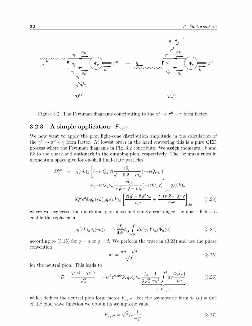
32 3. Factorization
vk
π0Φπ
vkk
q
p
vk
π0Φπ
vkk
q
p
D(q)1 D(q)
2
+qj
qj
qi
qi
Figure 3.2: The Feynman diagrams contributing to the γ∗ → π0 + γ form factor.
3.2.3 A simple application: Fγγπ0
We now want to apply the pion light-cone distribution amplitude in the calculation ofthe γ∗ → π0 + γ form factor. At lowest order in the hard scattering this is a pure QEDprocess where the Feynman diagrams in Fig. 3.2 contribute. We assign momenta vk andvk to the quark and antiquark in the outgoing pion, respectively. The Feynman rules inmomentum space give for on-shell final-state particles
D(q) = qj(vk)β
[
(−ieQq 6ǫ)iδji
6q − v 6k −mq(−ieQqγν)
+(−ieQqγν)iδji
v 6k− 6q −mq(−ieQq 6ǫ)
]
βα
qi(vk)α
= iQ2qe
2δjiqi(vk)αqj(vk)β
[ 6ǫ( 6q − v 6k)γνvq2
+γν(v 6k− 6q) 6ǫ
vq2
]
βα
(3.23)
where we neglected the quark and pion mass and simply rearranged the quark fields toenable the replacement
qi(vk)αqj(vk)β −→ ifπ4N
δij
∫ 1
0
dv(γ5 6k)αβΦπ(v) (3.24)
according to (3.15) for q = u or q = d. We perform the trace in (3.23) and use the phaseconvention
π0 =uu− dd√
2(3.25)
for the neutral pion. This leads to
D =D(u) −D(d)
√2
= −ie2εκλµνkκqλǫµγνfπ
3√2
1
−q2∫ 1
0
dvΦπ(v)
vv︸ ︷︷ ︸
≡ Fγγπ0
(3.26)
which defines the neutral pion form factor Fγγπ0 . For the asymptotic form Φπ(v) = 6vvof the pion wave function we obtain its asymptotic value
Fγγπ0 =√2fπ
1
−q2 (3.27)

3.2 QCD Factorization 33
Bd D+
π-
Figure 3.3: The leading-order contribution to the hard-scattering kernel T Iij in Bd →
D+π−. The pion’s momentum is k.
If one measures the form factor experimentally one can get information on the pionsvalence quark distribution.
3.2.4 One-loop proof of factorization in B → Dπ
In order to prove the validity of the factorization formulas (3.5) and (3.6), one has toshow that the hard scattering amplitudes T I
ij/k and T IIi are free of infrared singularities
to all orders in perturbation theory. For heavy-light final states such a proof exists at twoloops [15]. It has subsequently been extended to all orders [89]. We here only want tosketch the proof of factorization for B → Dπ at the one-loop order as given in the secondreference in [15].
The leading order
The relevant quark level decay for Bd → D+π− is b → cud so that no penguin operatorsor diagrams can contribute. At lowest order there is only a single diagram with no hardgluon interactions, shown in Fig. 3.3. The spectator quark is soft and absorbed as a softquark by the recoiling D meson which is described by the B → D form factor. Thehard subprocess is just given by the insertion of the colour-singlet four-fermion operatorOsinglet = cγµ(1 − γ5)b dγµ(1 − γ5)u. Therefore, it does not depend on the longitudinalmomentum fraction v of the two quarks that form the emitted π−. Consequently, withT Iij(v) being v-independent, the v-integral reduces to the normalization condition for the
pion wave function. So (3.6) reproduces the result of naive factorization if we neglectgluon exchange. In the heavy-quark limit the decay amplitude scales as
A(Bd → D+π−) ∼ GFm2bF
B→D(0)fπ ∼ GFm2bΛQCD (3.28)
Factorizable contributions
We now have to show that radiative corrections to Fig. 3.3 are either suppressed by αs
or ΛQCD/mb or are already contained in the definition of the form factor or the decayconstant of the pion. For example the first three diagrams in Fig. 3.4 are part of the formfactor and do not contribute to the hard-scattering kernels. In particular, the leadingcontributions from the region in which the gluon is soft (first and second diagram inFig. 3.4) are absorbed into the physical form factor. This is the one that appears in (3.5)and (3.6) and is also the one directly measured in experiments. The fourth diagram in

34 3. Factorization
Figure 3.4: Factorizable diagrams at O(αs) that are part of the form factor (first three
diagrams) or renormalize the conserved light-quark V −A current (last diagram).
(v1) (v2) (v3) (v4)
Figure 3.5: “Non-factorizable” vertex corrections.
Fig. 3.4 simply renormalizes the conserved (ud) light-quark V−A current and cancels thewave-function renormalization of the quarks in the emitted pion.
“Non-factorizable” vertex corrections
The diagrams containing gluon exchanges that do not belong to the form factor for theB → D transition or the pion decay constant are called “non-factorizable”.
The vertex corrections of Fig. 3.5 violate the naive factorization ansatz (3.1). Nev-ertheless they are calculable and form an O(αs) correction to the hard-scattering kernelT Iij(u). Although the diagrams in Fig. 3.5 exhibit seperately a collinear and soft infrared
divergence, we can show that these divergences cancel in the sum of all four diagrams. Thecancellation of the soft divergences is a manifestation of Bjorken’s colour-transparency ar-gument and the collinear divergences cancel due to collinear Ward identities. So the sumof the four diagrams involves only hard-gluon exchange at leading power.
At O(αs) the only vertex correction in Bd → D+π− comes from the colour-octetoperator Ooctet = cγµ(1 − γ5)T
ab dγµ(1 − γ5)Tau. We choose the quark and antiquark
momentum in the pion as
l1 = vk + l⊥ +~l2⊥4vE
n− l2 = vk − l⊥ +~l2⊥4vE
n− (3.29)
with k = E(1, 0, 0, 1) the pion momentum, E = pb · k/mB the pion energy, and n− =(1, 0, 0,−1). We want to show that the transverse momentum l⊥ can be neglected atleading power and that the contributions from the soft-gluon region and from gluonscollinear to k are power suppressed. As we have to keep l⊥ for the moment we use (3.15)before the l⊥ integration in (3.14):
〈π(k)|u(z)αd(0)β|0〉 =∫
dvd2l⊥16π3
1√2N
ψ∗(v, l⊥)(γ5 6k)αβeil1·z (3.30)
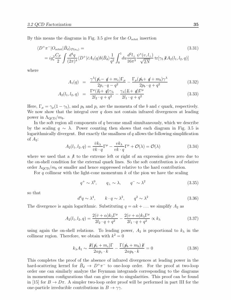
3.2 QCD Factorization 35
By this means the diagrams in Fig. 3.5 give for the Ooctet insertion
〈D+π−|Ooctet|Bd〉O(αs) = (3.31)
= ig2sCF
2
∫d4q
(2π)4〈D+|cA1(q)b|Bd〉
1
q2
∫ 1
0
dud2l⊥16π3
ψ∗(v, l⊥)√2N
tr[γ5 6kA2(l1, l2, q)]
where
A1(q) =γλ( 6pc− 6q +mc)Γµ
2pc · q − q2− Γµ( 6pb+ 6q +mb)γ
λ
2pb · q + q2(3.32)
A2(l1, l2, q) =Γµ( 6 l2+ 6q)γλ2l2 · q + q2
− γλ( 6 l1+ 6q)Γµ
2l1 · q + q2(3.33)
Here, Γµ = γµ(1− γ5), and pb and pc are the momenta of the b and c quark, respectively.We now show that the integral over q does not contain infrared divergences at leadingpower in ΛQCD/mb.
In the soft region all components of q become small simultaneously, which we describeby the scaling q ∼ λ. Power counting then shows that each diagram in Fig. 3.5 islogarithmically divergent. But exactly the smallness of q allows the following simplificationof A2:
A2(l1, l2, q) =vkλvk · qΓ
µ − vkλvk · qΓ
µ +O(λ) = O(λ) (3.34)
where we used that a 6 k to the extreme left or right of an expression gives zero due tothe on-shell condition for the external quark lines. So the soft contribution is of relativeorder ΛQCD/mb or smaller and hence suppressed relative to the hard contribution.
For q collinear with the light-cone momentum k of the pion we have the scaling
q+ ∼ λ0, q⊥ ∼ λ, q− ∼ λ2 (3.35)
so thatd4q ∼ λ4, k · q ∼ λ2, q2 ∼ λ2 (3.36)
The divergence is again logarithmic. Substituting q = αk + . . . we simplify A2 as
A2(l1, l2, q) =2(v + α)kλΓ
µ
2l2 · q + q2− 2(v + α)kλΓ
µ
2l1 · q + q2∝ kλ (3.37)
using again the on-shell relations. To leading power, A2 is proportional to kλ in thecollinear region. Therefore, we obtain with k2 = 0
kλA1 ∼6k( 6pc +mc)Γ
2αpc · k− Γ( 6pb +mb) 6k
2αpb · k= 0 (3.38)
This completes the proof of the absence of infrared divergences at leading power in thehard-scattering kernel for Bd → D+π− to one-loop order. For the proof at two-looporder one can similarly analyze the Feynman integrands corresponding to the diagramsin momentum configurations that can give rise to singularities. This proof can be foundin [15] for B → Dπ. A simpler two-loop order proof will be performed in part III for theone-particle irreducible contributions in B → γγ.

36 3. Factorization
Figure 3.6: Penguin diagram and chromomagnetic dipole operator contribution to B →M1M2.
Figure 3.7: “Non-factorizable” spectator interactions.
As |l⊥| ≪ E we can expand A2 in |l⊥|/E, which amounts to simply neglecting l⊥altogether. Then l1 = vk and l2 = vk, and we again can use the l⊥ integrated pion wavefunction (3.14) to simplify the matrix element of Ooctet in (3.31) to
〈D+π−|Ooctet|Bd〉O(αs) =
= −g2sCF
8N
∫d4q
(2π)4〈D+|cA1(q)b|Bd〉
1
q2fπ
∫ 1
0
dvΦπ(v)tr[γ5 6kA2(vk, vk, q)] (3.39)
∝ FB→D(0)
∫ 1
0
dv Toctet(v, z)Φπ(v) (3.40)
where z = mc/mb, FB→D(0) is the form factor that parametrizes the 〈D+|c[. . .]b|Bd〉
matrix element, and Toctet(v, z) is the hard-scattering kernel whose epxlicit expressioncan be found in [15].
Penguin diagrams
In general, a non-leptonic B decay can also get contributions from penguin diagramsand the chromomagnetic dipole operator Q8 as depicted in Fig. 3.6 They would bothgive calculable O(αs) corrections to the hard-scattering kernel T I
ij(u). For Bd → D+π−
however, neither of the two contributions exists because of the flavour structure of thefinal state.
Hard spectator interaction
In (3.6) we claimed that there is no contribution from hard-spectator interaction to heavy-light final states at leading power in the heavy-quark expansion. Soft contributions fromdiagrams in Fig. 3.7 cannot be absorbed into the B → D form factor or the pion decayconstant. For factorization to hold true, no such soft contributions may appear at leadingpower. Although they are present in each of the two diagrams separately, to leading power

3.2 QCD Factorization 37
(a1) (a2) (a3) (a4)
Figure 3.8: Annihilation topologies.
they cancel in the sum over the two gluon attachments to the ud pair by the same colour-transparency argument that was applied to the “non-factorizable” vertex corrections.Power counting for the summed amplitude of the two diagrams shows explicitely thepower suppression relative to (3.28).
Annihilation topologies
Finally, we will recall the power suppression of both hard and soft part of annihilationtopologies as in Fig. 3.8. According to (3.22) the light quark that goes into the D mesonmust always be soft. Therefore, the virtuality of the gluon can be at most mbΛQCD. Thepotentially largest contribution can be achieved if both quarks the gluon splits into aresoft. This configuration, however, is power suppressed via the pion wave function integral.
3.2.5 Limitations of QCD factorization
The factorization formulas (3.5) and (3.6) are exact in the heavy-quark limit mb → ∞.This is a theoretically very well defined limit. In the real world, on the other hand, mb
is fixed to about 4− 5GeV and one may question the accuracy of the heavy-quark limit.The generic size of power corrections is O(ΛQCD/mb) ≈ O(10%). Yet, sometimes powercorrections turn out to be numerically larger than suggested by this naive estimate.
Due to a conspiracy of small parameters, like Wilson coefficients, CKM elements, orcolour suppression factors, the leading-power, factorizable term can be somehow sup-pressed, making power corrections disproportionately large. A related issue is that thestrong-interaction phases appearing at O(αs) in QCD factorization might receive largecorrections from soft phases of O(ΛQCD/mb), because αs and ΛQCD/mb are of comparablesize.
Especially for B decays into two two light mesons there sometimes is another enhance-ment of power-suppressed effects connected with the curious numerical fact that
2µπ ≡ 2m2π
mu +md≈ 3GeV (3.41)
is much larger than its naive scaling estimate ΛQCD. The Q6 contribution to the diagram inFig. 3.3 for Bd → π+π− is an example for such a chirally enhanced power correction. Suchnumerically large corrections introduce a substantial uncertainty in some decay modes.
The last point we want to mention is the hybrid role of the charm quark. In our powercounting we treated the charm quark as heavy, taking the heavy-quark limit for fixedmc/mb. However, in reality mc is not markedly large compared to ΛQCD. In particular,the power suppression of the hard-spectator term in (3.6) for B decays into a heavy anda light meson is ΛQCD/mc only, if one employs the limit mb ≫ mc ≫ ΛQCD.

38 3. Factorization
Although the issue of power corrections still deserves thorough investigation we believethat the QCD factorization approach is a big step forward in the treatment of exclusiveB decays. For the first time we really have a method based on solid theoretical grounds,namely the heavy-quark limit. Time will show if its phenomenological value is comparable.Proposals of how to estimate or even measure the up to now unknown power correctionsare already on the market [90,91] and more work on this subject is expected.
3.3 Other Approaches to Non-Leptonic Decays
We conclude this chapter with a mini review of attempts to treat hadronic matrix ele-ments in non-leptonic B decays. Some different formulations and generalizations of thenaive factorization idea were presented already in section 3.1. In these approaches asmall set of phenomenological parameters is introduced in order to parametrize impor-tant non-factorizable effects. Yet, no attempt is made to calculate these parameters fromfirst principles. Another class of approaches aims at a dynamical understanding of non-leptonic weak decays starting from QCD and making a controlled set of approximations.The third class, finally, is based on classifications in terms of flavour topologies or Wickcontractions. We now will briefly discuss some representatives of the second and thirdclass of approaches.
3.3.1 Dynamical approaches
QCD is a beautiful and most probably even the correct theory to describe strong interac-tion effects in weak decays of hadrons. Still, the main drawback of QCD is that it is notyet solved in the nonperturbative domain. So, especially for the study of non-perturbativeproperties of QCD, many more or less well-defined approximations were invented to getinsight into QCD dynamics at least in some limiting situations.
Large-N expansion
QCD simplifies substantially in the limit of a large number N of colour degrees of free-dom [92]. One can treat SU(N) QCD as a theory of weakly interacting mesons, andan expansion in 1/N then amounts to a loop expansion in this meson theory [93]. Mostimportant for us is that the factorization of non-leptonic decay amplitudes becomes exactin the large-N limit. Hence, an expansion in powers of 1/N provides a natural frameworkin which to discuss the structure of non-factorizable corrections. For kaon decays a com-bination of the 1/N expansion with chiral perturbation theory led to important insightinto non-factorizable effects [94]. For B decays, however, chiral perturbation theory doesnot apply. Still, one can use the large-N limit to show that non-factorizable correctionsto class-I B decays are generally suppressed by two powers of 1/N , whereas for class-IIdecays they have the same 1/N scaling as the leading factorizable contribution.
Lattice gauge theory
Although lattice field theory is the carrier of hope for many non-perturbative problems,no real results have been obtained so far in the evaluation of exclusive non-leptonic matrixelements. The Maiani-Testa No-go theorem [95] even forbade lattice QCD to calculate

3.3 Other Approaches to Non-Leptonic Decays 39
the matrix elements for non-leptonic two-body decays from first principles until Lellouchand Luscher found a way to possibly still do so [96]. Yet, there are still many technicaldifficulties with lattice QCD and non-leptonic B decays, in particular concerning final-state interactions and the inclusion of penguin diagrams.
QCD sum rules
Although intrinsically limited in their numerical accuracy, in many areas QCD sum ruleshave been established as a serious competitor to lattice gauge theory computations. Inparticular for the form factors at large recoil, QCD sum rules might be equal or evensuperior to lattice results for still some time. Some attempts were made to apply QCDsum rules to non-leptonic weak decays [97]. Non-factorizable effects were studied forB → J/ψKS [98] and Bd → D0π0 [99]. Recently, Khodjamirian suggested to study powercorrections for two-body B decays in the framework of light-cone QCD sum rules [90]. Animportant conceptual limitation for QCD sum rules in non-leptonic decays is that it willnot be possible to obtain a realistic description of final-state interactions if the projectionon the external hadron state is performed using an ad hoc continuum subtraction.
Large-energy effective theories
Dugan and Grinstein tried to formalize the concept of colour transparency by introducinga large-energy effective theory (LEET) to describe the soft interactions of gluons witha pair of fast-moving quarks inside a pion [76]. Yet, due to the presence of collinearsingularities, the LEET is not the correct low-energy theory for non-leptonic B decays.In the context of the LEET effective Lagrangian no light-cone distribution amplitudes canbe introduced to absorb the factorizable collinear singularities. We refer to [88,100,101]for further developments of “LEET.”
PQCD
The goal of perturbative QCD (pQCD) or other hard-scattering approaches is likewisethe separation of soft and hard physics in the B-decay matrix element [102]. Similarto QCD factorization the decay amplitudes are expressed as a convolution of a hard-scattering amplitude and meson wave functions. Yet, there are fundamental differencesin the details. In the pQCD approach the B → M form factors are assumed to beperturbatively calculable. It is postulated that soft contributions to the form factors arestrongly suppressed by Sudakov effects. The form factor is then counted as being of O(αs)in perturbation theory, and thus the hierarchy of the various contributions to the decayamplitudes in pQCD is very different from that in QCD factorization. One consequencehereof is that naive factorization is not recovered in any limit.
Especially for the claim that Sudakov effects suppress long-distance contributions suf-ficiently for the form factors to be calculable reliably and precisely in perturbation theory,serious doubts were raised [103]. Furthermore, the estimate of the strong-interaction phasewithin pQCD is both model dependent and numerically sensitive to effects that are poorlyunder control [15].

40 3. Factorization
ECT
A P PA
Figure 3.9: The six building blocks of the diagrammatic way: Tree emission of an external
W boson (T ); internal colour-suppressed W emission (C); Exchange of the W boson
between the quark lines of the initial state meson (E); annihilation of the B meson and
subsequent decay of the W boson into the final state particles (A); penguin diagram with
a “horizontal” W exchange (P ); penguin annihilation (PA).
3.3.2 The diagrammatic way and flavour symmetry approaches
There exist several strategies to classify the various contributions to non-leptonic weakdecay amplitudes in a convenient way, and then to use symmetry arguments to deriverelations between different decay processes. We shall briefly discuss the diagrammaticapproach, a parametrization introduced by Buras and Silvestrini, and a flavour SU(3)decomposition of decay amplitudes.
The diagrammatic way
Especially for the description of charmless non-leptonic two-body decays of B mesons thesix diagrams in Fig. 3.9 were used [104]. Because the amplitudes A, PA, and E are sup-pressed with at least one factor of 1/(mass of the decaying heavy meson) compared withT , C, and P , they are often neglected altogether. The fact that no explicit conntection tothe effective theory of weak interaction exists is also a disadvantage. Instead, Feynmandiagrams with propagators in the full theory are used. But this describes the situationat large scales O(MW ) rather than at the much better suited mass scale of the decayingheavy meson.
The parametrization of Buras and Silvestrini
The basis for the parametrization of Buras and Silvestrini (BS) are Wick contractions ofthe effective Hamiltonian H∆B=1
eff [105]. The different topologies arise from the differentpossibilities to connect the quark lines of the initial and final state mesons, taking intoaccount the operator insertion. One obtains seven different topologies, which appearin a connected and disconnected version each. This leads to fourteen renormalizationscale and scheme independent parameters, which allow to describe all amplitudes for non-

3.3 Other Approaches to Non-Leptonic Decays 41
M1
q2
q1
M2
B
b q2q3
q1
Qi
BQi
CE i(q3, q2, q1;B,M1,M2)DE i(q3, q2, q1;B,M1,M2)
M1
M2
b
q3
Figure 3.10: Disconnected and connected emission topology leading to the parameters
DE and CE , respectively. The dashed lines represent insertions of the operators Qi.
leptonic two-body decays of B mesons. An example for the simplest topology leading tothe parameters DE and CE is given in Fig. 3.10. The matrix elements of the operatorsQi depend on the renormalization scale and scheme for the operators which has to becancelled by a corresponding dependence of the Wilson coefficients. Usually, severaloperators are involved in this cancellation as the operators mix under renormalization.The fourteen effective parameters of Buras and Silvestrini are linear combinations ofoperator matrix elements and corresponding Wilson coefficients. Insertion of Q1 and Q2
into DE and CE topologies of Fig. 3.10 yields the first two scale and scheme independentcombinations of Wilson coefficients and operator matrix elements:
E1 = C1DE 1 + C2CE 2
E2 = C1CE 1 + C2DE 2 (3.42)
which are generalizations of aeff1 〈Q1〉 and aeff2 〈Q2〉 in [80] and (3.3). Since all BS param-eters are combinations of Wilson coefficients and special contractions of local operators,they are in principle calculable in QCD. Unfortunately, so far the BS parametrization is inparticular because of the large number of parameters only of limited use for phenomeno-logical analyses. In combination with a dynamical approach such as QCD factorization,however, one could obtain model-independent predictions for special decay channels ormake statements about the relative importance of the various BS parameters.
SU(3) flavour symmetry
Compared with the typical scale of QCD Λ(4)
MS≈ 325MeV, the masses of the light quarks
mu ≈ 5MeV, md ≈ 10MeV, and, less exactly, ms(mc) ≈ 130MeV are small and approx-imately degenerate. Because the strong interaction is flavour blind, it therefore satisfiesa flavour-SU(3) symmetry, which is explicitely broken via the inexact mass degeneracy.This symmetry property was used both for D- and B-meson decays to determine forinstance CKM elements from experimental data [106,107].
Let us consider the decay B → PP as an example. We follow the conventions of [108].The Hamilton operator H∆B=1
eff connects the B mesons in the initial state i with the twopseudoscalar mesons P in the final state f . In view of the SU(3)-flavour symmetry themost general interaction Hamiltonian is composed of the representations R appearing in
42 3. Factorization
f ⊗ i. The i and f denote here both states and SU(3) representations. A completelyreduced SU(3) amplitude can be denoted by 〈f‖RI‖i〉 where I denotes the eigenvalueof the isospin Casimir operator I2. Due to Bose statistics we only have to consider thecompletely symmetric representations for a B decay into two light pseudoscalar octetmesons:
(8⊗ 8)S = 1⊕ 8S ⊕ 27 (3.43)
The physical amplitude for the decay of a particle of the SU(3) representation Rc withquantum numbers νc into two particles of the representation Ra and Rb with quantumnumbers νa and νb, respectively, can be decomposed into the reduced matrix elements asfollows:
A(iRcνc → fRa
νa fRbνb) = (3.44)
= (−1)(I3+Y2+T
3)Rc
∑
R′,ν′,R,ν
(Ra Rb R′
νa νb ν ′
)(R′ Rc Rν ′ −νc ν
)
〈R′‖Rν‖Rc〉
where the triality T guarantees the reality of the phase factor. The quantities in roundbrackets are Clebsch-Gordan coefficients. They connect, via the Wigner-Eckart theorem,the irreducible tensor operators in-between two states, which are base vectors of irreduciblerepresentations. Because the Clebsch-Gordan matrices are orthogonal, the reduced SU(3)amplitudes build an orthonormal basis. In a decomposition of amplitudes, ordered byparticle content of the final state, and then by the number of units of strangeness changed,as e.g.
u∆S=0B→PP = O∆S=0
B→PPv∆S=0B→PP (3.45)
the matrices O∆SB→f thus are orthogonal. This implies that the reduced SU(3) amplitudes
v∆S=0B→PP are related with the decay amplitudes u∆S=0
B→PP via the transposed of O∆S=0B→PP . If
there is a physical reason for a reduced SU(3) amplitude to vanish, the correspondingcombination of physical amplitudes also vanishes. For ∆S = 0 B → PP decays forexample, no matrix elements with representations 24 or 42 can contribute in the limit ofexact SU(3)-flavour symmetry. There are five such reduced SU(3) amplitudes, leading tofive amplitude relations, the simplest of them being the isospin relation
−√2A(B+
u → π+π0) + A(B0d → π+π−) +
√2A(B0
d → π0π0) = 0 (3.46)
Similar relations can be derived for D decays [109].

Part II
The Radiative Decays B → V γ at
NLO in QCD


Chapter 4
Basic Formulas for B → V γ
The second part is devoted to the analysis of the exclusive radiative B-meson decays witha vector meson V in the final state, i.e. in particular the decays B → K∗γ and B → ργ.We present a factorization formula for the B → V γ matrix elements, which is based onthe heavy-quark limit mb ≫ ΛQCD. This allows us to factorize perturbatively calcula-ble contributions from nonperturbative form factors and universal light-cone distributionamplitudes. Our results are complete to next-to-leading order in QCD and to leadingpower in the heavy-quark limit and include the branching ratios and estimates of directCP violation, isospin and U-spin breaking effects. In chapter 4 we present the structureof the QCD factorization formulas. These formulas are applied to B → K∗γ and B → ργin chapter 5. The results given here have to a great extent already been presented in[110]. We go more into detail in the work on hand, add a proof for the factorizability ofannihilation contributions, and, above all, include the effects of QCD penguin operators.
4.1 What is the Problem?
The radiative transitions b → sγ and b → dγ are among the most valuable probes offlavour physics. Proceeding at rates of order G2
Fα, they are systematically enhanced overother loop-induced, non-radiative, rare decays, which are proportional to G2
Fα2. In fact,
the Cabibbo-favoured b → sγ modes belong to the small number of rare decays thatare experimentally accessible already at present. The experimental measurement of theinclusive branching fraction was quoted already in (2.69). The branching ratios for theexclusive channels have been determined by CLEO [68] and more recently also by BELLE[70] and BaBar [111]:
B(B0 → K∗0γ)exp. =
(4.55± 0.70± 0.34) · 10−5 [68](4.96± 0.67± 0.45) · 10−5 [70](4.23± 0.40± 0.22) · 10−5 [111]
(4.1)
B(B+ → K∗+γ)exp. =
(3.76± 0.86± 0.28) · 10−5 [68](3.89± 0.93± 0.41) · 10−5 [70](3.83± 0.62± 0.22) · 10−5 [111]
(4.2)

46 4. Basic Formulas for B → V γ
Although for the B → ργ decays so far only upper limits exist [112], they are alreadyvery close to the Standard Model expectations:
B(B0 → ρ0γ) < 1.5 · 10−6 at 90% C.L.B(B+ → ρ+γ) < 2.8 · 10−6 at 90% C.L.
(4.3)
On the theoretical side, the flavour-changing-neutral-current (FCNC) reactions b→ s(d)γare characterized by their high sensitivity to New Physics and by the particularly largeimpact of short-distance QCD corrections [47–51].
As we already mentioned in section 2.5, the inclusive b → sγ mode can be calculatedperturbatively, whereas the treatment of the exclusive channels is in general more com-plicated. Seen from the experimental point of view, however, the situation is the oppositeway round. Measurements of inclusive rates are rather difficult to perform, as one hasto sum over all final states containing e.g. a photon and a strange quark. Furthermore,a lower cutoff in the photon energy has to be imposed in order to get along with thebackground coming mainly from the nonleptonic charged current processes b→ c/u qq γ.Theoretical input on the photon energy spectrum is then needed to translate the measured“kinematic” branching ratio into the total one. The exclusive decays, on the other hand,show a very clean experimental signature, which is particularly important for the difficultenvironment of hadron machines as the Fermilab Tevatron or the LHC at CERN. Onceagain the conservation law, that “the product of theoretical difficulty and experimentaleffort needed to solve a problem is constant,” seems to hold.
The main difficulty in calculations of exclusive hadronic decays is how to evaluate thematrix elements of the operators sandwiched between final V γ and initial B state. Thesematrix elements lump together all the nonperturbative long-distance dynamics below ascale of O(mB). From Lorentz covariance and gauge invariance, the B → V γ transitionmatrix elements have the following general form
〈V (k, η)γ(q, ǫ)|Qi|B〉 = − e
2π2mBFV (0)
[εµνλρǫµηνkλqρ + i(ǫ · η k · q − ǫ · k η · q)
](4.4)
This is just a convenient parametrization in terms of the form factor FV (q2 = 0), which
constitutes now the challenge to be determined. For q2 6= 0, i.e. an off-shell photon,we have two form factors: one in front of each of the two terms in (4.4), which aregauge invariant separately. The form factors are calculable in principle from lattice QCD[113]. Since the lattice calculations provide results over a limited region of high q2, i.e.small recoil, extra assumptions are needed to scale down the form factors to the case ofan onshell external photon with q2 = 0. Via the light-cone sum-rule (LCSR) approach[84,114] a more direct access to the q2 = 0 region is opened [86,115]. But the theoreticalaccuracy of sum rule calculations is, due to the duality approximation made, irreduciblyrestricted to O(10%). There are further prescriptions on the market how to include boundstate effects in B → V γ [116,117]. However, hadronic models are used which do not allowa clear separation of short- and long-distance dynamics and a clean distinction of model-dependent and model-independent features. In section 5.2 we comment on these andrelated calculations in the context of QCD factorization.

4.2 The Factorization Formula 47
Figure 4.1: Contribution of the magnetic penguin operator Q7 described by B → V form
factors. All possible gluon exchanges between the quark lines are included in the form
factors and have not been drawn explicitly.
4.2 The Factorization Formula
In the heavy-quark limit, a systematic treatment of the hadronic matrix element is possible[110,118,119]. In this case, the following factorization formula is valid
〈V γ(ǫ)|Qi|B〉 =[
FB→V (0) T Ii +
∫ 1
0
dξ dv T IIi (ξ, v) ΦB(ξ) ΦV (v)
]
· ǫ (4.5)
where ǫ is the photon polarization 4-vector. With the B → V transition form factor FB→V
and ΦB and ΦV , the leading twist light-cone distribution amplitudes of the B meson andthe vector meson, respectively, we encounter universal, nonperturbative objects. Theydescribe the long-distance dynamics of the matrix elements, which is factorized fromthe perturbative, short-distance interactions expressed in the hard-scattering kernels T I
i
and T IIi . The QCD factorization formula (4.5) holds for all operators in (2.50–2.65) up
to corrections of relative order ΛQCD/mb. We include the calculable contributions ofall operators unless they are both of subleading power and suppressed by αs(µb) withµb = O(mb).
In the leading-logarithmic approximation and to leading power in the heavy-quarklimit, Q7 gives the only contribution to the amplitude of B → V γ, and the factorizationformula (4.5) is trivial. The matrix element is simply expressed in terms of the standardform factor, T I
7 is a purely kinematical function, and the spectator term T II7 is absent.
An illustration is given in Fig. 4.1. The matrix element reads
〈V (k, η)γ(q, ǫ)|Q7|B〉 = − e
2π2mb cV FV
[εµνλρǫµηνkλqρ + i(ǫ · η k · q − ǫ · k η · q)
](4.6)
where cV = 1 for V = K∗, ρ− and cV = 1/√2 for V = ρ0. Our phase conventions coincide
with those of [86,115]. In particular, we have FV > 0, ε0123 = −1, and the phases of V(with flavour content qq′) and B are such that
〈V (k, η)|qσµνq′|0〉 = −i(ηµkν − ηνkµ)f⊥V (4.7)
〈0|uγµγ5b|B(p)〉 = +ifBpµ (4.8)
with positive fB, f⊥V .
Only at O(αs) the matrix elements of the other seven operators start contributing.In this case the factorization formula becomes nontrivial. The diagrams for the “type

48 4. Basic Formulas for B → V γ
Figure 4.2: O(αs) contribution to the hard-scattering kernels T Ii from four-quark oper-
ators Q1...6. The crosses indicate the places where the emitted photon can be attached.
Diagrams where the gluon is exchanged in the loop vanish for the same reason as the
mixing of Q1...4 into Q7 vanishes at one-loop level: chirality conservation in the quark
loop and QED gauge invariance.
Figure 4.3: O(αs) contribution to the hard-scattering kernels T I8 from chromomagnetic
penguin operator Q8.
I” or “hard vertex” contributions are shown in Fig. 4.2 for Q1...6 and in Fig. 4.3 forQ8. The calculation of these diagrams leads to infrared-finite functions of mq/mb, wheremq is the mass of the internal quarks in the loop diagram. The “type II” or “hardspectator” contributions are those where the B-meson-spectator quark participates inthe hard scattering. The non-vanishing contributions to T II
i are shown in Fig. 4.4. Thehard gluon therein probes the momentum distribution of the quarks in the B meson andthe light vector meson. To evaluate these diagrams we need the light-cone distributionamplitudes (LCDA) of the participating mesons. In the case of the B meson we have toleading power the formula given in (3.19). If we choose n in (3.19) appropriately, we needbesides the normalization conditions only the first negative moment of ΦB1(ξ), whichwe parametrized by the quantity λB in (3.21). The vector meson in B → V γ decaysis transversly polarized to leading power. This can be described by Φ⊥, the leading-twist and leading-power distribution amplitude for a light vector mesons with transversepolarization, defined by the first line in equation (3.16):
〈V (k, η)|q′i(z)αqj(0)β|0〉 = − f⊥V
8Nδij [ 6η, 6k]αβ
∫ 1
0
dv eivkxΦ⊥(v) (4.9)
The diagrams in Figs. 4.1–4.4 are not yet the complete set of possible contributionsto B → V γ decays. One of the further possibilities is weak annihilation, depicted inFig. 4.5. If we calculate this contribution for Q1...4 using the leading-power projectiononto the meson V in (4.9) we get a vanishing result because the trace over an odd number

4.2 The Factorization Formula 49
s; d
b
Figure 4.4: O(αs) contribution to the hard-scattering kernels T IIi from four-quark opera-
tors Qi (left) and from Q8 (right).
+
Q5,6
b
Q5,6+
+
Q1...4
Figure 4.5: Annihilation contribution to the B → V γ decay. The dominant mechanism
for operators Q1...4 is the radiation of the photon from the light quark in the B meson, as
shown. This amplitude is suppressed by one power of ΛQCD/mb, but it is still calculable
in QCD factorization. Radiation of the photon from the remaining three quark lines is
suppressed by (ΛQCD/mb)2 for operators Q1...4. For operators Q5,6, however, radiation
of the final state vector meson quarks is power suppressed diagrammatically but gives a
contribution from the leading power projector.
of Dirac matrices is zero. Yet, a non-vanishing result arises from the projector
〈V (k, η)|qγνq′|0〉 = fVmV ην (4.10)
which, however, is suppressed by one power of ΛQCD/mb compared to (4.7), (4.9) fortransverse polarization ην (fV , f
⊥V , mV ∼ ΛQCD, k ∼ mb). For operators Q5,6 one gets a
contribution from the leading power projector when the photon is emitted from the finalstate vector meson, which is power suppressed diagrammatically. Hence, weak annihila-tion contributions are power suppressed. When the photon is not emitted as in Fig. 4.5,the annihilation contributions are either vanishing or even stronger suppressed becausethe quark propagators are scaling as 1/mb instead of 1/ΛQCD and only the subleadingprojector appears..
Despite their power suppression, the dominant annihilation amplitudes can be com-puted within QCD factorization. For the explicit proof to O(αs) we refer to Appendix C.Physically, the annihilation contributions factorize because the colour-transparency argu-ment applies to the emitted, highly energetic vector meson in the heavy-quark limit [15].A similar observation was already made in [120]. Grinstein and Pirjol, however, claimthat the O(αs) corrections to Fig. 4.5 would vanish identically in the chiral limit and to

50 4. Basic Formulas for B → V γ
s; d
b
Figure 4.6: Other contributions that are power-suppressed in the heavy-quark limit. The
penguin-annihilation diagrams (left) can be calculated in QCD factorization, but for the
subleading-power Q8 matrix elements (right) where the photon is emitted from the final
state vector meson, factorization breaks down.
leading-twist, because the projector in (4.9) gives zero when applied to a current with anodd number of Dirac matrices. But, by the same argument, the diagram in Fig. 4.5 wouldvanish even at leading order in αs, which is not the case. The proper treatment of theO(αs) correction for Q1,2 should employ the subleading-power projections related to the
wave functions Φ‖V , g
⊥ (v)V , g
⊥ (a)V [85,86], corresponding to the use of (4.10) at O(α0
s).Since weak annihilation is a power correction, we will content ourselves with the lowest
order result (O(α0s)) for our estimates below. In particular, we shall use the annihilation
effects to estimate isospin-breaking corrections in B → V γ decays. The reason for includ-ing this class of power corrections is that they come with a numerical enhancement fromthe large Wilson coefficients C1,2 (C1 ≈ 3|C7|) or are numerically enhanced in case of theQ5,6 penguin operator contributions.
Finally, Fig. 4.6 displays the remaining diagrams with a power suppression. Thepenguin-annihilation diagrams (left) are power suppressed in a way similar to the ordinaryannihilation topologies. They are additionally suppressed by αs. The spectator diagramsfrom Q8 (right) lead to amplitudes that are either manifestly power-suppressed (photonemitted from the quark line in the upper right) or that are superficially of leading power,but vanish when the leading-order projections are performed (photon emitted from eitherof the quarks forming the B meson). Recall, however, that photon emission from thelight-quark line from Q8 is a leading-power effect (see Fig. 4.4).
4.3 The Hard Vertex Corrections
To O(αs) the amplitude for B → V γ reads, with the short-hand notation 〈Qi〉 ≡〈V γ|Qi|B〉, for our standard or the CMM operator basis
A(B → V γ) =GF√2
∑
p=u,c
λ(s)p
(
C1〈Q(p)1 〉+ C2〈Q(2)
2 〉+8∑
i=3
Ci〈Qi〉)
(4.11)
=GF√2
∑
p=u,c
λ(s)p
(
Z1〈P (p)1 〉+ Z2〈P (2)
2 〉+8∑
i=3
Zi〈Pi〉)

4.3 The Hard Vertex Corrections 51
The leading-order matrix element 〈P7〉 = 〈Q7〉 is given in (4.6). At subleading order in αs
the matrix elements 〈Q1...6,8〉 need to be computed from the diagrams in Figs. 4.2 – 4.4.We have to combine results of the matrix elements obtained in different operator bases:ours and the one of Chetyrkin, Misiak, and Munz (CMM). The final amplitude has tobe independent of the choice of an operator basis, of course. Even partial results whichhave a physical meaning have to be independent of the chosen operator basis. This willbe used subsequently. We will treat the type I contributions in the CMM (2.58–2.65) andthe type II contributions in our operator basis (2.50–2.57).
Let us now have a closer look at the type I or hard vertex contributions of Figs. 4.2and 4.3. The results for these diagrams can be inferred from [60–62]. In these papers thediagrams were computed to obtain the matrix elements for the inclusive mode b→ sγ atnext-to-leading order. In this context Figs. 4.2 and 4.3 represented the virtual correctionsto the inclusive matrix elements of Q1,8 [60] or P1...6,8 [62]. In our case they determinethe kernels T I
1...6 and T I8 . As required for the consistency of the factorization formula,
these corrections must be dominated by hard scales ∼ mb and hence must be infraredfinite. This is indeed the case. Only recently, Buras, Czarnecki, Misiak, and Urbancompleted the calculation of the NLO matrix elements including the penguin operators[62]. However, they calculated in the CMM basis. Nevertheless, we can re-interpretetheir results as the perturbative hard-scattering kernels for the exclusive process. This isbecause the NLO corrections to the matrix elements have a physical effect on the inclusiverate. For the exclusive decay the type I corrections are completely independent of thetype II contributions, which appear at O(αs) for the first time. Therefore, we can usedifferent operator bases for type I and type II corrections. The results from [62] imply
〈Pi〉I = 〈Q7〉αsCF
4πGi i 6= 7 (4.12)
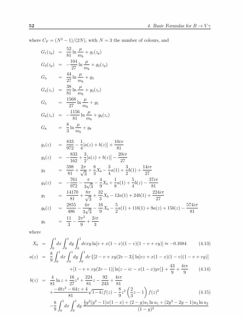
52 4. Basic Formulas for B → V γ
where CF = (N2 − 1)/(2N), with N = 3 the number of colours, and
G1(zp) =52
81ln
µ
mb+ g1(zp)
G2(zp) = −104
27ln
µ
mb+ g2(zp)
G3 =44
27ln
µ
mb
+ g3
G4(zc) =38
81ln
µ
mb+ g4(zc)
G5 =1568
27ln
µ
mb+ g5
G6(zc) = −1156
81ln
µ
mb+ g6(zc)
G8 =8
3ln
µ
mb+ g8
g1(z) =833
972− 1
4[a(z) + b(z)] +
10iπ
81
g2(z) = −833
162+
3
2[a(z) + b(z)]− 20iπ
27
g3 =598
81+
2π√3+
8
3Xb −
3
4a(1) +
3
2b(1) +
14iπ
27
g4(z) = −761
972− π
3√3− 4
9Xb +
1
8a(1) +
5
4b(z) − 37iπ
81
g5 =14170
81+
8π√3+
32
3Xb − 12a(1) + 24b(1) +
224iπ
27
g6(z) =2855
486− 4π
3√3− 16
9Xb −
5
2a(1) + 11b(1) + 9a(z) + 15b(z)− 574iπ
81
g8 =11
3− 2π2
9+
2iπ
3
where
Xb =
∫ 1
0
dx
∫ 1
0
dy
∫ 1
0
dvxy ln[v + x(1− x)(1− v)(1− v + vy)] ≈ −0.1684 (4.13)
a(z) =8
9
∫ 1
0
dx
∫ 1
0
dy
∫ 1
0
dv {[2− v + xy(2v − 3)] ln[vz + x(1− x)(1− v)(1− v + vy)]
+[1− v + xy(2v − 1)] ln[z − iε− x(1− x)yv]}+ 43
9+
4iπ
9(4.14)
b(z) =4
81ln z +
16
27z2 +
224
81z − 92
243+
4iπ
81
+−48z2 − 64z + 4
81
√1−4zf(z)− 8
9z2(2
3z − 1
)
f(z)2 (4.15)
−8
9
∫ 1
0
dx
∫ 1
0
dy12y2(y2 − 1)x(1− x) + (2− y)u1 ln u1 + (2y2 − 2y − 1)u2 ln u2
(1− y)2

4.3 The Hard Vertex Corrections 53
with uk = ykx(1 − x) + (1− y)z and
f(z) = θ(1−4z)
(
ln1 +
√1−4z
1−√1−4z
− iπ
)
− 2iθ(4z−1) arctan1√
4z−1(4.16)
The results for a(1) and b(1) read
a(1) ≃ 4.0859 +4iπ
9(4.17)
b(1) =320
81− 4π
3√3+
632π2
1215− 8
45
[d2 ln Γ(x)
dx2
]
x= 16
+4iπ
81≃ 0.0316 +
4iπ
81(4.18)
For z < 0.3 the functions a(z) and b(z) are very accurately given by their expansion in z:
a(z) = 169
{[52− π2
3− 3ζ(3) +
(52− 3π2
4
)
ln z + 14ln2 z + 1
12ln3 z
]
z
+[74+ 2π2
3− π2
2ln z − 1
4ln2 z + 1
12ln3 z
]
z2
+[
−76− π2
4+ 2 ln z − 3
4ln2 z
]
z3
+[457216
− 5π2
18− 1
72ln z − 5
6ln2 z
]
z4
+[351018640
− 35π2
72− 185
144ln z − 35
24ln2 z
]
z5
+[678018000
− 21π2
20− 3303
800ln z − 63
20ln2 z
]
z6
+iπ[(
2− π2
6+ 1
2ln z + 1
2ln2 z
)
z +(
12− π2
6− ln z + 1
2ln2 z
)
z2
+z3 + 59z4 + 49
72z5 + 231
200z6]}
+O(z7 ln2 z)
b(z) = −89
{(
−3 + π2
6− ln z
)
z − 2π2
3z3/2
+(12+ π2 − 2 ln z − 1
2ln2 z
)z2
+(
−2512
− π2
9− 19
18ln z + 2 ln2 z
)
z3
+[
−1376225
+ 13730
ln z + 2 ln2 z + 2π2
3
]
z4
+[
−13131711760
+ 88784
ln z + 5 ln2 s+ 5π2
3
]
z5
+[
−280761797200
+ 16597540
ln z + 14 ln2 z + 14π2
3
]
z6
+iπ[−z + (1− 2 ln z)z2 +
(−10
9+ 4
3ln z)z3 + z4 + 2
3z5 + 7
9z6]}
+O(z7 ln2 z)
We denote with
zq =m2
q
m2b
(4.19)
the squared ratio of the mass of the internal quark in the loop with respect to the b quarkmass.

54 4. Basic Formulas for B → V γ
bl si
q r+
bl si
r q
Figure 4.7: The building block for the Q1...6 contributions. The indices denote the colour
of the quarks. The other possible topology is a sq × qb instead of the sb × qq operator
insertion leading to diagrams with a continuous fermion line. It is equivalent to inserting
Fierz-transformed four-quark operators into the displayed topology.
4.4 The Hard Spectator Corrections
We now turn to the mechanism where the spectator participates in the hard scattering.To find the correction for 〈Q1...6〉 we compute the left diagrams in Fig. 4.4 using thelight-cone projectors in (3.19) and (4.9). We first calculate the “building blocks” Bαβ ofFig. 4.7. We obtain to leading power, with the photon on-shell and the gluon off-shell,
B(V −A)×(V∓A)αβ = ∓iQqgsT
ail
8π2ερστδγ
δγ5
(
gραgσβ (r
τ − qτ ) +rσqτ
q · r(gραqβ − gρβrα
))
(1− γ5)∆i
(4.20)for the insertion of a (V −A) × (V −A) operator, like in Q1...4, and a (V −A) × (V +A)structure, needed for Q5,6, respectively. The relative minus sign of the building block for(V−A)× (V−A) and (V−A)× (V +A) insertions can be easily understood using Furry’stheorem. Because a loop diagram with an odd number of vector currents vanishes, it isthe sign of the axialvector current inserted in the loop that determines the overall sign.The integral occuring in (4.20) is
∆i = 8 q · r∫ 1
0
dx
∫ x
0
dyxy
m2q − r2xx− 2r · q xy − iδ
(4.21)
The 1/ǫ pole of the building block vanishes in the naive dimensional regularization scheme.The use of this scheme is a priori not consistent for the topologies in figure 4.7 becausetraces with γ5 appear. Using another regularization scheme or calculating the correspond-ing topologies with a continuous fermion line will give a non-vanishing pole contribution.This, however, is mass independent and possible finite anomaly terms emerging from itwould be cancelled via the GIM mechanism. Therefore the result is indeed finite and wecan safely calculate in D = 4. We checked that the building block B
(V−A)×(V∓A)αβ is the
same when calculated with the Fierz-transformed operators inserted into the other possi-ble topology of Fig. 4.7. Apart from the fact that we set D = 4 already, kept the leadingpower part only, and an overall factor of 4 due to the definition of the operator basis, ourbuilding block B
(V−A)×(V −A)αβ is the same as Jαβ in [60]. The index α is contracted with
the photon polarization vector ǫα and β is the gluon index.For the QCD penguin operators we also have to consider the insertion of the Fierz-
transformed operators if q = s or q = b. One has the choice of inserting either both

4.4 The Hard Spectator Corrections 55
possible Fierz versions of a four-quark operator into one topology of a given diagram orone Fierz version into the two possible topologies. The result in the end is the same. Forthe topology in Fig. 4.7, however, we can relate the (V−A)× (V−A) and (V−A)× (V+A)operators via Furry’s theorem, which saves oneself the calculation of the diagrams with acontinuous fermion line. We still performed both calculations to cross-check.
A Fierz transformation of a (V−A)× (V−A) operator again gives a (V−A)× (V−A)operator. Therefore, we can use B
(V−A)×(V−A)αβ for insertions of Q3 and Q4. Yet, Fierz-
transforming Q5 = (sibl)V−A
∑
q(qjqk)V+A δilδkj leads to
QFierz5 = −2
∑
q
(siqk)S+P (qjbl)S−P δilδkj (4.22)
with the shorthand (q1q2)S±P := q1(1 ± γ5)q2. An insertion of such an operator (withoutthe sum over q) into the building block diagrams of Fig. 4.7 leads to
B(S+P )×(S−P )αβ = −
iQqgsTajl
2π2mq(1 + γ5)
[(qβrαq · r − gαβ
)
∆i (4.23)
+(q · rgαβ − rαqβ − iε(q, r, γα, γβ))∆j
]
with
∆j =
∫ 1
0
dx
∫ x
0
dy2
m2q − r2xx− 2r · q xy − iδ
(4.24)
As the result in (4.23) contains an overall mq to leading power only the case q = b has tobe considered wheras q = s is of subleading power.
If we insert all Bαβ into the left diagrams of Fig. 4.4 we see that to leading powerr = vk, the momentum of the spectator quark in the vector meson, i.e. the former lightspectator quark of the B meson which was hit by the gluon and absorbed into the vectormeson. We can express the result for the 〈Qi〉 again in terms of the Q7 matrix elementand have
〈Qi〉II =αs(µh)CF
4πHV
i (zq)〈Q7〉 i 6= 7 (4.25)
with
HV1 (zp) = −2π2
3N
fBf⊥V
FVm2B
∫ 1
0
dξΦB1(ξ)
ξ
∫ 1
0
dv h(v, zp)ΦV⊥(v) (4.26)
HV2 = 0 (4.27)
HV3 = −1
2
[HV
1 (1) +HV1 (0)
](4.28)
HV4 (zc) = HV
1 (zc)−1
2HV
1 (1) (4.29)
HV5 = 2HV
1 (1) (4.30)
HV6 (zc) = −HV
1 (zc) +1
2HV
1 (1) = −HV4 (zc) (4.31)
where the factor −1/2 in HV3 is the ratio Qd/Qu of down-type and up-type quark charges
and we set the masses of the light quarks u, d, and s to zero. To O(αs) the matrix elementof Q2 is zero because of its colour structure. Q5 contributes to leading power to the hard

56 4. Basic Formulas for B → V γ
spectator scattering only for q = b. In HV4,6 the contributions of an up, down, and strange
quark in the loop cancel out if their masses are neglected. The first integral in (4.26) isjust parametrized by λB of eq. (3.21) and the hard-scattering function h(u, z) = ∆i/u inthe second integral is given by
h(u, z) =4z
u2
L2
2
1−√
u−4z+iεu
+ L2
2
1 +√
u−4z+iεu
− 2
u(4.32)
L2 is the dilogarithmic function
L2(x) = −∫ x
0
dtln(1− t)
t(4.33)
The function h(u, z) is real for u ≤ 4z and develops an imaginary part for u > 4z. Atsmall values of u it has the expansion
h(u, z) =1
6z+
1
45z2u+O
(u2
z3
)
(4.34)
It is also regular for z → 0
h(u, 0) = −2
u(4.35)
and real for z → 1. Consequently only the charm quark running in the loop leads to animaginary part. The function h(v, zc) for this case is displayed in Fig. 4.8.
Inserting the building block B(S+P )×(S−P )αβ of (4.23) into the diagrams in Fig. 4.4 and
performing the projections onto the B meson and vector meson wave function gives toleading power a non-vanishing result only for the ∆i term in (4.23). This insertion con-tributes due to the colour structure only to HV
5 (and not to HV6 ), which in turn can be
expressed via HV1 as done in (4.30).
The correction to 〈Q8〉 from the hard spectator interaction comes from the seconddiagram in Fig. 4.4. One finds
〈Q8〉II = 〈Q7〉αs(µh)CF
4πHV
8 (4.36)
where
HV8 =
4π2
3N
fBf⊥V
FVm2B
∫ 1
0
dξΦB1(ξ)
ξ
∫ 1
0
dvΦV
⊥(v)
v(4.37)
Here, the hard-scattering function is simply 1/v such that the second integral can beperformed analytically, leading to the combination 3(1 − αV
1 + αV2 + . . .) of Gegenbauer
moments in (3.17).Because the hard spectator corrections are not proportional to the form factor, we had
to remove in HV1...6(z) and H
V8 the FV contained in 〈Q7〉. The gluons in Fig. 4.4 transfer a
momentum of order µh ∼√
ΛQCDmb. Therefore, we set αs = αs(µh) in (4.25) and (4.36).For our numerical analysis we shall use µh =
√Λhµ with Λh = 0.5 GeV and µ = O(mb).
Finally, we can combine the results obtained so far and write, summing the up- andcharm-quark contribution
A(B → V γ) =GF√2
∑
p
λ(q)p ap7(V γ)〈V γ|Q7|B〉 (4.38)

4.5 The Annihilation Contribution 57
v_
h(v_
,sc)
Re(h) Im(h)
-2
-1
0
1
2
3
4
5
6
7
8
0 0.1 0.2 0.3 0.4 0.5 0.6 0.7 0.8 0.9 1
Figure 4.8: The hard-scattering kernel h(v, zc), for a charm quark running in the loop, as
a function of v.
where at NLO
ap7(V γ) = C7 +αs(µ)CF
4π
(∑
i=1,2
Zi(µ)Gi(zp) +∑
j=3...6,8
Zj(µ)Gj
)
+αs(µh)CF
4π
(
C1(µh)HV1 (zp) +
∑
j=3...6,8
Cj(µh)HVj
)
(4.39)
Here, the NLO expression for C7 has to be used while the leading order values are sufficientfor the other Wilson coefficients. The explicit formulas for the Wilson coefficients can befound in [41,43] and in Appendix A.
The scale dependence of the matrix element of Q7 is reflected in the running of theproduct of b-quark mass and form factor, which is explicitely given as
(mb · FV ) [µ] = (mb · FV ) [mb]
(
1− αs(µ)
4π8CF ln
µ
mb
)
(4.40)
This dependence on the scale µ has to be taken into account when the residual scaledependence of physical quantities is investigated.
4.5 The Annihilation Contribution
So far, the flavour of the light quark in the B meson and therefore the B meson charge wereirrelevant. Yet, if we consider annihilation contributions we become sensitive to whether

58 4. Basic Formulas for B → V γ
we are dealing with the decay of a B0 or B− meson and thus to isospin breaking effects.In [110] we considered the annihilation contributions from operators Q1,2 only. They areCKM suppressed for B → K∗γ, but give a sizeable contribution to B → ργ decays.Kagan and Neubert found that in particular the operator Q6 gives a large contributionto B → K∗γ because for it the CKM suppression is lifted [121]. So in the following wewill calculate annihilation contributions from Q1...6. On the other hand, we decided notto include the subleading power contributions in Fig. 4.6 because they are additionallysuppressed by αs or not calculable. We will further comment on this in the followingsection.
If the photon emission is from the light quark in the B meson the annihilation ampli-tude contains
bV =2π2
FV
fBmV fVmBmbλB
(4.41)
whereas the Q5,6 insertion with the photon emitted from one of the vector meson con-stituent quarks leads to
dV(−)v= −4π2
FV
fBf⊥V
mBmb
∫ 1
0
dv(−)vΦ⊥
V (v) (4.42)
Recalling that Fρ ∼ m−3/2b , fB ∼ m
−1/2b in the heavy-quark limit, we note that bV , dV ∼
ΛQCD/mb. This shows explicitly the power suppression of weak annihilation. The integralin (4.42) again can be performed and leads to 3(1 ∓ αV
1 + αV2 + . . .) for v and v in the
denominator, respectively. The generic Q5,6 annihilation matrix elements therefore havethe opposite sign and an approximately twice as large absolute value than the ones fromQ1...4.
The annihilation amplitude for B− → ρ−γ for example is
Aann(B− → ρ−γ) =
GF√2Qu
[
λ(d)u a1bρ +(λ(d)u +λ(d)c )
(
a4bρ +
Qs
Qu
a6dρv + a6d
ρv
)]
〈ρ−γ|Q7|B−〉(4.43)
where the ai denote the following combinations of Wilson coefficients, evaluated in leadinglogarithmic approximation
a1,2 = C1,2 +1
NC2,1 (4.44)
a4 = C4 +1
NC3 (4.45)
a6 = C6 +1
NC5 (4.46)
The annihilation components are included in the decay amplitudes by substituting
au7 → au7 + auann (4.47)
ac7 → ac7 + acann (4.48)
where
auann(K∗0γ) = Qd
[a4b
K∗
+ a6(dK∗
v + dK∗
v )]
(4.49)
auann(K∗−γ) = Qu
[a1b
K∗
+ a4bK∗
+Qs/Qua6dK∗
v + a6dK∗
v
](4.50)
4.6 A Comment on Power Corrections 59
auann(ρ0γ) = Qd [−a2bρ + a4b
ρ + a6(dρv + dρv)] (4.51)
auann(ρ−γ) = Qu [a1b
ρ + a4bρ +Qs/Qua6d
ρv + a6d
ρv] (4.52)
acann(K∗0γ) = Qd
[a4b
K∗
+ a6(dK∗
v + dK∗
v )]
(4.53)
acann(K∗−γ) = Qu
[a4b
K∗
+Qs/Qua6dK∗
v + a6dK∗
v
](4.54)
acann(ρ0γ) = Qd [a4b
ρ + a6(dρv + dρv)] (4.55)
acann(ρ−γ) = Qu [a4b
ρ +Qs/Qua6dρv + a6d
ρv] (4.56)
In B0 → ρ0γ the minus sign of a2 comes from the relative sign between the up-quark anddown-quark components of the ρ0 wave function. It is the up quarks only that producethe ρ0 in the Q1,2 annihilation process while only the down quarks are relevant in 〈Q7〉.
We include annihilation contributions in our numerical analysis unless otherwisestated.
4.6 A Comment on Power Corrections
Here, we want to comment on the role of power corrections in B → V γ decays. Let usfirst repeat that the annihilation effect from operator Q1 gives a numerically importantpower correction because it comes with a relative enhancement factor of |C1/C7| ∼ 3.This leads to a 40% correction in the up- and a 4% correction in the total amplitude ofthe charged mode B− → ρ−γ. Note that the parameter Qub
V , describing the generic effectof the Q1...4 annihilation terms, is 18%, which is consistent with a ΛQCD/mb correctionof canonical size. The contribution Qud
V from Q5,6, however, can be as large as 40%which is larger than naively expected. But it is accompanied by the very small Wilsoncoefficient combination a6 ≈ −0.03.
The power-suppressed penguin annihilation diagrams of Fig. 4.6 can be calculatedwithin QCD factorization, but they contain an αs(O(mb)) and hence their effect is safelynegligible. For the same reason we do not include QCD corrections to the annihilationdiagrams in Fig. 4.5.
The subleading power contributions for the matrix element of the chromomagneticdipole operator Q8 deserve some special inspection. For one of them factorization breaksdown. Kagan and Neubert already calculated the diagram in Fig. 4.6 where the photon isemitted from the vector meson spectator [121]. This diagram is explicitely suppressed bypower counting because both the gluon and quark propagator are hard. So it is sufficientto consider the projection onto the leading-power part of the vector meson wave function.We arrive at a result containing the integral
αs(µ)
∫ 1
0
dvΦ⊥
V (v)
v2(4.57)
which suffers from a logarithmic divergence as v → 1 if Φ⊥V (v) vanishes only linearly at
the endpoints. Exactly such infrared divergences signal the breakdown of factorization atsubleading power. As this contribution is dominated by soft physics we cannot bother thenot necessarily small αs in (4.57) to simply neglect it. Although the endpoint singularitycan be regulated by introducing a cutoff in the convolution integral [121] we refrain fromincluding this contributions in our phenomenological analysis. The reason is that no

60 4. Basic Formulas for B → V γ
explicit numerical enhancement, as for the annihilation contributions, is present and thatthere are other sub-leading power corrections which are not (yet?) calculable. These wediscuss next.
At the same level of power counting we also have contributions from the photon emis-sion from the other three possible quark lines in the Q8 diagram. As already mentionedin section 4.2, diagrammatically these contributions are of leading power. Yet, the lead-ing order projection gives a non-vanishing result only for the contribution in Fig. 4.4.But if we start to consider the contribution from the subleading power diagram with theprojection onto the leading power wave function, we also have to treat the leading powerdiagrams with projections onto subleading power LCDAs. These are calculable withinQCD factorization, but the Q8 diagram of Fig. 4.4 involves not only the first negativemoment of ΦB1 but also that of ΦB2. This is unknown and would have to be parametrizedby a further non-perturbative quantity λB2. But there are contributions which are evenless known. Among these are the contributions from keeping the transverse momentuml⊥ of the spectator quark inside the B meson. This would require to modify the B-mesonwave functions in (3.19). Yet, compared with the annihilation contributions, the powercorrections from Q8 are numerically absolutely insignificant. Therefore we will not includethem in our numerical analysis in the following chapter.
In contrast to nonleptonic modes with pseudoscalar mesons in the final state, nochirally enhanced power corrections from the light-cone expansion of meson wave functionsarise in our case. Finally, power corrections can also come from the loop effects with up-and charm quarks whose leading-power contributions were computed in (4.25). Thesepower corrections correspond to the region of integration where the gluon becomes soft,that is v = O(ΛQCD/mb). Their contribution is nonperturbative and cannot be calculatedin the hard-scattering formalism. Nevertheless, the expression in (4.25) can be used toread off the scaling behaviour of these power corrections in the heavy-quark limit. For thecharm loop the kernel approaches a constant ∼ m2
b/m2c in the endpoint region as shown
in (4.34). Taking into account the linear endpoint suppression of the wave function Φ⊥V ,
the integral in (4.25) over the region v ∼ ΛQCD/mb therefore contributes a term of order(ΛQCD/mb)
2 × (mb/mc)2 = (ΛQCD/mc)
2. It is interesting that we thus recover the powerbehaviour of soft contributions in the charm sector first pointed out in [65]. This wasdiscussed for the inclusive decay b→ sγ in [65–67] and for the exclusive mode B → K∗γin [122]. Numerically, this correction is with ∼ 3% in the decay rate very small. Asimilar consideration applies to the up-quark sector. In this case the endpoint behaviourof the kernel is singular (4.35), which now leads to a linear power suppression of the formΛQCD/mb. This coincides with the scaling behaviour derived in [67] in the context of theinclusive process.
In view of these remarks, we see no indication for large uncalculable power corrections.Further studies on this issue are definitely desireable, but would go beyond the scope ofthis work.
4.7 The Observables
In this section we present the formulas for the observables of interest in the phenomenologyof B → V γ decays. These are the branching ratio, CP and isospin-breaking asymmetries,and U-spin breaking effects.

4.7 The Observables 61
From the amplitude in (4.38) the branching ratio is obtained as
B(B → V γ) = τBG2
Fαm3Bm
2b
32π4
(
1− m2V
m2B
)3 ∣∣∣
∑
p
λ(q)p ap7(V γ)∣∣∣
2
c2V |FV |2 (4.58)
where q = s for V = K∗ and q = d for V = ρ.The rate for the CP-conjugated mode B → V γ is obtained by replacing λ
(q)p → λ
(q)∗p .
We may then consider the CP asymmetry
ACP (V γ) =Γ(B → ργ)− Γ(B → ργ)
Γ(B → ργ) + Γ(B → ργ)(4.59)
with Γ denoting the rate. A non-vanishing CP asymmetry appears at O(αs) only. Ex-panding ACP in αs we obtain
ACP (V γ) ≈ 2 Imλ(q)∗u λ
(q)c
|λ(q)t |2Imau∗7 a
c7
|C7|2(4.60)
=αsCF
4π
1
|C7|
[∑
i=1,2
Zi Im (Gi(zc)−Gi(0)) + C1 Im(HV
1 (zc)−HV1 (0)
)
]
2ηλ2 for V = K∗
− 2η
(1 − ρ)2 + η2for V = ρ
(4.61)
where we neglected annihilation contributions and used only one αs. When expandingin αs we in particular considered the denominator in (4.59) to O(α0
s) only because thenumerator starts with O(αs). In this approximation the effects from penguin operatorscancel out completely in (4.61). We see that the CP asymmetry in B → K∗γ decays is
suppressed to the one in B → ργ via the factor −|λ(d)t /λ(s)t |2 = −λ2 [(1− ρ2)2 + η2] ≈
−0.04 and is thus very small.Further interesting observables are the isospin-breaking quantities
∆V+0 =
c2V Γ(B+ → V +γ)
Γ(B0 → V 0γ)− 1 (4.62)
∆V−0 =
c2V Γ(B− → V −γ)
Γ(B0 → V 0γ)− 1 (4.63)
∆(V γ) =∆V
+0 +∆V−0
2(4.64)
Within our approximations, isospin breaking is generated by weak annihilation. Isospinbreaking was already discussed in [123], partially including NLO corrections. It wasconsidered in more detail for B → K∗γ in [121].
Another application of our results concerns an estimate of U-spin breaking effects inB → V γ decays. U-spin symmetry, the symmetry of strong interactions under exchangeof d and s quarks, has been advocated as a tool to control hadronic uncertainties in testsof the Standard Model [124,125]. Defining
∆B(B → K∗γ) = B(B+ → K∗+γ)− B(B− → K∗−γ) (4.65)
∆B(B → ργ) = B(B+ → ρ+γ)−B(B− → ρ−γ) (4.66)

62 4. Basic Formulas for B → V γ
the quantity∆B(B → K∗γ) + ∆B(B → ργ) ≡ 0 (4.67)
in the limit of U-spin symmetry and within the Standard Model. This has been discussedin [125,126] and was considered in more detail in [127].
Because all the contributions to B → V γ are proportional to the matrix element of Q7
in (4.6), the polarization of the final state photon is left-handed for a B and right-handedfor a B decay. Small corrections of O(ms/mb) come from the ms(1 − γ5) contributionin the operator Q7 which we neglected. In many extensions of the Standard Model the(1 − γ5) part in Q7 can be considerably enhanced due to a chirality flip along a heavyfermion line in the electroweak loop process. If the New Physics contribution appears notalready at tree level, the only effect is a new local Q′
7 operator with sσµν(1 − γ5)b Fµν
structure and a corresponding Wilson coefficient C ′7. Such an operator would not affect
our result for ap7 in (4.39) but simply give an additional contribution C ′7〈Q′
7〉 to (4.38).Here the Dirac structure of 〈Q′
7〉 differs from the one given in (4.6) by a relative minussign in front of the i(ǫ · η k · q − ǫ · k η · q) term.
A real photon can convert inside the detector via the Bethe-Heitler process [128] intoan electron-positron pair. Any significant measurement of an angular dependence of thisconversion rate will be an indication for new physics. Yet, the experimental efficiency forthis measurement is only at the few percent level [129].

Chapter 5
Phenomenology of B → V γ
Here we want to evaluate the results of the previous chapter numerically for the B → K∗γand B → ργ decays. Our choice of input parameters is summarized in table 5.1. Thedefault choice for the CKM angle γ is 58◦.
5.1 Numerical results
We begin with the numerical result for the NLO QCD coefficients ap7(K∗γ) as a typical
example. For central values of all parameters, at µ = mb, and displaying separately thesize of the various correction terms without annihilation effects, we find
ac7(K∗γ) = −0.3221 +0.0113 −0.0796− 0.0134i −0.0166− 0.0123i
CLO7 ∆CNLO
7 T I-contribution T II-contribution
= −0.4070− 0.0257i. (5.1)
au7(K∗γ) = −0.3221 +0.0113 −0.1397− 0.0682i +0.0338− 0.0002i
CLO7 ∆CNLO
7 T I-contribution T II-contribution
= −0.4167− 0.0684i. (5.2)
We note a sizable enhancement of the leading order value, dominated by the T I-typecorrection. This feature was already observed in the context of the inclusive case in[60]. A complex phase is generated at NLO where the hard-vertex corrections T I andthe hard-spectator interactions T II yield comparable effects for the charm amplitude.Although the hard-spectator interaction HV
1 (0) for a massless up quark running in theloop is real, a tiny imaginary part is generated from the QCD penguin operators Q4,6
also in the up amplitude. The numerical results for the ap7(ργ) are very similar. Then,with the two equations above and (4.60), we can immediately estimate the CP asymme-
tries Aeq.(4.60)CP (K∗γ) ≈ −0.5% and Aeq.(4.60)
CP (ργ) ≈ +13% with annihilation contributionsneglected. The strict expansion in αs with the neglect of annihilation contributions andNLO corrections to the denominator of the CP asymmetry overestimates its numericalvalue.
For B → K∗γ the effect from the annihilation contributions to the charm-quark partof the amplitude is numerically small because only the penguin operators with tiny Wilson
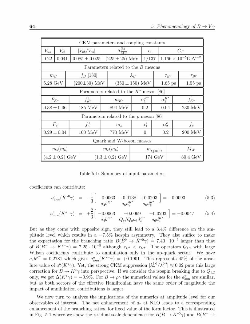
64 5. Phenomenology of B → V γ
CKM parameters and coupling constants
Vus Vcb |Vub/Vcb| Λ(5)
MSα GF
0.22 0.041 0.085± 0.025 (225± 25) MeV 1/137 1.166× 10⁻⁵GeV−2
Parameters related to the B mesons
mB fB [130] λB τB+ τB0
5.28 GeV (200±30) MeV (350± 150) MeV 1.65 ps 1.55 ps
Parameters related to the K∗ meson [86]
FK∗ f⊥K∗ mK∗ αK∗
1 αK∗
2 fK∗
0.38± 0.06 185 MeV 894 MeV 0.2 0.04 230 MeV
Parameters related to the ρ meson [86]
Fρ f⊥ρ mρ αρ
1 αρ2 fρ
0.29± 0.04 160 MeV 770 MeV 0 0.2 200 MeV
Quark and W-boson masses
mb(mb) mc(mb) mt,pole MW
(4.2± 0.2) GeV (1.3± 0.2) GeV 174 GeV 80.4 GeV
Table 5.1: Summary of input parameters.
coefficients can contribute:
acann(K∗0γ) = −1
3
[
−0.0063 +0.0138 +0.0203a4b
K∗
a6dK∗
v a6dK∗
v
]
= −0.0093 (5.3)
acann(K∗−γ) = +
2
3
[
−0.0063 −0.0069 +0.0203a4b
K∗
Qs/Qua6dK∗
v a6dK∗
v
]
= +0.0047 (5.4)
But as they come with opposite sign, they still lead to a 3.4% difference on the am-plitude level which results in a −7.5% isospin asymmetry. They also suffice to makethe expectation for the branching ratio B(B0 → K∗0γ) = 7.40 · 10−5 larger than thatof B(B− → K∗−γ) = 7.25 · 10−5 although τB0 < τB+ . The operators Q1,2 with largeWilson coefficients contribute to annihilation only in the up-quark sector. We havea1b
K∗
= 0.2781 which gives auann(K∗−γ) = +0.1901. This represents 45% of the abso-
lute value of au7(K∗γ). Yet, the strong CKM suppression |λ(s)u /λ
(s)c | ≈ 0.02 puts this large
correction for B → K∗γ into perspective. If we consider the isospin breaking due to Q1,2
only, we get ∆(K∗γ) = −0.9%. For B → ργ the numerical values for the apann are similar,but as both sectors of the effective Hamiltonian have the same order of magnitude theimpact of annihilation contributions is larger.
We now turn to analyze the implications of the numerics at amplitude level for ourobservables of interest. The net enhancement of a7 at NLO leads to a correspondingenhancement of the branching ratios, for fixed value of the form factor. This is illustratedin Fig. 5.1 where we show the residual scale dependence for B(B → K∗0γ) and B(B− →
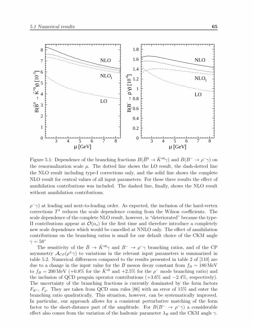
5.1 Numerical results 65
µ [GeV]
B(B−
0 → K−
*0γ)
[10-5
]
NLO
NLOI
LO
0
1
2
3
4
5
6
7
8
3 4 5 6 7 8µ [GeV]
B(B
- → ρ
- γ) [1
0-6]
NLO
NLOI
LO
0
0.2
0.4
0.6
0.8
1
1.2
1.4
1.6
1.8
3 4 5 6 7 8
Figure 5.1: Dependence of the branching fractions B(B0 → K∗0γ) and B(B− → ρ−γ) on
the renormalization scale µ. The dotted line shows the LO result, the dash-dotted line
the NLO result including type-I corrections only, and the solid line shows the complete
NLO result for central values of all input parameters. For these three results the effect of
annihilation contributions was included. The dashed line, finally, shows the NLO result
without annihilation contributions.
ρ−γ) at leading and next-to-leading order. As expected, the inclusion of the hard-vertexcorrections T I reduces the scale dependence coming from the Wilson coefficients. Thescale dependence of the complete NLO result, however, is “deteriorated” because the type-II contributions appear at O(αs) for the first time and therefore introduce a completelynew scale dependence which would be cancelled at NNLO only. The effect of annihilationcontributions on the branching ratios is small for our default choice of the CKM angleγ = 58◦
The sensitivity of the B → K∗0γ and B− → ρ−γ branching ratios, and of the CPasymmetry ACP (ρ
±γ) to variations in the relevant input parameters is summarized intable 5.2. Numerical differences compared to the results presented in table 2 of [110] aredue to a change in the input value for the B meson decay constant from fB = 180MeVto fB = 200MeV (+0.8% for the K∗0 and +2.5% for the ρ− mode branching ratio) andthe inclusion of QCD penguin operator contributions (+3.6% and −2.4%, respectively).The uncertainty of the branching fractions is currently dominated by the form factorsFK∗, Fρ. They are taken from QCD sum rules [86] with an error of 15% and enter thebranching ratio quadratically. This situation, however, can be systematically improved.In particular, our approach allows for a consistent perturbative matching of the formfactor to the short-distance part of the amplitude. For B(B− → ρ−γ) a considerableeffect also comes from the variation of the hadronic parameter λB and the CKM angle γ.
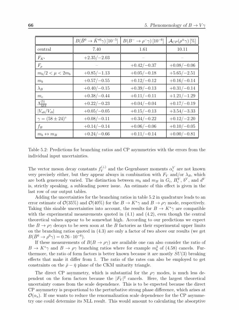
66 5. Phenomenology of B → V γ
B(B0 → K∗0γ) [10−5] B(B− → ρ−γ) [10−6] ACP (ρ±γ) [%]
central 7.40 1.61 10.11
FK∗ +2.35/−2.03 – –
Fρ – +0.42/−0.37 +0.08/−0.06
mb/2 < µ < 2mb +0.85/−1.13 +0.05/−0.18 +5.65/−2.51
mb +0.57/−0.55 +0.12/−0.12 +0.16/−0.14
λB +0.40/−0.15 +0.39/−0.13 +0.31/−0.14
mc +0.38/−0.44 +0.11/−0.11 +1.21/−1.29
Λ(5)
MS+0.22/−0.23 +0.04/−0.04 +0.17/−0.19
|Vub/Vcb| +0.05/−0.05 +0.15/−0.13 +3.54/−3.33
γ = (58± 24)◦ +0.08/−0.11 +0.34/−0.22 +0.12/−2.20
fB +0.14/−0.14 +0.06/−0.06 +0.10/−0.05
mb ↔ mB +0.24/−0.66 +0.11/−0.14 +0.00/−0.81
Table 5.2: Predictions for branching ratios and CP asymmetries with the errors from the
individual input uncertainties.
The vector meson decay constants f(⊥)V and the Gegenbauer moments αV
i are not knownvery precisely either, but they appear always in combination with FV and/or λB, whichare both generously varied. The distinction between mb and mB in Gi, H
Vi , b
V , and dV
is, strictly speaking, a subleading power issue. An estimate of this effect is given in thelast row of our output tables.
Adding the uncertainties for the branching ratios in table 5.2 in quadrature leads to anerror estimate of O(35%) and O(40%) for the B → K∗γ and B → ργ mode, respectively.Taking this sizable uncertainties into account, the results for B → K∗γ are compatiblewith the experimental measurements quoted in (4.1) and (4.2), even though the centraltheoretical values appear to be somewhat high. According to our predictions we expectthe B → ργ decays to be seen soon at the B factories as their experimental upper limitson the branching ratios quoted in (4.3) are only a factor of two above our results (we getB(B0 → ρ0γ) = 0.76 · 10−6).
If these measurements of B(B → ργ) are available one can also consider the ratio ofB → K∗γ and B → ργ branching ratios where for example m2
b of (4.58) cancels. Fur-thermore, the ratio of form factors is better known because it are mostly SU(3) breakingeffects that make it differ from 1. The ratio of the rates can also be employed to getconstraints on the ρ− η plane of the CKM unitarity triangle.
The direct CP asymmetry, which is substantial for the ργ modes, is much less de-pendent on the form factors because the |FV |2 cancels. Here, the largest theoreticaluncertainty comes from the scale dependence. This is to be expected because the directCP asymmetry is proportional to the perturbative strong phase difference, which arises atO(αs). If one wants to reduce the renormalization scale dependence for the CP asymme-try one could determine its NLL result. This would amount to calculating the absorptive
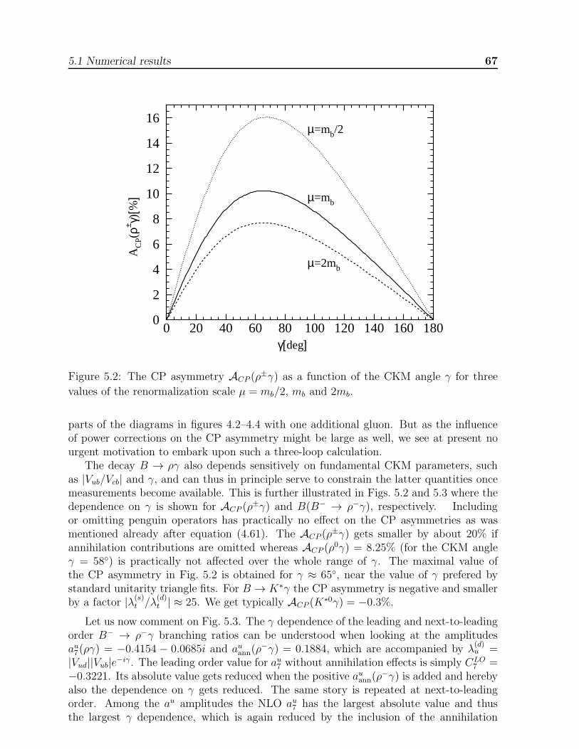
5.1 Numerical results 67
γ[deg]
AC
P(ρ± γ)
[%]
µ=mb/2
µ=mb
µ=2mb
0
2
4
6
8
10
12
14
16
0 20 40 60 80 100 120 140 160 180
Figure 5.2: The CP asymmetry ACP (ρ±γ) as a function of the CKM angle γ for three
values of the renormalization scale µ = mb/2, mb and 2mb.
parts of the diagrams in figures 4.2–4.4 with one additional gluon. But as the influenceof power corrections on the CP asymmetry might be large as well, we see at present nourgent motivation to embark upon such a three-loop calculation.
The decay B → ργ also depends sensitively on fundamental CKM parameters, suchas |Vub/Vcb| and γ, and can thus in principle serve to constrain the latter quantities oncemeasurements become available. This is further illustrated in Figs. 5.2 and 5.3 where thedependence on γ is shown for ACP (ρ
±γ) and B(B− → ρ−γ), respectively. Includingor omitting penguin operators has practically no effect on the CP asymmetries as wasmentioned already after equation (4.61). The ACP (ρ
±γ) gets smaller by about 20% ifannihilation contributions are omitted whereas ACP (ρ
0γ) = 8.25% (for the CKM angleγ = 58◦) is practically not affected over the whole range of γ. The maximal value ofthe CP asymmetry in Fig. 5.2 is obtained for γ ≈ 65◦, near the value of γ prefered bystandard unitarity triangle fits. For B → K∗γ the CP asymmetry is negative and smallerby a factor |λ(s)t /λ
(d)t | ≈ 25. We get typically ACP (K
∗0γ) = −0.3%.
Let us now comment on Fig. 5.3. The γ dependence of the leading and next-to-leadingorder B− → ρ−γ branching ratios can be understood when looking at the amplitudesau7(ργ) = −0.4154 − 0.0685i and auann(ρ
−γ) = 0.1884, which are accompanied by λ(d)u =
|Vud||Vub|e−iγ. The leading order value for au7 without annihilation effects is simply CLO7 =
−0.3221. Its absolute value gets reduced when the positive auann(ρ−γ) is added and hereby
also the dependence on γ gets reduced. The same story is repeated at next-to-leadingorder. Among the au amplitudes the NLO au7 has the largest absolute value and thusthe largest γ dependence, which is again reduced by the inclusion of the annihilation

68 5. Phenomenology of B → V γ
γ[deg]
B(B
- → ρ
- γ) [1
0-6]
NLO
NLOno ann
LO
LOno ann
0
0.5
1
1.5
2
2.5
3
3.5
4
4.5
0 20 40 60 80 100 120 140 160 180
Figure 5.3: The branching fraction B(B− → ρ−γ) as a function of the CKM angle γ at
leading and next-to-leading order with and without annihilation contributions.
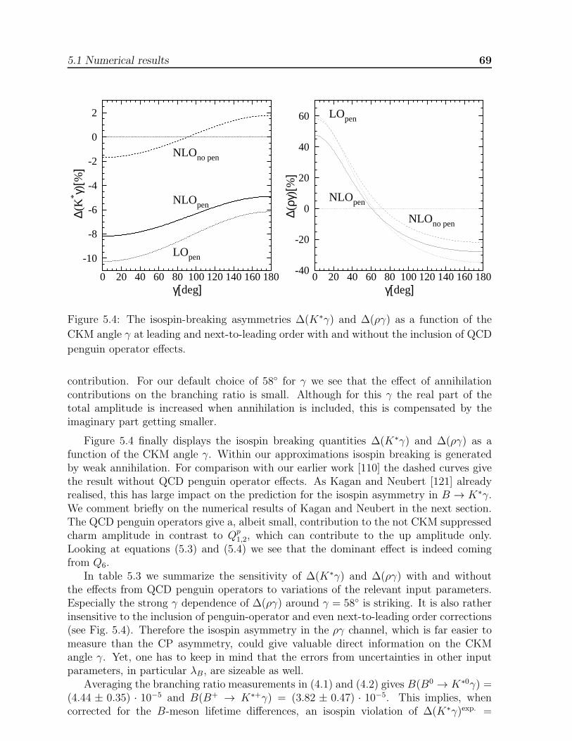
5.1 Numerical results 69
γ[deg]
∆(K
* γ)[%
]
NLOpen
LOpen
NLOno pen
-10
-8
-6
-4
-2
0
2
0 20 40 60 80 100 120 140 160 180γ[deg]
∆(ργ
)[%
]
NLOpen
LOpen
NLOno pen
-40
-20
0
20
40
60
0 20 40 60 80 100 120 140 160 180
Figure 5.4: The isospin-breaking asymmetries ∆(K∗γ) and ∆(ργ) as a function of the
CKM angle γ at leading and next-to-leading order with and without the inclusion of QCD
penguin operator effects.
contribution. For our default choice of 58◦ for γ we see that the effect of annihilationcontributions on the branching ratio is small. Although for this γ the real part of thetotal amplitude is increased when annihilation is included, this is compensated by theimaginary part getting smaller.
Figure 5.4 finally displays the isospin breaking quantities ∆(K∗γ) and ∆(ργ) as afunction of the CKM angle γ. Within our approximations isospin breaking is generatedby weak annihilation. For comparison with our earlier work [110] the dashed curves givethe result without QCD penguin operator effects. As Kagan and Neubert [121] alreadyrealised, this has large impact on the prediction for the isospin asymmetry in B → K∗γ.We comment briefly on the numerical results of Kagan and Neubert in the next section.The QCD penguin operators give a, albeit small, contribution to the not CKM suppressedcharm amplitude in contrast to Qp
1,2, which can contribute to the up amplitude only.Looking at equations (5.3) and (5.4) we see that the dominant effect is indeed comingfrom Q6.
In table 5.3 we summarize the sensitivity of ∆(K∗γ) and ∆(ργ) with and withoutthe effects from QCD penguin operators to variations of the relevant input parameters.Especially the strong γ dependence of ∆(ργ) around γ = 58◦ is striking. It is also ratherinsensitive to the inclusion of penguin-operator and even next-to-leading order corrections(see Fig. 5.4). Therefore the isospin asymmetry in the ργ channel, which is far easier tomeasure than the CP asymmetry, could give valuable direct information on the CKMangle γ. Yet, one has to keep in mind that the errors from uncertainties in other inputparameters, in particular λB, are sizeable as well.
Averaging the branching ratio measurements in (4.1) and (4.2) gives B(B0 → K∗0γ) =(4.44 ± 0.35) · 10−5 and B(B+ → K∗+γ) = (3.82 ± 0.47) · 10−5. This implies, whencorrected for the B-meson lifetime differences, an isospin violation of ∆(K∗γ)exp. =

70 5. Phenomenology of B → V γ
∆(K∗γ) [%] ∆no pen(K∗γ) [%] ∆(ργ) [%] ∆no pen(ρ
∗γ) [%]
central −7.46 −0.92 2.02 10.04
FK∗ +0.94/−1.26 +0.12/−0.16 – –
Fρ – – +1.23/−0.79 +2.54/−1.77
µ +2.69/−5.29 +0.05/−0.13 +2.41/−4.37 +1.89/−0.81
mb +0.46/−0.52 +0.04/−0.04 +0.01/−0.02 +0.60/−0.54
λB +1.71/−0.70 +0.27/−0.63 +15.56/−4.92 +13.65/−4.13
mc +0.20/−0.24 +0.03/−0.03 +0.19/−0.22 +0.03/−0.04
Λ(5)
MS+0.14/−0.13 +0.01/−0.01 +0.31/−0.28 +0.14/−0.12
|Vub/Vcb| +0.26/−0.26 +0.27/−0.27 +0.03/−1.62 +0.03/−1.76
γ = (58± 24)◦ +0.62/−0.46 +0.66/−0.49 +21.79/−14.10 +23.25/−15.04
fB +1.04/−1.01 +0.13/−0.13 +1.15/−0.96 +2.37/−2.17
mb ↔ mB +2.08/−1.72 +0.17/−0.22 +2.34/−0.29 +4.18/−2.45
Table 5.3: Predictions for the isospin-breaking asymmetries ∆(K∗γ) and ∆(ργ), including
and not including QCD-penguin-operator contributions, with the errors from the individ-
ual input uncertainties.
(−19.2 ± 11.8)%. It is not significantly different from zero and consistent with the value∆(K∗γ) = (−7.46+4.15
−5.89)% from table 5.3 when adding all uncertainties in quadrature. Ourcorresponding prediction for the ργ mode is ∆(ργ) = (2.02+27.01
−15.69)%.
The last application of our results we want to discuss is an estimate of U-spin breakingeffects in B → V γ decays. Using our expressions and central values for all parameterswe find for the differences of the charge conjugated branching ratios defined in (4.65) and(4.66)
∆B(B → K∗γ) = −7.3 · 10−7 (5.5)
∆B(B → ργ) = +4.3 · 10−7 (5.6)
where we have chosen the CKM angle γ = π/2 to maximise the effects. The two quantitiesindeed have opposite signs, but their sum only partly cancels, leaving a U-spin breakingremainder of −3.0 · 10−7 (for γ = 58◦ we get −2.6 · 10−7). This effect is almost entirelydue to the difference (FK∗ − Fρ). For form-factor values different from those in table 5.1the U-spin breaking effect would approximately be rescaled proportional to (FK∗ − Fρ).For our choice the U-spin breaking remainder is of the same order of magnitude as theindividual asymmetries. This example quantifies the limitations of the relation (4.67) asa Standard Model test.

5.2 Related Calculations 71
5.2 Related Calculations
Finally, we want to comment on related work done for B → V γ. Beneke, Feldmann,and Seidel treat exclusive B → V l+l− and B → V γ decays also in QCD factorization[118]. They use the CMM operator basis (2.58–2.65) supplemented with the semileptonicoperators P9 and P10
P9 =α
8π(ll)V (sb)V−A (5.7)
P10 =α
8π(ll)A(sb)V−A (5.8)
Another technical difference is that they use the formalism of [88] with our physical form
factor FK∗ replaced by its HQET analog ξ(K∗)⊥ . In this form factor the hard corrections
from diagrams as in Fig. 3.4 are taken explicitely into account. The analytic result of[118] for the B → K∗γ branching ratio perfectly agrees with ours. The numerical centralvalue is 8% larger because a somewhat larger value for the b quark mass was used. Theinterpretation is slightly different as well. Although within the error bars still consistentwith the experimental averages, Beneke, Feldmann, and Seidel get a little worried by thefact that the prediction for the central value of the branching ratio is nevertheless nearlytwice as large as the experimental central value. So they consider the possibility that theform factors at q2 = 0 are substantially different from what is obtained with QCD sumrules or in quark models. Fitting their result for the branching ratio to the experimentalvalue results in FK∗ = 0.27 ± 0.04, which is almost 30% smaller than the value we gavein table 5.1.
The paper of Kagan and Neubert [121] was mentioned already several times. Hereinthe leading isospin-breaking contributions to the B → K∗γ decay amplitudes are cal-culated. In particular a large effect from Q6 is obtained. This brings their theoreticalprediction in good agreement with the current experimental value. Yet, we have to keepin mind that there are still large error bars. The definition of the isospin-violating ratio
∆KN0− =
Γ(B0 → K∗0γ)− Γ(B− → K∗−γ)
Γ(B0 → K∗0γ) + Γ(B− → K∗−γ)(5.9)
Kagan and Neubert use differs by approximately a factor −1/2 from our ∆K∗
−0 in (4.63).In addition to the isospin-sensitive annihilation diagrams in Fig. 4.5 they also calcu-lated those penguin-annihilation and Q8 hard-spectator contributions of Fig. 4.6 wherethe photon is emitted from one of the upper light quark lines. As explained in section4.6 we included hereof only the annihilation contributions because they are numericallyenhanced, calculable, and not additionally suppressed by αs(O(mb)). With this choicewe get ∆KN
0− = (3.8+3.2−2.2)% for our input parameters. The main difference to the Kagan-
Neubert value of (8.0+2.1−3.2)% comes from other values of the form factor and B meson
decay constant used and from the different contributions included.In [116,117] the basic mechanisms for the B → V γ amplitudes at next-to-leading
order were already discussed. However, a simple model was used to take into account thebound-state effects. Additionally, some heuristic methods had to be used to regulate theinfrared divergences. These emerge from the quark self-energy diagrams and the b → sγvertex correction and are part of the form factor in our QCD factorization approach.The use of hadronic models does not allow a clear separation of short- and long-distancedynamics or a clean distinction of model-dependent and model-independent features.
72 5. Phenomenology of B → V γ
Another related work is that of Ali and Parkhomenko where also B → V γ is considered[119]. The first version of this work differed in some points from our results, but there isfull agreement after revision of the paper.
Last but not least we comment on a perturbative QCD study of the B → K∗γ decayby Li and Lin [131]. They calculate most of the relevant diagrams, in particular thespectator contribution from Q1. Yet, in our language, they include type-II correctionsonly, but thereof also power-suppressed contributions. The numerically much smallerresult for the branching ratio is used to determine the B meson wave function from a fitto the experimental data.

Part III
The Radiative Decays B → γγ


Chapter 6
The Basic Formulas for B → γγ
In the third part we discuss the double radiative B-meson decays Bs → γγ and Bd →γγ in QCD factorization. We systematically discuss the various contributions to theseexclusive processes in the heavy-quark limit mb ≫ ΛQCD. The factorization formula forthe hadronic matrix elements of local operators in the weak Hamiltonian again allowsus to separate perturbatively calculable hard scattering kernels from the nonperturbativeB-meson light-cone distribution amplitude. With power counting in ΛQCD/mb we identifyleading and subleading contributions to B → γγ. Only one diagram contributes at leadingpower, but an important class of subleading contributions can also be calculated. Theinclusion of these corrections is used to estimate CP asymmetries in B → γγ and one-particle irreducible two-photon emission from light-quark loops in B and D → γγ. Thesecorrections represent the quark-level analogue of so-called long-distance contributions tothese decays. In this chapter we give the basic formulas to leading logarithmic accuracyand discuss the leading-power and subleading-power contributions separately. Numericalresults are presented and discussed in chapter 7. Compared to our work in [132] we againinclude the QCD penguin operator contributions.
6.1 Motivation
For the double radiative decays B → γγ experimentally so far only upper limits on thebranching fractions exist:
B(B0s → γγ) < 1.48 · 10−4 at 90% C.L. [133]
B(B0d → γγ) < 1.7 · 10−6 at 90% C.L. [134]
(6.1)
The Standard Model expectations are roughly two orders of magnitude below these upperlimits. B → γγ decays have a rather clean experimental signature but are much bettersuited to be searched for at e+ e− B factories because at hadron colliders the combinatorialbackground is probably too large [135]. Furthermore these decays are of interest becausethey could provide useful tests of QCD dynamics in B decays. The B → γγ modesrealize the exceptional situation of nontrivial QCD dynamics related to the decaying B inconjunction with a completely nonhadronic final state and simple two-body kinematics.In principle they also probe the CKM parameters Vts and Vtd and could allow us to studyCP violating effects as the two-photon system can be in a CP-even or CP-odd state.

76 6. The Basic Formulas for B → γγ
The theoretical treatments of Bs → γγ performed so far [136–146] all had to employhadronic models to describe the Bs meson bound state dynamics. A clear separationof short- and long-distance dynamics and a distinction of model-dependent and model-independent features were therefore not possible. This concerns especially the dynamicsof the light-quark constituent inside the B, but also contributions from intermediate J/ψ,
ηc, φ, or D(∗)s meson states, which have been discussed as sources of potentially important
long-distance effects.
6.2 Basic Formulas
The effective Hamiltonian for b → sγγ is identical to the one for b → sγ transitions. Inaddition to the six four-quark operators Q1...6 in (2.50–2.55) or P1...6 in (2.58–2.63) thereare ten more gauge-invariant dimension-six operators with the right flavour quantumnumbers to contribute to a b → s transition. These are two-quark operators containingcombinations of the covariant derivative Dµ = ∂µ + ieQfAµ + igT aAa
µ, the photonic andgluonic field strength tensors, and their duals. Although these operators contain up tothree photon fields, Grinstein, Springer and Wise showed that the equations of motion[40]
i /Dq = mqq and DµFµν = eQq qγ
νq (6.2)
can be used to reduce them to the four-quark operator basis and the magnetic penguinoperators Q7 and Q8 [46]. Up to corrections of order 1/M2
W from higher-dimensionaloperators the effective Hamiltonian for b → sγγ thus is just the one of (2.48) for b →sγ. We use the standard operator basis (2.50–2.57). The most important operatorsare the magnetic penguin operator Q7 and the four-quark operators Qp
1,2. The effectiveHamiltonian for b→ dγγ is obtained from (2.48–2.57) by the replacement s→ d.
The amplitude for the B → γγ decay has the general structure
A(B → γ(k1, ǫ1)γ(k2, ǫ2)
)≡ GF√
2
α
3πfB
1
2〈γγ|A+FµνF
µν − i A−FµνFµν |0〉
=GF√2
α
3πfB[A+
(2k1 · ǫ2 k2 · ǫ1 −m2
Bǫ1 · ǫ2)− 2i A−ε(k1, k2, ǫ1, ǫ2)
](6.3)
Here F µν and F µν are the photon field strength tensor and its dual, where
F µν =1
2εµνλρFλρ (6.4)
with ε0123 = −1 again. The decay rate is then given by
Γ(B → γγ) =G2
Fm3Bf
2Bα
2
288π3
(|A+|2 + |A−|2
)(6.5)
In the heavy-quark limit we propose a factorization formula for the hadronic matrixelements of the operators in the effective Hamiltonian (2.48):
〈γ(ǫ1)γ(ǫ2)|Qi|B〉 =∫ 1
0
dξ T µνi (ξ) ΦB1(ξ)ǫ1µǫ2ν (6.6)

6.3 B → γγ at leading power 77
where the ǫi are the polarization 4-vectors of the photons and ΦB1 is the leading twistlight-cone distribution amplitude of the B meson defined in (3.19). If the light-like vectorn is chosen appropriately parallel to one of the 4-momenta of the photons only the firstnegative moment of ΦB1(ξ) appears, which we parametrize again via λB = O(ΛQCD) asin (3.21).
Because there are no hadrons in the final state only one type of hard-scattering kernelT (type II or hard-spectator contribution) enters the factorization formula. The QCDfactorization formula (6.6) holds up to corrections of relative order ΛQCD/mb. The formof (6.6) with a simple convolution over the light-cone variable ξ is appropriate for thelowest (leading logarithmic) order in αs, which we will use in the present analysis. Ageneralization to include transverse-momentum variables is likely to be necessary at higherorders in QCD [15,88,101,147].
We conclude this section with a brief discussion of CP violation in B → γγ. Thesubscripts ± on A±, defined in (6.3) for B → γγ, denote the CP properties of the corre-sponding two-photon final states, which are eigenstates of CP: ACP=+1 is proportional tothe parallel spin polarization ~ǫ1 ·~ǫ2 and ACP=−1 is proportional to the perpendicular spinpolarization ~ǫ1 × ~ǫ2 of the photons. In addition to A± we introduce the CP conjugatedamplitudes A± for the decay B → γγ (decaying b anti-quark). Then the deviation of theratios
r±CP =|A±|2 − |A±|2|A±|2 + |A±|2
(6.7)
from zero is a measure of direct CP violation. We shall focus here on this direct effect,which is specific for the B → γγ decay, and will not consider CP violation originating inB–B mixing.
Due to the unitarity of the CKM matrix we can parametrize
A± = λua±u e
iα±u + λca
±c e
iα±c (6.8)
A± = λ∗ua±u e
iα±u + λ∗ca
±c e
iα±c (6.9)
where a±u,c are real hadronic matrix elements of weak transition operators and the α±u,c are
their CP-conserving phases. We then have
r±CP =2 Im(λuλ
∗c)a
±u a
±c sin(α±
c − α±u )
|λu|2a±2u + |λc|2a±2
c + 2Re(λuλ∗c)a±u a
±c cos(α±
c − α±u )
(6.10)
The weak phase differences read
Im(λ(q)u λ(q)∗c ) = ∓|λ(q)u ||λ(q)c | sin γ (6.11)
with the negative sign for q = s and the positive sign for q = d. The strong phasedifferences sin(α±
c − α±u ) arise from final state interaction (FSI) effects, generated for
instance via the Bander-Silverman-Soni (BSS) mechanism [148].
6.3 B → γγ at leading power
To leading power in ΛQCD/mb and in the leading logarithmic approximation of QCD onlyone diagram contributes to the amplitude for B → γγ. It is the one-particle reducible

78 6. The Basic Formulas for B → γγ
b
s/d
Q7
Figure 6.1: The leading power contribution to the B → γγ amplitude given by the
magnetic penguin operator Q7. The diagram with interchanged photons is not shown.
Radiation from the b-quark line (Fig. 6.2) is power suppressed.
(1PR) diagram with the electromagnetic penguin operator Q7, where the second photonis emitted from the s-quark line. An illustration is given in Fig. 6.1. Evaluating thefactorization formula (6.6) for this diagram leads to the matrix element
〈γ(k1, ǫ1)γ(k2, ǫ2)|Q7|B〉 = (6.12)
ifBα
πQs
∫ 1
0
dξΦB1(ξ)
ξ
(2k1 · ǫ2k2 · ǫ1 −m2
Bǫ1 · ǫ2 − 2i ε(k1, k2, ǫ1, ǫ2))
Together with the effective Hamiltonian (2.48) and the definition of A± in (6.3) thisimplies
A± = λ(q)t C7
mB
λB(6.13)
where CKM unitarity, λ(q)u + λ
(q)c = −λ(q)t , has been used.
After summing over the photon polarizations the branching fraction to leading powerbecomes
B(Bq → γγ) = τBq
G2Fm
5Bq
192π3|λ(q)t |2C2
7
4α2f 2Bq
3λ2Bq
(6.14)
where q = d, s for the decay of a B0d or a B0
s meson, respectively.
In the present approximation the strong-interaction matrix elements multiplying λ(q)u
and λ(q)c are identical and have no relative phase. The CP-violating quantities r±CP defined
in (6.7) therefore vanish for the strictly leading-power result.
6.4 Power-suppressed contributions to B → γγ
Subleading contributions come from the 1PR diagram, where the second photon is emittedfrom the b quark line (Fig. 6.2), and from the one-particle irreducible diagram (1PI) (seeFig. 6.3).
To estimate the subleading 1PR contribution, we simply evaluate the graph in Fig. 6.2using the B-meson projector in (3.19). The result equals λB/mB times the leading-powerexpression in (6.12), clearly showing the power suppression of this mechanism. Othercorrections of the same order can arise from higher-twist terms in the B-meson wavefunction. We shall neglect all those subleading terms for the matrix element of Q7,

6.4 Power-suppressed contributions to B → γγ 79
b
s/dQ7
Figure 6.2: The subleading power 1PR diagram of the magnetic penguin operator Q7.
The diagram with interchanged photons is not shown.
b
s/d
Qi
Figure 6.3: The subleading power 1PI diagram. Here the four-quark operators Qi can
contribute. The diagram with interchanged photons is not shown.
keeping in mind that they could naturally contribute relative corrections of order ∼ 10%.We stress, however, that subleading effects in 〈Q7〉 contribute equally to the up- andcharm-quark components of the amplitude (see (2.48)). Therefore they do not give rise,in particular, to relative FSI phases between these sectors, which would affect direct CPviolation. The same is true for perturbative QCD corrections to 〈Q7〉.
We next consider more closely the diagrams in Fig. 6.3. These 1PI contributions,which come from the matrix elements of four-quark operators in (2.48), are of specialinterest for two reasons. First, they are the basic effects responsible for a difference be-tween the up- and charm-quark sectors of the amplitude, including rescattering phases.Second, they represent the parton-level processes that are dual to B → γγ amplitudesfrom Qi with hadronic intermediate states (J/Ψ, D(∗), etc.), which are commonly consid-ered as generic long-distance contributions. Investigating the amplitude in Fig. 6.3 couldtherefore shed light on this class of effects in B → γγ.
It shall now be argued that the 1PI contributions are calculable using QCD factoriza-tion. To this end we show at O(αs) that there are no collinear or soft infrared divergencesat leading power in 1/mb. By leading power we mean here the lowest nonvanishing orderin the power expansion, where the entire 1PI contribution starts only at subleading powerwith respect to the dominant mechanism in Fig. 6.1. This suppression will be apparentfrom the explicit expressions given in (6.18–6.23) below. The relevant diagrams at O(αs)are shown in Fig. 6.4. Following the approach explained in the second reference of [15]for the case of B → Dπ decays, we examine the potentially IR-singular regions of themomentum-space integrals in Fig. 6.4. We demonstrate the absence of divergences ortheir mutual cancellation among different diagrams for the hard-scattering part of theamplitude at O(αs). As a consequence the matrix elements of four-quark operators can

80 6. The Basic Formulas for B → γγ
(a)
s
tl
k1
k2
(b) (c)
(d) (e) (f)
Figure 6.4: The gluon corrections to the 1PI diagram. Quark labels are as in Fig. 6.3
and the momentum assignment is everywhere as in diagram (a). The diagrams with
interchanged photons are not shown.
be written in factorized form as in (6.6), where in the present case the kernel T µνi is
independent of ξ:〈γ(ǫ1)γ(ǫ2)|Q1...6|B〉 = fBT
µν1...6 ǫ1µǫ2ν (6.15)
Power counting shows that all diagrams in Fig. 6.4 are IR finite in the soft-soft andhard-soft region as well as when the gluon is collinear with one of the photon momentaand the quark in the loop is soft or supersoft. But for a soft or supersoft gluon emit-ted from the B meson spectator quark in addition to a collinear quark in the loop weencounter logarithmic IR-divergences. To leading power, however, setting the loop mo-mentum proportional to the photon momentum, the diagrams vanish individually. Thelast region of phase space we have to consider is where both the gluon momentum s andthe momentum of the quark in the loop t are collinear with one of the photon momenta,for example
s = αk2 + s⊥ t = βk2 + t⊥ (6.16)
where α, β ∼ 1 and s⊥, t⊥ ∼ ΛQCD ≪ mb. This again leads to a logarithmic IR divergence.The leading t = βk2 contribution vanishes again as in the (super)soft-collinear case.When the gluon is attached to the light spectator quark of the B meson and one ofthe two collinear quarks in the loop (Fig. 6.4 d,e), however, this contribution is powerenhanced by mb/ΛQCD compared to the hard diagram without any gluon (Fig. 6.3). Butfor factorization to hold, we need that the logarithmic divergences have coefficients thatare power suppressed. We therefore consider the next order in ΛQCD/mb by keeping thetransverse momentum of t and analyze these terms in more detail. It turns out that thecontributions from the loop where the gluon hits one of the collinear quarks are bothproportional to kα2 . The factor k
α2 is contracted with the open index of the gluon emission
from one of the B meson constituent quarks. Substituting s = αk2 and using pb and l forthe momenta of the b and the spectator quark in the B meson, respectively, we obtain

6.4 Power-suppressed contributions to B → γγ 81
for this term
s
[Γ( 6pb − α6k2 +mb)γα(pb − αk2)2 −m2
b
+γα(− 6 l + α6k2)Γ(−l + αk2)2
]
b kα2
= s
[Γ( 6pb − α6k2 +mb)( 6pb −mb)
α(pb − αk2)2 −m2b
+6 l(− 6 l + α6k2)Γ(−l + αk2)2
]
b
= 0 (6.17)
Here we employed the equations of motion for the constituent quarks of the B meson.It follows that the collinear-collinear divergences are also of sub-leading power. Thiscompletes our proof that at O(αs) for the 1PI contribution there are no collinear or softinfrared divergences at leading power in 1/mb in the hard-scattering kernel. It supportsour claim that these diagrams are calculable using QCD factorization. As no assumptionon the Dirac structure Γ of the inserted operator had to be made, this demonstrationapplies to all four-quark operators Q1...6 in any possible Fierz ordering.
For the evaluation of the 1PI diagram in Fig. 6.3 we can use the building blocksB
(V−A)×(V ∓A)αβ andB
(S+P )×(S−P )αβ of (4.20) and (4.23). We simply have to substitute gsT
a →Qqe, q → k1, r → k2, and can use the on-shell relations k2i = 0, ǫi · ki = 0 for bothphotons. Having regard to the possible insertions of the Fierz-transformed QCD penguinoperators, we find herewith the matrix elements
〈Qp1〉 = −fBqα
πQ2
ug(zp)ε(k1, k2, ǫ1, ǫ2) (6.18)
〈Qp2〉 = N〈Qp
1〉 (6.19)
〈Q3〉 = −fBqα
πε(k1, k2, ǫ1, ǫ2)
[
N∑
q
Q2qg(zq) +Q2
d(g(0) + g(1))
]
(6.20)
〈Q4〉 = −fBqα
πε(k1, k2, ǫ1, ǫ2)
[∑
q
Q2qg(zq) +NQ2
d(g(0) + g(1))
]
(6.21)
〈Q5〉 =fBqα
π
(
ε(k1, k2, ǫ1, ǫ2)
[
N∑
q
Q2qg(zq) +Q2
b(g(1) + 2)
]
(6.22)
−iQ2b
(
1− 3
2g(1)
)[
2k1 · ǫ2k2 · ǫ1 −m2Bqǫ1 · ǫ2
])
〈Q6〉 =fBqα
π
(
ε(k1, k2, ǫ1, ǫ2)
[∑
q
Q2qg(zq) +NQ2
b(g(1) + 2)
]
(6.23)
−iNQ2b
(
1− 3
2g(1)
)[
2k1 · ǫ2k2 · ǫ1 −m2Bqǫ1 · ǫ2
])
with
g(z) = −2 + 4z
[
L2
(2
1−√1− 4z + iǫ
)
+ L2
(2
1 +√1− 4z + iǫ
)]
(6.24)
Here the dilogarithmic function was defined already in (4.33), zq is again m2q/m
2b , and
p = u, c. We note that the function g(z) is related to the kernel h(u, z) defined in (4.32)in the context of B → V γ by g(z) = h(1, z). The function g(z) is regular for z → 0,

82 6. The Basic Formulas for B → γγ
g(0) = −2, and has an imaginary part growing almost linearly with z to sizeable valuesfor z = zc and vanishing again for z > 1/4. The imaginary part is due to the rescatteringprocess B → qq → γγ with an on-shell light-quark pair qq in the intermediate state. Sincethe process B → qq is forbidden by helicity and angular momentum conservation for amassless quark q, the function g(z) is real at z = 0 (that is for q = u, d, s). The helicitysuppression of the phase will be absent at higher order in αs.
Including the effect of 1PI diagrams in the decay amplitudes, the quantities A± from(6.13) become
Ap+ = −C7
mB
λB+ (C5 +NC6)
[1
2g(1)− 1
3
]
(6.25)
Ap− = −C7
mB
λB− 2
3(C1 +NC2) g(zp)− (C3 − C5)
[
2g(zc) +5
6g(1)
]
− (C4 − C6)
[2
3g(zc) +
7
6g(1)
]
+20
3C3 + 4C4 −
16
3C5 (6.26)
where we have decomposed A± into
A± =∑
p=u,c
λ(q)p Ap± (6.27)
neglected the light quark masses and used g(0) = −2. We see that the dominant effectis a modification of A− via the current-current operators Q1 and Q2. The imaginarypart of the 1PI loop diagram with a charm quark running in the loop leads to a relativeCP-conserving phase between the λu and the λc contribution. This gives a nonvanishingr−CP while r+CP is still zero because Au
+ = Ac+. The effect of QCD penguin operators is
small because of their tiny Wilson coefficients.
6.5 Long-distance contributions to B and D → γγ
Long-distance contributions were calculated for both B → γγ [141,142,149,150] and D →γγ [151,152]. Different mechanisms were considered:
• B and D → V γ followed by a V → γ conversion with the conversion factor suppliedby the vector meson dominance (VMD) model. This gives long-distance contri-butions to the operator Q7. Counting powers of mb in the explicit result for theBs → φγ → γγ amplitude in [141] shows that it is suppressed with ΛQCD/mb
compared to the leading power result from Fig. 6.1. Yet, it is just one among thesubleading power terms for the matrix element of Q7. Another comes for examplefrom the diagram in Fig. 6.2.
We can apply a similar power counting to the D → γγ VMD amplitude of [152].In the limit of a heavy charm quark it is likewise power suppressed with ΛQCD/mc
compared to the short-distance amplitude. The limit mc ≫ ΛQCD is certainly ques-tionable, but nevertheless some properties of charmed hadrons have been analyzedsuccessfully in this limit [153]. Again, the VMD contributions are just one out ofseveral possible power corrections to the Q7 matrix element.
6.5 Long-distance contributions to B and D → γγ 83
• Single-particle unitarity contributions where the D0 mixes with a spinless interme-diate particle, which decays into a photon pair. Such a process corresponds to our1PI contributions in Fig. 6.3. Relative to this contribution the amplitudes in [152]are at most of the same order in powers of the inverse “heavy” charm quark mass.
• Two-particle unitarity contributions are other hadron level counterparts of our 1PIdiagrams. Triangle loops with intermediate D
(∗)s [149,150] and K(∗) [152] mesons
were calculated for Bs → γγ and D → γγ, respectively. As we will see in the nextchapter, the effect of the 1PI contributions in B → γγ on the branching ratio is verysmall. The authors of [150] also get a not too large effect, reestimating the resultof [149]. Yet, one has to keep in mind that the effects from intermediate D and D∗
mesons are only two of many possible hadronic intermediate states.
With obvious replacements we can use our 1PI results in (6.18–6.23) to estimatethe quark-level analogue of the two-particle unitarity contributions to D → γγcalculated in [152]. For the current-current operators we get for the 1PI amplitude
AD→γγ1PI =
GF√2
α
πfDQ
2d (C1 +NC2) |Vcs||Vus|
[
g
(m2
s
m2c
)
− g(0)
]
i ε(ǫ1, ǫ2, k1, k2)
= −2.4 · 10−11GeV−1 [−0.2 + 0.5i± 0.1i] i ε(ǫ1, ǫ2, k1, k2)
|AD→γγ1PI | ≈ 1.3 · 10−11GeV−1ε(ǫ1, ǫ2, k1, k2) (6.28)
where we set fD = 200MeV and evaluated the Wilson coefficients at mc. Thecontributions of a strange quark and a down quark in the loop are accompanied byCKM elements which are practically equal in absolute value but opposite in sign.This leads to a strong GIM cancellation in the square bracket. If we neglected thestrange quark mass, the 1PI contribution would vanish altogether. This is a crucialdifference of the c → uγ transition at one loop compared to the b → sγ transitionand disturbs the hierarchy of higher order QCD terms. Leading logarithmic QCDcorrections are known to enhance the amplitude by more than an order of magnitude.Including the two-loop QCD contributions increases the amplitude further by twoorders of magnitude [154]. Therefore we would like to compare equation (6.28) withthe c → uγ amplitude from the dominant two-loop diagrams |A| = 0.0047 of [154].Evaluating the factorization formula then leads to the following “short distance”amplitude:
AD→γγSD = −GF√
2
α
πfDQuA
mD
λD
[2i ε(ǫ1, ǫ2, k1, k2)− 2k1 ·ǫ2 k2 ·ǫ1 +m2
Dǫ1 ·ǫ2]
|AD→γγSD,− | ≈ 12.8 · 10−11GeV−1ε(ǫ1, ǫ2, k1, k2) (6.29)
We see that the 1PI amplitude is smaller than the CP-odd part of the short distanceamplitude. This should be understood as an estimate only because we relied on theheavy quark limit for the charm quark.
Burdman, Golowich, Hewett, and Pakvasa on the other hand find a large effect ontheD → γγ branching ratio fromK+K− intermediate states [152]. Their amplitude,however, is formally suppressed with three powers relative to our 1PI amplitude. Inview of our above estimates the large effect could be overrated. Only one interme-diate state was taken into account so that important contributions in the duality

84 6. The Basic Formulas for B → γγ
sum might be missing. We also expect cancellations due to the GIM mechanism asexplicitely seen in our estimate above.
• The chain process Bs → φψ → φγ → γγ was estimated to give very small effectson the B → γγ decay amplitudes [142]. It is multiply power suppressed comparedto the leading power 1PR contribution.

Chapter 7
The Phenomenology of B → γγ
Here we present numerical results for the expressions derived in the previous chapter.Additionally to the input parameters given in table 5.1 we need the parameters relatedto the Bs meson. These we summarize in table 7.1. We will work to leading logarithmicorder in QCD and use the running mass mt(mt) = 166GeV for the top quark as input forthe Wilson coefficient C7. For definiteness we employ the two-loop form of the runningcoupling αs(µ) as quoted in (2.19), which corresponds to αs(MZ) = 0.118 for Λ
(5)
MS=
225MeV. With central values of all input parameters, at µ = mb, and using a nominalvalue of the CKM angle γ = 58◦ we find for the branching ratios to leading logarithmicaccuracy, evaluating (6.5), (6.25–6.27):
B(Bs → γγ) = 1.22 · 10−6 (7.1)
B(Bd → γγ) = 3.10 · 10−8 (7.2)
Using the leading power amplitudes (6.13) without the 1PI contributions we get
Bldg.pow.(Bs → γγ) = 1.17 · 10−6 (7.3)
Bldg.pow.(Bd → γγ) = 3.12 · 10−8 (7.4)
To display the size of power corrections from 1PI diagrams on amplitude level we compareAp
+ and Ap− in (6.25) and (6.26) with the leading power result Ap
±,ldg.pow. = −C7mBs/λBs
for Bs → γγ
Au/c+ = 4.872 +0.045 = 4.917
Au− = 4.872 +0.419 −0.061− 0.033 i = 5.230− 0.033 i
Ac− = 4.872 +0.203− 0.534 i −0.061− 0.033 i = 5.014− 0.567 i
ldg. pow. Q1,2 contribution Q3...6 contribution
(7.5)
Parameters related to the Bs meson
mBs fBs [130] τBs λBs
5.37 GeV (230 ± 30) MeV 1.49 ps (350± 150) MeV
Table 7.1: The input parameters for the Bs meson.
86 7. The Phenomenology of B → γγ
where we showed separately the leading power Q7 contribution and the effects fromcurrent-current and QCD-penguin operators to the 1PI contribution. For Bd → γγ nomi-nally only Ap
±,ldg.pow. = −C7mBs/λBs = 4.79 is changed. The calculable power correctionsthus are of the expected canonical size of O(10%). The precise value of these power-suppressed effects depends strongly on the renormalization scale µ. Typically, the relativesize of the 1PI terms diminishes when the scale is lowered, both due to an increase in C7
as well as the simultaneous decrease of the combination a2. The effect of QCD penguinoperators to the 1PI diagrams is small.
The main errors in (7.1–7.5) come from the variation of the nonperturbative inputparameters λB and the decay constants fBd
and fBs which are all poorly known andenter the branching ratios quadratically. The residual scale dependence is sizeable aswell because we calculated at leading logarithmic accuracy only. The variation of thebranching ratio with the scale would be less severe if next-to-leading QCD correctionswere known. We expect the NLL corrections to increase the branching ratio as was thecase for both the inclusive [41] and exclusive [110,118] b→ sγ decays.
The effect of next-to-leading logarithmic corrections for the branching ratio of b→ sγcan be reproduced by choosing a low renormalization scale (µ ≈ mb/2) in the leadinglogarithmic expressions. If such a low scale were also relevant for B → γγ the branchingratios would read
B(Bs → γγ)µ=mb/2 = 1.52 · 10−6 (7.6)
B(Bd → γγ)µ=mb/2 = 4.06 · 10−8 (7.7)
However, we prefer to use the nominal µ = mb and to quote the standard scale ambiguitywith mb/2 < µ < 2mb as a theoretical uncertainty.
For comparison we also show the results for the case where short-distance QCD effectsare neglected altogether. This amounts to taking µ = MW in the leading-order Wilsoncoefficients and leads to
B(Bs → γγ)µ=MW= 0.60 · 10−6 (7.8)
B(Bd → γγ)µ=MW= 1.22 · 10−8 (7.9)
Clearly, the leading logarithmic QCD corrections lead to a substantial enhancement ofthe branching ratios (7.1), (7.2), similar to the case of b → sγ.
The numerical evaluation of (6.10) gives for central values of the input parameters andat µ = mb the following predictions for the CP-violating ratios r−CP :
r−CP (Bs) = 0.35% (7.10)
r−CP (Bd) = −9.66% (7.11)
The effect is negligible for Bs → γγ as expected. For Bd → γγ CP violation occurs atthe level of about 10%. It is interesting to note that in B → γγ a non-vanishing CPasymmetry appears already at O(α0
s). This is possible via a modified BSS mechanism:Instead of the usual QCD penguin, already the electroweak loop in Fig. 6.3 itself leads to aCP-conserving phase. This phase difference defined in (6.10) is nonvanishing for the CP-odd amplitude only: α−
c − α−u = −6.1◦. Including the effects of QCD penguin operators
does not lead to a CP-conserving phase difference α+c − α+
u and therefore r+CP = 0.

87
γ[deg]
r CP- (B
q)[%
]
µ=mb/2
µ=mb
µ=2mb
rCP-(Bd)
rCP-(Bs)
-20
-17.5
-15
-12.5
-10
-7.5
-5
-2.5
0
2.5
5
0 20 40 60 80 100 120 140 160 180
Figure 7.1: The CP-violating ratios r−CP for decays of neutral Bd and Bs mesons to two
photons as a function of the CKM angle γ, each for three values of the renormalization
scale µ = mb/2, mb and 2mb.
The scale dependence of the CP asymmetry is rather strong, as can be seen in Fig. 7.1.The ratio rCP also depends sensitively on fundamental CKM parameters such as the CKMangle γ (Fig. 7.1). The extremal value of r−CP (Bd) is obtained for γ = 50◦. The sensitivityof the branching ratios and CP asymmetries to variations in the relevant input parametersis summarized in table 7.2.
Our predictions for the central values of the branching ratios are roughly two orders ofmagnitude below the current experimental bounds. The recent upper limit for B(Bd →γγ) from BaBar in (6.1) improved the previous limit from the L3 collaboration [155]by a factor of 20. With more integrated luminosity accumulated the upper bound willfurther be reduced. Yet, even with the planned total integrated luminosity of 500 fb−1
for each BaBar and BELLE, the number of Bd → γγ decays one expects to observe isonly a single one. The high-luminosity option SuperBaBar proposes to collect a totalintegrated luminosity of 10 ab−1. Therefore the number of observed events for Bd → γγwould be two dozens [156]. As long as the e+e− B factories run at the Υ(4s) resonancethey produce no Bs mesons and therefore cannot profit from the larger branching fractionto observe Bs → γγ decays. At hadron machines as the Fermilab Tevatron or the LHCat CERN all sorts of b-flavoured hadrons are produced. CDF, for instance, expects toobserve at the present run IIa at Tevatron in 2 fb−1 of data 28 million b→ J/ψX decays[13]. The number of Bs mesons will therefore be roughly 7 million. It will consequentlybe very hard to distinguish Bs → γγ events from the immense combinatorial backgroundevents.
As already mentioned, the dominant uncertainty for our prediction of the branching

88 7. The Phenomenology of B → γγ
B(Bd → γγ) B(Bs → γγ) r−CP (Bd) r−CP (Bs)
[10−8] [10−6] [%] [%]
central 3.09 1.22 −9.66 0.35
λB +6.40/−1.58 2.44/−0.61 +4.13/−4.02 +0.15/−0.15
fB +1.00/−0.86 +0.34/−0.30 – –
µ +0.97/−0.66 +0.31/−0.21 +9.03/−8.13 +0.30/−0.33
mc +0.10/−0.12 +0.03/−0.04 +1.79/−1.58 +0.06/−0.06
γ = (58± 24)◦ +1.28/−0.95 +0.01/−0.02 +1.66/−0.25 +0.06/−0.12
Table 7.2: Predictions for branching ratios and CP asymmetries with the errors from the
individual input uncertainties.
ratios comes from the variation of the hadronic parameter λB (factor 2). It governs theuncertainty of the leading power amplitude. So far, our value for λB quoted in table 5.1 isonly an educated guess with the uncertainty taken appropriately large. As λB enters theleading power branching ratio quadratically a large uncertainty in this input parameter istranslated into an even larger uncertainty of the branching ratio output. It would be highlydesirable to get a better understanding of λB. We hope that this problem can be attackedsoon with the help of QCD sum rule or lattice QCD techniques. As λB parametrizes thefirst negative moment of the B meson wave function it is a universal quantity and thereforeindependent of the precise decay under consideration. An extraction of it therefore mightbe possible from radiative semileptonic B decays, for instance.
Leaving the uncertainty of λB aside, the variation of the remaining parameters changesthe Bd → γγ and Bs → γγ branching ratios by order ±50% and ±35%, respectively. Ifboth the Bd → γγ and Bs → γγ branching ratios were measured one could consider theirratio where the dominant uncertainties from the λB and fB cancel to a large extent.
The main theoretical uncertainty for the CP asymmetries at present comes from thevariation of the renormalization scale µ. This could be reduced when QCD correctionsare included. But as the CP asymmetries in double radiative exclusive decays are ex-tremely hard to measure experimentally we see at present no urgent need to perform thiscalculation.

Part IV
Conclusions


Chapter 8
Conclusions
While waiting for the completion of LHC and new results from Tevatron Run II, B physicsis among the most active fields in recent particle physics. The main goal of B physics isa precision study of the flavour sector to extract Standard Model parameters with highprecision in order to reveal potential New Physics effects. Theoretically, the complicationis that three fundamental scales are involved in B decays: the weak interaction scale MW ,the b quark mass mb, and the QCD scale ΛQCD. Via the machinery of operator productexpansion and renormalization group equations in the framework of an effective theoryone can factorize perturbatively calculable short distance Wilson coefficients from the longdistance operator matrix elements. The latter pose the main difficulty as all low-energycontributions below the factorization scale µ = O(mb) are collected into them. Yet, onecan take advantage of the fact that mb ≫ ΛQCD and achieve a further separation of short-and long-distance part of these matrix elements. Employed for exclusive final states thisapplication of QCD factorization amounts to a systematic expansion in ΛQCD/mb and thestrong coupling parameter αs.
Within this thesis we have analyzed in detail the exclusive radiative decays B → V γ(V = K∗ or ρ) and B → γγ in QCD factorization. This enabled us to separate per-turbatively calculable contributions from the nonperturbative form factors and universalmeson light-cone distribution amplitudes. A power counting in ΛQCD/mb implies a hi-erarchy among the possible transition mechanisms and allows to identify leading andsubleading contributions.
Our framework has major advantages when compared with previous approaches toexclusive radiative decays. They all had to rely on hadronic models to estimate boundstate effects. These models, however, did not allow a clear separation of short- andlong-distance dynamics or a clean distinction of model-dependent and model-independentfeatures. QCD factorization is a systematic and model-independent approach based onfirst principles and the heavy-quark limit mb ≫ ΛQCD. It holds for mb → ∞. In real-ity, however, the bottom quark is not infinitely heavy so that we have to worry aboutΛQCD/mb power corrections. For the radiative B decays we considered, some of thesepower corrections - possibly the numerically most important ones - are calculable in QCDfactorization. The remaining ones are not expected to be very large. In particular, no“chirally enhanced” contributions, as in non-leptonic modes with pseudoscalar mesons inthe final state, can arise in our case.
Sizeable uncertainties come from the variation of the nonperturbative input parame-ters, in particular form factors, decay constants, and information on the B meson wave
92 8. Conclusions
function (λB), which are all poorly known. But we await progress on these quantitiesfrom lattice QCD and analytical methods as well as from an extraction from experimen-tal results.
An important conceptual aspect of our analyses is the interpretation of quark loopcontributions. We showed that these effects are calculable in QCD factorization. Before,such quark loops were considered as generic, uncalculable long-distance contributions.Non-factorizable long-distance corrections may still exist, but they are power-suppressed.Let us in the following address our findings for B → V γ and B → γγ separately.
The radiative decay with a vector meson K∗ in the final state is of particular promi-nence as its branching ratio was already measured. We presented in this work the firstreally complete calculation with next-to-leading logarithmic accuracy. Compared to ourpublication [110] we also included the effect of QCD penguin operators and added anexplicit proof, at one-loop order, for the factorizability of annihilation contributions. Atnext-to-leading order in QCD interesting effects occur: the operators Q1...6 and Q8 startcontributing, quark loops allow for CP-violating effects, and the hard-spectator correc-tions appear. We have seen that weak-annihilation amplitudes are power suppressed, butcalculable in QCD factorization and numerically important because they enter with largecoefficients. Therefore, we included their effects in our phenomenological discussion. Weestimated other power corrections to be numerically small.
Our NLO predictions for the central values of the branching ratios are
B(B0 → K∗0γ) = (7.4+2.6−2.4) · 10−5 B(B− → K∗−γ) = (7.3+2.6
−2.4) · 10−5
B(B0 → ρ0γ) = (0.8+0.4−0.3) · 10−6 B(B− → ρ−γ) = (1.6+0.7
−0.5) · 10−6
They are substantially larger than the leading logarithmic values when the same formfactors are used. The dominant correction comes from the hard-vertex contributions,which similarly increased the result for the inclusive B → Xsγ decay. Adding the effectof varying the input parameters in quadrature leads to an error estimate of O(35%) andO(40%) for the B → K∗γ and B → ργ branching ratios, respectively. For B(B → K∗γ)by far the dominant uncertainty comes from the B → K∗ form factor, which alone alreadyamounts to 30%. This situation, however, can be systematically improved. In particular,our approach allows for a consistent perturbative matching of the form factor to theshort-distance part of the amplitude. The largest uncertainty in B(B → ργ) is also theform factor. Yet, variation of the hadronic parameter λB and the CKM angle γ affect theprediction for the branching ratio also considerably.
Compared to the experimental measurements of the B → K∗γ branching ratios ourpredicted central values are somewhat high. Although within the uncertainties still com-patible, the discrepancy of the central values could be a hint that the form factors atq2 = 0 are smaller than the value obtained from QCD sum rules. At the present stage wealso cannot exclude that power corrections or even a failure of the QCD factorization ap-proach are responsible for the difference. Because the experimentally measured inclusiveb→ sγ rate is in good agreement with its theoretical prediction we do not expect sizeableNew Physics contributions to the exclusive B → K∗γ decays either. For the b → dγtransitions on the other hand there is still room for physics beyond the Standard Modelas experimentally at present only upper bounds for these decays exist. They are only afactor of two above our predictions so that we expect the B → ργ branching ratios tobe measured soon. From such a measurement we can obtain important information on

93
our input parameters, in particular the form factor, the hadronic parameter λB, and theCKM angle γ, and also on the validity of the QCD factorization approach to exclusiveradiative B decays.
For B → ργ both CKM sectors of the effective Hamiltonian have the same orderof magnitude. This allows a sizeable CP-violating asymmetry of A(ρ±γ) = 10.1%. In
B → K∗γ, on the other hand, |λ(s)u | ≪ |λ(s)c | and therefore the CP asymmetry is tiny,typically −0.5%. Because the CP asymmetry arises at O(αs) for the first time, we havea large dependence on the renormalization scale µ. This could be reduced by going oneorder further in perturbation theory, which would amount to a three-loop calculation.
We included the numerically most important power corrections - weak annihilation -into our analysis. Within our approximations weak annihilation is the only effect that issensitive to the charge of the B meson and therefore to isospin breaking. In B → K∗γannihilation contributions from Q1,2 are CKM suppressed such that their influence onthe branching ratio is small but a curiosity is a rather large effect of the QCD penguinoperator Q6 [121]. So for both B → K∗γ and B → ργ the isospin asymmetry is predictedto be sizeable: ∆(K∗γ) = (−7.5+4.1
−5.9)% and ∆(ργ) = (2.0+27.0−15.7)%. The isospin breaking in
B → ργ depends very sensitively on the CKM angle γ and can thus in principle serve toconstrain this quantity once measurements become available.
An explicit estimate of U-spin breaking effects in B → V γ decays quantified thelimitations of the use of U-spin symmetry in exclusive decays as a Standard Model test.
Our formalism can also straightforwardly be applied to other radiative rare B decays,such as Bs → V γ where V = φ, K∗, Bd → ωγ, or radiative decays to higher resonances.Some of these modes are discussed in [120,157]. Yet, for QCD factorization it is again theform factors, which pose the problem. To our knowledge they were never calculated. Thiswould be highly desireable because for example the B → K∗
2 (1430)γ decay was alreadyexperimentally observed [68,158].
The double radiative decays Bs → γγ and Bd → γγ were not seen in experimentyet. Within QCD factorization we predict the branching ratios to leading logarithmicaccuracy:
B(Bs → γγ) = (1.2+2.5−0.7) · 10−6
B(Bd → γγ) = (3.1+6.7−2.1) · 10−8
In the heavy quark limit the dominant contribution at leading power comes from only asingle diagram, but an important class of subleading contributions can also be calculated.We used these corrections to estimate CP asymmetries in B → γγ and one-particleirreducible two-photon emission from quark loops in D → γγ. The CP-violating ratior−CP (Bs) = 0.4% is negligible and r−CP (Bd) = −9.7%, albeit not very small, will not bemeasured in the near future.
The absolutely dominant uncertainty in the branching ratios comes from the variationof the hadronic parameter λB. This universal quantity is theoretically very poorly knownand enters the branching ratio quadratically. We propose to further investigate λB whichis of relevance also for other applications of QCD factorization to exclusive B mesondecays.
In table 8.1 we summarize the decay reach of the modes we discussed. The information

94 8. Conclusions
Hadron Collider e+e− B Factories
Experiments
Decay Branching CDF BTeV BaBar Super-
Mode Fractions D0 LHC-b Belle BaBar
(2 fb−1) (107 s) (0.5 ab−1) (10 ab−1)
B → K∗γ 5 · 10−5 170 25K 6K 120K
B → ργ 2 · 10−6 300 6K
B0d → γγ 3 · 10−8 1.3 25
Table 8.1: Decay reach of B experiments for exclusive radiative decays [156].
is taken from the Super-BaBar proposal [156]. Although in our estimate the branchingfraction for B0
d → γγ is by a factor of three larger compared to the value in [156], thesedecays are indeed very rare. The B0
s → γγ modes are roughly 40 times more frequent, butthey cannot be produced at the Υ(4s) resonance. At hadron colliders, on the other hand,also Bs mesons are produced. But the problem with the ργ and γγ final state in a hadroncollider environment is that the combinatorial background is extremely large. Photonsand ρ mesons are produced copiously. Therefore, in table 8.1 no estimates exist how manyof these decays could be really observed. Nevertheless we trust in the excellence of ourexperimental colleagues that they manage to measure the B → ργ or even B → γγ modesat hadron collider experiments. Running a prospective high-energy e+e− linear collideron the Z resonance could also improve the bounds on the B → γγ branching ratios oreven turn them into measurements.
According to Niels Bohr, the “goal of science is to gradually reduce our prejudice”[159]. We think we made one step in reducing the prejudice against a theoretical calcu-lation of exclusive decays. Many exclusive B decays can be treated successfully in QCDfactorization and the radiative ones are part of this set. QCD factorization has put thefear of God into hadronic matrix elements of exclusive B decays. Still a lot of work hasto be done, especially concerning the power corrections. But we have for the first timealso for exclusive decays a tool which is based on a systematic framework, namely theheavy-quark limit. We will see if the phenomenological impact of QCD factorization isequal.

Part V
Appendices

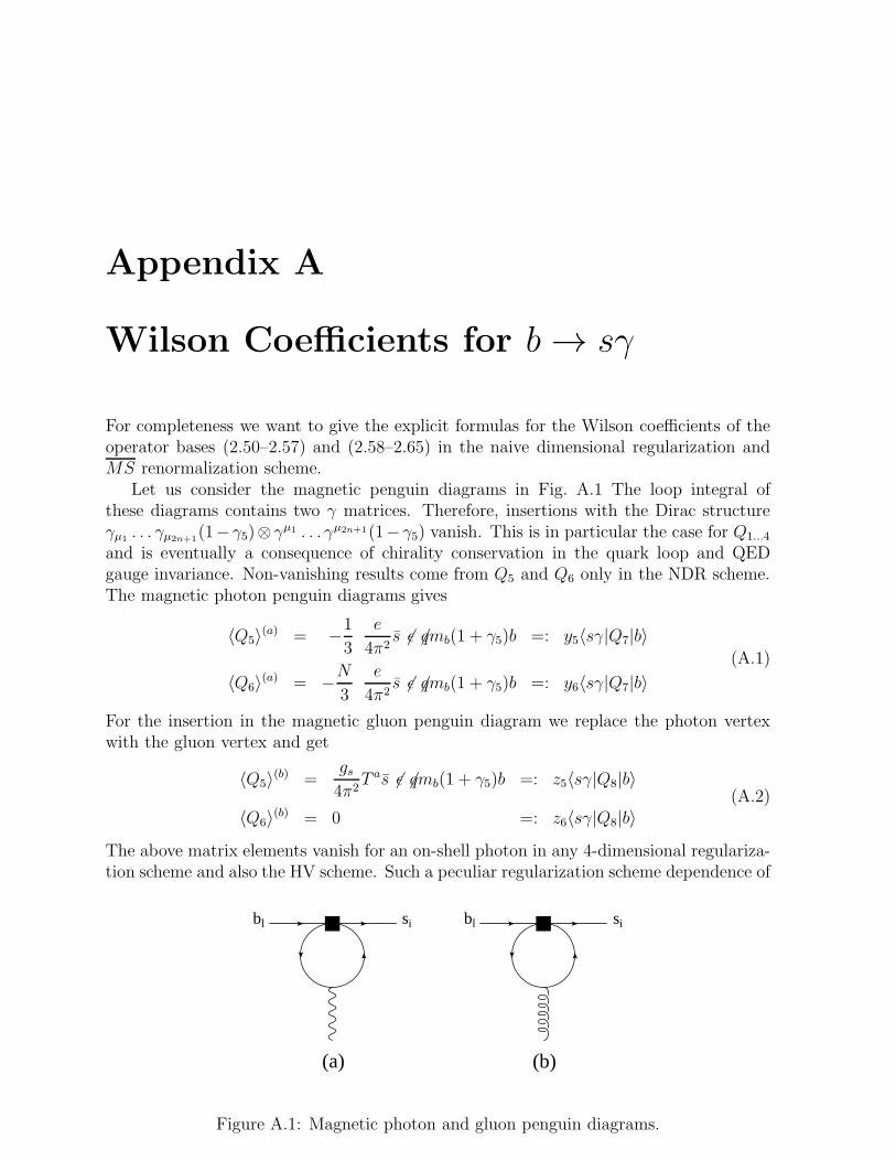
Appendix A
Wilson Coefficients for b→ sγ
For completeness we want to give the explicit formulas for the Wilson coefficients of theoperator bases (2.50–2.57) and (2.58–2.65) in the naive dimensional regularization andMS renormalization scheme.
Let us consider the magnetic penguin diagrams in Fig. A.1 The loop integral ofthese diagrams contains two γ matrices. Therefore, insertions with the Dirac structureγµ1 . . . γµ2n+1(1−γ5)⊗γµ1 . . . γµ2n+1(1−γ5) vanish. This is in particular the case for Q1...4
and is eventually a consequence of chirality conservation in the quark loop and QEDgauge invariance. Non-vanishing results come from Q5 and Q6 only in the NDR scheme.The magnetic photon penguin diagrams gives
〈Q5〉(a) = −1
3
e
4π2s 6ǫ 6qmb(1 + γ5)b =: y5〈sγ|Q7|b〉
〈Q6〉(a) = −N3
e
4π2s 6ǫ 6qmb(1 + γ5)b =: y6〈sγ|Q7|b〉
(A.1)
For the insertion in the magnetic gluon penguin diagram we replace the photon vertexwith the gluon vertex and get
〈Q5〉(b) =gs4π2
T as 6ǫ 6qmb(1 + γ5)b =: z5〈sγ|Q8|b〉
〈Q6〉(b) = 0 =: z6〈sγ|Q8|b〉(A.2)
The above matrix elements vanish for an on-shell photon in any 4-dimensional regulariza-tion scheme and also the HV scheme. Such a peculiar regularization scheme dependence of
bl si
(a)
bl si
(b)
Figure A.1: Magnetic photon and gluon penguin diagrams.
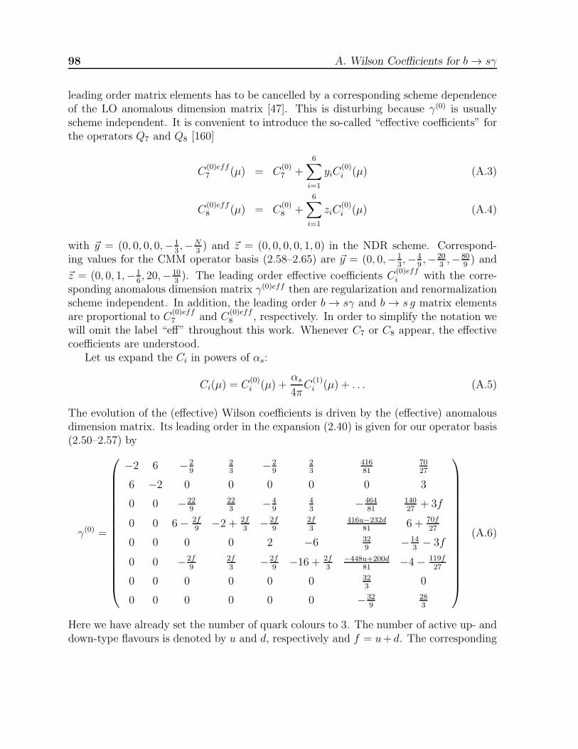
98 A. Wilson Coefficients for b→ sγ
leading order matrix elements has to be cancelled by a corresponding scheme dependenceof the LO anomalous dimension matrix [47]. This is disturbing because γ(0) is usuallyscheme independent. It is convenient to introduce the so-called “effective coefficients” forthe operators Q7 and Q8 [160]
C(0)eff7 (µ) = C
(0)7 +
6∑
i=1
yiC(0)i (µ) (A.3)
C(0)eff8 (µ) = C
(0)8 +
6∑
i=1
ziC(0)i (µ) (A.4)
with ~y = (0, 0, 0, 0,−13,−N
3) and ~z = (0, 0, 0, 0, 1, 0) in the NDR scheme. Correspond-
ing values for the CMM operator basis (2.58–2.65) are ~y = (0, 0,−13,−4
9,−20
3,−80
9) and
~z = (0, 0, 1,−16, 20,−10
3). The leading order effective coefficients C
(0)effi with the corre-
sponding anomalous dimension matrix γ(0)eff then are regularization and renormalizationscheme independent. In addition, the leading order b → sγ and b → s g matrix elementsare proportional to C
(0)eff7 and C
(0)eff8 , respectively. In order to simplify the notation we
will omit the label “eff” throughout this work. Whenever C7 or C8 appear, the effectivecoefficients are understood.
Let us expand the Ci in powers of αs:
Ci(µ) = C(0)i (µ) +
αs
4πC
(1)i (µ) + . . . (A.5)
The evolution of the (effective) Wilson coefficients is driven by the (effective) anomalousdimension matrix. Its leading order in the expansion (2.40) is given for our operator basis(2.50–2.57) by
γ(0) =
−2 6 −29
23
−29
23
41681
7027
6 −2 0 0 0 0 0 3
0 0 −229
223
−49
43
−46481
14027
+ 3f
0 0 6− 2f9
−2 + 2f3
−2f9
2f3
416u−232d81
6 + 70f27
0 0 0 0 2 −6 329
−143− 3f
0 0 −2f9
2f3
−2f9
−16 + 2f3
−448u+200d81
−4 − 119f27
0 0 0 0 0 0 323
0
0 0 0 0 0 0 −329
283
(A.6)
Here we have already set the number of quark colours to 3. The number of active up- anddown-type flavours is denoted by u and d, respectively and f = u+ d. The corresponding
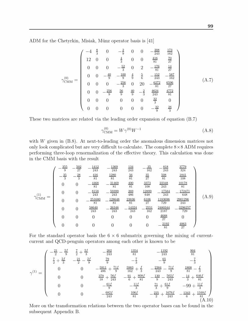
99
ADM for the Chetyrkin, Misiak, Munz operator basis is [41]
γ(0)CMM =
−4 83
0 −29
0 0 −208243
173162
12 0 0 43
0 0 41681
7027
0 0 0 −523
0 2 −17681
1427
0 0 −409
−1009
49
56
−152243
−587162
0 0 0 −2563
0 20 −627281
659627
0 0 −2569
569
409
−23
4624243
477281
0 0 0 0 0 0 323
0
0 0 0 0 0 0 −329
283
(A.7)
These two matrices are related via the leading order expansion of equation (B.7)
γ(0)CMM = Wγ(0)W−1 (A.8)
with W given in (B.8). At next-to-leading order the anomalous dimension matrices notonly look complicated but are very difficult to calculate. The complete 8×8 ADM requiresperforming three-loop renormalization of the effective theory. This calculation was donein the CMM basis with the result
γ(1)CMM =
−3559
−50227
−1412243
−1369243
134243
− 35162
−818243
3779324
−353
−283
−41681
128081
5681
3527
50881
1841108
0 0 −446881
−3146981
40081
3373108
22348243
1017881
0 0 −8158243
−59399243
269486
12899648
−17584243
−172471648
0 0 −25168081
−12864881
2383681
610627
1183696729
2901296243
0 0 58640243
−26348243
−14324243
−2551162
24803442187
−3296257729
0 0 0 0 0 0 468827
0
0 0 0 0 0 0 −219281
406327
(A.9)
For the standard operator basis the 6 × 6 submatrix governing the mixing of current-current and QCD-penguin operators among each other is known to be
γ(1) =
−212− 2f
972+ 2f
3−202
243135481
−1192243
90481
72+ 2f
3−21
2− 2f
9799
−73
−659
−73
0 0 −5911486
+ 71f9
5983162
+ f3
−2384243
− 71f9
180881
− f3
0 0 37918
+ 56f243
−916+ 808f
81−130
9− 502f
243−14
3+ 646f
81
0 0 −61f9
−11f3
713+ 61f
9−99 + 11f
3
0 0 −682f243
106f81
−2252
+ 1676f243
−13436
+ 1348f81
(A.10)More on the transformation relations between the two operator bases can be found in thesubsequent Appendix B.

100 A. Wilson Coefficients for b→ sγ
As explained in section 2.4, the initial conditions for the Wilson coefficients are foundby matching the effective theory amplitudes with the full Standard Model ones. Atµ0 =MW the leading-order results are
C(0)i (MW ) =
1 for i = 10 for i = 2 . . . 6
3x3t − 2x2t4(xt − 1)4
ln xt +−8x3t − 5x2t + 7xt
24(xt − 1)3for i = 7
−3x2t4(xt − 1)4
ln xt +−x3t + 5x2t + 2xt
8(xt − 1)3for i = 8
(A.11)
where
xi =m2
i
M2W
(A.12)
Up and charm quark mass are much smaller than the top quark mass and were thereforeneglected in (A.11). The only difference for the initial conditions in the CMM basis isthat the indices 1 and 2 are interchanged. Equating out (2.41) we get for our standardoperator basis
C(0)j (µ) =
8∑
i=1
kjiηai for j = 1 . . . 6 (A.13)
C(0)7 (µ) = η
1623C
(0)7 (MW ) +
8
3
(
η1423 − η
1623
)
C(0)8 (MW ) +
8∑
i=1
k7iηai (A.14)
C(0)8 (µ) = C(0)(MW )η
1423 +
8∑
i=1
k8iηai (A.15)
and
Z(0)j (µ) =
8∑
i=1
hjiηai for j = 1 . . . 6 (A.16)
Z(0)7 (µ) = C
(0)7 (µ) (A.17)
Z(0)8 (µ) = C
(0)8 (µ) (A.18)
for the CMM basis.At next-to-leading order we only need the Wilson coefficient C7. As explained in
Appendix B we have C(1)7 (µ) = Z
(1)7 (µ) and can directly take the formula from [41]
C(1)7 (µ) = η
3923C
(1)7 (MW ) +
8
3
(
η3723 − η
3923
)
C(1)8 (MW )
+
(297664
14283η
1623 − 7164416
357075η
1423 +
256868
14283η
3723 − 6698884
357075η
3923
)
C(0)8 (MW )
+37208
4761
(
η3923 − η
1623
)
C(0)7 (MW ) +
8∑
i=1
(eiηE(x) + fi + giη)ηai (A.19)
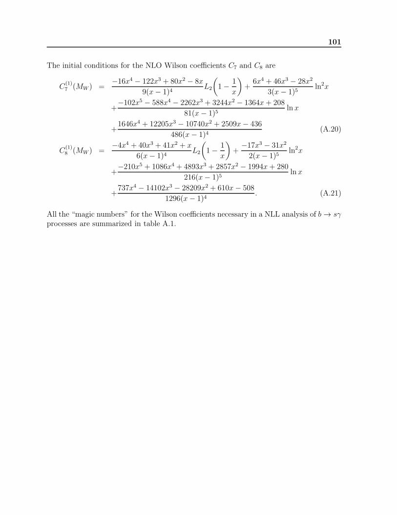
101
The initial conditions for the NLO Wilson coefficients C7 and C8 are
C(1)7 (MW ) =
−16x4 − 122x3 + 80x2 − 8x
9(x− 1)4L2
(
1− 1
x
)
+6x4 + 46x3 − 28x2
3(x− 1)5ln2x
+−102x5 − 588x4 − 2262x3 + 3244x2 − 1364x+ 208
81(x− 1)5ln x
+1646x4 + 12205x3 − 10740x2 + 2509x− 436
486(x− 1)4(A.20)
C(1)8 (MW ) =
−4x4 + 40x3 + 41x2 + x
6(x− 1)4L2
(
1− 1
x
)
+−17x3 − 31x2
2(x− 1)5ln2x
+−210x5 + 1086x4 + 4893x3 + 2857x2 − 1994x+ 280
216(x− 1)5ln x
+737x4 − 14102x3 − 28209x2 + 610x− 508
1296(x− 1)4. (A.21)
All the “magic numbers” for the Wilson coefficients necessary in a NLL analysis of b→ sγprocesses are summarized in table A.1.
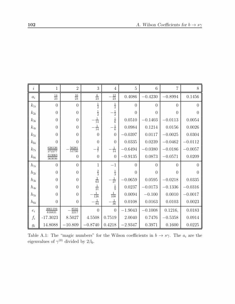
102 A. Wilson Coefficients for b→ sγ
i 1 2 3 4 5 6 7 8
ai1423
1623
623
−1223
0.4086 −0.4230 −0.8994 0.1456
k1i 0 0 12
12
0 0 0 0
k2i 0 0 12
−12
0 0 0 0
k3i 0 0 − 114
16
0.0510 −0.1403 −0.0113 0.0054
k4i 0 0 − 114
−16
0.0984 0.1214 0.0156 0.0026
k5i 0 0 0 0 −0.0397 0.0117 −0.0025 0.0304
k6i 0 0 0 0 0.0335 0.0239 −0.0462 −0.0112
k7i626126272277
−5628151730
−37
− 114
−0.6494 −0.0380 −0.0186 −0.0057
k8i313063363036
0 0 0 −0.9135 0.0873 −0.0571 0.0209
h1i 0 0 1 −1 0 0 0 0
h2i 0 0 23
13
0 0 0 0
h3i 0 0 263
− 127
−0.0659 0.0595 −0.0218 0.0335
h4i 0 0 121
19
0.0237 −0.0173 −0.1336 −0.0316
h5i 0 0 − 1126
1108
0.0094 −0.100 0.0010 −0.0017
h6i 0 0 − 184
− 136
0.0108 0.0163 0.0103 0.0023
ei4661194816831
−85162217
0 0 −1.9043 −0.1008 0.1216, 0.0183
fi -17.3023 8.5027 4.5508 0.7519 2.0040 0.7476 −0.5358 0.0914
gi 14.8088 −10.809 −0.8740 0.4218 −2.9347 0.3971 0.1600 0.0225
Table A.1: The “magic numbers” for the Wilson coefficients in b → sγ. The ai are the
eigenvalues of γ(0) divided by 2β0.

Appendix B
Operator Basis Transformations
Here we address the transformation relations of the operator bases (2.50–2.57) and (2.58–
2.65). In general, if we change the operator basis from ~Q to ~P = W ~Q, to translate thescheme-dependent NLO quantities like the NLOWilson coefficients or the NLO anomalousdimension matrix, we need the finite parts of the one-gluon exchange corrections to theoperator matrix elements where the scheme dependence is manifest. If the one-loop matrixelements in the starting basis are
〈 ~Q〉 =(
1 +αs
4πr)
〈 ~Q〉(0) (B.1)
then the ones in the transformed basis can be written as
〈~P 〉 =(
1 +αs
4πr′)
〈~P 〉(0) (B.2)
= W(
1 +αs
4π∆r)
〈 ~Q〉+O(α2s) (B.3)
with∆r =W−1r′W − r (B.4)
Denoting the Wilson coefficients in the transformed basis with ~Z, we can derive thetransformation rules starting from the fact that the full amplitude has to be the same inboth bases
~CT 〈 ~Q〉 != ~ZT 〈~P 〉 (B.5)
which leads to~Z =
(W−1
)T(
1− αs
4π∆rT
)
~C +O(α2s) (B.6)
For the sake of completeness we also give the transformation rule for the anomalousdimension matrix γ′ in the new basis which can be derived for example via differentiationof the left and right hand side of (B.6) with respect to lnµ using the definition of theanomalous dimension matrix in (2.38).
γ′ =W
{
γ +αs
4π[∆r, γ] + 2β0
(αs
4π
)2
∆r
}
W−1 +O(α3s) (B.7)
Here β0 was defined in (2.16) and the square brackets denote the commutator ∆r γ−γ∆r.The operator basis (2.50–2.57) we use mostly is apart from an overall factor of 4 and
the fact that we reversed the numbering of the current-current operators Q1,2 the same

104 B. Operator Basis Transformations
as the one of Greub, Hurth, and Wyler [60]. Chetyrkin, Misiak, and Munz [41] and alsoBuras, Czarnecki, Misiak, and Urban [61,62], however, use another operator basis (2.58–2.65), which is better suited for multi-loop calculations. The transformation matrix W infour space-time dimensions is given by
W =1
4
1 0 0 0 0 0 0 0−1
612
0 0 0 0 0 00 0 1 0 1 0 0 00 0 −1
612
−16
12
0 00 0 16 0 4 0 0 00 0 −8
38 −2
32 0 0
0 0 0 0 0 0 1 00 0 0 0 0 0 0 1
(B.8)
and transforms our operator basis (2.50–2.57) into the CMM basis (2.58–2.65)
PiD=4=
8∑
k=1
WikQk (B.9)
Note the block diagonal structure of W . The most important consequence hereof is thatW−1 as well has block diagonal form with the inverse of the submatrices as entries.
To determine ∆r we have to insert all the operators into current-current and penguindiagrams with one additional gluon. For the 6×6 submatrix of ∆r concerning the current-current and QCD penguin operators we calculated the diagrams (b), (c), (d), and (e) inFig. 2.5 with insertions of Q1...6 and P1...6. We get for N = 3
∆r6×6 =
12827
529
− 781
727
− 781
727
−231181
−17327
35243
−3581
35243
−3581
0 0 17827
−349
−16427
209
0 0 1− f9
−25+f3
−18−f9
6 + f3
0 0 −16027
169
14627
−29
0 0 −2 + f9
6− f3
3 + f9
−11−f3
(B.10)
which indeed transforms the NLO anomalous dimension matrix for our operator basis(A.10) into the 6×6 submatrix of (A.9). Without calculation we already can say that thefirst six entries of the seventh and eighth row of ∆r vanish because of the block diagonalstructure of W and W−1 and the fact that the magnetic penguin operators do not mixinto the four-quark operators. Yet, determining the entries in the seventh and eighthcolumns of r and r′ would amount to calculating the finite parts of the O(αs) virtualcorrections to the matrix elements for b → sγ. This challenging two-loop calculation iswhat Greub, Hurth, and Wyler [60] did for Q1,2 and Q7,8 of our operator basis. RecentlyBuras, Czarnecki, Misiak, and Urban performed this calculation for the complete CMMbasis (2.58–2.65) [61,62]. But the NLO matrix elements of the penguin operators in ouroperator basis have not yet been calculated so that we cannot determine the complete ∆r.Therefore we lack the information to translate the results of [61,62] into our operator basis.The use of only one operator basis would perhaps be interesting from an esthetical point

105
of view, but it is not necessary. We use the two different operator bases for physicallydistinct processes in B → V γ, namely hard vertex and hard spectator corrections whichis perfectly alright if the corresponding Wilson coefficients are used. For the Wilsoncoefficient of the electromagnetic penguin operator we need the next-to-leading value,which was calculated in [41] in the CMM basis.
To get C7 and C8 no transformation is necessary because the electro- and chromo-magnetic penguin operators are the same in both bases. Furthermore Q7 and Q8 cannotbe expressed as linear combinations of Q1...6 or P1...6 and they also do not mix into theseoperators. Using eq. (B.5) we therefore can identify the coefficients of 〈Q7,8〉 and 〈P7,8〉to be the same. So we can directly use the NLO result for Z7 from [41] for our operatorbasis.
Chetyrkin, Misiak, and Munz use a different strategy to derive the transformationproperties between the 6× 6 submatrices of the NLO anomalous dimension matrices [42].They pass from one operator basis to the other by a series of subsequent redefinitions ofphysical and evanescent operators.

106 B. Operator Basis Transformations
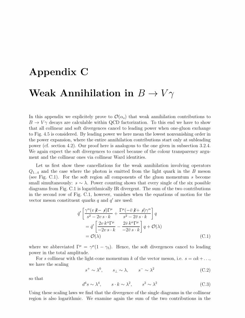
Appendix C
Weak Annihilation in B → V γ
In this appendix we explicitely prove to O(αs) that weak annihilation contributions toB → V γ decays are calculable within QCD factorization. To this end we have to showthat all collinear and soft divergences cancel to leading power when one-gluon exchangeto Fig. 4.5 is considered. By leading power we here mean the lowest nonvanishing order inthe power expansion, where the entire annihilation contributions start only at subleadingpower (cf. section 4.2). Our proof here is analogous to the one given in subsection 3.2.4.We again expect the soft divergences to cancel because of the colour transparency argu-ment and the collinear ones via collinear Ward identities.
Let us first show these cancellations for the weak annihilation involving operatorsQ1...4 and the case where the photon is emitted from the light quark in the B meson(see Fig. C.1). For the soft region all components of the gluon momentum s becomesmall simultaneously: s ∼ λ. Power counting shows that every single of the six possiblediagrams from Fig. C.1 is logarithmically IR divergent. The sum of the two contributionsin the second row of Fig. C.1, however, vanishes when the equations of motion for thevector meson constituent quarks q and q′ are used:
q′[γα(v 6k− 6s)Γµ
s2 − 2v s · k +Γµ(−v 6k+ 6s)γαs2 − 2v s · k
]
q
= q′[2v kαΓµ
−2v s · k − 2v kαΓµ
−2v s · k
]
q +O(λ)
= O(λ) (C.1)
where we abbreviated Γµ = γµ(1 − γ5). Hence, the soft divergences cancel to leadingpower in the total amplitude.
For s collinear with the light-cone momentum k of the vector meson, i.e. s = αk+ . . .,we have the scaling
s+ ∼ λ0, s⊥ ∼ λ, s− ∼ λ2 (C.2)
so thatd4s ∼ λ4, s · k ∼ λ2, s2 ∼ λ2 (C.3)
Using these scaling laws we find that the divergence of the single diagrams in the collinearregion is also logarithmic. We examine again the sum of the two contributions in the

108 C. Weak Annihilation in B → V γ
bQ1..4
s q
pb
l
s
vkvk
Figure C.1: One-gluon exchange corrections to the annihilation contribution to B → V γ
decay from Q1...4 operator insertions. The six possible diagrams are obtained through
combining the three diagrams in the first row with each of the two in the second row.
second row of Fig. C.1:
q′[γα(v − α) 6kΓµ
s2 − 2v s · k − Γµ(v − α) 6kγαs2 − 2v s · k
]
q
= q′[2(v − α)kαΓµ
s2 − 2v s · k − 2(v − α)kαΓµ
s2 − 2v s · k
]
q
∝ kα (C.4)
The kα is contracted with the γα from the gluon vertices in the first row of Fig. C.1
kα[
γα( 6 l − α 6k) 6ǫ( 6 l − α 6k− 6q)Γµ
(s2 − 2l · s)(s2 − 2l · s+ 2s · q − 2l · q) −6ǫ( 6 l− 6q)γα( 6 l− 6q − α 6k)Γµ
2l · q(s2 − 2l · s+ 2s · q − 2l · q)
+6ǫ( 6 l− 6q)Γµ( 6pb − α 6k +mb)γα
2l · q(s2 − 2pb · s)
]
(C.5)
The above expression vanishes when the equations of motion for the B meson quarks areused. So there are no collinear divergences at leading power either.
The other annihilation contribution which appears at the same level of power countingcomes from the insertion of operators Q5,6 and photon emission from one of the final statevector meson quarks. The one-gluon-exchange diagrams for the case where the photon isemitted from the antiquark in the vector meson are depicted in Fig. C.2. Both constituentquarks in the vector meson are light, collinear, and carry a momentum of the same size.Photon emission from the other vector meson quark therefore can be treated completelyanalogously.
A power counting as above shows that the two diagrams where the gluon hits theoff-shell light antiquark in the vector meson (third diagram in second row of Fig. C.2combined with the two diagrams in the first row) are infrared finite both in the soft andcollinear region. All other combinations are logarithmically divergent.
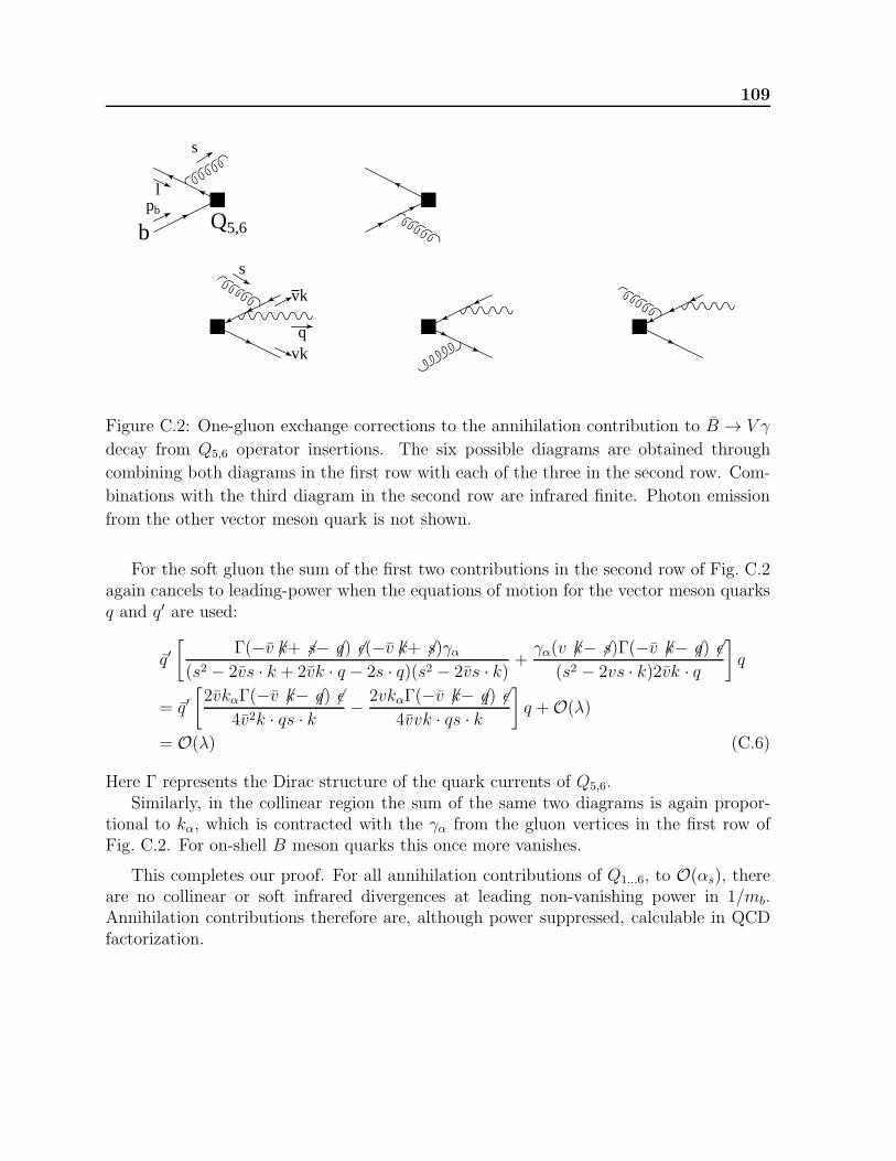
109
b Q5,6
s
pb
l
s
vk
vkq
Figure C.2: One-gluon exchange corrections to the annihilation contribution to B → V γ
decay from Q5,6 operator insertions. The six possible diagrams are obtained through
combining both diagrams in the first row with each of the three in the second row. Com-
binations with the third diagram in the second row are infrared finite. Photon emission
from the other vector meson quark is not shown.
For the soft gluon the sum of the first two contributions in the second row of Fig. C.2again cancels to leading-power when the equations of motion for the vector meson quarksq and q′ are used:
q′[
Γ(−v 6k+ 6s− 6q) 6ǫ(−v 6k+ 6s)γα(s2 − 2vs · k + 2vk · q − 2s · q)(s2 − 2vs · k) +
γα(v 6k− 6s)Γ(−v 6k− 6q) 6ǫ(s2 − 2vs · k)2vk · q
]
q
= q′[2vkαΓ(−v 6k− 6q) 6ǫ
4v2k · qs · k − 2vkαΓ(−v 6k− 6q) 6ǫ4vvk · qs · k
]
q +O(λ)
= O(λ) (C.6)
Here Γ represents the Dirac structure of the quark currents of Q5,6.Similarly, in the collinear region the sum of the same two diagrams is again propor-
tional to kα, which is contracted with the γα from the gluon vertices in the first row ofFig. C.2. For on-shell B meson quarks this once more vanishes.
This completes our proof. For all annihilation contributions of Q1...6, to O(αs), thereare no collinear or soft infrared divergences at leading non-vanishing power in 1/mb.Annihilation contributions therefore are, although power suppressed, calculable in QCDfactorization.

110 C. Weak Annihilation in B → V γ

Bibliography
[1] S. L. Glashow, “Partial Symmetries Of Weak Interactions,” Nucl. Phys. 22 (1961)579.
S. Weinberg, “A Model Of Leptons,” Phys. Rev. Lett. 19 (1967) 1264.
A. Salam, “Weak And Electromagnetic Interactions,” Originally printed in *N. Svart-holm: Elementary Particle Theory, Proceedings Of The Nobel Symposium Held 1968At Lerum, Sweden*, Stockholm 1968, 367-377.
[2] M. Gell-Mann, “A Schematic Model Of Baryons And Mesons,” Phys. Lett. 8 (1964)214.
M. Y. Han and Y. Nambu, “Three-Triplet Model With Double SU(3) Symmetry,”Phys. Rev. 139 (1965) B1006.
D. J. Gross and F. Wilczek, “Ultraviolet Behavior Of Nonabelian Gauge Theories,”Phys. Rev. Lett. 30 (1973) 1343.
H. D. Politzer, “Reliable Perturbative Results For Strong Interactions?,” Phys. Rev.Lett. 30 (1973) 1346.
S. Weinberg, “Nonabelian Gauge Theories Of The Strong Interactions,” Phys. Rev.Lett. 31 (1973) 494.
H. Fritzsch, M. Gell-Mann and H. Leutwyler, “Advantages Of The Color Octet GluonPicture,” Phys. Lett. B 47 (1973) 365.
[3] M. B. Green and J. H. Schwarz, “Anomaly Cancellation In Supersymmetric D = 10Gauge Theory And Superstring Theory,” Phys. Lett. B 149 (1984) 117.
E. Witten, “Dimensional Reduction Of Superstring Models,” Phys. Lett. B 155(1985) 151.
D. J. Gross, J. A. Harvey, E. J. Martinec and R. Rohm, “The Heterotic String,”Phys. Rev. Lett. 54 (1985) 502.
M. B. Green, J. H. Schwarz and E. Witten, “Superstring Theory.” Vol. 1: “In-troduction”, Cambridge, UK: Univ. Pr. (1987) 469 p. (Cambridge Monographs OnMathematical Physics); Vol. 2: “Loop Amplitudes, Anomalies And Phenomenology”,ibid. (1987) 596 p. (Cambridge Monographs On Mathematical Physics).
J. Polchinski, “String theory.” Vol. 1: “An introduction to the bosonic string,” Cam-bridge, UK: Univ. Pr. (1998) 402 p; Vol. 2: “Superstring theory and beyond,” Cam-bridge, UK: Univ. Pr. (1998) 531 p.
112 BIBLIOGRAPHY
[4] A. D. Sakharov, “Violation Of CP Invariance, C Asymmetry, And Baryon Asymme-try Of The Universe,” Pisma Zh. Eksp. Teor. Fiz. 5 (1967) 32 [JETP Lett. 5 (1967)24].
[5] J. H. Christenson, J. W. Cronin, V. L. Fitch and R. Turlay, “Evidence For The 2 πDecay Of The K0
2 Meson,” Phys. Rev. Lett. 13 (1964) 138.
[6] B. Aubert et al. [BABAR Collaboration], “Observation of CP violation in the B0
meson system,” Phys. Rev. Lett. 87 (2001) 091801.
K. Abe et al. [Belle Collaboration], “Observation of large CP violation in the neutralB meson system,” Phys. Rev. Lett. 87 (2001) 091802.
[7] S. W. Herb et al., “Observation Of A Dimuon Resonance At 9.5-GeV In 400-GeVProton - Nucleus Collisions,” Phys. Rev. Lett. 39 (1977) 252.
[8] P. F. Harrison and H. R. Quinn [BABAR Collaboration], “The BaBar physics book:Physics at an asymmetric B factory,” SLAC-R-0504 Papers from Workshop onPhysics at an Asymmetric B Factory (BaBar Collaboration Meeting), Rome, Italy,11-14 Nov 1996, Princeton, NJ, 17-20 Mar 1997, Orsay, France, 16-19 Jun 1997and Pasadena, CA, 22-24 Sep 1997.
[9] S. Mori et al. [BELLE Collaboration], “The Belle detector,” Nucl. Instrum. Meth. A479 (2002) 117.
[10] Y. Kubota et al. [CLEO Collaboration], “The CLEO-II detector,” Nucl. Instrum.Meth. A 320 (1992) 66.
[11] D. Abbaneo et al. [ALEPH Collaboration], “Combined results on b-hadron produc-tion rates, lifetimes, oscillations and semileptonic decays,” arXiv:hep-ex/0009052.
[12] F. Abe et al. [CDF Collaboration], “The CDF Detector: An Overview,” Nucl. In-strum. Meth. A 271 (1988) 387.
S. Abachi et al. [D0 Collaboration], “The D0 Detector,” Nucl. Instrum. Meth. A 338(1994) 185.
[13] K. Anikeev et al., “B physics at the Tevatron: Run II and beyond,” arXiv:hep-ph/0201071.
[14] P. Ball et al., “B decays at the LHC,” arXiv:hep-ph/0003238.
[15] M. Beneke, G. Buchalla, M. Neubert and C. T. Sachrajda, “QCD factorization forB → ππ decays: Strong phases and CP violation in the heavy quark limit,” Phys.Rev. Lett. 83 (1999) 1914.
M. Beneke, G. Buchalla, M. Neubert and C. T. Sachrajda, “QCD factorization forexclusive, non-leptonic B meson decays: General arguments and the case of heavy-light final states,” Nucl. Phys. B 591 (2000) 313.
M. Beneke, G. Buchalla, M. Neubert and C. T. Sachrajda, “QCD factorization inB → πK, ππ decays and extraction of Wolfenstein parameters,” Nucl. Phys. B 606(2001) 245.

BIBLIOGRAPHY 113
[16] A selection of useful textbooks of quantum field and gauge field theory:
D. Bailin and A. Love, “Introduction To Gauge Field Theory,” Bristol, UK: Hilger(1986) 348 p. (Graduate Student Series In Physics).
T. P. Cheng and L. F. Li, “Gauge Theory Of Elementary Particle Physics,” Oxford,UK: Clarendon (1984) 536 p. (Oxford Science Publications).
F. Halzen and A. D. Martin, “Quarks And Leptons: An Introductory Course InModern Particle Physics,” New York, Usa: Wiley (1984) 396p.
C. Itzykson and J. B. Zuber, “Quantum Field Theory,” New York, Usa: Mcgraw-hill(1980) 705 p.(International Series In Pure and Applied Physics).
F. Mandl and G. Shaw, “Quantum Field Theory,” Chichester, UK: Wiley (1984) 354p. (A Wiley-interscience Publication).
T. Muta, “Foundations of quantum chromodynamics. Second edition,” World Sci.Lect. Notes Phys. 57 (1998) 1.
M. E. Peskin and D. V. Schroeder, “An Introduction to quantum field theory,” Read-ing, USA: Addison-Wesley (1995) 842 p.
L. H. Ryder, “Quantum Field Theory,” Cambridge, UK: Univ. Pr. (1985) 443p.
S. Weinberg, “The Quantum theory of fields.” Vol. 1: Foundations, Cambridge, UK:Univ. Pr. (1995) 609 p; Vol. 2: Modern applications, ibid. (1996) 489 p.
[17] Y. Fukuda et al. [Super-Kamiokande Collaboration], “Evidence for oscillation of at-mospheric neutrinos,” Phys. Rev. Lett. 81 (1998) 1562.
[18] Y. L. Dokshitzer, “QCD and hadron dynamics,” Phil. Trans. Roy. Soc. Lond. A 359(2001) 309.
[19] P. W. Higgs, “Broken Symmetries And The Masses Of Gauge Bosons,” Phys. Rev.Lett. 13 (1964) 508.
P. W. Higgs, “Broken Symmetries, Massless Particles And Gauge Fields,” Phys. Lett.12 (1964) 132.
[20] [LEP Higgs Working Group for Higgs boson searches Collaboration], “Search for thestandard model Higgs boson at LEP,” (preliminary results), arXiv:hep-ex/0107029.
[21] N. Cabibbo, “Unitary Symmetry And Leptonic Decays,” Phys. Rev. Lett. 10 (1963)531.
M. Kobayashi and T. Maskawa, “CP Violation In The Renormalizable Theory OfWeak Interaction,” Prog. Theor. Phys. 49 (1973) 652.
[22] S. L. Glashow, J. Iliopoulos and L. Maiani, “Weak Interactions With Lepton - HadronSymmetry,” Phys. Rev. D 2 (1970) 1285.
[23] L. Wolfenstein, “Parametrization Of The Kobayashi-Maskawa Matrix,” Phys. Rev.Lett. 51 (1983) 1945.
[24] A. J. Buras, M. E. Lautenbacher and G. Ostermaier, “Waiting for the top quarkmass, K+ → π+νν, B0
s -B0s mixing and CP asymmetries in B decays,” Phys. Rev. D
50 (1994) 3433.
114 BIBLIOGRAPHY
[25] C. Jarlskog, “Commutator Of The Quark Mass Matrices In The Standard Elec-troweak Model And A Measure Of Maximal CP Violation,” Phys. Rev. Lett. 55(1985) 1039.
C. Jarlskog, “A Basis Independent Formulation Of The Connection Between QuarkMass Matrices, CP Violation And Experiment,” Z. Phys. C 29 (1985) 491.
[26] A. Hocker, H. Lacker, S. Laplace and F. Le Diberder, “A new approach to a globalfit of the CKM matrix,” Eur. Phys. J. C 21 (2001) 225.
The CKM Fitter homepage: http://ckmfitter.in2p3.fr/
[27] M. Ciuchini et al., “2000 CKM-triangle analysis: A critical review with updatedexperimental inputs and theoretical parameters,” JHEP 0107 (2001) 013.
[28] G. ’t Hooft and M. J. Veltman, “Regularization And Renormalization Of GaugeFields,” Nucl. Phys. B 44 (1972) 189.
[29] C. G. Bollini and J. J. Giambiagi, “Dimensional Renormalization: The Number OfDimensions As A Regularizing Parameter,” Nuovo Cim. B 12 (1972) 20.
J. F. Ashmore, “A Method Of Gauge Invariant Regularization,” Lett. Nuovo Cim. 4(1972) 289.
G. M. Cicuta and E. Montaldi, “Analytic Renormalization Via Continuous SpaceDimension,” Lett. Nuovo Cim. 4 (1972) 329.
[30] M. S. Chanowitz, M. Furman and I. Hinchliffe, “The Axial Current In DimensionalRegularization,” Nucl. Phys. B 159 (1979) 225.
[31] P. Breitenlohner and D. Maison, “Dimensional Renormalization And The ActionPrinciple,” Commun. Math. Phys. 52 (1977) 11.
P. Breitenlohner and D. Maison, “Dimensionally Renormalized Green’s FunctionsFor Theories With Massless Particles,” Commun. Math. Phys. 52 (1977) 39 and 55.
[32] A. J. Buras and P. H. Weisz, “QCD Nonleading Corrections To Weak Decays InDimensional Regularization And ’t Hooft-Veltman Schemes,” Nucl. Phys. B 333(1990) 66.
[33] G. ’t Hooft, “Renormalization Of Massless Yang-Mills Fields,” Nucl. Phys. B 33(1971) 173.
G. ’t Hooft, “Renormalizable Lagrangians For Massive Yang-Mills Fields,” Nucl.Phys. B 35 (1971) 167.
[34] G. ’t Hooft, “Dimensional Regularization And The Renormalization Group,” Nucl.Phys. B 61 (1973) 455.
[35] W. A. Bardeen, A. J. Buras, D. W. Duke and T. Muta, “Deep Inelastic ScatteringBeyond The Leading Order In Asymptotically Free Gauge Theories,” Phys. Rev. D18 (1978) 3998.
BIBLIOGRAPHY 115
[36] K. G. Wilson, “Nonlagrangian Models Of Current Algebra,” Phys. Rev. 179 (1969)1499.
K. G. Wilson and W. Zimmermann, “Operator Product Expansions and CompositeField Operators in the General Framework of Quantum Field Theory,” Commun.Math. Phys. 24 (1971) 87.
W. Zimmermann, “Normal Products And The Short Distance Expansion In ThePerturbation Theory Of Renormalizable Interactions,” Annals Phys. 77 (1973) 570[Lect. Notes Phys. 558 (1973) 278].
E. Witten, “Anomalous Cross-Section For Photon - Photon Scattering In GaugeTheories,” Nucl. Phys. B 120 (1977) 189.
[37] A. J. Buras, “Asymptotic Freedom In Deep Inelastic Processes In The Leading OrderAnd Beyond,” Rev. Mod. Phys. 52 (1980) 199.
[38] M. J. Dugan and B. Grinstein, “On the vanishing of evanescent operators,” Phys.Lett. B 256 (1991) 239.
[39] S. Herrlich and U. Nierste, “Evanescent operators, scheme dependences and doubleinsertions,” Nucl. Phys. B 455 (1995) 39.
[40] H. D. Politzer, “Power Corrections At Short Distances,” Nucl. Phys. B 172 (1980)349.
[41] K. Chetyrkin, M. Misiak and M. Munz, “Weak radiative B-meson decay beyondleading logarithms,” Phys. Lett. B 400 (1997) 206 [Erratum-ibid. B 425 (1997) 414]
[42] K. Chetyrkin, M. Misiak and M. Munz, “|∆(F )| = 1 nonleptonic effective Hamilto-nian in a simpler scheme,” Nucl. Phys. B 520 (1998) 279.
[43] G. Buchalla, A. J. Buras and M. E. Lautenbacher, “Weak Decays Beyond LeadingLogarithms,” Rev. Mod. Phys. 68 (1996) 1125.
[44] T. Inami and C. S. Lim, “Effects Of Superheavy Quarks And Leptons In Low-EnergyWeak Processes KL → µµ, K+ → π+νν and K0 ↔ K0,” Prog. Theor. Phys. 65(1981) 297 [Erratum-ibid. 65 (1981) 1772].
[45] M. K. Gaillard and B. W. Lee, “∆I = 1/2 Rule For Nonleptonic Decays In Asymp-totically Free Field Theories,” Phys. Rev. Lett. 33 (1974) 108.
G. Altarelli and L. Maiani, “Octet Enhancement Of Nonleptonic Weak InteractionsIn Asymptotically Free Gauge Theories,” Phys. Lett. B 52 (1974) 351.
F. J. Gilman and M. B. Wise, “Effective Hamiltonian For ∆S = 1 Weak NonleptonicDecays In The Six Quark Model,” Phys. Rev. D 20 (1979) 2392.
B. Guberina and R. D. Peccei, “Quantum Chromodynamic Effects And CP ViolationIn The Kobayashi-Maskawa Model,” Nucl. Phys. B 163 (1980) 289.
[46] B. Grinstein, R. P. Springer and M. B. Wise, “Strong Interaction Effects In WeakRadiative B Meson Decay,” Nucl. Phys. B 339 (1990) 269.

116 BIBLIOGRAPHY
[47] M. Ciuchini, E. Franco, G. Martinelli, L. Reina and L. Silvestrini, “Scheme indepen-dence of the effective Hamiltonian for b → sγ and b → sg decays,” Phys. Lett. B316 (1993) 127.
M. Ciuchini, E. Franco, L. Reina and L. Silvestrini, “Leading order QCD correctionsto b → sγ and b → sg decays in three regularization schemes,” Nucl. Phys. B 421(1994) 41.
[48] M. Misiak, “The b → s e+e− and b → sγ decays with next-to-leading logarithmicQCD corrections,” Nucl. Phys. B 393 (1993) 23 [Erratum-ibid. B 439 (1993) 461].
G. Cella, G. Curci, G. Ricciardi and A. Vicere, “The b → sγ decay revisited,” Phys.Lett. B 325 (1994) 227.
G. Cella, G. Curci, G. Ricciardi and A. Vicere, “QCD corrections to electroweakprocesses in an unconventional scheme: Application to the b → sγ decay,” Nucl.Phys. B 431 (1994) 417.
[49] S. Bertolini, F. Borzumati and A. Masiero, “QCD Enhancement Of Radiative BDecays,” Phys. Rev. Lett. 59 (1987) 180.
[50] N. G. Deshpande, P. Lo, J. Trampetic, G. Eilam and P. Singer, “B → K∗γ And TheTop Quark Mass,” Phys. Rev. Lett. 59 (1987) 183.
[51] R. Grigjanis, P. J. O’Donnell, M. Sutherland and H. Navelet, “QCD Corrected Effec-tive Lagrangian For b → s Processes,” Phys. Lett. B 213 (1988) 355 [Erratum-ibid.B 286 (1992) 413].
[52] G. Altarelli, G. Curci, G. Martinelli and S. Petrarca, “QCD Nonleading CorrectionsTo Weak Decays As An Application Of Regularization By Dimensional Reduction,”Nucl. Phys. B 187 (1981) 461.
[53] A. J. Buras, M. Jamin, E. Lautenbacher and P. H. Weisz, “Effective Hamiltoniansfor ∆S = 1 and ∆B = 1 nonleptonic decays beyond the leading logarithmic approx-imation,” Nucl. Phys. B 370 (1992) 69 [Addendum-ibid. B 375 (1992) 501].
[54] K. Adel and Y. P. Yao, “Exact αs calculation of b→ sγ and b→ sg,” Phys. Rev. D49 (1994) 4945
[55] C. Greub and T. Hurth, “Two-loop matching of the dipole operators for b→ sγ andb→ sg,” Phys. Rev. D 56 (1997) 2934.
A. J. Buras, A. Kwiatkowski and N. Pott, “Next-to-leading order matching for themagnetic photon penguin operator in the B → Xsγ decay,” Nucl. Phys. B 517 (1998)353.
[56] M. Ciuchini, G. Degrassi, P. Gambino and G. F. Giudice, “Next-to-leading QCDcorrections to B → Xsγ: Standard model and two-Higgs doublet model,” Nucl.Phys. B 527 (1998) 21.
[57] M. Ciuchini, E. Franco, G. Martinelli and L. Reina, “ǫ′/ǫ at the Next-to-leading orderin QCD and QED,” Phys. Lett. B 301 (1993) 263.

BIBLIOGRAPHY 117
M. Ciuchini, E. Franco, G. Martinelli and L. Reina, “The ∆S = 1 effective Hamilto-nian including next-to-leading order QCD and QED corrections,” Nucl. Phys. B 415(1994) 403,
[58] M. Misiak and M. Munz, “Two loop mixing of dimension five flavor changing oper-ators,” Phys. Lett. B 344 (1995) 308.
[59] M. A. Shifman and M. B. Voloshin, “Preasymptotic Effects In Inclusive Weak DecaysOf Charmed Particles,” Sov. J. Nucl. Phys. 41 (1985) 120. [Yad. Fiz. 41 (1985) 187].
J. Chay, H. Georgi and B. Grinstein, “Lepton Energy Distributions In Heavy MesonDecays From QCD,” Phys. Lett. B 247 (1990) 399.
I. I. Bigi, N. G. Uraltsev and A. I. Vainshtein, “Nonperturbative corrections to inclu-sive beauty and charm decays: QCD versus phenomenological models,” Phys. Lett.B 293 (1992) 430 [Erratum-ibid. B 297 (1992) 477].
[60] C. Greub, T. Hurth and D. Wyler, “Virtual corrections to the decay b→ sγ,” Phys.Lett. B 380 (1996) 385.
C. Greub, T. Hurth and D. Wyler, “Virtual O(αs) corrections to the inclusive decayb→ sγ,” Phys. Rev. D 54 (1996) 3350.
[61] A. J. Buras, A. Czarnecki, M. Misiak and J. Urban, “Two-loop matrix element ofthe current-current operator in the decay b→ Xsγ,” Nucl. Phys. B 611 (2001) 488.
[62] A. J. Buras, A. Czarnecki, M. Misiak and J. Urban, “Completing the NLO QCDcalculation of B → Xsγ,” Nucl. Phys. B 631 (2002) 219
[63] A. Ali and C. Greub, “Inclusive photon energy spectrum in rare B decays,” Z. Phys.C 49 (1991) 431.
A. Ali and C. Greub, “A Profile of the final states in B → Xsγ and an estimate ofthe branching ratio B(B → K∗γ),” Phys. Lett. B 259 (1991) 182.
A. Ali and C. Greub, “Photon energy spectrum in B → Xsγ and comparison withdata,” Phys. Lett. B 361 (1995) 146.
N. Pott, “Bremsstrahlung corrections to the decay b→ sγ,” Phys. Rev. D 54 (1996)938.
[64] A. Czarnecki and W. J. Marciano, “Electroweak radiative corrections to b → sγ,”Phys. Rev. Lett. 81 (1998) 277.
A. Strumia, “Two loop heavy top corrections to the b → sγ decay,” Nucl. Phys. B532 (1998) 28.
K. Baranowski and M. Misiak, “The O(αem/αs) correction to B(B → Xsγ),” Phys.Lett. B 483 (2000) 410.
P. Gambino and U. Haisch, “Electroweak effects in radiative B decays,” JHEP 0009(2000) 001.
P. Gambino and U. Haisch, “Complete electroweak matching for radiative B decays,”JHEP 0110 (2001) 020.

118 BIBLIOGRAPHY
[65] M. B. Voloshin, “Large O(1/m2c) nonperturbative correction to the inclusive rate of
the decay B → Xsγ,” Phys. Lett. B 397 (1997) 275.
[66] Z. Ligeti, L. Randall and M. B. Wise, “Comment on nonperturbative effects in B →Xsγ,” Phys. Lett. B 402 (1997) 178.
A. K. Grant, A. G. Morgan, S. Nussinov and R. D. Peccei, “Comment on nonper-turbative O(1/m2
c) corrections to Γ(B → Xsγ),” Phys. Rev. D 56 (1997) 3151.
[67] G. Buchalla, G. Isidori and S. J. Rey, “Corrections of order Λ2QCD/m
2c to inclusive
rare B decays,” Nucl. Phys. B 511 (1998) 594.
[68] S. Chen et al. [CLEO Collaboration], “Branching fraction and photon energy spec-trum for b → sγ,” Phys. Rev. Lett. 87 (2001) 251807.
[69] R. Barate et al. [ALEPH Collaboration], “A measurement of the inclusive b → sγbranching ratio,” Phys. Lett. B 429 (1998) 169.
[70] K. Abe et al. [Belle Collaboration], “A measurement of the branching fraction forthe inclusive B → Xsγ decays with Belle,” Phys. Lett. B 511, 151 (2001).
[71] P. Gambino and M. Misiak, “Quark mass effects in B → Xsγ,” Nucl. Phys. B 611(2001) 338.
[72] P. Krawczyk and S. Pokorski, “Constraints on CP violation by a nonminimal Higgssector from CP conserving processes,” Nucl. Phys. B 364 (1991) 10.
P. Ciafaloni, A. Romanino and A. Strumia, “Two-loop QCD corrections to charged-Higgs-mediated b→ sγ decay,” Nucl. Phys. B 524 (1998) 361.
F. M. Borzumati and C. Greub, “2HDMs predictions for B → Xsγ in NLO QCD,”Phys. Rev. D 58 (1998) 074004.
[73] L. Randall and R. Sundrum, “b → sγ and Bs → µ+µ− in extended technicolormodels,” Phys. Lett. B 312 (1993) 148.
[74] S. Bertolini, F. Borzumati, A. Masiero and G. Ridolfi, “Effects of supergravity in-duced electroweak breaking on rare B decays and mixings,” Nucl. Phys. B 353 (1991)591.
M. A. Diaz, “Constraints on supersymmetry due to b → sγ: An Improved calcula-tion,” Phys. Lett. B 304 (1993) 278.
R. Garisto and J. N. Ng, “Supersymmetric b→ sγ with large chargino contributions,”Phys. Lett. B 315 (1993) 372.
S. Bertolini and F. Vissani, “Supersymmetric predictions for the inclusive b → sγdecay,” Z. Phys. C 67 (1995) 513.
M. Ciuchini, G. Degrassi, P. Gambino and G. F. Giudice, “Next-to-leading QCDcorrections to B → Xsγ in supersymmetry,” Nucl. Phys. B 534 (1998) 3.
[75] J. D. Bjorken, “Topics In B Physics,” Nucl. Phys. Proc. Suppl. 11 (1989) 325.
[76] M. J. Dugan and B. Grinstein, “QCD basis for factorization in decays of heavymesons,” Phys. Lett. B 255 (1991) 583.

BIBLIOGRAPHY 119
[77] D. Fakirov and B. Stech, “F And D Decays,” Nucl. Phys. B 133 (1978) 315.
N. Cabibbo and L. Maiani, “Two Body Decays Of Charmed Mesons,” Phys. Lett. B73 (1978) 418 [Erratum-ibid. B 76 (1978) 663].
[78] M. Bauer and B. Stech, “Exclusive D Decays,” Phys. Lett. B 152 (1985) 380.
M. Bauer, B. Stech and M. Wirbel, “Exclusive Nonleptonic Decays Of D, Ds, AndB Mesons,” Z. Phys. C 34 (1987) 103.
[79] J. M. Soares, “Nonfactorizable terms in hadronic B meson weak decays,” Phys. Rev.D 51 (1995) 3518.
[80] M. Neubert and B. Stech, “Non-leptonic weak decays of B mesons,” Adv. Ser. Direct.High Energy Phys. 15 (1998) 294.
[81] H. Y. Cheng and B. Tseng, “Nonfactorizable effects in spectator and penguin ampli-tudes of hadronic charmless B decays,” Phys. Rev. D 58 (1998) 094005.
Y. H. Chen, H. Y. Cheng, B. Tseng and K. C. Yang, “Charmless hadronic two-bodydecays of Bu and Bd mesons,” Phys. Rev. D 60 (1999) 094014.
A. Ali and C. Greub, “An analysis of two-body non-leptonic B decays involving lightmesons in the standard model,” Phys. Rev. D 57 (1998) 2996.
A. Ali, G. Kramer and C. D. Lu, “Experimental tests of factorization in charmlessnon-leptonic two-body B decays,” Phys. Rev. D 58 (1998) 094009.
[82] A. J. Buras and L. Silvestrini, “Generalized factorization in non-leptonic two-bodyB decays: A critical look,” Nucl. Phys. B 548 (1999) 293.
[83] G. P. Lepage and S. J. Brodsky, “Exclusive Processes In Perturbative QuantumChromodynamics,” Phys. Rev. D 22 (1980) 2157.
A. V. Efremov and A. V. Radyushkin, “Factorization And Asymptotical BehaviorOf Pion Form-Factor In QCD,” Phys. Lett. B 94 (1980) 245.
[84] V. L. Chernyak and I. R. Zhitnitsky, “B Meson Exclusive Decays Into Baryons,”Nucl. Phys. B 345 (1990) 137.
[85] P. Ball and V. M. Braun, “The ρ Meson Light-Cone Distribution Amplitudes ofLeading Twist Revisited,” Phys. Rev. D 54 (1996) 2182.
[86] P. Ball and V. M. Braun, “Exclusive semileptonic and rare B meson decays in QCD,”Phys. Rev. D 58 (1998) 094016.
[87] A. G. Grozin and M. Neubert, “Asymptotics of heavy-meson form factors,” Phys.Rev. D 55 (1997) 272.
[88] M. Beneke and T. Feldmann, “Symmetry-breaking corrections to heavy-to-light Bmeson form factors at large recoil,” Nucl. Phys. B 592 (2001) 3.
[89] C. W. Bauer, D. Pirjol and I. W. Stewart, “A proof of factorization for B → Dπ,”Phys. Rev. Lett. 87 (2001) 201806.
C. W. Bauer, D. Pirjol and I. W. Stewart, “Soft-collinear factorization in effectivefield theory,” Phys. Rev. D 65 (2002) 054022.
120 BIBLIOGRAPHY
[90] A. Khodjamirian, “B → ππ decay in QCD,” Nucl. Phys. B 605 (2001) 558.
[91] M. Diehl and G. Hiller, “New ways to explore factorization in b decays,” JHEP 0106(2001) 067.
[92] G. ’t Hooft, “A Planar Diagram Theory For Strong Interactions,” Nucl. Phys. B 72(1974) 461.
G. ’t Hooft, “A Two-Dimensional Model For Mesons,” Nucl. Phys. B 75 (1974) 461.
E. Witten, “Baryons In The 1/N Expansion,” Nucl. Phys. B 160 (1979) 57.
[93] A. J. Buras, J. M. Gerard and R. Ruckl, “1/N Expansion For Exclusive And InclusiveCharm Decays,” Nucl. Phys. B 268 (1986) 16.
[94] W. A. Bardeen, A. J. Buras and J. M. Gerard, “The ∆I = 1/2 Rule In The LargeN Limit,” Phys. Lett. B 180 (1986) 133.
W. A. Bardeen, A. J. Buras and J. M. Gerard, “The K → ππ Decays In The LargeN Limit: Quark Evolution,” Nucl. Phys. B 293 (1987) 787.
[95] L. Maiani and M. Testa, “Final State Interactions From Euclidean Correlation Func-tions,” Phys. Lett. B 245 (1990) 585.
[96] L. Lellouch and M. Luscher, “Weak transition matrix elements from finite-volumecorrelation functions,” Commun. Math. Phys. 219 (2001) 31.
[97] B. Y. Blok and M. A. Shifman, “Towards A Theory Of Weak Hadronic Decays OfCharmed Particles,” Sov. J. Nucl. Phys. 45 (1987) 135 [Yad. Fiz. 45 (1987) 211].
B. Y. Blok and M. A. Shifman, “Weak Nonleptonic Decays Of Charmed Mesons InQCD Sum Rules,” Sov. J. Nucl. Phys. 45 (1987) 301 [Yad. Fiz. 45 (1987) 478].
B. Blok and M. A. Shifman, “Nonfactorizable amplitudes in weak nonleptonic decaysof heavy mesons,” Nucl. Phys. B 389 (1993) 534.
[98] A. Khodjamirian and R. Ruckl, “QCD sum rules for exclusive decays of heavymesons,” Adv. Ser. Direct. High Energy Phys. 15 (1998) 345.
[99] I. Halperin, “Soft gluon suppression of 1/Nc contributions in color suppressed heavymeson decays,” Phys. Lett. B 349 (1995) 548.
[100] J. Charles et al., “Heavy-to-light form factors in the heavy mass to large energylimit of QCD,” Phys. Rev. D 60 (1999) 014001.
[101] C. W. Bauer, S. Fleming, D. Pirjol and I. W. Stewart, “An effective field theory forcollinear and soft gluons: Heavy to light decays,” Phys. Rev. D 63 (2001) 114020.
[102] J. Botts and G. Sterman, “Hard Elastic Scattering In QCD: Leading Behavior,”Nucl. Phys. B 325 (1989) 62.
H. n. Li and G. Sterman, “The Perturbative pion form-factor with Sudakov suppres-sion,” Nucl. Phys. B 381 (1992) 129.
C. H. Chang and H. n. Li, “Three-scale factorization theorem and effective fieldtheory: Analysis of nonleptonic heavy meson decays,” Phys. Rev. D 55 (1997) 5577.
BIBLIOGRAPHY 121
T. W. Yeh and H. n. Li, “Factorization theorems, effective field theory, and nonlep-tonic heavy meson decays,” Phys. Rev. D 56 (1997) 1615.
H. Y. Cheng, H. n. Li and K. C. Yang, “Gauge invariant and infrared finite theoryof nonleptonic heavy meson decays,” Phys. Rev. D 60 (1999) 094005.
[103] S. Descotes-Genon and C. T. Sachrajda, “Sudakov effects in B → πlνl form factors,”Nucl. Phys. B 625 (2002) 239.
[104] A. Y. Khodjamirian, “SU(3) Symmetry And Quark Diagrams In Weak NonleptonicDecays Of Charmed Hadrons. (In Russian),” Yad. Fiz. 30 (1979) 824.
D. Zeppenfeld, “SU(3) Relations For B Meson Decays,” Z. Phys. C 8 (1981) 77.
L. L. Chau, H. Y. Cheng, W. K. Sze, H. Yao and B. Tseng, “Charmless nonleptonicrare decays of B mesons,” Phys. Rev. D 43 (1991) 2176 [Erratum-ibid. D 58 (1991)019902].
M. Gronau, J. L. Rosner and D. London, “Weak coupling phase from decays ofcharged B mesons to πK and ππ,” Phys. Rev. Lett. 73 (1994) 21.
M. Gronau, O. F. Hernandez, D. London and J. L. Rosner, “Decays of B mesons totwo light pseudoscalars,” Phys. Rev. D 50 (1994) 4529.
[105] A. J. Buras and L. Silvestrini, “Non-leptonic two-body B decays beyond factoriza-tion,” Nucl. Phys. B 569 (2000) 3.
[106] J. F. Donoghue, E. Golowich, A. A. Petrov and J. M. Soares, “Systematics of softfinal state interactions in B decay,” Phys. Rev. Lett. 77 (1996) 2178.
A. F. Falk, A. L. Kagan, Y. Nir and A. A. Petrov, “Final state interactions and newphysics in B → πK decays,” Phys. Rev. D 57 (1998) 4290.
D. Atwood and A. Soni, “The possibility of large direct CP violation in B → Kπlike modes due to long distance rescattering effects and implications for the angle γ,”Phys. Rev. D 58 (1998) 036005.
M. Gronau and J. L. Rosner, “Rescattering information from B → KK decays,”Phys. Rev. D 58 (1998) 113005.
A. J. Buras, R. Fleischer and T. Mannel, “Penguin topologies, rescattering effectsand penguin hunting with Bu,d → KK and B± → π±K,” Nucl. Phys. B 533 (1998)3.
M. Neubert, “Rescattering effects, isospin relations and electroweak penguins in B →πK decays,” Phys. Lett. B 424 (1998) 152.
[107] R. L. Kingsley, S. B. Treiman, F. Wilczek and A. Zee, “Weak Decays Of CharmedHadrons,” Phys. Rev. D 11 (1975) 1919.
M. B. Einhorn and C. Quigg, “Nonleptonic Decays Of Charmed Mesons: ImplicationsFor e+e− Annihilation,” Phys. Rev. D 12 (1975) 2015.
L. L. Wang and F. Wilczek, “SU(3) Predictions For Charmed Meson Decays,” Phys.Rev. Lett. 43 (1979) 816.

122 BIBLIOGRAPHY
[108] B. Grinstein and R. F. Lebed, “SU(3) Decomposition of Two-Body B Decay Am-plitudes,” Phys. Rev. D 53 (1996) 6344.
[109] Stefan W. Bosch “Non-leptonic two-body decays of heavy mesons,” (in German)Diploma Thesis, Munich, 1999.
[110] S. W. Bosch and G. Buchalla, “The radiative decays B → V γ at next-to-leadingorder in QCD,” Nucl. Phys. B 621 (2002) 459.
S. W. Bosch, “B → V γ at NLO from QCD Factorization,” hep-ph/0109248. Pre-sented at the Workshop on Exclusive B Decays, 20-22 July 2001, Regensburg and atthe 9th International Symposium on Heavy Flavor Physics (HF9), 10-13 September2001, Caltech, Pasadena. Published in the proceedings of HF9, edited by Anders Ryd.
[111] B. Aubert et al. [BABAR Collaboration], “Measurement of B → K∗γ branchingfractions and charge asymmetries,” Phys. Rev. Lett. 88 (2002) 101805.
[112] D. Best, “Rare B Decays at BaBar,” arXiv:hep-ex/0205056.
[113] L. Del Debbio, J. M. Flynn, L. Lellouch and J. Nieves [UKQCD Collaboration],“Lattice-constrained parametrizations of form factors for semileptonic and rare ra-diative B decays,” Phys. Lett. B 416 (1998) 392.
[114] I. I. Balitsky, V. M. Braun and A. V. Kolesnichenko, “Radiative Decay Σ+ → pγIn Quantum Chromodynamics,” Nucl. Phys. B 312 (1989) 509.
[115] A. Ali, V. M. Braun and H. Simma, “Exclusive radiative B decays in the light coneQCD sum rule approach,” Z. Phys. C 63 (1994) 437.
[116] C. Greub, H. Simma and D. Wyler, “Branching ratio and direct CP violating rateasymmetry of the rare decays B → K∗γ and B → ργ,” Nucl. Phys. B 434 (1995) 39[Erratum-ibid. B 444 (1995) 447].
[117] H. H. Asatrian, H. M. Asatrian and D. Wyler, “NLL corrections for B mesonradiative exclusive decays,” Phys. Lett. B 470 (1999) 223.
[118] M. Beneke, T. Feldmann and D. Seidel, “Systematic approach to exclusive B →V l+l−, V γ decays,” Nucl. Phys. B 612 (2001) 25.
[119] A. Ali and A. Y. Parkhomenko, “Branching ratios for B → K∗γ and B → ργdecays in next-to-leading order in the large energy effective theory,” Eur. Phys. J. C23 (2002) 89.
[120] B. Grinstein and D. Pirjol, “Long-distance effects in B → V γ radiative weak de-cays,” Phys. Rev. D 62 (2000) 093002.
[121] A. L. Kagan and M. Neubert, “Isospin breaking in B → K* gamma decays,” Phys.Lett. B 539 (2002) 227.
[122] A. Khodjamirian et al., “QCD estimate of the long-distance effect in B → K∗γ,”Phys. Lett. B 402 (1997) 167.
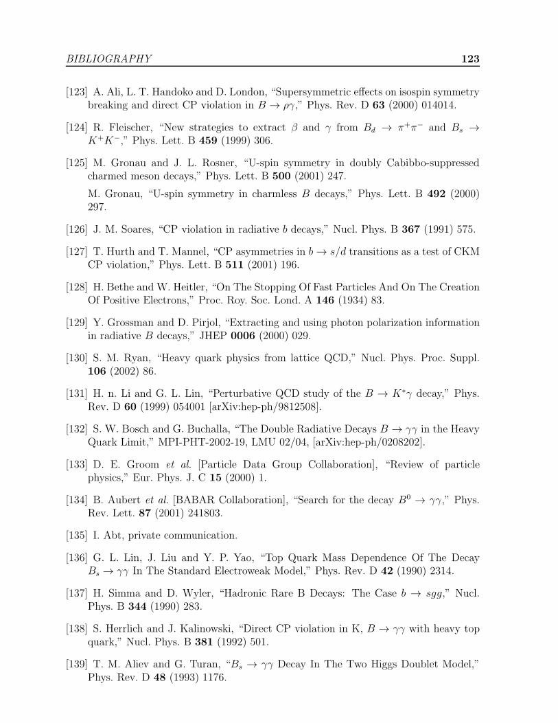
BIBLIOGRAPHY 123
[123] A. Ali, L. T. Handoko and D. London, “Supersymmetric effects on isospin symmetrybreaking and direct CP violation in B → ργ,” Phys. Rev. D 63 (2000) 014014.
[124] R. Fleischer, “New strategies to extract β and γ from Bd → π+π− and Bs →K+K−,” Phys. Lett. B 459 (1999) 306.
[125] M. Gronau and J. L. Rosner, “U-spin symmetry in doubly Cabibbo-suppressedcharmed meson decays,” Phys. Lett. B 500 (2001) 247.
M. Gronau, “U-spin symmetry in charmless B decays,” Phys. Lett. B 492 (2000)297.
[126] J. M. Soares, “CP violation in radiative b decays,” Nucl. Phys. B 367 (1991) 575.
[127] T. Hurth and T. Mannel, “CP asymmetries in b→ s/d transitions as a test of CKMCP violation,” Phys. Lett. B 511 (2001) 196.
[128] H. Bethe and W. Heitler, “On The Stopping Of Fast Particles And On The CreationOf Positive Electrons,” Proc. Roy. Soc. Lond. A 146 (1934) 83.
[129] Y. Grossman and D. Pirjol, “Extracting and using photon polarization informationin radiative B decays,” JHEP 0006 (2000) 029.
[130] S. M. Ryan, “Heavy quark physics from lattice QCD,” Nucl. Phys. Proc. Suppl.106 (2002) 86.
[131] H. n. Li and G. L. Lin, “Perturbative QCD study of the B → K∗γ decay,” Phys.Rev. D 60 (1999) 054001 [arXiv:hep-ph/9812508].
[132] S. W. Bosch and G. Buchalla, “The Double Radiative Decays B → γγ in the HeavyQuark Limit,” MPI-PHT-2002-19, LMU 02/04, [arXiv:hep-ph/0208202].
[133] D. E. Groom et al. [Particle Data Group Collaboration], “Review of particlephysics,” Eur. Phys. J. C 15 (2000) 1.
[134] B. Aubert et al. [BABAR Collaboration], “Search for the decay B0 → γγ,” Phys.Rev. Lett. 87 (2001) 241803.
[135] I. Abt, private communication.
[136] G. L. Lin, J. Liu and Y. P. Yao, “Top Quark Mass Dependence Of The DecayBs → γγ In The Standard Electroweak Model,” Phys. Rev. D 42 (1990) 2314.
[137] H. Simma and D. Wyler, “Hadronic Rare B Decays: The Case b → sgg,” Nucl.Phys. B 344 (1990) 283.
[138] S. Herrlich and J. Kalinowski, “Direct CP violation in K, B → γγ with heavy topquark,” Nucl. Phys. B 381 (1992) 501.
[139] T. M. Aliev and G. Turan, “Bs → γγ Decay In The Two Higgs Doublet Model,”Phys. Rev. D 48 (1993) 1176.
124 BIBLIOGRAPHY
[140] G. G. Devidze, G. R. Dzhibuti and A. G. Liparteliani, “On The Double RadiativeDecays Of The Bs Meson And µ Atom: Bs → γγ, µ+e− → γγ,” Nucl. Phys. B 468(1996) 241.
[141] G. Hiller and E. O. Iltan, “Leading logarithmic QCD corrections to the Bs → γγdecay rate including long-distance effects through Bs → Φγ → γγ,” Phys. Lett. B409 (1997) 425;
[142] G. Hiller and E. O. Iltan, “Estimate of the long-distance contribution through b→sψ to the Bs → γγ decay rate,” Mod. Phys. Lett. A 12 (1997) 2837.
[143] L. Reina, G. Ricciardi and A. Soni, “QCD corrections to b → sγγ induced decays:B → Xsγγ and Bs → γγ,” Phys. Rev. D 56 (1997) 5805.
[144] C. V. Chang, G. Lin and Y. Yao, “QCD corrections to b → sγγ and exclusiveBs → γγ decay,” Phys. Lett. B 415 (1997) 395.
[145] J. Cao, Z. Xiao and G. Lu, “The B → Xsγγ decay in the standard model and thegeneral two-Higgs-doublet model,” Phys. Rev. D 64 (2001) 014012.
[146] J. O. Eeg, K. Kumericki and I. Picek, “The double radiative annihilation of theheavy-light fermion bound states,” arXiv:hep-ph/0203055.
[147] G. P. Korchemsky, D. Pirjol and T. M. Yan, “Radiative leptonic decays of B mesonsin QCD,” Phys. Rev. D 61 (2000) 114510.
[148] M. Bander, D. Silverman and A. Soni, “CP Noninvariance In The Decays Of HeavyCharged Quark Systems,” Phys. Rev. Lett. 43 (1979) 242.
[149] D. Choudhury and J. R. Ellis, “Estimates of long-distance contributions to theBs → γγ decay,” Phys. Lett. B 433 (1998) 102.
[150] W. Liu, B. Zhang and H. Zheng, “On the long distance contribution to the Bs → γγdecay in the effective Lagrangian approach,” Phys. Lett. B 461 (1999) 295.
[151] S. Fajfer, P. Singer and J. Zupan, “The rare decay D0 → γγ,” Phys. Rev. D 64(2001) 074008.
[152] G. Burdman, E. Golowich, J. Hewett and S. Pakvasa, “Rare charm decays in thestandard model and beyond,” arXiv:hep-ph/0112235.
[153] M. Neubert, “Heavy quark symmetry,” Phys. Rept. 245 (1994) 259 and referencestherein.
[154] C. Greub, T. Hurth, M. Misiak and D. Wyler, “The c→ uγ Contribution to WeakRadiative Charm Decay,” Phys. Lett. B 382 (1996) 415.
[155] M. Acciarri et al. [L3 Collaboration], “Search for the decays B(d)0→ gamma gammaand B(s)0 → gamma gamma,” Phys. Lett. B 363 (1995) 137.
[156] “Physics at a 10**36 asymmetric B factory,” SLAC-PUB-8970.

BIBLIOGRAPHY 125
[157] T. Altomari, “Contribution Of Exclusive Decays B → K∗∗(I)γ To B → sγ,” Phys.Rev. D 37 (1988) 677.
A. Ali, T. Ohl and T. Mannel, “Radiative rare B decays into higher K resonances,”Phys. Lett. B 298 (1993) 195 [arXiv:hep-ph/9208207].
S. Veseli and M. G. Olsson, “Radiative rare B decays revisited,” Phys. Lett. B 367(1996) 309 [arXiv:hep-ph/9508255].
D. Ebert, R. N. Faustov, V. O. Galkin and H. Toki, “Rare radiative B decays toorbitally excited K mesons,” Phys. Rev. D 64 (2001) 054001.
A. S. Safir, “The radiative rare decays B → K∗∗γ in the light-cone QCD sum ruleapproach,” Eur. Phys. J. directC 15 (2001) 1.
[158] K. Abe et al. [Belle Collaboration], “Observation of radiative B meson decays intohigher kaonic resonances,” arXiv:hep-ex/0107065.
[159] citation found in: C. Quigg, “Visions: The coming revolutions in particle physics,”arXiv:hep-ph/0204075.
[160] A. J. Buras, M. Misiak, M. Munz and S. Pokorski, “Theoretical uncertainties andphenomenological aspects of B → Xsγ decay,” Nucl. Phys. B 424 (1994) 374.

126 BIBLIOGRAPHY
Acknowledgements
I want to thank everybody who helped this thesis coming into being.
In the first place I thank Gerhard Buchalla for his exclusive support. He suggested andvery pedagogically introduced me to the subject of this work. At any time he was readyto discuss my questions and ideas. I could learn a lot from him. I also want to thankhim for the assistance in arranging my stay at the CERN Theory Division where ourcollaboration started.
I thank Andrzej Buras for supervising my thesis. I highly value his fatherly advice and thediscussions with him. With all my ventures I always could rely on his quick and favourablesupport. I am grateful to Gerhard and Andrzej also for proofreading the manuscript.
I very much appreciate the kind hospitality of the CERN Theory Division during the tenmonths I stayed there and the visits afterwards. To all friends and colleagues at CERNand the Max-Planck-Institut fur Physik I am grateful for stimulating discussions andcreating a very pleasant social environment. In particular the lunch time conversationswith Edda, Emmanuel, both Haralds, Johannes, Karsten, Martin, the two Peters, Roman,Werner, and the rest of the “Austrian gang” at CERN and Amol, Andre, Ariel, Bjorn,Dima, Gennaro, Georg, Mathias, Michael, Pavel, Pushan, Ralf, Ricard, Robert, Sergio,and Thomas at the MPI will stick lively in my mind. Thanks to the members of AndrzejBuras’s chair and here especially my co-postgraduates Martin, Sebastian, and Uli for theconvivial receptions in Garching and helpful discussions.
A great thankyou to my parents and my whole family for all their unconditional supportof any kind, the interest in my work, and for keeping me grounded. Last, but definitelynot least, it is a great pleasure to express my warmest thanks to Caroline.
I gratefully acknowledge financial support of the Max-Planck-Gesellschaft and the Stu-dienstiftung des deutschen Volkes during my time in Munich and Geneva, respectively.