Exchange Rates, Local Currency Pricing andInternational Tax Policies

Sihao Chen∗

HKUSTMichael B. Devereux

UBCKang ShiCUHK

Juanyi XuHKUST

June 19, 2019

Abstract

Empirical evidence suggests that for many countries, retail prices of tradedgoods are sticky in national currencies. Movements in exchange rates thencause deviations from the law of one price, and exchange rate misalignment,which cannot be corrected by monetary policy alone. This paper shows thata state contingent international tax policy can be combined with monetarypolicy to eliminate exchange rate misalignment and sustain a fully efficientwelfare outcome. But this monetary-fiscal mix cannot be decentralized withnon-cooperative determination of monetary and fiscal policy. Non-cooperativeuse of taxes and subsidies introduces strategic spillovers which opens up a fun-damental conflict between the goals of output gap and inflation stabilizationand those of terms of trade manipulation in an open economy. The implemen-tation of an efficient monetary-fiscal mix requires effective cooperation in fiscalpolicy, while leaving monetary policy to be determined non-cooperatively. Inaddition, while an efficient outcome requires state contingent taxes and sub-sidies to eliminate exchange rate misalignment, it is still necessary to haveflexible exchange rates and independent monetary policy.

JEL classification: F3, F4

Keywords: local currency pricing, international tax, exchange rate; policy coordi-

nation;

∗Chen: Department of Economics, Hong Kong University of Science and Technology, Email:housechen90@gmail.com; Devereux: Vancouver School of Economics, University of BritishColumbia, Email: Michael.Devereux@ubc.ca; Shi: Department of Economics, The Chinese Uni-versity of Hong Kong, Email: kangshi@cuhk.edu.hk; Xu: Department of Economics, Hong KongUniversity of Science and Technology, Email: jennyxu@ust.hk. Devereux acknowledges financialsupport from the Social Sciences and Research Council of Canada. Xu would like to thank theHong Kong Research Grants Council (GRF No. 644810) for financial support.

1 Introduction

This paper is a theoretical exploration of the optimal combination of monetary and

fiscal policy in a global economy with sticky prices, local currency pricing, and

exchange rate misalignment. In this environment, monetary policy alone cannot

achieve a fully efficient allocation. A combination of monetary and fiscal policy

might do better. But in a world of independent policy-makers, the introduction of

additional fiscal tools into the policy process can generate new strategic inefficiencies.

The benefit of flexible exchange rates represents a central pillar of open econ-

omy macroeconomics. Famously, Friedman (1953) argued for the ease of adjusting

relative prices with nominal exchange rates as opposed to nominal prices in an

environment of sticky prices. The extension of the Friedman case for flexible ex-

changes rate is that it allows for national monetary independence. With flexible

exchange rates, individual countries can follow independent, or ‘self-oriented’ mon-

etary policies (using the language of Obstfeld and Rogoff, 2002), without requiring

international policy coordination.

The more recent New Keynesian open economy literature has articulated Fried-

man’s insights in fully specified welfare-based DSGE models. In particular Clar-

ida, Gali and Gertler (2002) and Obstfeld and Rogoff (2002) show that an optimal

monetary policy requires flexible exchange rates, and in certain environments, self-

oriented monetary policy-making can achieve a global optimum, without the need

for (or any benefit from) international policy coordination.1 Both these papers

however follow the traditional assumption about traded goods pricing, notably that

prices are set in producer’s currency (PCP).

Recent contributions have qualified these arguments, based on the evidence that

nominal exchange rate adjustment may fail to achieve efficient relative price adjust-

ment. For instance, when traded goods prices are set in the currency of the buyer

1Many other papers have analyzed non-cooperative monetary policy in open economies. See

for instance Corsetti and Pesenti, 2001, and Corsetti, Dedola and Leduc, 2010. We discuss the

literature more fully below.

1

(local currency pricing, or LCP), movements in nominal exchange rates will gener-

ate deviations from the law of one price across countries. In this case, independent

monetary policy and flexible exchange rates cannot fully undo the inefficiencies gen-

erated by nominal price stickiness. Engel (2011) constructs a New Keynesian open

economy model with LCP, and shows that optimal monetary policy faces a trade-off

between the output gap, inflation control, and exchange rate ‘misalignment’ due to

deviations from the law of one price. Then even cooperative monetary policy-making

cannot achieve a full global optimum.

Fujiwara and Wang (2017) extend Engel’s model to the case of non-cooperative

policy making. They identify a new set of strategic inefficiencies associated with

non-cooperative policy-making in an environment of LCP, and show that in general

there are positive gains to policy-coordination under LCP, even in the case where

no such gains would exist with PCP.

A separate and more recent literature has widened the debate on the limits to

monetary policy by exploring the possibility of using targeted fiscal instruments to

achieve effective relative price adjustment even when nominal prices cannot move.

One strand of this literature is motivated by the constraints of a single currency

area, where by definition nominal exchange rates cannot respond to country specific

shocks. For instance, Fahri, Gopinath and Itskhoki (2013) show that a set of taxes

and subsidies can replicate an exchange rate devaluation under a fixed exchange

rate regime. Other papers are motivated by the limits to monetary policy imposed

by the zero lower bound (see for instance, Correa, Fahri, Nicolini, and Teles 2013).

But local currency pricing also imposes limits on the ability of monetary policy to

achieve fully efficient outcomes. Somewhat less attention has been paid to this case.2

2A notable exception is Adao Correa and Teles 2009, who derive a set of tax policies that can

achieve an efficient global outcome independent of the type of nominal price stickiness. The key

difference between their paper and ours, aside from using different instruments and a different

assumption about financial markets (see below) is that we look at the implementability of these

policies in a non-cooperative setting. We discuss their paper in more detail below.

2

Can these constraints be undone by targeted sets of taxes and subsidies?

This paper first outlines a set of import taxes and export subsidies that can

eliminate the distortions imposed by deviations from the law of one price. Do these

fiscal instruments then restore the efficacy of monetary policy and the benefits of

flexible exchange rates, or alternatively, would they eliminate the need for exchange

rate adjustment at all?

But the main question we address is whether the use of fiscal instruments re-

stores the case for self-oriented policymaking (monetary independence). As noted

above, Fujiwara and Wang (2017) show that there are losses from non-cooperative

policy making under LCP. If policy makers have access to taxes and subsidies that

can eliminate deviations from the law of one price (or exchange rate misalignment),

does this imply that independent non-cooperative policy making can sustain full ef-

ficiency? Alternatively, one might conjecture that the addition of independent fiscal

policy instruments into policy-making introduces a new set of strategic inefficiencies

in independent policymaking.

We construct a two country open economy model under LCP along the lines of

Engel (2011) and Fujiwara and Wang (2017). Each country is subject to random

shocks to labour productivity. Generically, this environment is characterized by

exchange rate misalignment, causing welfare losses due to deviations from the law

of one price. We then identify a set of taxes and subsidies that can eliminate

inefficiencies coming from these deviations from the law of one price. In particular,

in response to a home country (positive) productivity shock, an optimal policy

entails a positive home country tax on imports and a foreign country subsidy to

exports, combined with the opposite response of the foreign import tax and the home

export subsidy. This set of tax-subsidy responses can perfectly replicate the relative

price movement that would take place under PCP, eliminating deviations from the

law of one price. Intuitively, this tax-subsidy combination will lead consumers and

producers to tilt their behaviour as if all prices were set in producer’s currency and

there existed full exchange rate pass-through in traded goods prices. The import

3

tax is set so that, given prices set by producers, consumers face the same price for

a good across countries, while the export subsidy is set so that producer’s price

setting is not distorted by the import tax itself.

An interesting feature of this optimal policy mix is that it does not obviate the

need for exchange rate adjustment. Conditional on the optimal taxes and subsidies,

an optimal monetary rule requires that the exchange rate adjusts to productivity

shocks exactly as would occur under PCP. Thus, the use of optimal taxes and

subsides restores Friedman’s ‘case for flexible exchange rates’.

But the key question is whether this efficient policy mix is consistent with non-

cooperative policy-making? In the absence of coordination, both taxes, subsidies,

and monetary policy have to be chosen by individual authorities. Here, our results

are quite striking. We show the choice of import taxes and export subsidies opens

up a new strategic channel in non-cooperative policy making associated with terms

of trade manipulation. Acting independently, each policymaker attempts to bias

the tax-subsidy instruments so as to raise its expected terms of trade. We show

that when the tax-subsidy choice is unrestricted, there is no equilibrium to the

non-cooperative game consistent with finite inflation rates and output gaps.3

We address this dilemma in two ways. First, we show that if we impose a partic-

ular restriction on the set of import taxes and export subsidies, then the equilibrium

of the non-cooperative game will coincide with the cooperative equilibrium, and will

attain the flexible price equilibrium. In particular this condition requires that the

home import tax be restricted to equal the foreign export subsidy.

But this restriction may seem somewhat arbitrary, and it is unclear how it would

be imposed in a non-cooperative equilibrium. To resolve this, we conclude that an

3We note that the channel of terms of trade manipulation in optimal monetary policy has been

explored extensively in the New Keynesian literature. See for instance Corsetti and Pesenti, 2001,

and Clarida Gali and Gertler 2002 for early discussion. But our results are quite different from

the conventional analysis. We show that this strategic inefficiency is generated solely by the use

of state varying fiscal instruments in monetary policy. Without the use of fiscal instruments, the

equilibrium under non-cooperative monetary policy is well defined, as in Fujiwara and Wang 2017.

4

efficient monetary-fiscal mix will require fiscal policy coordination. We define a

new game in which taxes and subsidies are chosen by a cooperative fiscal authority

maximizing world welfare, while monetary policy is determined independently by

each monetary authority. We show that the equilibrium of this game will be the

same as the cooperative equilibrium in which both fiscal and monetary policy are

chosen by a single benevolent authority.

The implication of these results is then clear - an optimally chosen set of fiscal

responses can eliminate the restrictions on monetary policy implied by LCP, and

restore the benefits of flexible exchange rates. But in order for this to be consistent

with independent ‘self-reliance’ in monetary policy, it is necessary to have effective

coordination in fiscal policy. Alternatively, the message could be interpreted as

saying that absent fiscal coordination, or effective restrictions on fiscal responses,

the use of taxes and subsidies to correct deviations from the law of one price and

support independent policy-making cannot be successful.

An interesting feature of our results is that the use of optimal tax-subsidies

changes the nature of optimal monetary policy under LCP. Engel (2011) shows that

with LCP, the monetary authority should target consumer price inflation instead of

producer-price inflation, as this sustains more efficient risk-sharing, even when LCP

prevents a fully efficient allocation. We show that, so long as fiscal instruments are

set optimally so as to achieve efficient risk sharing and eliminating deviations from

the law of one price, the monetary authority should once again target producer price

inflation rather than CPI inflation, even in the presence of LCP.

The tax-subsidy mix that we highlight is not the only set of fiscal instruments

that can achieve an efficient global outcome. In a later section of the paper, in-

spired by the paper of Adao et al. (2009), we show that an alternative set of tax

instruments, namely goods-specific consumption taxes and a tax on labor income,

can be used to sustain an efficient global allocation, eliminating deviations from the

law of one price and at the same time achieving efficient risk-sharing.4 But again,

4One important difference is that this set of policy tools requires a fixed nominal exchange rate,

5

we find that this allocation cannot be sustained by non-cooperative policy-making,

for identical reasons as in our main model.

A final section of the paper presents a quantitative analysis of welfare gains. The

welfare gains from correcting currency misalignments under a cooperative monetary

policy are very small. But the welfare gains from an optimal monetary fiscal-mix,

compared to a non-cooperative monetary policy equilibrium under LCP, while still

small in absolute terms, are substantially larger.5

This paper is organized as follows. Section 2 discusses the related literature. Sec-

tion 3 presents the benchmark dynamic model with staggered price setting under

LCP, and establishes that a combination of import tariffs (or equivalently, consump-

tion taxes on foreign goods) and a monetary policy that stabilizes producer prices

can sustain a fully efficient outcome. Section 4 take a special case of the model in

which all results can be derived analytically. Using this special case, we show that

the set of optimal import taxes and export subsidies which sustain full efficiency can-

not be achieved in a non-cooperative equilibrium. There are no finite tax-subsidy

combinations that solve the non-cooperative game. Section 5 derives the results in

the general dynamic model using second order approximations to country welfare

functions. Then the main results on cooperative and non-cooperative policy-making

in the dynamic model are derived. Section 6 discusses the results under an alterna-

tive set of taxes. Section 7 provides some welfare results. Finally section 8 presents

some conclusions.

2 Related Literature

Our paper is related to the literature on optimal fiscal policy in open economies.

Gali and Monacelli (2008) study how the government chooses the optimal level of

as explained in section (6)5This is in accord with the results of Fujiwara and Wang (2017), who quantify the welfare gains

from monetary policy cooperation under LCP.

6

public consumption in a monetary union with lump-sum taxes. They find that the

choice of fiscal policy raises union welfare. Hevia and Nicolini (2013) consider a

small open economy with flexible exchange rates and state-contingent assets. They

find that flexible price equilibrium is implementable, but exchange rates must move

across states. Benigno and Paoli (2010) also analyze optimal fiscal policy and in

small open economy, but in their set-up, the optimal flexible price allocation cannot

be achieved.

Our paper is complementary to Adao, Correia, and Teles (2009). They show

that in an environment with nominal rigidities, whatever is the type of price set-

ting (PCP or LCP), the exchange rate regime, whether flexible or fixed exchange

rates, is irrelevant once fiscal policy instruments (both taxes on labor income and

consumption of home and foreign goods) are taken into account. Hence fiscal policy

instruments can replicate the flexible price equilibrium even under LCP. They derive

these results using a Ramsey approach, which requires a benevolent social planner

who can use the available policy instruments to replicate the flexible price allocation.

This approach abstracts from the question of how to implement the optimal fiscal

policy in a non-cooperative setting, which is the main focus of our paper. We show

that in an environment where monetary policy is chosen by individual countries we

can achieve a fully efficient flexible price equilibrium, so long as taxes and subsidies

are chosen cooperatively.

Another important difference between our paper and theirs is related to the

role of exchange rate flexibility. They find that the flexible price allocation can be

achieved by fiscal and monetary policies that induce stable producer prices and with-

out relying on exchange rate movements. In fact the exchange rate regime becomes

irrelevant. But in our benchmark model, it is critical to allow for flexible exchange

rates, in order to achieve complete risk sharing. The optimal response of import

taxes in each country ensures that relative prices facing households respond in the

right way to productivity shocks. For instance, after a home country productivity

shock the home import tax should rise, while the foreign import tax should fall.

7

But on their own, this would imply an appreciation of the home real exchange rate.

To counter this, monetary policy must facilitate a nominal depreciation in order

to ensure efficient risk-sharing. Hence, the tax policies identified in our paper not

only replicate the real variables under a flexible price allocation, but also replicate

the efficient risk-sharing response of the exchange rate fluctuations under flexible

prices.6

Our paper also belongs to a small but fast growing literature that emphasizes

the role of fiscal policy in replacing monetary policy or exchange rate policy as a

macro stabilization tool. Schmitt-Grohe and Uribe (2011) show that, when there

are downward wage rigidity and inelastic labor supply, a payroll subsidy alone can

replicate the effect of nominal exchange rate devaluation. Farhi, Gopinath and It-

skhoki (2013) show that, when the exchange rate cannot be devalued, a small set

of conventional fiscal instruments can robustly replicate the real allocation attained

under a nominal exchange rate devaluation in a dynamic New Keynesian open econ-

omy environment. In both these papers, the assumption is that nominal exchange

rate is fixed, perhaps due to membership of a single currency area. In contrast,

the exchange rate regime is flexible in our model, but exchange rate changes are

inefficient due to LCP.

As mentioned in the introduction, the addition of fiscal instruments to substitute

or complement monetary policy may also introduce strategic spillover channels when

we extend the analysis to study non-cooperative policy-making. A key result of our

6Adao, Correia, and Teles 2009 also differ from us in the nature of financial markets. They

allow for two state-contingent domestic bonds, but in their model there are no state-contingent

international bonds. So there is not risk-sharing across countries in their baseline model. When

state-contingent bonds can be traded across countries, they show that an extra fiscal instrument,

a state-contingent government bond, is needed to produce the irrelevance result. Our framework

by contrast is based on the assumption of complete markets for cross-country risk-sharing. Section

6 below allows for a labor income tax and consumption tax in our model, and shows that while

a cooperative equilibrium can sustain full efficiency, albeit with a fixed exchange rate, the non-

cooperative game has the same features as in our benchmark model.

8

paper is that absent some additional constraints on the design of corrective taxes or

subsidies, in an environment where policy-makers act independently, these strategic

inefficiencies may render fiscal policy ineffective in correcting macro inefficiencies.

Finally, topic wise, this paper is also closely related to the literature on optimal

monetary policy in open economy under LCP. This question is treated in Devereux

and Engel (2003). As discussed above, Engel (2011) shows that even with policy co-

ordination, optimal monetary policy cannot replicate the flexible price equilibrium,

due to the currency misalignment induced by LCP. Fujiwara and Wang (2017) focus

on a non-cooperative game under LCP in a two-country dynamic general equilibrium

model. They find that in this case, policy makers face extra trade-offs regarding

stabilizing real marginal cost induced by the deviations from law of one price. Both

papers therefore emphasize the importance of currency misalignment in the optimal

monetary policy. Our paper identifies the a monetary-fiscal mix that can correct

this misalignment, but also the restrictions on independent policy-making required

to implement such a policy. The main difference between our paper and Engel

(2011) or Fujiwara and Wang (2017) is that we introduce two fiscal instruments so

as to eliminate the distortions caused by LCP, an import tax on imported goods

and an export subsidy on export goods.

3 Model

We first set out the baseline model, and show the general result that an optimal

monetary policy combined with a tax-subsidy scheme can support the fully efficient

flexible price equilibrium. The model is similar to Engel (2011) and Fujiwara and

Wang (2017), who make special functional form assumptions. We follow these as-

sumptions since they will be used to derive the results in the dynamic game using

approximated welfare functions in subsequent sections. But the main results of this

section hold in a much more general model, which we show in Technical Appendix

Section (2).

9

There are two countries of equal size, denoted Home and Foreign, each popu-

lated with a continuum of households with population size normalized to unity. In

each country, households consume both home and foreign goods with a symmetric

home bias. They supply labor to firms in a competitive labor market. Firms are

monopolistically competitive and produce differentiated goods. They set prices, in

local currency, in a staggered manner, as in Calvo (1983). The government levies a

lump-sum tax on households and subsidizes firms to eliminate steady-state distor-

tions from monopolistic pricing. As in most of the existing literature we assume a

complete financial market.

3.1 Household

The representative home household is assumed to maximize lifetime utility, defined

as,

U = E∞t=0βt(C1−ρt

1− ρ− ηLt + χ log(

Mt

Pt)) (3.1)

Consumption Ct is a Cobb-Douglas aggregation of home goods and foreign

goods. Ct = Cv2htC

1− v2

ft , where v ≥ 1 denotes the degree of home bias in consump-

tion. Both home and foreign goods consumption is differentiated into a measure

1 of varieties with a constant elasticity of substitution among varieties equal to

λ. The consumption-based price index is Pt = Θ−1Pv2hh,t((1 + tc,t)Pfh,t)

1− v2 , where

Θ = (v2)v2 (1− v

2)1−

v2 . Phht and Pfht represent the (home currency) price set by home

and foreign firms, respectively, for sale in the home market. tc,t is a state-contingent

import tax imposed on foreign goods. It is standard in the literature to derive the

equilibrium as χ −→ 0, and hence ignore the role of money in welfare.

The demand for home and foreign goods is Ch,t=v2PtCtPhht

and Cf,t=(1−v2) PtCtPfh,t(1+tc,t)

.

The budget constraint under complete markets is given by

PtCt+Bht+1+∑

ζt+1∈Zt+1

B(ζt+1|ζt)D(ζt+1) = WtLt+Rt−1Bh,t+Πt+Tt+D(ζt), (3.2)

10

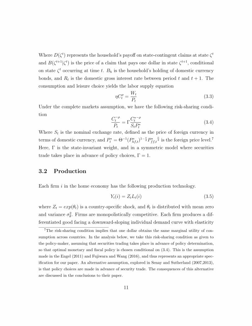
Where D(ζt) represents the household’s payoff on state-contingent claims at state ζt

and B(ζt+1|ζt) is the price of a claim that pays one dollar in state ζt+1, conditional

on state ζt occurring at time t. Bh is the household’s holding of domestic currency

bonds, and Rt is the domestic gross interest rate between period t and t + 1. The

consumption and leisure choice yields the labor supply equation

ηCρt =

Wt

Pt(3.3)

Under the complete markets assumption, we have the following risk-sharing condi-

tionC−ρtPt

= ΓC∗t−ρ

StP ∗t(3.4)

Where St is the nominal exchange rate, defined as the price of foreign currency in

terms of domestic currency, and P ∗t = Θ−1(P ∗hf,t)1− v

2P ∗ff,tv2 is the foreign price level.7

Here, Γ is the state-invariant weight, and in a symmetric model where securities

trade takes place in advance of policy choices, Γ = 1.

3.2 Production

Each firm i in the home economy has the following production technology.

Yt(i) = ZtLt(i) (3.5)

where Zt = exp(θt) is a country-specific shock, and θt is distributed with mean zero

and variance σ2θ . Firms are monopolistically competitive. Each firm produces a dif-

ferentiated good facing a downward-sloping individual demand curve with elasticity

7The risk-sharing condition implies that one dollar obtains the same marginal utility of con-

sumption across countries. In the analysis below, we take this risk-sharing condition as given to

the policy-maker, assuming that securities trading takes place in advance of policy determination,

so that optimal monetary and fiscal policy is chosen conditional on (3.4). This is the assumption

made in the Engel (2011) and Fujiwara and Wang (2016), and thus represents an appropriate spec-

ification for our paper. An alternative assumption, explored in Senay and Sutherland (2007,2013),

is that policy choices are made in advance of security trade. The consequences of this alternative

are discussed in the conclusions to their paper.

11

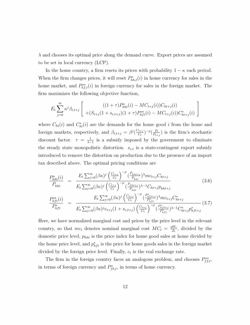
λ and chooses its optimal price along the demand curve. Export prices are assumed

to be set in local currency (LCP).

In the home country, a firm resets its prices with probability 1− κ each period.

When the firm changes prices, it will reset P ohh,t(i) in home currency for sales in the

home market, and P o∗hf,t(i) in foreign currency for sales in the foreign market. The

firm maximizes the following objective function,

Et

∞∑j=0

κjβt,t+j

[((1 + τ)P o

hht(i)−MCt+j(i))Cht+j(i)

+(St+j(1 + se,t+j)(1 + τ)P o∗hft(i)−MCt+j(i))C

∗ht+j(i)

]

where Cht(i) and C∗ht(i) are the demands for the home good i from the home and

foreign markets, respectively, and βt,t+j = βj(Ct+jCt

)−ρ( PtPt+j

) is the firm’s stochastic

discount factor. τ = 1λ−1 is a subsidy imposed by the government to eliminate

the steady state monopolistic distortion. se,t is a state-contingent export subsidy

introduced to remove the distortion on production due to the presence of an import

tax described above. The optimal pricing conditions are

P ohht(i)

Phht=

Et∑∞

j=0(βκ)j(Ct+jCt

)−ρ(Phht+jPhht

)λmct+jCht+j

Et∑∞

j=0(βκ)j(Ct+jCt

)−ρ(Phht+jPhht

)λ−1Cht+jphht+j

(3.6)

P o∗hft(i)

P ∗hft=

Et∑∞

j=0(βκ)j(Ct+jCt

)−ρ(P ∗hft+j

P ∗hft

)λmct+jC∗ht+j

Et∑∞

j=0(βκ)jet+j(1 + se,t+j)(Ct+jCt

)−ρ(P ∗hft+j

P ∗hft

)λ−1C∗ht+jp∗hft+j

(3.7)

Here, we have normalized marginal cost and prices by the price level in the relevant

country, so that mct denotes nominal marginal cost MCt = ηWt

Zt, divided by the

domestic price level, phht is the price index for home good sales at home divided by

the home price level, and p∗hft is the price for home goods sales in the foreign market

divided by the foreign price level. Finally, et is the real exchange rate.

The firm in the foreign country faces an analogous problem, and chooses P ∗off,t,

in terms of foreign currency and P ofh,t, in terms of home currency.

12

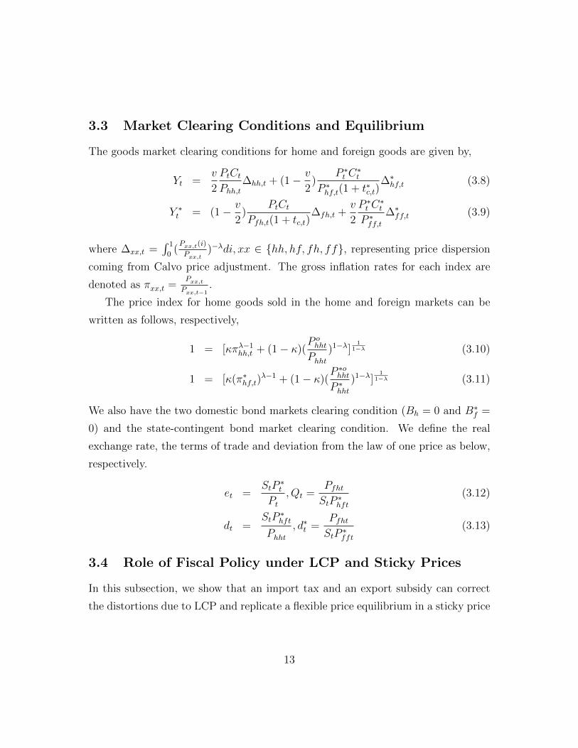
3.3 Market Clearing Conditions and Equilibrium

The goods market clearing conditions for home and foreign goods are given by,

Yt =v

2

PtCtPhh,t

∆hh,t + (1− v

2)

P ∗t C∗t

P ∗hf,t(1 + t∗c,t)∆∗hf,t (3.8)

Y ∗t = (1− v

2)

PtCtPfh,t(1 + tc,t)

∆fh,t +v

2

P ∗t C∗t

P ∗ff,t∆∗ff,t (3.9)

where ∆xx,t =∫ 1

0(Pxx,t(i)

Pxx,t)−λdi, xx ∈ {hh, hf, fh, ff}, representing price dispersion

coming from Calvo price adjustment. The gross inflation rates for each index are

denoted as πxx,t =Pxx,tPxx,t−1

.

The price index for home goods sold in the home and foreign markets can be

written as follows, respectively,

1 = [κπλ−1hh,t + (1− κ)(P ohht

Phht)1−λ]

11−λ (3.10)

1 = [κ(π∗hf,t)λ−1 + (1− κ)(

P ∗ohhtP ∗hht

)1−λ]1

1−λ (3.11)

We also have the two domestic bond markets clearing condition (Bh = 0 and B∗f =

0) and the state-contingent bond market clearing condition. We define the real

exchange rate, the terms of trade and deviation from the law of one price as below,

respectively.

et =StP

∗t

Pt, Qt =

PfhtStP ∗hft

(3.12)

dt =StP

∗hft

Phht, d∗t =

PfhtStP ∗fft

(3.13)

3.4 Role of Fiscal Policy under LCP and Sticky Prices

In this subsection, we show that an import tax and an export subsidy can correct

the distortions due to LCP and replicate a flexible price equilibrium in a sticky price

13

model.8 We first describe the efficient allocation and then highlight the role that

fiscal instruments play in eliminating the distortions due to LCP.

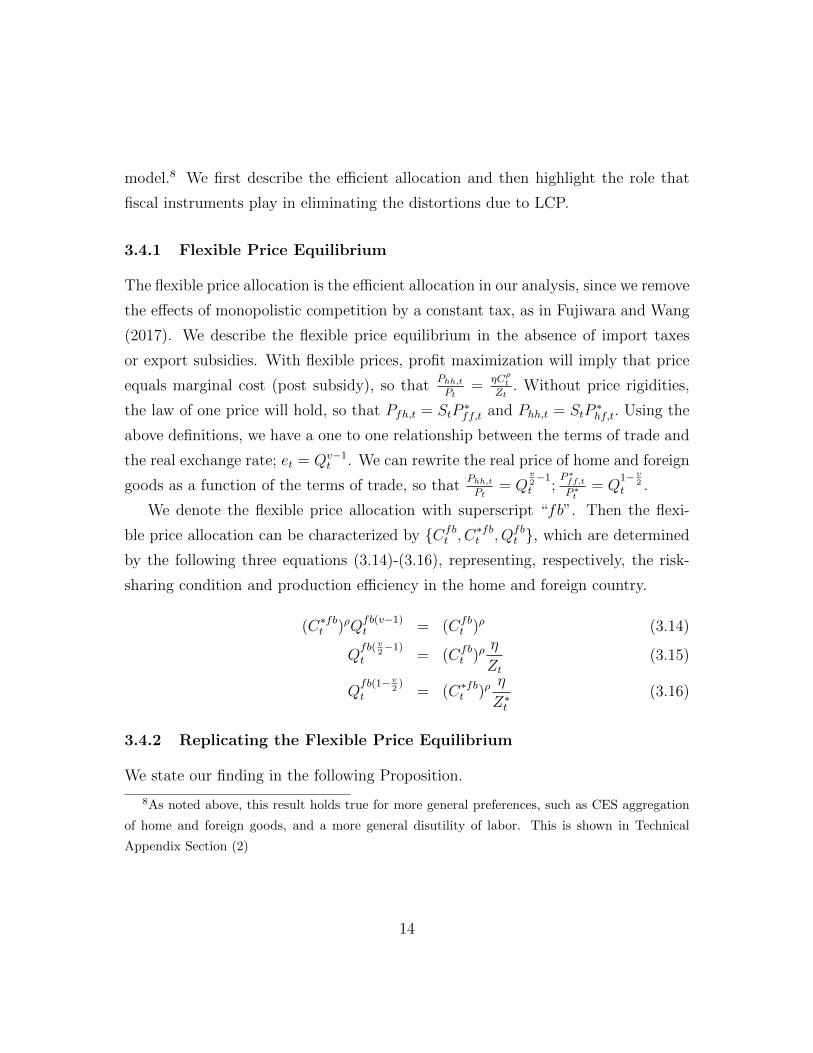
3.4.1 Flexible Price Equilibrium

The flexible price allocation is the efficient allocation in our analysis, since we remove

the effects of monopolistic competition by a constant tax, as in Fujiwara and Wang

(2017). We describe the flexible price equilibrium in the absence of import taxes

or export subsidies. With flexible prices, profit maximization will imply that price

equals marginal cost (post subsidy), so thatPhh,tPt

=ηCρtZt. Without price rigidities,

the law of one price will hold, so that Pfh,t = StP∗ff,t and Phh,t = StP

∗hf,t. Using the

above definitions, we have a one to one relationship between the terms of trade and

the real exchange rate; et = Qv−1t . We can rewrite the real price of home and foreign

goods as a function of the terms of trade, so thatPhh,tPt

= Qv2−1

t ;P ∗ff,t

P ∗t

= Q1− v

2t .

We denote the flexible price allocation with superscript “fb”. Then the flexi-

ble price allocation can be characterized by {Cfbt , C

∗fbt , Qfb

t }, which are determined

by the following three equations (3.14)-(3.16), representing, respectively, the risk-

sharing condition and production efficiency in the home and foreign country.

(C∗fbt )ρQfb(v−1)t = (Cfb

t )ρ (3.14)

Qfb( v

2−1)

t = (Cfbt )ρ

η

Zt(3.15)

Qfb(1− v

2)

t = (C∗fbt )ρη

Z∗t(3.16)

3.4.2 Replicating the Flexible Price Equilibrium

We state our finding in the following Proposition.

8As noted above, this result holds true for more general preferences, such as CES aggregation

of home and foreign goods, and a more general disutility of labor. This is shown in Technical

Appendix Section (2)

14

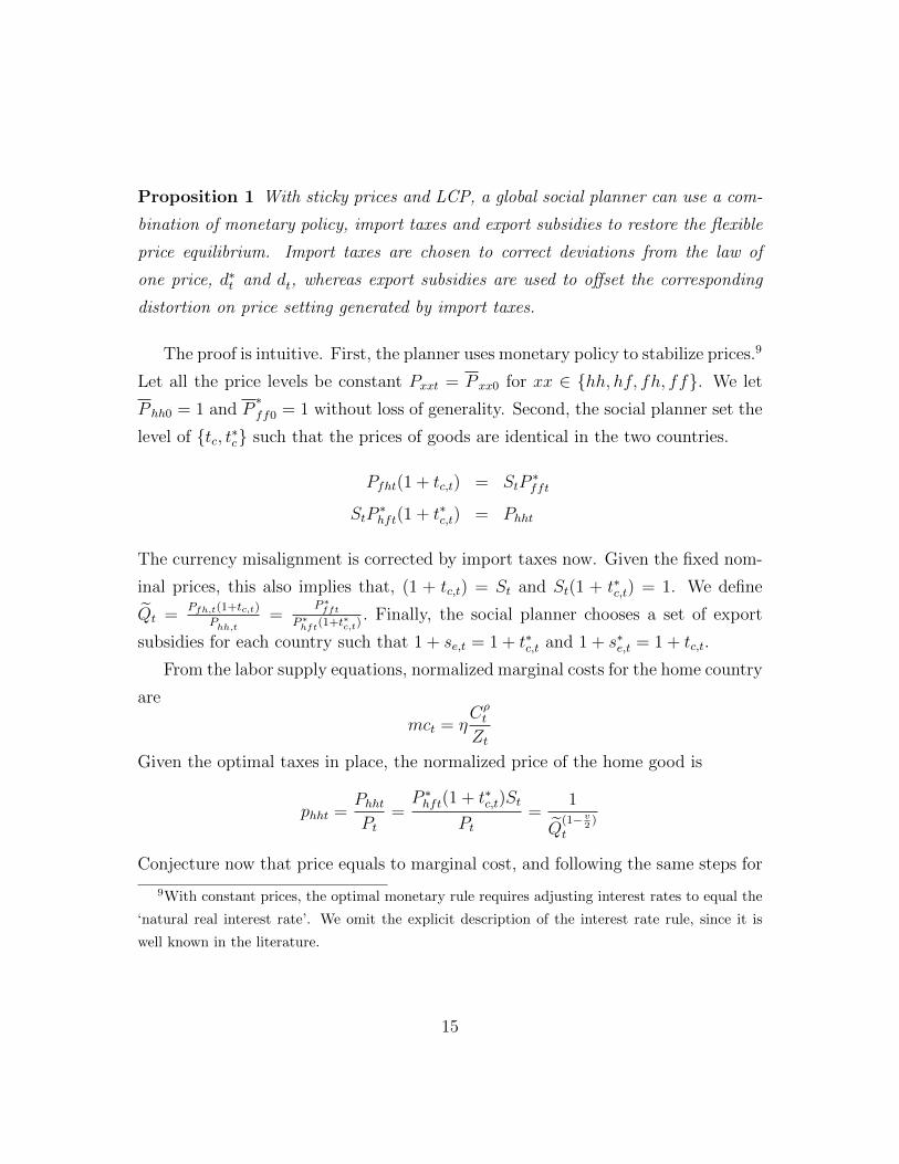
Proposition 1 With sticky prices and LCP, a global social planner can use a com-

bination of monetary policy, import taxes and export subsidies to restore the flexible

price equilibrium. Import taxes are chosen to correct deviations from the law of

one price, d∗t and dt, whereas export subsidies are used to offset the corresponding

distortion on price setting generated by import taxes.

The proof is intuitive. First, the planner uses monetary policy to stabilize prices.9

Let all the price levels be constant Pxxt = P xx0 for xx ∈ {hh, hf, fh, ff}. We let

P hh0 = 1 and P∗ff0 = 1 without loss of generality. Second, the social planner set the

level of {tc, t∗c} such that the prices of goods are identical in the two countries.

Pfht(1 + tc,t) = StP∗fft

StP∗hft(1 + t∗c,t) = Phht

The currency misalignment is corrected by import taxes now. Given the fixed nom-

inal prices, this also implies that, (1 + tc,t) = St and St(1 + t∗c,t) = 1. We define

Qt =Pfh,t(1+tc,t)

Phh,t=

P ∗fft

P ∗hft(1+t

∗c,t). Finally, the social planner chooses a set of export

subsidies for each country such that 1 + se,t = 1 + t∗c,t and 1 + s∗e,t = 1 + tc,t.

From the labor supply equations, normalized marginal costs for the home country

are

mct = ηCρt

Zt

Given the optimal taxes in place, the normalized price of the home good is

phht =PhhtPt

=P ∗hft(1 + t∗c,t)St

Pt=

1

Q(1− v

2)

t

Conjecture now that price equals to marginal cost, and following the same steps for

9With constant prices, the optimal monetary rule requires adjusting interest rates to equal the

‘natural real interest rate’. We omit the explicit description of the interest rate rule, since it is

well known in the literature.

15

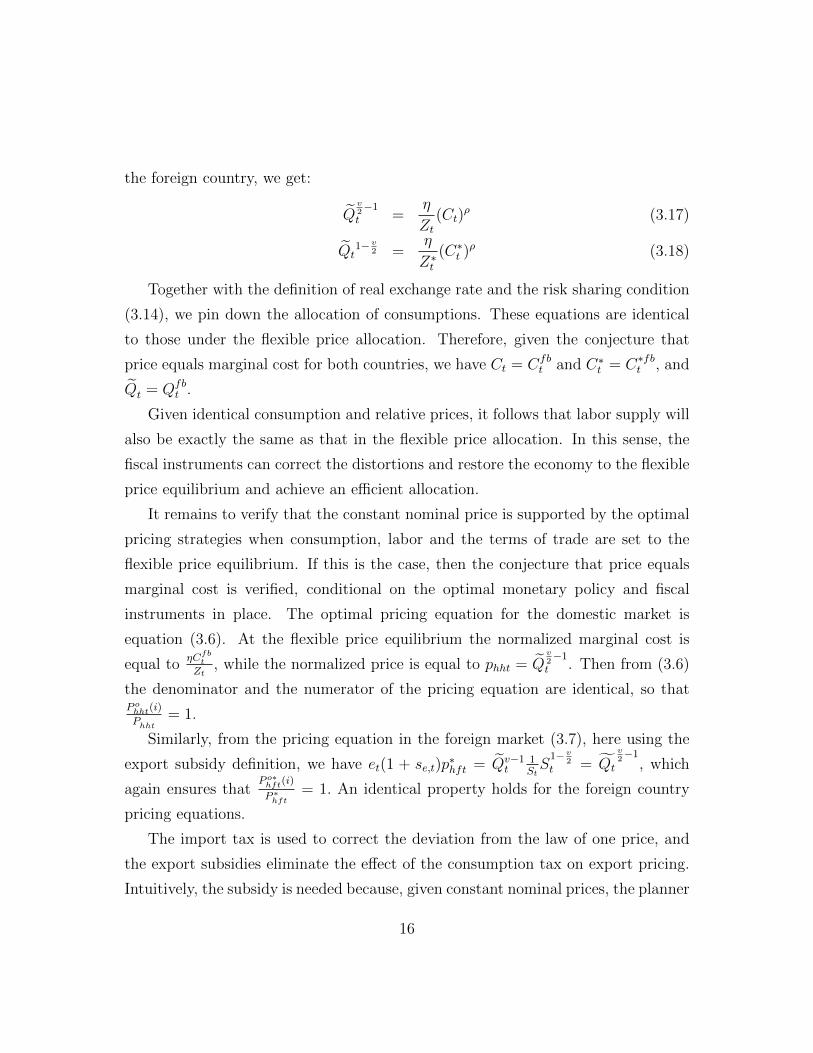
the foreign country, we get:

Qv2−1

t =η

Zt(Ct)

ρ (3.17)

Qt1− v

2 =η

Z∗t(C∗t )ρ (3.18)

Together with the definition of real exchange rate and the risk sharing condition

(3.14), we pin down the allocation of consumptions. These equations are identical

to those under the flexible price allocation. Therefore, given the conjecture that

price equals marginal cost for both countries, we have Ct = Cfbt and C∗t = C∗fbt , and

Qt = Qfbt .

Given identical consumption and relative prices, it follows that labor supply will

also be exactly the same as that in the flexible price allocation. In this sense, the

fiscal instruments can correct the distortions and restore the economy to the flexible

price equilibrium and achieve an efficient allocation.

It remains to verify that the constant nominal price is supported by the optimal

pricing strategies when consumption, labor and the terms of trade are set to the

flexible price equilibrium. If this is the case, then the conjecture that price equals

marginal cost is verified, conditional on the optimal monetary policy and fiscal

instruments in place. The optimal pricing equation for the domestic market is

equation (3.6). At the flexible price equilibrium the normalized marginal cost is

equal toηCfbtZt

, while the normalized price is equal to phht = Qv2−1

t . Then from (3.6)

the denominator and the numerator of the pricing equation are identical, so thatP ohht(i)

Phht= 1.

Similarly, from the pricing equation in the foreign market (3.7), here using the

export subsidy definition, we have et(1 + se,t)p∗hft = Qv−1

t1StS1− v

2t = Qt

v2−1

, which

again ensures thatP o∗hft(i)

P ∗hft

= 1. An identical property holds for the foreign country

pricing equations.

The import tax is used to correct the deviation from the law of one price, and

the export subsidies eliminate the effect of the consumption tax on export pricing.

Intuitively, the subsidy is needed because, given constant nominal prices, the planner

16

will need to adjust the nominal exchange rate to equal the efficient terms of trade.

Under LCP, the firm would want to adjust its foreign price in inverse proportion to

the nominal exchange rate, which lead to a deviation from the law of one price for

home and foreign sales of the home good. The export subsidy exactly offsets the

incentive for the home firm to do this.

Prices are constant over time, but the exchange rate is flexible, and import taxes

respond to the exchange rate to ensure efficient relative price adjustment for prices

facing households.10

Nominal wages will respond to productivity shocks and the allocation of con-

sumptions and labor is not distorted.

In summary, a combination of monetary and fiscal policy can support the fully

efficient allocation even when prices are set in local currency. Nevertheless, the

key question is how to implement these fiscal policy when there is no international

policy coordination. Below, we explore the implementation of the monetary and

fiscal policy in a non-cooperative environment.

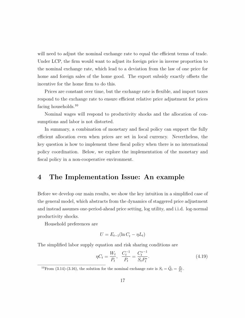
4 The Implementation Issue: An example

Before we develop our main results, we show the key intuition in a simplified case of

the general model, which abstracts from the dynamics of staggered price adjustment

and instead assumes one-period-ahead price setting, log utility, and i.i.d. log-normal

productivity shocks.

Household preferences are

U = Et−1(lnCt − ηLt)

The simplified labor supply equation and risk sharing conditions are

ηCt =Wt

Pt,C−1tPt

=C∗t−1

StP ∗t. (4.19)

10From (3.14)-(3.16), the solution for the nominal exchange rate is St = Qt = Zt

Z∗t

.

17

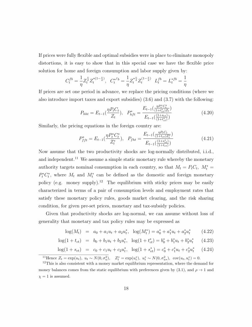
If prices were fully flexible and optimal subsidies were in place to eliminate monopoly

distortions, it is easy to show that in this special case we have the flexible price

solution for home and foreign consumption and labor supply given by:

Cfbt =

1

ηZ

v2t Z∗(1− v

2)

t , C∗f bt =

1

ηZ∗ v2

t Z(1− v

2)

t Lfbt = L∗fbt =1

η

If prices are set one period in advance, we replace the pricing conditions (where we

also introduce import taxes and export subsidies) (3.6) and (3.7) with the following:

Phht = Et−1(ηPtCtZt

), P ∗hft =Et−1(

ηP ∗t C

∗t

(1+t∗ct)Zt)

Et−1((1+set)(1+t∗ct)

)(4.20)

Similarly, the pricing equations in the foreign country are:

P ∗fft = Et−1(ηP ∗t C

∗t

Z∗t), Pfht =

Et−1(ηPtCt

(1+tct)Z∗t)

Et−1((1+s∗et)(1+tct)

)(4.21)

Now assume that the two productivity shocks are log-normally distributed, i.i.d.,

and independent.11 We assume a simple static monetary rule whereby the monetary

authority targets nominal consumption in each country, so that Mt = PtCt, M∗t =

P ∗t C∗t , where Mt and M∗

t can be defined as the domestic and foreign monetary

policy (e.g. money supply).12 The equilibrium with sticky prices may be easily

characterized in terms of a pair of consumption levels and employment rates that

satisfy these monetary policy rules, goods market clearing, and the risk sharing

condition, for given pre-set prices, monetary and tax-subsidy policies.

Given that productivity shocks are log-normal, we can assume without loss of

generality that monetary and tax policy rules may be expressed as

log(Mt) = a0 + a1ut + a2u∗t , log(M∗

t ) = a∗0 + a∗1ut + a∗2u∗t (4.22)

log(1 + tct) = b0 + b1ut + b2u∗t , log(1 + t∗ct) = b∗0 + b∗1ut + b∗2u

∗t (4.23)

log(1 + set) = c0 + c1ut + c2u∗t , log(1 + s∗et) = c∗0 + c∗1ut + c∗2u

∗t (4.24)

11Hence Zt = exp(ut), ut ∼ N(0, σ2u), Z∗t = exp(u∗t ), u

∗t ∼ N(0, σ2

u∗), cov(ut, u∗t ) = 0.

12This is also consistent with a money market equilibrium representation, where the demand for

money balances comes from the static equilibrium with preferences given by (3.1), and ρ→ 1 and

χ = 1 is assumed.

18

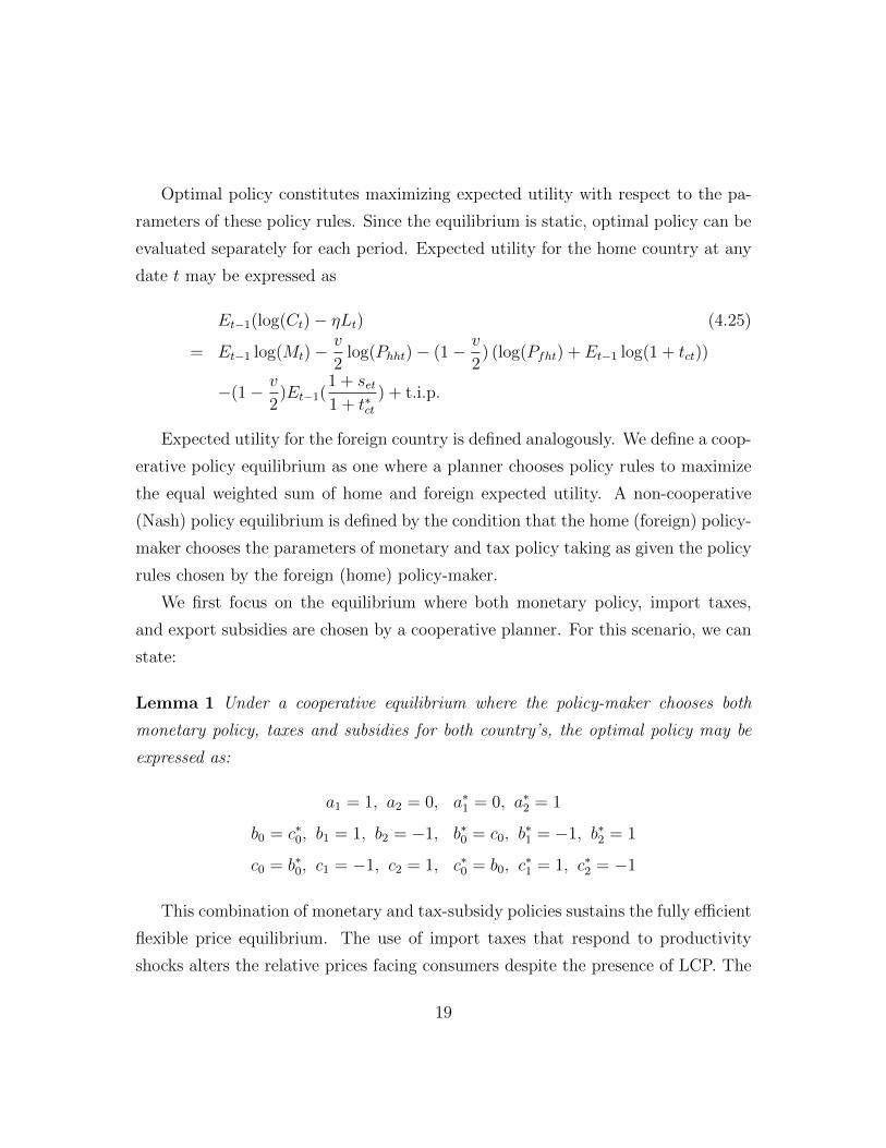
Optimal policy constitutes maximizing expected utility with respect to the pa-

rameters of these policy rules. Since the equilibrium is static, optimal policy can be

evaluated separately for each period. Expected utility for the home country at any

date t may be expressed as

Et−1(log(Ct)− ηLt) (4.25)

= Et−1 log(Mt)−v

2log(Phht)− (1− v

2) (log(Pfht) + Et−1 log(1 + tct))

−(1− v

2)Et−1(

1 + set1 + t∗ct

) + t.i.p.

Expected utility for the foreign country is defined analogously. We define a coop-

erative policy equilibrium as one where a planner chooses policy rules to maximize

the equal weighted sum of home and foreign expected utility. A non-cooperative

(Nash) policy equilibrium is defined by the condition that the home (foreign) policy-

maker chooses the parameters of monetary and tax policy taking as given the policy

rules chosen by the foreign (home) policy-maker.

We first focus on the equilibrium where both monetary policy, import taxes,

and export subsidies are chosen by a cooperative planner. For this scenario, we can

state:

Lemma 1 Under a cooperative equilibrium where the policy-maker chooses both

monetary policy, taxes and subsidies for both country’s, the optimal policy may be

expressed as:

a1 = 1, a2 = 0, a∗1 = 0, a∗2 = 1

b0 = c∗0, b1 = 1, b2 = −1, b∗0 = c0, b∗1 = −1, b∗2 = 1

c0 = b∗0, c1 = −1, c2 = 1, c∗0 = b0, c∗1 = 1, c∗2 = −1

This combination of monetary and tax-subsidy policies sustains the fully efficient

flexible price equilibrium. The use of import taxes that respond to productivity

shocks alters the relative prices facing consumers despite the presence of LCP. The

19

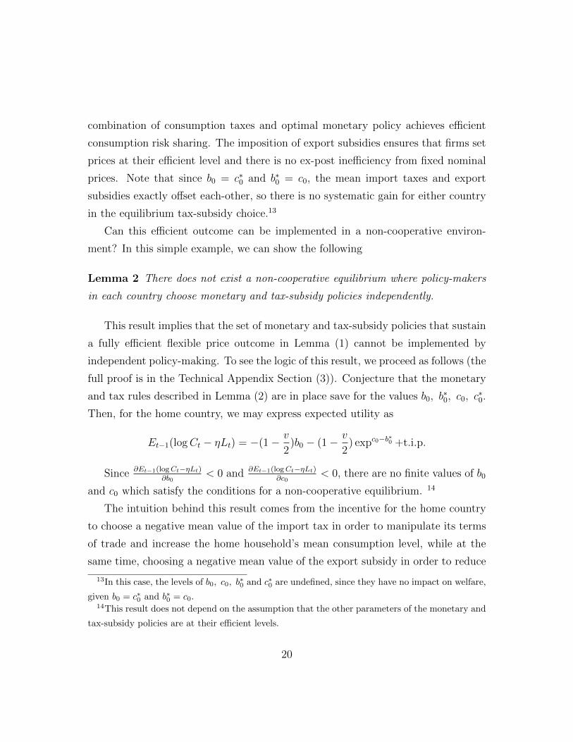
combination of consumption taxes and optimal monetary policy achieves efficient

consumption risk sharing. The imposition of export subsidies ensures that firms set

prices at their efficient level and there is no ex-post inefficiency from fixed nominal

prices. Note that since b0 = c∗0 and b∗0 = c0, the mean import taxes and export

subsidies exactly offset each-other, so there is no systematic gain for either country

in the equilibrium tax-subsidy choice.13

Can this efficient outcome can be implemented in a non-cooperative environ-

ment? In this simple example, we can show the following

Lemma 2 There does not exist a non-cooperative equilibrium where policy-makers

in each country choose monetary and tax-subsidy policies independently.

This result implies that the set of monetary and tax-subsidy policies that sustain

a fully efficient flexible price outcome in Lemma (1) cannot be implemented by

independent policy-making. To see the logic of this result, we proceed as follows (the

full proof is in the Technical Appendix Section (3)). Conjecture that the monetary

and tax rules described in Lemma (2) are in place save for the values b0, b∗0, c0, c

∗0.

Then, for the home country, we may express expected utility as

Et−1(logCt − ηLt) = −(1− v

2)b0 − (1− v

2) expc0−b

∗0 +t.i.p.

Since ∂Et−1(logCt−ηLt)∂b0

< 0 and ∂Et−1(logCt−ηLt)∂c0

< 0, there are no finite values of b0

and c0 which satisfy the conditions for a non-cooperative equilibrium. 14

The intuition behind this result comes from the incentive for the home country

to choose a negative mean value of the import tax in order to manipulate its terms

of trade and increase the home household’s mean consumption level, while at the

same time, choosing a negative mean value of the export subsidy in order to reduce

13In this case, the levels of b0, c0, b∗0 and c∗0 are undefined, since they have no impact on welfare,

given b0 = c∗0 and b∗0 = c0.14This result does not depend on the assumption that the other parameters of the monetary and

tax-subsidy policies are at their efficient levels.

20

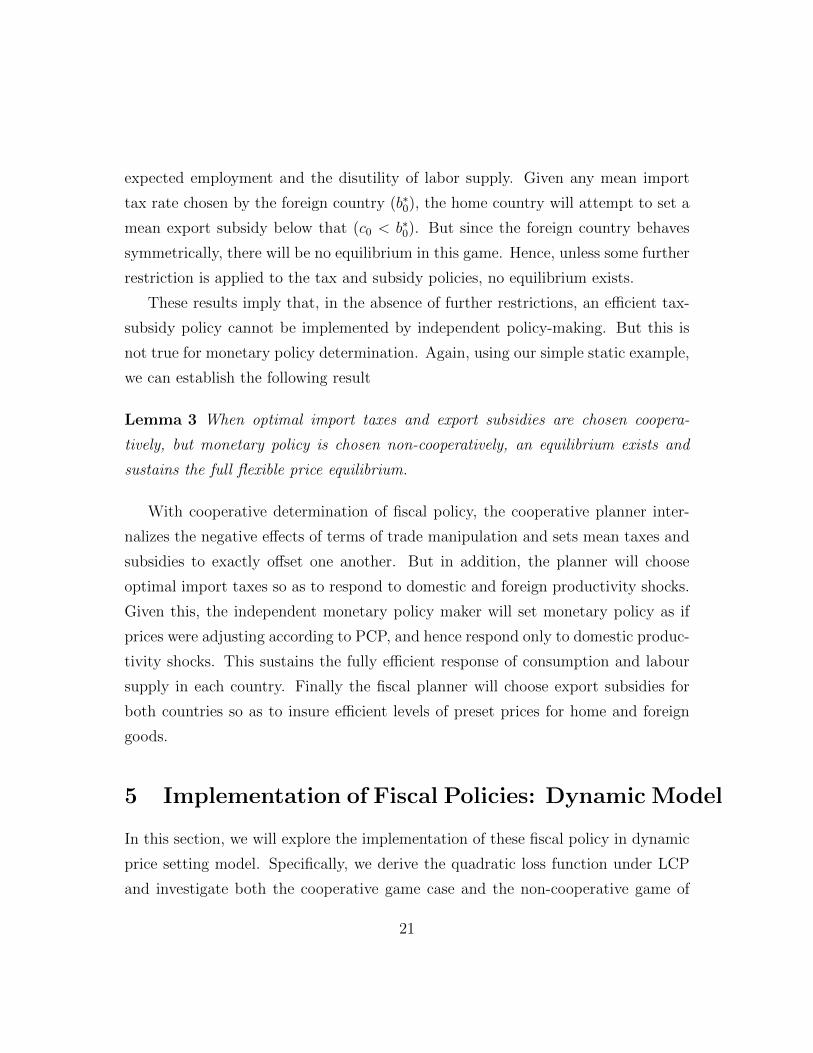
expected employment and the disutility of labor supply. Given any mean import

tax rate chosen by the foreign country (b∗0), the home country will attempt to set a

mean export subsidy below that (c0 < b∗0). But since the foreign country behaves

symmetrically, there will be no equilibrium in this game. Hence, unless some further

restriction is applied to the tax and subsidy policies, no equilibrium exists.

These results imply that, in the absence of further restrictions, an efficient tax-

subsidy policy cannot be implemented by independent policy-making. But this is

not true for monetary policy determination. Again, using our simple static example,

we can establish the following result

Lemma 3 When optimal import taxes and export subsidies are chosen coopera-

tively, but monetary policy is chosen non-cooperatively, an equilibrium exists and

sustains the full flexible price equilibrium.

With cooperative determination of fiscal policy, the cooperative planner inter-

nalizes the negative effects of terms of trade manipulation and sets mean taxes and

subsidies to exactly offset one another. But in addition, the planner will choose

optimal import taxes so as to respond to domestic and foreign productivity shocks.

Given this, the independent monetary policy maker will set monetary policy as if

prices were adjusting according to PCP, and hence respond only to domestic produc-

tivity shocks. This sustains the fully efficient response of consumption and labour

supply in each country. Finally the fiscal planner will choose export subsidies for

both countries so as to insure efficient levels of preset prices for home and foreign

goods.

5 Implementation of Fiscal Policies: Dynamic Model

In this section, we will explore the implementation of these fiscal policy in dynamic

price setting model. Specifically, we derive the quadratic loss function under LCP

and investigate both the cooperative game case and the non-cooperative game of

21

home and foreign fiscal and monetary policy authority. As illustrated in Section 3.4,

in Ramsey setting it is possible to use fiscal policy to replicate the efficient flexible

price equilibrium. So it is natural to use cooperative monetary and fiscal policy

game as a benchmark for the non-cooperative game. We will explore if the solution

to the international tax non-cooperative game exists. If not, then we ask what kind

of condition on the fiscal instruments is needed to ensure the existence of a Nash

international monetary and fiscal game and whether the solution to the Nash game

accord with that to the cooperative game.

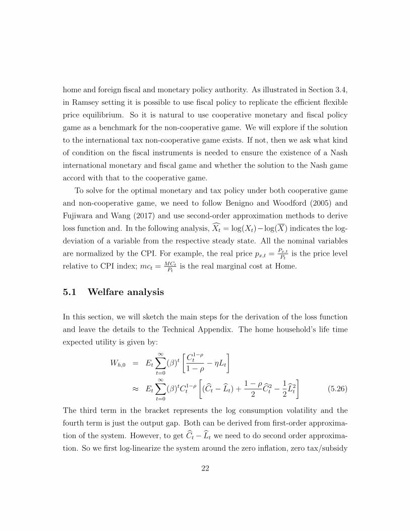
To solve for the optimal monetary and tax policy under both cooperative game

and non-cooperative game, we need to follow Benigno and Woodford (2005) and

Fujiwara and Wang (2017) and use second-order approximation methods to derive

loss function and. In the following analysis, Xt = log(Xt)− log(X) indicates the log-

deviation of a variable from the respective steady state. All the nominal variables

are normalized by the CPI. For example, the real price px,t = Px,tPt

is the price level

relative to CPI index; mct = MCtPt

is the real marginal cost at Home.

5.1 Welfare analysis

In this section, we will sketch the main steps for the derivation of the loss function

and leave the details to the Technical Appendix. The home household’s life time

expected utility is given by:

Wh,0 = Et

∞∑t=0

(β)t[C1−ρt

1− ρ− ηLt

]≈ Et

∞∑t=0

(β)tC1−ρt

[(Ct − Lt) +

1− ρ2

C2t −

1

2L2t

](5.26)

The third term in the bracket represents the log consumption volatility and the

fourth term is just the output gap. Both can be derived from first-order approxima-

tion of the system. However, to get Ct− Lt we need to do second order approxima-

tion. So we first log-linearize the system around the zero inflation, zero tax/subsidy

22

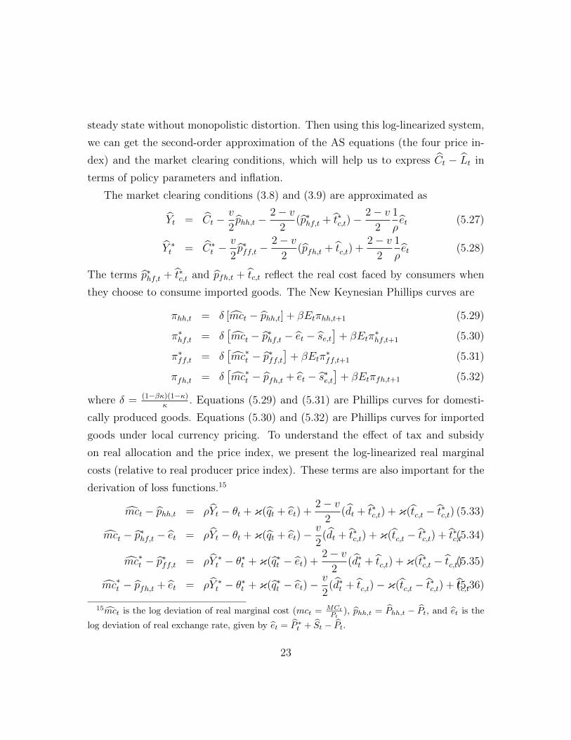
steady state without monopolistic distortion. Then using this log-linearized system,

we can get the second-order approximation of the AS equations (the four price in-

dex) and the market clearing conditions, which will help us to express Ct − Lt in

terms of policy parameters and inflation.

The market clearing conditions (3.8) and (3.9) are approximated as

Yt = Ct −v

2phh,t −

2− v2

(p∗hf,t + t∗c,t)−2− v

2

1

ρet (5.27)

Y ∗t = C∗t −v

2p∗ff,t −

2− v2

(pfh,t + tc,t) +2− v

2

1

ρet (5.28)

The terms p∗hf,t + t∗c,t and pfh,t + tc,t reflect the real cost faced by consumers when

they choose to consume imported goods. The New Keynesian Phillips curves are

πhh,t = δ [mct − phh,t] + βEtπhh,t+1 (5.29)

π∗hf,t = δ[mct − p∗hf,t − et − se,t

]+ βEtπ

∗hf,t+1 (5.30)

π∗ff,t = δ[mc∗t − p∗ff,t

]+ βEtπ

∗ff,t+1 (5.31)

πfh,t = δ[mc∗t − pfh,t + et − s∗e,t

]+ βEtπfh,t+1 (5.32)

where δ = (1−βκ)(1−κ)κ

. Equations (5.29) and (5.31) are Phillips curves for domesti-

cally produced goods. Equations (5.30) and (5.32) are Phillips curves for imported

goods under local currency pricing. To understand the effect of tax and subsidy

on real allocation and the price index, we present the log-linearized real marginal

costs (relative to real producer price index). These terms are also important for the

derivation of loss functions.15

mct − phh,t = ρYt − θt + κ(qt + et) +2− v

2(dt + t∗c,t) + κ(tc,t − t∗c,t) (5.33)

mct − p∗hf,t − et = ρYt − θt + κ(qt + et)−v

2(dt + t∗c,t) + κ(tc,t − t∗c,t) + t∗c,t(5.34)

mc∗t − p∗ff,t = ρY ∗t − θ∗t + κ(q∗t − et) +2− v

2(d∗t + tc,t) + κ(t∗c,t − tc,t)(5.35)

mc∗t − pfh,t + et = ρY ∗t − θ∗t + κ(q∗t − et)−v

2(d∗t + tc,t)− κ(tc,t − t∗c,t) + tc,t(5.36)

15mct is the log deviation of real marginal cost (mct = MCt

Pt), phh,t = Phh,t − Pt, and et is the

log deviation of real exchange rate, given by et = P ∗t + St − Pt.

23

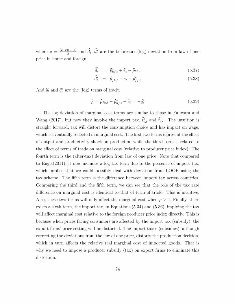
where κ = (2−v)(1−ρ)2

and dt, d∗t are the before-tax (log) deviation from law of one

price in home and foreign.

dt = p∗hf,t + et − phh,t (5.37)

d∗t = pfh,t − et − p∗ff,t (5.38)

And qt and q∗t are the (log) terms of trade.

qt = pfh,t − p∗hf,t − et = −q∗t (5.39)

The log deviation of marginal cost terms are similar to those in Fujiwara and

Wang (2017), but now they involve the import tax, t∗c,t and tc,t. The intuition is

straight forward, tax will distort the consumption choice and has impact on wage,

which is eventually reflected in marginal cost. The first two terms represent the effect

of output and productivity shock on production while the third term is related to

the effect of terms of trade on marginal cost (relative to producer price index). The

fourth term is the (after-tax) deviation from law of one price. Note that compared

to Engel(2011), it now includes a log tax term due to the presence of import tax,

which implies that we could possibly deal with deviation from LOOP using the

tax scheme. The fifth term is the difference between import tax across countries.

Comparing the third and the fifth term, we can see that the role of the tax rate

difference on marginal cost is identical to that of term of trade. This is intuitive.

Also, these two terms will only affect the marginal cost when ρ > 1. Finally, there

exists a sixth term, the import tax, in Equations (5.34) and (5.36), implying the tax

will affect marginal cost relative to the foreign producer price index directly. This is

because when prices facing consumers are affected by the import tax (subsidy), the

export firms’ price setting will be distorted. The import taxes (subsidies), although

correcting the deviations from the law of one price, distorts the production decision,

which in turn affects the relative real marginal cost of imported goods. That is

why we need to impose a producer subsidy (tax) on export firms to eliminate this

distortion.

24

In the following analysis, we will first derive the global loss function with tax and

subsidy for the cooperative game. We check if these fiscal instruments can correct

the welfare loss due to deviation from LOOP and help to achieve the flexible price

equilibrium. Note that in the dynamic model, the most desirable level to which

monetary policy can deliver is the flexible price equilibrium level, which will be

used as a target for international tax policies. Since we remove the monopolistic

competition by a constant tax, it is also the efficient equilibrium, as that in Fujiwara

and Wang (2017).

5.2 Cooperative Game

As discussed in Clarida, Gali and Gertler (2002), the terms of trade effect and the

risk-sharing effect cancel out with each other when ρ = 1, which greatly simplifies

the expression for the loss function. Since the effect of currency misalignment on

marginal cost does not depend on whether ρ is greater, smaller, or equal to 1, we

will look at the ρ = 1 first to simplify our analysis. The case with ρ > 1 will be

discussed later. Countries are assumed to have equal size, so the global welfare

loss in the cooperative game is L0 = Lh,0 + L∗h,0, where Lh,0 and L∗h,0 are the loss

functions for the home and foreign countries, respectively.

5.2.1 The Cooperative Game when ρ = 1

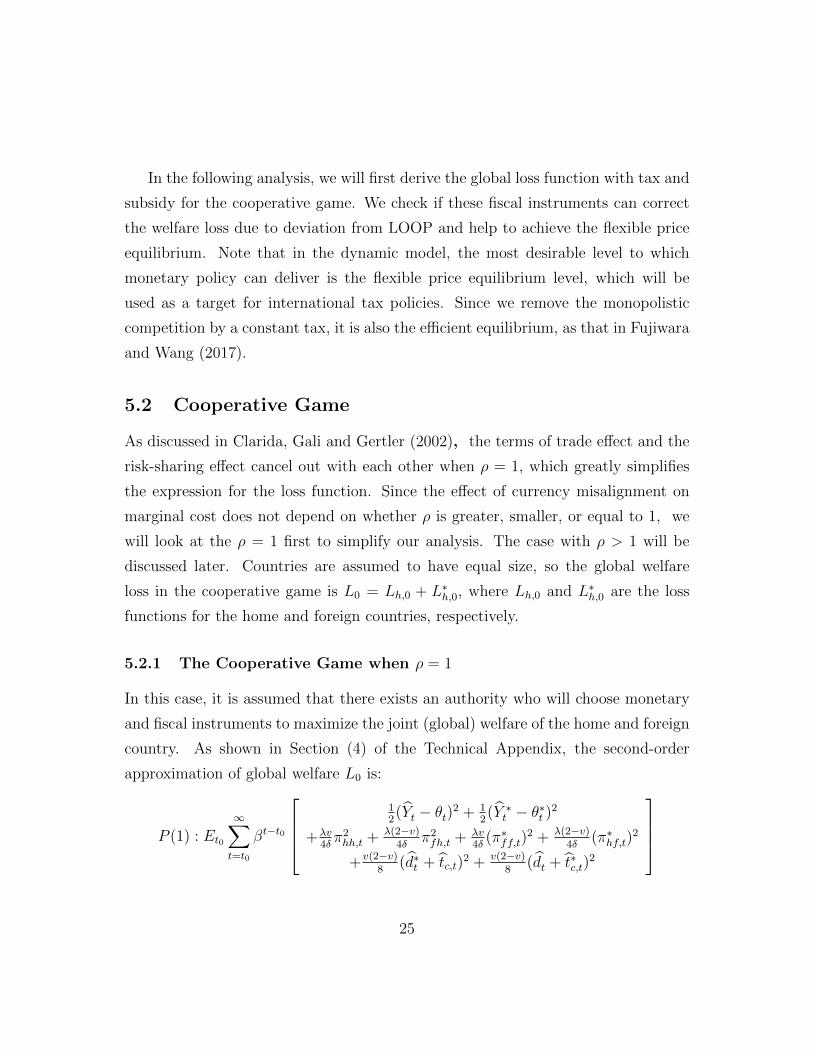
In this case, it is assumed that there exists an authority who will choose monetary

and fiscal instruments to maximize the joint (global) welfare of the home and foreign

country. As shown in Section (4) of the Technical Appendix, the second-order

approximation of global welfare L0 is:

P (1) : Et0

∞∑t=t0

βt−t0

12(Yt − θt)2 + 1

2(Y ∗t − θ∗t )2

+λv4δπ2hh,t + λ(2−v)

4δπ2fh,t + λv

4δ(π∗ff,t)

2 + λ(2−v)4δ

(π∗hf,t)2

+v(2−v)8

(d∗t + tc,t)2 + v(2−v)

8(dt + t∗c,t)

2

25

The first two terms are quadratic deviation from steady state output. The

following four terms represent squared inflation rate of local as well as imported

products, which capture price dispersions. For example, πhh,t = πt+ phh,t− phh,t−1 is

the deviation of inflation of home goods sold in home from the steady state (πhh = 0),

and the other terms are defined analogously. The last two terms are related to the

welfare loss due to deviations from law of one price (LOOP). Interestingly, if there are

not tax policies, then the last two terms will become v(2−v)8

(d∗t )2+ v(2−v)

8(dt)

2. This is

exactly the currency misalignment problem emphasized in Engel(2011). Comparing

to that in Engel (2011) and Fujiwara and Wang(2017), in our model with fiscal

instruments, they show up in the loss function together with the import tax. As

in Clarida, Gali and Gertler (2002), since we assume ρ = 1, terms of trade qt =

pfh,t − et − p∗hf,t will not appear in the loss function.

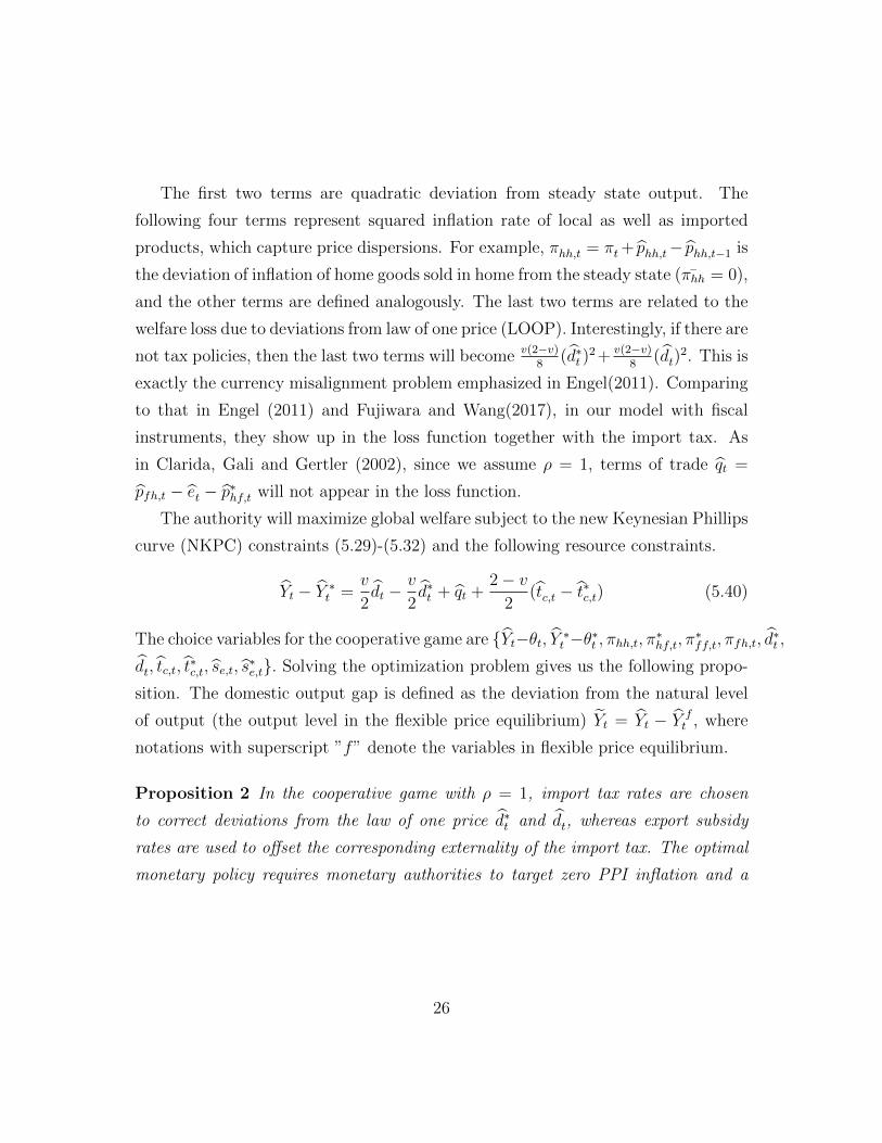
The authority will maximize global welfare subject to the new Keynesian Phillips

curve (NKPC) constraints (5.29)-(5.32) and the following resource constraints.

Yt − Y ∗t =v

2dt −

v

2d∗t + qt +

2− v2

(tc,t − t∗c,t) (5.40)

The choice variables for the cooperative game are {Yt−θt, Y ∗t −θ∗t , πhh,t, π∗hf,t, π∗ff,t, πfh,t, d∗t ,dt, tc,t, t

∗c,t, se,t, s

∗e,t}. Solving the optimization problem gives us the following propo-

sition. The domestic output gap is defined as the deviation from the natural level

of output (the output level in the flexible price equilibrium) Yt = Yt − Y ft , where

notations with superscript ”f” denote the variables in flexible price equilibrium.

Proposition 2 In the cooperative game with ρ = 1, import tax rates are chosen

to correct deviations from the law of one price d∗t and dt, whereas export subsidy

rates are used to offset the corresponding externality of the import tax. The optimal

monetary policy requires monetary authorities to target zero PPI inflation and a

26

zero output gap.

Yt = Yt∗

= 0

Yt = Y ft = θt, Y

∗t = Y ∗ft = θ∗t

−dt = t∗c,t = se,t, − d∗t = tc,t = s∗e,t

πhh,t = 0, π∗ff,t = 0, π∗hf,t = 0, πfh,t = 0

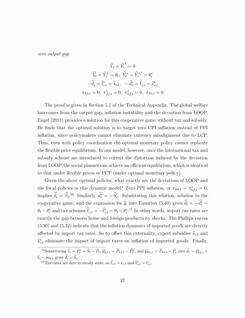
The proof is given in Section 5.1 of the Technical Appendix. The global welfare

loss comes from the output gap, inflation instability and the deviation from LOOP.

Engel (2011) provides a solution for this cooperative game without tax and subsidy.

He finds that the optimal solution is to target zero CPI inflation instead of PPI

inflation, since policymakers cannot eliminate currency misalignment due to LCP.

Thus, even with policy coordination the optimal monetary policy cannot replicate

the flexible price equilibrium. In our model, however, once the international tax and

subsidy scheme are introduced to correct the distortion induced by the deviation

from LOOP, the social planner can achieve an efficient equilibrium, which is identical

to that under flexible prices or PCP (under optimal monetary policy).

Given the above optimal policies, what exactly are the deviations of LOOP and

the fiscal policies in this dynamic model? Zero PPI inflation, or πhh,t = π∗hf,t = 0,

implies dt = St.16 Similarly, d∗t = −St. Substituting this relation, solution to the

cooperative game, and the expression for qt into Equation (5.40) gives dt = −d∗t =

θt− θ∗t and tax schemes tc,t = −t∗c,t = θt− θ∗t .17 In other words, import tax rates are

exactly the gap between home and foreign productivity shocks. The Phillips curves

(5.30) and (5.32) indicate that the inflation dynamics of imported goods are directly

affected by import tax rates. So to offset this externality, export subsidies se,t and

s∗e,t eliminate the impact of import taxes on inflation of imported goods. Finally,

16Substituting et = P ∗t + St − Pt, p∗hf,t = Phf,t − P ∗t , and phh,t = Phh,t − Pt into dt = p∗hf,t +

et − phh,t gives dt = St.17Tax rates are zero in steady state, so tc,t = tc,t and t∗c,t = t∗c,t.

27

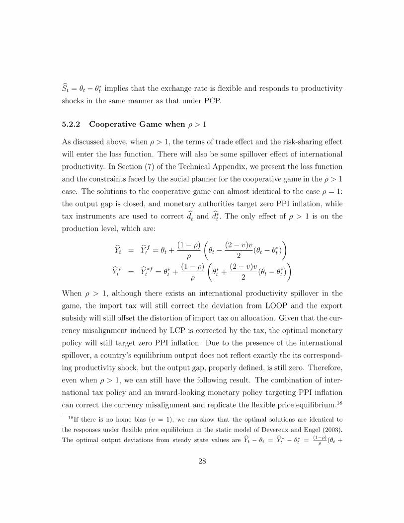
St = θt − θ∗t implies that the exchange rate is flexible and responds to productivity

shocks in the same manner as that under PCP.

5.2.2 Cooperative Game when ρ > 1

As discussed above, when ρ > 1, the terms of trade effect and the risk-sharing effect

will enter the loss function. There will also be some spillover effect of international

productivity. In Section (7) of the Technical Appendix, we present the loss function

and the constraints faced by the social planner for the cooperative game in the ρ > 1

case. The solutions to the cooperative game can almost identical to the case ρ = 1:

the output gap is closed, and monetary authorities target zero PPI inflation, while

tax instruments are used to correct dt and d∗t . The only effect of ρ > 1 is on the

production level, which are:

Yt = Y ft = θt +

(1− ρ)

ρ

(θt −

(2− v)v

2(θt − θ∗t )

)Y ∗t = Y ∗ft = θ∗t +

(1− ρ)

ρ

(θ∗t +

(2− v)v

2(θt − θ∗t )

)When ρ > 1, although there exists an international productivity spillover in the

game, the import tax will still correct the deviation from LOOP and the export

subsidy will still offset the distortion of import tax on allocation. Given that the cur-

rency misalignment induced by LCP is corrected by the tax, the optimal monetary

policy will still target zero PPI inflation. Due to the presence of the international

spillover, a country’s equilibrium output does not reflect exactly the its correspond-

ing productivity shock, but the output gap, properly defined, is still zero. Therefore,

even when ρ > 1, we can still have the following result. The combination of inter-

national tax policy and an inward-looking monetary policy targeting PPI inflation

can correct the currency misalignment and replicate the flexible price equilibrium.18

18If there is no home bias (υ = 1), we can show that the optimal solutions are identical to

the responses under flexible price equilibrium in the static model of Devereux and Engel (2003).

The optimal output deviations from steady state values are Yt − θt = Y ∗t − θ∗t = (1−ρ)ρ (θt +

28

Having shown that these fiscal instruments can correct the currency misalign-

ment due to LCP and deliver the flexible price equilibrium under the cooperative

game, the next step is to explore the implementation of these international fiscal

policies in non-cooperative environment.

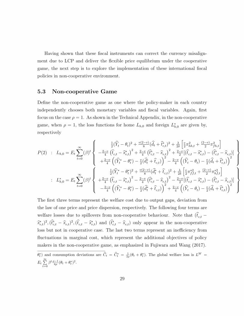
5.3 Non-cooperative Game

Define the non-cooperative game as one where the policy-maker in each country

independently chooses both monetary variables and fiscal variables. Again, first

focus on the case ρ = 1. As shown in the Technical Appendix, in the non-cooperative

game, when ρ = 1, the loss functions for home Lh,0 and foreign L∗h,0 are given by,

respectively

P (2) : Lh,0 = Et

∞∑t=0

(β)t

12(Yt − θt)2 + v(2−v)

8(dt + t∗c,t)

2 + λ2δ

[v2π2hh,t + (2−v)

2π2fh,t

]−2−v

4

(tc,t − s∗e,t

)2+ 2−v

4

(t∗c,t − se,t

)2+ 2−v

2[(tc,t − s∗e,t)− (t∗c,t − se,t)]

+2−v4

((Y ∗t − θ∗t )− v

2(d∗t + tc,t)

)2− 2−v

4

((Yt − θt)− v

2(dt + t∗c,t)

)2

: L∗h,0 = Et

∞∑t=0

(β)t

12(Y ∗t − θ∗t )2 + v(2−v)

8(d∗t + tc,t)

2 + λ2δ

[v2π∗2ff,t + (2−v)

2π∗2hf,t

]+2−v

4

(tc,t − s∗e,t

)2 − 2−v4

(t∗c,t − se,t

)2 − 2−v2

[(tc,t − s∗e,t)− (t∗c,t − se,t)]

−2−v4

((Y ∗t − θ∗t )− v

2(d∗t + tc,t)

)2+ 2−v

4

((Yt − θt)− v

2(dt + t∗c,t)

)2

The first three terms represent the welfare cost due to output gaps, deviation from

the law of one price and price dispersion, respectively. The following four terms are

welfare losses due to spillovers from non-cooperative behaviour. Note that (tc,t −s∗e,t)

2, (t∗c,t − se,t)2, (tc,t − s∗e,t) and (t∗c,t − se,t) only appear in the non-cooperative

loss but not in cooperative case. The last two terms represent an inefficiency from

fluctuations in marginal cost, which represent the additional objectives of policy

makers in the non-cooperative game, as emphasized in Fujiwara and Wang (2017).

θ∗t ) and consumption deviations are Ct = C∗t = 12ρ (θt + θ∗t ). The global welfare loss is LW =

Et∞∑t=0

βt ρ−14ρ (θt + θ∗t )2.

29

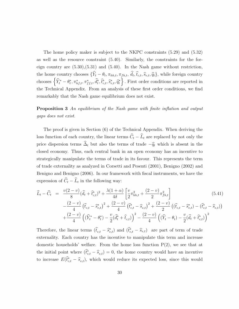
The home policy maker is subject to the NKPC constraints (5.29) and (5.32)

as well as the resource constraint (5.40). Similarly, the constraints for the for-

eign country are (5.30),(5.31) and (5.40). In the Nash game without restriction,

the home country chooses {Yt − θt, πhh,t, πfh,t, dt, tc,t, se,t, qt}, while foreign country

chooses{Y ∗t − θ∗t , π∗hf,t, π∗ff,t, d∗t , t∗c,t, s∗e,t, q∗t

}. First order conditions are reported in

the Technical Appendix. From an analysis of these first order conditions, we find

remarkably that the Nash game equilibrium does not exist.

Proposition 3 An equilibrium of the Nash game with finite inflation and output

gaps does not exist.

The proof is given in Section (6) of the Technical Appendix. When deriving the

loss function of each country, the linear terms Ct − Lt are replaced by not only the

price dispersion terms ∆t but also the terms of trade −qt which is absent in the

closed economy. Thus, each central bank in an open economy has an incentive to

strategically manipulate the terms of trade in its favour. This represents the term

of trade externality as analyzed in Corsetti and Pesenti (2001), Benigno (2002) and

Benigno and Benigno (2006). In our framework with fiscal instruments, we have the

expression of Ct − Lt in the following way:

Lt − Ct =v(2− v)

8(dt + t∗c,t)

2 +λ(1 + α)

4δ

[v

2π2hh,t +

(2− v)

2π2fh,t

](5.41)

−(2− v)

4

(tc,t − s∗e,t

)2+

(2− v)

4

(t∗c,t − se,t

)2+

(2− v)

2

((tc,t − s∗e,t)− (t∗c,t − se,t)

)+

(2− v)

4

((Y ∗t − θ∗t )−

v

2(d∗t + tc,t)

)2− (2− v)

4

((Yt − θt)−

v

2(dt + t∗c,t)

)2Therefore, the linear terms (tc,t − s∗e,t) and (t∗c,t − se,t) are part of term of trade

externality. Each country has the incentive to manipulate this term and increase

domestic households’ welfare. From the home loss function P(2), we see that at

the initial point where (t∗c,t − se,t) = 0, the home country would have an incentive

to increase E(t∗c,t − se,t), which would reduce its expected loss, since this would

30

raise its expected terms of trade. This is reflected in the first order condition under

noncooperative behaviour when the government chooses the optimal subsidy se,t.

−(2− v)

2

(t∗c,t − se,t

)+

(2− v)

2= 0 (5.42)

So the home government would wish to have E(t∗c,t − se,t) > 0. But from (??),

at Y ∗t − θ∗t = 0 and d∗t + tc,t = 0, this would imply that πfh,t cannot converge to

zero, even in the absence of productivity shocks. In fact, as shown in the technical

appendix, any solution to the non-cooperative game must have πfh,t diverging to

infinity. Therefore, there is no equilibrium with finite inflation rates. As a result

there is a fundamental inconsistency between the policymakers goal of inflation

control and the desire to exploit its terms of trade advantage in the non-cooperative

game where each policymaker has responsibility for both monetary policy and fiscal

instruments.

5.4 Implementability in a Three-player Nash Game

Is there any restriction that could help to regain the Nash equilibrium? Obviously,

from the analysis above, one natural restriction would be se,t = t∗c,t and s∗e,t = tc,t. By

artificially imposing a restriction on tax policy such that the home import tax exactly

equals the export subsidy for foreign exporters, the terms of trade externality due

to international tax competition externality can be avoided. After this restriction is

imposed, there will be a solution to the restricted Nash game and it replicates the

flexible price equilibrium.

Proposition 4 With the restriction that t∗c,t = se,t and tc,t = s∗e,t, the non-cooperative

equilibrium exists. It also replicates the flexible equilibrium. That is, the solutions

to the restricted Nash game are the same as those in the cooperative game.

Proofs are given in Section (6) of the Technical Appendix. Thus, we conclude

that even under the non-cooperative game, the international tax policy combined

31

with the import tax and export subsidy can be used to replicate the flexible price

equilibrium and improve global welfare.

How can this condition be rationalized? We now define a mixed environment

where there is coordination in fiscal policy but non-cooperative monetary policy.

To achieve this goal, we distinguish between fiscal authorities and monetary

authorities. Instead of assuming that the monetary authorities choose the level

of tax or subsidies, we assume that they take the tax and subsidies policy rules

as given, but choose inflation and output gaps independently (non-cooperatively).

Meanwhile, the fiscal authorities choose the optimal responses of tax and subsidies.

But to avoid the terms of trade externality in the choice of fiscal instruments, fiscal

policies must be chosen cooperatively. Hence, we define a 3 player Nash game, where

there are two monetary authorities and a global fiscal alliance.

The objective functions and constraints of the home and foreign monetary au-

thorities are identical to the problem characterized by P(2), the only difference is

that{tc,t, se,t

}and

{t∗c,t, s

∗e,t

}are not their choice variables. The objective function

of global fiscal authorities, as well as the constraint, is identical to the problem

characterized by P(1) but they can only choose the tax and subsidies instruments.

Proposition 5 The solution to the 3 player Nash game is the same as those in the

cooperative game. In other words, effective fiscal policy coordination in tax policies

among governments is necessary for non-cooperative ( or self-oriented) monetary

policy to sustain an efficient outcome.

Proofs are given the Technical Appendix. Intuitively, fiscal authorities can use

the import tax to correct the welfare costs due to currency misalignment and ensure

that this import tax will not affect the inflation rate, by using export subsidies. The

governments can implement this fiscal scheme without coordinating with the mone-

tary authorities. In effect, coordination between fiscal authorities is more desirable

than coordination between monetary authorities, from the perspective of correcting

32

currency misalignment.19

Clarida, Gali and Gertler (2002) show that when ρ = 1, there is no gain from

policy coordination under PCP framework. In our model, once the deviation of the

law of one price due to LCP is corrected by the international tax coordination there

is no extra gain from monetary policy coordination. This implication differs from

Fujiwara and Wang (2017), where they find that there is some policy coordination

gain from monetary policy coordination under LCP. This is because, in our model,

once the currency misalignment is corrected, the optimal monetary policy can

again target producer price stability, as in the case of PCP. Therefore, the optimal

monetary and fiscal policy mix delivers the same results under both the cooperative

game and non-cooperative game, which is the flexible price equilibrium under PCP.

In our model, the key policy coordination gain is from the fiscal policy coordination.

We discuss this in Section 7, where we define the welfare gain as the difference

between welfare under the LCP case without fiscal policy and the flexible price

equilibrium.

5.4.1 ρ > 1 case

We also check if the results discussed above hold when ρ > 1. Section (8) and (9) of

the Technical Appendix give the loss function and constraints faced by players for

the restricted Nash game and for the three-player Nash game. We show that both

Nash games deliver exactly the same solution as that in the cooperative game. The

proof is given in the Technical Appendix. This implies that for a more general setup,

we can still show that the combination of monetary policy and state-contingent taxes

and subsidies can be used to eliminate the inefficiency caused by LCP and replicate

the flexible price equilibrium.

19We note again that fiscal policy to deal with the welfare loss due to local currency pricing is

also proposed by Adao, Correia, and Teles (2009). The key difference here however it that optimal

tax policy is derived from three-player Nash game among coordinated fiscal alliance, home and

foreign money authorities.

33

In summary, we show that even under the non-cooperative Nash game, a state-

contingent tax policy combination of import tax (subsidy) and export subsidy (tax)

can fully correct the currency misalignment due to LCP. But critically, this requires

coordination in fiscal policy. The independent determination of taxes and subsidies,

while allowing policymakers to eliminate currency misalignment, opens up a new

strategic channel through the terms of trade externality which, as we have shown,

is inconsistent with the desire to eliminate output gaps and achieve zero inflation.

6 Discussion of Other Tax Instruments

In this subsection, we introduce some other tax instruments discussed in the litera-

ture. In particular, we allow for a labor income tax and a consumption tax on both

home and foreign goods. The model specification is similar to the benchmark dy-

namic model, so we only list a few key equations which change when these additional

tax instruments are considered. 20

The amended household budget constraint now becomes:

(1 + th,t)PhhtCh,t + (1 + tf,t)PfhtCf,t +Mt+1 +Bht+1 +∑

ζt+1∈Zt+1

B(ζt+1|ζt)D(ζt+1)

= (1− τt)WtLt +Rt−1Bht + Πt +Mt + Tt +D(ζt) (6.43)

where th,t and tf,t are the import tax on home and foreign goods, respectively;

and τt is the labor income tax. The labor supply curve becomes:

(1− τt)WtC−ρtPt

= η (6.44)

20The instruments here are the same as those used in used in Adao, Correia, and Teles (2009),

although some key features of the market structure differ. They show that a labor income tax and

consumption taxes on both home goods and foreign goods can be used to replicate the flexible

price equilibrium. And given these taxes, they find that the exchange rate regime and the currency

of pricing is irrelevant. But since we assume complete risk sharing, our setting differs from theirs

in terms of asset market completeness.

34

Demand for home and foreign goods are now given by:

Ch,t =v

2

PtCtPhht(1 + th,t)

(6.45)

Cf,t = (1− v

2)

PtCtPfht(1 + tf,t)

(6.46)

Note that firms’ pricing equations are now the same as those in the standard

literature since export subsidies are no longer considered.

Finally, the home market clearing condition is

Yt =v

2

PtCtPhht(1 + th,t)

∆hh,t + (1− v

2)

P ∗t C∗t

P ∗hft(1 + t∗h,t)∆∗hf,t (6.47)

The foreign counterparts are defined analogously. We then check if these instru-

ments can replicate the flexible price equilibrium. For simplicity and the purpose

of comparison, we focus on the case where ρ = 1. We first look at the coopera-

tive game. As shown in the Technical Appendix Section (10), the solution to the

cooperative game is as follows:

πhh,t = π∗hf,t = π∗ff,t = πfh,t = 0

Yt − θt = 0; Y ∗t − θ∗t = 0

th,t = t∗h,t = −τttf,t = t∗f,t = −τ ∗td∗t = dt = St = 0

This solution indeed establishes that the flexible price equilibrium can be achieved

using these instruments under a cooperative game. This is consistent with Adao,

Correa and Teles (2009), although we have a different international financial market

structure in our model. However, two things should be noted. First, the level of the

home and foreign labor income tax is indeterminate. The need to eliminate currency

misalignment requires for instance that dt + t∗h,t − th,t = 0 and th,t + τt = 0, but

we cannot uniquely pin down the individual tax rates. Both home and foreign con-

sumers are subject to the same tax responses on home goods, and similarly for the

35

tax responses on foreign goods. The labor income tax is used to offset the supply ef-

fects of the tax rates, similar to the role of the export subsidy in our previous model.

But what matters in terms of adjusting relative demand efficiently is the difference

between the tax on home goods and that on foreign goods, not the individual tax

rates.

Second, the exchange rate has to be fixed. Once the responses of taxes on home

and foreign goods have been put in place, nominal prices do not move, and since

the taxes respond identically for both home and foreign consumers, any movement

in the exchange rate would in fact generate a deviation from the law of one price.

To eliminate this, we require the exchange rate to be fixed.

We then explore if the flexible price equilibrium can be supported in the non-

cooperative Nash game. As discussed in Section 10.1 of the Technical Appendix, it

cannot. In fact, there does not exist a solution to the Nash equilibrium. The deriva-

tion of the non-existence condition is very similar to that in our main benchmark

model. Like in the benchmark model with import tax and export subsidy, in the

home and foreign loss function there exist linear terms of labor income taxes and

consumption taxes. Intuitively, individual authorities would wish to have a non-zero

expected labor tax to manipulate terms of trade, which leads to no finite equilib-

rium level of inflation and non-existence of Nash equilibrium. Hence, as in our main

model, these instruments cannot be used to replicate the flexible price equilibrium

in a non-cooperative fiscal policy game. Some further restrictions or international

coordination would be needed.

7 Quantitative Welfare Gain

In this section, we give a quantitative evaluation of the gains to employing state

contingent fiscal policies to correct currency misalignment. We can define the wel-

fare gain as the welfare achieved under the fully efficient allocation (which can be

supported under the 3 player Nash game), relative to the welfare under a non-

36

cooperative monetary policy equilibrium, without the use of fiscal policies. This

latter equilibrium is that analyzed by Fujiwara and Wang (2017).

As shown above, when optimal, state-contingent fiscal policies are used, the

economy can achieve the fully efficient allocations. Hence, from one perspective, the

welfare loss of currency misalignment in Engel (2011), which cannot be eliminated by

the optimal monetary policy (CPI targeting in his paper), can be taken as the welfare

improvement of our policy mix, relative to the optimal cooperative monetary policy

derived in Engel (2011). To obtain a quantitative welfare improvement, we conduct

a simple exercise to compare the welfare gain (in terms of steady state consumption)

under the cooperative monetary policy and that in the flexible price equilibrium.

All parameters are documented in Table 2 and identical to that in Engel (2011).

The welfare loss under the efficient, flexible price equilibrium is -0.0168% while the

loss under optimal cooperative monetary policy in our model is -0.0442%. The

difference is due to the presence of currency misalignment, which implies that even

under the cooperative game the households have to give up 0.0274% of their steady

state consumption compared with the welfare under the flexible price allocation.21

Moreover, if we compare our result with that in Fujiwara and Wang (2017), the non-

cooperative monetary game under LCP, the welfare gain from fiscal policy, or more

specifically fiscal coordination, is actually even higher, equal to around 0.0468% of

consumer’s steady state consumption.

Figure 1 and Figure 2 illustrate the relative welfare gains of optimal taxes and

subsidies to correct misalignment under LCP, using the welfare loss under flexible

price equilibrium (-0.0168%) as the benchmark. Figure 1 indicates that the welfare

gains by correcting the ”currency misalignment” are larger when the frequency to

change price is lower. Figure 2 documents that the welfare gains relative to coop-

erative monetary policy are largest when there is no home bias (v = 1). As shown

21When calculating the optimal monetary policy under both cooperative and non-cooperative

monetary policy, we limit our policy instrument to the PPI inflation and the output gap in home

and foreign countries.

37

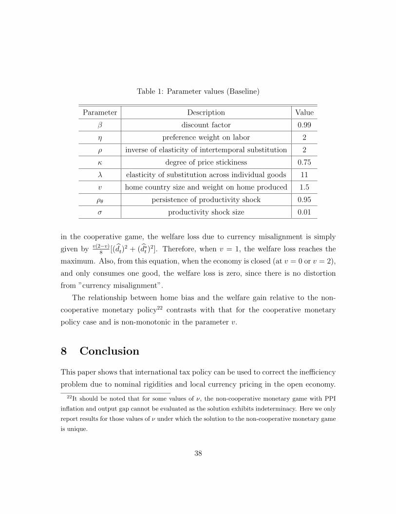
Table 1: Parameter values (Baseline)

Parameter Description Value

β discount factor 0.99

η preference weight on labor 2

ρ inverse of elasticity of intertemporal substitution 2

κ degree of price stickiness 0.75

λ elasticity of substitution across individual goods 11

v home country size and weight on home produced 1.5

ρθ persistence of productivity shock 0.95

σ productivity shock size 0.01

in the cooperative game, the welfare loss due to currency misalignment is simply

given by v(2−v)8

[(dt)2 + (d∗t )

2]. Therefore, when v = 1, the welfare loss reaches the

maximum. Also, from this equation, when the economy is closed (at v = 0 or v = 2),

and only consumes one good, the welfare loss is zero, since there is no distortion

from ”currency misalignment”.

The relationship between home bias and the welfare gain relative to the non-

cooperative monetary policy22 contrasts with that for the cooperative monetary

policy case and is non-monotonic in the parameter v.

8 Conclusion

This paper shows that international tax policy can be used to correct the inefficiency

problem due to nominal rigidities and local currency pricing in the open economy.

22It should be noted that for some values of ν, the non-cooperative monetary game with PPI

inflation and output gap cannot be evaluated as the solution exhibits indeterminacy. Here we only

report results for those values of ν under which the solution to the non-cooperative monetary game

is unique.

38

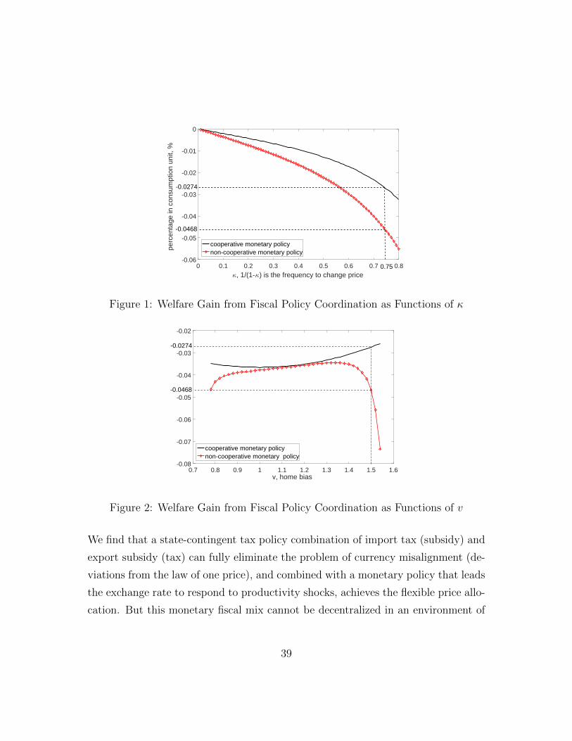
0 0.1 0.2 0.3 0.4 0.5 0.6 0.7 0.8, 1/(1- ) is the frequency to change price

-0.06

-0.05

-0.04

-0.03

-0.02

-0.01

0

perc

enta

ge in

con

sum

ptio

n un

it, %

cooperative monetary policynon-cooperative monetary policy

-0.0274

-0.0468

0.75

Figure 1: Welfare Gain from Fiscal Policy Coordination as Functions of κ

0.7 0.8 0.9 1 1.1 1.2 1.3 1.4 1.5 1.6v, home bias

-0.08

-0.07

-0.06

-0.05

-0.04

-0.03

-0.02

cooperative monetary policynon-cooperative monetary policy

-0.0274

-0.0468

Figure 2: Welfare Gain from Fiscal Policy Coordination as Functions of v

We find that a state-contingent tax policy combination of import tax (subsidy) and

export subsidy (tax) can fully eliminate the problem of currency misalignment (de-

viations from the law of one price), and combined with a monetary policy that leads

the exchange rate to respond to productivity shocks, achieves the flexible price allo-

cation. But this monetary fiscal mix cannot be decentralized in an environment of

39

fully ‘self-reliant’ monetary and fiscal policy. The reason is that the non-cooperative

use of taxes and subsidies to offset the inefficiencies of currency misalignment opens

up a strategic inefficiency in a non-cooperative setting which leads to a fundamen-

tal conflict between the goals of output gap and inflation stabilization and terms

of trade manipulation. The implementation of an efficient monetary-fiscal mix re-

quires effective coordination in fiscal policy, while leaving monetary policy to be

determined non-cooperatively.

40

References

[1] Adao, B., I. Correia, and P. Teles [2009], ”On the relevance of exchange rate regimes

for stabilization policy,” Journal of Economic Theory, 144(4), 1468–1488.

[2] Barbiero, Omar, Emmanuel Farhi, Gita Gopinath, and Oleg Itskhoki [2017]. ”The

Economics of Border Adjustment Tax,” working paper.

[3] Beetsma, Roel M.W.J. and Henrik Jensen [2005]. “Monetary and Fiscal Policy In-

teractions in a Micro-founded Model of a Monetary Union,” Journal of International

Economics, 67(2), 320-352.

[4] Benigno, Gianluca and Bianca De Paoli. 2010. ”On the International Dimension of

Fiscal Policy.” Journal of Money, Credit and Banking, 42(8), 1523-1542.

[5] Benigno, Gianluca and Pierpaolo Benigno, [2006]. “Designing Targeting Rules for

International Monetary Policy Cooperation,” Journal of Monetary Economics, 53(3),

473-506.

[6] Benigno, Pierpaolo and Michael Woodford [2003]. “Optimal Monetary and Fiscal

Policy: A Linear-Quadratic Approach,” NBER Macroeconomics Annual 2003, 18,

271-333.

[7] Benigno, Pierpaolo and Michael Woodford [2005]. “Inflation stabilization and welfare:

The case of a distorted steady state,” Journal of the European Economic Association,

3(6), 1185-1236.

[8] Clarida, Richard, Jordi Galı and Mark Gertler [2002]. “A Simple Framework for

International Monetary Policy analysis,” Journal of Monetary Economics, 49(5), 879-

904.

[9] Correia, Isabel, Juan Pablo Nicolini, and Pedro Teles [2008]. ”Optimal Fiscal and

Monetary Policy: Equivalence Results,” Journal of Political Economy, 116(1), 141-

170.

41

[10] Corsetti, Giancarlo, and Paolo Pesenti [2001]. “Welfare and Macroeconomic Interde-

pendence,” The Quarterly Journal of Economics, 116(2), 421-445.

[11] Corsetti, Giancarlo, and Paolo Pesenti [2002]. “Self-Validating Optimal Monetary

Currency Areas,” NBER Working Paper, No. 8783.

[12] Devereux, Michael B., and Charles Engel [2003], ”Monetary Policy in the Open Econ-

omy Revisited: Price Setting and Exchange Rate Flexibility,” Review of Economic

Studies, 70(4), 765-783.

[13] Devereux, Michael B., Charles Engel, and Peter Storgaard [2004], ”Endogenous Ex-

change Rate Pass-through When Nominal Price are Set in Advance,” Journal of

International Economics 63(2), 263-291.

[14] Devereux, Michael B., Kang Shi and Juanyi Xu [2005], ”Friedman Redux : Restrict-

ing Monetary Policy Rules to Support Flexible Exchange Rates,” Economics Letters

87(3), 291-299.

[15] Devereux, Michael B., Kang Shi and Juanyi Xu [2007], ”The Global Monetary Policy

under a Dollar Standard,” Journal of International Economics, 71(1), 113-132.

[16] Dixit, Avinash and Luisa Lambertini [2003]. “Symbiosis of Monetary and Fiscal

policies in a Monetary Union,” Journal of International Economics, 60(2), 235-247.

[17] Engel Charles [2011], ”Currency Misalignments and Optimal Monetary Policy: A

Reexamination”, The American Economic Review, 101(6), 2796-2822

[18] Farhi, Emmanuel, Gita Gopinath, and Oleg Itskhoki [2013], ”Fiscal Devaluations”,

Review of Economic Studies, 81(2), 725-760.

[19] Fujiwara Ippei and Jiao Wang [2017], ”Optimal Monetary Policy in Open Economies

Revisited”, Journal of International Economics, 108, 300-314.

42

[20] Gali, Jordi and Tommaso Monacelli [2008]. “Optimal Monetary and Fiscal Policy in

a Currency Union,” Journal of International Economics, 76(1), 116-132.

[21] Hevia, Constantino and Juan Pablo Nicolini. [2013]. “Optimal devaluations,” Mimeo,

Department of Economics, UC Berkeley. IMF Economic Review, 61(1), 22-51

[22] Mundell, Robert A.[1961]. ” A Theory of Optimum Currency Areas,” The American

Economic Review, 51(4), 657-665.

[23] Obstfeld, Maurice, and Kenneth Rogoff [1998], ”Risk and Exchange Rates,” NBER

Working Papers 6694.

[24] Obstfeld, Maurice, and Kenneth Rogoff [2000], ”New Direction for Stochastic Open

economy Models,” Journal of International Economics, 50(1), 117-157.

[25] Obstfeld, Maurice, and Kenneth Rogoff [2002], ”Global Implication of Self-Orientnted

National Monetary Rules,” Quarterly Journal of Economics, 117(2), 503-535.

[26] Schmitt-Grohe, Stephanie and Martin Uribe [2005]. “Optimal Fiscal and Monetary

Policy under Sticky Prices,” Journal of Economic Theory, 114(2), 198-230.

[27] Schmitt-Grohe, Stephanie and Martin Uribe [2011], ”Pegs and Pain,” Columbia Uni-

veristy

[28] Senay, Ozge and Alan Sutherland. [2007]. “ Optimal Monetary Policy and the Timing

of Asset Trade in Open Economies.” Economics Letters 95 (2): 297-302.

[29] Senay, Ozge and Alan Sutherland. [2013]. “ The Timing of Asset Trade and Optimal

Policy in Dynamic Open Economies.” Macroeconomic Dynamics 17 (8): 1543-1573.

[30] Siu, Henry [2004] “Optimal Fiscal and Monetary Policy with Sticky Prices,” Journal

of Monetary Economics, 51, 575-607.

[31] Shi, Kang and Juanyi Xu [2007]. “Optimal Monetary Policy with Vertical Production

and Trade,” Review of International Economics, 15 (3), 514-537.

43

[32] Tille, Cedric [2002]. “ How Valuable is Exchange Rate Flexibility? Optimal Monetary

Policy Under Sectoral Shocks?” Federal Reserve Bank of New York Staff Report 147.

44