EXCHANGE RATE REGIMES AND FISCAL PERFORMANCE.

DO FIXED EXCHANGE RATE REGIMES GENERATE MORE

DISCIPLINE THAN FLEXIBLE ONES?

Guillermo Javier Vuletin* University of Maryland

March 2003

Abstract This paper analyzes the influence of exchange rate regimes on fiscal performance, focusing on the difference between fixed and flexible exchange rates. For these ends, a sample of 83 countries for the 1974-1998 period, the GMM methodology for dynamic proposal panel models proposed by Arellano and Bond (1991) and diverse exchange rate classifications are used. In relation to the latter, this paper discusses recent regime classifications and proposes a new exchange rate classification that permits to cover possible inconsistencies between the commitment of the central bank and its observed behavior. The results suggest that the influence of regimes on fiscal performance depend on the international context, specifically the possibility of indebtedness and of the characteristics of the international finance system –integration, volatility and dominant financial structure-. In other words, it depends on credit availability as well as on the conditions or potential sanctioning of the finance system. It is found that in situations in which there is no original fiscal discipline and the authorities have the possibility of financing with debt of relatively low cost, fixed regimes do not purvey per se greater fiscal discipline than the flexible ones. On the contrary, flexible ones generate more discipline. In contexts with strong financing restrictions, the discipline’s effects of both regimes are not substantially different. While in situations with abundance of capitals but where they are highly integrated, they are volatile and possibly subject to contagion effect. The same functioning of the international finance system can, through their potential sanction, achieve greater discipline in economies with fixed regimes that wish to stay as such.

Keywords: exchange rate regimes; expenditure; revenues; deficits; international finance system; panel data; internal instruments; GMM.

JEL Classification: C23, H6, F3, E52, F41.

Author ‘s e-mail address: vuletin@econ.bsos.umd.edu

* Modified version of the Master in Economics thesis. Department of Economics. National University of La Plata (UNLP). Director of thesis: Dr. Jorge E. Carrera. December 2001.

I am grateful to Ricardo N. Bebczuc, María L. Garegnani, Leonardo C. Gasparini, Emilio Espino and the participants of the “Seminario de Economia” of the UNLP for their valuable commentaries and sugestions and especially to Walter E. Sosa Escudero for his generous disposition to clarify econometric matters. Any mistakes or omisions are of my responsability.

Another version of this paper participated in a contest for the “Professor Elias Salama” award during the Seventh Meeting of Monetary and International Economy (2002), organized by the Economics Department of the UNLP, in which it was awarded with the first prize.

2

CONTENTS

1 INTRODUCTION 3

2 THEORETICAL DISCUSSION 4

3 ECONOMETRIC METHODOLOGY 8

4 DATA 10

4.1 MACROECONOMIC AND FISCAL VARIABLES 10 4.2 EXCHANGE RATE REGIMES CLASSIFICATIONS 10

5 EMPIRICAL RESULTS 14

5.1 IMPORTANCE IN THE CHOICE OF THE ESTIMATION METHOD 14 5.2 CONTROLLING ENDOGENEITY FOR VARIABLES THAT INFLUENCE ON THE REGIME CHOICE BUT

NOT ON THE FISCAL PERFORMANCE 15 5.3 THE ROLE OF INTERNATIONAL MARKETS 15 5.4 LONG AND SHORT TERM FIXED REGIMES: SHORT PEG AND LONG PEG 19 5.5 NEW EXCHANGE CLASSIFICATION: THE IMPORTANCE OF A CLASSIFICATION DETECTING

INCONSISTENCIES 20

6 CONCLUSIONS 23

7 REFERENCES 25

8 DATA APPENDIX 28

8.1 COUNTRIES’ SAMPLES 28 8.2 MACROECONOMIC VARIABLES’ DEFINITIONS 28

9 TABLES APPENDIX 30

3

1 INTRODUCTION

Before the fall of the Bretton Woods system in 1973, most of the countries had fixed exchange

regimes. Since then, countries have experienced with varied exchange rate regimes. The

evaluation of the costs and benefits associated with the different regimes has been the source

of many debates and continuous to be one of the most important in international economy in

our days. In theoretical terms, it is difficult to establish a univocal consensus on this relation

product of the many links –that are partly reinforced and partly counteracted– among the

different exchange rate regimes and the macroeconomic variables. Precisely, the relevance of

the empirical analysis consists of trying to quantify the relative importance of the different

relations involved.

There are many empirical studies that analyze the impact of exchange rate regimes on

different macroeconomic variables such as inflation and its volatility, money growth, real

interest rate, product growth and its volatility. An issue that has not been deeply analyzed is

the relation between exchange rate regimes and fiscal performance. The aim of this paper is to

set out the relative importance of these links, specifically analyzing the regime influence on

fiscal behavior.

Apart from informal discussions, the few existing empirical studies can be divided in two

groups according to the type of analysis. On the one hand, the first group comprises papers

like those of Tornell and Velasco (1995b) and Alfaro (1999), which recur to the analysis of

episodes for certain countries –generally from Latin America-. Even if these can provide

evidence in favor or against some hypotheses, it is not possible to isolate the effects of the

different variables involved. On the other hand, the second group is formed by research such

as that of Tornell and Velasco (1995a), Bazzoni and Nashashibi (1994) and Adam et al. (2000),

who limit the analysis to the Sub-Sahara region in Africa to eliminate potential endogeneity

problems in regime choice. This is because the countries that belong to the Franc Zone

maintained a fixed regime from 1948 to 1994 and because this choice was due to political

issues associated to colonial history and not to economic motives.

This paper surpasses previous analysis limitations covering a maximum sample of 83

countries during the 1974-1998 period. At the same time that it finds evidence on the

influence of exchange rate regimes on fiscal performance, it provides a possible criterion for

regime election.

The empirical analysis expands and improves previous literature in many regards:

• It allows, unlike episode analysis, to work out the effect of exchange rate regimes on fiscal

performance considering other variables that can affect this performance.

4

• It advances towards the use of a dynamic methodology of estimation (Generalized

Method of Moments), which considers endogeneity problems and unobserved specific effects,

which generate bias in estimations performed by fixed effects if the dependant variable has a

strong persistence or temporal inertia.

• The correction of potential endogeneity problems, together with the inclusion of variables

that affect regime election, makes it possible to incorporate economies of different regions.

• It makes an extensive use of available information on the classification of exchange rate

regimes, widening the dichotomy "fixed vs. flexible” according to de jure classification

compiled by IMF, and of new contributions by Levy Yeyati and Sturzenegger (2000) in

relation to the classification according to behavior. In this sense, a new classification of

exchange rate regimes is realized, making it possible to cover probable inconsistencies

between the commitment of the Central Bank -of intervening and subordinating its monetary

policy to the currency market- and its behavior.

• It evaluates fiscal performance in many ways -total deficit, primary deficit, total

expenditure, primary expenditure and revenues-, trying to capture not only the effect of the

regime on an aggregated variable –defined on the basis of other variables- such as deficit, but

also on “original” variables allowing to distinguish potential transmission mechanisms. Also,

total and primary concepts of fiscal variables are used, making it possible to indirectly

observe the links between the variables and the debt interests.

• Diverse sub-periods that characterize the level of capital market integration, indebtedness

possibility and the dominant finance structure are considered, analyzing if these

characteristics modify the influence of the regime on fiscal performance.

The paper is organized as follows: section 2 does a revision on the most representative

theoretical and empirical works; section 3 justifies econometric methodology choice; section 4

presents the macroeconomic variables and diverse exchange classifications that are used;

section 5 shows the econometric results; section 6 presents the conclusions.

2 THEORETICAL DISCUSSION

Traditionally, the explanations about exchange rate policies were based on the theory of

optimal areas of Mundell (1960 and 1961), determining how different exchange rate regimes

could be desirable for countries with different characteristics. For example, small and open

countries having economies that are not very subjected to price shocks should have a more

fixed regime. Even though the traditional approximation was extremely useful in the past, it

does not prove to be that useful nowadays given that it considers the choice of regime as if it

5

were made in vacuo, where each regime can be instantaneously placed and indefinitely

sustained. As history shows, exchange rate regimes are not chosen once and forever but are

frequently changed, either voluntarily or involuntarily.

More recently, attention has been centered in the potential credibility effects of the exchange

rate policy, emerging a trade-off between credibility and flexibility. The theoretical studies

that analyze the relation between regimes and fiscal performance cover mainly four fields of

study of Economics: dynamic stochastic models, the so-called stabilization policies, issues

linked to political economy and studies that relate the recent crisis of the nineties with

growing integration and volatility of the capitals market.

The first group consists of those papers based on dynamic stochastic models of general

equilibrium, which analyze the results of technological, monetary and government

expenditure shocks under different exchange rate regimes. Some of them are: Obstfeld and

Rogoff (1995b and 1998), Bachetta and van Wincoop (1999) and Devereux (1999). The latter

outlines that the effect of the exchange rate regime on macroeconomic variables depends on

the regime as well as on the monetary policy that is being implemented.

The second group, which is related to stabilization policies, includes many papers among

which are those by Aghevli et al. (1991), Frenkel et al. (1991), Giavazzi and Pagano (1988), and

Weber (1991). Their conventional vision supports the idea that fixed regimes provide more

fiscal discipline than the flexible ones due to the adoption of lax fiscal policies, would lead to

an exhaustion of reserves and consequently to the collapse of the peg. As presumably, the

eventual collapse of the fixed exchange rate would imply a big political cost for the policy

maker, this one would be disciplined, causing unsustainable fiscal policies not to occur in

equilibrium. In other words devaluation is not an option, which is of course an

oversimplification, because as history repeatedly shows, fixed regimes usually fail to impose

discipline and generally end in devaluation crises1.

In relation to a most recent branch linked to issues of political economy, Tornell and Velasco

(1994, 1995a and 1995b), Alfaro (1999), Velasco (1997), and Alberola and Molina (2000) can be

named. Tornell and Velasco (1994, 1995a and 1995b) support that there are empirical and

theoretical problems with the kind of lines of thought exposed by conventional papers on

policy stabilization. They consider a fiscal authority prone to spend more than what is socially

desirable and with a lower discount rate after a certain moment –for example, because of

uncertainty about re-election- and, a central bank that can precommit not to finance the

1 See for example Calvo and Vegh (1996), Cooper (1971) and Kamin (1988).

6

deficits incurred by the fiscal authority for a finite period of time. They conclude that the

difference in fiscal behavior among regimes lies in the intertemporal distribution of the costs.

Under fixed regimes, unsound policies are manifested in falling reserves or exploding debts,

making their costs effective only when the situation is unsustainable. While with flexible

regimes, they are immediately manifested through movements in the exchange rate and the

price level. Therefore, being inflation costly for the fiscal authority, flexible regimes can

provide more fiscal discipline. It is important to outline that the previous result depends, on

one hand, on the possibility of intertemporal choice for the policymaker, because if it does not

have access to credit and/or if it had insufficient reserves, money-financed deficits would

inevitably cause an immediate depreciation, regardless of the exchange rate regime. On the

other hand, it is essential that the central bank can precommit not to accommodate the wishes

of the fiscal authority only for a finite period of time because, if this commitment were

forever, the equivalence between regimes found by Helpman (1981) would persist.

Velasco (1997) develops a model analogous with that discussed in Alesina and Drazen (1991)

in which he rationalizes debt bubbles and post-stabilization programs. That is, it gives

rationality to the phrase “things must be really bad before they start to get better again”. So,

he recurs to a model with interest groups where the resources of the government are seen as

common property. On the one hand, he finds that deficits can be held through fiscal reform,

but that will only happen after a long and intense period of government indebtedness and, on

the other hand, that the deficit bias will be greater as greater is the fragmentation level of the

interest groups.

From a distributive point of view, Alfaro (1999) justifies why governments hold policies that

are presumed not to be sustainable in the long run. Considering heterogeneity in the

population as regards its dotations, whether they have transable or non-transable goods, it

argues that the real exchange rate appreciation associated to stabilization plans improves the

position of the latter.

Since the exchange rate and finance crises of the nineties, there has been a great upsurge of

literature that analyzes the role of growing integration and volatility of capital markets upon these

crises. Some of these papers are by Chang and Velasco (1998), Meng and Velasco (1999),

Chang (1999), and Velasco (1996). In general, they analyze credibility policy problems and

finance structure problems combined with herd behavior, contagion effect and financial

frictions as main elements in recent crises. Chang (1999) divides the recent disscusions that try

to explain the crises in growing capital markets into two groups. On the one hand, he

considers those under the “bad policy view” that, in agreement with the spirit of Krugman’s

first generation crises (1979), suggest that crises are the inevitable result of inconsistent

7

policies. On the other hand, he considers those under the “financial panic view”, who

maintain that fundamentals do not seem to be good predictors and that, on the contrary, the

expectations of the market subject to herd behaviors and contagion effect are the key to

understand the nineties’crises.

Chang and Velasco (1998) analyze interaction between banking fragility and exchange rate

regimes, basing themselves on microfundamentals of the financial system, taking as

benchmark Diamond and Dybvig’s model (1983). They find that this fragility is evident in

fixed regimes. A drastic change in public trust can cause a fall in banking deposits and,

possibly, a run on deposits. Under fixed regimes, the central bank has the following trade-off.

If nothing were done, a wave of banking bankruptcy would occur and consequently a serious

interruption of the economic activity. If it purveyed credits to the most affected banks, these

credits would rapidly return to the central bank in the form of a greater demand of

international reserves, causing the collapse of fixed exchange rate. On the contrary, with

flexible regimes and a central bank acting as lender of last resort, banking runs on deposits

originated by unfulfilled expectations can be eliminated.

Velasco (1996) extends the Barro-Gordon model to a dynamic context in which the level of the

state variable, in this case the debt stock, determines the sustainability of the fixed exchange

rate. Considering that reputation matters and that there is a fixed cost for devaluation, he

finds that fixed regime is sustainable if and only if the debt stock is sufficiently low. There is a

debt rank in which multiple equilibriums are obtained, where the devaluation result depends

on the expectations of the agents. While for a certain level of high debt, there is an

equilibrium where the speculative attack occurs with positive probability, promoting the

decrease in debt size on the side of the government. That is, for the fixed exchange rates to be

really fixed, the debt must be smaller if investors are voluble -in the sense of being prone to

panic-.

The study of all this literature suggests many questions: Do fixed regimes provide more fiscal

discipline than flexible ones? Does the possibility of government indebtedness modify the

effect of exchange rate regimes on fiscal performance? Do greater integration and volatility of

the current international financial system have any special effect on fiscal behavior in

economies with fixed exchange rate regimes? Did stabilization programs of the eighties

promote greater fiscal discipline? The aim of this paper is to respond to these questions and

others that may arise as this analysis goes further.

8

3 ECONOMETRIC METHODOLOGY

For the selection of the estimation method three aspects were considered. In the first place,

issues concerning data. Due to the availability of panel data -which make it possible to retain

all the information in relation to the use of annual averages - the presence of the country’s

unobservable factors must be enabled. Secondly, particularities of the dependent variable

must be considered. Fiscal performance in its diverse forms of measurement has a dynamic

nature –as table 9-1 shows-, reason for which the methodology must allow for an inertia

behavior of this variable. A third element is the so-called “reverse causality”. That is, as some

of the explanatory variables are likely to be jointly determined with fiscal behavior,

endogeneity of the explanatory variables must be controlled.

Considering these aspects, the appropriate methodology to use is the Generalized-Method-of-

Moments (GMM) estimator for dynamic panel data models developed by Arellano and Bond

(1991). This estimator deals with country specific effects and potential endogeneity of the

explanatory variables. The control for endogeneity is achieved by using “internal

instruments” (i.e., instruments based on lagged values of the explanatory variables).

What follows is a brief presentation and justification of the chosen methodology and its

benefits as regards the frequently used alternatives. The dynamic nature of the fiscal

performance (F) must be represented through a model containing lagged dependent variables

among the regressors. To simplify the analysis, a simple autoregressive model with one lag

period of the dependent variable is considered:

itittiit xFF υβδ ++= −'

1, Ni ,...,1= Tt ,...,1= (1)

Where δ is a scalar, 'itx of dimension 1xk represents a group of variables that potentially

affect fiscal performance, and β is of kx1. Assuming that the itυ follow a one-way error

component model:

itiit νµυ += (2)

Where iµ ~ IID ),0( 2µσ and itν ~ IID ),0( 2

νσ are independent of each other and among

themselves.

In these dynamic models, the implications of the election of diverse estimation techniques

have a different nature from those associated to static models. Since itF is a function of iµ ,

1, −tiF is also a function of iµ . Therefore, 1, −tiF , a right-hand regressor in (1), is correlated

with the error term. This renders the Ordinary Least Square (OLS) estimator biased and

inconsistent even if the itν are not serially correlated. In relation to the Fixed Effect (FE)

9

estimator, the Within transformation wipes out the iµ , though ( 1,1, −− − titi FF ) where

∑=

−− −=T

ttiti TFF

21,1, )1( will still be correlated with )( iit νν − even if the itν are not

serially correlated. This is because 1, −tiF is correlated with iν by construction. The latter

average contains 1, −tiν which is obviously correlated with 1, −tiF . In fact, the Within

estimator will be biased and only if ∞→T will the Within estimator of δ and β be

consistent for the dynamic error component model. The same problem springs with the

random effects Generalized Least Square estimator (GLS) because )( 1,1, −− − titi FF θ will

be correlated with )( 1,, −− titi υθυ .

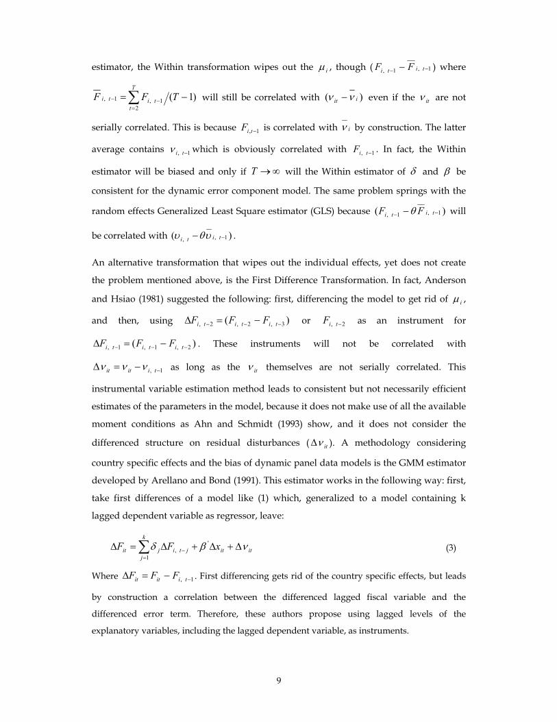
An alternative transformation that wipes out the individual effects, yet does not create

the problem mentioned above, is the First Difference Transformation. In fact, Anderson

and Hsiao (1981) suggested the following: first, differencing the model to get rid of iµ ,

and then, using )( 3,2,2, −−− −=∆ tititi FFF or 2, −tiF as an instrument for

)( 2,1,1, −−− −=∆ tititi FFF . These instruments will not be correlated with

1, −−=∆ tiitit ννν as long as the itν themselves are not serially correlated. This

instrumental variable estimation method leads to consistent but not necessarily efficient

estimates of the parameters in the model, because it does not make use of all the available

moment conditions as Ahn and Schmidt (1993) show, and it does not consider the

differenced structure on residual disturbances ( itν∆ ). A methodology considering

country specific effects and the bias of dynamic panel data models is the GMM estimator

developed by Arellano and Bond (1991). This estimator works in the following way: first,

take first differences of a model like (1) which, generalized to a model containing k

lagged dependent variable as regressor, leave:

itit

k

jjtijit xFF νβδ ∆+∆+∆=∆ ∑

=−

'

1, (3)

Where 1, −−=∆ tiitit FFF . First differencing gets rid of the country specific effects, but leads

by construction a correlation between the differenced lagged fiscal variable and the

differenced error term. Therefore, these authors propose using lagged levels of the

explanatory variables, including the lagged dependent variable, as instruments.

10

The GMM estimator will be consistent if the lagged levels of explanatory variables are valid

instruments for differenced explanatory variables. This will hold if the error term is not

serially correlated. These assumptions can be tested through the tests proposed by Arellano

and Bond (1991). The first is a Sargan test of overidentifying restrictions, which tests the

overall validity of the instruments. Failure to reject the null hypothesis gives support to the

model. The second is a test for serial correlation in the error term. If such test does not reject

the null hypothesis of second order correlation absence, it can be concluded that the original

error term does not have serial correlation.

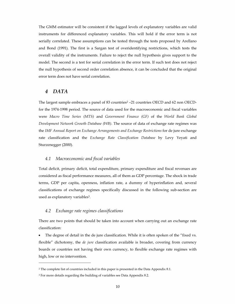
4 DATA

The largest sample embraces a panel of 83 countries2 –21 countries OECD and 62 non OECD-

for the 1974-1998 period. The source of data used for the macroeconomic and fiscal variables

were Macro Time Series (MTS) and Government Finance (GF) of the World Bank Global

Development Network Growth Database (WB). The source of data of exchange rate regimes was

the IMF Annual Report on Exchange Arrangements and Exchange Restrictions for de jure exchange

rate classification and the Exchange Rate Classification Database by Levy Yeyati and

Sturzenegger (2000).

4.1 Macroeconomic and fiscal variables

Total deficit, primary deficit, total expenditure, primary expenditure and fiscal revenues are

considered as fiscal performance measures, all of them as GDP percentage. The shock in trade

terms, GDP per capita, openness, inflation rate, a dummy of hyperinflation and, several

classifications of exchange regimes specifically discussed in the following sub-section are

used as explanatory variables3.

4.2 Exchange rate regimes classifications

There are two points that should be taken into account when carrying out an exchange rate

classification:

• The degree of detail in the de jure classification. While it is often spoken of the “fixed vs.

flexible” dichotomy, the de jure classification available is broader, covering from currency

boards or countries not having their own currency, to flexible exchange rate regimes with

high, low or no intervention. 2 The complete list of countries included in this paper is presented in the Data Appendix 8.1.

3 For more details regarding the building of variables see Data Appendix 8.2.

11

• The criterion to follow when carrying out the classification. Economic literature shows

two possible options to carry it out: a de jure classification, based on the commitment adopted

by the central banks; and a de facto classification, product of the actual behavior. Neither of the

methods is entirely satisfactory. The de facto classification has the advantage that it is based on

the observed behavior, but does not make it possible to distinguish between stable nominal

exchange rates resulting from the absence of shocks, and the stability produced by political

actions counteracting the shocks. Because of this, it fails to capture what might be the essence

of an exchange rate regime -the type of commitment of the central bank to intervene and

subordinate its money policies to the currency market. The de jure classification captures this

formal commitment, but fails to control policies, which are inconsistent with this

commitment.

Taking these two points into consideration, three exchange classifications are used:

• Initially, a three-category de jure classification is considered: fixed, intermediate and flexible.

The fixed regimes cover: a single currency peg; SDR peg; other official basket pegs; and a

secret basket peg, according to the IMF terminology. The intermediate group includes:

cooperative arrangement, unclassified flexible, rule based, crawling peg and target zone.

While the flexible group includes independent float and managed floating.

There were two questions in this way of grouping:

The first was associated to the managed float category. It was decided to consider it as

floating because for the topics and variables involved it is more relevant to know whether

there is a commitment on the part of the central bank or not than if they effectively intervene

or not in the currency market. In fact, according to Levy Yeyati and Sturzenegger (2000), only

a bit more than 30% of the countries said to have a floating exchange rate regime, behave as

such.

The second question is how to classify the countries participating in the European “snake” in

the mid seventies and later in the EMS. These countries have fixed exchange rate regimes, but

they float against other currencies. In agreement with other papers -Ghosh et al. (1997) and

Levy Yeyati and Sturzenegger (2000)-, it is classified as intermediate.

• The second exchange classification differentiates long or short term de jure fixed regimes,

depending on whether they have been defined as such, at least five consecutive years, or not

respectively. This leads to a four-category classification: longpeg, shortpeg, intermediate and

flexible.

• The third exchange rate classification is the one suggested by this paper, which captures

both the central bank commitment to intervene and subordinate its monetary policy to the

12

currency market, and the likely inconsistencies in its behavior. For this, de jure classification

of the IMF and de facto classification by Levy Yeyati and Sturzenegger (2000)4 are combined

under a grouping criterion.

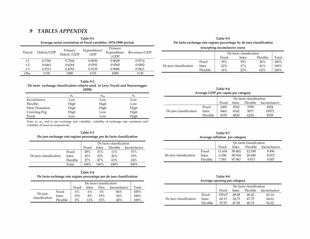
Tables 9-3 up to 9-5 describe, through the “crossing” of de jure and de facto classifications, the

main characteristics of the regimes for the 1974-1998 period in quantitative terms, while tables

9-6 up to 9-8 do the same following some of the macroeconomic variables used in the

analysis. Some of the most outstanding characteristics are:

- An important proportion of the de facto inconclusive regimes are present for all the de jure

exchange rate regimes, especially for fixed regimes (table 9-4). At the same time the greatest

proportion of inconclusive regimes are concentrated in de jure fixed regimes (table 9-3).

- While 63% of the regimes showing a flexible behavior are defined as such, just 28% of the

ones behaving as fixed admit being so (table 9-3). This behavior –paraphrasing Calvo and

Reinhart (2000)- could be refer to as “fear of pegging”. And could result from a desire of

reduction of exposure to speculative attacks associated to explicit compromises.

- Excluding the inconclusive ones, while 62% of de jure flexible regimes behave as such, just

39% of the fixed ones does so (table 9-5). This result shows an important difference between

the central bank commitment to intervene and the behavior observed according to the

exchange rate regimes.

- The economies with de jure fixed regimes are open economies with low GDP per capita,

especially for those which are also de facto fixed (tables 9-6 and 9-8).

- As regards the inflationary performance, the de facto intermediate regimes show the highest

rates for each de jure regime; and de facto fixed regimes have lower average rate than the

flexible ones (table 9-7).

On the basis of the characteristics mentioned above, the theoretical and empirical elements

considered for building the new classification of exchange rate regimes are:

- The categories’ diversity should balance a trade-off between greater information and

restrictions imposed by econometric issues.

- A clear difference between commitment and behavior, according to de jure exchange rate

regimes, is observed, with greater divergence for fixed regimes.

- The categories’ diversity should consider the performance or explanatory capacity of the

different possible categories. For example, while it seems to be obvious that a country with

4 Specifically the 1st round classification is considered, as it emerges from a deeper analysis likely to eliminate the possible bias towards the irrelevance of the significance of the regime. The outline of the criterion considered by Levy Yeyati and Sturzenegger (2000) is presented in table 9-2.

In this paper the dirty floating categories and crawling peg by Levy Yeyati and Sturzenegger (2000) were grouped under de facto intermediate category.

13

a de jure fixed regime showing an intermediate or flexible behavior is inconsistent with this

commitment, it is not clear that an economy with flexible regime, behaving as fixed, violates

any kind of commitment which makes it inconsistent.

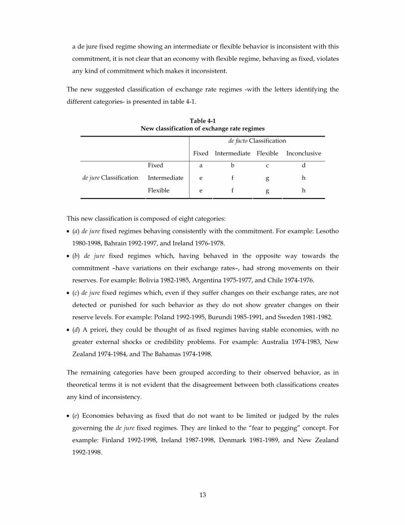
The new suggested classification of exchange rate regimes -with the letters identifying the

different categories- is presented in table 4-1.

Table 4-1 New classification of exchange rate regimes

de facto Classification

Fixed Intermediate Flexible Inconclusive

Fixed a b c d

Intermediate e f g h de jure Classification

Flexible e f g h

This new classification is composed of eight categories:

• (a) de jure fixed regimes behaving consistently with the commitment. For example: Lesotho

1980-1998, Bahrain 1992-1997, and Ireland 1976-1978.

• (b) de jure fixed regimes which, having behaved in the opposite way towards the

commitment –have variations on their exchange rates–, had strong movements on their

reserves. For example: Bolivia 1982-1985, Argentina 1975-1977, and Chile 1974-1976.

• (c) de jure fixed regimes which, even if they suffer changes on their exchange rates, are not

detected or punished for such behavior as they do not show greater changes on their

reserve levels. For example: Poland 1992-1995, Burundi 1985-1991, and Sweden 1981-1982.

• (d) A priori, they could be thought of as fixed regimes having stable economies, with no

greater external shocks or credibility problems. For example: Australia 1974-1983, New

Zealand 1974-1984, and The Bahamas 1974-1998.

The remaining categories have been grouped according to their observed behavior, as in

theoretical terms it is not evident that the disagreement between both classifications creates

any kind of inconsistency.

• (e) Economies behaving as fixed that do not want to be limited or judged by the rules

governing the de jure fixed regimes. They are linked to the “fear to pegging” concept. For

example: Finland 1992-1998, Ireland 1987-1998, Denmark 1981-1989, and New Zealand

1992-1998.

14

• (f) They have important movements in their reserves, and changing and volatile exchange

rates, but are not engaged with the exchange rate fixation. For example: Argentina 1981-

1985, Brazil 1987-1993, and Thailand 1997-1998.

• (g) Within this classification, it is really close to pure flexible as it does have important

variations in the exchange rate but little movement on its reserves. For example: the United

States 1977-1998, Japan 1977-1998, Turkey 1981-1993, Chile 1992-1995, Uruguay 1986-1988 y

1990-1996.

• (h) They include stable economies with no important or strong-enough external shocks as to

avoid greater effects on their exchange rates or reserves. For example: Belgium 1974-1998,

Canada 1974-1997, Tunisia 1987-1998, and Costa Rica 1993-1998.

5 EMPIRICAL RESULTS

In this section, the econometric results are presented. The inclusion of explanatory variables is

not derived from a particular model. On the contrary, it is general enough as to test different

hypotheses. The basic model is assessed for the 1974-1998 period and considers, in addition to

the lagged of the dependent variable, the terms of trade shocks, the GDP per capita, and the

exchange rate regimes as potential determinants of the fiscal variables. Later, the openness

and the inflation are included as control variables. Then, the study advances in two ways: on

the one hand, the model is evaluated at different sub-periods and, on the other hand, the

exchange rate classification is enriched.

It is worth mentioning that the Sargan test and the serial correlation test cannot reject the null

hypothesis for almost all the models estimated through GMM, supporting the use of

appropriate lags of the explanatory variables as instruments for the estimation.

For a proper reading of the coefficients associated with exchange rate regimes, it is worth

reminding that they refer to their differential effect compared to the flexible –de jure flexible in

the IMF classification, and pure flexible for the new classification (category g)-.

5.1 Importance in the choice of the estimation method

Models 1 and 2 of tables 9-9 and 9-13 represent the most basic estimated model. They cover

the 1974-1998 period and consider the current and past values of the shocks in exchange

terms and of the GDP per capita as explanatory variables together with lags of the fiscal

variable and the exchange regimes –fixed, intermediate and flexible. Models 1 and 2 differ in

the estimation methodology depending on whether it is FE or GMM respectively. The results

show the great importance of the proper choice of the method. On the one hand, for all fiscal

variables the estimate by FE increases the importance of the inertial behavior and, on the

15

other hand, the effect of the regimes suffers several changes not only in significance but also

in direction and magnitude.

5.2 Controlling endogeneity for variables that influence on the regime choice but

not on the fiscal performance

Model 2 makes it possible to isolate the effect of each variable, including the regimes, on the

fiscal variable. However, this endogeneity control does not include variables having an

incidence on the regime choice but not a direct influence on the fiscal behavior. In the FE

estimation context this would be solved by the use of simultaneous equations for truncated

endogenous variables as Maddala (1983) suggests. Due to the fact that this proceeding is not

appropriate under GMM estimation, this type of variables were included in the regression

equation as control variables, building model 3, in which openness an inflation are added as

possible determinants of exchange regime, as many papers like Frieden’s et. al. (2000) and

Ghosh’s et. al. (1997) suggest.

Model 3 shows a strong persistence in all fiscal variables, with positive and significant

coefficients. An improvement on the exchange terms increases the total and primary fiscal

balance after many periods because of the increase in fiscal revenues and the decrease in

expenditures, which is consistent with the standard neoclassic approximation through a tax-

smoothing model. However, in the short run the increase in the revenues is compensated by

an increase in the expenditures causing a slight or null improvement in the fiscal balance,

which can be justified with political economy models, in line with the evidence found by

Tornell and Lane (1994) and Talvi and Vegh (2000). As regards the influence of exchange rate

regimes, fixed ones show better fiscal performance over the total expenditure, total deficit and

primary variables. These results would support the conventional view held by Aghevli et al.

(1991), Frenkel et al. (1991), Giavazzi and Pagano (1988), and Weber (1991) according to which

fixed regimes provide greater fiscal discipline.

5.3 The role of international markets

Important issues to be taken into account in order to properly analyze the exchange rate

regime influence on the fiscal performance are indebtedness possibilities and the international

capital market characteristics, especially as regards their level of integration, volatility and

dominant financial structure. As described in the theoretical discussion, indebtedness

possibilities make the possibility of intertemporal choice for the policymaker. Likewise, there

is ample literature that analyzes how some changes in the international financial system

modify its intrinsic functioning:

16

• Dominant financial structure change: while in the seventies and eighties the financial

structure was dominated by banks, since the beginning of the nineties there has existed a

great growth of institutions such as investment, pension and insurance funds which modify

the link and rules between debtors and creditors. As Krueger (2002) explains, while in the

eighties an important proportion of the emerging country debts were in charge of bank

loans and the 85% of the creditors of the debt of a country could be gathered around a table,

in the nineties the bond market has quadruplicated and bond holders are more numerous,

anonymous and hard to coordinate than the banks. This creates a joint action problem, due

to the fact that certain agreements on debt reorganization that had once been achieved are,

in the present context, difficult to achieve.

• New financial instruments’ growth: The previous situations worsen with the growth of debt

instruments and derivates, which allow investors to take short-term positions in weak

currencies through spot, forward and options of the money market. This means that those

countries having fixed regimes, especially those having unsustainable policies and

structural weakness, run the risk of suffering speculative attacks to their currency and of

losing access to the capital market.

• Growing integration: several papers such as Bayoumi (1990) and Jones and Obstfeld (1997)

find a growing integration financial pattern since 1973 through the correlation between

saving and investment.

• Growing volatility of financial flows: Fischer (1999) mentions that even though the nature of

the capital movement is not entirely smooth or predictable, the capital flow volatility in the

nineties seems to be excessive.

• Growing volume of financial flows: the total of financial flows as proportion of the global

product showed a slight growing trend between 1974 and 1982, a decrease in the 1983-1989

period and an important increase in the nineties.

• Contagion effect: Wolf (1997) defines contagion in the financial markets as the co-movement

of markets not ascribable to a common co-movement of the fundamentals. The three ways

that can help to explain this behavior are: the herd behavior –attributed to asymmetric

information problems-, the portfolio’s composition – which makes that any change in the

output of an active in a market contribute to modifications in the rest of the composition-

and the interdependence of the portfolio –which seeks to compensate losses of capital in a

country with the sell of assets from other markets to increase liquidity in view of the rescue

of investors-.

For these reasons, the 1974-1998 period was divided in three sub-periods according to the

capital flow size, the integration level, the volatility and the dominant financial structure:

17

• 1974-1982: This period was characterized for an international financial structure dominated

by bank loans and for an abundance of capitals that allowed strong increases of the debts

that ended with the 1982 crisis.

• 1983-1989: It was a period of strong reduction in the capital flows as a consequence of the

debt crisis originated by Mexico in August 1982, which continued with several crises in

emergent economies such as Argentina, Brazil, Chile and Nigeria.

• 1990-1998: Like in the seventies, it is a period of capital abundance, but unlike the former

the growth of institutions such as investment, pension and insurance funds encouraged a

growing integration of the international financial system that favored the development of

bonds and shares markets. The growing volatility of the financial flows appears as an

outstanding characteristic, which is usually explained by two classes of arguments. On the

one hand, some associate rational motives based on the fundamentals and; on the other

hand, there are arguments -about which most agree- that there are additional irrational

motives, such as the contagion effect or herd behavior, which make the volatility

characteristic of the international investors appear to be boosted by some level of economic

frailty. In this respect, Greenspan (1998) points out: “Recent crises, while sharing many, if

not most, of the characteristics of past episodes, nonetheless, appear different. Market

discipline today is clearly far more draconian and less forgiving than twenty or thirty years

ago. Owing to greater information and more opportunities, capital now shifts more readily

and increasingly to those ventures or economies that appear to excel.”

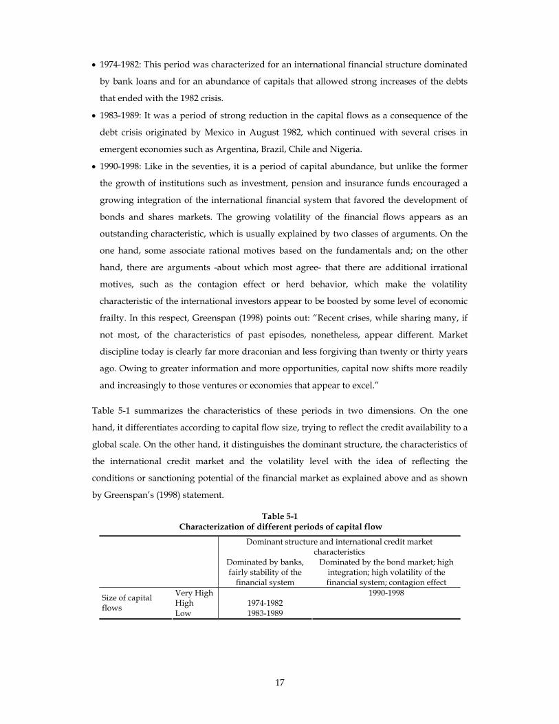
Table 5-1 summarizes the characteristics of these periods in two dimensions. On the one

hand, it differentiates according to capital flow size, trying to reflect the credit availability to a

global scale. On the other hand, it distinguishes the dominant structure, the characteristics of

the international credit market and the volatility level with the idea of reflecting the

conditions or sanctioning potential of the financial market as explained above and as shown

by Greenspan’s (1998) statement.

Table 5-1 Characterization of different periods of capital flow

Dominant structure and international credit market characteristics

Dominated by banks, fairly stability of the

financial system

Dominated by the bond market; high integration; high volatility of the financial system; contagion effect

Very High 1990-1998 High 1974-1982 Size of capital

flows Low 1983-1989

18

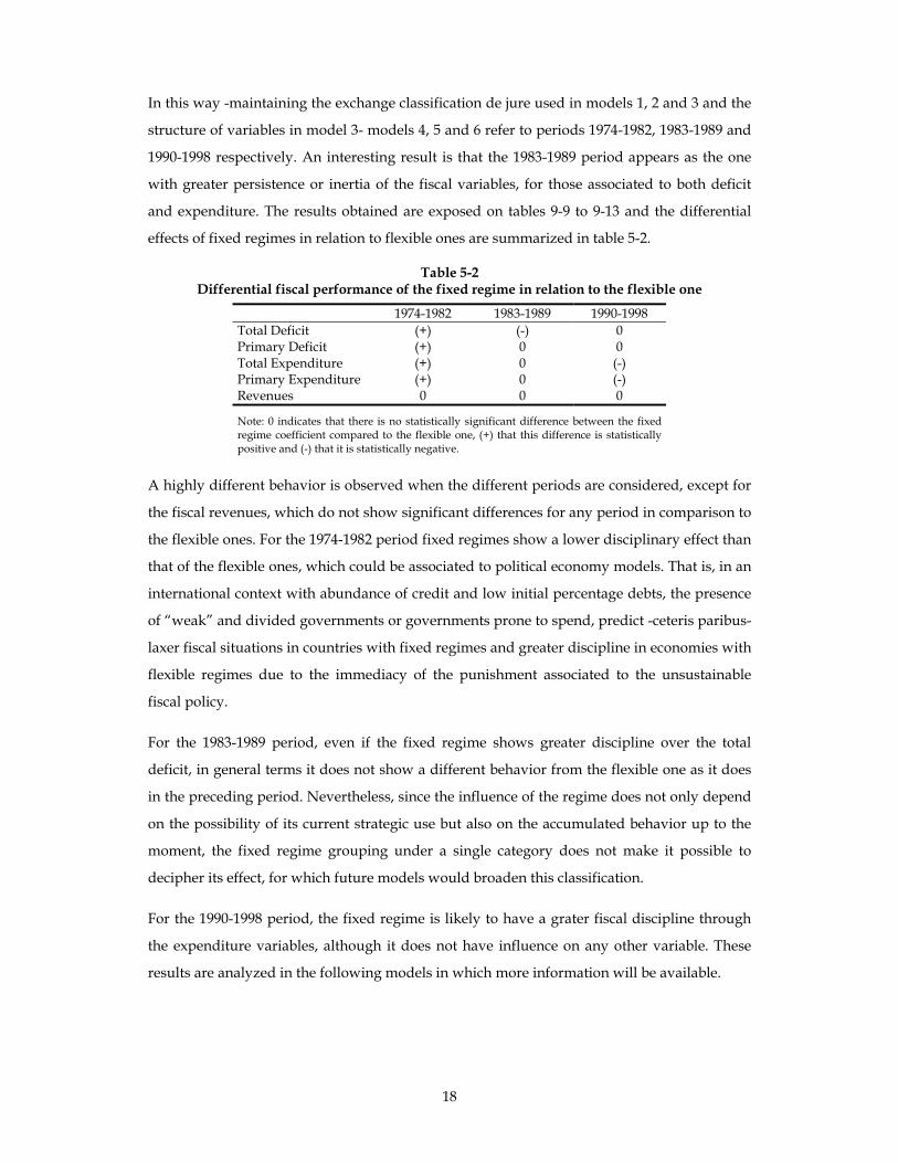
In this way -maintaining the exchange classification de jure used in models 1, 2 and 3 and the

structure of variables in model 3- models 4, 5 and 6 refer to periods 1974-1982, 1983-1989 and

1990-1998 respectively. An interesting result is that the 1983-1989 period appears as the one

with greater persistence or inertia of the fiscal variables, for those associated to both deficit

and expenditure. The results obtained are exposed on tables 9-9 to 9-13 and the differential

effects of fixed regimes in relation to flexible ones are summarized in table 5-2.

Table 5-2 Differential fiscal performance of the fixed regime in relation to the flexible one

1974-1982 1983-1989 1990-1998 Total Deficit (+) (-) 0 Primary Deficit (+) 0 0 Total Expenditure (+) 0 (-) Primary Expenditure (+) 0 (-) Revenues 0 0 0

Note: 0 indicates that there is no statistically significant difference between the fixed regime coefficient compared to the flexible one, (+) that this difference is statistically positive and (-) that it is statistically negative.

A highly different behavior is observed when the different periods are considered, except for

the fiscal revenues, which do not show significant differences for any period in comparison to

the flexible ones. For the 1974-1982 period fixed regimes show a lower disciplinary effect than

that of the flexible ones, which could be associated to political economy models. That is, in an

international context with abundance of credit and low initial percentage debts, the presence

of “weak” and divided governments or governments prone to spend, predict -ceteris paribus-

laxer fiscal situations in countries with fixed regimes and greater discipline in economies with

flexible regimes due to the immediacy of the punishment associated to the unsustainable

fiscal policy.

For the 1983-1989 period, even if the fixed regime shows greater discipline over the total

deficit, in general terms it does not show a different behavior from the flexible one as it does

in the preceding period. Nevertheless, since the influence of the regime does not only depend

on the possibility of its current strategic use but also on the accumulated behavior up to the

moment, the fixed regime grouping under a single category does not make it possible to

decipher its effect, for which future models would broaden this classification.

For the 1990-1998 period, the fixed regime is likely to have a grater fiscal discipline through

the expenditure variables, although it does not have influence on any other variable. These

results are analyzed in the following models in which more information will be available.

19

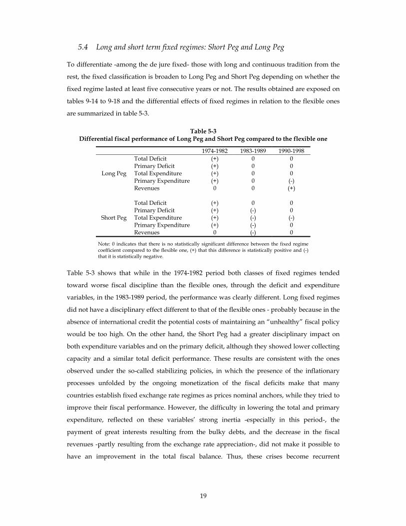
5.4 Long and short term fixed regimes: Short Peg and Long Peg

To differentiate -among the de jure fixed- those with long and continuous tradition from the

rest, the fixed classification is broaden to Long Peg and Short Peg depending on whether the

fixed regime lasted at least five consecutive years or not. The results obtained are exposed on

tables 9-14 to 9-18 and the differential effects of fixed regimes in relation to the flexible ones

are summarized in table 5-3.

Table 5-3 Differential fiscal performance of Long Peg and Short Peg compared to the flexible one

1974-1982 1983-1989 1990-1998 Total Deficit (+) 0 0 Primary Deficit (+) 0 0

Long Peg Total Expenditure (+) 0 0 Primary Expenditure (+) 0 (-) Revenues 0 0 (+)

Total Deficit (+) 0 0 Primary Deficit (+) (-) 0

Short Peg Total Expenditure (+) (-) (-) Primary Expenditure (+) (-) 0 Revenues 0 (-) 0

Note: 0 indicates that there is no statistically significant difference between the fixed regime coefficient compared to the flexible one, (+) that this difference is statistically positive and (-) that it is statistically negative.

Table 5-3 shows that while in the 1974-1982 period both classes of fixed regimes tended

toward worse fiscal discipline than the flexible ones, through the deficit and expenditure

variables, in the 1983-1989 period, the performance was clearly different. Long fixed regimes

did not have a disciplinary effect different to that of the flexible ones - probably because in the

absence of international credit the potential costs of maintaining an “unhealthy” fiscal policy

would be too high. On the other hand, the Short Peg had a greater disciplinary impact on

both expenditure variables and on the primary deficit, although they showed lower collecting

capacity and a similar total deficit performance. These results are consistent with the ones

observed under the so-called stabilizing policies, in which the presence of the inflationary

processes unfolded by the ongoing monetization of the fiscal deficits make that many

countries establish fixed exchange rate regimes as prices nominal anchors, while they tried to

improve their fiscal performance. However, the difficulty in lowering the total and primary

expenditure, reflected on these variables’ strong inertia -especially in this period-, the

payment of great interests resulting from the bulky debts, and the decrease in the fiscal

revenues -partly resulting from the exchange rate appreciation-, did not make it possible to

have an improvement in the total fiscal balance. Thus, these crises become recurrent

20

phenomena during the period. The results obtained for the 1990-1998 period are not

sufficiently clear.

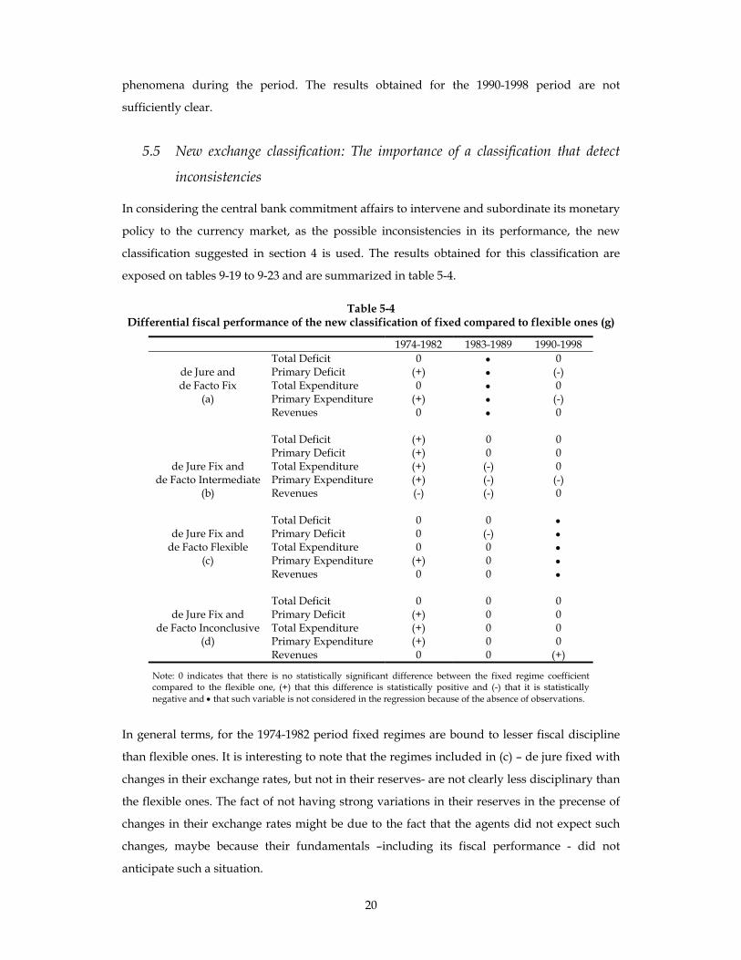
5.5 New exchange classification: The importance of a classification that detect

inconsistencies

In considering the central bank commitment affairs to intervene and subordinate its monetary

policy to the currency market, as the possible inconsistencies in its performance, the new

classification suggested in section 4 is used. The results obtained for this classification are

exposed on tables 9-19 to 9-23 and are summarized in table 5-4.

Table 5-4 Differential fiscal performance of the new classification of fixed compared to flexible ones (g)

1974-1982 1983-1989 1990-1998 Total Deficit 0 • 0

de Jure and Primary Deficit (+) • (-) de Facto Fix Total Expenditure 0 • 0

(a) Primary Expenditure (+) • (-) Revenues 0 • 0 Total Deficit (+) 0 0 Primary Deficit (+) 0 0

de Jure Fix and Total Expenditure (+) (-) 0 de Facto Intermediate Primary Expenditure (+) (-) (-)

(b) Revenues (-) (-) 0 Total Deficit 0 0 •

de Jure Fix and Primary Deficit 0 (-) • de Facto Flexible Total Expenditure 0 0 •

(c) Primary Expenditure (+) 0 • Revenues 0 0 • Total Deficit 0 0 0

de Jure Fix and Primary Deficit (+) 0 0 de Facto Inconclusive Total Expenditure (+) 0 0

(d) Primary Expenditure (+) 0 0 Revenues 0 0 (+)

Note: 0 indicates that there is no statistically significant difference between the fixed regime coefficient compared to the flexible one, (+) that this difference is statistically positive and (-) that it is statistically negative and • that such variable is not considered in the regression because of the absence of observations.

In general terms, for the 1974-1982 period fixed regimes are bound to lesser fiscal discipline

than flexible ones. It is interesting to note that the regimes included in (c) – de jure fixed with

changes in their exchange rates, but not in their reserves- are not clearly less disciplinary than

the flexible ones. The fact of not having strong variations in their reserves in the precense of

changes in their exchange rates might be due to the fact that the agents did not expect such

changes, maybe because their fundamentals –including its fiscal performance - did not

anticipate such a situation.

21

In the 1983-1989 period many countries with serious debt crises and inflationary processes

adopted de jure fixed regimes apparently with two objectives: to behave as a nominal anchor

of prices and to favor a grater fiscal discipline. Literature shows that if the government does

not have access to credit and/or had insufficient reserves, the monetary financing of the

deficits would cause an immediate depreciation independently from the exchange rate

regime. The econometric results are in line with this idea since:

• (d) - de jure fixed having stable economies, with no greater external shocks or credibility

problems – did not have a differential effect when compared to the flexible ones.

• In general terms (c) are still as disciplinary as the flexible ones due to the reasons mentioned

above.

• (b) Include most stabilizing plans of the eighties, which were not very effective in reducing

total deficits. The strong persistence of the fiscal variables in this period, the insufficient

disciplinary effect of stabilizing policies, and the recurrent re-lining of the exchange rate -

with its punishment in terms of violating a rule and losing credibility- would show that, in

those economies with a poor fiscal performance and serious inflationary problems,

governments would have to see such costs with lower weight than the ones that would

result from a true budgetary adjustment likely to make its fiscal performance consistent.

• (a) Do not have any observations. This would seem to indicate that to be defined as fixed

and behave in like manner would be highly costly at times of strong financial restrictions,

probably due to the fact that the strong inertia of fiscal variables makes it impossible to

maintain a fixed exchange rate with constant deficits and inflation.

The 1990-1998 period is, as the sixties, one of capital abundance, with flows greater than the

ones before the debt crisis. However, the incidence of fixed regimes over the fiscal

performance compared to that of the flexible ones is highly different for this period. A

possible rationalization of this uneven performance could be found in the different

characteristics of the international financial system highlighted above: growth of the bonds

and shares market, new financial instruments favoring short term positions, higher volatility

of capital flows and contagion effect. For all this, even though it is a more “calibrated” system

for rewarding a good performance, it is also so for discipline errors of private investments or

public policies once they are evident. This greater information and the opportunities make the

capitals move more easily and each time more to those opportunities more convenient,

producing a disciplinary capacity more extreme and less “sympathetic” than twenty or thirty

years ago. This evidence in its most extreme version has led Eichegreen (1994) and Obstfeld

and Rogoff (1995a) to suggest the so-called “two poles” theory, which proposes an inherent

tension between capital high mobility and countries with fixed regimes wanting to realize a

22

monetary policy with domestic objectives. According to these authors, this occurs due to the

growing fragility that the greater capital mobility imposes on the exchange commitments,

which will cause the countries to be forced to choose between flexible regimes or exchange

rate unions in the XXI century. The main obtained results show that:

• (a) Have a reversal in sign compared to those of the 1974-1982 period. This could be due to

the fact that those countries that have undergone external shocks -shown in their reserves

movement - and have been able to maintain their exchange commitment must have had a

more disciplined fiscal performance than the flexible ones.

• (b) Have a more disciplinary effect than the flexible only on the primary expenditure. This

performance –together with the possible impairment of other fundamentals- probably

favored, within the framework of highly volatile capital markets subject to panic, the

exchange rate destabilization.

• (c) Do not have any observations. This situation would show the limited current

possibilities of finding a country with de jure fixed exchange regime, which simultaneously

varies its exchange rates –violating its commitment- without being affected in its reserves’

levels.

• (d) Do not generally have a differential influence over the fiscal variables compared to the

flexible ones which, within the framework explained above, could be associated with the

fact that these stable economies with no credibility problems do not need to show a special

disciplinary performance, since they are not subject to greater external shocks. However,

they cannot relax their fiscal performance like in the seventies because they would probably

stop being stable. The underlying idea is that the exchange rate regimes have an impact on

the economic performance only when they represent a relevant restriction on the economic

policy, which is likely to happen when the country is subject to significant external shocks.

23

6 CONCLUSIONS

This paper analyzed the effect of the exchange regimes on the fiscal discipline, focusing on

the fixed and flexible difference. The results strongly suggest that such differential effect

depends on the international context, specifically on the possibility of indebtedness and the

characteristics of the international financial system. In this respect, the results suggest that the

traditional view stating that fixed regimes necessarily provide greater fiscal discipline should

be revised.

The main conclusions can be summarized in three points:

• In situations where there is originally no fiscal discipline and the authorities have the

possibility of financing with debt with relatively low costs -associated to the low probability

in the regime collapse or to the low costs in terms of the incidence of such collapse on the rest

of the economy-, as in the 1974-1982 period, fixed regimes do not provide greater discipline

per se. On the contrary, flexible ones generate greater discipline because of the immediacy of

the punishment associated to the unsustainable fiscal policy. This result is compatible with

models such as those of Alesina y Drazen (1991), Calvo (1986), Tornell y Velasco (1995a,

1995b), and Velasco (1997) according to which the presence of “weak” and divided or prone

to spend governments, in a context of abundance of credit and low initial debt percentages,

produce ceteris paribus laxer fiscal situations in countries having fixed regimes.

• In contexts with strong financing restrictions, as in the 1983-1989 period, the monetary

financing of the deficits will inevitably cause an immediate depreciation, independently from

the chosen exchange rate regime. Therefore, the disciplinary effects should not be

substantially different.

• On the contrary, in contexts of abundance of capital but where these are highly volatile

and probably subject to the contagion effect, as in the 1990-1998 period, fixed regimes

desiring to be consistent should -ceteris paribus- have a greater disciplinary effect compared

to the flexible ones to diminish the probabilities of having an exchange attack. This is in line

with what Gavin and Hausmann (1999) suggest, according to whom in the context of high

economic and financial volatility, the main factor to be protected is being solvent, as

“...solvency has as much to do with what might happen as what is expected to happen...”.

That is, “...in order to protect an economy from financial contagion it is not enough to be

solvent under existing circumstances and those that are expected to prevail; it is also

important to be solvent under more difficult circumstances that may very well be down the

road if the world financial system comes under unexpected stress.” Therefore, in the nineties,

24

greater integration, volatility and punishing capacity -associated to greater information flows

and to the bond market growth-, made the functioning of the international financial system

itself to be in charge, through its potential punishment, of obtaining an extra disciplinary

effect by those fixed regime economies desiring to remain like that. This result supports, on

the one hand, the so-called “Theory of the two poles” suggested by Eichegreen (1994) y

Obstfeld y Rogoff (1995a) and the empiric evidence found by Collins (1996) and Edwards

(1996) and, on the other hand, the “fear of pegging” phenomenon. That is to say, if in order to

possess a consistent fixed exchange rate regime a country must have an extra disciplinary

effect, greater would the incentive to adopt flexible regimes, or alternatively, those willing to

behave as fixed ones would have less incentives to define themselves as such so as not to be

subject of possible attacks to the currency.

25

7 REFERENCES

[1] Adam, C., D. Bevan y G. Chambas (2000); “Exchange rate regimes and revenue

performance in Sub-Saharan Africa”; QEH working paper Nº35.

[2] Aghevli, B., M. Khan y P. Montiel (1991); “Exchange rate policies in developing

countries: Some analytical issues”; IMF occasional paper Nº 78.

[3] Ahn, S. y P. Schmidt (1993); “Efficient estimation of models for dynamic panel data”;

Journal of econometrics, forthcoming.

[4] Alberola, E. y L. Molina (2000); “Fiscal discipline & exchange rate regimes. A case of

currency boards?”; Bank of Spain working paper Nº0006.

[5] Alesina A. y A. Drazen (1991); “Why are stabilizations delayed?”; American Economic

Review; Vol. 81: 1170-1188.

[6] Alfaro, L. (1999); “Why governments implement temporary stabilization programs”;

Journal of Applied Economics; Vol II, Nº2: 211-245.

[7] Anderson, T. y C. Hsiao (1981); “Estimation of dynamic model error components”;

Journal of American statistical association; Vol. 76: 598-606.

[8] Arellano, M. y S. Bond (1991); “Some tests of specification for panel data: Monte Carlo

evidence and an application to employment equations”; Review of Economic Studies

58: 277-297.

[9] Bachetta, P y E. Van Wincoop (1999); “Does exchange rate stability increase trade and

capital flows?”; FRBNY working paper Nº9818.

[10] Bayoumi, T. (1990); “Saving-investment correlations, immobile capital, government

policy, or endogenous behavior”, IMF staff papers.

[11] Bazzoni S. y K. Nashashibi (1994); “Exchange rate strategies and fiscal performance in

Sub-Saharan Africa”; IMF staff papers.

[12] Calvo, G. y C. Vegh (1996); “Exchange-rate-based stabilization under imperfect

credibility”, en Money, Exchange Rates, and Output. Cambridge Press.

[13] Calvo, G. y C. Reinhart (2000); “Fear of floating “; NBER working paper Nº7993.

[14] Collins, S. (1996); “On becoming more flexible: Exchange rate regimes in Latin America

and the Caribbean”; Journal of Development Economics, Vol 51.

[15] Cooper, R. (1971); “Currency devaluation in developing countries”; Princeton Essays in

International Finance, Nº86.

[16] Chang, R. (1999); “Understanding recent crises in emerging markets”. FRBA, Economic

Review, Second quarter: 6-16.

[17] ________ y A. Velasco (1998); “Financial fragility and the exchange rate regime”; NBER

working paper Nº6469.

26

[18] Devereux, M. (1999); “A simple dynamic general equilibrium analysis of the trade-off

between fixed and floating exchange rates”; mimeo.

[19] Diamond D. y P. Dybvig (1983); “Bank Runs, Deposit Insurance, and Liquidity”; Journal

of Political Economiy, Nº 91: 401-419.

[20] Edwards, S. (1996); “The determinants of the choice between fixed and flexible

exchange-rate regimes”; NBER working paper Nº5756.

[21] Eichengreen, B. (1994); International Monetary Arrangements for the 21st Century.

Washington, DC. Brookings Institution.

[22] Fischer, S. (1999); “Global markets and the global village in the 21st century: Are

international organizations prepared for the challenge?”; German Society for Foreign

Affairs, Berlin, Germany.

[23] Frenkel, J., M. Goldstein y P. Masson (1991); “Characteristics of a successful exchange

rate system”; IMF occasional paper Nº82.

[24] Frieden, J., P. Ghezzi y E. Stein (2000); “Politics and exchange rates in Latin America”;

Inter-American Development Bank research network working paper NºR-421.

[25] Gavin, M. y R. Hausmann (1999); “Preventing crisis and contagion. The domestic policy

agenda”; Conference on social protection and poverty, BID.

[26] Giavazzi, F. y M. Pagano (1988); “The advantage of tying one’s hands: EMS discipline

and central bank credibility”; European Economic Review, June.

[27] Ghosh, A., A. Gulde, J. Ostry y H. Wolf (1997); “Does the nominal exchange rate

matter?”; NBER working paper Nº5874.

[28] Greenspan, A. (1998); “The structure of the international financial system”; At the

Annual Meeting of the Securities Industry Association, Boca Raton, Florida.

[29] Helpman, E. (1981); “An exploration into the theory of exchange rate regimes”; Journal

of political economy; Vol 89.

[30] Jones, M. y M. Obstfeld (1997); “Saving, investment, and gold: A reassessment of

historical current account data”; NBER working paper Nº6103.

[31] Kamin, S. (1988); “Devaluation, exchange controls and black markets for foreign

exchange in developing countries”; BGFRS occasional paper Nº334.

[32] Krueger, A. (2002); “The evolution of emerging market capital flows: Why we need to

look again at sovereign debt restructuring”; Economics Society Dinner, Melbourne,

Australia.

[33] Krugman, P. (1979); “A balance of payments crises”; Journal of money, credit and

banking.

[34] Levy Yeyati, E. y F. Sturzenegger (2000); “Classifying exchange rate regimes: Dees vs.

words”; mimeo.

27

[35] Maddala, G. (1983); Limited Dependent and Qualitative Variables in Econometrics.

Cambridge: Cambridge University Press.

[36] Meng Q. y A. Velasco (1999); “Can capital mobility be destabilizing?”; NBER working

paper Nº7263.

[37] Mundell, R. (1960); “The monetary dynamics of international adjustment under fixed

and flexible exchange rates”; Quarterly Journal of Economics; v. LXXIV, Nº2: 227-257.

[38] __________ (1961); “ A theory of optimum currency areas”; American Economic Review;

September.

[39] Obstfeld, M. y K. Rogoff (1995a); “The mirage of fixed exchange rates”; NBER working

paper Nº5191.

[40] ______________________ (1995b); “Exchange rate dynamics redux”; Journal of Political

Economy; Vol. 103: 624-660.

[41] ______________________ (1998); “Risk and exchange rates”; NBER working paper

Nº6694.

[42] Talvi, E. y Vegh C. (2000); “Tax base variability and procyclical fiscal policy”; NBER

working paper Nº7499.

[43] Tornell, A. y P. Lane (1994); “Are windfalls a curse? A non-representative agent model

of the current account and fiscal policy”; NBER working paper Nº4839.

[44] Tornell, A. y A. Velasco (1994); “Fiscal policy and the choice of exchange rate regime”;

Inter-American Development Bank working paper Nº303.

[45] ______________________ (1995a); “Fixed versus flexible exchange rates: Which provides

more fiscal discipline?”; NBER working paper Nº5108.

[46] _____________________ (1995b); “Money-based versus exchange rate-base stabilization

with endogenous fiscal policy”; NBER working paper Nº5300.

[47] Velasco, A. (1996); “When are fixed exchange rates really fixed?”; NBER working paper

Nº5842.

[48] _________ (1997); “A model of endogenous fiscal deficits and delayed fiscal reforms”;

NBER working paper Nº6336.

[49] Weber, A. (1991); “Reputation and credibility in the European Monetary System”;

Economic Policy; Vol.12: 507-102.

[50] Wolf, H. (1997); “Regional contagion effects in emerging stock markets”; Inter Econ

working paper G-97-03: 1-18. Princeton NJ: Princeton University, Dept. of Economics,

International Finance Section.

28

8 DATA APPENDIX

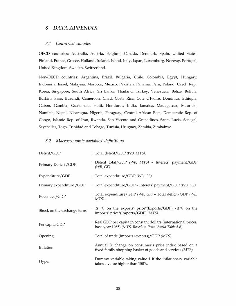
8.1 Countries’ samples

OECD countries: Australia, Austria, Belgium, Canada, Denmark, Spain, United States,

Finland, France, Greece, Holland, Ireland, Island, Italy, Japan, Luxemburg, Norway, Portugal,

United Kingdom, Sweden, Switzerland.

Non-OECD countries: Argentina, Brazil, Bulgaria, Chile, Colombia, Egypt, Hungary,

Indonesia, Israel, Malaysia, Morocco, Mexico, Pakistan, Panama, Peru, Poland, Czech Rep.,

Korea, Singapore, South Africa, Sri Lanka, Thailand, Turkey, Venezuela, Belize, Bolivia,

Burkina Faso, Burundi, Cameroon, Chad, Costa Rica, Cote d’Ivoire, Dominica, Ethiopia,

Gabon, Gambia, Guatemala, Haiti, Honduras, India, Jamaica, Madagascar, Mauricio,

Namibia, Nepal, Nicaragua, Nigeria, Paraguay, Central African Rep., Democratic Rep. of

Congo, Islamic Rep. of Iran, Rwanda, San Vicente and Grenadines, Santa Lucia, Senegal,

Seychelles, Togo, Trinidad and Tobago, Tunisia, Uruguay, Zambia, Zimbabwe.

8.2 Macroeconomic variables’ definitions

Deficit/GDP : Total deficit/GDP (WB, MTS).

Primary Deficit /GDP : Déficit total/GDP (WB, MTS) – Interets’ payment/GDP (WB, GF).

Expenditure/GDP : Total expenditure/GDP (WB, GF).

Primary expenditure /GDP : Total expenditure/GDP – Interets’ payment/GDP (WB, GF).

Revenues/GDP : Total expenditure/GDP (WB, GF) – Total deficit/GDP (WB, MTS).

Shock on the exchange terns : ∆ % on the exports’ price*(Exports/GDP) -∆% on the imports’ price*(Imports/GDP) (MTS).

Per capita GDP : Real GDP per capita in constant dollars (international prices, base year 1985) (MTS. Based on Penn World Table 5.6).

Opening : Total of trade (imports+exports)/GDP (MTS).

Inflation : Annual % change on consumer‘s price index based on a fixed family shopping basket of goods and services (MTS).

Hyper : Dummy variable taking value 1 if the inflationary variable takes a value higher than 150%.

9 TABLES APPENDIX Table 9-1

Average serial correlation of fiscal variables. 1974-1998 period.

Period Deficit/GDP Primary Deficit /GDP

Expenditure/GDP

Primary Expenditure

/GDP Revenues/GDP

t-1 0.7341 0.7544 0.9630 0.9628 0.9714 t-2 0.6461 0.6264 0.9391 0.9368 0.9582 t-3 0.5313 0.4782 0.9139 0.9086 0.9411

Obs. 1130 1080 1135 1080 1130

Table 9-2 De facto exchange classification criteria used in Levy Yeyati and Sturzenegger

(2000)

σe σ∆e σr

Inconclusive Low Low Low Flexible High High Low Dirty Floatation High High High Crawling Peg High Low High Fixed Low Low High Note: σe, σ∆e and σr are exchange rate volatility, volatility of exchange rate variations and volatility of reserves respectively.

Table 9-3 De jure exchange rate regime percentage per de facto classification

De facto classification Fixed Inter. Flexible Inconclusive

Fixed 28% 31% 11% 57% Inter. 45% 22% 26% 19% De jure classification Flexible 27% 47% 63% 24%

Total 100% 100% 100% 100%

Table 9-4 De facto exchange rate regime percentage per de jure classification

De facto classification Fixed Inter. Flex. Inconclusive Total

Fixed 6% 6% 4% 84% 100% Inter. 19% 8% 19% 54% 100% De jure

classification Flexible 8% 12% 32% 48% 100%

Table 9-5 De facto exchange rate regime percentage by de jure classification

(excepting inconclusive ones)

De facto classification Fixed Inter. Flexible Total

Fixed 39% 35% 26% 100% Inter. 42% 17% 41% 100% De jure classification Flexible 16% 22% 62% 100%

Table 9-6 Average GDP per capita per category

De facto classification Fixed Inter. Flexible Inconclusive

Fixed 1403 2942 3799 2824 Inter. 9461 4142 5017 10972 De jure classification Flexible 6339 4820 6224 4929

Table 9-7 Average inflation per category

De facto classification Fixed Inter. Flexible Inconclusive

Fixed 11.634 50.462 12.108 8.496 Inter. 6.290 58.924 20.040 8.072 De jure classification Flexible 7.585 97.967 9.973 9.007

Table 9-8

Average opening per category

De facto classification Fixed Inter. Flexible Inconclusive

Fixed 105.67 48.08 60.42 61.14 Inter. 68.13 34.75 47.75 64.61 De jure classification Flexible 55.93 47.90 40.74 54.22

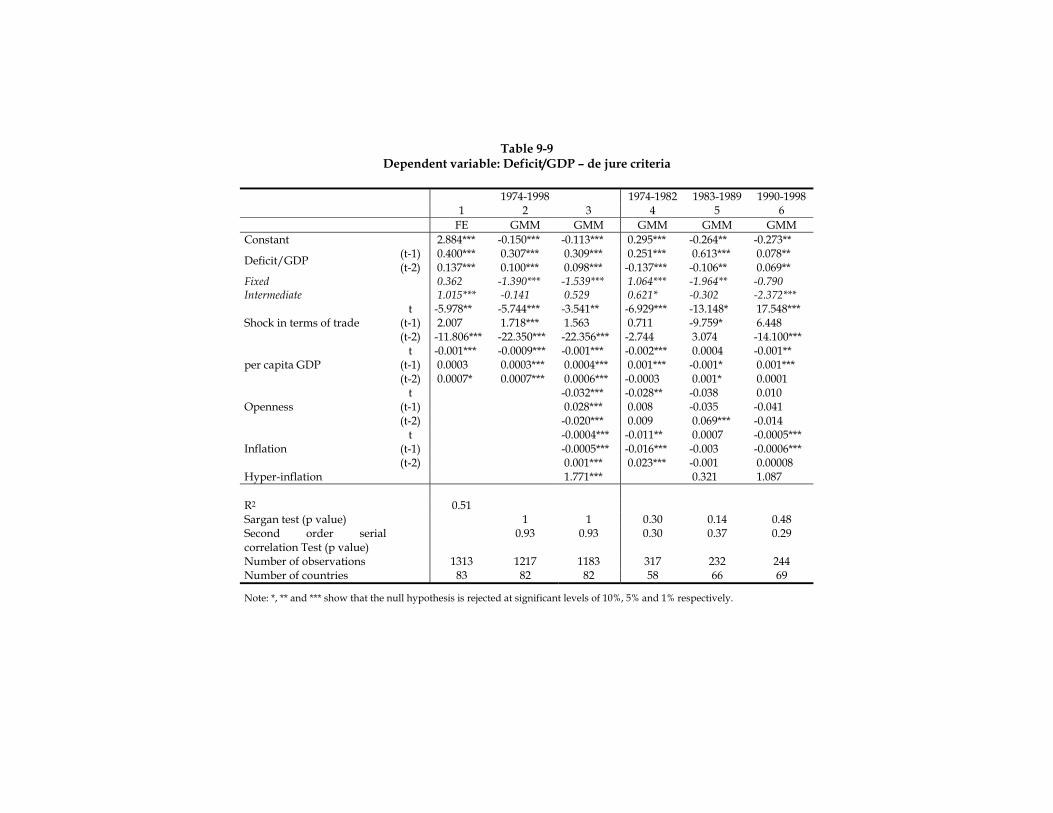
Table 9-9 Dependent variable: Deficit/GDP – de jure criteria

1974-1998 1974-1982 1983-1989 1990-1998

1 2 3 4 5 6 FE GMM GMM GMM GMM GMM

Constant 2.884*** -0.150*** -0.113*** 0.295*** -0.264** -0.273** (t-1) 0.400*** 0.307*** 0.309*** 0.251*** 0.613*** 0.078** Deficit/GDP (t-2) 0.137*** 0.100*** 0.098*** -0.137*** -0.106** 0.069**

Fixed 0.362 -1.390*** -1.539*** 1.064*** -1.964** -0.790 Intermediate 1.015*** -0.141 0.529 0.621* -0.302 -2.372***

t -5.978** -5.744*** -3.541** -6.929*** -13.148* 17.548*** (t-1) 2.007 1.718*** 1.563 0.711 -9.759* 6.448 Shock in terms of trade (t-2) -11.806*** -22.350*** -22.356*** -2.744 3.074 -14.100***

t -0.001*** -0.0009*** -0.001*** -0.002*** 0.0004 -0.001** (t-1) 0.0003 0.0003*** 0.0004*** 0.001*** -0.001* 0.001*** per capita GDP (t-2) 0.0007* 0.0007*** 0.0006*** -0.0003 0.001* 0.0001

t -0.032*** -0.028** -0.038 0.010 (t-1) 0.028*** 0.008 -0.035 -0.041 Openness (t-2) -0.020*** 0.009 0.069*** -0.014

t -0.0004*** -0.011** 0.0007 -0.0005*** (t-1) -0.0005*** -0.016*** -0.003 -0.0006*** Inflation (t-2) 0.001*** 0.023*** -0.001 0.00008

Hyper-inflation 1.771*** 0.321 1.087 R2 0.51 Sargan test (p value) 1 1 0.30 0.14 0.48 Second order serial correlation Test (p value)

0.93 0.93 0.30 0.37 0.29

Number of observations 1313 1217 1183 317 232 244 Number of countries 83 82 82 58 66 69

Note: *, ** and *** show that the null hypothesis is rejected at significant levels of 10%, 5% and 1% respectively.

32

Table 9-10 Dependent variable: Primary Deficit/GDP – de jure criteria

1974-1998 1974-1982 1983-1989 1990-1998

1 2 3 4 5 6 FE GMM GMM GMM GMM GMM

Constant 0.798 -0.244*** -0.219*** 0.055 -0.229** -0.081 (t-1) 0.445*** 0.364*** 0.370*** 0.314*** 0.572*** 0.291*** Primary deficit/GDP (t-2) 0.133*** 0.098*** 0.101*** -0.155*** -0.125** 0.113***

Fixed 0.931*** -0.323 -1.270*** 1.128*** -1.310 0.002 Intermediate 1.485*** 1.648*** 1.375*** 0.783*** 0.213 -1.635**

t -11.005*** -10.825*** -11.949*** -12.149*** -20.891*** 10.166** (t-1) 2.574 1.859** -3.226* -1.241 -12.583** -9.228** Shock in terms of trade (t-2) -14.083*** -28.693*** -25.973*** -3.116* -0.983 -5.301

t -0.001*** -0.0001 0.00002 -0.001*** 0.00008 -0.001*** (t-1) 0.0004 -0.0003** -0.0002* 0.001** -0.0008 0.001*** per capita GDP (t-2) 0.0006* 0.0009*** 0.0008*** -0.0002 0.0009 0.001**

t -0.042*** -0.018* -0.029 -0.031 (t-1) 0.062*** 0.021 0.007 0.041** Openness (t-2) -0.049*** 0.001 0.021 -0.057**

t -0.0003*** -0.017*** 0.0003 -0.0005*** (t-1) -0.0004*** -0.017*** -0.005 -0.0007*** Inflation (t-2) 0.001*** 0.022*** -0.002 0.00006

Hyper-inflation 0.910 1.975 -2.460** R2 0.53 Sargan test (p value) 1 1 0.44 0.37 0.84 Second order serial correlation Test (p value)

0.93 0.69 0.29 0.16 0.13

Number of observations 1176 1076 1053 289 214 224 Number of countries 82 77 77 54 61 62

Note: *, ** and *** show that the null hypothesis is rejected at significant levels of 10%, 5% and 1% respectively.

33

Table 9-11 Dependent variable: Expenditure/GDP – de jure criteria

1974-1998 1974-1982 1983-1989 1990-1998

1 2 3 4 5 6 FE GMM GMM GMM GMM GMM

Constant 7.645*** 0.020** 0.016** 0.699*** -0.363*** -0.179** (t-1) 0.637*** 0.509*** 0.485*** 0.221*** 0.530*** 0.393*** Expenditure/GDP (t-2) 0.103*** 0.061*** 0.070*** -0.066*** 0.075* -0.007

Fixed -0.288 -0.775*** -0.521** 1.670*** -1.457 -1.237** Intermediate 0.177 -0.176 -0.017 0.701*** -1.095 -1.475***

t -2.334 -1.677 -0.654 -11.489*** -20.541*** 3.900 (t-1) 8.954*** 8.572*** 8.147*** 1.735 -4.123 5.910*** Shock in terms of trade (t-2) -11.709*** -24.088*** -22.630*** -3.619** 7.140 1.336

t -0.001*** -0.002*** -0.002*** -0.002*** -0.0006 -0.002*** (t-1) 0.001** 0.001*** 0.002*** 0.001*** -0.0004 0.001*** per capita GDP (t-2) 0.0003 0.00008 0.0001 0.0001 0.001* 0.0002

t -0.017*** -0.010 -0.035 0.014 (t-1) 0.063*** 0.052*** -0.018 -0.022 Openness (t-2) -0.012*** 0.004 0.052** -0.067***

t 0.0001 -0.027*** -0.00005 -0.0006*** (t-1) 0.00005* -0.010** 0.001 -0.00009 Inflation (t-2) 0.0005*** 0.024*** -0.0007 0.00007*

Hyper-inflation 1.598* -0.548 4.357 R2 0.93 Sargan test (p value) 1 1 0.18 0.02 0.40 Second order serial correlation Test (p value)

0.16 0.31 0.13 0.44 0.27

Number of observations 1311 1216 1180 330 228 250 Number of countries 83 83 83 61 65 67

Note: *, ** and *** show that the null hypothesis is rejected at significant levels of 10%, 5% and 1% respectively.

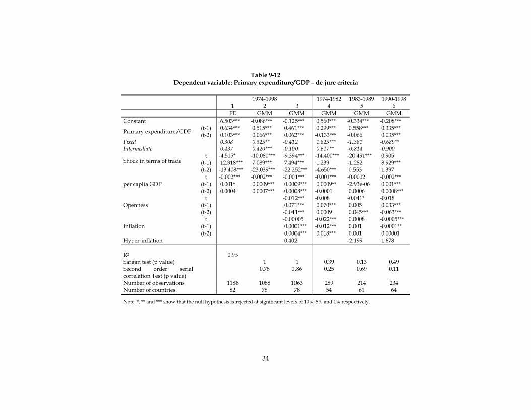
34

Table 9-12 Dependent variable: Primary expenditure/GDP – de jure criteria

1974-1998 1974-1982 1983-1989 1990-1998

1 2 3 4 5 6 FE GMM GMM GMM GMM GMM

Constant 6.503*** -0.086*** -0.125*** 0.560*** -0.334*** -0.208*** (t-1) 0.634*** 0.515*** 0.461*** 0.299*** 0.558*** 0.335*** Primary expenditure/GDP (t-2) 0.103*** 0.066*** 0.062*** -0.133*** -0.066 0.035***

Fixed 0.308 0.325** -0.412 1.825*** -1.381 -0.689** Intermediate 0.437 0.420*** -0.100 0.617** -0.814 -0.900

t -4.515* -10.080*** -9.394*** -14.400*** -20.491*** 0.905 (t-1) 12.318*** 7.089*** 7.494*** 1.239 -1.282 8.929*** Shock in terms of trade (t-2) -13.408*** -23.039*** -22.252*** -4.650*** 0.553 1.397

t -0.002*** -0.002*** -0.001*** -0.001*** -0.0002 -0.002*** (t-1) 0.001* 0.0009*** 0.0009*** 0.0009** -2.93e-06 0.001*** per capita GDP (t-2) 0.0004 0.0007*** 0.0008*** -0.0001 0.0006 0.0008***

t -0.012*** -0.008 -0.041* -0.018 (t-1) 0.071*** 0.070*** 0.005 0.033*** Openness (t-2) -0.041*** 0.0009 0.045*** -0.063***

t -0.00005 -0.022*** 0.0008 -0.0005*** (t-1) 0.0001*** -0.012*** 0.001 -0.0001** Inflation (t-2) 0.0004*** 0.018*** 0.001 0.00001

Hyper-inflation 0.402 -2.199 1.678 R2 0.93 Sargan test (p value) 1 1 0.39 0.13 0.49 Second order serial correlation Test (p value)

0.78 0.86 0.25 0.69 0.11

Number of observations 1188 1088 1063 289 214 234 Number of countries 82 78 78 54 61 64

Note: *, ** and *** show that the null hypothesis is rejected at significant levels of 10%, 5% and 1% respectively.

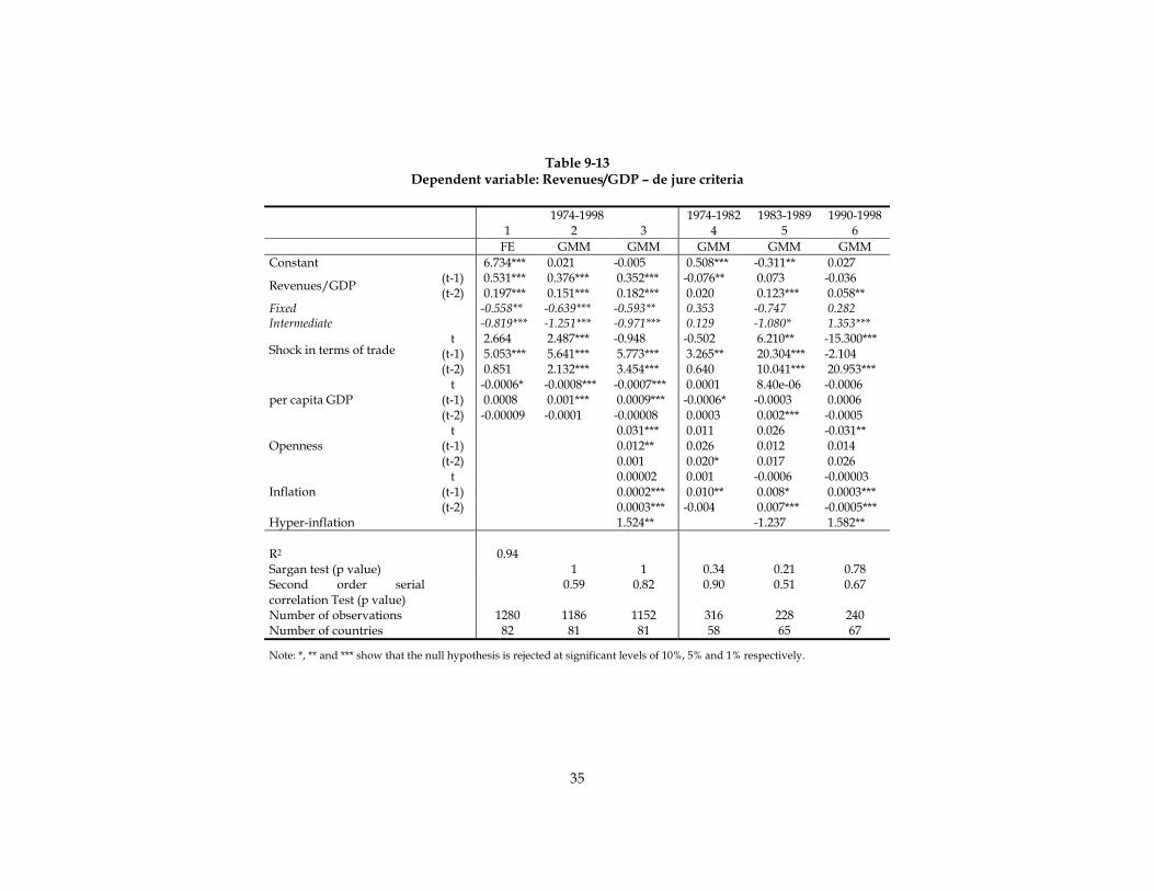
35

Table 9-13 Dependent variable: Revenues/GDP – de jure criteria

1974-1998 1974-1982 1983-1989 1990-1998

1 2 3 4 5 6 FE GMM GMM GMM GMM GMM

Constant 6.734*** 0.021 -0.005 0.508*** -0.311** 0.027 (t-1) 0.531*** 0.376*** 0.352*** -0.076** 0.073 -0.036 Revenues/GDP (t-2) 0.197*** 0.151*** 0.182*** 0.020 0.123*** 0.058**

Fixed -0.558** -0.639*** -0.593** 0.353 -0.747 0.282 Intermediate -0.819*** -1.251*** -0.971*** 0.129 -1.080* 1.353***

t 2.664 2.487*** -0.948 -0.502 6.210** -15.300*** (t-1) 5.053*** 5.641*** 5.773*** 3.265** 20.304*** -2.104 Shock in terms of trade (t-2) 0.851 2.132*** 3.454*** 0.640 10.041*** 20.953***

t -0.0006* -0.0008*** -0.0007*** 0.0001 8.40e-06 -0.0006 (t-1) 0.0008 0.001*** 0.0009*** -0.0006* -0.0003 0.0006 per capita GDP (t-2) -0.00009 -0.0001 -0.00008 0.0003 0.002*** -0.0005

t 0.031*** 0.011 0.026 -0.031** (t-1) 0.012** 0.026 0.012 0.014 Openness (t-2) 0.001 0.020* 0.017 0.026

t 0.00002 0.001 -0.0006 -0.00003 (t-1) 0.0002*** 0.010** 0.008* 0.0003*** Inflation (t-2) 0.0003*** -0.004 0.007*** -0.0005***

Hyper-inflation 1.524** -1.237 1.582** R2 0.94 Sargan test (p value) 1 1 0.34 0.21 0.78 Second order serial correlation Test (p value)

0.59 0.82 0.90 0.51 0.67

Number of observations 1280 1186 1152 316 228 240 Number of countries 82 81 81 58 65 67

Note: *, ** and *** show that the null hypothesis is rejected at significant levels of 10%, 5% and 1% respectively.

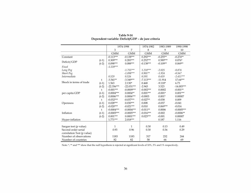
36

Table 9-14 Dependent variable: Deficit/GDP – de jure criteria

1974-1998 1974-1982 1983-1989 1990-1998

3 7 8 9 10 GMM GMM GMM GMM GMM

Constant -0.113*** -0.138*** 0.292*** -0.255** -0.274** (t-1) 0.309*** 0.283*** 0.252*** 0.589*** 0.076* Deficit/GDP (t-2) 0.098*** 0.088*** -0.138*** -0.109** 0.069**

Fixed -1.539*** Long Peg -1.755*** 1.218*** -2.025 -0.874 Short Peg -1.898*** 0.901** -1.924 -0.567 Intermediate 0.529 0.526 0.591 0.419 -2.411***

t -3.541** -3.349*** -7.113*** -11.914 17.64*** (t-1) 1.563 2.130* 0.468 -9.118* 6.73 Shock in terms of trade (t-2) -22.356*** -22.031*** -2.943 3.523 -14.003***

t -0.001*** -0.0009*** -0.002*** 0.0002 -0.001** (t-1) 0.0004*** 0.0004** 0.001*** -0.001* 0.001*** per capita GDP (t-2) 0.0006*** 0.0006*** -0.0003 0.001* 0.00007

t -0.032*** -0.037*** -0.027** -0.038 0.009 (t-1) 0.028*** 0.030*** 0.008 -0.037 -0.041 Openness (t-2) -0.020*** -0.021*** 0.010 0.069*** -0.014

t -0.0004*** -0.0004*** -0.011** 0.0006 -0.0005*** (t-1) -0.0005*** -0.0005*** -0.016*** -0.002 -0.0006** Inflation (t-2) 0.001*** 0.0001*** 0.023*** -0.001 0.00007

Hyper-inflation 1.771*** 2.018*** 0.187 1.116 Sargan test (p value) 1 1 0.30 0.13 0.49 Second order serial correlation Test (p value)

0.93 0.96 0.30 0.36 0.29

Number of observations 1183 1183 317 232 244 Number of countries 82 82 58 66 69

Note: *, ** and *** show that the null hypothesis is rejected at significant levels of 10%, 5% and 1% respectively.

37

Table 9-15 Dependent variable: Primary deficit/GDP – de jure criteria

1974-1998 1974-1982 1983-1989 1990-1998

3 7 8 9 10 GMM GMM GMM GMM GMM

Constant -0.219*** -0.196*** 0.057 -0.201* -0.072 (t-1) 0.370*** 0.377*** 0.317*** 0.613*** 0.259*** Primary deficit/GDP (t-2) 0.101*** 0.104*** -0.154*** -0.102** 0.113***

Fixed -1.270*** Long Peg -1.727*** 1.167*** -0.025 -0.301 Short Peg -1.255 1.113*** -3.325*** 0.801 Intermediate 1.375*** 1.637*** 0.789*** -0.095 -1.803***

t -11.949*** -5.390 -12.085*** -21.271*** 10.127** (t-1) -3.226* -0.234 -1.204 -12.102** -7.935* Shock in terms of trade (t-2) -25.973*** -26.061*** -3.031* 0.166 -5.125

t 0.00002 -0.0006*** -0.001*** 0.003 -0.001*** (t-1) -0.0002* 0.00008 0.001** -0.0009 0.001*** per capita GDP (t-2) 0.0008*** 0.0008*** -0.0002 0.0006 0.001**

t -0.042*** -0.036*** -0.018* -0.026 -0.028 (t-1) 0.062*** 0.062*** 0.021 0.006 0.034** Openness (t-2) -0.049*** -0.050*** 0.002 0.026 -0.054**

t -0.0003*** -0.0004*** -0.017*** 0.0002 -0.0005*** (t-1) -0.0004*** -0.0004*** -0.017*** -0.004 -0.0007*** Inflation (t-2) 0.001*** 0.001*** 0.022*** -0.001 0.00004

Hyper-inflation 0.910 2.399** 1.823 -2.461** Sargan test (p value) 1 1 0.45 0.36 0.83 Second order serial correlation Test (p value)

0.69 0.35 0.30 0.20 0.13

Number of observations 1053 1053 289 214 224 Number of countries 77 77 54 61 62

Note: *, ** and *** show that the null hypothesis is rejected at significant levels of 10%, 5% and 1% respectively.

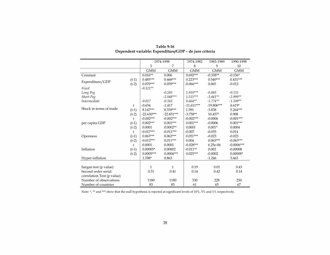
38

Table 9-16 Dependent variable: Expenditure/GDP – de jure criteria

1974-1998 1974-1982 1983-1989 1990-1998

3 7 8 9 10 GMM GMM GMM GMM GMM

Constant 0.016** 0.006 0.692*** -0.338** -0.156* (t-1) 0.485*** 0.468*** 0.223*** 0.540*** 0.431*** Expenditure/GDP (t-2) 0.070*** 0.059*** -0.066*** 0.065 -0.012

Fixed -0.521** Long Peg -0.185 1.910*** -0.885 -0.131 Short Peg -2.048*** 1.515*** -3.441** -2.999** Intermediate -0.017 -0.165 0.664** -1.774** -1.109**

t -0.654 -1.417 -11.611*** -19.806*** 4.619* (t-1) 8.147*** 8.339*** 1.591 -3.838 5.264*** Shock in terms of trade (t-2) -22.630*** -22.851*** -3.758** 10.457* 0.908

t -0.002*** -0.002*** -0.002*** -0.0006 -0.001*** (t-1) 0.002*** 0.001*** 0.001*** -0.0006 0.001*** per capita GDP (t-2) 0.0001 0.0002** 0.0001 0.001* 0.0004

t -0.017*** -0.011*** -0.007 -0.035 0.014 (t-1) 0.063*** 0.063*** 0.051*** -0.023 -0.023 Openness (t-2) -0.012*** 0.011*** 0.004 0.063*** -0.063***

t 0.0001 0.0001 -0.028*** 6.25e-06 -0.0006*** (t-1) 0.00005* 0.00002 -0.011** 0.002 -0.00008 Inflation (t-2) 0.0005*** 0.0004*** 0.025*** -0.0002 0.00008*

Hyper-inflation 1.598* 0.863 -1.246 3.663 Sargan test (p value) 1 1 0.19 0.01 0.43 Second order serial correlation Test (p value)

0.31 0.41 0.14 0.42 0.14

Number of observations 1180 1180 330 228 250 Number of countries 83 83 61 65 67

Note: *, ** and *** show that the null hypothesis is rejected at significant levels of 10%, 5% and 1% respectively.

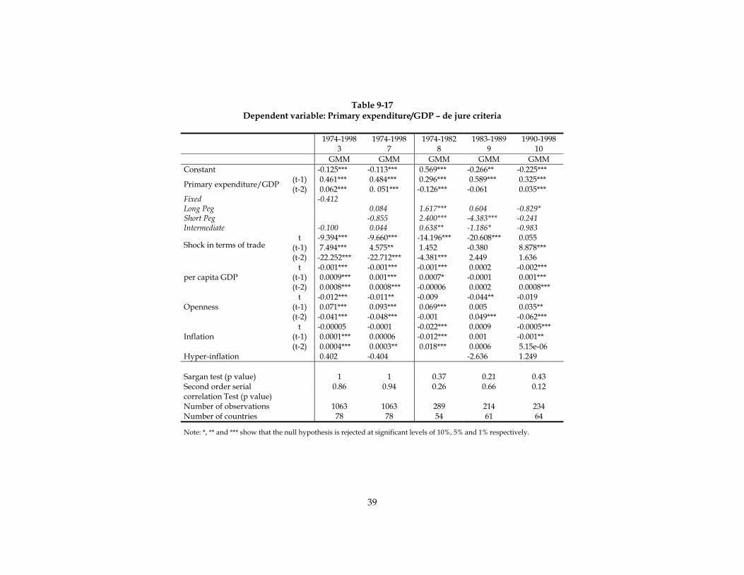
39

Table 9-17 Dependent variable: Primary expenditure/GDP – de jure criteria

1974-1998 1974-1998 1974-1982 1983-1989 1990-1998

3 7 8 9 10 GMM GMM GMM GMM GMM

Constant -0.125*** -0.113*** 0.569*** -0.266** -0.225*** (t-1) 0.461*** 0.484*** 0.296*** 0.589*** 0.325*** Primary expenditure/GDP (t-2) 0.062*** 0. 051*** -0.126*** -0.061 0.035***

Fixed -0.412 Long Peg 0.084 1.617*** 0.604 -0.829* Short Peg -0.855 2.400*** -4.383*** -0.241 Intermediate -0.100 0.044 0.638** -1.186* -0.983

t -9.394*** -9.660*** -14.196*** -20.608*** 0.055 (t-1) 7.494*** 4.575** 1.452 -0.380 8.878*** Shock in terms of trade (t-2) -22.252*** -22.712*** -4.381*** 2.449 1.636

t -0.001*** -0.001*** -0.001*** 0.0002 -0.002*** (t-1) 0.0009*** 0.001*** 0.0007* -0.0001 0.001*** per capita GDP (t-2) 0.0008*** 0.0008*** -0.00006 0.0002 0.0008***

t -0.012*** -0.011** -0.009 -0.044** -0.019 (t-1) 0.071*** 0.093*** 0.069*** 0.005 0.035** Openness (t-2) -0.041*** -0.048*** -0.001 0.049*** -0.062***

t -0.00005 -0.0001 -0.022*** 0.0009 -0.0005*** (t-1) 0.0001*** 0.00006 -0.012*** 0.001 -0.001** Inflation (t-2) 0.0004*** 0.0003** 0.018*** 0.0006 5.15e-06

Hyper-inflation 0.402 -0.404 -2.636 1.249 Sargan test (p value) 1 1 0.37 0.21 0.43 Second order serial correlation Test (p value)

0.86 0.94 0.26 0.66 0.12

Number of observations 1063 1063 289 214 234 Number of countries 78 78 54 61 64

Note: *, ** and *** show that the null hypothesis is rejected at significant levels of 10%, 5% and 1% respectively.

40

Table 9-18 Dependent variable: Revenues/GDP – de jure criteria

1974-1998 1974-1998 1974-1982 1983-1989 1990-1998

3 7 8 9 10 GMM GMM GMM GMM GMM

Constant -0.005 0.018 0.500*** -0.308** 0.046 (t-1) 0.352*** 0.324*** -0.069** 0.069 -0.099** Revenues/GDP (t-2) 0.182*** 0.166*** 0.164 0.123** 0.019

Fixed -0.593** Long Peg -0.482 0.214 -0.676 0.584** Short Peg -1.167** 0.490 -1.035** -0.856 Intermediate -0.971*** -0.749* 0.151 -1.163* 1.400***

t -0.948 -2.174 -0.413 6.295** -15.012*** (t-1) 5.773*** 5.945*** 3.260** 20.283*** -4.278 Shock in terms of trade (t-2) 3.454*** 2.819** 0.832 10.202*** 20.872***

t -0.0007*** -0.0006*** 0.0001 0.0002 -0.0006 (t-1) 0.0009*** 0.0008*** -0.0006* -0.003 0.0003 per capita GDP (t-2) -0.00008 -0.00006 0.0003 0.001*** -0.0002

t 0.031*** 0.033*** 0.011 0.027 -0.034** (t-1) 0.012** 0.15*** 0.025 0.011 0.019* Openness (t-2) 0.001 0.002 0.018** 0.018 0.028

t 0.00002 0.00003 0.0007 -0.0005 -0.00001 (t-1) 0.0002*** 0.0002*** 0.010** 0.008** 0.0003*** Inflation (t-2) 0.0003*** 0.0003*** -0.003 0.007*** -0.0005***

Hyper-inflation 1.524** 1.328 -1.274 1.547 Sargan test (p value) 1 1 0.35 0.21 0.65 Second order serial correlation Test (p value)

0.82 0.72 0.86 0.51 0.64

Number of observations 1152 1152 316 228 240 Number of countries 81 81 58 65 67

Note: *, ** and *** show that the null hypothesis is rejected at significant levels of 10%, 5% and 1% respectively.

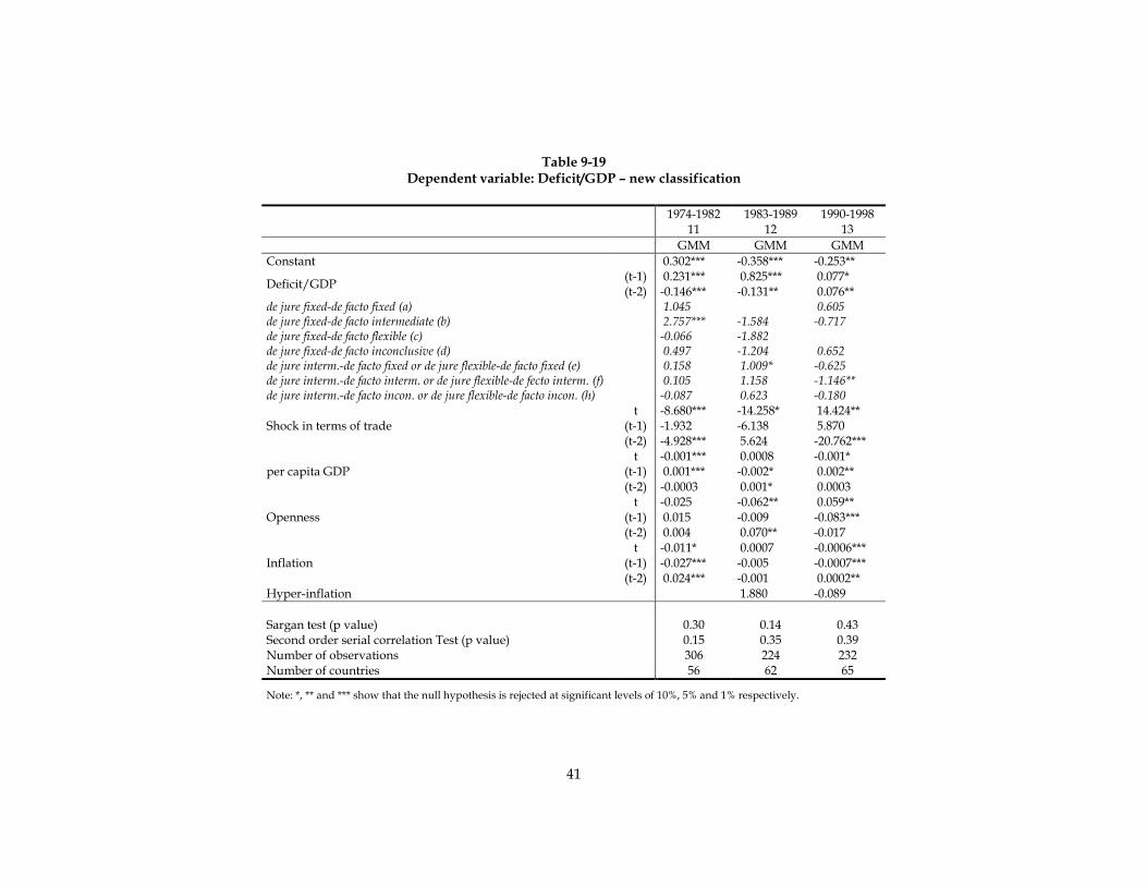
41

Table 9-19 Dependent variable: Deficit/GDP – new classification

1974-1982 1983-1989 1990-1998 11 12 13 GMM GMM GMM Constant 0.302*** -0.358*** -0.253**

(t-1) 0.231*** 0.825*** 0.077* Deficit/GDP (t-2) -0.146*** -0.131** 0.076** de jure fixed-de facto fixed (a) 1.045 0.605 de jure fixed-de facto intermediate (b) 2.757*** -1.584 -0.717 de jure fixed-de facto flexible (c) -0.066 -1.882 de jure fixed-de facto inconclusive (d) 0.497 -1.204 0.652 de jure interm.-de facto fixed or de jure flexible-de facto fixed (e) 0.158 1.009* -0.625 de jure interm.-de facto interm. or de jure flexible-de fecto interm. (f) 0.105 1.158 -1.146** de jure interm.-de facto incon. or de jure flexible-de facto incon. (h) -0.087 0.623 -0.180

t -8.680*** -14.258* 14.424** (t-1) -1.932 -6.138 5.870 Shock in terms of trade (t-2) -4.928*** 5.624 -20.762***

t -0.001*** 0.0008 -0.001* (t-1) 0.001*** -0.002* 0.002** per capita GDP (t-2) -0.0003 0.001* 0.0003

t -0.025 -0.062** 0.059** (t-1) 0.015 -0.009 -0.083*** Openness (t-2) 0.004 0.070** -0.017

t -0.011* 0.0007 -0.0006*** (t-1) -0.027*** -0.005 -0.0007*** Inflation (t-2) 0.024*** -0.001 0.0002**

Hyper-inflation 1.880 -0.089 Sargan test (p value) 0.30 0.14 0.43 Second order serial correlation Test (p value) 0.15 0.35 0.39 Number of observations 306 224 232 Number of countries 56 62 65

Note: *, ** and *** show that the null hypothesis is rejected at significant levels of 10%, 5% and 1% respectively.

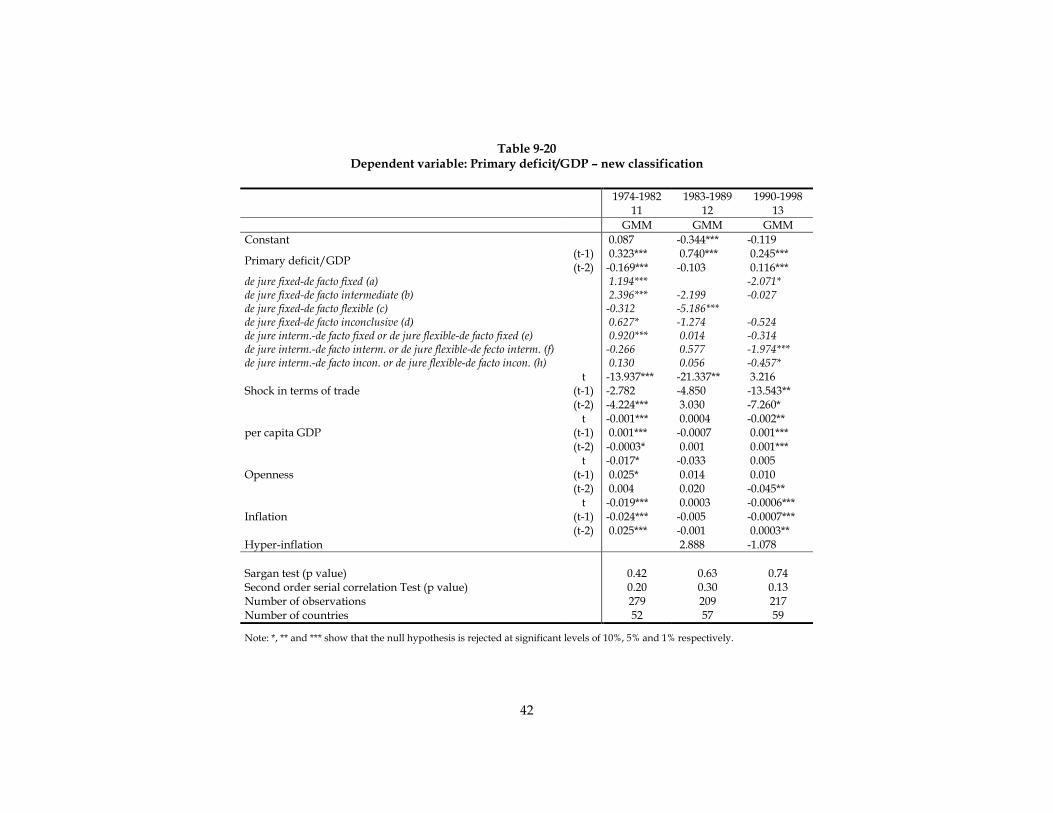
42

Table 9-20 Dependent variable: Primary deficit/GDP – new classification

1974-1982 1983-1989 1990-1998

11 12 13 GMM GMM GMM

Constant 0.087 -0.344*** -0.119 (t-1) 0.323*** 0.740*** 0.245*** Primary deficit/GDP (t-2) -0.169*** -0.103 0.116***

de jure fixed-de facto fixed (a) 1.194*** -2.071* de jure fixed-de facto intermediate (b) 2.396*** -2.199 -0.027 de jure fixed-de facto flexible (c) -0.312 -5.186*** de jure fixed-de facto inconclusive (d) 0.627* -1.274 -0.524 de jure interm.-de facto fixed or de jure flexible-de facto fixed (e) 0.920*** 0.014 -0.314 de jure interm.-de facto interm. or de jure flexible-de fecto interm. (f) -0.266 0.577 -1.974*** de jure interm.-de facto incon. or de jure flexible-de facto incon. (h) 0.130 0.056 -0.457*

t -13.937*** -21.337** 3.216 (t-1) -2.782 -4.850 -13.543** Shock in terms of trade (t-2) -4.224*** 3.030 -7.260*

t -0.001*** 0.0004 -0.002** (t-1) 0.001*** -0.0007 0.001*** per capita GDP (t-2) -0.0003* 0.001 0.001***

t -0.017* -0.033 0.005 (t-1) 0.025* 0.014 0.010 Openness (t-2) 0.004 0.020 -0.045**

t -0.019*** 0.0003 -0.0006*** (t-1) -0.024*** -0.005 -0.0007*** Inflation (t-2) 0.025*** -0.001 0.0003**

Hyper-inflation 2.888 -1.078 Sargan test (p value) 0.42 0.63 0.74 Second order serial correlation Test (p value) 0.20 0.30 0.13 Number of observations 279 209 217 Number of countries 52 57 59

Note: *, ** and *** show that the null hypothesis is rejected at significant levels of 10%, 5% and 1% respectively.

43

Table 9-21 Dependent variable: Expenditure/GDP – new classification

1974-1982 1983-1989 1990-1998

11 12 13 GMM GMM GMM

Constant 0.751*** -0.364*** -0.119 (t-1) 0.144*** 0.476*** 0.354*** Expenditure/GDP (t-2) -0.088*** 0.100** 0.019

de jure fixed-de facto fixed (a) 0.626 0.192 de jure fixed-de facto intermediate (b) 1.091** -2.075* -1.392 de jure fixed-de facto flexible (c) 0.682 0.605 de jure fixed-de facto inconclusive (d) 0.752* -0.598 -0.078 de jure interm.-de facto fixed or de jure flexible-de facto fixed (e) -0.554* -0.297 0.515 de jure interm.-de facto interm. or de jure flexible-de fecto interm. (f) -0.038 0.639 0.524 de jure interm.-de facto incon. or de jure flexible-de facto incon. (h) -0.695*** -0.179 -0.327

t -12.290*** -17.400*** 4.330* (t-1) -0.876 -2.518 7.676*** Shock in terms of trade (t-2) -4.970*** 6.948 -7.922**

t -0.002*** -0.0005 -0.002*** (t-1) 0.001*** -0.0008 0.001** per capita GDP (t-2) 0.0001 0.002** 0.0002

t -0.017 -0.007 0.004 (t-1) 0.061*** -0.042 -0.009 Openness (t-2) -0.003 0.059** -0.032*

t -0.034*** -0.0002 -0.0004*** (t-1) -0.015*** -0.00005 -0.0001*** Inflation (t-2) 0.028*** -0.0012 -0.00001

Hyper-inflation 0.846 1.585 Sargan test (p value) 0.07 0.01 0.59 Second order serial correlation Test (p value) 0.11 0.49 0.07 Number of observations 319 220 238 Number of countries 59 61 63

Note: *, ** and *** show that the null hypothesis is rejected at significant levels of 10%, 5% and 1% respectively.

44

Table 9-22 Dependent variable: Primary expenditure/GDP – new classification

1974-1982 1983-1989 1990-1998

11 12 13 GMM GMM GMM

Constant 0.491*** -0.434*** -0.105* (t-1) 0.234*** 0.469*** 0.429*** Primary expenditure/GDP (t-2) -0.144*** -0.036 0.054***

de jure fixed-de facto fixed (a) 1.123*** -1.458** de jure fixed-de facto intermediate (b) 1.081** -1.476* -1.813*** de jure fixed-de facto flexible (c) 0.866** -0.721 de jure fixed-de facto inconclusive (d) 1.071** -0.545 0.094 de jure interm.-de facto fixed or de jure flexible-de facto fixed (e) 0.543 -0.126 0.655** de jure interm.-de facto interm. or de jure flexible-de fecto interm. (f) -0.587 0.805 -0.544 de jure interm.-de facto incon. or de jure flexible-de facto incon. (h) -0.292 0.056 -0.746***

t -16.577*** -14.726*** 2.945 (t-1) -0.739 3.663 13.518*** Shock in terms of trade (t-2) -5.107*** 3.784 -2.153

t -0.001*** -0.00001 -0.002*** (t-1) 0.0009* -0.0002 0.001*** per capita GDP (t-2) -0.0001 0.0006 0.0006***

t -0.007 -0.028 -0.033* (t-1) 0.074*** -0.017 0.047*** Openness (t-2) 0.002 0.047*** -0.041***

t -0.023*** 0.001 -0.0004*** (t-1) -0.019*** 0.002 -0.00001 Inflation (t-2) 0.021*** 0.002 0.00006**

Hyper-inflation -3.064 0.434 Sargan test (p value) 0.10 0.03 0.58 Second order serial correlation Test (p value) 0.22 0.45 0.07 Number of observations 279 209 227 Number of countries 52 57 61

Note: *, ** and *** show that the null hypothesis is rejected at significant levels of 10%, 5% and 1% respectively.

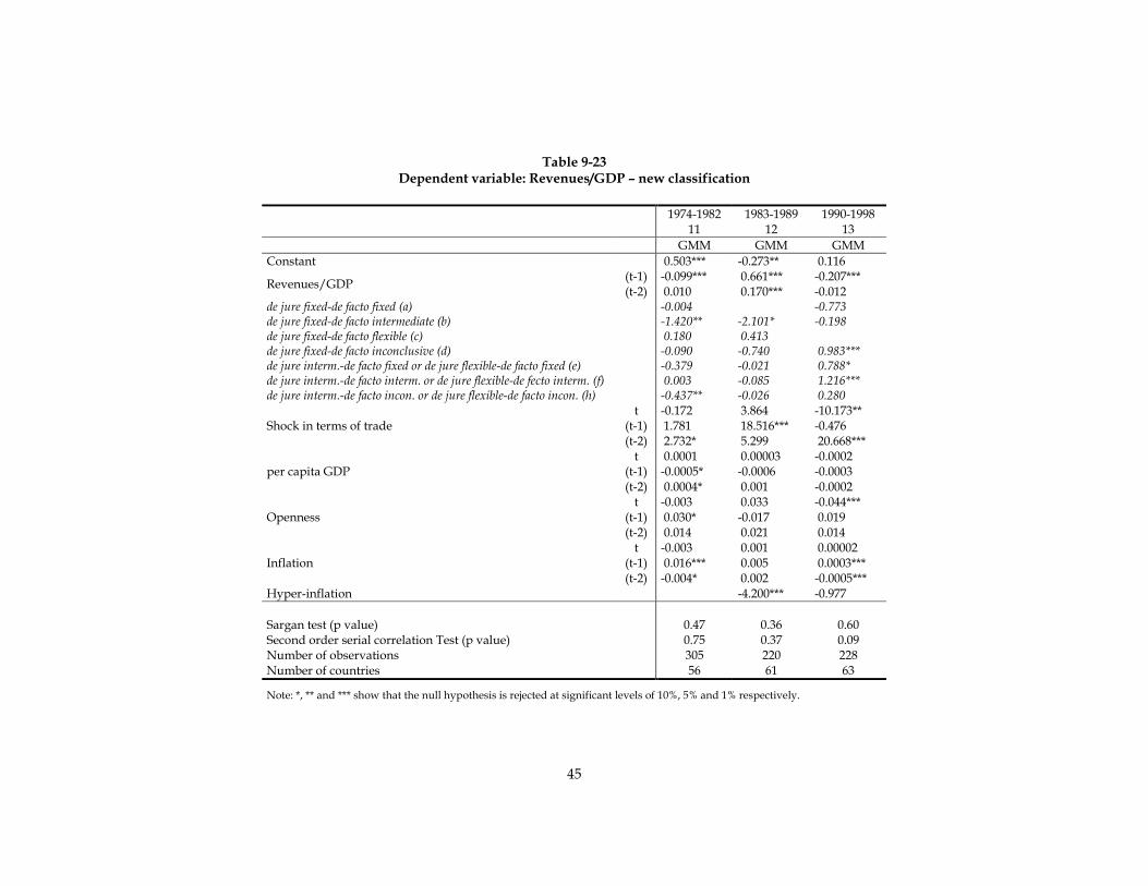
45

Table 9-23 Dependent variable: Revenues/GDP – new classification

1974-1982 1983-1989 1990-1998

11 12 13 GMM GMM GMM

Constant 0.503*** -0.273** 0.116 (t-1) -0.099*** 0.661*** -0.207*** Revenues/GDP (t-2) 0.010 0.170*** -0.012

de jure fixed-de facto fixed (a) -0.004 -0.773 de jure fixed-de facto intermediate (b) -1.420** -2.101* -0.198 de jure fixed-de facto flexible (c) 0.180 0.413 de jure fixed-de facto inconclusive (d) -0.090 -0.740 0.983*** de jure interm.-de facto fixed or de jure flexible-de facto fixed (e) -0.379 -0.021 0.788* de jure interm.-de facto interm. or de jure flexible-de fecto interm. (f) 0.003 -0.085 1.216*** de jure interm.-de facto incon. or de jure flexible-de facto incon. (h) -0.437** -0.026 0.280

t -0.172 3.864 -10.173** (t-1) 1.781 18.516*** -0.476 Shock in terms of trade (t-2) 2.732* 5.299 20.668***

t 0.0001 0.00003 -0.0002 (t-1) -0.0005* -0.0006 -0.0003 per capita GDP (t-2) 0.0004* 0.001 -0.0002

t -0.003 0.033 -0.044*** (t-1) 0.030* -0.017 0.019 Openness (t-2) 0.014 0.021 0.014

t -0.003 0.001 0.00002 (t-1) 0.016*** 0.005 0.0003*** Inflation (t-2) -0.004* 0.002 -0.0005***

Hyper-inflation -4.200*** -0.977 Sargan test (p value) 0.47 0.36 0.60 Second order serial correlation Test (p value) 0.75 0.37 0.09 Number of observations 305 220 228 Number of countries 56 61 63

Note: *, ** and *** show that the null hypothesis is rejected at significant levels of 10%, 5% and 1% respectively.