Exchange Rate Predictability and State-of-the-Art Models · Exchange Rate Predictability ... power for future exchange rate movements in advanced economies than for such ... variables

Exchange Rate Predictability and State-of-the-Art Models Pinar Yeşin

SNB Working Papers 2/2016

Disclaimer The views expressed in this paper are those of the author(s) and do not necessarily represent those of the Swiss National Bank. Working Papers describe research in progress. Their aim is to elicit comments and to further debate. copyright© The Swiss National Bank (SNB) respects all third-party rights, in particular rights relating to works protected by copyright (infor-mation or data, wordings and depictions, to the extent that these are of an individual character). SNB publications containing a reference to a copyright (© Swiss National Bank/SNB, Zurich/year, or similar) may, under copyright law, only be used (reproduced, used via the internet, etc.) for non-commercial purposes and provided that the source is mentioned. Their use for commercial purposes is only permitted with the prior express consent of the SNB. General information and data published without reference to a copyright may be used without mentioning the source. To the extent that the information and data clearly derive from outside sources, the users of such information and data are obliged to respect any existing copyrights and to obtain the right of use from the relevant outside source themselves. limitation of liability The SNB accepts no responsibility for any information it provides. Under no circumstances will it accept any liability for losses or damage which may result from the use of such information. This limitation of liability applies, in particular, to the topicality, accu−racy, validity and availability of the information. ISSN 1660-7716 (printed version) ISSN 1660-7724 (online version) © 2016 by Swiss National Bank, Börsenstrasse 15, P.O. Box, CH-8022 Zurich

Legal Issues

1

Exchange Rate Predictability and State-of-the-Art Models*

PINAR YEŞIN**

March 2016

Abstract: This paper empirically evaluates the predictive performance of the International

Monetary Fund’s (IMF) exchange rate assessments with respect to future exchange rate

movements. The assessments of real trade-weighted exchange rates were conducted from 2006

to 2011, and were based on three state-of-the-art exchange rate models with a medium-term

focus which were developed by the IMF. The empirical analysis using 26 advanced and

emerging market economy currencies reveals that the ‘diagnosis’ of undervalued or overvalued

currencies based on these models has significant predictive power with respect to future

exchange rate movements, with one model outperforming the other two. The models are better

at predicting future exchange rate movements in advanced and open economies. Controlling for

the exchange rate regime does not increase the predictive power of the assessments.

Furthermore, the directional accuracy of the IMF assessments is found to be higher than market

expectations.

Keywords: Exchange rate models; exchange rate assessment; predictability; equilibrium

exchange rates.

JEL Classification: C53, F31, F37

* I would like to thank an anonymous referee, Gustavo Adler, Adrien Alvero, Philippe Bacchetta, Andreas Fischer, Atish Rex Ghosh, Christian Grisse, Gian-Maria Milesi-Ferreti, Christopher J. Neely, Steven Phillips, Cédric Tille, seminar participants at the Swiss National Bank, the Central Bank of Turkey and the International Monetary Fund, conference participants at the 2014 Conference of the Swiss Society of Economics and Statistics in Berne and at the 2014 CEPR-SNB Conference on Exchange Rates and External Adjustment in Zurich for their helpful comments and discussions. I also thank the International Monetary Fund, which provided information, data, and permission that made this research project possible. Adrien Alvero, Elisabeth Beusch, and Henrike Groeger provided excellent research assistance during different stages of this project. Any remaining errors are my own. The views expressed in this paper are those of the author and do not represent those of the Swiss National Bank or the International Monetary Fund.

** E-mail: [email protected]. Swiss National Bank, Börsenstrasse 15, P.O. Box, CH-8022 Zurich, Switzerland.

2

2

1. Introduction One of the most fascinating fields in international macroeconomics has been the explanation of

the past behavior of exchange rates and the subsequent prediction of their future movements.

Various theoretical and empirical papers have been written on the topic, most notably by Meese

and Rogoff (1983a and 1983b). The common view is that, in the long run, exchange rates are

to some extent determined by macroeconomic fundamentals, but in the short run a random walk

outperforms a range of fundamentals-based models of exchange rates. Order flow models, on

the other hand, have some predictive power in the short run; see, for example, Evans and Lyons

(2006).

Remarkably, various institutions invest significant resources in developing state-of-the-art

models to estimate equilibrium exchange rates, assess their current values for overvaluation or

undervaluation, and predict their future paths. In particular, the International Monetary Fund

(IMF) has been at the frontier of research on medium-term exchange rate models. This is

understandable in view of the IMF’s primary purpose of ensuring the stability of the

international monetary system—the system of exchange rates and international payments that

enables countries and their citizens to conduct transactions with each other. In order to fulfill

its mandate, the IMF has developed various vintages of state-of-the-art exchange rate models

since at least 1997 (probably even earlier) and has been using these models to assess exchange

rates as part of its regular surveillance process.1 Earlier and current vintages of exchange rate

models developed by the IMF are explained in detail in numerous IMF publications, such as

Isard and Faruqee (1998), Isard, Faruqee, and Kincaid (2001), Lee et al (2008), and Phillips et

al (2013), among others.

The purpose of this paper is to empirically evaluate the predictive performance of one particular

vintage of IMF exchange rate models for subsequent exchange rate movements over a variety

of horizons. In particular, during 2006–2011, the IMF’s Consultative Group on Exchange Rate

issues (CGER) employed three state-of-the-art models to assess real trade-weighted exchange

rates for 27 advanced and emerging market economies on a semi-annual basis. The CGER

models complemented each other in different ways. Each of them computed an equilibrium real

1 Exchange rate assessments are also critical from the viewpoint of individual countries, since these assessments constitute the basis of the discussions at the annual Article IV consultations regarding other macroeconomic indicators.

3

3

effective exchange rate (REER) based on the medium-term outlook for macroeconomic

fundamentals. The difference between the current REER and the equilibrium REER was called

misalignment and gave the percentage overvaluation or undervaluation of the currency in

question. The IMF, in general, took the average of the misalignments specified by each model

to define its final assessment of the currency. The assessments abstracted from short-term

fluctuations by taking a medium-term perspective based on five-year outlook values as the

determinants of exchange rates. In other words, the assessments did not evaluate nominal

exchange rates in the short run. Furthermore, these assessments were multilaterally consistent.

The CGER published an internal and strictly confidential document2 summarizing its

assessments semi-annually and the IMF used the assessments as input in the annual Article IV

discussions with national authorities.3,4

Remarkably, these exchange rate assessments resembled predictions for future exchange rate

movements, because the models made use of five-year outlook values for macroeconomic

variables when calculating equilibrium exchange rates. In fact, the calculated equilibrium

exchange rate was the medium-term outlook for the exchange rate. The IMF also explicitly

stated this feature of the assessments in its confidential document as follows:

“An assessment of undervaluation or below equilibrium (overvaluation or above equilibrium)

implies that the currency is expected to appreciate (depreciate) over the medium term.”

Naturally, questions arise as to whether assessments based on these models could correctly

predict subsequent exchange rate movements. Indeed, this paper aims to answer the following

questions. Did currencies which were identified as undervalued (overvalued), actually

appreciate (depreciate) following the assessment? Are all models used by the IMF equally

2 The document was called “IMF Office Memorandum on Exchange Rate Assessments for Selected Advanced and Emerging Market Economies”.

3 CGER exchange rate assessments were classified by the IMF as “Strictly Confidential”, due to the potential market sensitivity of IMF views on exchange rate misalignments. Note also that the CGER assessments did not necessarily reflect the IMF’s official view on exchange rates, see Lee et al. (1998), footnote 2. On the other hand, most of the recent individual currency misalignment information can be found in the relevant Article IV Consultation – Staff Reports which are publicly available on the IMF website. The IMF gave the author of this paper special permission to use the dataset of CGER assessments for research purposes. Nevertheless, in this paper, single countries’ past assessments are not stated individually. Similarly, the exact dates of these assessments are not identified.

4 From 2012 onwards, the IMF used the External Balance Approach (EBA) methodology to assess exchange rates. The EBA models are revised versions of the CGER models, where the business cycle and divergence from optimal policies are taken into account; therefore, the normative assessments no longer qualify as predictions in the medium term.

4

4

successful in predicting subsequent exchange rate movements? Is the predictive performance

of the assessments higher in advanced and/or open economies? Does the exchange rate regime

matter for the exchange rate adjustment towards the equilibrium value?

A simple statistical analysis is conducted in this paper to answer these questions. In particular,

subsequent changes in the REER are regressed on the IMF assessments. In the baseline model,

other explanatory variables are not included because the assessments, in theory, incorporate all

the macroeconomic information available at the time of the assessment.

The empirical analysis reveals that the IMF “diagnosis” of undervalued or overvalued

currencies had significant predictive power with regard to future exchange rate movements.

One of the CGER models, a reduced-form model of the exchange rate as a function of relative

productivity and other factors, outperformed the other two models in predicting future exchange

rate movements as well as the average IMF assessment.

Furthermore, the statistical analysis finds that the IMF assessments had a higher predictive

power for future exchange rate movements in advanced economies than for such movements in

emerging market economies. This may be due to the availability of more detailed and quality

data for advanced economies when drawing up medium-term outlooks for the macroeconomic

variables used in the exchange rate assessment. Or it may be due to the higher volatility of

macroeconomic variables in emerging market economies. Likewise, the IMF assessments had

higher predictive performance in open economies than in closed economies. In other words,

international trade probably plays an important role in the external adjustment mechanism of

exchange rates. Interestingly, controlling for the exchange rate regime does not yield different

results. Only at the shortest horizon of 6 months is the exchange rate regime crucial for external

adjustment.

One noteworthy feature of the sample period is that it includes the global financial crisis of

2007–2008. This makes it possible to test whether the widespread exchange rate corrections

that took place during and after the crisis can be explained by the IMF’s state-of-the-art models,

and whether they were predicted correctly in advance. Therefore, individual assessments are

studied separately. The analysis is especially relevant in the context of the ubiquitous discussion

on global imbalances, because two of the state-of-the art models are based on estimating

equilibrium current account balances. The data analysis indicates that the assessments made

5

5

before the onset of the crisis have been equally successful in predicting exchange rate

movements as the assessments undertaken after the crisis.

This paper contributes to the slim literature on the predictive power of medium-term exchange

rate models for future exchange rate movements. In a related paper, Abiad et al. (2009) evaluate

the predictive power of the IMF’s earlier vintage of exchange rate models. They find that the

earlier vintage’s assessments from 1997 to 2006 have some predictive power with respect to

future real effective exchange rate movements, in particular, if subsequent revisions to the

macroeconomic outlook are controlled for. However, their panel analysis includes a much

smaller sample with only 11 industrialized economies, because emerging market economies’

currencies were not assessed before 2006. Furthermore, the earlier vintage consists of only two

exchange rate models. In fact, the IMF developed its CGER assessments further and extended

the sample of countries/currencies in 2006. In this study, a more comprehensive dataset is used,

including several important emerging market economies along with advanced economies, as

well as a broader set of exchange rate models. This makes the analysis of advanced versus

emerging market economies, as well as open versus closed economies possible.

The paper is organized as follows. Section 2 describes the data, while section 3 lays out the

empirical analysis and various robustness checks. Section 4 concludes.

2. Data In this section the data and the underlying exchange rate models of the IMF are described.

The exchange rate assessments are taken from the semi-annual strictly confidential IMF Office

Memorandums on the Exchange Rate Assessments for Selected Advanced and Emerging

Market Economies. There were eleven CGER assessments in total, between 2006 and 2011.

The documents report on 27 currencies, 17 of which correspond to an emerging market

economy according to the World Economic Outlook classification.5, In this paper, one emerging

market economy is dropped from the original sample due to missing data on other variables

needed to conduct the empirical analysis.

5 Note that the underlying exchange rate models were applied to about 48–54 countries. These countries encompassed the “world”, i.e. they were the most important countries in global trade and covered about 90 percent of world GDP. However, the Office Memo only reported the assessments for 27 countries’ currencies.

6

6

The three CGER models used by the IMF between 2006 and 2011 to assess exchange rates are

the following:

1. Macroeconomic Balance approach (MB): Relies on estimating an equilibrium current

account based on the absorption approach;

2. Equilibrium Real Exchange Rate approach (ERER): Relies on a reduced form equation

of the real effective exchange rate based on macroeconomic fundamentals;

3. External Sustainability approach (ES): Relies on estimating an equilibrium current

account that would stabilize net foreign asset position.

These three models complement each other in various different ways. They have their own

advantages and disadvantages. Information on each exchange rate model is provided briefly in

Appendix A.

Each model yields an independent misalignment value for the exchange rate, i.e., the percentage

overvaluation or undervaluation of the currency in question. The IMF’s final assessment of the

currency was generally defined as a simple average of these three misalignment values.6 This

average assessment is denoted as IMF Misalignment in this paper. Thus MB Misalignment,

ERER Misalignment, ES Misalignment, and IMF Misalignment are the assessment variables in

the empirical analysis. There are two missing values for the ERER Misalignment in the sample,

and therefore the IMF Misalignment has also two missing observations. Thus the sample has a

total of 286 observations each for the MB Misalignment and ES Misalignment variables, and

284 observations each for the ERER Misalignment and IMF Misalignment variables.

The real effective exchange rate (REER) data is taken from the BIS, and covers the period fall

2006 – fall 2014. Broad indices based on a large basket are used. Changes in the natural

logarithm of the REER, ∆ln REER, is the dependent variable in the empirical analysis, and is

calculated over various horizons.7

6 When the models gave rise to misalignment values in opposite directions which diverged by 5 percent or more, the IMF’s final assessment of the currency was less specific and usually provided a wide range of values for the misalignment. In this paper, simple average of the models’ misalignment values are used as the IMF Misalignment, even if the final assessment of the IMF indicated a range.

7 Log returns, rather than simple returns, on the exchange rate are used in the analysis because the IMF misalignment variables are also expressed in logarithms.

7

7

In this study, six different horizons are considered for the adjustment of the REER following

the IMF assessment: 6-month, 1, 2, 3, 4, and 5-year horizons. On the one hand, shorter horizons

might be too short for the exchange rate to adjust and move towards its equilibrium value. On

the other hand, longer horizons make the initial assessments less relevant since the underlying

macroeconomic variables as well as their outlooks can change, thereby, in due course, also

affecting the equilibrium REER. Therefore, the misalignments that the models predict are

vulnerable to future modifications if longer horizons are considered. Furthermore, there is no

theoretical basis regarding the time it would or should take the exchange rates to move towards

their equilibrium values.8

Information on the de facto exchange rate regime of countries in the sample is taken from the

IMF’s Annual Report on Exchange Arrangements and Exchange Restrictions (AREAER).

Countries which are classified by the AREAER as having a floating or free floating exchange

rate arrangement in a given year are controlled for in the statistical analysis with a dummy

variable. This is a stringent criterion for the speed of external adjustment.

Appendix B gives the list of countries and assessment periods as well as the list of variables

used in the statistical analysis.

3. Empirical Analysis

3.1. Bivariate analysis without fixed effects Figure 1 illustrates four panels. Each panel shows a scatter plot of the two-year-ahead changes

in the logarithm of the REER after an assessment together with a misalignment variable. The

top left panel illustrates the IMF Misalignment. All 284 observations in the sample are shown.

If the IMF Misalignment can predict the directional movements of future exchange rates, a

negative slope is expected. Furthermore, the observations in the upper-left and lower-right

quadrants are accurate in predicting the direction of the exchange rate. This area accounts for

61 percent of the observations in the top left panel. Thus, 61 percent of the time, the IMF

Misalignment diagnosis was accurate regarding the direction of the REER after two years. A

more stringent criterion specifies that if the IMF is spot on with its assessment, and if the whole

8 Lee et al (2008) estimated a long-run ERER model with an error-correction specification and found that half of the misalignment gap of the ERER model is expected to close after two and a half years. There is no corresponding half-life estimate for the MB or ES models.

8

8

adjustment takes place in 2 years, the slope should equal –1. The simple linear fit without a

constant and with robust errors clustered on the country level has a slope of –0.18, and is

statistically significant at the 5 percent level. This means that, on average, only 18 percent of

the IMF Misalignment gap was closed after two years (if country-specific variables were not

taken into account).

The remaining panels in Figure 1 show scatter plots of the assessments based on the three CGER

models and the two-year-ahead log changes in the REER after the assessment. Note that there

is a large variation in the exchange rate assessments for all three models considered.

Furthermore, the subsequent exchange rate movements also show a wide range. However, they

appear to cluster closer to zero than do the exchange rate assessments. The greater standard

deviations of the exchange rate assessments may be due to the fact that two years is too short

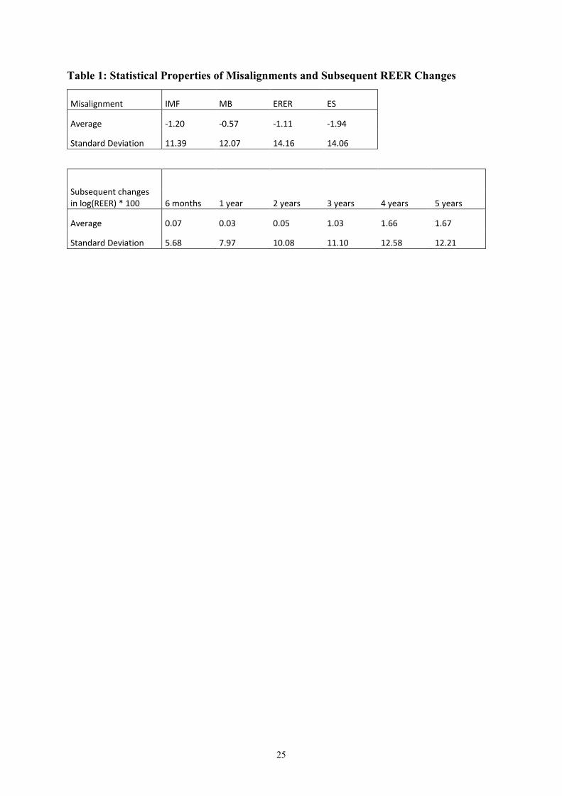
for a complete exchange rate adjustment predicted in the medium term. Table 1, in which

averages and standard deviations of the misalignment variables and the subsequent exchange

rate changes are listed, illustrates this point.

The coefficient of the linear fit is statistically different from zero in all three cases. However,

the ES Misalignment scores poorest. The coefficient of the linear fit of the ES Misalignment is

only –0.10. Furthermore, there are many outlier observations in the upper right quadrants for

the MB and ES Misalignments. In other words, there are several currencies which were

diagnosed as significantly overvalued by the MB and ES approaches but continued to appreciate

afterwards. On the other hand, the ERER Misalignment scores relatively better. There are

relatively fewer outliers in the upper right quadrant and the coefficient of the linear fit is –0.16,

implying that 16 percent of the misalignment of the exchange rate was closed within the next 2

years. Thus at a first glance, the predictive power of the ERER approach for future exchange

rate movements within the two-year horizon seems to be higher than the other two models.9

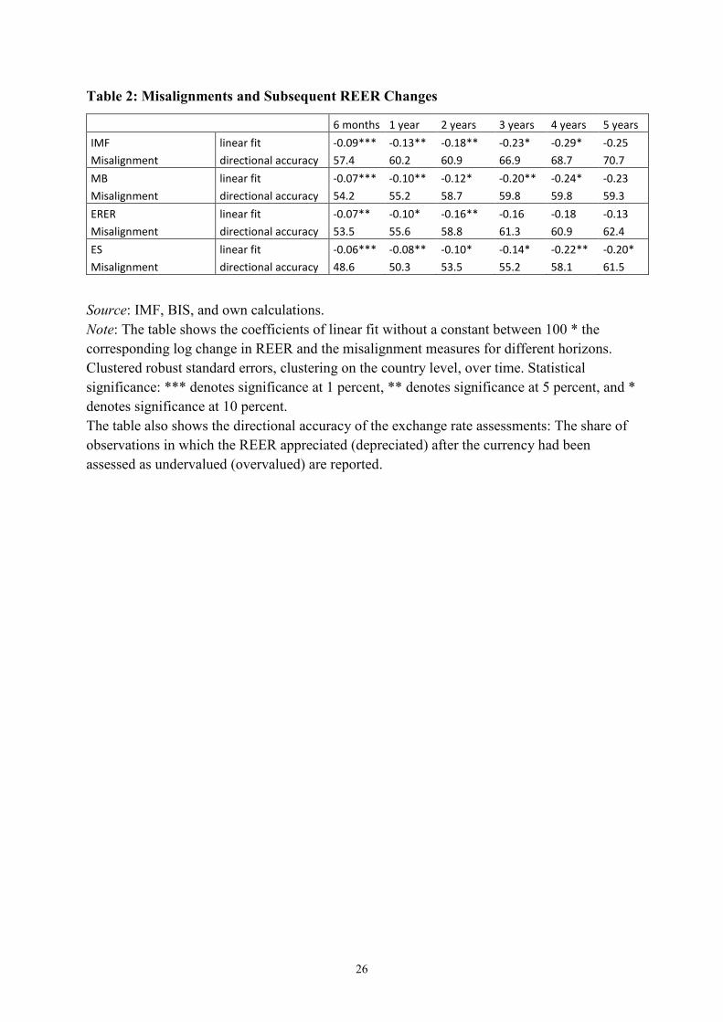
Table 2 summarizes the coefficients of linear fit and directional accuracies of the misalignment

measures for all horizons considered in the analysis. As expected, the predictive power of the

models generally increases with the length of the horizon. The linear fit coefficients for all three

9 Although the MB and ES approaches are quite different from each other methodologically, they tend to give similar assessments. The simple correlation between the MB Misalignment and ES Misalignment in the sample is 0.83. The similar assessments are, to some extent, due to these models’ implicit assumption that current account gaps are closed solely via the goods trade channel facilitated through an exchange rate adjustment. However, equilibrium current accounts are calculated completely differently.

9

9

misalignment estimates are negative and statistically significant for shorter horizons. Table 2

shows that the directional accuracy of the assessments increases with the horizon for all

misalignment variables. On the other hand, the linear fit coefficients increase only up to the 4-

year horizon. At a first glance, there are some differences between the predictive performances

of the three IMF models when country specific factors are not taken into account, particularly

when the horizon gets longer.

Are there any currencies for which the models made persistent errors in predicting the direction

of the future exchange rate movements? In other words, are there currencies which appreciated

(depreciated) more than 5 percent “too many times”, following a diagnosis either of being in

line with fundamentals or overvaluation (undervaluation) during the sample period? A closer

look at the sample reveals that there is one advanced economy currency and one emerging

market economy currency for which all three models were significantly wrong regarding the

direction of the subsequent exchange rate movement over the 2-year horizon for at least four

assessments.10

Furthermore, contrary to the bivariate regression results, the ES Misalignment makes persistent

errors (four or more times) over the 2-year horizon for the smallest number of currencies, i.e.

only two, whereas the ERER Misalignment makes a persistent error for the greatest number of

currencies, i.e. seven. The MB Misalignment, on the other hand, predicts persistently incorrectly

over the 2-year horizon for four currencies. These persistent errors in predicting the direction

of the subsequent exchange rate movements explain why, in the next subsection, there is a much

higher predictive power of assessments as well as a better fit for the data panel estimations with

fixed (currency) effects. It is also worth noting that there are two emerging market economies

where all the assessments for all three models during the sample period were spot on in terms

of direction over the 2-year horizon.

3.2. Panel estimations with fixed effects Next, panel regressions with fixed effects are carried out to control for the cross-country

differences in the sample. Table 3 shows OLS regressions of log returns in the REER two years

ahead on each of the four misalignment variables separately, namely IMF Misalignment, MB

10 For reasons of confidentiality, these currencies are not identified in the paper.

10

10

Misalignment, ERER Misalignment, and ES Misalignment. Errors are clustered at currency

level.

Table 3 supports the conjecture of the previous subsection that the IMF ‘diagnosis’ of

undervalued or overvalued currencies has some explanatory power in predicting directional

movements in the REER. All coefficients on the misalignment variables have negative signs

and are statistically significant. Furthermore, controlling for fixed effects increases the

predictive power of the assessments significantly, as mentioned in the previous subsection. This

finding confirms that assessments of REER undervaluation (overvaluation) are followed by

subsequent appreciation (depreciation) of the REER, independent of the model used for the

assessment. For example, the coefficient of the IMF Misalignment variable has the value 0.58.

That is, 58 percent of the misalignment gap is closed after 2 years when country specific factors

are taken into account. The predictive performance of the IMF assessment, however, is

explained to a large extent by the predictive performance of the ERER model. Assessments

based on the ERER model have the highest coefficient value in absolute value, together with

the highest R-square (albeit still relatively low at 0.30). According to the estimation, 59 percent

of the misalignment gap diagnosed by the ERER model is closed after two years if we control

for country effects. On the other hand, the predictive power of the MB and the ES assessments

is considerably weaker with lower R-square and lower coefficient values. This evidence

suggests that the predictive power of the IMF Misalignment is due to the high predictive power

of the ERER Misalignment.

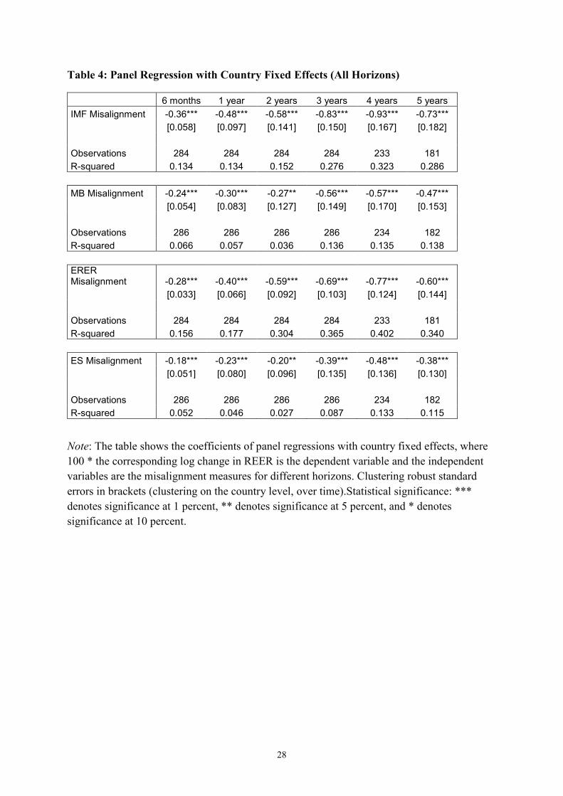
Results for the other horizons are illustrated in Table 4. Observations made for the 2-year

horizon continue to hold for the other horizons. All misalignment variables have considerable

predictive power for future exchange rate movements. All coefficients are negative and

statistically significant. However, the ERER Misalignment regression continues to have the

highest R-square values. Furthermore, it delivers the highest coefficient values in absolute value

for all horizons considered among the three misalignment variables. It is also worth noting that

the explanatory power of the misalignment variables increases, to a large extent, with the length

of the horizon until it has reached four years, and then decreases slightly over the 5-year

horizon. Based on the estimation results, 93 percent of the misalignment gap diagnosed by the

IMF is closed after four years if we control for country effects.

11

11

3.3. Controlling for the exchange rate regime There may be various reasons why the REER does not adjust fully to its calculated equilibrium

value. One argument concerns the exchange rate regime in place. If the nominal exchange rate

is not floating, it will take longer for the REER to adjust, or it will adjust only partially, if at all.

To test this possibility, the following regressions control for differences in the exchange rate

regime across countries and time. The exchange rate regime is summarized in a dummy variable

based on the IMF classification in the IMF Annual Report on Exchange Arrangements and

Exchange Restrictions (AREAER). Note that the IMF classification is based on available

information on countries’ de facto arrangements, as analyzed by IMF staff, which may differ

from countries’ officially announced (de jure) arrangements. In particular, the classification for

‘free floating’ regime is very restrictive and uses information on reserve accumulation of

countries.11

The dummy variable equals one if the exchange rate regime is classified as ‘free floating’ or

‘floating’ throughout the horizon following the exchange rate assessment. It equals zero

otherwise. 12

Furthermore, the interaction term between the exchange rate regime dummy and the

misalignment measure is included in the regressions. Additionally, a time trend is included. The

specification is the following:

log𝑅𝑅𝑅𝑅𝑅𝑅𝑅𝑅𝑅𝑅𝑅𝑅𝑅𝑅𝑅𝑅𝑗𝑗𝑗𝑗,𝑡𝑡𝑡𝑡+𝑘𝑘𝑘𝑘 − log𝑅𝑅𝑅𝑅𝑅𝑅𝑅𝑅𝑅𝑅𝑅𝑅𝑅𝑅𝑅𝑅𝑗𝑗𝑗𝑗,𝑡𝑡𝑡𝑡 = 𝛼𝛼𝛼𝛼𝑗𝑗𝑗𝑗 + 𝛽𝛽𝛽𝛽 × 𝑀𝑀𝑀𝑀𝑀𝑀𝑀𝑀𝑀𝑀𝑀𝑀𝑀𝑀𝑀𝑀𝑀𝑀𝑀𝑀𝑀𝑀𝑀𝑀𝑀𝑀𝑀𝑀𝑀𝑀𝑀𝑀𝑀𝑀𝑀𝑀𝑀𝑀𝑀𝑀𝑀𝑀𝑀𝑀𝑀𝑀𝑀𝑀𝑗𝑗𝑗𝑗,𝑡𝑡𝑡𝑡 + 𝛾𝛾𝛾𝛾 × 𝐷𝐷𝐷𝐷𝐷𝐷𝐷𝐷𝑀𝑀𝑀𝑀𝑀𝑀𝑀𝑀𝐷𝐷𝐷𝐷𝑗𝑗𝑗𝑗,𝑡𝑡𝑡𝑡→𝑡𝑡𝑡𝑡+𝑘𝑘𝑘𝑘

+𝛿𝛿𝛿𝛿 × 𝐷𝐷𝐷𝐷𝐷𝐷𝐷𝐷𝑀𝑀𝑀𝑀𝑀𝑀𝑀𝑀𝐷𝐷𝐷𝐷𝑗𝑗𝑗𝑗,𝑡𝑡𝑡𝑡→𝑡𝑡𝑡𝑡+𝑘𝑘𝑘𝑘 × 𝑀𝑀𝑀𝑀𝑀𝑀𝑀𝑀𝑀𝑀𝑀𝑀𝑀𝑀𝑀𝑀𝑀𝑀𝑀𝑀𝑀𝑀𝑀𝑀𝑀𝑀𝑀𝑀𝑀𝑀𝑀𝑀𝑀𝑀𝑀𝑀𝑀𝑀𝑀𝑀𝑀𝑀𝑀𝑀𝑀𝑀𝑀𝑀𝑗𝑗𝑗𝑗,𝑡𝑡𝑡𝑡 + 𝑇𝑇𝑇𝑇𝑀𝑀𝑀𝑀𝑀𝑀𝑀𝑀𝑀𝑀𝑀𝑀 𝑀𝑀𝑀𝑀𝑡𝑡𝑡𝑡𝑀𝑀𝑀𝑀𝑀𝑀𝑀𝑀𝑡𝑡𝑡𝑡𝑡𝑡𝑡𝑡

where j denotes the currency in question, k denotes the time horizon studied, and Dummy

denotes the exchange rate regime variable. Misalignment is either the MB, ERER, ES or IMF

Misalignment.

If the REER does not adjust fully due to a non-free-floating exchange rate regime, then the

interaction term between the dummy and the misalignment variable should be statistically

11 If information on reserve accumulation is not made available by a country, then the exchange rate regime is classified as ‘floating’ by the IMF.

12 For robustness check, a stricter definition of the exchange rate regime was used where the dummy equals 1 for only ‘free floating’ regimes. In that case, controlling for the exchange rate regime in the specification did not improve the predictability of exchange rates. The result was valid for all misalignment variables and horizons.

12

12

significant and negative. Furthermore, the fit of the model should be higher when the

exchange rate regime is taken into account.

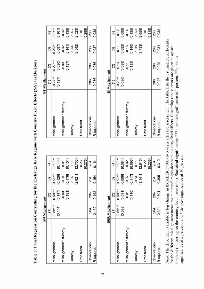
Table 5 presents the results of the panel regressions with country fixed effects using the above

specification over the two-year horizon. For robustness checks four different model

specifications are considered. Model 1 corresponds to the results shown in Table 3. Table 5

shows that none of the interaction terms is statistically significant for any misalignment

measure. Also the fit of the model does not significantly improve if the exchange rate regime

is controlled for. Thus over the two-year horizon, the exchange rate regime does not appear to

influence the predictive performance of the exchange rate assessments. Furthermore, the

coefficient of the time trend is statistically insignificant for all misalignment measures.

Next, consideration is given to the other horizons, when the exchange rate regime is

controlled for. Tables 6 and 7 illustrate the results for shorter and longer horizons,

respectively. It is worth noting that the influence of the exchange rate regime on the

adjustment depends greatly on the length of the horizon considered. In general, for the

shortest horizon, the exchange rate regime plays a relatively important role in the predictive

power of the assessments. On the other hand, for the longest horizon the exchange rate regime

is insignificant in the external adjustment process. Furthermore, the time trend remains

irrelevant in all horizons considered.

In particular, Table 6 shows that for the 6-month horizon, the interaction term is statistically

significant in all the specifications and misalignment measures considered. Furthermore, the

adjusted R-square increases in the 6-month horizon, when the exchange rate regime is

controlled for. On the other hand, for the 1-year horizon, the interaction term is not always

statistically significant. Thus the exchange rate regime plays a role in external adjustment

only in the very short run.

Table 7, on the other hand, shows that the interaction term is statistically insignificant in the

5-year horizon in all the specifications and misalignment measures considered. Controlling

for the exchange rate regime even lowers the fit of the model to the data. For the 3 and 4-year

horizons, however, the results are mixed depending on the misalignment measure used. For

example, in the 3-year horizon, controlling for the exchange rate regime increases the fit of

the model for all misalignment measures except the MB Misalignment. For the 4-year horizon,

the interaction term becomes statistically insignificant for the ERER Misalignment, and is

13

13

weakly significant for the MB Misalignment. These mixed results may be due to the specific

nature of the sample period.

Overall, it seems redundant to control for the exchange rate regime in these specifications for

longer horizons because controlling for it does not improve the fit of the model to the data in a

significant and consistent way. This might be due to the fact that exchange rate regimes do not

often change and their continuity can already be captured in country fixed effects. Thus, from

this point on, model specifications do not control for the exchange rate regime and do not

include a time trend.

Furthermore, Tables 6 and 7 confirm the previous findings that the ERER Misalignment

outperforms the MB and the ES Misalignments in terms of predicting future exchange rate

movements over all horizons and specifications considered. Thus the predictive power of the

IMF Misalignment continues to come from that of the ERER Misalignment, even when the

exchange rate regime is controlled for.

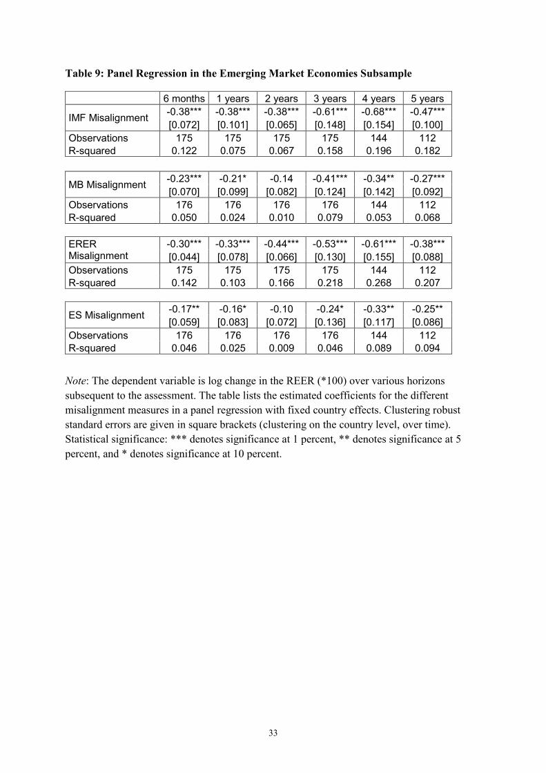
3.4. Predictive power in advanced economies versus emerging market economies

This subsection investigates the possibility that the predictive power of the misalignment

variables might differ in advanced economies (AEs) and in emerging market economies

(EMEs). Such a difference might be due to different volatilities of macroeconomic variables

and/or the availability of more detailed data for more accurate medium-term forecasts. To test

this hypothesis, the sample of countries is split into two subsamples of AEs and EMEs. Tables

8 and 9 illustrate the regression results in these subsamples. 13 A comparison of the regression

results indicate that the predictive power of the assessments for subsequent exchange rate

movements is indeed higher in AEs than in EMEs.

Confirming previous results, the ERER Misalignment outperforms the other two model-based

misalignment variables in both subsamples, both in terms of the fit of the model and in terms

of the absolute value of the coefficient. In the AEs subsample, for example, about 89 percent

of the exchange rate gap, as measured by the ERER Misalignment, is closed within 3 years of

the assessment, whereas in the EMEs subsample about 53 percent of the exchange rate gap as

measured by the ERER Misalignment is closed after 3 years. The predictive power of the MB

13 The countries and their classification are listed in Appendix B.

14

14

Misalignment and ES Misalignment is significantly better in AEs than in EMEs. In the AE

subsample, the predictive power of the IMF Misalignment is higher than the ERER

Misalignment in terms of the absolute value of the coefficient, but not in terms of the fit of the

model.

Furthermore, the absolute value of the coefficient of the misalignment variables for the AEs

subsample increases considerably in absolute value with the length of the horizon up to 4

years. For the 5-year horizon, though, the estimated coefficient is lower in absolute value.

This may be due to new macroeconomic events that are not captured in the assessments 5

years in advance. There is a similar pattern for the IMF Misalignment coefficient for the

EMEs subsample. However, for the other misalignment measures, these patterns do not

strictly hold in the EMEs subsample.

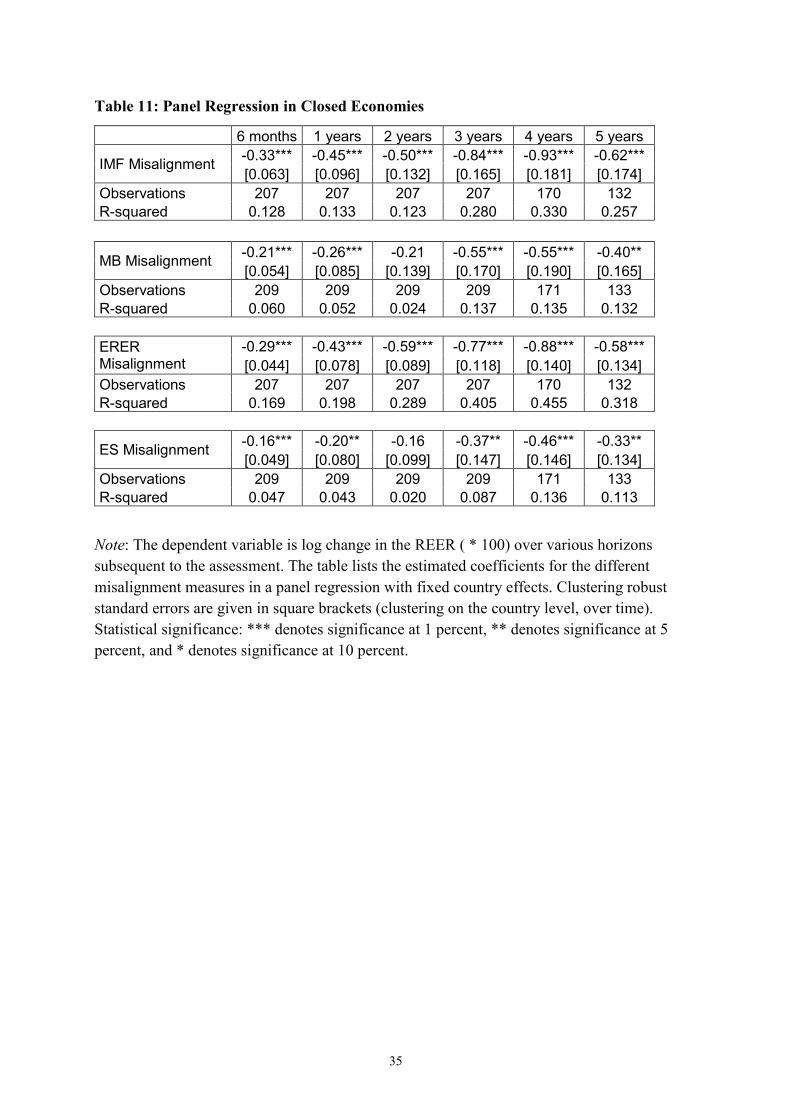
3.5. Predictive power in open versus closed economies Two of the exchange rate models, namely the MB and ES models, assume that the exchange

rate adjustment mechanism occurs through the international trade channel. In other words, the

current account gap is assumed to be closing after an exchange rate depreciation

(appreciation) through an increase (decrease) in net exports. Thus, a possible reason why

these two models’ misalignment measures may not be as powerful as the ERER model’s

misalignment measure in predicting subsequent exchange rate movements is that some

economies are not very open to international trade and it may take them much longer to

complete the external adjustment.14 To control for the differences in openness across

countries, the sample is divided into two groups. Open economies are defined as countries

where the average of exports plus imports is greater than 70 percent of GDP during the

sample period. The remaining countries are categorized as closed economies.15

Tables 10 and 11 summarize the regression results in the open and closed economy

subsamples, respectively. For all horizons considered, the fit of the MB and ES Misalignments

14 In fact, the MB and ES models account for the varying levels of openness of countries, because they use country-specific exchange rate elasticities of current accounts to calculate the necessary appreciation or depreciation of currencies to close the current account gap. Thus, the varying level of openness has an impact on the size of the exchange rate adjustment in these two models but not on its speed. By dividing the sample into open and closed economies, one can test whether open economies undergo the external adjustment much faster than closed economies.

15 The countries and their classifications are listed in Appendix B.

15

15

is found to be larger in open economies than in closed economies. However, the estimated

coefficients for open economies are not always statistically significant. This is driven by large

standard errors of the estimated coefficients. On the other hand, the estimated coefficients in

absolute value are larger in the open economies subsample compared to the closed economies

subsample. This suggests that the speed of adjustment is different in open versus closed

economies. In other words, the misalignment gap calculated in the MB and ES models

reduces generally faster and to a greater extent in open economies.

On the other hand, the predictive power of the ERER Misalignment is generally higher in the

closed economies subsample than in the open economies subsample. This may be reconciled

by the fact that the exchange rate adjustment in the ERER model does not operate through the

international trade channel.

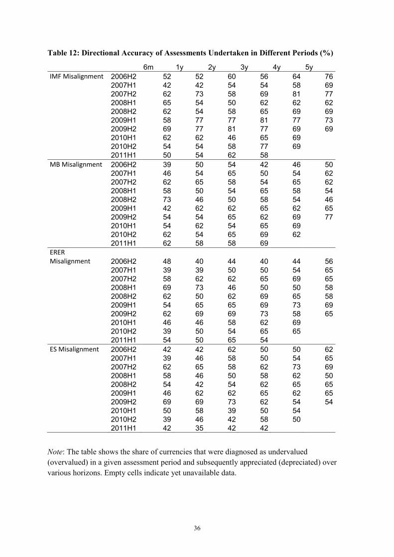
3.6. Predictive performance of different assessment vintages An interesting question concerns exchange rate adjustment during/after the financial crisis.

Were all assessment periods equally successful in predicting future exchange rate

movements? Because the sample period includes the global financial crisis, during which

significant exchange rate movements took place, assessments before the onset of the financial

crisis deserve special scrutiny. Could, for example, the exchange rate assessments made in fall

2006, spring 2007, and fall 2007 successfully predict the subsequent exchange rate

movements? How much of the exchange rate corrections that took place during the crisis were

predicted in those assessments?

Table 12 gives the directional accuracy of all assessment periods separately. In other words,

for each assessment period, it lists the share of currencies for which the misalignment gap was

reduced over various horizons. At first glance, the assessments made in fall 2006, spring

2007, and fall 2007 were not necessarily less successful than the assessments undertaken after

the onset of the crisis in predicting the direction of the subsequent REER movements. For

example, 76 percent of currencies that were diagnosed as undervalued (or overvalued) in fall

2006 according to the IMF Misalignment, had appreciated (or depreciated) by fall 2011.

Sequential bivariate regressions without fixed effects as in section 3.1 were also undertaken

for each assessment period to evaluate the predictive power of each vintage separately.

However, due to the low number of observations in each assessment period, standard errors

16

16

tend to be high and a large number of estimated coefficients prove to be statistically not

different from zero. Interestingly, however, the assessment made in fall 2007 has statistically

significant coefficients for all misalignment measures for the 4-year horizon. This finding

suggests that assessments made before the onset of the financial crisis were not necessarily

less successful in correctly predicting the exchange rate than assessments made after the

crisis. Due to space constraints and the high number of statistically insignificant findings, the

results are not shown here.

3.7. Robustness check with safe haven currencies Another interesting question concerns safe haven currencies: Are the IMF models adequate to

assess safe haven currencies because there may be other factors, such as global risk

perception, that move these currencies, especially during turbulent times? In other words, the

predictive power of the assessments may be affected by the presence of safe haven currencies

in the sample. Five currencies, namely, the US dollar, euro, British pound, Swiss franc, and

Japanese yen can be considered as safe haven currencies in the current sample according to

the previous literature; see, for example, Ranaldo and Söderlind (2010), Habib and Stracca

(2012), Grisse and Nitschka (2015), and de Bock and de Carvalho Filho (2015), among

others.

In order to check the robustness of the previous findings, panel analysis with country fixed

effects are undertaken in three additional subsamples which include/exclude safe haven

currencies. The first sample includes all currencies in the original sample; these results

correspond to the results shown in Table 4 in section 3.2. The second sample includes all

currencies except the US dollar. The third sample includes all currencies except the five safe

haven currencies mentioned above. And finally, the fourth sample consists only of these five

safe haven currencies.

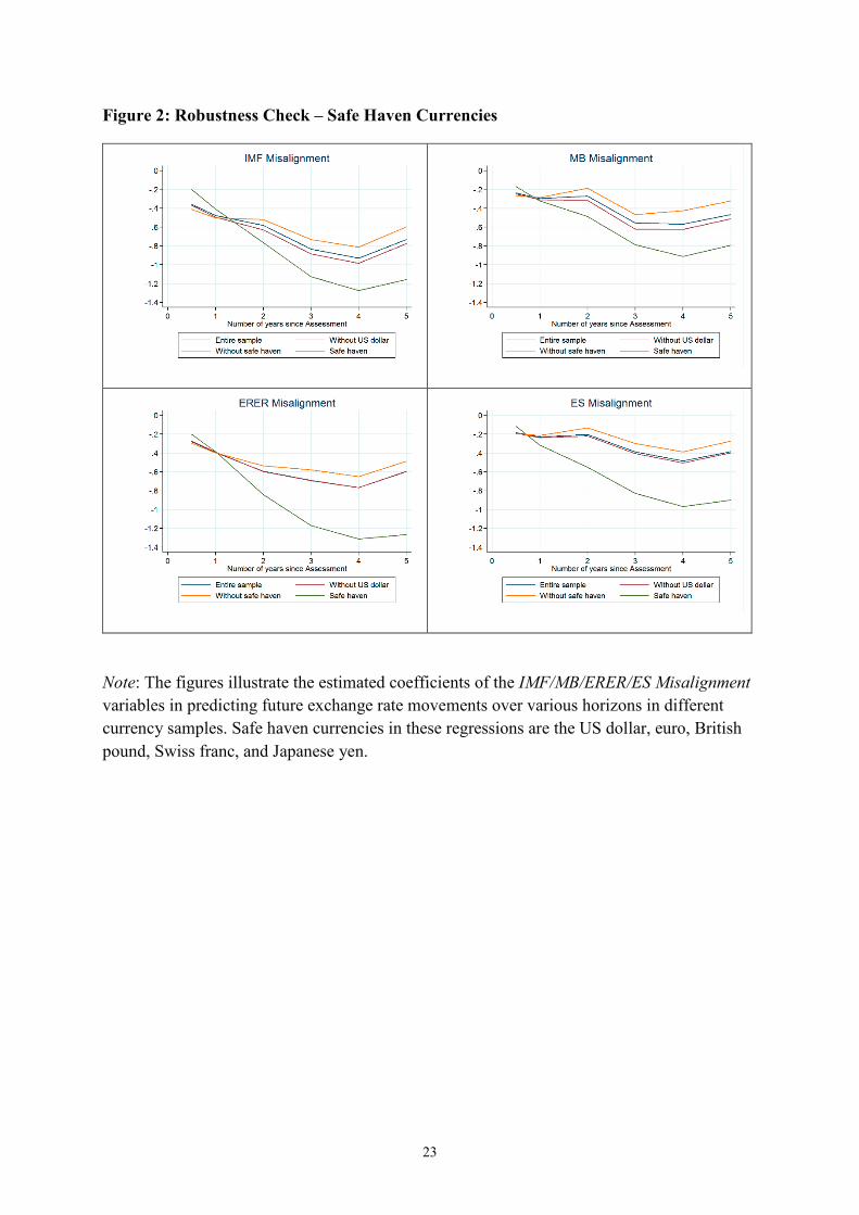
Figure 2 graphically illustrates the estimated coefficients of the misalignment variables over

various horizons. All estimated coefficients in all samples are negative. The majority of them

are also statistically significant.16 A few striking observations can be made regarding Figure

2. First, the misalignment gaps of safe haven currencies close faster, in relative terms, than do

16 A table with the estimated coefficients and standard errors is not shown due to space constraints. All coefficients are significant for the ERER Misalignment. Some of the coefficients are insignificant for the safe haven subsample for the other Misalignment variables due to a large standard error.

17

17

those of the remaining currencies. This observation is valid for all misalignment variables and

over all horizons considered, except the 6-month horizon. Thus, over the very short horizon,

the IMF models do not have much predictive power for safe haven currencies, whereas they

have significantly higher predictive power over longer horizons. For example, three years

after the assessment, the IMF misalignment gap is completely closed in the safe haven

subsample (the coefficient estimate is 1). Second, excluding safe haven currencies from the

sample yields lower estimated coefficients in absolute value in general but does not

significantly change the results laid out in the previous subsections.

Figure 2 also confirms the previous finding that over the 5-year horizon the estimated

coefficients are lower in absolute value than the coefficients over the 4-year horizon. This

result may be driven by significant changes in the outlook for underlying exchange rate

fundamentals, such that the assessments no longer reflect the current situation. Alternatively,

at the 5-year horizon the benefits of allowing the exchange rate longer time to adjust are lower

than the cost of changing macroeconomic determinants.

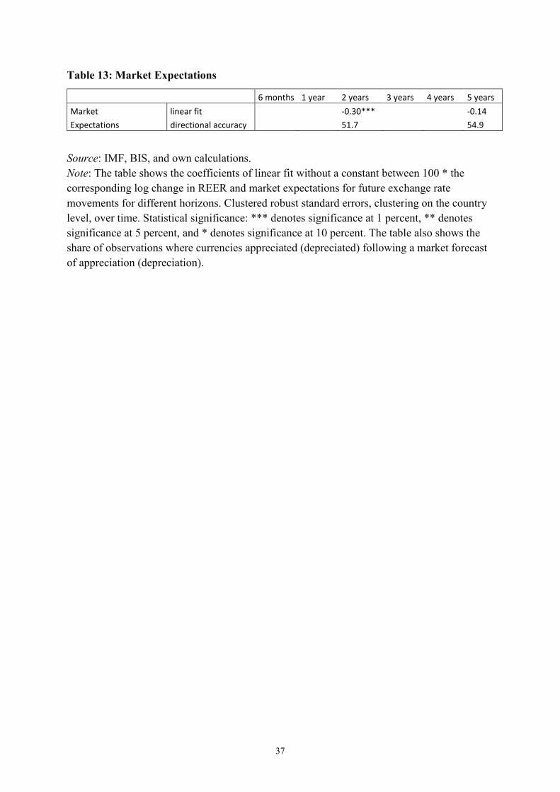
3.8. Predictive power of market expectations Can market analysts’ forecasts predict future exchange rate movements better than the IMF’s

state-of-the-art models? The documents where the IMF assessments were taken from, namely

the IMF Office Memorandums on the Exchange Rate Assessments for Selected Advanced and

Emerging Market Economies, also report on market expectations of changes in REER. These

market expectations are calculated by the IMF based on information obtained from Consensus

Forecasts. They are weighted averages of bilateral real exchange rate forecasts vis-à-vis the US

dollar where nominal exchange rate expectations and inflation projections are taken from

Consensus Forecasts (or the WEO database when unavailable).

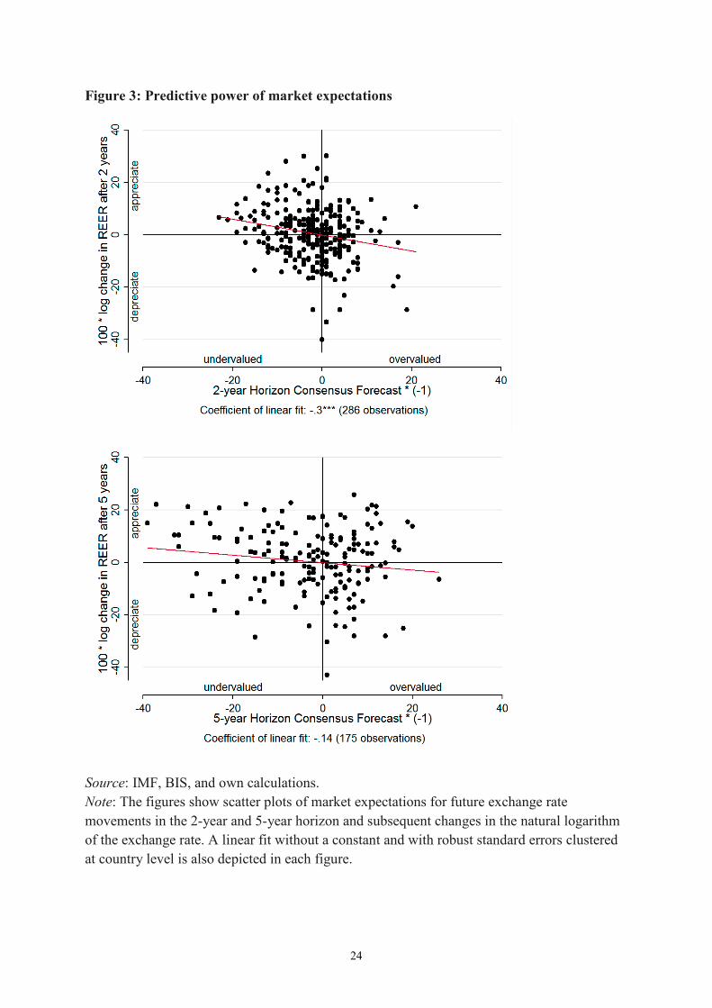
Figure 3 illustrates scatter plots of market expectations and subsequent REER movements in

the 2- and 5-year horizons. Overall, in the 2-year horizon, market expectations seem to be a

good predictor of exchange rate movements. A comparison with Figure 1 confirms that there

are less outliers in the first and third quadrants in Figure 3. Furthermore, the linear fit has a

statistically significant coefficient. In fact, on average 30 percent of the market expected

exchange rate movement takes place after two years when country specific factors are not taken

into account. The predictive power of market expectations declines with the length of the

18

18

horizon. The bottom panel of Figure 3 shows that there are more outliers in the upper right and

bottom left quadrants so that the coefficient of the linear fit becomes statistically insignificant

for the 5-year horizon.

Table 13 lists the coefficients of the linear fit as well as the directional accuracy of market

expectations. A comparison with Tables 2 leads to the conjecture that the directional accuracy

of the IMF assessments is higher than market expectations both in the 2 and 5-year horizons.

4. Conclusion This paper has tested whether the IMF’s exchange rate assessments have predictive content for

future exchange rate movements. The analysis has revealed that the IMF ‘diagnosis’ of

undervalued or overvalued currencies based on state-of-the-art models is predictive of future

exchange rate movements.

Interestingly, one of the models, namely the ERER model, outperforms not only the other two

in predicting future exchange rate movements, but also the (average) IMF assessment.

Furthermore, the IMF assessments are better at predicting future exchange rate movements in

advanced economies than in emerging market economies. Controlling for the exchange rate

regime does not yield different results. Furthermore, the IMF assessments have higher

predictive performance in open economies than in closed economies. Last but not least, safe

haven currencies close the misalignment gap predicted by the models faster than other

currencies.

The analysis has certain limitations. First of all, the sample period is rather short. The IMF

conducted the CGER analysis between 2006 and 2011. This limits the number of observations

that can be tested for the exchange rate adjustment over the longer horizon. Second, the period

includes the global financial crisis and the euro area sovereign debt crisis. Such turbulent times

were not foreseen by the IMF or any other institution ex ante, and certainly were not taken into

account in the exchange rate assessments previously. Nevertheless, assessments made until the

onset of the financial crisis do not exhibit less accuracy in predicting the direction of the future

exchange rate movements. Last but not least, the analysis does not control for subsequent

revisions to the IMF outlook for macroeconomic variables. This is done intentionally, as the

aim of the paper is to test how well the exchange rate assessments made by the state-of-the-art

models can predict future exchange rate movements ex-ante. In fact, the whole exercise is a

19

19

joint test of the IMF exchange rate models and macroeconomic outlooks for exchange rate

predictability.

The findings suggest that the ERER model predicts future exchange rate movements on average

better than the other two models. Nevertheless, there are still significant gains from using the

other two exchange rate models to assess exchange rates. First of all, no single model is good

for all currencies. In fact, the ERER model can also make persistent errors for certain currencies,

whereas the MB and the ES models perform better in that respect. Furthermore, the ERER

model is only a reduced form model, whereas the MB and ES models are based on some

theoretical considerations. In the context of the global imbalances debate, the MB and ES

models are therefore more attractive from an international institution’s perspective to utilize,

even if they are not as successful to predict future exchange rate movements. Recently,

however, the IMF changed its external sector assessment framework. To assess exchange rates

only a modified version of the ERER model is being used since 2012. The modified versions

of the MB and ES models, while still being utilized, do not have a direct link to the exchange

rate anymore. That is, the IMF ceased making a direct link from equilibrium current accounts

to equilibrium exchange rates for now.

20

20

5. References Abiad, Abdul, Prakash Kannan, and Jungjin Lee (2009), “Evaluating Historical CGER

Assessments: How Well Have They Predicted Subsequent Exchange Rate Movements?”, IMF

Working Paper, No. 09/32.

Beusch, Elisabeth, Barbara Döbeli, Andreas M. Fischer, and Pınar Yeşin (2014), “Merchanting

and Current Account Balances”, CEPR Discussion Paper, No 9990.

Bussière, Matthieu, Michele Ca’ Zorzi, Alexander Chudík, and Alistair Dieppe,

“Methodological Advances in the Assessment of Equilibrium Exchange Rates”, ECB Working

Paper Series, No 1151.

Chinn, Menzie D. and Eswar Prasad (2003), “Medium-term Determinants of Current Accounts

in Industrial and Developing Countries: an Empirical Exploration”, Journal of International

Economics, No. 59, pages 47–76.

de Bock, Reinout and Irineu de Carvalho Filho (2015), “The Behavior of Currencies during

Risk-off Episodes”, Journal of International Money and Finance, No. 53, pages 218–234.

Evans, Martin D. D. and Richard K. Lyons (2006), “Understanding order flow”, International

Journal of Finance and Economics, Vol. 11, No. 1, pages 3–23.

Fischer, Andreas M., Jessica Leutert, and Pınar Yeşin (2012), “Persistent Surpluses: Modeling

the Swiss Current Account Using the Absorption Approach”, unpublished manuscript, Swiss

National Bank, March 2012.

Grisse, Christian and Thomas Nitschka (2015), “On Financial Risk and the Safe Haven

Characteristics of Swiss Franc Exchange Rates”, Journal of Empirical Finance, Vol. 32, pages

153–164.

Habib, Maurizio M. and Livio Stracca (2012), “Getting beyond carry trade: What makes a safe

haven currency?”, Journal of International Economics, Vol. 87, pages 50–64.

Isard, Peter and Hamid Faruqee (1998), “Exchange Rate Assessment: Extensions of the

Macroeconomic Balance Approach”, IMF Occasional Paper, No. 167.

Isard, Peter, Hamid Faruqee, G. Russell Kincaid, and Martin Fetherston (2001), “Methodology

for Current Account and Exchange Rate Assessments”, IMF Occasional Paper, No. 209.

21

21

Lee, Jaewoo, Gian Maria Milesi-Ferretti, Jonathan Ostry, Alessandro Prati, and Luca Antonio

Ricci (2008), “Exchange Rate Assessments: CGER Methodologies”, IMF Occasional Paper,

No. 261.

Meese, Richard A. and Kenneth Rogoff (1983a), “Empirical Exchange Rate Models of the

Seventies: Do they fit out of sample?”, Journal of International Economics, Vol. 14, pages 3–

24.

Meese, Richard A. and Kenneth Rogoff (1983b), “The out-of sample failure of empirical

exchange rates: sampling error or misspecification?”, in J. Frenkel (ed.) Exchange Rates and

International Macroeconomics, pp. 67–105, Chicago: NBER and University of Chicago Press.

Phillips, Steven, Luis Catão, Luca Ricci, Rudolfs Bems, Mitali Das, Julian Di Giovanni, D.

Filiz Unsal, Marola Castillo, Jungjin Lee, Jair Rodriguez, and Mauricio Vargas (2013), “The

External Balance Assessment (EBA) Methodology”, IMF Working Paper, No. 13/272.

Ranaldo, Angelo and Paul Söderlind (2010), “Safe Haven Currencies”, Review of Finance, Vol.

14, pages 385–407.

22

22

6. Figures and Tables

Figure 1: Misalignments and Two-year Ahead REER Changes

Source: IMF, BIS, and own calculations. Note: The figures show scatter plots of the different misalignment measures and the two-year-ahead changes in the natural logarithm of the REER following the assessments. A linear fit without a constant and with robust standard errors clustered at country level is also depicted in each figure.

23

23

Figure 2: Robustness Check – Safe Haven Currencies

Note: The figures illustrate the estimated coefficients of the IMF/MB/ERER/ES Misalignment variables in predicting future exchange rate movements over various horizons in different currency samples. Safe haven currencies in these regressions are the US dollar, euro, British pound, Swiss franc, and Japanese yen.

24

24

Figure 3: Predictive power of market expectations

Source: IMF, BIS, and own calculations. Note: The figures show scatter plots of market expectations for future exchange rate movements in the 2-year and 5-year horizon and subsequent changes in the natural logarithm of the exchange rate. A linear fit without a constant and with robust standard errors clustered at country level is also depicted in each figure.

25

25

Table 1: Statistical Properties of Misalignments and Subsequent REER Changes

Misalignment IMF MB ERER ES

Average -1.20 -0.57 -1.11 -1.94

Standard Deviation 11.39 12.07 14.16 14.06

Subsequent changes in log(REER) * 100

6 months 1 year 2 years 3 years 4 years 5 years

Average 0.07 0.03 0.05 1.03 1.66 1.67

Standard Deviation 5.68 7.97 10.08 11.10 12.58 12.21

26

26

Table 2: Misalignments and Subsequent REER Changes

6 months 1 year 2 years 3 years 4 years 5 years IMF linear fit -0.09*** -0.13** -0.18** -0.23* -0.29* -0.25 Misalignment directional accuracy 57.4 60.2 60.9 66.9 68.7 70.7 MB linear fit -0.07*** -0.10** -0.12* -0.20** -0.24* -0.23 Misalignment directional accuracy 54.2 55.2 58.7 59.8 59.8 59.3 ERER linear fit -0.07** -0.10* -0.16** -0.16 -0.18 -0.13 Misalignment directional accuracy 53.5 55.6 58.8 61.3 60.9 62.4 ES linear fit -0.06*** -0.08** -0.10* -0.14* -0.22** -0.20* Misalignment directional accuracy 48.6 50.3 53.5 55.2 58.1 61.5

Source: IMF, BIS, and own calculations. Note: The table shows the coefficients of linear fit without a constant between 100 * the corresponding log change in REER and the misalignment measures for different horizons. Clustered robust standard errors, clustering on the country level, over time. Statistical significance: *** denotes significance at 1 percent, ** denotes significance at 5 percent, and * denotes significance at 10 percent. The table also shows the directional accuracy of the exchange rate assessments: The share of observations in which the REER appreciated (depreciated) after the currency had been assessed as undervalued (overvalued) are reported.

27

27

Table 3: Panel Regression with Country Fixed Effects (2-Years Horizon)

IMF MB ERER ES Coefficient of the misalignment assessment

-0.58*** -0.27** -0.59*** -0.20** [0.141] [0.127] [0.092] [0.096]

Observations 284 286 284 286 R-squared 0.152 0.036 0.304 0.027

Note: The table shows the coefficients of linear fit without a constant between 100 * the log change in REER until two years after the assessment and and the misalignment measures. Clustering robust standard errors in brackets (clustering on the country level, over time). Statistical significance: *** denotes significance at 1 percent, ** denotes significance at 5 percent, and * denotes significance at 10 percent.

28

28

Table 4: Panel Regression with Country Fixed Effects (All Horizons)

6 months 1 year 2 years 3 years 4 years 5 years IMF Misalignment -0.36*** -0.48*** -0.58*** -0.83*** -0.93*** -0.73*** [0.058] [0.097] [0.141] [0.150] [0.167] [0.182] Observations 284 284 284 284 233 181 R-squared 0.134 0.134 0.152 0.276 0.323 0.286 MB Misalignment -0.24*** -0.30*** -0.27** -0.56*** -0.57*** -0.47*** [0.054] [0.083] [0.127] [0.149] [0.170] [0.153] Observations 286 286 286 286 234 182 R-squared 0.066 0.057 0.036 0.136 0.135 0.138 ERER Misalignment -0.28*** -0.40*** -0.59*** -0.69*** -0.77*** -0.60*** [0.033] [0.066] [0.092] [0.103] [0.124] [0.144] Observations 284 284 284 284 233 181 R-squared 0.156 0.177 0.304 0.365 0.402 0.340 ES Misalignment -0.18*** -0.23*** -0.20** -0.39*** -0.48*** -0.38*** [0.051] [0.080] [0.096] [0.135] [0.136] [0.130] Observations 286 286 286 286 234 182 R-squared 0.052 0.046 0.027 0.087 0.133 0.115

Note: The table shows the coefficients of panel regressions with country fixed effects, where 100 * the corresponding log change in REER is the dependent variable and the independent variables are the misalignment measures for different horizons. Clustering robust standard errors in brackets (clustering on the country level, over time).Statistical significance: *** denotes significance at 1 percent, ** denotes significance at 5 percent, and * denotes significance at 10 percent.

29

29

Tab

le 5

: Pan

el R

egre

ssio

n C

ontr

ollin

g fo

r th

e E

xcha

nge

Rat

e R

egim

e w

ith C

ount

ry F

ixed

Eff

ects

(2-Y

ears

Hor

izon

)

IMF

Mis

alig

nmen

t

MB

Mis

alig

nmen

t

(1)

(2)

(3)

(4)

(1)

(2)

(3)

(4)

Mis

alig

nmen

t -0

.58*

**

-0.5

8***

-0

.55*

**

-0.6

2***

Mis

alig

nmen

t -0

.27*

* -0

.27*

**

-0.2

6***

-0

.27*

*

[0.1

41]

[0.1

47]

[0.1

29]

[0.1

44]

[0.1

27]

[0.0

90]

[0.0

87]

[0.1

01]

Mis

alig

nmen

t * d

umm

y

-0.0

0 -0

.04

0.01

Mis

alig

nmen

t * d

umm

y

-0.0

0 -0

.02

-0.0

2

[0

.181

] [0

.178

] [0

.151

]

[0.1

37]

[0.1

41]

[0.1

38]

Dum

my

-1.9

2 -1

.09

D

umm

y

-1

.64

-1.4

3

[2.9

21]

[2.7

33]

[2.5

42]

[2.5

23]

Tim

e tre

nd

0.

26

Ti

me

trend

0.10

[0

.276

]

[0.2

99]

Obs

erva

tions

28

4 28

4 28

4 28

4

Obs

erva

tions

28

6 28

6 28

6 28

6 R

-squ

ared

0.

152

0.15

2 0.

154

0.16

1

R-s

quar

ed

0.03

6 0.

036

0.03

7 0.

038

ERER

Mis

alig

nmen

t

ES M

isal

ignm

ent

(1

) (2

) (3

) (4

)

(1

) (2

) (3

) (4

) M

isal

ignm

ent

-0.5

9***

-0

.58*

**

-0.5

8***

-0

.62*

**

M

isal

ignm

ent

-0.2

0**

-0.1

3 -0

.11

-0.1

2

[0.0

92]

[0.0

91]

[0.0

89]

[0.0

84]

[0.0

96]

[0.0

88]

[0.0

82]

[0.0

99]

Mis

alig

nmen

t * d

umm

y

-0.0

1 -0

.02

0.02

Mis

alig

nmen

t * d

umm

y

-0.1

1 -0

.15

-0.1

4

[0

.110

] [0

.117

] [0

.097

]

[0.1

33]

[0.1

40]

[0.1

35]

Dum

my

-0.5

4 0.

11

D

umm

y

-1

.98

-1.6

9

[3.1

41]

[2.9

15]

[2.7

33]

[2.6

59]

Tim

e tre

nd

0.

22

Ti

me

trend

0.10

[0

.236

]

[0.3

15]

Obs

erva

tions

28

4 28

4 28

4 28

4

Obs

erva

tions

28

6 28

6 28

6 28

6 R

-squ

ared

0.

304

0.30

4 0.

305

0.31

0

R-s

quar

ed

0.02

7 0.

029

0.03

1 0.

032

Not

e: T

he d

epen

dent

var

iabl

e is

log

chan

ge in

the

REE

R (*

100)

two

year

s afte

r the

ass

essm

ent.

The

tabl

e lis

ts th

e es

timat

ed c

oeff

icie

nts

for t

he d

iffer

ent m

isal

ignm

ent m

easu

res i

n a

pane

l reg

ress

ion

with

cou

ntry

fixe

d ef

fect

s. C

lust

erin

g ro

bust

err

ors a

re g

iven

in sq

uare

br

acke

ts (c

lust

erin

g on

the

coun

try le

vel,

over

tim

e). S

tatis

tical

sign

ifica

nce:

***

den

otes

sign

ifica

nce

at 1

per

cent

, **

deno

tes

sign

ifica

nce

at 5

per

cent

, and

* d

enot

es si

gnifi

canc

e at

10

perc

ent.

30

30

Table 6: Exchange Rate Regime and External Adjustment over Shorter Horizons

Note: The dependent variable is percentage change in the REER 6 months and 1 year after the assessment, respectively. The table lists the estimated coefficients for the different misalignment measures in a panel regression with fixed country effects. Robust standard errors clustered at currency level are given in square brackets. Statistical significance: *** denotes significance at 1 percent, ** denotes significance at 5 percent, and * denotes significance at 10 percent.

Model 1 Model 2 Model 3 Model 4 Model 1 Model 2 Model 3 Model 4IMF Misalignment -0.36*** -0.20** -0.14** -0.16** -0.48*** -0.44*** -0.30*** -0.32***

[0.058] [0.080] [0.064] [0.067] [0.097] [0.104] [0.084] [0.094]IMF Misalignment * Dummy -0.20** -0.27*** -0.26*** -0.04 -0.22** -0.21**

[0.094] [0.083] [0.083] [0.104] [0.103] [0.100]Dummy -3.24*** -3.41*** -5.70*** -5.40***

[1.091] [1.114] [1.329] [1.401]Time trend 0.11 0.11

[0.108] [0.161]Observations 284 284 284 284 284 284 284 284R-squared 0.134 0.146 0.161 0.164 0.134 0.135 0.150 0.152

MB Misalignment -0.24*** -0.09** -0.06 -0.07 -0.30*** -0.29*** -0.23*** -0.23***[0.054] [0.040] [0.041] [0.047] [0.083] [0.078] [0.051] [0.057]

MB Misalignment * Dummy -0.18*** -0.23*** -0.23*** -0.00 -0.10 -0.10[0.064] [0.067] [0.068] [0.088] [0.067] [0.067]

Dummy -2.99** -3.15** -4.93*** -4.85***[1.378] [1.422] [1.400] [1.406]

Time trend 0.08 0.06[0.081] [0.148]

Observations 286 286 286 286 286 286 286 286R-squared 0.066 0.076 0.089 0.091 0.057 0.057 0.071 0.072

ERER Misalignment -0.28*** -0.16*** -0.14*** -0.15*** -0.40*** -0.34*** -0.26*** -0.27***[0.033] [0.046] [0.040] [0.042] [0.066] [0.039] [0.039] [0.046]

ERER Misalignment * Dummy -0.15** -0.17*** -0.17*** -0.07 -0.15*** -0.15**[0.055] [0.053] [0.055] [0.050] [0.055] [0.055]

Dummy -2.35** -2.44** -3.67*** -3.52***[0.968] [0.930] [0.787] [0.909]

Time trend 0.05 0.05[0.114] [0.168]


ES Misalignment -0.18*** -0.07* -0.03 -0.04 -0.23*** -0.14 -0.05 -0.05[0.051] [0.038] [0.026] [0.030] [0.080] [0.102] [0.072] [0.078]

ES Misalignment * Dummy -0.18*** -0.25*** -0.24*** -0.12 -0.29*** -0.28***[0.061] [0.063] [0.062] [0.108] [0.100] [0.096]

Dummy -3.59*** -3.74*** -6.98*** -6.86***[1.079] [1.119] [1.489] [1.403]

Time trend 0.09 0.06[0.088] [0.156]


6 months 1 year

31

31

Table 7: Exchange Rate Regime and External Adjustment over Longer Horizons

Note: The dependent variable is percentage change in the REER 6 months and 1 year after the assessment, respectively. The table lists the estimated coefficients for the different misalignment measures in a panel regression with fixed country effects. Standard errors are given in square brackets. Statistical significance: *** denotes significance at 1 percent, ** denotes significance at 5 percent, and * denotes significance at 10 percent.

Model 1 Model 2 Model 3 Model 4 Model 1 Model 2 Model 3 Model 4 Model 1 Model 2 Model 3 Model 4IMF Misalignment -0.83*** -0.09 -0.10 -0.00 -0.93*** -0.22* -0.20** -0.17 -0.73*** -0.35** -0.36** -0.34

[0.150] [0.080] [0.075] [0.125] [0.167] [0.110] [0.093] [0.129] [0.182] [0.140] [0.143] [0.224]IMF Misalignment * Dummy -0.72*** -0.72*** -0.82*** -0.65*** -0.67*** -0.70*** -0.11 -0.12 -0.13

[0.165] [0.165] [0.165] [0.202] [0.192] [0.198] [0.203] [0.204] [0.231]Dummy 0.73 0.30 -1.90 -1.95 3.17 3.23

[3.263] [3.336] [4.480] [4.277] [5.893] [5.935]Time trend -0.31 -0.13 -0.09

[0.361] [0.471] [0.800]Observations 284 235 235 235 233 183 183 183 181 131 131 131R-squared 0.276 0.281 0.281 0.289 0.323 0.317 0.319 0.319 0.286 0.148 0.155 0.156

MB Misalignment -0.56*** -0.07 -0.08 -0.05 -0.57*** -0.17 -0.17* -0.17 -0.47*** -0.27** -0.26* -0.22[0.149] [0.066] [0.063] [0.087] [0.170] [0.101] [0.094] [0.105] [0.153] [0.121] [0.135] [0.157]

MB Misalignment * Dummy -0.43** -0.42** -0.44** -0.38* -0.39* -0.38* 0.04 0.02 0.01[0.161] [0.162] [0.164] [0.190] [0.188] [0.192] [0.156] [0.178] [0.190]

Dummy 0.33 0.17 -3.70 -3.73 1.06 1.62[2.354] [2.380] [3.676] [3.858] [6.014] [5.779]

Time trend -0.23 0.10 -0.41[0.402] [0.526] [0.663]

Observations 286 236 236 236 234 184 184 184 182 132 132 132R-squared 0.136 0.121 0.121 0.125 0.135 0.152 0.157 0.157 0.138 0.062 0.063 0.071

ERER Misalignment -0.69*** -0.30*** -0.30*** -0.21** -0.77*** -0.33* -0.35* -0.27 -0.60*** -0.24* -0.32 -0.25[0.103] [0.105] [0.095] [0.094] [0.124] [0.168] [0.192] [0.183] [0.144] [0.135] [0.204] [0.219]

ERER Misalignment * Dummy -0.40** -0.40** -0.51*** -0.36 -0.34 -0.47* -0.21 -0.17 -0.25[0.169] [0.152] [0.124] [0.224] [0.246] [0.232] [0.299] [0.296] [0.279]

Dummy 4.47 4.17 2.34 2.28 7.28 7.31[3.127] [3.276] [5.272] [4.776] [7.749] [7.385]

Time trend -0.46 -0.65 -0.52[0.308] [0.436] [0.699]


ES Misalignment -0.39*** 0.06 0.06 0.10 -0.48*** -0.00 0.01 0.01 -0.38*** -0.17* -0.16 -0.13[0.135] [0.062] [0.055] [0.085] [0.136] [0.080] [0.066] [0.089] [0.130] [0.099] [0.099] [0.129]

ES Misalignment * Dummy -0.53*** -0.53*** -0.57*** -0.55*** -0.57*** -0.56*** -0.09 -0.10 -0.11[0.130] [0.128] [0.134] [0.150] [0.143] [0.153] [0.149] [0.151] [0.166]

Dummy -0.36 -0.70 -3.08 -3.07 2.39 2.68[3.300] [3.522] [3.837] [3.862] [5.731] [5.607]

Time trend -0.28 0.02 -0.30[0.424] [0.543] [0.701]


3 years 4 years 5 years

32

Table 8: Panel Regression in the Advanced Economies Subsample

6 months 1 year 2 years 3 years 4 years 5 years

IMF Misalignment -0.33*** -0.61*** -0.86** -1.14*** -1.27*** -1.07** [0.100] [0.176] [0.285] [0.265] [0.299] [0.355]

Observations 109 109 109 109 89 69 R-squared 0.163 0.266 0.308 0.466 0.525 0.418

MB Misalignment -0.25** -0.41** -0.45 -0.75** -0.83** -0.67* [0.089] [0.150] [0.285] [0.325] [0.351] [0.314]

Observations 110 110 110 110 90 70 R-squared 0.102 0.138 0.092 0.228 0.277 0.216 ERER Misalignment

-0.25*** -0.48*** -0.78*** -0.89*** -0.95*** -0.83*** [0.050] [0.097] [0.121] [0.142] [0.176] [0.214]


ES Misalignment -0.22* -0.41** -0.46 -0.76** -0.88** -0.70* [0.101] [0.162] [0.286] [0.303] [0.345] [0.359]


Note: The dependent variable is log change in the REER (*100) over various horizons subsequent to the assessment. The table lists the estimated coefficients for the different misalignment measures in a panel regression with fixed country effects. Clustering robust standard errors are given in square brackets (clustering on the country level, over time). Statistical significance: *** denotes significance at 1 percent, ** denotes significance at 5 percent, and * denotes significance at 10 percent.

33

33

Table 9: Panel Regression in the Emerging Market Economies Subsample

6 months 1 years 2 years 3 years 4 years 5 years

IMF Misalignment -0.38*** -0.38*** -0.38*** -0.61*** -0.68*** -0.47*** [0.072] [0.101] [0.065] [0.148] [0.154] [0.100]


MB Misalignment -0.23*** -0.21* -0.14 -0.41*** -0.34** -0.27*** [0.070] [0.099] [0.082] [0.124] [0.142] [0.092]


-0.30*** -0.33*** -0.44*** -0.53*** -0.61*** -0.38*** [0.044] [0.078] [0.066] [0.130] [0.155] [0.088]


ES Misalignment -0.17** -0.16* -0.10 -0.24* -0.33** -0.25** [0.059] [0.083] [0.072] [0.136] [0.117] [0.086]



34

34

Table 10: Panel Regression in Open Economies


IMF Misalignment -0.46*** -0.59* -0.95* -0.82* -0.91 -1.18** [0.098] [0.296] [0.420] [0.401] [0.473] [0.473]


MB Misalignment -0.39* -0.47 -0.65* -0.62* -0.69 -0.86* [0.188] [0.276] [0.274] [0.300] [0.392] [0.380]


-0.24*** -0.32 -0.60* -0.48 -0.51 -0.62 [0.044] [0.165] [0.249] [0.247] [0.304] [0.333]


ES Misalignment -0.38* -0.45 -0.55 -0.52 -0.66 -0.86** [0.191] [0.290] [0.307] [0.314] [0.348] [0.339]



35

35

Table 11: Panel Regression in Closed Economies


IMF Misalignment -0.33*** -0.45*** -0.50*** -0.84*** -0.93*** -0.62*** [0.063] [0.096] [0.132] [0.165] [0.181] [0.174]


MB Misalignment -0.21*** -0.26*** -0.21 -0.55*** -0.55*** -0.40** [0.054] [0.085] [0.139] [0.170] [0.190] [0.165]


-0.29*** -0.43*** -0.59*** -0.77*** -0.88*** -0.58*** [0.044] [0.078] [0.089] [0.118] [0.140] [0.134]


ES Misalignment -0.16*** -0.20** -0.16 -0.37** -0.46*** -0.33** [0.049] [0.080] [0.099] [0.147] [0.146] [0.134]


Note: The dependent variable is log change in the REER ( * 100) over various horizons subsequent to the assessment. The table lists the estimated coefficients for the different misalignment measures in a panel regression with fixed country effects. Clustering robust standard errors are given in square brackets (clustering on the country level, over time). Statistical significance: *** denotes significance at 1 percent, ** denotes significance at 5 percent, and * denotes significance at 10 percent.

36

36

Table 12: Directional Accuracy of Assessments Undertaken in Different Periods (%)

6m 1y 2y 3y 4y 5y IMF Misalignment 2006H2 52 52 60 56 64 76 2007H1 42 42 54 54 58 69 2007H2 62 73 58 69 81 77 2008H1 65 54 50 62 62 62 2008H2 62 54 58 65 69 69 2009H1 58 77 77 81 77 73 2009H2 69 77 81 77 69 69 2010H1 62 62 46 65 69 2010H2 54 54 58 77 69 2011H1 50 54 62 58 MB Misalignment 2006H2 39 50 54 42 46 50 2007H1 46 54 65 50 54 62 2007H2 62 65 58 54 65 62 2008H1 58 50 54 65 58 54 2008H2 73 46 50 58 54 46 2009H1 42 62 62 65 62 65 2009H2 54 54 65 62 69 77 2010H1 54 62 54 65 69 2010H2 62 54 65 69 62 2011H1 62 58 58 69 ERER Misalignment 2006H2 48 40 44 40 44 56 2007H1 39 39 50 50 54 65 2007H2 58 62 62 65 69 65 2008H1 69 73 46 50 50 58 2008H2 62 50 62 69 65 58 2009H1 54 65 65 69 73 69 2009H2 62 69 69 73 58 65 2010H1 46 46 58 62 69 2010H2 39 50 54 65 65 2011H1 54 50 65 54 ES Misalignment 2006H2 42 42 62 50 50 62 2007H1 39 46 58 50 54 65 2007H2 62 65 58 62 73 69 2008H1 58 46 50 58 62 50 2008H2 54 42 54 62 65 65 2009H1 46 62 62 65 62 65 2009H2 69 69 73 62 54 54 2010H1 50 58 39 50 54 2010H2 39 46 42 58 50 2011H1 42 35 42 42

Note: The table shows the share of currencies that were diagnosed as undervalued (overvalued) in a given assessment period and subsequently appreciated (depreciated) over various horizons. Empty cells indicate yet unavailable data.

37

37

Table 13: Market Expectations

6 months 1 year 2 years 3 years 4 years 5 years Market linear fit -0.30*** -0.14 Expectations directional accuracy 51.7 54.9

Source: IMF, BIS, and own calculations. Note: The table shows the coefficients of linear fit without a constant between 100 * the corresponding log change in REER and market expectations for future exchange rate movements for different horizons. Clustered robust standard errors, clustering on the country level, over time. Statistical significance: *** denotes significance at 1 percent, ** denotes significance at 5 percent, and * denotes significance at 10 percent. The table also shows the share of observations where currencies appreciated (depreciated) following a market forecast of appreciation (depreciation).

38

7. Appendix

7.1. Appendix A: Exchange rate models This appendix briefly explains the three CGER models used by the IMF to calculate

equilibrium real effective exchange rates. For a more detailed explanation, see Lee et al.

(2008). In all these models, the medium-term forecasts of the independent variables in the

regressions are five-year-ahead outlook values taken from the IMF World Economic Outlook

(WEO). Furthermore, in all these models, a final correction ensures that the calculated

exchange rate misalignments are multilaterally consistent. See also Bussière et al (2010) on

econometric issues surrounding the estimation of equilibrium exchange rates using these

models.

1. Macroeconomic Balance (MB) approach

The MB approach relies on estimating an equilibrium current account (CA) balance for each

country in the sample. It embodies three steps: 1. Estimation of the long-run relationship

between the CA and its determinants using a panel regression. 2. Calculation of the

equilibrium CA using the estimated coefficients and the medium-term forecasts of the

determinants for each country individually. 3. Calculation of the exchange rate movement that

would be needed to close the gap between the medium-term forecast CA and the equilibrium

CA.

The first step in the MB approach is based on an empirical study by Chinn and Prasad (2003).

The main idea behind this approach is that the CA balance can be written as the difference

between national savings and domestic investment. Therefore, variables that affect savings

and investment in the long run are considered to be the determinants of the CA balance. These

variables include, for example, the government budget balance, demographic changes, and

relative income.17 Factors influencing the CA in the short run, however, are disregarded in

this approach.18

17 Beusch et al. (2014) argue that merchanting has become another determinant of current account balances since it increases national savings but not domestic investment.

18 In the IMF’s MB approach, the exchange rate is not included among the explanatory variables for the CA. On the other hand, Chinn and Prasad (2003) include the exchange rate as one of the explanatory variables for the CA in their robustness checks.

39

39

The second step in the MB approach involves calculating the equilibrium CA level using the

estimated coefficients from the first step and the medium-term forecasts of the determinants

for each country separately.

The final step in the MB approach is a calculation of the real exchange rate adjustment that

would close the gap between the CA outlook and the equilibrium CA. This calculated

adjustment is the MB Misalignment. The assumption is that an exchange rate adjustment

would move the CA outlook towards the equilibrium CA via the goods trade channel.19 The

approach uses values for the elasticity of trade with respect to the exchange rate which are

based on previous literature.

2. Equilibrium Real Exchange Rate (ERER) approach

The ERER approach is different from the MB and ES approaches because it directly estimates

an equilibrium real effective exchange rate and abstracts from the current account. It

embodies two steps. In the first step, a reduced form relationship between the real effective

exchange rate and a set of fundamental variables is estimated using a panel dataset. In the

second step, the equilibrium exchange rate is calculated using the estimated coefficients from

the first step and the medium-term forecasts of the fundamental variables for each currency

individually. The difference between the current level of the REER and the equilibrium

exchange rate gives the ERER Misalignment.

3. External Sustainability (ES) approach

The ES approach relies on estimating an equilibrium current account that would stabilize net

foreign assets (NFA). This approach does not rely on an empirical estimation. Rather, it is a

calculation of a variable using an identity equation. The main argument behind this approach

is that debtor countries cannot accumulate liabilities forever, because creditor countries would

force them to repay sometime in the future. Similarly creditor countries cannot accumulate

claims on the rest of the world forever, because they would consume their savings sometime

in the future.

19 One of the disadvantages of the MB approach is the assumption that the goods trade balance responds to exchange rate movements. This might not be true for all countries if goods trade is not the main determinant of the CA balance. For example, Fischer et al (2012) find that the Swiss trade balance does not decline after an appreciation of the Swiss franc. On the contrary, the estimated coefficient is positive, albeit not statistically significant.

40

40

The approach embodies two steps. In the first step, the equilibrium CA is calculated by using

an inter-temporal constraint which relates changes in NFA between time periods and the

current CA balance. Under this constraint, NFA, as a percentage of GDP are set to be constant

over time, and the prevailing CA balance is calculated after assuming values for the long-run

output growth rate, inflation, and rates of return on foreign assets and liabilities.20

The second step in the ES approach is identical to the final step in the MB approach, in which

the equilibrium exchange rate is calculated to close the gap between the equilibrium CA

calculated in the previous step and the medium-term forecast of the CA balance.

7.2. Appendix B: Sample and variables Exchange rate assessments based on the CGER models were undertaken by the IMF in fall

2006, spring 2007, fall 2007, spring 2008, fall 2008, spring 2009, fall 2009, spring 2010, fall

2010, spring 2011, and fall 2011.

Advanced economies and emerging market economies are chosen on the basis of the IMF’s

World Economic Outlook (WEO) categorization in 2015. Advanced economies are Australia,

Canada, Czech Republic, Euro area, Japan, Korea, Sweden, Switzerland, UK, and the USA.

Emerging market economies are Argentina, Brazil, Chile, China, Colombia, Hungary, India,

Indonesia, Israel, Malaysia, Mexico, Poland, Russia, South Africa, Thailand, and Turkey.

Open economies are defined as countries whose average share of exports plus imports in GDP

was higher than 70 percent during the period 2006–2011, according to the World

Development Indicators. Open economies are the Czech Republic, Hungary, Korea, Malaysia,

Poland, Switzerland, and Thailand. Closed economies are the remaining countries in the

sample: Argentina, Australia, Brazil, Canada, Chile, China, Colombia, Euro area, India,

Indonesia, Israel, Japan, Mexico, Russia, South Africa, Sweden, Turkey, UK, and USA.

20 One important shortcoming of this approach is that the impact of the exchange rate on NFA is neglected in the calculation of the equilibrium current account, i.e., valuation losses or gains in NFA due to exchange rate movements are assumed to be zero in the inter-temporal constraint.

41

41

Table B1: Variables used in the Empirical Analysis

Variable name Definition Source IMF Misalignment Percentage of undervaluation or

overvaluation of the currency. Calculated as the simple average of the MB, ERER and ES Misalignments

IMF Office Memorandums on the Exchange Rate Assessments for Selected Advanced and Emerging Market Economies

MB Misalignment Percentage of undervaluation or overvaluation of the currency based on the Macroeconomic Balance Approach


ERER Misalignment

Percentage of undervaluation or overvaluation of the currency based on the Equilibrium Real Exchange Rate Approach


ES Misalignment Percentage of undervaluation or overvaluation of the currency based on the External Sustainability Approach


∆ln REER Natural logarithm return on the real trade weighted exchange rate between the assessment and the end of the horizon (broad index)

Bank for International Settlements

Dummy (floating) Takes value 1 for countries which were classified as free floating or floating exchange rate regimes between the time of the IMF assessment and the end of the horizon considered

IMF Annual Report on Exchange Arrangements and Exchange Restrictions

From 2015, this publication series will be renamed SNB Working Papers. All SNB Working Papers are available for download at: www.snb.ch, Research Subscriptions or individual issues can be ordered at: Swiss National Bank Library P.O. Box CH-8022 Zurich Phone: +41 58 631 11 50Fax: +41 58 631 50 48 E-mail: [email protected]

2016-2 PinarYeşin:ExchangeRatePredictabilityandState-of- the-Art Models.

2016-1 SandraHanslinandRolfScheufele:ForeignPMIs: A reliable indicator for exports?

2015-13 ThomasNellen:Collateralisedliquidity,two-parttariff and settlement coordination.

2015-12 JacobGyntelberg,MicoLoretanandTientipSubhanij: Privateinformation,capitalflows,andexchangerates.

2015-11 PhilipSauré:Time-intensiveR&Dandunbalancedtrade.

2015-10 NikolaMirkovandAndreasSteinhauer:BenBernanke vs.JanetYellen:Exploringthe(a)symmetryofindividual andaggregateinflationexpectations.

2015-9 AleksanderBerentsen,SébastienKraenzlinand BenjaminMüller:ExitStrategiesandTradeDynamics in Repo Markets.

2015-8 ThomasNitschka:Isthereatoo-big-to-faildiscountin excessreturnsonGermanbanks‘stocks?

2015-7 AlinMariusAndries,AndreasM.Fischerand PinarYeşin:Theimpactofinternationalswaplineson stock returns of banks in emerging markets.

2015-6 JensH.E.ChristensenandSigneKrogstrup: TransmissionofQuantitativeEasing:TheRoleof Central Bank Reserves.

2015-5 PetraGerlach-KristenandSeánLyons:Mortgage arrearsinEurope:Theimpactofmonetaryand macroprudential policies.

2015-4 RetoFoellmi,SandraHanslinandAndreasKohler: A dynamic North-South model of demand-induced product cycles.

2015-3 KatarinaJuseliusandKatrinAssenmacher:Real exchangeratepersistence:ThecaseoftheSwiss franc-US dollar rate.

2015-2 LucasMarcFuhrer,BasilGuggenheimandSilvio Schumacher: Re-use of collateral in the repo market.

2015-1 PinarYeşin:CapitalflowwavestoandfromSwitzerland beforeandafterthefinancialcrisis.

2014-13 ThomasNitschka:Haveinvestorsbeenlookingfor exposuretospecificcountriessincetheglobalfinancial crisis?–InsightsfromtheSwissfrancbondmarket.

2014-12 ChristianGrisseandThomasNitschka:Exchange ratereturnsandexternaladjustment:evidencefrom Switzerland.

2014-11 RinaRosenblatt-WischandRolfScheufele: Quantificationandcharacteristicsofhouseholdinflation expectationsinSwitzerland.

2014-10 GregorBäurleandDanielKaufmann:Exchangerateand price dynamics in a small open economy – the role of thezerolowerboundandmonetarypolicyregimes.

2014-9 MatthiasGublerandChristophSax:Skill-Biased TechnologicalChangeandtheRealExchangeRate.

Recent SNB Working Papers

Documents

Exchange Rate Predictability and State-of-the-Art Models · Exchange Rate Predictability ... power for future exchange rate movements in advanced economies than for such ... variables