Embed Size (px)
Citation preview

EXCHANGE RATE DYNAMICS: WHERE IS THE SADDLE PATH?
YIN-WONG CHEUNG JAVIER GARDEAZABAL
JESÚS VÁZQUEZ
CESIFO WORKING PAPER NO. 1129 CATEGORY 6: MONETARY POLICY AND INTERNATIONAL FINANCE
FEBRUARY 2004
An electronic version of the paper may be downloaded • from the SSRN website: www.SSRN.com • from the CESifo website: www.CESifo.de

CESifo Working Paper No. 1129
EXCHANGE RATE DYNAMICS: WHERE IS THE SADDLE PATH?
Abstract A strand of exchange rate models postulate exchange rate fluctuations are driven by saddle-path dynamics and the related overshooting behavior. Using a bivariate system, the paper illustrates the relationship of the cointegration, saddle-path, and stationarity dynamics. Monte Carlo results indicate that the Johansen tests have reasonable power to discriminate saddle-path behavior from cointegration dynamics. Using monthly data from five major industrial countries, we find that exchange rates and prices are cointegrated. The cointegration result casts doubt on the use of saddle-path dynamics and the associated overshooting behavior to elucidate exchange rate variations.
Keywords: overshooting, cointegration, Johansen test, simulation, convergence behavior.
JEL Classification: F31, C12.
Yin-Wong Cheung Department of Economics SS1
University of California Santa Cruz, CA 95064
Javier Gardeazabal Dpto. Fundamentos del Análisis
Económico II, Avda. Lehendakari Aguirre 83
48015 Bilbao Spain
Jesús Vázquez Dpto. Fundamentos del Análisis
Económico II, Avda. Lehendakari Aguirre 83
48015 Bilbao Spain

11. Introduction
Undeniably, exchange rate behavior is one of the most intensely studied
topics in the international finance literature. The overshooting model à la
Dornbusch provides a prominent explanation for high variability of (real)
exchange rates. Since its publication in the 1970s (Dornbusch, 1976), the over-
shooting model occupies a key position in modeling exchange rate dynamics
(Frankel and Rose, 1995). A notable feature of the model is the saddle-path
dynamics, which follows from the assumption that the price of goods and the
exchange rate have different adjustment speeds. Under the sticky price
assumption, the exchange rate overshoots its new equilibrium level in response to
shocks so that the system reaches a new saddle-path trajectory and converges to
the new equilibrium position. Strictly speaking, "overshooting dynamics" is the
consequence of the presence of "saddle-path dynamics." 1 In the literature,
nonetheless, "overshooting" is commonly used to describe this class of exchange
rate models. Thus, for convenience, in the following sections the terms
"overshooting dynamics" and "saddle-path dynamics" are used interchangeably.
Several approaches have been adopted to test the overshooting model. For
instance, some empirical studies are based on the reduced form exchange rate
equation derived from the model. Despite the initial success of the model to
describe observed data, the subsequent evidence is far from supportive (Frankel,
1979; Driskill, 1981; Driskill and Sheffrin, 1981). Other studies examine the
relationship between real interest rate differentials and real exchange rates. Again,
the empirical evidence is usually not in favor of the model (Meese and Rogoff,
1988; Edison and Pauls, 1993).
Engel and Morley (2001) consider a modified overshooting model that
does not require exchange rates and prices to have the same adjustment speed.

2 Using an unobserved component specification, the authors find prices adjust
faster toward their equilibrium values – a result that lends support to the modified
overshooting model. Cheung, Lai and Bergman (2004), on the other hand,
compare the individual contributions of exchange rate and price movements to
real exchange rate dynamics. It is found that real exchange rate dynamics are
mainly driven by exchange rate adjustments while the reversion to real exchange
rate equilibrium is attributable to price adjustments. Also, exchange rate
movements tend to amplify and prolong deviations from the equilibrium real
exchange rate. The finding is at odds with the adjustment mechanism predicted by
the standard overshooting model.
Several studies directly evaluate the effect of monetary shocks on
exchange rates and, hence, infer the validity of the overshooting hypothesis.
Eichenbaum and Evans (1995), for instance, find that exchange rate overshooting
exists but the maximal impact of a monetary shock on exchange rates occurs with
a lag of two to three years. The finding is not entirely consistent with the
overshooting model à la Dornbusch, which predicts exchange rate overshooting is
instantaneously triggered by the shock. The non-instantaneous overshooting
phenomenon appears to be a common empirical regularity (Cheung and Lai,
2000; Clarida and Gali, 1994). Faust and Rogers (1999), however, argue that the
observed non-instantaneous overshooting effect derived from a vector
autoregression (VAR) system can be spurious. These authors point out that the
timing of the maximum monetary shock effect depends on the assumptions used
to identify the VAR system. They show that the identification scheme proposed
by Faust (1998) can be used to obtain the almost immediate overshooting effect.
This study offers an alternative perspective to evaluate the validity of the
overshooting hypothesis. Essentially, we exploit the implication of the saddle-

3path mechanism, which is the driving force of the overshooting result, for data
dynamics. The intertemporal dynamics of a given system are governed by the
roots of its characteristic polynomial. In the exchange rate literature, the saddle-
path property that yields the overshooting phenomenon is defined by the presence
of both explosive and stationary roots. Typically, some transversality conditions
are imposed to limit the effects of explosive roots so that the system can settle on
the saddle path that leads to the steady state.
To certain extent, the characterization of saddle-path dynamics is
comparable to, but different from, that of cointegration. Both saddle-path and
cointegration dynamics depend upon the roots of the system's characteristic
polynomial. Such a similarity suggests that a test for cointegration may be
adopted to test for the presence of saddle-path dynamics.
This paper explores whether the Johansen procedure, a standard approach
to test for cointegration, is a useful tool to detect saddle-path dynamics. Instead of
testing for non-stationary behavior directly, the Johansen test exploits the
implications of cointegration for the rank of the coefficient matrix defined by the
characteristic polynomial and uses the rank condition to infer system dynamics.
By using rank conditions, the Johansen test sidesteps some technical issues of
hypothesis testing in the presence of non-stationarity. Indeed, it can be shown that
the saddle-path and cointegration dynamics have different implications for the
rank of the coefficient matrix defined by the characteristic polynomial.
Specifically, the presence of cointegration is not consistent with saddle-path
dynamics. Thus, the Johansen procedure can be used to discriminate between the
two types of system dynamics.
When we apply the Johansen procedure to study the interaction between
exchange rates and relative prices, we find that exchange rates and relative prices

4 are cointegrated. The empirical results are suggestive of the absence of the
Dornbusch-type overshooting behavior in the data.
A canonical Dornbusch-type overshooting is presented in the next section.
Section 3 describes the design of the Monte Carlo experiment and reports the
empirical power of the Johansen procedure for detecting saddle-path dynamics.
The results of testing for cointegration in monthly data from five industrial
countries are presented in Section 4. Section 5 offers some concluding remarks.
2. An Overshooting Model
For illustrative purposes, we present a standard overshooting model à la
Dornbusch. The sticky-price assumption is a key element of the standard
Dornbusch model. Although the purchasing power parity is assumed to hold in
the long run, prices are assumed to be inflexible in the short run and do not react
instantaneously to a shock. The overshooting phenomenon occurs because, in
respond to a monetary shock, the exchange rate has to adjust to clear not just the
foreign exchange market but also the goods market to attain a short-run
equilibrium. The gradual price adjustment is the mechanism bringing the system
to the long-run equilibrium.
A stochastic version of Dornbusch’s overshooting model can be
formulated as follows (Azariadis, 1993, chapter 5):
ttttt eeEii −=− +1* (1)
ttttt uiypm +−=− ηφ (2)
ttttttttt ppEippey εσδ +−−−−+= + ))(()( 1* (3)
)(1 yyppE tttt −=−+ α (4)

5where all variables (except the interest rates) are in logarithms and all parameters
are non-negative. Equation (1) captures the uncovered interest rate parity
condition: with te being the nominal exchange rate defined as the domestic price
of foreign currency and )( *tt ii being the domestic (foreign) interest rate. The
domestic nominal interest rate can exceed the foreign rate when the market
anticipates a depreciation of the domestic currency. Equation (2) describes a
money-market equilibrium relationship, where tm is the nominal money supply,
tp is the price level and ty is the real national income. The shock to the monetary
equilibrium is given by tu . Equation (3) states that the income level is demand
determined. A real depreciation raises demand and so does a fall in the real
interest rate. tε is a real demand shock. Equation (4) governs the price adjustment
scheme. Although prices are predetermined and do not respond instantly to
current realizations of other variables, they adjust gradually over time in response
to the excess of aggregate demand over the natural/full employment output level
( y )
Conceptually, the model generates overshooting behavior in the following
manner. With short-run price stickiness, an unanticipated monetary expansion
induces a fall in domestic interest rates and leads to a capital outflow that will
lead to the overshooting of the domestic currency to the point where the expected
rate of appreciation exactly offsets the interest differential. Moreover, aggregate
demand is boosted by the currency depreciation and lower interest rates. In
response to higher aggregate demand, prices begin to rise slowly, thereby
reducing the real money supply and pushing domestic interest rates back up. The
domestic currency then appreciates gradually over time, along with rising prices.
The gradual price adjustment will drive both the exchange rate and the real
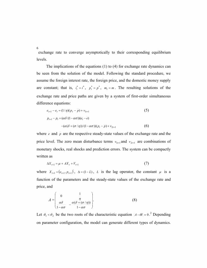
6 exchange rate to converge asymptotically to their corresponding equilibrium
levels.
The implications of the equations (1) to (4) for exchange rate dynamics can
be seen from the solution of the model. Following the standard procedure, we
assume the foreign interest rate, the foreign price, and the domestic money supply
are constant; that is, ** iit = , ** ppt = , mmt = . The resulting solutions of the
exchange rate and price paths are given by a system of first-order simultaneous
difference equations:
111 ))(/1( ++ +−=− tttt vppee η (5)
)))(1/((1 eepp ttt −−=−+ ασαδ
12)))(1/())/((( ++−−+− tt vppασησδα (6)
where e and p are the respective steady-state values of the exchange rate and the
price level. The zero mean disturbance terms 11 +tv and 12 +tv are combinations of
monetary shocks, real shocks and prediction errors. The system can be compactly
written as
11 ++ ++=∆ ttt VAXX µ (7)
where ( )'111 , +++ = ttt peX , )1( L−=∆ , L is the lag operator, the constant µ is a
function of the parameters and the steady-state values of the exchange rate and
price, and
A =
−+
−− ασ
ησδαασ
αδη
1))/((
1
10. (8)
Let 21 θθ < be the two roots of the characteristic equation 0=− IA θ .2 Depending
on parameter configuration, the model can generate different types of dynamics.
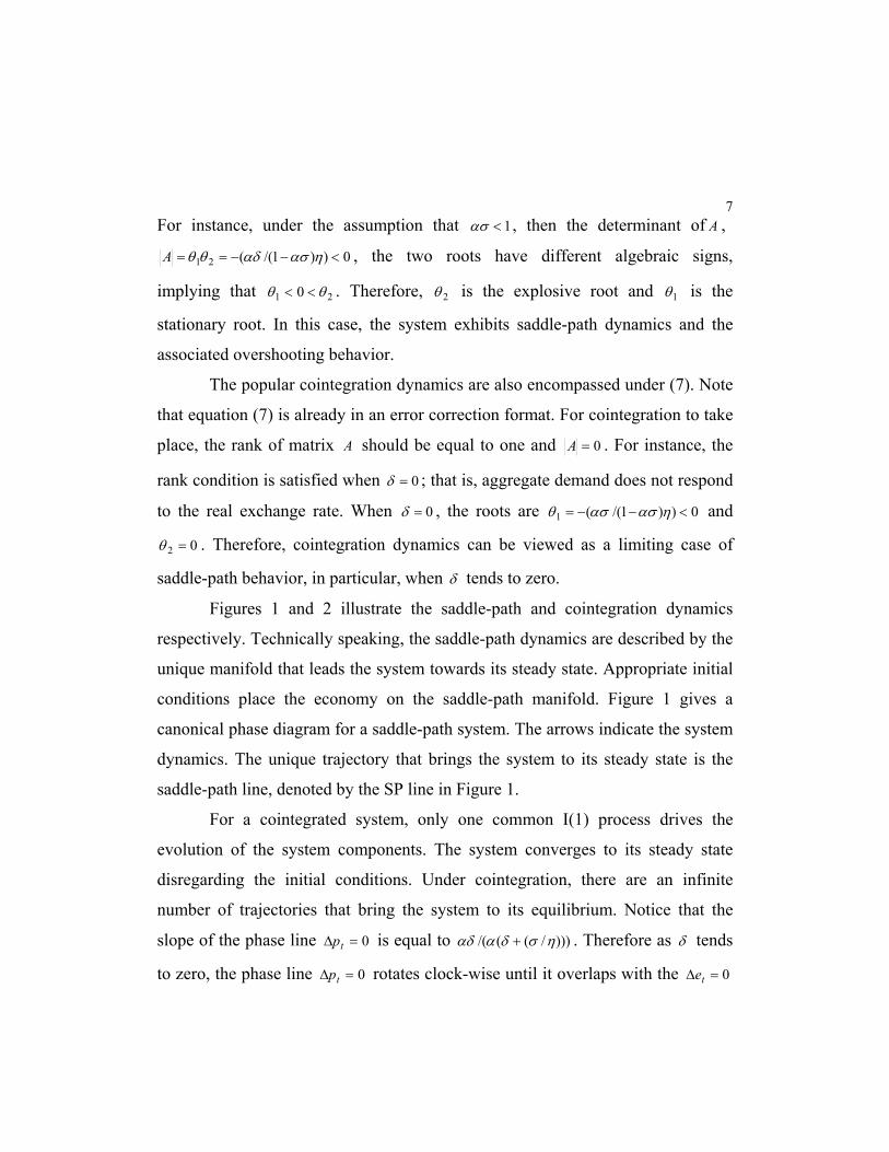
7For instance, under the assumption that 1<ασ , then the determinant of A ,
0))1/((21 <−−== ηασαδθθA , the two roots have different algebraic signs,
implying that 21 0 θθ << . Therefore, 2θ is the explosive root and 1θ is the
stationary root. In this case, the system exhibits saddle-path dynamics and the
associated overshooting behavior.
The popular cointegration dynamics are also encompassed under (7). Note
that equation (7) is already in an error correction format. For cointegration to take
place, the rank of matrix A should be equal to one and 0=A . For instance, the
rank condition is satisfied when 0=δ ; that is, aggregate demand does not respond
to the real exchange rate. When 0=δ , the roots are 0))1/((1 <−−= ηασασθ and
02 =θ . Therefore, cointegration dynamics can be viewed as a limiting case of
saddle-path behavior, in particular, when δ tends to zero.
Figures 1 and 2 illustrate the saddle-path and cointegration dynamics
respectively. Technically speaking, the saddle-path dynamics are described by the
unique manifold that leads the system towards its steady state. Appropriate initial
conditions place the economy on the saddle-path manifold. Figure 1 gives a
canonical phase diagram for a saddle-path system. The arrows indicate the system
dynamics. The unique trajectory that brings the system to its steady state is the
saddle-path line, denoted by the SP line in Figure 1.
For a cointegrated system, only one common I(1) process drives the
evolution of the system components. The system converges to its steady state
disregarding the initial conditions. Under cointegration, there are an infinite
number of trajectories that bring the system to its equilibrium. Notice that the
slope of the phase line 0=∆ tp is equal to )))/((/( ησδααδ + . Therefore as δ tends
to zero, the phase line 0=∆ tp rotates clock-wise until it overlaps with the 0=∆ te

8 phase line. Figure 2 depicts the phase diagram of a cointegrated system, where
the two lines overlap. When δ tends to zero, the explosive region in Figure 1
disappears and there is an infinite number of paths leading to the line where the
two phase lines overlap. The manifold where the two phase lines overlap is
known as the “attractor” of the system.
Figure 9.1 Saddle Path Dynamics

9
Figure 2 Cointegration Dynamics
There is another case that deserves attention. When 0=α , the price level
follows a random walk (a martingale difference process, to be precise), the rank
of matrix A is null, and there is no cointegration between prices and exchange
rates. Apparently, this case is not relevant to empirical data on exchange rates and
prices examined in Section 4 because these data are typically non-stationary and
prices do not follow a martingale.
3. Detecting Saddle-path Behavior
The discussion in the previous section suggests that the rank of A can be
used to infer the dynamics of the system. Instead of deriving a new testing

10method, we observe that the Johansen’s procedure, which is a standard test for
cointegration, uses the rank of A to infer the system dynamics. Thus, we explore
the possibility of using the Johansen’s procedure to discriminate the saddle-path
and stationary systems from a cointegrated system.
For a bivariate difference-stationary system, the Johansen procedure is
usually implemented as follows. First, the maximum eigenvalue statistic of the
Johansen procedure tests the null hypothesis 0)(:0 =ArankH against the
alternative 1)(:1 =ArankH . Under 0H , the unit root components of two individual
series are driven by two different )1(I processes and there is no cointegration.
Under 1H , the variables are cointegrated and the two variables are driven by one
common )1(I process and one stationary process. If 0H is rejected, the procedure
then considers the hypothesis 1)(:1 =ArankH against the alternative
2)(:2 =ArankH . While the cointegration dynamics is consistent with the non-
rejection of 1H , either a stationary system or a saddle-path system implies A has
full rank. It is interesting to recall that, in the previous section, it is shown that a
cointegration system can be interpreted as a limiting case of either a saddle-path
system or a stationary system.
In the literature, there are several studies examining the empirical
performance of the Johansen procedure (Cheung and Lai, 1993b; Gonzalo 1994).
Typically these studies consider the cointegration rather than the saddle-path
alternative. The Johansen procedure is constructed to test for the rank of A and, at
least theoretically, can be used to detect saddle-path behavior. The natural
question to ask is - "What is the empirical power of the Johansen’s tests against
the saddle-path alternative?" A Monte Carlo experiment is designed to shed some

11insights on the power issue. Again, a bivariate system that has the form of (7) is
used to illustrate the point.
TABLE 1. The Empirical Power of the Johansen Maximum Eigenvalue Statistic Against Saddle-Path Alternatives
Roots T = 100 T = 300
θ2 θ1 10vsHH 21vsHH 10vsHH 21vsHH 0.20 -0.20 1.0 0.7845 1.0 1.0 0.20 -0.10 1.0 0.5119 1.0 0.9944 0.20 -0.01 1.0 0.1027 1.0 0.2023 0.10 -0.20 1.0 0.5186 1.0 0.9936 σ0=0.0 0.10 -0.10 1.0 0.3703 1.0 0.9508 0.10 -0.01 1.0 0.1087 1.0 0.1977 0.01 -0.20 1.0 0.1120 1.0 0.2004 0.01 -0.10 1.0 0.1244 1.0 0.1938 0.01 -0.01 1.0 0.1686 1.0 0.1566 0.20 -0.20 0.9995 0.8355 1.0 1.0 0.20 -0.10 0.9715 0.5779 1.0 0.9980 0.20 -0.01 0.9283 0.1114 1.0 0.1956 0.10 -0.20 0.9981 0.5565 1.0 0.9974 σ0=0.1 0.10 -0.10 0.8976 0.4221 1.0 0.9640 0.10 -0.01 0.7304 0.1391 1.0 0.1867 0.01 -0.20 0.9943 0.1148 1.0 0.2052 0.01 -0.10 0.7893 0.1313 1.0 0.2028 0.01 -0.01 0.4326 0.1301 0.7625 0.1688 0.20 -0.20 0.8881 0.9573 1.0 1.0 0.20 -0.10 0.5943 0.8082 1.0 0.9995 0.20 -0.01 0.5732 0.0343 1.0 0.0521 0.10 -0.20 0.8253 0.7037 1.0 0.9997 σ0=1.0 0.10 -0.10 0.3279 0.5974 1.0 0.9939 0.10 -0.01 0.2619 0.0672 0.9487 0.0544 0.01 -0.20 0.8304 0.1163 1.0 0.2014 0.01 -0.10 0.2393 0.2173 1.0 0.1997 0.01 -0.01 0.2429 0.0543 0.2119 0.1369

12
TABLE 1 Continued. Roots T = 100 T = 300 θ2 θ1 10vsHH 21vsHH 10vsHH 21vsHH
0.20 -0.20 0.7946 0.9911 1.0 1.0 0.20 -0.10 0.4929 0.9503 1.0 1.0 0.20 -0.01 0.4770 0.0027 1.0 0.0057 0.10 -0.20 0.7024 0.7809 1.0 1.0 σ0=10.0 0.10 -0.10 0.2123 0.7612 1.0 0.9999 0.10 -0.01 0.1951 0.0046 0.9017 0.0065 0.01 -0.20 0.7479 0.1223 1.0 0.2087 0.01 -0.10 0.1465 0.2874 1.0 0.2077 0.01 -0.01 0.2180 0.0234 0.1244 0.0748
Note to Table 1: The empirical rejection frequencies of applying the Johansen maximum eigenvalue test to artificial data generated according to saddle-path dynamics are reported. The rejection frequencies are based on 10,000 replications and a 5% critical value. Two sample sizes; T = 100 and T = 300, are considered. The hypotheses are defined by H0: rank(A) = 0, H1: rank(A) = 1, and H2: rank(A) = 2. Two rejection frequencies are recorded. The first one reported under the column " 10vsHH " is the frequency of H0 being rejected. The second one reported under " 10vsHH " is the frequency of H1 being rejected conditioning on the rejection of H0. The characteristic roots of the system are given by θ1 and θ2. The standard deviation of the initial condition is given by 0σ . See the text for a more detailed description of the simulation.
The Monte Carlo experiment is conducted as follows. First, T
observations of tX are generated according to saddle-path dynamics. The
Appendix contains information on the procedure used to generate the data.
Second, the maximum eigenvalue statistic is used to test the hypothesis
0)(:0 =ArankH against the alternative 1)(:1 =ArankH . If 0H is rejected in favor of
1H , then 1H is tested against the alternative 2)(:2 =ArankH . Third, the procedure
is repeated N times. Two rejection frequencies are recorded. The first one is the
frequency of 0H being rejected. The second one is the frequency of 1H being
rejected, conditioning on the rejection of 0H . The following parameter values are

13considered: T = (100, 300), N = 10,000, 1θ = (-0.20, -0.1, -0.01), 2θ = (0.20,
0.1, 0.01), and 01.0)var(2 == iti νσ . An additional parameter is the variance of the
distribution ( 20σ ) from which the initial observation is drawn. The values of 0σ
used in the experiment are 0, 0.1, 1, and 10.
Because the Johansen’s methodology is a standard test procedure, we refer
the reader to, for example, Johansen and Juselius (1990), for a detailed discussion
of the procedure and of the construction of the maximum eigenvalue statistic.
The simulations results are reported in Table 1. The rejection frequencies
are derived using the 5% critical value. One relatively easy to interpret result is
that the power increases with the sample size. Conditional on the other parameter
values, the rejection frequency increases with the sample size – that is, the test is
consistent. The implications of the roots 1θ and 2θ for the rejection frequencies
are quite intuitive. In general, the further away the roots are from zero, the higher
is the rejection frequency. Exceptions occur when T = 100, 1θ = -0.01 and 2θ =
0.01. In some of these cases, the rejection frequency for 1H against 2H is higher
than in some other parameter combinations in which the roots are further away
from zero. However, the apparent odd result disappears when the rejection
frequency for 1H against 2H is computed without conditioning on the rejection of
0H .
It is interesting to observe that, for the two tests 0H against 1H and 1H
against 2H , both 1θ and 2θ have comparable effects on the rejection frequencies.
The observation is consistent with the fact that the Johansen procedure is a test for
the rank of the relevant coefficient matrix. When either 1θ or 2θ is approaching
zero, the rank of the relevant matrix is approaching one, the system dynamics are

14shifting towards 1H , and it is getting more and more difficult to reject 1H . As a
general rule, when both 1θ and 2θ are close to zero, the rank is close to zero and
the test has low power to reject 0H . It is not too surprising to observe the limited
power of the test, especially when 1θ = -0.01 and 2θ = 0.01. Statistical tests always
have low power for alternatives that are very close to the null hypothesis.
The effect of 0σ appears intricate. When 00 =σ , all simulated time series
are initially at the steady state. The system moves away from the steady state in
the presence of random shocks and, then, follows the saddle-path to the new
steady state. When 00 >σ , the initial position of the system is not necessarily at
the steady state. The greater 0σ , the more likely the system is initially far away
from the steady state. In fact, the 0σ parameter can have two opposite effects on
the empirical power. On the one hand, when 0σ is large, the initial shock moves
the system far away from the steady state and, hence, the system stays for a long
time on the converging saddle path. Intuitively, it would be easier for the test to
reveal the saddle-path dynamics. On the other hand, a large 0σ introduces a high
level of noise and, subsequently, makes it more difficult to reject the
nonstationarity (null) hypothesis and less easy to uncover saddle-path dynamics.
The results in Table 1 indicate that the effect of 0σ depends on the roots
1θ and 2θ . It is instructive to compare the two extremes cases ( 1θ = -0.20 and 2θ =
0.20) and ( 1θ = -0.01 and 2θ = 0.01). In the former case, the roots are quite
different from zero and the system is far away from 0H and 1H . An increase in the
value of 0σ from 0 to 1 is accompanied with an increase in the number of cases in
which favorable evidence is gardened for 2H . The result holds when either the
conditional rejection frequency (the one reported in the table) or the total rejection

15frequency is considered. Thus, for this parameter configuration, an increase in
the value of 0σ from 0 to 1 improves the ability to detect saddle-path dynamics.
The rejection frequency falls, however, when 0σ is increased from 1 to 10. Thus,
when the noise level associated with 0σ is high (relative to the distance from 0H
and 1H ), 0σ negatively affects the power of the test to detect saddle-path
dynamics. For the case 1θ = -0.01 and 2θ = 0.01, the system is very close to having
two zero roots. Under this situation, an increase in the value of 0σ makes it more
difficult to discern the saddle-path dynamics and, thus, lowers the ability of the
test to reject 0H and 1H . The positive (negative) effect of 0σ on ability to reveal
saddle-path dynamics dominates when the system dynamics is far away from
(close to) those implied by 0H and 1H .
TABLE 2. The Empirical Power of the Johansen Maximum Eigenvalue Statistic Against Stationary Alternatives
Roots T = 100 T = 300 θ2 θ1 Ho Vs
H1 H1 Vs H2 Ho Vs
H1 H1 Vs H2
-0.20 -0.20 1.0 0.8349 1.0 1.0 -0.20 -0.10 1.0 0.5641 1.0 0.9974 -0.20 -0.01 1.0 0.1042 1.0 0.1972 -0.10 -0.20 1.0 0.5485 1.0 0.9975 -0.10 -0.10 1.0 0.3980 1.0 0.9613 -0.10 -0.01 1.0 0.1135 1.0 0.1862 -0.01 -0.20 1.0 0.1064 1.0 0.2028 -0.01 -0.10 1.0 0.1128 1.0 0.1939 -0.01 -0.01 1.0 0.1326 1.0 0.1551
Notes to Table 2: The empirical rejection frequencies of applying the Johansen maximum eigenvalue test to artificial data generated according to stationary dynamics are reported. The rejection frequencies are based on 10,000 replications and a 5% critical value. Two sample sizes;

16T = 100 and T = 300, are considered. The hypotheses are defined by H0: rank(A) = 0, H1:
rank(A) = 1, and H2: rank(A) = 2. Two rejection frequencies are recorded. The first one reported under the column “ 10vsHH ” is the frequency of H0 being rejected. The second one reported under " 21vsHH " is the frequency of H1 being rejected conditioning on the rejection of H0. The characteristic roots of the system are given by θ1 and θ2. See the text for a more detailed description of the simulation.
In conducting the simulation experiment, the Johansen trace statistics were
also computed. However, the empirical power estimates based on the trace
statistic are very similar to those based on the maximum eigenvalue statistic.
Different values of 21σ and 2
2σ were also included in the experiment. It turns out
that the simulation results are quite insensitive to a) the value of 21σ and 2
2σ , and
b) the relative size of of 21σ and 2
2σ . Thus, the simulation results related to the
trace statistic and different combinations of 21σ and 2
2σ are not reported for
brevity. These results are available from the authors upon request.
While the results indicate that the Johansen procedure has a reasonable
power to uncover saddle-path behavior, it is noted that a stationary bivariate
system can lead to similar rejection results. It is instructive to assess the power of
the test in the presence of stationary data. To this end, we apply the Johansen
procedure to data generated under stationary alternatives. The stationary roots
considered are 1θ , 2θ = (-0.2, -0.10, -0.01). The other parameters are the same as
those considered in Table 1. Table 2 reports the power of the Johansen procedure
against the stationary alternatives when we set 00 =σ .
Similar to the saddle-path experiment, the empirical power in Table 2 is
increasing with the sample size and the distance of the roots from zero. Compared
with results in Table 1, results in Table 2 indicate that the Johansen maximum

17eigenvalue statistic has reasonable power in detecting the full rank condition –
no matter it is generated by saddle-path or stationary dynamics.
4. Exchange Rate Dynamics
In this section, we use the Johansen procedure to infer whether the saddle-
path and the related overshooting dynamics are an appropriate description of
exchange rate dynamics. Four dollar-based exchange rates namely British pound,
French franc, German mark, and Italian lira are included in the sample. Monthly
data of nominal exchange rates and consumer price indexes from April 1973 to
December 1998 were retrieved from the International Financial Statistics data
CD-ROM. These data are expressed in logarithms. As commonly conceived, the
individual exchange rate and price series display I(1) non-stationarity. Following
the literature, the bivariate system comprising of the nominal exchange rate and
the relative price is employed to study the cointegration relationship between
exchange rates and relative prices.
For notational purposes, a bivariate system as (7) is re-writen in its general
form:
tk
i ititt VXAAXX ∑ −
= −− +++=∆1
11µ (9)
where no parameter restriction is imposed on matrices A and iA . The lagged tX ’s
are included to ensure that tV follows a white noise process and that the Johansen
result is not distorted by serial correlation in the error term. In implementing the
test, the lag parameter k is selected using the Akaike information criterion. Both
the Johansen maximum eigenvalue and trace statistics are calculated. Again we
refer readers to Johansen and Juselius (1990) for the construction of these test
statistics.

18
TABLE 3. Johansen cointegration test results Max. Eigenvalue Stat. Trace Stat. Rank(A) =
0 Rank(A) = 1
Rank(A) = 0
Rank(A) = 1
British Pound Lag = 2 21.3878* 5.3478 26.7356* 5.3478 French Franc Lag = 4 34.7165* 4.3357 39.0522* 4.3357 German Mark Lag = 1 15.9658** 3.9937 19.9595* 3.9937 Italian Lira Lag = 1 26.6205* 4.9276 31.5481* 4.9276
Notes to Table 3: The Johansen tests for cointegration between nominal exchange rates and relative prices are presented. Both the maximum eigenvalue statistic "Max. Eigenvalue Stat." and the trace statistics "Trace Stat." are reported. The null hypotheses are given underneth the statistic labels. The alternatives for the maximum eigenvalue statistic are Rank(A) = 1 and Rank(A) = 2 and the those for the trace statistic are Rank(A) > 0 and Rank(A) > 1. The lag paramter "Lag =" is selected using the Akaike information criterion. Significance at the 5% and 1% levels are indicated by "**" and "*" according to the finite sample critical values in Cheung and Lai (1993b). The hypothesis of Rank(A) = 0 is rejected by both statistics but the hypothesis of Rank(A) = 1 is not rejected.
The results of the Johansen tests are reported in Table 3. Both the
maximum eigenvalue and trace statistics reject the null hypothesis 0)(:0 =ArankH
but not the null hypothesis 1)(:1 =ArankH . Thus, the exchange rate and the
relative price are cointegrated and the two series in each bivariate system are
driven by a common I(1) process. Individually, each series evolves as a non-
stationary I(1) process. However, a unique combination of the two series
governed by the cointegrating vector is stationary. Typically, the cointegration

19result is interpreted as the evidence of the presence of an empirical long-run
relationship between exchange rates and prices, which constitutes a necessary
condition for long-run purchasing power parity (Cheung and Lai, 1993a; Kugler
and Lenz, 1993).
The results in the previous sections allow us to use the rank of A to infer
the system dynamics from a different perspective. In addition to the long-run
relationship interpretation, our results also indicate that neither the notion of
saddle-path nor stationary dynamics are consistent with the inference that the rank
of A is equal to one. Because exchange rates and relative prices are I(1) processes,
the bivariate system consisting of these two variables is not stationary. Thus, the
strength of the result is its implications for the irrelevance of using saddle-path
and the related overshooting dynamics to describe exchange rate behavior.
There are a few caveats in generalizing the cointegration results. First, the
empirical illustration includes only a few countries even though these are the key
industrial countries. It is fair to say that a more definite inference on the relevancy
of saddle-path dynamics still awaits additional results from a larger set of dollar-
based exchange rates and cross-rates. Second, as indicated in the simulation
experiment, the ability to detect saddle-path dynamics is severely handicapped
when the explosive root is very close to one. Further analyses are required to rule
out this possibility. Nonetheless, the cointegration results in Table 3 cast doubt on
the general validity of saddle-path/overshooting exchange rate dynamics.
5. Concluding Remarks
The overshooting model à la Dornbusch is a prominent explanation for the
volatile exchange rate behavior in the current floating period. Assuming prices are

20sticky, the model displays a saddle-path pattern and yields overshooting
dynamics that induces high short-term exchange rate volatility. Using a bivariate
system, this study illustrates the implications of saddle-path, cointegration, and
stationary dynamics for the characteristic roots that determines the system’s
intertemporal behavior. It is shown that a cointegration system can be interpreted
as a limiting case of a system that displays either saddle-path or stationarity
dynamics. A Monte Carlo experiment is designed to illustrate the usefulness of
the Johansen tests to uncover saddle-path dynamics. The simulation results
indicate that the Johansen tests have a) reasonable power to detect saddle-path
dynamics, and b) similar power to reject the cointegration hypothesis in favor of
saddle-path or stationarity alternatives.
Our empirical example shows that exchange rates and prices are
cointegrated. Because the variables in a saddle-path system are not supposed to
display a cointegrating relationship, the empirical evidence is indicative of the
absence of saddle-path dynamics in the data under investigation. Exchange rate
models that do not rely on saddle-path properties and over-shooting dynamics
may deserve some more serious attention.
It is conceivable that the implications of the current study go beyond the
exchange rate saddle-path behavior. There are models in different areas in
economics exhibiting saddle-path properties. For instance, the neo-classical
growth model (Cass, 1965) is an early example in which saddle-path dynamics
are used to elaborate balanced-growth. Other models that utilize saddle-path
dynamics to elucidate relationships between economic variables include those of
Bruno and Fischer (1991) for interest rates and inflation, Evans and Yarrow
(1981) for real money balances and inflation. The saddle-path property in these
models, however, is not commonly subject to direct empirical test.

21Nonetheless, it is noted that some studies report cointegrating
relationship between a) output, investment, and consumption (King et al., 1991)3
and between interest rates and inflation (Bonham; 1991). These cointegration
results imply the saddle-path models may not be appropriate for these variables.
While the Johansen procedure, as illustrated in previous sections, can be
used to test for saddle-path dynamics, further studies on other testing procedures
for saddle-path dynamics are warranted; especially given the widespread use of
saddle-path models in economics.

22
Appendix: Generating Data that Exhibit Saddle-Path Dynamics
The simulation experiment dealing with saddle-path dynamics is
conducted as follows. First, we find a solution to equation (7) under the saddle-
path hypothesis. Second, using the saddle-path solution, we simulate tX of length
T . T = 100 and T = 300 are considered in the exercise. Third, the Johansen test
statistic is calculated from the simulated data. The above steps are repeated N
times and N is set to 10,000. The N sample Johansen statistics are then
compared with the 5% critical value to tally the rejection frequency.
We follow the standard procedure to obtain the saddle-path solution to
equation (7). Let B be a (2x2) matrix whose columns contain the eigenvectors of
)( IA + . Pre-multiplying system (7) by 1−B , we obtain ttt UZZ +Λ= −1 where
tt XBZ 1−= , )(1 IAB +=Λ − is a diagonal matrix with the eigenvalues of )( IA+
along the diagonal and tt VBU 1−= . Then, we solve each of the first-order
difference equations ititiit uzz ++= −1)1( θ ; 2,1=i where )',( 21 ttt zzZ = and
)',( 21 ttt uuU = . Under the saddle-path hypothesis, 01 <θ and 02 >θ . We solve the
first equation backward and the second equation forward. The solutions can be
expressed as the sum of two terms:
0* )1( i
tiitit czz θ++=
where
∑∞
=−+=
011
*1 )1(
iit
it uz θ ,
∑∞
=++
+
+
=0
12
1
2
*2 1
1
iit
i
t uzθ

23and *
000 iii zzc −= . In economics, these two terms are usually labeled the "steady
state" and the "bubble." The saddle-path solution is obtained by setting the
terminal condition 020 =c so that the resulting sequence is not explosive. The
original variables of the system are then recovered using tt BZX = .
The steady state )',( *2
*1
*ttt zzZ = is approximated by the sum of a finite
number of elements. We first generate the series tU of length T3 using a normal
random number generator. The first T simulated numbers are used to generate *11z , the first 1+T simulated numbers are used to generate *
12z , ..., and so on. The
last T simulated numbers are used to generate *2Tz , the last 1+T simulated
numbers are used to generate *12 −Tz , …, and so on. In addition, the initial
condition 10c is required to calculate the solution. In the experiment, the initial
condition 10c is drawn from a normal distribution with zero mean and variance
20σ . The idea of the random choice is to capture the existence of a continuum of
equilibria (each indexed by a different initial condition) lying on the unique stable
manifold converging to the steady state.

24
References
Azariadis, C., 1993, Intertemporal Macroeconomics, Blackwell Publisher,
Oxford.
Bonham, C., 1991, Correct Cointegration Tests of the Long-Run Relationship
between Nominal Interest and Inflation, Applied Economics 23, 1487-
1492
Bruno, M. and S. Fischer, 1991, Seigniorage, Operating Rules, and the High
Inflation Trap, Quarterly Journal of Economics 105, 353-374.
Cass, D., 1965, Optimum Growth in an Aggregative Model of Capital
Accumulation, Review of Economic Studies 32, 233-240.
Cheung, Y.-W. and K.S. Lai ,1993a, Long-Run Purchasing Power Parity During
the Recent Float, Journal of International Economics 34, 181-192.
Cheung, Y.-W. and K.S. Lai ,1993b, Finite-Sample Sizes of Johansen's
Likelihood Ratio Tests for Cointegration, Oxford Bulletin of Economics
and Statistics 55, 313-328.
Cheung, Y.-W. and K.S. Lai, 2000, On the Purchasing Power Parity Puzzle,
Journal of International Economics 52, 321-330.
Cheung, Y.-W., S. Lai and M. Bergman, 2004, Dissecting the PPP Puzzle: The
Unconventional Roles of Nominal Exchange Rate and Price Adjustments,
Journal of International Economics (forthcoming).
Clarida, R. and J. Gali, 1994, Sources of Real Exchange Fluctuations: How
Important are Nominal Shocks?, Carnegie-Rochester Conference Series
on Public Policy 41, 1-56.
Dornbusch, R., 1976, Expectations and Exchange Rate Dynamics, Journal of
Political Economy 84, 1161-1176.

25Driskill, R.A., 1981, Exchange Rate Dynamics, An Empirical Analysis, Journal
of Political Economy 89, 357-371.
Driskill, R.A. and S.M. Sheffrin, 1981, On the Mark: Comment, American
Economic Review 71, 1068-1074.
Edison, H.J. and B.D. Pauls, 1993, A Re-Assessment of the Relationship between
Real Exchange Rates and Real Interest Rates : 1974-1990, Journal of
Monetary Economics 31, 165-87.
Eichenbaum, M. and C.L. Evans, 1995, Some Empirical Evidence on the Effects
of Shocks to Monetary Policy on Exchange Rates, Quarterly Journal of
Economics 110, 975-1009.
Engel, C. and J.C. Morley, 2001, The Adjustment of Prices and the Adjustment of
the Exchange Rate, manuscript, University of Wisconsin.
Evans, J. and G. Yarrow, 1981, Some Implications of Alternative Expectations
Hypotheses in the Monetary Analysis of Hyperinflations, Oxford
Economic Papers 33, 61-80.
Faust, J., 1998, The Robustness of Identified VAR Conclusions About Money,
Carnegie-Rochester Conference Series on Public Policy 41, 1-56
Faust, J. and J.H. Rogers, 1999, Monetary Policy's Role in Exchange Rate
Behavior, International Finance Discussion Paper #652, Board of
Governors of the Federal Reserve System.
Frankel, J., 1979, On the Mark: A Theory of Floating Exchange Rates Based on
Real Interest Differentials, American Economic Review 69, 610-622.
Frankel, J. and A. Rose, 1995, Empirical Research on Nominal Exchange Rates,
Chapter 33 in G. Grossman and K. Rogoff, eds., Handbook of Internationl
Economics Vol. 3, 1689-1729, Elsevier - Amsterdam.

26Gonzalo, J., 1994, Five Alternative Methods of Estimating Long-Run
Equilibrium Relationships, Journal of Econometrics 60, 203-33.
Johansen, S. and K. Juselius, 1990, Maximum Likelihood Estimation and
Inference on Cointegration--With Applications to the Demand for Money,
Oxford Bulletin of Economics and Statistics 2, 169-210.
King, R., C. Plosser, J. Stock and M. Watson, 1991, Stochastic Trends and
Economic Fluctuations, American Economic Review 81, 819-40.
Kugler, P. and C. Lenz, 1993, Multivariate Cointegration Analysis and the Long-
Run Validity of PPP, Review of Economics and Statistics 75, 180-184.
Meese, R. and K. Rogoff, 1988, Was it Real? The Exchange Rate-Interest Rate
Differential Relation over the Modern Floating-Rate Period, The Journal
of Finance 43, 933-948.

27Notes. 1 Strictly speaking, overshooting implies saddle-path but the opposite is not true. 2 Notice that if equation (7) is written as 11 ++ +Π+= ttt VXX µ , where IA+=Π ,
then the roots ofΠ , say 1λ and 2λ , are related to the roots of A according to
ii θλ +=1 , i=1,2. Therefore, a unit root of Π is equivalent to a zero root of A . 3 King et al. (1991) show in a neoclassical growth framework that (the logs of)
output, consumption and investment are cointegrated when thechnology shocks
follow an I(1) process, whereas certain ratios characterizing the balanced-growth
path (for instance, the consumption-output and the investment-output great ratios)
exhibit saddle-path dynamics.

CESifo Working Paper Series (for full list see www.cesifo.de)
________________________________________________________________________ 1061 Helmuth Cremer and Pierre Pestieau, Wealth Transfer Taxation: A Survey, October
2003 1062 Henning Bohn, Will Social Security and Medicare Remain Viable as the U.S.
Population is Aging? An Update, October 2003 1063 James M. Malcomson , Health Service Gatekeepers, October 2003 1064 Jakob von Weizsäcker, The Hayek Pension: An efficient minimum pension to
complement the welfare state, October 2003 1065 Joerg Baten, Creating Firms for a New Century: Determinants of Firm Creation around
1900, October 2003 1066 Christian Keuschnigg, Public Policy and Venture Capital Backed Innovation, October
2003 1067 Thomas von Ungern-Sternberg, State Intervention on the Market for Natural Damage
Insurance in Europe, October 2003 1068 Mark V. Pauly, Time, Risk, Precommitment, and Adverse Selection in Competitive
Insurance Markets, October 2003 1069 Wolfgang Ochel, Decentralising Wage Bargaining in Germany – A Way to Increase
Employment?, November 2003 1070 Jay Pil Choi, Patent Pools and Cross-Licensing in the Shadow of Patent Litigation,
November 2003 1071 Martin Peitz and Patrick Waelbroeck, Piracy of Digital Products: A Critical Review of
the Economics Literature, November 2003 1072 George Economides, Jim Malley, Apostolis Philippopoulos, and Ulrich Woitek,
Electoral Uncertainty, Fiscal Policies & Growth: Theory and Evidence from Germany, the UK and the US, November 2003
1073 Robert S. Chirinko and Julie Ann Elston, Finance, Control, and Profitability: The
Influence of German Banks, November 2003 1074 Wolfgang Eggert and Martin Kolmar, The Taxation of Financial Capital under
Asymmetric Information and the Tax-Competition Paradox, November 2003 1075 Amihai Glazer, Vesa Kanniainen, and Panu Poutvaara, Income Taxes, Property Values,
and Migration, November 2003

1076 Jonas Agell, Why are Small Firms Different? Managers’ Views, November 2003 1077 Rafael Lalive, Social Interactions in Unemployment, November 2003 1078 Jean Pisani-Ferry, The Surprising French Employment Performance: What Lessons?,
November 2003 1079 Josef Falkinger, Attention, Economies, November 2003 1080 Andreas Haufler and Michael Pflüger, Market Structure and the Taxation of
International Trade, November 2003 1081 Jonas Agell and Helge Bennmarker, Endogenous Wage Rigidity, November 2003 1082 Fwu-Ranq Chang, On the Elasticities of Harvesting Rules, November 2003 1083 Lars P. Feld and Gebhard Kirchgässner, The Role of Direct Democracy in the European
Union, November 2003 1084 Helge Berger, Jakob de Haan and Robert Inklaar, Restructuring the ECB, November
2003 1085 Lorenzo Forni and Raffaela Giordano, Employment in the Public Sector, November
2003 1086 Ann-Sofie Kolm and Birthe Larsen, Wages, Unemployment, and the Underground
Economy, November 2003 1087 Lars P. Feld, Gebhard Kirchgässner, and Christoph A. Schaltegger, Decentralized
Taxation and the Size of Government: Evidence from Swiss State and Local Governments, November 2003
1088 Arno Riedl and Frans van Winden, Input Versus Output Taxation in an Experimental
International Economy, November 2003 1089 Nikolas Müller-Plantenberg, Japan’s Imbalance of Payments, November 2003 1090 Jan K. Brueckner, Transport Subsidies, System Choice, and Urban Sprawl, November
2003 1091 Herwig Immervoll and Cathal O’Donoghue, Employment Transitions in 13 European
Countries. Levels, Distributions and Determining Factors of Net Replacement Rates, November 2003
1092 Nabil I. Al-Najjar, Luca Anderlini & Leonardo Felli, Undescribable Events, November
2003 1093 Jakob de Haan, Helge Berger and David-Jan Jansen, The End of the Stability and
Growth Pact?, December 2003
1094 Christian Keuschnigg and Soren Bo Nielsen, Taxes and Venture Capital Support, December 2003
1095 Josse Delfgaauw and Robert Dur, From Public Monopsony to Competitive Market.
More Efficiency but Higher Prices, December 2003 1096 Clemens Fuest and Thomas Hemmelgarn, Corporate Tax Policy, Foreign Firm
Ownership and Thin Capitalization, December 2003 1097 Laszlo Goerke, Tax Progressivity and Tax Evasion, December 2003 1098 Luis H. B. Braido, Insurance and Incentives in Sharecropping, December 2003 1099 Josse Delfgaauw and Robert Dur, Signaling and Screening of Workers’ Motivation,
December 2003 1100 Ilko Naaborg,, Bert Scholtens, Jakob de Haan, Hanneke Bol and Ralph de Haas, How
Important are Foreign Banks in the Financial Development of European Transition Countries?, December 2003
1101 Lawrence M. Kahn, Sports League Expansion and Economic Efficiency: Monopoly Can
Enhance Consumer Welfare, December 2003 1102 Laszlo Goerke and Wolfgang Eggert, Fiscal Policy, Economic Integration and
Unemployment, December 2003 1103 Nzinga Broussard, Ralph Chami and Gregory D. Hess, (Why) Do Self-Employed
Parents Have More Children?, December 2003 1104 Christian Schultz, Information, Polarization and Delegation in Democracy, December
2003 1105 Daniel Haile, Abdolkarim Sadrieh and Harrie A. A. Verbon, Self-Serving Dictators and
Economic Growth, December 2003 1106 Panu Poutvaara and Tuomas Takalo, Candidate Quality, December 2003 1107 Peter Friedrich, Joanna Gwiazda and Chang Woon Nam, Development of Local Public
Finance in Europe, December 2003 1108 Silke Uebelmesser, Harmonisation of Old-Age Security Within the European Union,
December 2003 1109 Stephen Nickell, Employment and Taxes, December 2003 1110 Stephan Sauer and Jan-Egbert Sturm, Using Taylor Rules to Understand ECB Monetary
Policy, December 2003 1111 Sascha O. Becker and Mathias Hoffmann, Intra-and International Risk-Sharing in the
Short Run and the Long Run, December 2003

1112 George W. Evans and Seppo Honkapohja, The E-Correspondence Principle, January 2004
1113 Volker Nitsch, Have a Break, Have a … National Currency: When Do Monetary
Unions Fall Apart?, January 2004 1114 Panu Poutvaara, Educating Europe, January 2004 1115 Torsten Persson, Gerard Roland, and Guido Tabellini, How Do Electoral Rules Shape
Party Structures, Government Coalitions, and Economic Policies? January 2004 1116 Florian Baumann, Volker Meier, and Martin Werding, Transferable Ageing Provisions
in Individual Health Insurance Contracts, January 2004 1117 Gianmarco I.P. Ottaviano and Giovanni Peri, The Economic Value of Cultural
Diversity: Evidence from US Cities, January 2004 1118 Thorvaldur Gylfason, Monetary and Fiscal Management, Finance, and Growth, January
2004 1119 Hans Degryse and Steven Ongena, The Impact of Competition on Bank Orientation and
Specialization, January 2004 1120 Piotr Wdowinski, Determinants of Country Beta Risk in Poland, January 2004 1121 Margarita Katsimi and Thomas Moutos, Inequality and Redistribution via the Public
Provision of Private Goods, January 2004 1122 Martin Peitz and Patrick Waelbroeck, The Effect of Internet Piracy on CD Sales: Cross-
Section Evidence, January 2004 1123 Ansgar Belke and Friedrich Schneider, Privatization in Austria: Some Theoretical
Reasons and First Results About the Privatization Proceeds, January 2004 1124 Chang Woon Nam and Doina Maria Radulescu, Does Debt Maturity Matter for
Investment Decisions?, February 2004 1125 Tomer Blumkin and Efraim Sadka, Minimum Wage with Optimal Income Taxation,
February 2004 1126 David Parker, The UK’s Privatisation Experiment: The Passage of Time Permits a
Sober Assessment, February 2004 1127 Henrik Christoffersen and Martin Paldam, Privatization in Denmark, 1980-2002,
February 2004 1128 Gregory S. Amacher, Erkki Koskela and Markku Ollikainen, Deforestation, Production
Intensity and Land Use under Insecure Property Rights, February 2004 1129 Yin-Wong Cheung, Javier Gardeazabal, and Jesús Vázquez, Exchange Rate Dynamics:
Where is the Saddle Path?, February 2004