Embed Size (px)
Citation preview

Exchange Competition, Entry, and Welfare∗
Giovanni Cespa† and Xavier Vives‡
Tuesday 3rd November, 2020
Abstract
We assess the consequences for market quality and welfare of different en-try regimes and exchange pricing policies, integrating a microstructure modelwith a free-entry, exchange competition model where exchanges have marketpower in technological services. Free-entry delivers superior liquidity and wel-fare outcomes vis-a-vis an unregulated monopoly, but entry can be excessive orinsufficient. Depending on the extent of the monopolist’s technological servicesundersupply compared to the first best, a planner can achieve a higher welfarecontrolling entry or platform fees.
Keywords: Market fragmentation, welfare, endogenous market structure, platform com-
petition, Cournot with free entry, industrial organization of exchanges.
JEL Classification Numbers: G10, G12, G14
∗We thank Fabio Braga, Eric Budish, Thierry Foucault, Itay Goldstein (the Editor), Jiasun Li,Albert Menkveld, Duane Seppi, Rene Stultz, Felix Suntheim, two anonymous referees and seminarparticipants at ICEF (Moscow), Boston University, Universidad Carlos III (Madrid), Imperial College(London), Chicago Fed, University of Chicago, Northwestern, Tilburg University, Tsinghua Univer-sity, NYU (Stern), the 2018 EFA meeting (Warsaw), the 2019 AFA meeting (Atlanta), and the 2020Econometric Society World Congress (Milan) for useful comments and suggestions. Cespa acknowl-edges financial support from the Bank of England (grant no. RDC151391). Vives acknowledges thefinancial support of the Ministry of Science, Innovation and Universities (MCIU)-ECO2015-63711-P and PGC2018-096325-B-I00 (MCIU/AEI/FEDER, UE) and of the Department of Economy andKnowledge of the Generalitat de Catalunya (Ref. 2017 SGR 1244). Orestis Vravosinos and BarnaZsabo provided excellent research assistance.†Cass Business School–City, University of London, and CEPR. 106, Bunhill Row, London EC1Y
8TZ, UK. e-mail: [email protected]‡IESE Business School, Avinguda Pearson, 21 08034 Barcelona, Spain.
1

“The result is that, even while one of our fundamental mandates is to
encourage competition, the SEC has stood on the sidelines while enormous
market power has become concentrated in just a few players. . . And every
time exchanges raise prices [for exchange connections], that money comes
out of investors’ pockets, who pay more to buy and sell stocks than they
otherwise might. . . In a world where the costs of electronic connections are
constantly falling, exchanges have asked us to raise these prices over and
over again during the past three years.”
Unfair Exchange: The State of America’s Stock Markets , SEC Commis-
sioner Robert J. Jackson Jr., September 2018.
1 Introduction
Over the past two decades, governments and regulators moved to foster competition
among trading venues. This has spurred market fragmentation, contributing to a dras-
tic reduction in the cost of trading, which has benefited market participants. However,
this has also led exchanges to heighten their reliance on revenue generating activities
which price they can control better. A case in point is the provision of services such
as the sale of market data, co-location space, and fast connections to matching en-
gines.1 As suggested by the opening quotation, US regulators have voiced their concern
over the price of such “technological services,” with the SEC alleging that exchanges
exercise too much market power in their provision.
When is regulatory intervention warranted? Should a regulator set the price of
technological services and if so, how? Do merger policy and the control of exchange
entry have a role to play?
We address these issues by modelling liquidity provision as a vertical market where
“upstream” exchanges supply technological services (connectivity) to “downstream”
liquidity providers, who use them to satisfy liquidity traders’ demand for immediacy.
1“Take, for example, our rules requiring orders to be routed to the exchange that displays thenational best bid or offer [. . . which ensure] that all investors get the benefit of a competitive nationalmarket system. When the SEC enacted these rules, [. . . ] there would be cases where brokers wouldbe required to send the order to a specific exchange, leaving the broker–and [. . . ] their customer–exposed to excessive trading fees on that exchange. So we capped the fees the exchanges can charge.But facing a limit on one kind of fee, exchanges may have simply raised other fees, like the costof connecting to the exchange [. . . ] For example, one exchange, EDGX, has raised the price on itsstandard 10GB connection five times since 2010–in total, leaving the price of the connection seventimes higher than it was in that year.” (Robert J. Jackson Jr., 2018)
2

We then put the model to work by comparing the market solution, with free entry of
exchanges, with the second best solutions a regulator can implement. This allows us
to analyze the Industrial Organization of stock markets and evaluate the liquidity and
welfare effects of different regulatory measures.
We find that the competitive (price-taking) solution is generically not efficient,
since exchanges only care about the welfare of market participants whose surplus they
can appropriate (a vertical externality). Hence, exchanges’ market power may improve
or worsen welfare compared to the competitive benchmark, and regulation (conduct or
structural) can improve upon the market solution. With fee (conduct) regulation it is
optimal to have only one exchange; with entry (structural) regulation the market may
deliver excessive or insufficient entry. In this context, a connectivity capacity increase
(fee reduction) can be achieved either by fostering entry, or by directly imposing it
on the regulated monopolist, and the optimal second best regulatory intervention
revolves around a simple trade-off. A fee reduction depresses (increases) industry
profits (liquidity) to the detriment (benefit) of exchanges (market participants). When
the wedge between the first best and monopoly capacity is sufficiently large (small),
entry regulation is inferior (superior) to fee regulation.
Thus, our model provides an economics backing to the logic behind the excerpt
of SEC Commissioner Robert J. Jackson’s speech reported in the opening quotation.
Indeed, the vertical structure of the liquidity supply industry and exchanges’ market
power in offering an essential input for liquidity provision explain the mechanism by
which “[. . . ] every time exchanges raise prices, that money comes out of investors’
pockets, who pay more to buy and sell stocks than they otherwise might.” In addition,
our model suggests when raising prices is detrimental or beneficial for overall welfare.
The profit orientation of exchanges, when they converted into publicly listed com-
panies, led to regulatory intervention both in the US (RegNMS in 2005) and the EU
(Mifid in 2007), to stem their market power over trading fees. Regulation, together
with the liberalization of international capital flows and technological developments,
led in turn to an increase in fragmentation and competition among trading platforms.
Incumbent exchanges such as the NYSE reacted to increased competition by upgrad-
ing technology (e.g, creating, NYSE Arca), or merging with other exchanges (e.g., the
NYSE merged with Archipelago in 2005 and with Euronext in 2007. See Foucault
et al. (2013), Chapter 1). A relevant fact is that even though there are 13 lit stock
venues in the US (and 30 alternative ones), 12 of them, which account for two-thirds
of daily trading, are controlled by three major players: Intercontinental Exchange,
3

Nasdaq, and CBOE.
As a result, the trading landscape has changed dramatically. Large-cap stocks
nowadays commonly trade in multiple venues, a fact that has led to a decline in in-
cumbents’ market shares, giving rise to a “cross-sectional” dimension of market frag-
mentation (see Appendix B, Figure B.2). The automation of the trading process has
also spurred fragmentation along a “time-series” dimension, in that some liquidity
providers’ market participation is limited (Duffie (2010), SEC (2010)), endogenous
(Anand and Venkataraman (2016)), or impaired because of the existence of limits
to the access of reliable and timely market information (Ding et al. (2014)).2 Ad-
ditionally, trading fees have declined to competitive levels (see, e.g., Foucault et al.
(2013), Menkveld (2016), and Budish et al. (2019)), and exchanges have steered their
business models towards the provision of technological services.3
Such a paradigm shift has raised regulators’ and policy makers’ concerns for the
possibility of monopoly restrictions. Indeed, in August 2020, the SEC has rescinded
the rule that allowed exchanges to unilaterally change their “core” data fees and, from
September 2020, subjected such changes to public comment and regulatory approval.
As a result, the SEC now holds an ex-ante control over exchanges’ fee setting process.4
2Limited market participation of liquidity providers also arises because of shortages of arbitragecapital (Duffie (2010)) and/or traders’ inattention or monitoring costs (Abel et al. (2013)).
3Increasing competition in trading services has squeezed the profit margins exchanges drew fromtraditional activities, leading them to gear their business model towards the provision of technologicalservices (Cantillon and Yin (2011)). There is abundant evidence testifying to such a paradigmaticshift. For example, according to the Financial Times, “After a company-wide review Ms Friedman[Nasdaq CEO] has determined the future lies in technology, data and analytics, which collectivelyaccounted for about 35 per cent of net sales in the first half of this year.” (see, “Nasdaq’s futurelies in tech, data and analytics, says Nasdaq CEO” Financial Times, October 2017). Additionally,according to Tabb Group, in the US, exchange data, access, and technology revenues have increasedby approximately 62% from 2010 to 2015 (Tabb Group, 2016).
4In 2018, the SEC sided with market participants over their challenge to the NYSE ARCA’s andNASDAQ’s decision to increase their data fees (Statement on Market Data Fees and Market Structure,SEC Chairman J. Clayton, October 2018, Clayton, 2018, Bloomberg, 2018). Stock exchanges subse-quently appealed against the SEC’s decision, and in June 2020, won the legal battle: the US Courtof Appeals ruled “some fee increases can’t be challenged by the government after they have takeneffect.” (WSJ, 2020). As a response, in August 2020, the SEC modified its regulatory framework,rescinding the rule that allowed exchanges to unilaterally change some of their fees: from September2020, fee hikes from exchanges for “core” data require public comment and approval from the SEC(Bloomberg, 2020). Prior to this, the SEC did not have the power to approve exchanges’ fees before-hand. However, market participants were permitted to challenge them, upon which challenge, theSEC could intervene–a form of ex-post fee control. Thus, with this new regulatory approach the SECnow holds an ex-ante control over exchanges’ fee setting process, Bloomberg, 2020). An importantelement which secured the success of exchanges’ appeal in June 2020, was the fact that the SEC basedits 2018 action on a section of law that “makes no mention of fees at all,” highlighting the lack of aproper mandate to oversee competition at the core of the US regulator’s mission.
4
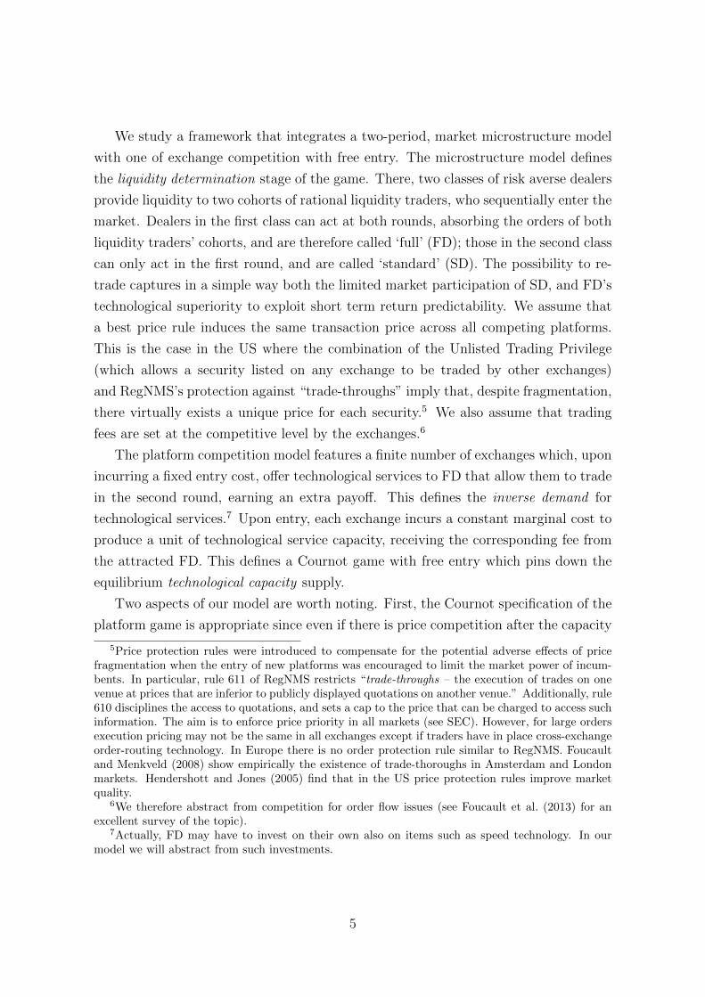
We study a framework that integrates a two-period, market microstructure model
with one of exchange competition with free entry. The microstructure model defines
the liquidity determination stage of the game. There, two classes of risk averse dealers
provide liquidity to two cohorts of rational liquidity traders, who sequentially enter the
market. Dealers in the first class can act at both rounds, absorbing the orders of both
liquidity traders’ cohorts, and are therefore called ‘full’ (FD); those in the second class
can only act in the first round, and are called ‘standard’ (SD). The possibility to re-
trade captures in a simple way both the limited market participation of SD, and FD’s
technological superiority to exploit short term return predictability. We assume that
a best price rule induces the same transaction price across all competing platforms.
This is the case in the US where the combination of the Unlisted Trading Privilege
(which allows a security listed on any exchange to be traded by other exchanges)
and RegNMS’s protection against “trade-throughs” imply that, despite fragmentation,
there virtually exists a unique price for each security.5 We also assume that trading
fees are set at the competitive level by the exchanges.6
The platform competition model features a finite number of exchanges which, upon
incurring a fixed entry cost, offer technological services to FD that allow them to trade
in the second round, earning an extra payoff. This defines the inverse demand for
technological services.7 Upon entry, each exchange incurs a constant marginal cost to
produce a unit of technological service capacity, receiving the corresponding fee from
the attracted FD. This defines a Cournot game with free entry which pins down the
equilibrium technological capacity supply.
Two aspects of our model are worth noting. First, the Cournot specification of the
platform game is appropriate since even if there is price competition after the capacity
5Price protection rules were introduced to compensate for the potential adverse effects of pricefragmentation when the entry of new platforms was encouraged to limit the market power of incum-bents. In particular, rule 611 of RegNMS restricts “trade-throughs – the execution of trades on onevenue at prices that are inferior to publicly displayed quotations on another venue.” Additionally, rule610 disciplines the access to quotations, and sets a cap to the price that can be charged to access suchinformation. The aim is to enforce price priority in all markets (see SEC). However, for large ordersexecution pricing may not be the same in all exchanges except if traders have in place cross-exchangeorder-routing technology. In Europe there is no order protection rule similar to RegNMS. Foucaultand Menkveld (2008) show empirically the existence of trade-thoroughs in Amsterdam and Londonmarkets. Hendershott and Jones (2005) find that in the US price protection rules improve marketquality.
6We therefore abstract from competition for order flow issues (see Foucault et al. (2013) for anexcellent survey of the topic).
7Actually, FD may have to invest on their own also on items such as speed technology. In ourmodel we will abstract from such investments.
5

choice, the strategic variable is costly capacity.8 Second, ours is a Cournot model
with externalities–gross welfare is not given by the integral below the inverse demand
curve faced by exchanges. This is because platforms’ capacity decisions also affect the
welfare of market participants other than FD (i.e., SD, and liquidity traders).
We now describe in more detail our main results. Due to their ability to trade at
both rounds, FD exhibit a higher risk bearing capacity compared to SD. As a conse-
quence, an increase in their mass improves market liquidity, inducing two contrasting
welfare effects. First, it lowers the cost of trading, which leads traders to hedge more
aggressively, increasing their welfare. Second, it heightens the competitive pressure
faced by SD, lowering their payoffs. As liquidity demand augments for both dealers’
classes, however, SD effectively receive a smaller share of a larger pie. This con-
tributes to make gross welfare increasing in the proportion of FD, making liquidity a
measurable indicator of gross welfare.
Given the demand for technological services, standard Cournot analysis implies
the existence and uniqueness of a symmetric equilibrium in technological capacities
which, we verify, is also stable.9 It then follows that an increase in the number of
trading platforms, increases exchanges’ technological capacity, lowering the price of
technological services, and augmenting the mass of FD. This increases the liquidity
of the market and gross welfare. Thus, when the number of platforms is exogenous,
fostering entry is welfare increasing.
In the last part of the paper, we use our setup to compare the market solution aris-
ing with no platform competition (monopoly), and with (Cournot) free entry, with four
different planner solutions which vary depending on the planner’s restrictions. A plan-
ner who chooses the number of competing exchanges and the industry technological
service fee, achieves the first best; a planner who can only regulate the technological
service fee but not entry, achieves the Conduct second best; finally, if the planner
can affect the number of market entrants but not their competitive interaction, she
achieves the Structural second best solution (restricted or unrestricted, depending on
whether she regulates entry making sure that platforms break even or not).
A monopolistic exchange restricts the supply of technological services to increase
8See Kreps and Scheinkman (1983) and Vives (1999).9Our assumptions on exchanges’ technology ensure this result. While the symmetry assumption
is made for tractability, in light of the exchange industry’s evolution over the last ten years, wethink that it’s not outlandish. Indeed, in 2018, the market shares (based on traded volume) of thethree consolidated US exchanges were as follows: NYSE: 22.1 per cent, NASDAQ: 19.5 per cent, andCBOE: 17.8 per cent.
6

the fees it extracts from FD.10 Thus, the free entry Cournot equilibrium yields a su-
perior outcome in terms of liquidity and (generally) welfare. However, compared to
the structural 2nd best, the market solution can feature excessive or insufficient entry.
This is because an exchange’s private entry decision does not internalize the profit re-
duction it imposes on its competitors. Such “profitability depression” is conducive to
excessive entry. As platform entry spurs liquidity, however, it also has a positive “liq-
uidity creation” effect which benefits traders, and can offset profitability depression,
leading to insufficient entry. Our numerical simulations show that platform entry is
often excessive. However, when payoff volatility is low, entry is insufficient for interme-
diate values of the entry cost. When the entry cost is small, the number of platforms
(and the associated total capacity) is high. Thus, profitability depression dominates,
and entry is excessive. As the entry cost increases, the two externalities tend to offset
each other, eventually leading liquidity creation to dominate, with insufficient entry.
Finally, when the entry cost is very large, entry becomes so expensive that the two
externalities equilibrate again.
The optimal second best regulatory intervention revolves around a simple trade-off:
increasing competition, or lowering the technological service fee, spurs technological
capacity production which depresses industry profits while increasing liquidity. When
the wedge between first best and monopoly capacity is sufficiently large, entry regu-
lation is inferior. In this case, the large capacity increase required to approach the
first best is cheaper to achieve by forcing the monopolistic exchange to charge the
lowest, break-even compatible, technological service fee. Conversely, when the wedge
between monopolist and first best capacity is small, a smaller increase in technological
capacity is required to approach the first best. In this case, the planner may choose
to regulate entry, since the fee ensuring a monopolist breaks even yields a large profit
depression and a mild market participants’ welfare gain. We show that the presence
of SD committed to supplying liquidity at each round, can lead to an increase in the
equilibrium supply of technological services, prompting a switch in the optimal second
best regulatory approach from fee to entry regulation.
The rest of the paper is organized as follows. In the next section, we discuss the
literature related to our paper. We then outline the model. In section 4, we turn our
attention to study the liquidity determination stage of the game, and in section 5, we
analyze the payoffs of market participants, and the demand and supply of technological
10In a similar vein, Cespa and Foucault (2014) find that a monopolistic exchange finds it profitableto restrict the access to price data, to increase the fee it extracts from market participants.
7

services. We then concentrate on the impact of platform competition with free entry,
and contrast the effects of different regulatory regimes. A separate section is devoted
to discuss 4 extensions of our baseline model (the related technical details are deferred
to an Internet Appendix). A final section contains concluding remarks.
2 Literature review
To the best of our knowledge, this paper is the first to analyze the relative merits of dif-
ferent types of regulatory interventions in a single, tractable model of liquidity creation
and platform competition in technological services (connectivity). Our paper is thus
related to a growing literature on the effects of platform competition and investment in
trading technology. Pagnotta and Philippon (2018), consider a framework where trad-
ing needs arise from shocks to traders’ marginal utilities from asset holding, yielding a
preference for different trading speeds. In their model, venues vertically differentiate
in terms of speed, with faster venues attracting more speed sensitive investors and
charging higher fees. This relaxes price competition, and the market outcome is ineffi-
cient. The entry welfare tension in their case is between business stealing and quality
(speed) diversity, like in the models of Gabszewicz and Thisse (1979) and Shaked and
Sutton (1982). In this paper, as argued above, the welfare tension arises instead from
the profitability depression and liquidity creation effects associated with entry.11 Biais
et al. (2015) study the welfare implications of investment in the acquisition of High
Frequency Trading (HFT–we will use HFT to also indicate High Frequency Traders)
technology. In their model HFTs have a superior ability to match orders, and possess
superior information compared to human (slow) traders. They find excessive incentives
to invest in HFT technology, which, in view of the negative externality generated by
HFT, can be welfare reducing. Budish et al. (2015) argue that HFT thrives in the con-
tinuous limit order book (CLOB), which is however a flawed market structure since it
generates a socially wasteful arms’ race to respond faster to (symmetrically observed)
11Pagnotta and Philippon (2018) also study the market integration impact of RegNMS. Pagnotta(2013) studies the interaction between traders’ participation decisions and venues’ investment in speedtechnology, analysing the implications of institutions’ market power for market liquidity and the levelof asset prices. Babus and Parlatore (2017) find that market fragmentation arises in equilibrium whenthe private valuations of different investors are sufficiently correlated. Malamud and Rostek (2017)and Manzano and Vives (2018) look also at whether strategic traders are better off in centralized orsegmented markets. Chen and Duffie (2020) show that the fragmentation of a single asset tradingactivity across different venues, improves the rebalancing of traders’ positions, as well as the overallinformational content of the asset prices.
8

public signals. The authors advocate a switch to Frequent Batch Auctions (FBA)
instead of a continuous market. Budish et al. (2019), introduce exchange competition
in Budish et al. (2015) and analyze whether exchanges have incentives to implement
the technology required to run FBA. Also building on Budish et al. (2015), Baldauf
and Mollner (2017) show that heightened exchange competition has two countervailing
effects on market liquidity, since it lowers trading fees, but magnifies the opportunities
for cross-market arbitrage, increasing adverse selection. Menkveld and Zoican (2017)
show that the impact of a speed enhancing technology on liquidity depends on the
news-to-liquidity trader ratio. Indeed, on the one hand, as in our context, higher
speed enhances market makers’ risk sharing abilities. On the other hand, it increases
liquidity providers’ exposure to the risk that high frequency speculators exploit their
stale quotes. Finally, Huang and Yueshen (2020) analyse speed and information acqui-
sition decisions, assessing their impact on price informativeness, and showing that in
equilibrium these can be complements or substitutes. None of the above papers con-
trasts the impact of different types of regulatory intervention for platforms’ investment
in technology, market liquidity, and market participants’ welfare.
Our paper is also related to the literature on the Industrial Organization of se-
curities’ trading. This literature has identified a number of important trade-offs due
to competition among trading venues. On the positive side, platform competition
exerts a beneficial impact on market quality because it forces a reduction in trad-
ing fees (Foucault and Menkveld (2008) and Chao et al. (2019)), and can lead to
improvements in margin requirements (Santos and Scheinkman (2001)); furthermore,
it improves trading technology and increases product differentiation, as testified by
the creation of “dark pools.” On the negative side, higher competition can lower the
“thick” market externalities arising from trading concentration (Chowdhry and Nanda
(1991) and Pagano (1989)), and increase adverse selection risk for market participants
(Dennert (1993)). We add to this literature, by pointing out that market incentives
may be insufficient to warrant a welfare maximizing solution. Indeed, heightened com-
petition can lead to the entry of a suboptimal number of trading venues, because of
the conflicting impact of entry on profitability and liquidity.
Finally, our results speak to the theoretical Industrial Organization literature on
the Cournot model with free entry. Mankiw and Whinston (1986) obtain an excessive
entry result in the standard Cournot model due to a business stealing effect (i.e., indi-
vidual output being decreasing in the number of firms) which leads to the profitability
9

depressing effect of entry to dominate.12 Ghosh and Morita (2007) obtain insufficient
entry in a vertical oligopoly when the downstream sector is sufficiently imperfectly
competitive. In a vertical oligopoly, increased upstream entry lowers the price of the
intermediate input used by the downstream firms which, as long as these hold mar-
ket power, leads to business creation and an increase in surplus. With a perfectly
competitive downstream sector, such effects disappear eliminating the positive welfare
externality due to upstream entry. In our model, even though liquidity providers are
competitive, upstream entry induces a positive externality by increasing the mass of
FD which improves risk sharing and the welfare of liquidity traders, potentially leading
to insufficient entry.
3 The model
A single risky asset with liquidation value v ∼ N(0, τ−1v ), and a risk-less asset with
unit return are exchanged during two trading rounds.
Three classes of traders are in the market. First, a continuum of competitive, risk-
averse, “Full Dealers” (denoted by FD) in the interval (0, µ), who are active at both
rounds. Second, competitive, risk-averse “Standard Dealers” (denoted by SD) in the
interval [µ, 1], who instead are active only in the first round. Finally, a unit mass of
traders who enter at date 1, taking a position that they hold until liquidation. At date
2, a new cohort of traders (of unit mass) enters the market, and takes a position. The
asset is liquidated at date 3.
This liquidity provision model captures in a parsimonious way a setup where FD
possess an edge over SD along two related dimensions: first they trade “faster” in
that they can quickly turn around their first period position, re-trading at the second
round, facing no competition from SD; second, anticipating this possibility, they are
able to better manage their first-round inventory, increasing their profit from liquidity
supply. Both these features liken FDs to High Frequency Traders.13 Additionally,
12Except for the integer problem, insufficient entry can occur by at most one firm.13The literature on High Frequency Trading has identified a number of characteristics of these
market participants. The SEC (2010) in a 2010 concept release on market structure argues: “Othercharacteristics often attributed to proprietary firms engaged in HFT are: (1) the use of extraordinarilyhigh-speed and sophisticated computer programs for generating, routing, and executing orders; (2)use of co-location services and individual data feeds offered by exchanges and others to minimizenetwork and other types of latencies; (3) very short timeframes for establishing and liquidatingpositions. . . .” This view is also shared by Brogaard (2010), who defines high frequency tradingas “. . . a type of strategy that is engaged in buying and selling shares rapidly, often in terms of
10

since in our framework all market participants’ trading needs are endogenous, we are
able to perform welfare analysis.
A model captures the reality we observe in a stylized manner and is thus likely to
miss some of its important aspects. This is why we consider three alternative ways to
model the divide between FD and SD. In section 1 of the Internet Appendix, similarly
to Huang and Yueshen (2020), we assume that SD enter the market at the second
round. This assumption puts front and center the speed difference between these two
types of traders. In section 2, we assume that a fixed mass of SD is in the market at
both rounds. This assumption relaxes the monopolistic power over liquidity supply
that FD enjoy in our baseline model. In section 3, we endogenize the mass of dealers
who are active in the market by studying the effect of allowing potential dealers to
decide whether to enter the intermediation industry prior to making the decision to
become FD. Finally, in section 4, we study the effect of having second period traders
observe a noisy signal of the first period endowment shock. Section 7 summarizes the
results obtained in the above extensions.
3.1 Trading venues
The organization of the trading activity depends on the competitive regime among
venues. With a monopolistic exchange, both trading rounds take place on the same
venue. When platforms are allowed to compete for the provision of technological
services, we assume that a best price rule ensures that the price at which orders are
executed is the same across all venues. We thus assume away “cross-sectional” frictions,
implying that we have a virtual single platform where all exchanges provide identical
access to trading, and stock prices are determined by aggregate market clearing.14
We model trading venues as platforms that prior to the first trading round (date
0), supply technology which offers market participants the possibility to trade in the
second period. For example, it is nowadays common for exchanges to invest in the
supply of co-location facilities which they rent out to traders, to store their servers and
milliseconds and seconds.” See also Hasbrouck and Saar (2013) and Aıt-Sahalia and Saglam (2013) forsimilar definitions. As will become clear in Section 3.1, we allow dealers to improve their performancevia the purchase of technological services sold by exchanges, while abstracting from modeling otherforms of technological investment on their part.
14Holden and Jacobsen (2014) find that in the US, only 3.3% of all trades take place outsidethe NBBO (NBBO stands for “National Best Bid and Offer,” and is a SEC regulation ensuringthat brokers trade at the best available ask and bid (resp. lowest and highest) prices when tradingsecurities on behalf of customers). See also Li (2015) for indirect evidence that the single virtualplatform assumption is compelling on non-announcement days.
11

networking equipment close to the matching engine; additionally, platforms invest in
technologies that facilitate the distribution of market data feeds.15 In the past, when
trading was centralized in national venues, exchanges invested in real estate and the
facilities that allowed dealers and floor traders to participate in the trading process.
At date t = −1, trading venues decide whether to enter and if so they incur a fixed
cost f > 0. Suppose that there are N entrants, that each venue i = 1, 2, . . . , N pro-
duces a technological service capacity µi, and that∑N
i=1 µi = µ, so that the proportion
of FD coincides with the total technological service capacity offered by the platforms.
Consistent with the evidence discussed in the introduction (see also Menkveld (2016)),
we assume that trading fees are set to the competitive level.
3.2 Liquidity providers
A FD has CARA preferences, with risk-tolerance γ, and submits price-contingent
orders xFDt , to maximize the expected utility of his final wealth: W FD = (v−p2)xFD2 +
(p2−p1)xFD1 , where pt denotes the equilibrium price at date t ∈ 1, 2.16 A SD also has
CARA preferences with risk-tolerance γ, but is in the market only in the first period.
He thus submits a price-contingent order xSD1 to maximize the expected utility of
his wealth W SD = (v − p1)xSD1 . Therefore, FD as SD observe p1 at the first round;
furthermore, FD also observe p2, so that their information set at the second round is
given by p1, p2.The inability of a SD to trade in the second period is a way to capture limited
market participation in our model. In today’s markets, this friction could be due
to technological reasons, as in the case of standard dealers with impaired access to
a technology that allows trading at high frequency. In the past, two-tiered liquidity
provision occurred because only a limited number of market participants could be
physically present in the exchange to observe the trading process and react to demand
15Empirical evidence shows that co-location can have a positive impact on traders’ profits andmarket quality. For example, according to Baron et al. (2019), HFTs that improve their latencyrank due to co-location upgrades enjoy improved trading performance. The stronger performanceassociated with speed comes through both the short-lived information channel and the risk manage-ment channel, and speed is useful for various strategies including market making and cross-marketarbitrage. Similarly, exploiting an optional colocation upgrade at NASDAQ Stockholm, Brogaardet al. (2015) show that traders who upgrade, use their enhanced speed to reduce their exposure toadverse selection and to relax their inventory constraints (reduced sensitivity to inventory position).As a result, they increase their presence at the BBO, with a beneficial effect on effective spreads.
16We assume, without loss of generality with CARA preferences, that the non-random endowmentof FD and dealers is zero. Also, as equilibrium strategies will be symmetric, we drop the subindex i.
12

shocks.
3.3 Liquidity demanders
Liquidity traders have CARA preferences, with risk-tolerance γL. In the first period a
unit mass of traders enters the market. A trader receives a random endowment of the
risky asset u1 and submits an order xL1 in the asset that he holds until liquidation.17
A first period trader posts a market order xL1 to maximize the expected utility of
his profit πL1 = u1v + (v − p1)xL1 : E[− exp−πL1 /γL|u1] . In period 2, a new unit
mass of traders enters the market. A second period trader observes p1 (and can thus
perfectly infer u1), receives a random endowment of the risky asset u2, and posts a
market order xL2 to maximize the expected utility of his profit πL2 = u2v + (v − p2)xL2 :
E[− exp−πL2 /γL|p1, u2]. We assume that ut ∼ N(0, τ−1u ), Cov[ut, v] = Cov[u1, u2] =
0. To ensure that the payoff functions of the liquidity demanders are well defined (see
Section 5.1), we impose
(γL)2τuτv > 1, (1)
an assumption that is common in the literature (see, e.g., Vayanos and Wang (2012)).
3.4 Market clearing and prices
Market clearing in periods 1 and 2 is given respectively by xL1 +µxFD1 +(1− µ)xSD1 = 0
and xL2 + µ(xFD2 − xFD1 ) = 0. We restrict attention to linear equilibria where
p1 = −Λ1u1 (2a)
p2 = −Λ2u2 + Λ21u1, (2b)
where the price impacts of endowment shocks Λ1, Λ2, and Λ21 are determined in
equilibrium. According to (2a) and (2b), at equilibrium, observing p1 and the sequence
p1, p2 is informationally equivalent to observing u1 and the sequence u1, u2.The model thus nests a standard stock market trading model in one of platform
competition. Figure 1 displays the timeline of the model.
17Recent research documents the existence of a sizeable proportion of market participants who donot rebalance their positions at every trading round (see Heston et al. (2010), for evidence consistentwith this type of behavior at an intra-day horizon).
13
−1
− Exchanges
make costly
entry decision;
N enter.
1
− Liquiditytraders receiveu1 and submitmarket order xL1 .
− FD submitlimit orderµxFD1 .
− SD submitlimit order(1− µ)xSD1 .
0
− Dealers
acquire FD
technology.
− Platforms
make techno-
logical capacity
decisions (µi).
2
− New cohort ofliquidity tradersreceives u2,observes p1, andsubmits marketorder xL2 .
− FD submitlimit orderµxFD2 .
Liquidity determinationstage (virtual singleplatform)
Entry and ca-pacity determi-nation stage
3
− Asset liquidates.
Figure 1: The timeline.
4 Stock market equilibrium
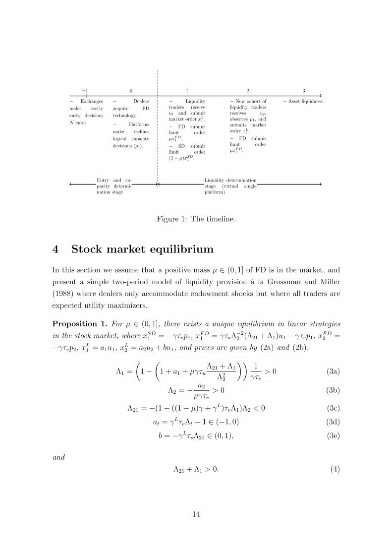
In this section we assume that a positive mass µ ∈ (0, 1] of FD is in the market, and
present a simple two-period model of liquidity provision a la Grossman and Miller
(1988) where dealers only accommodate endowment shocks but where all traders are
expected utility maximizers.
Proposition 1. For µ ∈ (0, 1], there exists a unique equilibrium in linear strategies
in the stock market, where xSD1 = −γτvp1, xFD1 = γτuΛ−22 (Λ21 + Λ1)u1− γτvp1, xFD2 =
−γτvp2, xL1 = a1u1, xL2 = a2u2 + bu1, and prices are given by (2a) and (2b),
Λ1 =
(1−
(1 + a1 + µγτu
Λ21 + Λ1
Λ22
))1
γτv> 0 (3a)
Λ2 = − a2µγτv
> 0 (3b)
Λ21 = −(1− ((1− µ)γ + γL)τvΛ1)Λ2 < 0 (3c)
at = γLτvΛt − 1 ∈ (−1, 0) (3d)
b = −γLτvΛ21 ∈ (0, 1), (3e)
and
Λ21 + Λ1 > 0. (4)
14

The coefficient Λt in (2a) and (2b) denotes the period t endowment shock’s negative
price impact, and is our (inverse) measure of liquidity:
Λt = −∂pt∂ut
. (5)
As we show in Appendix A (see (A.3), and (A.14)), a trader’s order is given by
XL1 (u1) = γL
E[v − p1|u1]Var[v − p1|u1]︸ ︷︷ ︸Speculation
− u1︸ ︷︷ ︸Hedging
XL2 (u1, u2) = γL
E[v − p2|u1, u2]Var[v − p2|u1, u2]︸ ︷︷ ︸
Speculation
− u2︸ ︷︷ ︸Hedging
.
According to (3d), a trader speculates and hedges his position to avert the risk of a
decline in the endowment value occurring when the return from speculation is low (at ∈(−1, 0)). We will refer to |at| as the trader’s “trading aggressiveness.” Additionally,
according to (3e), second period traders put a positive weight b on the first period
endowment shock. SD and FD provide liquidity, taking the other side of traders’
orders. In the first period, standard dealers earn the spread from loading at p1, and
unwinding at the liquidation price. FD, instead, also speculate on short-term returns.
Indeed,
xFD1 = γE[p2 − p1|u1]
Var[p2|u1]− γτvp1.
To interpret the above expression, suppose u1 > 0. Then, liquidity traders sell the
asset, depressing its price (see (2a)) and leading both FD and SD to provide liquidity,
taking the other side of the trade. SD hold their position until the liquidation date,
whereas FD have the opportunity to unwind it at the second round, partially unloading
their inventory risk. Anticipating this, second period traders buy the security (or
reduce their short-position), which explains the positive sign of the coefficient b in
their strategy (see (3e)). This implies that E[p2 − p1|u1] = (Λ21 + Λ1)u1 > 0, so that
FD anticipate a positive speculative short-term return from going long in the asset.
In sum, FD supply liquidity both by posting a limit order, and a contrarian market
order at the equilibrium price, to exploit the predictability of short term returns.18 In
18This is consistent with the evidence on HFT liquidity supply (Brogaard et al. (2014), and Biaiset al. (2015)), and on their ability to predict returns at a short term horizon based on market data(Harris and Saad (2014), and Menkveld (2016)).
15

view of this, Λ1 in (3a) reflects the risk compensation dealers require to hold the
portion of u1 that first period traders hedge and FD do not absorb via speculation:
Λ1 =
(1−
(1 + a1︸ ︷︷ ︸
L1 holding of u1
+ µγτuΛ21 + Λ1
Λ22︸ ︷︷ ︸
FD aggregate speculative position
))1
γτv.
In the second period, liquidity traders hedge a portion a2 of their order, which is
absorbed by a mass µ of FD, thereby explaining the expression for Λ2 in (3b).
Therefore, at both trading rounds, an increase in µ, or in dealers’ risk tolerance,
increases the risk bearing capacity of the market, leading to a higher liquidity:
Corollary 1. An increase in the proportion of FD, or in dealers’ risk tolerance
increases the liquidity of both trading rounds: ∂Λt/∂µ < 0, and ∂Λt/∂γ < 0 for
t ∈ 1, 2.
According to (2b) and (3c), due to FD short term speculation, the first period
endowment shock has a persistent impact on equilibrium prices: p2 reflects the impact
of the imbalance FD absorb in the first period, and unwind to second period traders.
Indeed, substituting (3c) in (2b), and rearranging yields: p2 = −Λ2u2 + Λ2(−µxFD1 ).
Corollary 2. First period traders hedge the endowment shock more aggressively than
second period traders: |a1| > |a2|. Furthermore, |at| and b are increasing in µ.
Comparing dealers’ strategies shows that SD in the first period trade with the same
intensity as FD in the second period. In view of the fact that in the first period the
latter provide additional liquidity by posting contrarian market orders, this implies
that Λ1 < Λ2, explaining why traders display a more aggressive hedging behavior in
the first period. The second part of the above result reflects the fact that an increase
in µ improves liquidity at both dates, but also increases the portion of the first period
endowment shock absorbed by FD. This, in turn, leads second period liquidity traders
to step up their response to u1.
Summarizing, an increase in µ has two effects: it heightens the risk bearing capacity
of the market, and it strengthens the propagation of the first period endowment shock
to the second trading round. The first effect makes the market deeper, leading traders
to step up their hedging aggressiveness. The second effect reinforces second period
traders’ speculative responsiveness. When all dealers are FD, liquidity is maximal.
16

5 Traders’ welfare, technology demand, and ex-
change equilibrium
In this section we study traders’ payoffs, derive demand and supply for technological
services, and obtain the platform competition equilibrium.
5.1 Traders’ payoffs and the liquidity externality
We measure a trader’s payoff with the certainty equivalent of his expected utility:
CEFD ≡ −γ ln(−EUFD), CESD ≡ −γ ln(−EUSD), CELt ≡ −γL ln(−EUL
t ), t ∈1, 2, where EU j, j ∈ SD,FD and EUL
t , t ∈ 1, 2, denote respectively the
unconditional expected utility of a standard dealer, a full dealer, and a first and sec-
ond period trader. The following results present explicit expressions for the certainty
equivalents.
Proposition 2. The payoffs of a SD and a FD are given by
CESD =γ
2ln
(1 +
Var[E[v − p1|p1]]Var[v − p1|p1]
)(6a)
CEFD =γ
2
(ln
(1 +
Var[E[v − p1|p1]]Var[v − p1|p1]
+Var[E[p2 − p1|p1]]
Var[p2 − p1|p1]
)(6b)
+ ln
(1 +
Var[E[v − p2|p1, p2]]Var[v − p2|p1, p2]
)).
Furthermore:
1. For all µ ∈ (0, 1], CEFD > CESD.
2. CESD and CEFD are decreasing in µ.
3. limµ→1CEFD > limµ→0CE
SD.
According to (6a) and (6b), dealers’ payoffs reflect the accuracy with which these
agents anticipate their strategies’ unit profits. A SD only trades in the first period,
and the accuracy of his unit profit forecast is given by Var[E[v− p1|p1]]/Var[v− p1|p1](the ratio of the variance explained by p1 to the variance unexplained by p1).
A FD instead trades at both rounds, supplying liquidity to first period traders,
as a SD, but also absorbing second period traders’ orders, and taking advantage of
17

short-term return predictability. Therefore, his payoff reflects the same components of
that of a SD, and also features the accuracy of the unit profit forecast from short term
speculation (Var[E[p2 − p1|p1]]/Var[p2 − p1|p1]), and second period liquidity supply
(Var[E[v − p2|p1, p2]]/Var[v − p2|p1, p2]). In sum, as FD can trade twice, benefiting
from more opportunities to speculate and share risk, they enjoy a higher expected
utility.
Substituting (3d) and (3e) in (6a) and (6b), and rearranging yields:
CESD =γ
2ln
(1 +
(1 + a1)2
(γL)2τuτv
)(7a)
CEFD =γ
2
(ln
(1 +
(1 + a1)2
(γL)2τuτv+
(1 + a1
1 + µγτuτv(µγ + γL)
)2)(7b)
+ ln
(1 +
(1 + a2)2
(γL)2τuτv
)).
An increase in µ has two offsetting effects on the above expressions for dealers’ wel-
fare. On the one hand, as it boosts market liquidity, it leads traders to hedge more,
increasing dealers’ payoffs (Corollaries 1 and 2). On the other hand, as it induces more
competition to supply liquidity it lowers them. The latter effect is stronger than the
former. Importantly, even in the extreme case in which µ = 1, a FD receives a higher
payoff than a SD in the polar case µ ≈ 0.
Proposition 3. The payoffs of first and second period traders are given by
CEL1 =
γL
2ln
(1 +
Var[E[v − p1|p1]]Var[v − p1|p1]
+ 2Cov[p1, u1]
γL
)(8a)
CEL2 =
γL
2ln
(1 +
Var[E[v − p2|p1, p2]]Var[v − p2|p1, p2]
+ (8b)
2Cov[p2, u2|p1]
γL+
Var[E[v − p2|p1]]Var[v]
−(
Cov[p2, u1]
γL
)2).
Furthermore:
1. CEL1 and CEL
2 are increasing in µ.
2. For all µ ∈ (0, 1], CEL1 > CEL
2 .
18

Similarly to SD, liquidity traders only trade once (either at the first, or at the
second round). This explains why their payoffs reflect the precision with which they
can anticipate the unit profit from their strategy (see (8a) and (8b)). Differently from
SD, these traders are however exposed to a random endowment shock. As a less
liquid market increases hedging costs, it negatively affects their payoff (Cov[p1, u1] =
−Λ1τ−1u , and Cov[p2, u2|p1] = −Λ2τ
−1u ). Finally, (8b) shows that a second period trader
benefits when the return he can anticipate based on u1 is very volatile compared to v
(Var[E[v−p2|p1]]/Var[v]), since this indicates that he can speculate on the propagated
endowment shock at favorable prices. However, a strong speculative activity reinforces
the relationship between p2 and u1, (Cov[p2, u1]2), leading a trader to hedge little of
his endowment shock u2, and keep a large exposure to the asset risk, thereby reducing
his payoff.
Substituting (3d) and (3e) in (8a) and (8b), and rearranging yields:
CEL1 =
γL
2ln
(1 +
a21 − 1
(γL)2τuτv
)(9)
CEL2 =
γL
2ln
(1 +
a22 − 1
(γL)2τuτv+b2((γL)2τuτv − 1)
(γL)4τ 2uτ2v
). (10)
An increase in the proportion of FD makes the market more liquid and leads traders
to hedge and speculate more aggressively (Corollary 2), benefiting first period traders
(Proposition 3). At the same time, it heightens the competitive pressure faced by SD,
lowering their payoffs (Proposition 2). As liquidity demand augments for both dealers’
classes, however, SD effectively receive a smaller share of a larger pie. This mitigates
the negative impact of increased competition, implying that on balance the positive
effect of the increased liquidity prevails:
Corollary 3. The positive effect of an increase in the proportion of FD on first period
traders’ payoffs is stronger than its negative effect on SD’ welfare:
∂CEL1
∂µ> −∂CE
SD
∂µ, (11)
for all µ ∈ (0, 1].
Aggregating across market participants’ welfare yields the following Gross Welfare
19

function:
GW (µ) = µCEFD + (1− µ)CESD + CEL1 + CEL
2 (12)
= µ(CEFD − CESD)︸ ︷︷ ︸Surplus earned by FD
+ CESD + CEL1 + CEL
2︸ ︷︷ ︸Welfare of other market participants
Corollary 4.
1. The welfare of market participants other than FD is increasing in µ.
2. Gross welfare is higher at µ = 1 than at µ ≈ 0.
The first part of the above result is a direct consequence of Corollary 3: as µ
increases, SD’s losses due to heightened competition are more than compensated by
traders’ gains due to higher liquidity. The second part, follows from Proposition 2
(part 3), and Proposition 3. Note that it rules out the possibility that the payoff
decline experienced by FD as µ increases, leads gross welfare to be higher at µ ≈ 0.
Therefore, a solution that favors liquidity provision by FD is also in the interest of all
market participants. Finally, we have:
Numerical Result 1. Numerical simulations show that GW (µ) is monotone in µ.
Therefore, µ = 1 is the unique maximum of the gross welfare function GW (µ).
In view of Corollary 1, gross welfare is maximal when liquidity is at its highest
level.19 Furthermore, because of monotonicity, the above market quality indicator,
becomes “measurable” welfare indexes.
19Numerical simulations where conducted using the following grid: γ, µ ∈ 0.01, 0.02, . . . , 1,τu, τv ∈ 1, 2, . . . , 10, and γL ∈ 1/√τuτv + 0.001, 1/
√τuτv + 0.101, . . . , 1, in order to satisfy (1).
20

5.2 The demand for technological services
We define the value of becoming a FD as the extra payoff that such a dealer earns
compared to a SD. According to (6a) and (6b), this is given by:
φ(µ) ≡ CEFD − CESD (13)
=γ
2
(ln
(1 +
Var[E[v − p1|p1]]Var[v − p1|p1]
+Var[E[p2 − p1|p1]]
Var[p2 − p1|p1]
)− ln
(1 +
Var[E[v − p1|p1]]Var[v − p1|p1]
)︸ ︷︷ ︸
Competition
+ ln
(1 +
Var[E[v − p2|p1, p2]]Var[v − p2|p1, p2]
)︸ ︷︷ ︸
Liquidity supply
).
FD rely on two sources of value creation: first, they compete business away from
SD, extracting a larger rent from their trades with first period traders (since they can
supply liquidity and speculate on short-term returns); second, they supply liquidity to
second period traders.
We interpret the function φ(µ) as the (inverse) demand for technological services
as it is the willingness to pay to become a FD.20
Corollary 5. The inverse demand for technological services φ(µ) is decreasing in µ.
A marginal increase in µ heightens the competition FD face among themselves,
and vis-a-vis SD. The former effect lowers the payoff of a FD. In Appendix A, we show
that the same holds also for the latter effect. Thus, an increase in the mass of FD
erodes the rents from competition, implying that φ(µ) is decreasing in µ.21
5.3 The supply of technological services and exchange equi-
librium
Depending on the industrial organization of exchanges, the supply of technological
services is either controlled by a single platform, acting as an “incumbent monopolist,”
20It formalizes in a simple manner the way in which Lewis (2014) describes Larry Tabb’s estimationof traders’ demand for the high speed, fiber optic connection that Spread laid down between NewYork and Chicago in 2009.
21Numerical simulations show that when µ, τu, and τv are sufficiently large and γ is large above γL,φ(µ) is log-convex in µ: (∂2 lnφ(µ)/∂µ2) ≥ 0. When this occurs, the price reduction correspondingto an increase in µ becomes increasingly smaller as µ increases. In these conditions, we find that forN = 2 exchanges’ best response functions can become upward sloping, differently from what happensin standard Cournot models.
21

or by N ≥ 2 venues who compete a la Cournot in technological capacities. In the
former case, the monopolist profit is given by
π(µ) = (φ(µ)− c)µ− f, (14)
where c and f , respectively denote the marginal and fixed cost of supplying a capac-
ity µ. We denote by µM the optimal capacity of the monopolist exchange: µM ∈arg maxµ∈(0,1] π(µ). In the latter case, denoting by µi and µ−i =
∑Nj 6=i µj, respectively
the capacity installed by exchange i and its rivals, and by f and c the fixed and
marginal cost incurred by an exchange to enter and supply capacity µi, an exchange
i’s profit function is given by
π(µi, µ−i) = (φ(µ)− c)µi − f. (15)
With N ≥ 2 venues we may assume that dealers are distributed uniformly across
the exchanges and that competition among exchanges proceeds in a two-stage manner.
First each exchange sets its capacity (and this determines how many dealers become FD
in the venue) and then exchanges compete in prices. This two stage game is known to
deliver Cournot outcomes under some mild conditions (Kreps and Scheinkman (1983)).
We define a symmetric Cournot equilibrium as follows:
Definition 1. A symmetric Cournot equilibrium in technological service capacities is
a set of capacities µCi ∈ (0, 1], i = 1, 2, . . . , N , such that (i) each µCi maximizes (15),
for given capacity choice of other exchanges µC−i: µCi ∈ arg maxµi π(µi, µ
C−i), (ii) µC1 =
µC2 = · · · = µCN , and (iii)∑N
i=1 µCi = µC(N).
We have the following result:
Proposition 4. There exists at least one symmetric Cournot equilibrium in techno-
logical service capacities and no asymmetric ones.
Proof. See Amir (2018), Proposition 7, and Vives (1999), Section 4.1. 2
Numerical simulations show that the equilibrium is unique and stable.22 As a
consequence, standard comparative statics results apply (see, e.g., Section 4.3 in Vives
(1999)).
22In our setup, a sufficient condition for stability (Section 4.3 in Vives (1999)) is that the elasticityof the slope of the FD inverse demand function is bounded by the number of platforms (plus one):E|µ=µC(N) ≡ −µφ′′(µ)/φ′(µ)|µ=µC(N) < 1 +N.
22

In particular, an increase in the number of exchanges leads to an increase in the
aggregate technological service capacity, and a decrease in each exchange profit:
∂µC(N)
∂N≥ 0 (16a)
∂πi(µ)
∂N
∣∣∣∣µ=µC(N)
≤ 0. (16b)
If the number of competing platforms is exogenously determined, condition (16a)
implies that spurring competition in the intermediation industry has positive effects
in terms of liquidity and gross welfare (Proposition 1 and Numerical Result 1):
Corollary 6. At a stable Cournot equilibrium, an exogenous increase in the number of
competing exchanges has a positive impact on liquidity and gross welfare: ∂Λt/∂N < 0,
∂GW/∂N > 0.
Degryse et al. (2015) study 52 Dutch stocks in 2006-2009 (listed on Euronext Am-
sterdam and trading on Chi-X, Deutsche Borse, Turquoise, BATS, Nasadaq OMX and
SIX Swiss Exchange) and find a positive relationship between market fragmentation
(in terms of a lower Herfindhal index, higher dispersion of trading volume across ex-
changes) and the consolidated liquidity of the stock. Foucault and Menkveld (2008)
also find that consolidated liquidity increased when in 2004 the LSE launched Eu-
roSETS, a new limit order market to allow Dutch brokers to trade stocks listed on
Euronext (Amsterdam).
6 Endogenous platform entry and welfare
In this section we endogenize platform entry, and study its implications for welfare
and market liquidity.23 Assuming that platforms’ technological capacities are identical
(µ = Nµi), a social planner who takes into account the costs incurred by the exchanges
23For example, according to the UK Competition Commission (2011), a platform entry fixed costcovers initial outlays to acquire the matching engine, the necessary IT architecture to operate theexchange, the contractual arrangements with connectivity partners that provide data centers to hostand operate the exchange technology, and the skilled personnel needed to operate the business. TheCommission estimated that in 2011 this roughly corresponded to £10-£20 million.
23

faces the following objective function:
P(µ,N) ≡ GW (µ)− cµ− fN (17)
= π(µi)N + ψ(µ).
Expression (17) is the sum of two components. The first component reflects the profit
generated by competing platforms, who siphon out FD surplus, and incur the costs
associated with running the exchanges: π(µi)N = ((φ(µ)− c)µi − f)N , implying that
FD surplus only contributes indirectly to the planner’s function, via platforms’ total
profit. The second component in (17) reflects the welfare of other market participants:
ψ(µ) = CESD+CEL1 +CEL
2 , and highlights the welfare effect of technological capacity
choices via the liquidity externality.24 We consider five possible outcomes:
1. Cournot with free entry (CFE). In this case, we look for a symmetric Cournot
equilibrium in µ, as in Definition 1, and impose the free entry constraint:
(φ(µC(N))− c)µC(N)
N≥ f > (φ(µC(N + 1))− c)µ
C(N + 1)
N + 1, (18)
which pins down N . We denote by µCFE, and NCFE the pair that solves the
Cournot case. Note that, given Proposition 4 and (16b), a unique Cournot
equilibrium with free entry obtains in our setup if (16b) holds and for a given N
the equilibrium is unique.
2. Structural second best (ST). In this case we posit that the planner can determine
the number of exchanges that operate in the market. As exchanges compete a la
Cournot in technological capacities, we thus look for a solution to the following
problem: maxN≥1P(µC(N), N) s. t. µC(N) is a Cournot equilibrium with
πCi (N) ≥ 0, and denote by µST , and NST the pair that solves the planner’s
problem.
3. Unrestricted Structural second best (UST). In this case we relax the non-negativity
constraint in the STR, assuming that the planner can make side-payments to ex-
changes if they do not break-even, and look for a solution to the following prob-
24Even incumbent exchanges may have to incur an entry cost to supply liquidity in the secondround. For example, faced with increasing competition from alternative trading venues, in 2009 LSEdecided to absorb Turquoise, a platform set up about a year before by nine of the world’s largestbanks. (See “LSE buys Turquoise share trading platform,” Financial Times, December 2009).
24
lem: maxN≥1P(µC(N), N) s. t. µC(N) is a Cournot equilibrium, and denote by
µUST , and NUST the pair that solves the planner’s problem.
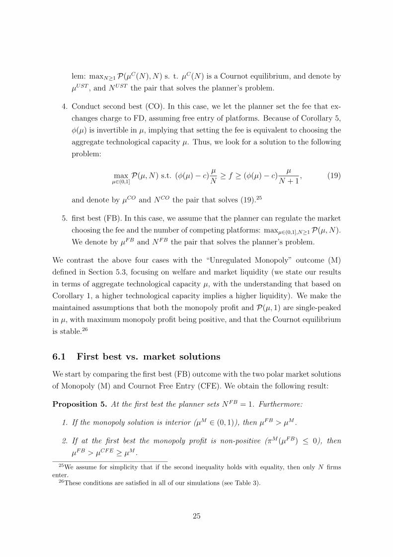
4. Conduct second best (CO). In this case, we let the planner set the fee that ex-
changes charge to FD, assuming free entry of platforms. Because of Corollary 5,
φ(µ) is invertible in µ, implying that setting the fee is equivalent to choosing the
aggregate technological capacity µ. Thus, we look for a solution to the following
problem:
maxµ∈(0,1]
P(µ,N) s.t. (φ(µ)− c) µN≥ f ≥ (φ(µ)− c) µ
N + 1, (19)
and denote by µCO and NCO the pair that solves (19).25
5. first best (FB). In this case, we assume that the planner can regulate the market
choosing the fee and the number of competing platforms: maxµ∈(0,1],N≥1P(µ,N).
We denote by µFB and NFB the pair that solves the planner’s problem.
We contrast the above four cases with the “Unregulated Monopoly” outcome (M)
defined in Section 5.3, focusing on welfare and market liquidity (we state our results
in terms of aggregate technological capacity µ, with the understanding that based on
Corollary 1, a higher technological capacity implies a higher liquidity). We make the
maintained assumptions that both the monopoly profit and P(µ, 1) are single-peaked
in µ, with maximum monopoly profit being positive, and that the Cournot equilibrium
is stable.26
6.1 First best vs. market solutions
We start by comparing the first best (FB) outcome with the two polar market solutions
of Monopoly (M) and Cournot Free Entry (CFE). We obtain the following result:
Proposition 5. At the first best the planner sets NFB = 1. Furthermore:
1. If the monopoly solution is interior (µM ∈ (0, 1)), then µFB > µM .
2. If at the first best the monopoly profit is non-positive (πM(µFB) ≤ 0), then
µFB > µCFE ≥ µM .
25We assume for simplicity that if the second inequality holds with equality, then only N firmsenter.
26These conditions are satisfied in all of our simulations (see Table 3).
25

3. Welfare comparison: PFB is larger than both PCFE and PM .
At the first best, the planner minimizes entry costs by letting a single exchange
satisfy the industry demand for technological services. If at the first best the monopoly
profit is non-positive, then aggregate capacity must be strictly larger than the one at
the Cournot Free Entry outcome since otherwise platforms would make negative prof-
its. Furthermore, the capacity supplied at the monopoly outcome can be no larger
than the one obtained with Cournot Free Entry since, under Cournot stability, in-
creased platform entry leads to increased technological service capacity. Finally, with
higher technological service capacity, and minimized fixed costs, the first best solution
is superior to either market outcome.
We can compare µFB with the capacity that obtains if the fixed cost tends to
zero, and thus the number of platforms grows unboundedly at the CFE. In this case,
platforms become price takers (PT ), and the implied aggregate capacity is implicitly
defined by: φ(µPT ) = c. Since P = (φ(µ)− c)µ+ ψ(µ), we have that P ′ = φ(µ)− c+
µφ′(µ) + ψ′(µ) and therefore:
∂P∂µ
∣∣∣∣µ=µPT
= µPTφ′(µPT ) + ψ′(µPT ), (20)
which will be positive or negative depending on whether the cost to the industry of
marginally increasing capacity (−µPTφ′(µPT )) is smaller or larger than the marginal
benefit to the other market participants (ψ′(µPT )). At µPT exchanges do not internal-
ize either effect and only in knife-edge cases we will have that µFB = µPT .27
6.2 Fee regulation
We now compare the constrained second best optimum the planner achieves with con-
duct (fee) regulation (CO) with the two polar market solutions. Under the assumption
that the monopoly profit is negative at the first best solution, which implies that at the
CO profits are exactly zero (see Lemma A.2 in Appendix A), we obtain the following
result:
Proposition 6. When the planner regulates the technological service fee, if at the first
best the monopoly profit is negative,
27Note, however, that if the welfare of other market participants is constant, then the monopolysolution implements the first best.
26

1. NCO = 1.
2. The technological service capacity supplied at the CO is lower than at the FB but
higher than at the CFE: µFB > µCO > µCFE.
3. Welfare ranking: PFB > PCO > PCFE.
Suppose that at the first best the monopoly profit is negative.28 Then with fee
regulation (CO), the aggregate technological capacity should be smaller than at the
first best since otherwise the platforms would make negative profits. As for a given
(aggregate) µ the profit of an exchange is decreasing in N , for given µ the maximum
profit obtains when N = 1 implying that NCO = 1. Furthermore, given that P is
single peaked in µ, it is optimal for µCO to be set as large as possible so that profits
are zero. Finally, with fee regulation, one platform breaks even, while at a Cournot
Free Entry (i) a single platform makes a positive profit (recall that monopoly profits
are assumed to be positive), and (ii) if more than one platform is in the market, then
platforms lose money when offering a capacity larger or equal to the one obtained with
fee regulation. In either case, µCFE < µCO, and we have: µCFE < µCO < µFB.29
Remark 1. If at the first best the monopoly profit is positive, two cases can arise.
First, we can have that (φ(µFB) − c)µFB/2 − f ≤ 0, in which case both constraints
of the Conduct second best problem are satisfied at (µCO, NCO) = (µFB, 1), and the
Conduct second best implements the first best outcome. If, on the other hand, two
platforms earn a positive profit at the first best—(φ(µFB)− c)µFB/2− f > 0—then at
a Conduct second best the planner needs to set a lower fee for technological services
compared to the one of the first best and/or allow more than one platform to enter the
market. Indeed, if NCO = 1, then by construction µCO cannot be set smaller than µFB
since this would violate the right constraint of the Conduct second best problem.
28We have numerically verified the above sufficient condition for NCO = 1, and found that in oursimulations it is always satisfied. In the reverse order of actions model, in some cases πM (µCO) > 0,but the planner still sets NCO = 1. See Table 2 for details.
29More precisely, notice that µCFE cannot be higher than µCO, as at µCO one firm makes zeroprofit. Thus, given single-peakedness of the monopoly profit, if there is either one or more than onefirm in the CFE with µCFE > µCO, profits will be negative. Similarly, it cannot be µCFE = µCO
because if NCFE = 1 then µCO = µCFE = µM , and by assumption the monopoly profit is positive;if, instead, NCFE > 1, then more than one firm shares the revenue that one firm has in the COsolution, so that its profit must be negative.
27

6.3 Entry regulation
Regulating the fee can however be complicated, as our discussion in the introduction
suggests. Thus, we now focus on the case in which the planner can only decide on the
number of competing exchanges. In the absence of regulation, a Cournot equilibrium
with free entry arises (see (18)), and we compare this outcome to the Structural second
best, in both the unrestricted and restricted cases. Evaluating the first order condition
of the planner at N = NCFE (ignoring the integer constraint) yields:
∂P(µC(N), N)
∂N
∣∣∣∣N=NCFE
= πi(µC(N), N)︸ ︷︷ ︸= 0
∣∣∣∣∣∣N=NCFE
(21)
+NCFE ∂πi(µC(N), N)
∂N︸ ︷︷ ︸Profitability depression < 0
∣∣∣∣∣∣∣∣N=NCFE
+ ψ′(µ)∂µC(N)
∂N︸ ︷︷ ︸Liquidity creation > 0
∣∣∣∣∣∣∣∣N=NCFE
.
According to (21), at a stable Cournot equilibrium, entry has two countervailing wel-
fare effects.30 The first one is a “profitability depression” effect, and captures the profit
decline associated with the demand reduction faced by each platform as a result of
entry. This effect is conducive to excessive entry, as each competing exchange does not
internalize the negative impact of its entry decision on competitors’ profits. The sec-
ond one is a “liquidity creation” effect and reflects the welfare creation of an increase
in N via the liquidity externality. This effect is conducive to insufficient entry since
each exchange does not internalize the positive impact of its entry decision on other
market participants’ payoffs.31
The above effects are related but distinct to the ones arising in a Cournot equi-
librium with free entry (Mankiw and Whinston (1986) and in the vertical oligopoly
of Ghosh and Morita (2007)).
30This is because at a stable equilibrium (16a) and (16b) hold, see section 4.3 in Vives (1999).31As clarified by condition (21), the necessary conditions for insufficient entry are: (1) that the
total technological capacity installed by entering platforms is increasing in the number of entrants–aproperty of all stable Cournot equilibria–and (2) that the gross welfare of all agents except for FD isincreasing in the total capacity of technological services that platforms supply at equilibrium–a resultthat holds in our baseline model, and that we formally prove in Corollary 4 (part 1).
28

In our setup, when we compare NCFE with NST , entry is always excessive (as
in Mankiw and Whinston (1986)); however, when NCFE is stacked against NUST , this
conclusion does not necessarily hold. More in detail, NCFE is the the largest N so
that platforms break even at a Cournot equilibrium. At the STR solution, platforms
break even too, but the planner internalizes the profitability depression effect of entry.
Thus, we have that NCFE ≥ NST . Conversely, removing the break even constraint,
the planner achieves the Unrestricted STR and, depending on which of the effects
outlined above prevails, both excessive or insufficient entry can occur:
Proposition 7. When the planner regulates entry, for stable Cournot equilibria:
1. NCFE ≥ NST , µCFE ≥ µST .
2. When the profitability depression effect is stronger than the liquidity creation
effect, NCFE ≥ NUST , µCFE ≥ µUST . Otherwise, the opposite inequalities hold.
3. Both µST and µUST are no smaller than µM .
4. Welfare ranking: PUST ≥ PST ≥ PCFE.
The first two items in the proposition reflect our previous discussion. Item 3
shows that while the technological capacity offered with free platform entry (CFE) is
higher than at the Structural second best (a natural consequence of excessive entry
with respect to the STR benchmark), when the planner relaxes the break-even con-
straint (UST), the comparison is inconclusive. Indeed, as explained above, to exploit
the positive liquidity externality, the planner may favor entry beyond the break-even
level–subsidising the loss-making platforms. Thus, while entry regulation implies that
liquidity maximization is generally at odds with welfare maximization, the two may
be aligned when the planner is ready to make up for platforms’ losses. Finally, as at
the UST the non-negativity constraint of the exchanges’ profit is relaxed, PUST ≥ PSTmust hold.
To verify the possibility of excessive or insufficient entry compared to the UST, we
run numerical simulations.32 We assume γ = 0.5, γL = 0.25, a 10% annual volatility
32We have also extended the parameter space to account for a case with “low” risk aversion (γ =25, γL = 12) which is consistent with the literature on price pressure, and recent results on thestructural estimation of risk aversion based on insurance market data (see, respectively, Hendershottand Menkveld (2014), and Cohen and Einav (2007)). In this case, we set τv = τu = 0.1 (correspondingto a 316% annual volatility for both the endowment shock and the liquidation value), f ∈ 1 ×10⁻², 1.1× 10⁻², . . . , 3.1× 10⁻², and c = 2.
29

for the endowment shock, and consider a “high” and a “low” payoff volatility scenario
(respectively, τv = 3, which corresponds to a 60% annual volatility for the liquidation
value, and τv = 25 which corresponds to a 20% annual volatility). Platform costs
are set to f ∈ 1 × 10⁻⁶, 2 × 10⁻⁶, . . . , 31 × 10−6, and c = 0.002.33 With this set
of parameters, we solve for the technological capacity and the number of platforms,
and perform robustness analysis (see Tables 2 and 3). In all simulations we obtain
πM(µFB) < 0.
Numerical Result 2. The results of our numerical simulations are as follows:
1. With high payoff volatility, entry is excessive: NCFE > NUST , and µCFE > µUST .
2. With low payoff volatility and for intermediate values of the entry cost, entry is
insufficient: NCFE < NUST and µCFE < µUST .
Furthermore, at all solutions N and µ are decreasing in f .34
Figure 2 (panels (a) and (c)) illustrates the output of two simulations in which
insufficient entry occurs. Intuitively, the combination of a high entry cost, and low
payoff volatility, work to reduce exchanges’ profit margins. A high entry cost, makes
it harder for platforms to break-even; a low payoff volatility, reduces traders’ needs
to hedge the endowment shock, lowering the rents from liquidity supply. In these
conditions, decentralizing entry decisions yields an outcome where liquidity is too low
compared to the planner’s solution. According to the figure, insufficient entry occurs.
Let us examine Figure 2(c). When f is small, both NCFE and µCFE are high.
Then, the profitability depression effect
NCFE ∂πi(µC(N), N)
∂N
∣∣∣∣N=NCFE
,
dominates the liquidity creation effect
ψ′(µ)∂µC(N)
∂N
∣∣∣∣N=NCFE
.
33Analyzing the US market, Jones (2018) argues that barriers to entry to the intermediation in-dustry are very low, a consideration that is corroborated by the current state of the market, where13 cash equity exchanges compete with over 30 ATS. This suggests that the entry cost must be low.
34Assuming γ = 0.25 < γL = 0.5 yields qualitatively similar results in the high volatility case,whereas in the low volatility case insufficient entry disappears. Additionally, with low risk aversion,we find that entry is insufficient for all levels of f , and all levels of payoff volatility.
30

In these conditions, further entry would have a limited impact on the welfare of other
market participants, consistent with the fact that in the simulations ψ(µ) is concave.
The result is thus excessive entry. As f grows, NCFE diminishes and the two effects
equilibrate. For larger values of f and smaller NCFE, encouraging entry generates
large liquidity creation benefits and there is insufficient entry at the CFE. For very
large values of f , entry is so restricted that the two forces equilibrate again since to
foster more entry is very expensive (because fN becomes very high).
6.4 Comparing all solutions
The previous sections have shown that either fee regulation (Section 6.2) or en-
try/merger policy (Section 6.3) can be used as a tool to correct platforms’ market
power, and improve aggregate welfare. The following result assesses which one of such
tools works best:
Proposition 8. Comparing solutions when πM(µFB) < 0:
1. µFB > µCO > µCFE ≥ µST ≥ µM .
2. The number of exchanges entering the market with Cournot free entry or with
entry regulation is no lower than with fee regulation (NCO = 1).
3. Welfare comparison:
PFB > PCO > PST ≥ maxPCFE,PM
≥ min
PCFE,PM
, (22a)
PFB ≥ PUST ≥ PST , (22b)
where if the FB solution is interior, then PFB > PUST .
The first two items in the proposition respectively follow from Propositions 5, 6,
and 7, and from Propositions 6, and 7.
In terms of welfare, due to Propositions 5, and 6, the first best outcome is superior
to the one achieved with fee regulation, which is in turn preferred to the monopoly
outcome. Since µST ≤ µCFE < µCO < µFB—so that we are in the increasing (in
µ) part of the planner’s objective function—and NST ≥ 1 = NCO, we have that
fee regulation is also superior to entry/merger policy (constrained by the break even
condition). In words: with entry policy the planner allows platforms to retain some
market power, to make up for the entry cost. However, if the planner can regulate
31

the fee, provided that aggregate capacity at a constrained second best solution falls
short of that implied by the first best, a superior outcome can be achieved in terms
of liquidity, which also allows to save on setup costs. Finally, entry policy (with the
break-even constraint) yields an outcome that is never inferior in terms of welfare to
the polar market solutions (CFE and M). Indeed, the latter are always available to
the planner.
The results under the assumption of Proposition 8 imply that, if unregulated, the
monopoly outcome yields lower liquidity compared to any other alternative. Further-
more, in our simulations, the planner’s objective function evaluated at µM is always
the lowest compared to the other five alternatives. Thus, both from a liquidity, and
welfare point of view the unregulated monopoly solution is the worst possible.
7 Extensions
In this section, we summarize the results of four extensions to the baseline model. In
Section 7.1, we assume that SD enter the market at the second round; in section 7.2
we suppose that a sector of “committed” SD is in the market at both rounds; in
section 7.3 we allow potential dealers to decide whether to enter the intermediation
industry, thereby endogenizing the mass of liquidity providers; finally, in section 7.4,
we consider the case in which second period traders have access to a noisy signal
about the first period endowment shock (see the online appendix for the details of
these extensions). We find in general that the results of the baseline model are robust
with one important proviso in the case of “committed” SD where entry regulation
may be welfare superior. Furthermore, we also find that for baseline parameters at the
CFE entry is always excessive both with SD in the second round, and with asymmetric
information.
7.1 SD at the second round
In this section, we assume that SD enter the market at the second round (similarly
to Huang and Yueshen (2020)). In this case (denoted RO), we find that all of the
analytical results of the baseline analysis carry through. More in detail, in relation to
the liquidity provision stage of the game, we obtain the following.
32

Proposition 9. For µ ∈ (0, 1], there exists a unique equilibrium in linear strategies
in the stock market where SD enter at the second round. Denoting by Λt, and Λ21
respectively the weight that pt assigns to ut, t ∈ 1, 2, and the one p2 assigns to u1,
compared to the baseline case, the following holds: Λ1 > Λ1, Λ1 < Λ2 < Λ2, and
|Λ21| > |Λ21|.
Thus, SD entry at the second round reduces (increases) the competitive pressure
faced by FD at the first (second) round, explaining the decrease (increase) in first (sec-
ond) period liquidity. Comparing dealers’ payoffs across the two models (maintaining
the convention of using ˜ to denote the variables obtained in the RO case), we obtain
the following result.
Proposition 10. CEFD
> CESD
, and SD have a higher payoff when entering in the
second round, whereas the result for FD is ambiguous: CESD
> CESD, and CEFD
≷
CEFD.
In the baseline model, in the first round FD supply liquidity, anticipating the
possibility to rebalance their position at the second round. This heightens the com-
petitive pressure they exert on SD compared to the model studied in this section,
explaining why CESD
> CESD. Conversely, the payoff comparison for FD is less
clear cut. Indeed, compared to the baseline model, liquidity is lower (higher) at the
first (second) round. Now the (inverse) demand for technological services is given by
φ(µ) = CEFD − CESD
, which is also decreasing in µ.
Table 3 displays the results for the simulations conducted on the baseline (OO)
and the RO models. The table shows that in the RO case, entry is excessive at all
τv. Additionally, conduct (fee) regulation yields NCO = 1 and is welfare superior to
structural (entry) regulation.
7.2 The effect of “committed” SD
In the liquidity provision model of Section 4, only FD can supply liquidity to second
period traders. This is a convenient assumption which however fails to recognize that
in actual markets liquidity provision is ensured by a multitude of market participants.
In this section we check how the introduction of a mass of “committed” SD, present in
the market at each trading round, can alter the risk-sharing properties of the market,
affecting exchanges’ technology supply, and the welfare ranking among different forms
of regulatory intervention.
33

Suppose that a mass ε of SD is unable to become FD and is in the market at
each trading round, so that in total, a mass 2ε SD are committed. Thus, at the
first round liquidity is supplied by µ FD, and a total mass 1 − µ of SD (ε of which
are committed, and 1 − ε − µ are as in the baseline model). At the second round,
instead, we have a total mass of µ FD and ε SD liquidity suppliers. In the following,
we summarize the effect of committed dealers in the model, and refer the interested
reader to the Internet Appendix for a detailed analysis. With committed dealers the
market clearing equations in Section 3.4 are replaced by: µxFD1 + (1−µ)xSD1 +xL1 = 0,
and (xFD2 − xFD1 )µ + εxSD2 + xL2 = 0, where xSD2 denotes the position of a committed
dealer at the second round. Thus, denoting by Λt, Λ21, at, and b the coefficients of
the linear equilibrium with committed dealers (which replace the corresponding price
coefficients in (2a), (2b), and traders’ strategies in Proposition 1), in the Internet
Appendix, we prove the following result:
Proposition 11. For µ ∈ [0, 1], there exists a unique equilibrium in linear strategies in
the stock market where a mass ε of SD is in the market at both rounds. At equilibrium,
the sign of the comparative statics effect of µ, as well as the ranking between liquidity
traders’ hedging aggressiveness is preserved, while
1. Λt, |at| are respectively decreasing and increasing in ε.
2. |Λ21| and b are decreasing in ε.
Committed dealers improve the risk bearing capacity of the market, increasing
its liquidity at both rounds, and leading traders to hedge a larger fraction of their
endowment shock. As second period traders face heightened competition in speculating
against the propagated endowment shock, a larger ε reduces their response to u1 (b).
To measure the impact on the welfare of market participants and the market
for technological services, we appropriately replace the equilibrium coefficients with
their tilde-ed counterparts in the expressions for the market participants’ payoffs
(see (6a), (6b), (8a), and (8b)), and compute the payoff for second period committed
dealers which, given Proposition 11, is decreasing in µ. Finally, defining the inverse
demand for technological services as the payoff difference between FD and first period
dealers: φ(µ) ≡ CEFD − CESD1 , we also obtain the following result:
Corollary 7. With committed SD:
34

1. The comparative statics effect of µ on dealers’ and traders’ payoffs, and the in-
verse demand for technological services, are as in Propositions 2, 3, and Corol-
lary 5. Furthermore, the payoff of second period committed dealers is decreasing
in µ.
2. Standard dealers’ payoffs are decreasing in ε.
Committed dealers heighten competition in the provision of liquidity, explaining the
second part of Corollary 7. Numerical simulations show that an increase in ε increases
the payoff of liquidity traders at both rounds as well as that of FD. The former effect is
in line with the improved liquidity provision enjoyed by liquidity traders. The intuition
for the latter is that besides the competitive effect, committed dealers also improve
FD ability to share risk when they retrade at the second period. This also explains
why in our simulations, the demand for technological services can be non-monotone
in ε, as shown in Figure 3.
More in detail, the demand for technological services can increase (decrease) with a
higher ε in the low (high) payoff volatility scenario. This is consistent with the fact that
an increase in τv leads first period traders to hedge a larger portion of their endowment,
increasing FD risk exposure, and thereby increasing the value of technological services
to this class of liquidity providers. Indeed, in the Internet Appendix, we show that
a1 < 0, and also that ∂a1/∂τv < 0.
0 0.2 0.4 0.6 0.8 10
0.2
0.4
0.6
0.8
1·10−2
µ
φ(µ)
γ = 0.5, γL = 0.25, τu = 100, τv = 3
ε = 0ε = 0.05
(a)
0 0.2 0.4 0.6 0.8 10
0.5
1
1.5
2·10−3
µ
φ(µ)
γ = 0.5, γL = 0.25, τu = 100, τv = 25
ε = 0ε = 0.05
(b)
Figure 3: Comparative statics effect of an increase in ε on the demand for technologicalservices.
Our simulations also confirm that as in Numerical Result 1, gross welfare: GW (µ) =
35

µ(CEFD −CESD1 ) +CESD
1 + εCESD2 +CEL
1 +CEL2 , is increasing in µ. Furthermore,
we also find that GW (µ) is increasing in ε.
We can now use the model to rank market outcomes against the different welfare
benchmarks introduced in Section 6:35
Numerical Result 3. With committed dealers, we obtain the same Numerical Result
for ε small as when ε = 0. Otherwise:
1. With high payoff volatility (τv = 3), πM(µFB) < 0, and the general ranking result
of Proposition 8 applies.
2. With low payoff volatility (τv = 25), we have that πM(µFB) > 0, and:
(a) µST = µUST , and µCO > µCFE ≥ maxµFB, µST;(b) entry regulation can yield a higher welfare than fee regulation when fixed
costs are small.
Furthermore, at all solutions N and µ are decreasing in f .
In Figure 4 we present a case in which, for a small entry cost, entry regulation
yields a higher welfare than fee regulation, a result that is at odds with Proposition 8.
The reason for this finding is as follows. The presence of committed dealers boosts
the demand for technological services, making the monopoly solution “closer” to the
first best (with ε > 0, πM(µFB) can be positive). In this case, increasing welfare
via fee regulation, requires the planner to set µ very high (much higher than at FB),
substantially depressing industry profits for mild liquidity gains. Thus, for a small
entry cost, controlling µ by choosing N can be better. Summarizing:
• When µM and µFB are far apart (πM(µFB) < 0), a very high N is needed to
increase capacity via entry, which is very expensive in terms of fixed costs (see
Figure 5, panel (a)), and it is optimal to control µ to induce N = 1.
• When µM and µFB are closer (πM(µFB) > 0), increasing welfare with CO sub-
stantially depresses industry profits for mild liquidity gains. In this case, it may
be better to control µ by choosing N (see Figure 5, panel (b)).
35We have run our numerical simulations assuming ε ∈ 0.01, 0.03, 0.05, and standard risk aversion.When ε ∈ 0.01, 0.03 and τv = 25, insufficient entry obtains for intermediate values of f , as in thebaseline model. When ε = 0.05, only excessive entry obtains.
36

µ
P(µ, 1)
µ
µFB
µM
µCO
µCFE
πM(µ)
πM(µFB)
µCO
(a)
µ
P(µ, 1)
µ
µCOµMµST
µCFEµFB
πM(µ)
πM(µFB)
(b)
Figure 5: The figure illustrates the effectiveness of alternative regulatory tools toapproach µFB. In panel (a) ε = 0, πM(µFB) < 0, and fee regulation dominates. Inpanel (b) ε > 0, and entry regulation can dominate.
7.3 Free entry into market making
In this section, we allow potential dealers to decide whether to enter the intermediation
industry prior to making the decision to become FD, thereby endogenizing the mass
of dealers who are active in the market. Importantly, this extension adds a further
equilibrium restriction to the model. Indeed, in this case we have:
1. Equilibrium conditions implied by the liquidity provision stage of the game. As-
suming that a mass of dealers µ enters the market, this condition pins down the
coefficients of the equilibrium prices at the two trading rounds Λ∗t ,Λ∗21, t ∈ 1, 2
as we have done in Section 4.
2. Equilibrium condition implied by the capacity determination stage of the game.
As done in section 5, based on the equilibrium coefficients obtained at the liquid-
ity provision stage of the game, we determine traders’ payoffs and the demand
for technological services. With this, we obtain the functional relationship µ(µ)
which yields the mass of FD as a function of the total mass of dealers who en-
tered the liquidity provision industry. Note that the specific form of this function
37

depends on the capacity competition by exchanges.
3. Equilibrium condition implied by the entry decision of dealers. Finally, replacing
the equilibrium mapping µ(µ) obtained at the previous step in SD’s payoffs, we
pin down the mass of dealers who enter the intermediation industry solving
CESD(µ(µ); µ) = K, (23)
where K represent the reservation utility of staying out of the liquidity provision
industry, and where
CESD(µ(µ); µ) =γ
2ln
(1 +
(Λ∗1)2τv
τu
). (24)
This extension is more complicated than our baseline model. Indeed, the mapping
µ(µ) (which is obtained at the second step of the algorithm described above) becomes
a crucial ingredient of equilibrium determination (i.e., the solution of (23)). Given
that the condition yielding µ(µ) is non-linear, we cannot rely on closed form solutions.
Our numerical simulations confirm the findings of Numerical Result 2:
1. With low payoff volatility (τv = 25), for intermediate values of f , entry is insuf-
ficient.
2. With high payoff volatility (τv = 3), entry is always excessive.
Additionally, in all our results NCO = 1, and fee regulation welfare dominates entry
regulation.
7.4 Asymmetric information
In this section, we assume that at the second round a liquidity trader receives an
imperfect signal about the first period endowment shock: si = u1 + εi, where εi ∼N(0, τ−1ε ), i.i.d. across traders and orthogonal to all the other random variables in the
model. With this assumption, the second period information set of a liquidity trader
becomes ΩL2 = u2, si. We solve for the equilibrium of the model, and find that
depending on the precision of second period traders’ signal, three different scenarios
arise:
1. Perfect signal. In this case, we assume that τε → ∞, and obtain the result of
the baseline model’s analysis.
38

2. Imprecise signal. In this case, we assume that 0 < τε < ∞, and find that the
equilibrium at the liquidity determination stage of the game obtains as a solution
to a 7-degree equation in Λ2 which, based on numerical analysis, admits up to
three real roots.
3. Uninformative signal. In this case, we assume that τε → 0, and find that a
unique equilibrium obtains at the liquidity determination stage of the game.
Based on our results, it is possible to show that when 0 < τε <∞, the second period
equilibrium illiquidity is straddled by the two limit cases of perfect and uninformative
second period signal. Other things equal, starting from a parametrization yielding
3 equilibria, as µ or γ increase, a unique equilibrium obtains where Λ2 tends to the
value it obtains when the signal is uninformative. Conversely, as γL, τu, or τv increase,
uniqueness obtains with Λ2 tending to the value it has in the baseline model. This
suggests that, to simplify the analysis and gauge the effect of asymmetric information,
we can concentrate on the case of an uninformative second period signal.
With this in mind, we replicate the numerical simulations of our baseline model
(i.e., using the parameter values of Table 2), assuming that second period traders
observe an uninformative signal. The result of our simulations confirm all our findings
in Numerical result 2–except for the presence of insufficient entry. Thus, when the
signal is uninformative, with the parameter values of Table 2, entry is always excessive.
Additionally, in this case too we find that NCO = 1 and that fee regulation is always
superior to entry regulation.
8 Concluding remarks
We provide a model where both supply and demand for liquidity arise endogenously,
with the former depending on exchange competition. Exchanges compete in the pro-
vision of technological services (connectivity) which improve the participation of (full)
dealers and allow them to absorb more of the net order flow, enhancing the risk bearing
capacity of the market. At equilibrium, the mass of full dealers matches the industry’s
technological service capacity. As a consequence, as exchange competition heightens,
the mass of full dealers increases, improving market liquidity and traders’ welfare. We
use the model to analyze the welfare effects of different entry regimes. A monopolistic
exchange exploits its market power, and under-supplies technological services, thereby
39

negatively affecting liquidity and welfare. Allowing competition among trading plat-
forms is beneficial for market quality and (generally) for welfare. However, the market
outcome can overprovide or underprovide technological capacity with the correspond-
ing effects on liquidity. If the regulator cannot make transfers to platforms, then entry
is never insufficient and the market never underprovides capacity when the benchmark
is regulated entry. If, on the other hand, side payments are possible, depending on
parameter values entry can also be insufficient.
The optimal second best regulatory approach turns out to depend on the magnitude
of the wedge between the technological capacity produced by a monopolistic exchange
and the one a first best planner would implement. When such a wedge is large,
approaching the first best by spurring entry involves high total fixed costs. In this case,
then, the planner limits market power by setting a fee low enough so that only one
platform can break even and provide a larger (and cheaper) capacity than the market
outcome. When, on the other hand, the wedge is small, the incremental welfare gain
achieved through fee regulation is small compared to the industry profit depression
this generates. In this case, the planner may find it better to control industry capacity
by spurring entry.
Our results suggest that exchanges’ technological capacity decisions can be an
important driver of market liquidity, adding to the usual, demand-based factors high-
lighted by the market microstructure literature (e.g., arbitrage capital, risk bearing
capacity of the market). Thus, any argument about market liquidity should take into
account the framework in which exchanges interact. Furthermore, they provide a justi-
fication for a number of recent regulatory interventions. First, the need of an “Office of
Competition Economics within [the SEC’s] Division of Economic Research and Anal-
ysis” as advocated by SEC’s commissioner Robert J. Jackson Jr., something which,
given the latest developments in the debate over the cost of technological services in
the US, seems particularly relevant.36 In this respect, our numerical results can offer
guidance as to the type of regulatory intervention. Indeed, we find that when risk-
sharing concerns are mild, platform entry is below the planner’s desired level. This
may seem surprising since with mild risk sharing concerns one would say that there is
no need for more entry. But with endogenous (platform) entry, this means that the
number of firms that enter the market is very small (low risk sharing concerns means
less business for them, because liquidity providers face a lower demand for immediacy,
which depresses their demand for technological services). In turn, this means that
36Competition: The Forgotten Fourth Pillar of the SEC’s Mission, Washington D.C., October 2018.
40

the positive liquidity externality due to an increase in the mass of FD is going to be
larger compared to profitability depression effect of new entry. In these conditions,
pro-competitive intervention is warranted precisely because the welfare gains that ac-
crue to liquidity traders more than offset the losses incurred by exchanges who end
up supplying technological services at a loss. Second, with regard to the SEC’s push
to upgrade the architecture for the consolidation and dissemination of NMS market
data.37 Through the lenses of our model such a decision corresponds to condition-
ing the technological capacity offered by exchanges, in order to increase the liquidity
creation effect. Finally, our results show the limits of the view aligning liquidity to
welfare: with excessive entry, even though the market is more liquid, a social planner
chooses to restrict competition, in this way reducing market liquidity.
Our modelling has integrated industrial organization and market microstructure
methods taking technological services as homogeneous. An extension of our approach
is to consider that exchanges offer differentiated capacities and introduce asymmetries
among exchanges. Differentiation could be both in terms of quality (e.g., speed of
connection) and horizontal attributes (e.g., lit vs. dark venues).38
37See SEC, Proposed Release No. 34-88216; File No. S7-03-20.38This would also allow to more directly contrast our results with the differentiated approach
of Pagnotta and Philippon (2018).
41

References
Abel, A. B., J. C. Eberly, and S. Panageas (2013). Optimal inattention to the stock
market with information costs and transactions costs. Econometrica 81 (4), 1455–
1481.
Aıt-Sahalia, Y. and M. Saglam (2013). High frequency traders: Taking advantage of
speed. NBER Working Paper 19531 .
Amir, R. (2018). On the Cournot and Bertrand oligopolies and the theory of super-
modular games: A survey. Handbook of Game Theory and Industrial Organization 1,
40–65.
Anand, A. and K. Venkataraman (2016). Market conditions, fragility, and the eco-
nomics of market making. Journal of Financial Economics 121 (2), 327–349.
Babus, A. and C. Parlatore (2017). Strategic fragmented markets. Working paper .
Baldauf, M. and J. Mollner (2017). Trading in fragmented markets. Working Paper .
Baron, M., J. Brogaard, B. Hagstromer, and A. Kirilenko (2019). Risk and return
in high-frequency trading. Journal of Financial and Quantitative Analysis 54 (3),
993–1024.
Biais, B., F. Declerck, and S. Moinas (2015). Who supplies liquidity, how and when?
Working paper .
Biais, B., T. Foucault, and S. Moinas (2015). Equilibrium fast trading. Journal of
Financial Economics 116, 292–313.
Brogaard, J., B. Hagstromer, L. Norden, and R. Riordan (2015, 08). Trading fast and
slow: Colocation and liquidity. The Review of Financial Studies 28 (12), 3407–3443.
Brogaard, J., T. Hendershott, and R. Riordan (2014). High frequency trading and
price discovery. Review of Financial Studies 27, 2267–2306.
Brogaard, J. A. (2010). High frequency trading and its impact on market quality.
Working Paper .
42

Budish, E., P. Cramton, and J. Shim (2015). The high-frequency trading arms race:
Frequent batch auctions as a market design response. Quarterly Journal of Eco-
nomics 139, 1547–1621.
Budish, E., R. Lee, and J. Shim (2019). Will the market fix the market? a theory of
stock exchange competition and innovation. Working Paper .
Cantillon, E. and P.-L. Yin (2011). Competition between exchanges: A research
agenda. International Journal of Industrial Organization 29 (3), 329–336.
Cespa, G. and T. Foucault (2014). Sale of price information by exchanges: Does it
promote price discovery? Management Science 60 (1), 148–165.
Chao, Y., C. Yao, and M. Ye (2019). Why discrete pricing fragments the us stock
exchanges and disperses their fee structures. Review of Financial Studies (32),
1068–1101.
Chen, D. and D. Duffie (2020). Market fragmentation. Working Paper .
Chowdhry, B. and V. Nanda (1991). Multimarket trading and market liquidity. Review
of Financial Studies 4 (3), 483–511.
Cohen, A. and L. Einav (2007). Estimating risk preferences from deductible choice.
American Economic Review 97 (3), 745–788.
Degryse, H., F. de Jong, and V. van Kervel (2015). The impact of dark trading and
visible fragmentation on market quality. Review of Finance 19, 1587–1622.
Dennert, J. (1993). Price competition between market makers. Review of Economic
Studies (60), 735–751.
Ding, S., J. Hanna, and T. Hendershott (2014). How slow is the NBBO? a comparison
with direct exchange feeds. Financial Review 49, 313–332.
Duffie, D. (2010). Presidential address: Asset price dynamics with slow-moving capital.
Journal of Finance 65 (4), 1237–1267.
Foucault, T. and A. J. Menkveld (2008). Competition for order flow and smart order
routing systems. The Journal of Finance 63 (1), 119–158.
43

Foucault, T., M. Pagano, and A. Roell (2013). Market Liquidity. Oxford University
Press.
Gabszewicz, J. and J. Thisse (1979). Price competition, quality and income disparities.
Journal of Economic Theory 20 (3), 340–359.
Ghosh, A. and H. Morita (2007). Free entry and social efficiency under vertical
oligopoly. RAND Journal of Economics 38 (3), 541–554.
Grossman, S. J. and M. H. Miller (1988). Liquidity and market structure. Journal of
Finance 43 (3), 617–37.
Harris, J. H. and M. Saad (2014). The sound of silence. The Financial Review 49,
203–230.
Hasbrouck, J. and G. Saar (2013). Low-latency trading. Journal of Financial Mar-
kets 16 (4), 646–679.
Hendershott, T. and C. M. Jones (2005). Trade-through prohibitions and market
quality. Journal of Financial Markets 8, 1–23.
Hendershott, T. and A. J. Menkveld (2014). Price pressures. Journal of Financial
Economics 114 (3), 405 – 423.
Heston, S. L., R. A. Korajczyk, and R. Sadka (2010). Intraday patterns in the cross-
section of stock returns. The Journal of Finance 65 (4), 1369–1407.
Holden, C. W. and S. Jacobsen (2014). Liquidity measurement problems in fast,
competitive markets: Expensive and cheap solutions. Journal of Finance 69 (4),
1747–1785.
Huang, S. and B. Yueshen (2020). Speed acquisition. Management Science (Forth-
coming).
Jones, C. M. (2018). Understanding the market for U.S. equity market data. Working
paper .
Kreps, D. and J. Scheinkman (1983). Quantity precommitment and bertrand compe-
tition yield cournot outcomes. Bell Journal of Economics 14 (2), 326–337.
Lewis, M. (2014). Flash Boys. London: Allen Lane.
44

Li, J. (2015). Slow price adjustment to public news in after-hours trading. Journal of
Trading 11 (3), 16–31.
Malamud, S. and M. Rostek (2017). Decentralized exchange. American Economic
Review 107, 3320–3362.
Mankiw, N. G. and M. D. Whinston (1986). Free entry and social inefficiency. RAND
Journal of Economics 17 (1), 48–58.
Manzano, C. and X. Vives (2018). Market power and welfare in asymmetric divisible
good auctions. Theoretical Economics (Forthcoming).
Menkveld, A. J. (2016). The economics of high-frequency trading: Taking stock.
Annual Review of Financial Economics 8, 1–24.
Menkveld, A. J. and M. A. Zoican (2017). Need for speed? Exchange latency and
liquidity. Review of Financial Studies 30 (4), 1188–1228.
Pagano, M. (1989). Trading volume and asset liquidity. Quarterly Journal of Eco-
nomics 104, 255–274.
Pagnotta, E. (2013). Speed, fragmentation, and asset prices. Working paper .
Pagnotta, E. and T. Philippon (2018). Competing on speed. Econometrica 86 (3),
1067–115.
Santos, T. and J. A. Scheinkman (2001). Competition among exchanges. The Quarterly
Journal of Economics 116 (3), 1027–1061.
SEC (2010). Concept release on equity market structure. Federal Register .
Shaked, A. and J. Sutton (1982). Relaxing price competition through product differ-
entiation. Review of Economic Studies 49 (1), 3–13.
UK Competition Commission (2011, November). BATS Global Markets, Inc/Chi-X
Europe Limited, merger inquiry. UK Competition Commission.
Vayanos, D. and J. Wang (2012). Liquidity and asset returns under asymmetric infor-
mation and imperfect competition. Review of Financial Studies 25 (5), 1339–1365.
Vives, X. (1999). Oligopoly Pricing: old ideas and new tools. MIT Press.
45

Vives, X. (2008). Information and learning in markets: the impact of market mi-
crostructure. Princeton University Press.
46

A Appendix
The following is a standard result (see, e.g., Vives (2008), Technical Appendix, pp.
382–383) that allows us to compute the unconditional expected utility of market par-
ticipants.
Lemma A.1. Let the n-dimensional random vector z ∼ N(0,Σ), and w = c + b′z +
z′Az, where c ∈ R, b ∈ Rn, and A is a n × n matrix. If the matrix Σ−1 + 2ρA is
positive definite, and ρ > 0, then
E[− exp−ρw] = −|Σ|−1/2|Σ−1 + 2ρA|−1/2 exp−ρ(c− ρb′(Σ−1 + 2ρA)−1b).
Proof of Proposition 1
We start by assuming that at a linear equilibrium prices are given by
p2 = −Λ2u2 + Λ21u1 (A.1a)
p1 = −Λ1u1, (A.1b)
with Λ1, Λ21, and Λ2 to be determined in equilibrium. In the second period a new mass
of liquidity traders with risk-tolerance coefficient γL > 0 enter the market. Because
of CARA and normality, the objective function of a second period liquidity trader is
given by
E[− exp−πL2 /γL|ΩL2 ] = − exp
− 1
γL
(E[πL2 |ΩL
2 ]− 1
2γLVar[πL2 |ΩL
2 ]
), (A.2)
where ΩL2 = u1, u2, and πL2 ≡ (v − p2)xL2 + u2v. Maximizing (A.2) with respect to
xL2 , yields:
XL2 (u1, u2) = γL
E[v − p2|ΩL2 ]
Var[v − p2|ΩL2 ]− Cov[v − p2, v|ΩL
2 ]
Var[v − p2|ΩL2 ]
u2. (A.3)
Using (A.1a):
E[v − p2|ΩL2 ] = Λ2u2 − Λ21u1 (A.4a)
Var[v − p2|ΩL2 ] = Cov[v − p2, v|ΩL
2 ] =1
τv. (A.4b)
A-1

Substituting (A.4a) and (A.4b) in (A.3) yields
XL2 (u1, u2) = a2u2 + bu1, (A.5)
where
a2 = γLτvΛ2 − 1 (A.6a)
b = −γLτvΛ21. (A.6b)
Consider the sequence of market clearing equations
µxFD1 + (1− µ)xSD1 + xL1 = 0 (A.7a)
µ(xFD2 − xFD1 ) + xL2 = 0. (A.7b)
Condition (A.7b) highlights the fact that since first period liquidity traders and SD
only participate at the first trading round, their positions do not change across dates.
Rearrange (A.7a) as follows:
(1− µ)xSD1 + xL1 = −µxFD1 .
Substitute the latter in (A.7b):
µxFD2 + xL2 + (1− µ)xSD1 + xL1 = 0. (A.8)
To pin down p2, we need the second period strategy of FD and the first period strategies
of SD and liquidity traders. Starting from the former, because of CARA and normality,
the expected utility of a FD is given by:
E
[− exp
− 1
γ
((p2 − p1)xFD1 + (v − p2)xFD2
)|p1, p2
]= (A.9)
= exp
− 1
γ(p2 − p1)xFD1
(− exp
− 1
γ
(E[v − p2|p1, p2]xFD2 − (xFD2 )2
2γVar[v − p2|p1, p2]
)),
For given xFD1 the above is a concave function of xFD2 . Maximizing with respect to
xFD2 yields:
XFD2 (p1, p2) = −γτvp2. (A.10)
Similarly, due to CARA and normality, in the first period a traditional market maker
A-2

maximizes
E
[− exp
− 1
γ(v − p1)xSD1
|p1]
= (A.11)
− exp
− 1
γ
(E[v − p1|p1]xSD1 −
(xSD1 )2
2γVar[v − p1|p1]
).
Hence, his strategy is given by
XSD1 (p1) = −γτvp1. (A.12)
Finally, consider a first period liquidity trader. CARA and normality imply
E[− exp−πL1 /γL] = − exp
− 1
γ
(E[πL1 |u1]−
1
2γLVar[πL1 |u1]
), (A.13)
where πL1 ≡ (v − p1)xL1 + u1v. Maximizing (A.13) with respect to xL1 , and solving for
the optimal strategy, yields
XL1 (u1) = γL
E[v − p1|u1]Var[v − p1|u1]
− Cov[v − p1, v|u1]Var[v − p1|u1]
u1. (A.14)
Using (A.1b):
E[v − p1|u1] = Λ1u1 (A.15a)
Cov[v − p1, v|u1] =1
τv. (A.15b)
Substituting the above in (A.14) yields
XL1 (u1) = a1u1, (A.16)
where
a1 = γLτvΛ1 − 1. (A.17)
Substituting (A.5), (A.10), (A.12), and (A.16) in (A.8) and solving for p2 yields
p2 = − 1− γLτvΛ2
µγτv︸ ︷︷ ︸Λ2
u2 +((1− µ)γ + γL)τvΛ1 − 1− γLτvΛ21
µγτv︸ ︷︷ ︸Λ21
u1. (A.18)
A-3

Identifying the price coefficients:
Λ2 =1
(µγ + γL)τv(A.19a)
Λ21 = Λ2
(((1− µ)γ + γL)τvΛ1 − 1
). (A.19b)
Substituting the above expressions in (A.18), and using (A.12) yields:
p2 = −Λ2u2 + Λ2
((1− µ)xSD1 + xL1
).
Consider now the first period. We start by characterizing the strategy of a FD.
Substituting (A.10) in (A.9), rearranging, and applying Lemma A.1 yields the following
expression for the first period objective function of a FD:
E[U((p2 − p1)xFD1 + (v − p2)xFD2 )|u1] = −(
1 +Var[p2|u1]
Var[v]
)−1/2× (A.20)
exp
−1
γ
(γτv2ν2 + (ν − p1)xFD1 − (xFD1 + γτvν)2
2γ
(1
Var[p2|u1]+
1
Var[v]
)−1),
where, due to (A.1a) and (A.1b)
ν ≡ E[p2|u1] = Λ21u1 (A.21a)
Var[p2|u1] =Λ2
2
τu. (A.21b)
Maximizing (A.20) with respect to xFD1 and solving for the first period strategy yields
XFD1 (p1) = γ
E[p2|u1]Var[p2|u1]
− γ(
1
Var[p2|u1]+
1
Var[v]
)p1 (A.22)
= γΛ21τu
Λ22
u1 − γτu + Λ2
2τvΛ2
2
p1.
Substituting (A.12), (A.16), and (A.22) in (A.7a) and solving for the price yields
p1 = −Λ1u1, where
Λ1 =
((1 +
µγLτuΛ2 + µγτu
)γ + γL
)−11
τv. (A.23)
A-4

The remaining equilibrium coefficients are as follows:
a1 = γLΛ1τv − 1 (A.24)
a2 = − µγ
µγ + γL(A.25)
b = −γLτvΛ21 (A.26)
Λ21 = −µγ(Λ22τv + τu)
µγτu + Λ2
Λ1 (A.27)
Var[p2|u1] =Λ2
2
τu, (A.28)
where Λ2 is given by (A.19a). An explicit expression for Λ1 can be obtained substi-
tuting (A.19a) into (A.23):
Λ1 =1 + (µγ + γL)µγτuτv
(γ + γL + (γ + 2γL)(µγ + γL)µγτuτv)τv. (A.29)
Finally, substituting (A.19a) and (A.29) in (A.27) yields
Λ21 + Λ1 =γL
τv(γµ+ γL)(γµτuτv(γ + 2γL)(γµ+ γL) + γ + γL)> 0. (A.30)
2
Proof of Corollary 1
The comparative static effect of µ and γ on Λ2 follows immediately from (A.19a). For
Λ1, differentiating (A.29) with respect to µ and γ yields:
∂Λ1
∂µ= − (2µγ + γL)γγLτu
(γ + γL + (γ + 2γL)(µγ + γL)µγτuτv)2< 0
∂Λ1
∂γ= −1 + (γ2µτuτv(γµ+ γL)2 + 2γ2µ+ 2γγLµ+ 2γγL + (γL)2)µτuτv
τv(γµτuτv(γ + 2γL)(γµ+ γL) + γ + γL)2< 0,
which proves our result. 2
Proof of Corollary 2
The first part of the corollary follows from the fact that Λ1 < Λ2. Also, since Λt is
decreasing in µ, because of (3d), |at| is increasing in µ. Finally, substituting (A.27)
A-5

in (A.26) and rearranging yields
b =µγγL(1 + (µγ + γL)2τuτv)
(µγ + γL)(γ + γL + (γ + 2γL)µγτuτv),
which is increasing in µ. 2
Proof of Proposition 2
We start by obtaining an expression for the unconditional expected utility of SD and
FD. Because of CARA and normality, a dealer’s conditional expected utility evaluated
at the optimal strategy is given by
E[U((v − p1)xSD1 )|p1] = − exp
−(E[v|p1]− p1)2
2Var[v]
= − exp
−τvΛ
21
2u21
. (A.31)
Thus, traditional dealers derive utility from the expected, long term capital gain ob-
tained supplying liquidity to first period hedgers.
EUSD ≡ E[U((v − p1)xSD1
)]= −
(1 +
Var[p1]
Var[v]
)−1/2= −
(τu1
τu1 + τvΛ21
)1/2
, (A.32)
and
CESD =γ
2ln
(1 +
Var[p1]
Var[v]
). (A.33)
Differentiating CESD with respect to µ yields:
∂CESD
∂µ=γτv2
(1 +
Var[p1]
Var[v]
)−1∂Var[p1]
∂µ(A.34)
=γτv2τu1
(1 +
Var[p1]
Var[v]
)−12Λ1
∂Λ1
∂µ< 0,
since Λ1 is decreasing in µ.
A-6
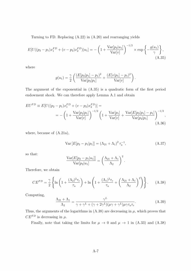
Turning to FD. Replacing (A.22) in (A.20) and rearranging yields
E[U((p2 − p1)xFD1 + (v − p2)xFD2 )|u1] = −(
1 +Var[p2|u1]
Var[v]
)−1/2× exp
−g(u1)
γ
,
(A.35)
where
g(u1) =γ
2
((E[p2|p1]− p1)2
Var[p2|p1]+
(E[v|p1]− p1)2Var[v]
).
The argument of the exponential in (A.35) is a quadratic form of the first period
endowment shock. We can therefore apply Lemma A.1 and obtain
EUFD ≡ E[U((p2 − p1)xFD1 + (v − p2)xFD2 )] =
= −(
1 +Var[p2|p1]
Var[v]
)−1/2(1 +
Var[p1]
Var[v]+
Var[E[p2|p1]− p1]Var[p2|p1]
)−1/2,
(A.36)
where, because of (A.21a),
Var [E[p2 − p1|p1]] = (Λ21 + Λ1)2 τ−1u , (A.37)
so that:Var[E[p2 − p1|u1]]
Var[p2|u1]=
(Λ21 + Λ1
Λ2
)2
.
Therefore, we obtain
CEFD =γ
2
ln
(1 +
(Λ2)2τv
τu
)+ ln
(1 +
(Λ1)2τv
τu+
(Λ21 + Λ1
Λ2
)2)
. (A.38)
Computing,Λ21 + Λ1
Λ2
=γL
γ + γL + (γ + 2γL)(µγ + γL)µγτuτv. (A.39)
Thus, the arguments of the logarithms in (A.38) are decreasing in µ, which proves that
CEFD is decreasing in µ.
Finally, note that taking the limits for µ → 0 and µ → 1 in (A.33) and (A.38)
A-7

yields
limµ→0
CESD =γ
2ln
(1 +
1
(γ + γL)2τuτv
)limµ→1
CEFD =γ
2
ln
(1 +
1
(γ + γL)2τuτv
)+ ln
(1 +
(Λ1)2τv
τu+
(Λ21 + Λ1
Λ2
)2)
,
which proves the last part of the corollary. 2
Proof of Proposition 3
Consider now first period liquidity traders. Evaluating the objective function at opti-
mum and rearranging yields
− exp
− 1
γL
(E[πL1 |u1]−
1
2γLVar[πL1 |u1]
)= − exp
−u
21
γL
(a21 − 1
2γLτv
),
where u1 ∼ N(0, τ−1u1). The argument of the exponential is a quadratic form of a
normal random variable. Therefore, applying again Lemma A.1 yields
E
[− exp
πL1γL
]= −
((γL)2τuτv
(γL)2τuτv − 1 + a21
)1/2
, (A.40)
so that
CEL1 =
γL
2ln
(1 +
a21 − 1
(γL)2τuτv
). (A.41)
Note that a higher a21 increases traders’ expected utility, and thus increases their payoff.
Next, for second period liquidity traders, substituting the optimal strategy (A.3)
in the objective function (A.2) yields
E
[− exp
−π
L2
γL
|ΩL
2
]= − exp
− 1
γL
((xL2 )2 − u22
2γLτv
)(A.42)
= − exp
− 1
γL
(xL2 u2
)( 1
2γL2 τv
(1 0
0 −1
))(xL2
u2
).
The argument of the exponential is a quadratic form of the normally distributed ran-
dom vector (xL2 u2
)∼ N
((0 0
),Σ),
A-8

where
Σ ≡(
Var[xL2 ] a2Var[u2]
a2Var[u2] Var[u2]
). (A.43)
Therefore, we can again apply Lemma A.1 to (A.42), obtaining
E
[E
[− exp
−π
L2
γL
|ΩL
2
]]= −|I + (2/γL)ΣA|−1/2, (A.44)
where
A ≡ 1
2γLτv
(1 0
0 −1
), (A.45)
Var[xL2 ] =a22 + b2
τu. (A.46)
Substituting (A.43), (A.45), and (A.46) in (A.44) and computing the certainty equiv-
alent, yields:
CEL2 =
γL
2ln
(1 +
a22 − 1
(γL)2τuτv+b2((γL)2τuτv − 1)
(γL)4τ 2uτ2v
). (A.47)
For µ = 0, b = 0 and, in view of Corollary 2, CEL1 > CEL
2 . The same condition holds
when evaluating (A.41) and (A.47) at µ = 1. As CELt is increasing in µ, we have that
for all µ ∈ (0, 1], CEL1 (µ) > CEL
2 (µ). 2
Proof of Corollary 3
We need to prove that:∂CEL
1 (µ)
∂µ> −∂CE
SD(µ)
∂µ.
Computing:
∂CEL1 (µ)
∂µ=
γLa1a′1
(γL)2τuτv − 1 + a21, (A.48)
where a′1 the partial derivative of a1 with respect to µ, and
∂CESD(µ)
∂µ=
γ(1 + a1)a′1
(γL)2τuτv + (1 + a1)2. (A.49)
First, note that the denominator in (A.49) is higher than the one in (A.48), and they
A-9

are both positive. Next, comparing the numerators in the above expressions yields:
γLa1a′1 > −γ(1 + a1)a
′1 ⇐⇒ (γLa1 + γ(1 + a1)︸ ︷︷ ︸
<0
) a′1︸︷︷︸<0
> 0,
as can be checked by substituting (A.24) in the above. Thus, the LHS of the inequality
to be proved has a higher (positive) numerator and a lower (positive) denominator
compared to the (positive) numerator and denominator of the RHS, and the inequality
follows. 2
Proof of Corollary 4
The first part of the result follows immediately from (12), and Corollary 3. Next, be-
cause of Propositions 2 and 3, GW (1) > limµ→0GW (µ), which rules out the possibility
that gross welfare is maximized at µ ≈ 0. 2
Proof of Corollary 5
Note that because of (A.39), we can write
Λ21 + Λ1
Λ2
=Λ1γ
Lτv1 + µγ(µγ + γL)τuτv
.
Therefore, substituting the expressions for dealers’ payoffs in (13), we have:
φ(µ) = CEFD − CED (A.50)
=γ
2
ln
(1 +
Λ22τvτu
)+ ln
(1 +
Λ21τvτu
K
)− ln
(1 +
Λ21τvτu
)> 0.
where K = 1+(γL/(1+µγ(µγ+γL)τuτv))2τuτv > 1, and decreasing in µ. The first term
inside curly braces in the above expression is decreasing in µ since Λ2 is decreasing in
µ. The difference between the second and third terms can be written as follows:
ln
(1 +
Λ21τvτu
K
)− ln
(1 +
Λ21τvτu
)= ln
(τu + Λ2
1τvK
τu + Λ21τv
).
Differentiating the above logarithm and rearranging yields:
τvΛ1
(τu + Λ21τvK)(τu + Λ2
1τv)
(2(K − 1)τu
∂Λ1
∂µ+ (τu + Λ2
1τu)Λ1∂K
∂µ
)< 0,
A-10

since K > 1, and both Λ1 and K are decreasing in µ. 2
We now state and prove a lemma which will be useful for some of the proofs that
follow:
Lemma A.2. πM(µFB) ≤ 0 =⇒ πM(µCO) = 0, and the converse is also true generi-
cally.
Proof of Lemma A.2
We first we prove the direction =⇒. Since πM(µFB) ≤ 0 then, given that the monopoly
profit is single-peaked, the CO constraints can only be satisfied for µ ≤ µFB. Note
that for a given (aggregate) µ, the profit of an exchange (given that it is non-negative)
is non-increasing in N ; so for a given µ, N = 1 maximizes profit. Then, given that
P(µ) is single-peaked at µFB, it is optimal for µCO to be set as large as possible with
NCO = 1, so that πM(µCO) = 0.
Next we prove the opposite direction (⇐=) generically by proving the contraposi-
tive. Suppose that at µFB the monopoly profit is positive, that is (φ(µFB)−c)µFB > f ,
then:
1. If (φ(µFB)−c)µFB/2 ≤ f , then µCO = µFB, NCO = NFB = 1 and thus πM(µCO) >
0.
2. If (φ(µFB)− c)µFB/2 > f , then given that from Proposition 5 we know that µCO ≥µM , and the monopoly profit is single peaked at µM (thus, we work in the decreasing
part of monopoly profit), we only need to examine whether it is optimal to choose
NCO > 1 and/or µCO > µFB in order to satisfy the right CO constraint.
(a) Assume that for N > 2, we do not have that (φ(µFB) − c)µFB/N = f . We
prove that it cannot be NCO > 1 with µCO ≤ µFB. Suppose by contradiction
that the latter holds. Then with µCO = µFB, the left CO constraint cannot
bind and πCO(µCO) > 0. If µCO < µFB, then the left CO constraint must bind
(and the right not): (φ(µCO)− c)µCO/NCO = f > (φ(µCO)− c)µCO/(NCO +1).
(To see this, observe that if the left did not bind, we could increase µCO to
bring it closer to µFB with both constraints still satisfied.) But then consider a
new candidate CO solution resulting from reducing NCO by one and increasing
µCO to µCO′> µCO. From the previous left CO constraint we know that
the new right CO constraint will not bind. Thus, it has to either be that
A-11

µCO′
= µFB, in which case (µCO, NCO) is rejected as a solution and we have a
contradiction, or that the new left CO constraint will bind—to see the latter,
it suffices to observe that if neither constraint binds and µCO′ 6= µFB, there
is ε > 0 small enough such that either µCO′
+ ε or µCO′ − ε increases the
planner’s function. In the case that the new left constraint binds, we have that
(φ(µCO′)− c)µCO′
/(NCO − 1) = f > (φ(µCO′)− c)µCO′
/(NCO), so µCO′< µFB
(consider a similar argument of reducing µCO′
by ε to exclude µCO′> µFB).
This case also induces P (µCO′, NCO − 1) > P (µCO, NCO), as µCO < µCO
′<
µFB. We conclude that it cannot be that NCO > 1 with some µCO < µFB.
(b) Now consider the case NCO ≥ 1 with µCO > µFB. Then the right CO con-
straint must bind (and the left not): (φ(µCO)− c)µCO/NCO > f = (φ(µCO)−c)µCO/(NCO + 1). To see this, observe that if the right did not bind, we could
reduce µCO to bring it closer to µFB with both constraints still satisfied. Thus,
πM(µCO) = (φ(µCO)− c)µCO/NCO − f > 0. 2
Proof of Proposition 5
In the first best case, for given µ, the objective function (17) is decreasing in N . Thus,
to economise on fixed costs, the planner allows a monopolistic exchange to provide
trading services, and NFB = 1. From πM(µFB) ≤ 0 it follows that:
(φ(µFB)− c)µFB ≤ f =⇒ (φ(µFB)− c)µFBN
< f, ∀N ∈ N \ 1.
We now establish the technological capacity and liquidity ranking. First, note that it
cannot be NCFE = 1 and µCFE ≥ µFB. This is because for NCFE = 1, µCFE = µM and
by assumption the monopolist makes positive profits. Thus, it will be µCFE < µFB.
Finally, by Cournot stability, µCFE ≥ µM (see also the proof of Proposition 7), with
the final implication that µFB > µCFE ≥ µM .
We now prove the welfare ranking. Since µFB > µM and P(µ, 1) is single-peaked
at µFB, it follows that PFB > PM . Also, we have that P(µ, 1) = GW (µ)− cµ− f is
single-peaked in µ at µFB, which means that GW (µ)− cµ is also single-peaked. Thus,
since µFB > µCFE we have:
PFB = GW (µFB)− cµFB − f > GW (µCFE)− cµCFE − f≥ GW (µCFE)− cµCFE − fNCFE = PCFE,
A-12

and so overall we have PFB > maxPCFE,PM
≥ min
PCFE,PM
. 2
Proof of Proposition 6
Given that the monopoly profit is negative at µFB (so that it cannot be µFB ≤ µCO),
it will be NCO = 1 and µFB > µCO so that profits are zero at the CO solution (look
also at the proof of Lemma A.2).
We now prove that µCO > µCFE. Suppose, by contradiction, that µCFE ≥ µCO.
From πM(µFB) < 0 we know that at the Conduct second best NCO = 1 and the
exchange breaks even, so given that ψ′(µ) > 0 we have:
(φ(µCFE)− c)µCFE ≤ f. (A.51)
We first deal with the case where only one firm enters at CFE, and then with the one
where NCFE > 1. At a CFE with N = 1 exchanges, we have µCFE = µM and thus
the monopolist profit is positive by assumption:
(φ(µCFE)− c)µCFE
N= (φ(µCFE)− c)µCFE = (φ(µM)− c)µM > f. (A.52)
Putting together (A.51) and (A.52) leads to a contradiction.
At a CFE with N > 1 exchanges, we need to have:
(φ(µCFE)− c)µCFE
N≥ f. (A.53)
Putting together (A.51) and (A.53) yields
f ≤ (φ(µCFE)− c)µCFE
N< (φ(µCFE)− c)µCFE ≤ f,
a contradiction. Thus, we must have µCO > µCFE.
Now, since NFB = NCO = 1 ≤ NCFE, it follows that PFB > PCO > PCFE since
µFB > µCO > µCFE and P(µ, 1) is single-peaked at µFB and, all else constant, P(µ,N)
is decreasing in N . 2
A-13

Proof of Proposition 7
Let µC(N) denote the total co-location capacity at a symmetric Cournot equilibrium
for a given number of exchanges N . The objective function of a planner that controls
entry can be written as follows:
P(µC(N), N) = Nπi(µC(N)) + ψ(µC(N)), (A.54)
where ψ(µC(N)) denotes the welfare of other market participants at the Cournot
solution:
ψ(µC(N)) = CESD(µC(N)) + CEL1 (µC(N)) + CEL
2 (µC(N)).
Consider now the derivative of the planner’s objective function with respect to N , and
evaluate it at NCFE:
∂P(µC(N), N)
∂N
∣∣∣∣N=NCFE
= πi(µC(N), N)︸ ︷︷ ︸=0
∣∣∣∣N=NCFE
(A.55)
+NCFE ∂πi(µC(N), N)
∂N︸ ︷︷ ︸<0
∣∣∣∣∣∣∣N=NCFE
+ ψ′(µC(N))∂µC(N)
∂N︸ ︷︷ ︸>0
∣∣∣∣∣∣∣N=NCFE
.
The first term on the right hand side of (A.55) is null at NCFE (modulo the integer
constraint). At a stable, symmetric Cournot equilibrium, an increase in N has a
negative impact on the profit of each exchange, and a positive impact on the aggregate
technological capacity (see, e.g., Vives (1999)). Therefore, the second and third terms
are respectively negative and positive. Given our definitions, NCFE is the largest N
such that platforms break even. NST , instead, reflects the planner’s choice of N in
Cournot equilibria that keep exchanges from making negative profits and maximizes
welfare. Hence, it can only be that
NCFE ≥ NST and µCFE ≥ µST ,
since a planner can decide to restrict entry. At a UST , the planner can make side
payments to an unprofitable exchange. This has two implications: first, the planner
A-14

can push entry beyond the level at which platforms break even, so that
NUST ≥ NST and µUST ≥ µST .
Additionally, depending on which of the two terms in (A.55) prevails, we have
∂P(µC(N), N)
∂N
∣∣∣∣N=NCFE
≷ 0 =⇒ NCFE ≶ NUST .
Finally, µC(N) ≥ µM , for N ≥ 1 because at a stable CFE the total capacity is an
increasing function of the number of platforms. A similar argument holds at both the
STR and UST, since in this case the planner picks N subject to µ being a Cournot
equilibrium
We have that PUST ≥ PST , because STR imposes an additional constraint on the
planner’s objective function compared to STR. Finally, PST ≥ PCFE, because CFE
does not account for other traders’ welfare, and the planner may choose to favour these
market participants when at the margin this creates a larger increase in GW (µ). 2
Proof of Proposition 8
From Propositions 6 and 7 we have NCO = 1, µFB > µCO > µCFE ≥ µST , PFB >
PCO > PM , and by Cournot stability µST ≥ µM . Also, we have that P(µ, 1) =
GW (µ) − cµ − f is single-peaked in µ at µFB, which means that GW (µ) − cµ is so.
Thus, since µCO > µCFE ≥ µST we have:
PCO = GW (µCO)− cµCO − f > GW (µST )− cµST − f≥ GW (µST )− cµST − fNST = PST
and so PCO > PST ≥ PCFE, where the weak inequality follows from the fact that the
CFE solution is always available in solving the STR problem. For the same reason,
PFB ≥ PUST ≥ PST ≥ PM . Thus, overall we have:
PFB > PCO > PST ≥ maxPCFE,PM
≥ min
PCFE,PM
.
Last, evaluate the derivative of welfare with respect to µ at the UST solution:
∂P(µ,N)
∂µ
∣∣∣∣(µ,N)=(µUST ,NUST )
= [φ′(µ)µ+ φ(µ)− c]|µ=µUST
A-15

The FOC of a firm i in UST reads:[φ′(µ)µ
N+ φ(µ)− c
]∣∣∣∣(µ,N)=(µUST ,NUST )
= 0.
Combining this with the above we have:
∂P(µ,N)
∂µ
∣∣∣∣(µ,N)=(µUST ,NUST )
= φ′(µ)µN − 1
N
∣∣∣∣(µ,N)=(µUST ,NUST )
< 0
so the UST solution does not maximize welfare given that the FB solution is interior
(and thus, for the UST solution to maximize welfare the derivative above should have
been zero), so it must be PFB > PUST . 2
A-16

B Market shares
Figures B.1 and B.2 replicate the ones that appear in the OECD Business and Finance
Outlook 2016 (Ch. 4, respectively Figure 4.4 and 4.6), with data that reflect the
volume for 2018. The purpose of such figures is to illustrate the degree of market
fragmentation, by showing the fraction of volume for securities that are listed on a
given exchange that is captured by the listing and competing venues. For Europe, the
lack of a public, consolidated tape, implies that one has to resort to data provided
by private institutions. Specifically, as in the OECD report, we used data provided
by “BATS for stocks listed on 12 European major exchanges” in 2018. To interpret:
for the UK, BATS data shows that about 63% of the trading in stocks listed at the
LSE takes place on that exchange, while about 22% occurs on BATS (CBOE), 9% on
Turquoise, and the remaining 6% is split between other lit and dark venues.
For the US, the exercise is facilitated by the existence of a consolidated tape, which
offers aggregate information on traded volume on- and off-exchange, and allows to use
venue “ownership” as a classification criterion (the “Off-exchange” category includes
dark-pools, crossing-networks, systemic internalizers and OTC trading).
B-1

(a) Classification of European trading venues
Trading venue Venue category
CBOE Europe CBOECBOE Europe APA CBOEInstinet Blockmatch Dark volumeITG Posit Dark volumeLiquidnet Dark volumeSIGMA X MTF Dark volumeUBS MTF Dark volumeAquis Other lit venueEquiduct Other lit venueBolsa de Madrid PrimaryEuronext PrimaryLSE Group PrimaryNasdaq OMX PrimaryOslo PrimarySIX Swiss Exchange PrimaryWiener Borse PrimaryXetra PrimaryTurquoise Turquoise
(b) Classification of US trading venues
Trading venue Venue category
EDGX Equities CBOEBZX Equities CBOEBYX Equities CBOEEDGA Equities CBOEIEX IEXNASDAQ NASDAQNASDAQ BX NASDAQNASDAQ PSX NASDAQNYSE NYSENYSE Arca NYSENYSE Chicago NYSENYSE American NYSENYSE National NYSENASDAQ TRF Carteret Off-exchangeNYSE TRF Off-exchangeNASDAQ TRF Chicago Off-exchange
Table 1: Trading venues classification for Figures B.1 and B.2.
Initial parametrizationAlternative parameter valuesc γ γL
c = 0.002, γ = 0.5, γL = 0.25, τu = 100, τv = 25 0.001 0.45, 0.35, 0.3, 0.25 0.15c = 0.002, γ = 0.5, γL = 0.25, τu = 100, τv = 3 0.003 0.45, 0.35, 0.3, 0.25 0.15c = 2, γ = 25, γL = 12, τu = 0.1, τv = 0.1 2.5 22.5, 17.5, 15, 12.5 18
Table 2: Parametrizations used in the simulations. The third row of the table refersto a parametric extension that we have employed in the simulation of the baseline caseand the one where SD enter at the second round.
B-1

0 0.5 1 1.5 2 2.5 3
·10−6
0.5
1
1.5
·10−2
f
µCFE
µCO
µST
µUST
µM
µFB
0 0.5 1 1.5 2 2.5 3
·10−6
0
2
4
6
8
10
12
f
NCFE
NCO
NST
NUST
c = 0.002, γ = 0.5, γL = 0.25, τu = 100, τv = 25, ε = 0
(a)
0 0.5 1 1.5 2 2.5 3
·10−6
0.2
0.4
0.6
0.8
f
µCFE
µCO
µST
µUST
µM
µFB
0 0.5 1 1.5 2 2.5 3
·10−6
0
50
100
150
f
NCFE
NCO
NST
NUST
c = 0.002, γ = 0.5, γL = 0.25, τu = 100, τv = 3, ε = 0
(b)
0 0.5 1 1.5 2 2.5 3
·10−6
2
4
6
8
·10−3
f
µCFE
µCO
µST
µUST
µM
µFB
0 0.5 1 1.5 2 2.5 3
·10−6
0
5
10
f
NCFE
NCO
NST
NUST
c = 0.003, γ = 0.5, γL = 0.25, τu = 100, τv = 25, ε = 0
(c)
0 0.5 1 1.5 2 2.5 3
·10−6
0.2
0.3
0.4
0.5
0.6
f
µCFE
µCO
µST
µUST
µM
µFB
0 0.5 1 1.5 2 2.5 3
·10−6
0
50
100
f
NCFE
NCO
NST
NUST
c = 0.003, γ = 0.5, γL = 0.25, τu = 100, τv = 3
(d)
Figure 2: Panels (a) and (c) illustrate two cases in which insufficient entry occurs. InPanel (b) and (d), entry is always excessive.
B-2
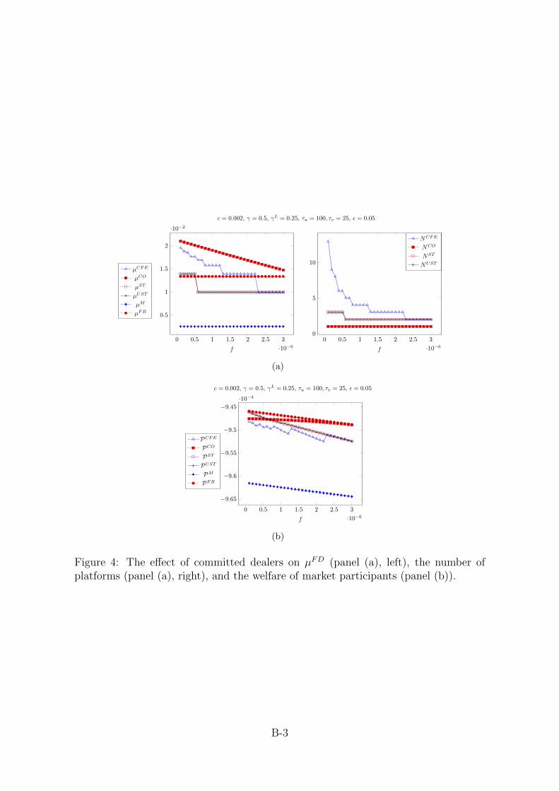
0 0.5 1 1.5 2 2.5 3
·10−6
0.5
1
1.5
2
·10−2
f
µCFE
µCO
µST
µUST
µM
µFB
0 0.5 1 1.5 2 2.5 3
·10−6
0
5
10
f
NCFE
NCO
NST
NUST
c = 0.002, γ = 0.5, γL = 0.25, τu = 100, τv = 25, ε = 0.05
(a)
0 0.5 1 1.5 2 2.5 3
·10−6
−9.65
−9.6
−9.55
−9.5
−9.45·10−4
f
PCFE
PCO
PST
PUST
PM
PFB
c = 0.002, γ = 0.5, γL = 0.25, τu = 100, τv = 25, ε = 0.05
(b)
Figure 4: The effect of committed dealers on µFD (panel (a), left), the number ofplatforms (panel (a), right), and the welfare of market participants (panel (b)).
B-3

0%
10%
20%
30%
40%
50%
60%
70%
80%
90%
100%
London Frankfurt Paris Zurich Milan Amsterdam Madrid Stockholm Copenhagen Brussels Helsinki Oslo
Primary CBOE Turquoise Other lit venue Dark volume
Figure B.1: Market shares among trading venues in Europe in 2018. Source: CBOEGlobal Markets, own calculations (See Table 1 (Panel (a)) for venues’ classification).
Figure B.2: Market shares among trading venues in the US in 2018. Source: CBOEGlobal Markets, own calculations (See Table 1 (Panel (b)) for venues’ classification).
B-4

Res
ult
Ord
erof
acti
onP
aram
etri
zati
on
NCFE<NUST
OO
c=
0.00
2,γ∈0.4
5,0.
5,γL
=0.
25,τ u
=10
0,τ v
=25
c=
2,γ∈2
5,22.5,1
7.5,
15,1
2.5
,γL
=12
,τ u
=0.
1,τ v
=0.
1
c=
2,γ
=25
,γL
=18
,τ u
=0.
1,τ v
=0.
1
RO
c=
2,γ∈2
5,22.5,1
7.5,
15,1
2.5
,γL
=12
,τ u
=0.
1,τ v
=0.
1
c=
2,γ
=25
,γL
=18
,τ u
=0.
1,τ v
=0.
1
c=
2.5,γ
=25
,γL
=12
,τ u
=0.
1,τ v
=0.
1
NCFE<NUST−
1O
Oc
=2,γ∈2
5,22.5,1
7.5,
15,1
2.5
,γL
=12
,τ u
=0.
1,τ v
=0.
1
RO
c=
2,γ∈1
7.5,
15,1
2.5
,γL
=12
,τ u
=0.
1,τ v
=0.
1
πM( µFB
) >0,µCO>µCFE>µFB
RO
c=
0.0
02,γ
=0.5
,γL
=0.2
5,τ u
=10
0,τ v∈3,2
5an
dal
lsh
ifts
arou
nd
pre
sente
din
Tab
le2
πM
(µFB
)≤
0O
O(γ,γL,τu,τv,c,f
):γ,γL∈1,2,...,2
5,τu,τv∈0.1,0.2,...,1
0,
c∈0.0
1,0.0
2,...,
0.5,f∈0.0
01,0.0
02,...,0.1
NCO
=1
OO
Th
eth
ree
par
amet
riza
tion
sin
Tab
le2.
RO
Sin
gle-
pea
ked
nes
sofP
(µ,1
)an
dπ
(µ)
OO
Th
eth
ree
par
amet
riza
tion
sin
Tab
le2.
RO
Tab
le3:
Cas
esw
her
eva
riou
sphen
omen
aar
eob
serv
ed.
OO
and
RO
refe
rto
the
orig
inal
and
reve
rse
order
ofac
tion
model
s,re
spec
tive
ly.
B-5