Exchange bias of polycrystalline antiferromagnets with perfectly compensated interface

D. Suess, M. Kirschner, T. Schrefl, J. Fidler

1Institute of Solid State Physics, Vienna University of Technology, Wiedner Hauptstr. 8-10, A-1040 Vienna, Austria

R. L. Stamps and J.-V. Kim

School of Physics, University of Western Australia, 35 Stirling Highway, Crawley WA 6009, Australia

ABSTRACT

A mechanism for exchange bias and training for antiferromagnet/ferromagnet bilayers with fully

compensated interfaces is proposed. In this model, the bias shift and coercivity are controlled by

domain wall formation between exchange coupled grains in the antiferromagnet. A finite element

micromagnetic calculation is used to show that a weak exchange interaction between randomly ori-

ented antiferromagnetic grains and spin flop coupling at a perfectly compensated interface are suffi-

cient to create shifted hysteresis loops characteristic of exchange bias. Unlike previous partial wall

models, the energy associated with the unidirectional anisotropy is stored in lateral domain walls

located between antiferromagnetic grains. We also show that the mechanism leads naturally to a

training effect during magnetization loop cycling.

PACS: 75.50.Ee; 75.70.Kw; 75.60.Jk; 75.40.Mg

KEYWORDS: exchange bias, compensated interface, antiferromagnetic domains, micromagnetics

Contact author: Dieter Suess

Institute of Solid State Physics

Vienna University of Technology

Wiedner Hauptstr. 8-10

A-1040 Vienna

E-mail: suess@magnet.atp.tuwien.ac.at

FAX: +43-1-58801-13798

page 2

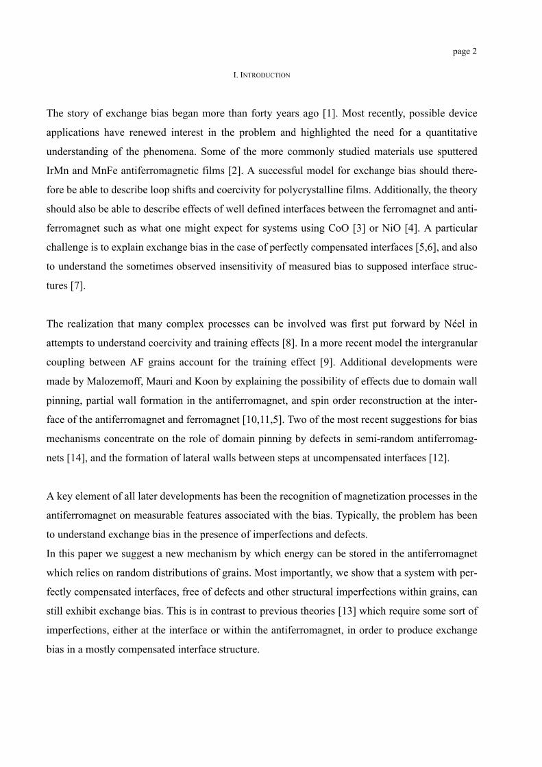
I. INTRODUCTION

The story of exchange bias began more than forty years ago [1]. Most recently, possible device

applications have renewed interest in the problem and highlighted the need for a quantitative

understanding of the phenomena. Some of the more commonly studied materials use sputtered

IrMn and MnFe antiferromagnetic films [2]. A successful model for exchange bias should there-

fore be able to describe loop shifts and coercivity for polycrystalline films. Additionally, the theory

should also be able to describe effects of well defined interfaces between the ferromagnet and anti-

ferromagnet such as what one might expect for systems using CoO [3] or NiO [4]. A particular

challenge is to explain exchange bias in the case of perfectly compensated interfaces [5,6], and also

to understand the sometimes observed insensitivity of measured bias to supposed interface struc-

tures [7].

The realization that many complex processes can be involved was first put forward by Néel in

attempts to understand coercivity and training effects [8]. In a more recent model the intergranular

coupling between AF grains account for the training effect [9]. Additional developments were

made by Malozemoff, Mauri and Koon by explaining the possibility of effects due to domain wall

pinning, partial wall formation in the antiferromagnet, and spin order reconstruction at the inter-

face of the antiferromagnet and ferromagnet [10,11,5]. Two of the most recent suggestions for bias

mechanisms concentrate on the role of domain pinning by defects in semi-random antiferromag-

nets [14], and the formation of lateral walls between steps at uncompensated interfaces [12].

A key element of all later developments has been the recognition of magnetization processes in the

antiferromagnet on measurable features associated with the bias. Typically, the problem has been

to understand exchange bias in the presence of imperfections and defects.

In this paper we suggest a new mechanism by which energy can be stored in the antiferromagnet

which relies on random distributions of grains. Most importantly, we show that a system with per-

fectly compensated interfaces, free of defects and other structural imperfections within grains, can

still exhibit exchange bias. This is in contrast to previous theories [13] which require some sort of

imperfections, either at the interface or within the antiferromagnet, in order to produce exchange

bias in a mostly compensated interface structure.

page 3

Consider a ferromagnetic film exchange coupled to an ensemble of antiferromagnetic grains. Even

if the interface is assumed to be everywhere perfectly compensated, spin flop canting at the interface

can provide a small net magnetic moment to which the ferromagnet can couple. The spin flop con-

figuration is not stable without certain effective anisotropies, and will not lead to exchange bias for

realistic antiferromagnet material parameters. The reason is that during magnetization reversal, a

canted antiferromagnetic interface is unstable to out of plane fluctuations and can nucleate a reversal

of the antiferromagnet sublattices [6]. This can result in coercivity, but does not produce a shifted

hysteresis loop for the ferromagnet.

An interesting possibility appears if the uniaxial anisotropy axes of the individual antiferromagnetic

grains are randomly oriented. The significance of a distribution of uniaxial directions lies in the dif-

ferent effects reversal of the ferromagnet produces for different axis orientations. To appreciate this,

consider how a canted antiferromagnetic grain exchange coupled to a single domain ferromagnetic

grain reverses with the ferromagnet. The spin flop configuration expected for a compensated inter-

face can be represented schematically as shown in Fig.1. The thick arrow represents the ferromagnet

spins, and the arrows labelled a and b are the two antiferromagnet sublattices. A spin flop configu-

ration is shown in (a) where the dotted line is the orientation of the antiferromagnet uniaxial axis.

The anisotropy energy involved in the spin flop configuration is given by

, where K1 is the anisotropy energy and M is the sublattice magnetiza-

tion. az and bz are the projection of the magnetization of sublattice A and B on the easy axis, respec-

tively.

Suppose now that the interlayer exchange coupling is comparable in magnitude to the antiferromag-

netic exchange and anisotropies such that the spin flop configuration can rotate rigidly when a field

is applied. Reversal of the ferromagnet under application of a small applied field will cause both

sublattice spins to rotate with the ferromagnet. Rotations about the anisotropy axis of the antiferro-

magnet leave Eani unchanged and are reversible. Rotations about any other direction change Eani

and can involve irreversible changes in the magnetic configuration. Reversal of the ferromagnet and

spin flopped antiferromagnet with a random distribution of antiferromagnet uniaxial anisotropy

axes therefore involves both reversible and irreversible changes in the antiferromagnet.

Eani K1 az2 bz

2+( )/M2–=

page 4

If the antiferromagnet grains do not interact via exchange coupling across intergrain boundaries, co-

ercivity will be observed in the antiferromagnet in proportion to the fraction of irreversibly switched

grains, but there will not be a shifted hysteresis. Shifted hysteresis will appear only if the energy of

the system changes upon reversal. This can occur in the random axis spin flop model described

above if interactions between antiferromagnet grains exist. The reason can be seen using the nota-

tion defined in Fig. 1 (b). The vector l is the projected sum of the sublattice magnetizations on the

anisotropy axis of a grain, and the vector t is the component of the sublattice magnetization sum

perpendicular to the anisotropy axis.

Suppose two grains have antiferromagnet anisotropy axes aligned as shown in Fig. 1 (c) with cor-

responding projections l1, t1 and l2 and t2. Consider what happens if the ferromagnet reverses by

rotating around l1. The angle between t1 and t2 does not change upon reversal of the ferromagnet,

but the angle between l1 and l2 does. If the angle between l1 and l2 is not zero or 90o, the change in

angle will involve a change in intergranular exchange energy. This means that the magnitude of the

intergranular exchange energy can change upon reversal of the ferromagnet depending on the rela-

tive orientation of anisotropy axes for adjacent grains.

During reversal in a planar geometry where the ferromagnet is constrained by demagnetizing fields

to lie in the film plane, the spins in antiferromagnetic grains with axes nearly perpendicular to the

interface will not be strongly affected by the changing orientation of the ferromagnet. This is in con-

trast to the spins in antiferromagnetic grains with axes parallel to the interface in which it is not pos-

sible for the spin flop configuration to follow the ferromagnet without irreversible switching. The

energy difference resulting from intergranular coupling leads to an additional torque acting on the

ferromagnet that appears as a bias field resulting in a shifted hysteresis.

In order to explore this idea, we have performed a finite element micromagnetic calculation of a fer-

romagnet/antiferromagnet bilayer. Technical details of the calculation are given elsewhere [15], and

the essential feature is that a two lattice approach was developed in which the spin directions on a

length scale of the exchange length are combined to a magnetization direction on one finite element.

The strayfield is taken in account using a hybrid finite element boundary element method. The finite

element calculation for antiferromagnet/ferromagnet structures results in the same spin flop cou-

pling as obtained by micromagnetic calculations on an atomistic length scale [5]. In the remainder

page 5

of the present paper we discuss a simplified version of this model suitable for examining very large

ensembles of grains. The results agree well with those of the finite element model but highlights

most clearly the crucial role of randomness in the antiferromagnet necessary to generate exchange

bias. We also show that this intrinsic dependence on randomness naturally provides a mechanism

for training effects.

Before discussing the model and results, note should be made of two previous recent proposed

mechanisms. Morosov and Sigov [12] proposed a model in which exchange bias appears due to a

magnetic configuration generated between steps at an uncompensated interface. The grain model

discussed here involves the formation of narrow domain walls between grains, along the interface.

Our mechanism involves lateral walls of a sort, but applies to compensated interfaces, free of geo-

metrical imperfections.

The second mechanism is called the domain state model, and has been proposed by Nowak et al.

[14]. This model describes an exchange bias due to domain wall pinning by random defects. A net

moment caused by uncompensated spins provides coupling across the interface, and the authors

find a bias shift for directions parallel to the antiferromagnetic anisotropy axis for spins in a single

crystal lattice. Our model assumes no defects except for grain boundaries, and coupling is due to

spin flop at a perfect compensated interface. The antiferromagnetic film is not a single crystal but

instead a collection of small crystallites with randomly oriented axes. In our model the energy

associated with exchange bias is stored in AF domain walls. The interface energy is merely to pro-

vide coupling to the antiferromagnetic domains, and otherwise plays no role in the formation of

bias. In contrast, the domain state model the interface energy is argued to play a dominate role in

the formation of bias.

II. INTERACTING GRAIN MODEL

The model is described by a single grain energy which is composed of anisotropy, Zeeman, and

intergrain exchange energy terms. We assume a polycrystalline antiferromagnetic film of thickness

tAF coupled to a polycrystalline ferromagnetic film of thickness tF. For small grain size and low

intergrain exchange coupling the magnetization within a grain remains nearly uniform. This means

for example that a partial wall cannot form in a grain and there is a maximum thickness for which

page 6

the model applies. We assume a compensated interface and therefore introduce a 90° coupling

between the AF layer and F layer following suggestions by Stiles and McMichael [16] and as

derived by Stamps [17]. The total energy per grain j is

(1)

The sum over i is over the nearest neighbor grains. S is the total spin quantum number, l the grain

diameter. JF and JAF denote the exchange integral across ferromagnetic grains and antiferromag-

netic grains, respectively. JAF-F describes the total effective exchange interaction at the compen-

sated interface. The exchange energies depend on the number of spins per area at the interface, nI,

at the ferromagnetic grain boundary, nF, and at the antiferromagnetic grain boundary, nAF. The

geometry used in defining Eq. (1) is shown in Fig. 2. and denote the unit vector of the

spin direction in the grain j of the antiferromagnet and ferromagnet, respectively. The third term in

Eq. (1) describes the 90o coupling associated with a canted spin flop state formed at a compensated

interface. The antiferromagnetic spins are not fully antiparallel near the interface. This canted state

is strongly localized to the interface. In the bulk of the antiferromagnet the spins of the different

sublattices are antiparallel for the typical fields applied in applications. This means that as long as

the applied field is not larger than the antiferromagnetic exchange, as is the case in most experi-

ments, magnetic surface and volume charges cancel in the antiferromagnet. Any remaining contri-

butions to magnetostatic energy for individual magnetic sublattices in the antiferromagnet can be

taken into account through the anisotropy constant, K1. Shape effects for the ferromagnetic film are

approximated with the fifth term in Eq. (1) by assuming an in plane anisotropy energy proportional

to the square of the magnetization. In this term, kF is a unit vector pointing perpendicular to the

film plane. The antiferromagnet has a uniaxial anisotropy of strength K1 and the easy axis direction

is assigned randomly for every grain. Finally, we assume that an external static magnetic field

Ej J– FS2nFtFluFj uF

i JAFS2nAFtAFluAFj uAF

i–[ ]i 1=

nN

∑ JAF-FS2nI uAFj uF

j( )2 l2–=

K1 kAFj uAF

j( )2tAFl2 Js2 µ0⁄( ) kF

j uFj( )2tFl2+– JsHuF

j tFl2

–

uAFj uF

j

kAF

page 7

H only acts on the ferromagnet. This energy is given by the sixth term in Eq. (1) where Js is the

magnitude of the spontaneous magnetization.

Hysteresis loop calculations are made by first initializing the system by simulating field cooling

and then following the evolution of the magnetization with changing the applied magnetic field.

An equilibrium configuration is found at each magnetic field value. The equilibrium state is

obtained by the numerical integration of the Landau-Lifshitz-Gilbert [18] equation using effective

fields determined from the energy in Eq. (1). The field acting on the antiferromagnet is found using

, (2)

where is the total sublattice moment of the antiferromagnetic component of grain j. A sim-

ilar expression is used to calculate the effective field acting on the ferromagnet. We assume the

system to be in equilibrium if the change of the magnetization, du/dt, is smaller than 10-4µ0 on

every node. A backward differentiation method [19] is used to integrate the LLG equation numeri-

cally.

III. BIAS FIELDS AND TRAINING

For the following simulations parameters are chosen to approximate materials used in GMR read-

heads, such as IrMn. In the antiferromagnet, K1 = 1 x 105 J/m3, JAF = 0.023 meV. The antiferromag-

netic layer consists of 60x 60 rectangular grains with basal plane area 10x10 nm2. The grain struc-

ture in the ferromagnet is the same as in the antiferromagnet. The thickness of the ferromagnet is

10nm in all cases. The intergrain interaction between ferromagnetic grains is JF = 0.45 meV. The

coupling between the ferromagnet and antiferromagnet is completely compensated, with the effec-

tive interface exchange, JAF-F = -0.45 meV.

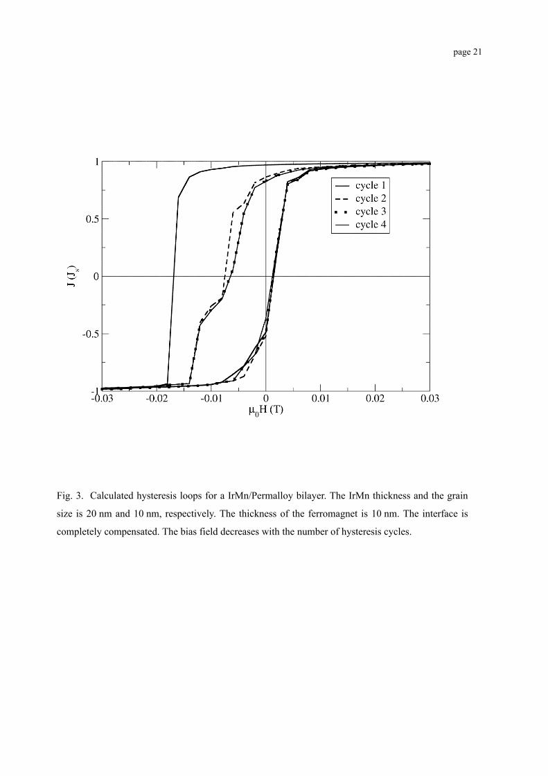
Calculated hysteresis loops for a antiferromagnet thickness of 20nm are shown in Fig. 3. To initial-

ize the system, field cooling is simulated using a Metropolis Monte Carlo algorithm. The ferromag-

net direction is fixed, and the magnetization of the antiferromagnet is set randomly. Three different

trial steps [20] are used to efficiently sample the phase space of spin configurations. Each Monte

Carlo step begins by randomly choosing an antiferromagnetic grain and making the following three

Heff AF,j 1

JstAFl2-----------------

uAFj∂

∂Etot–=

JstAFl2

page 8

tests, each chosen according to a Metropolis Monte Carlo algorithm: A new magnetization direction

is randomly chosen (1) within a cone of an angle of 3° such that the symmetry axis of the cone is

parallel to the old magnetization direction; (2) within any orientation on a sphere; and (3) as a simple

reversal. We start the cooling process at a temperature of T = 800 K and decrease the temperature to

T = 0 in steps of ∆T = 25 K. At each temperature we scan the lattice 2000 times.

The initial field strength is µ0H=0.1T and is decreased in steps of µ0∆H = -0.002 T. In order to in-

vestigate the training effect several hysteresis cycles are calculated. Cycle 1 of the loops in Fig. 3.

is calculated starting from the field cooled state as initial configuration and has a bias field of

(µ0Hb= 7.7mT). The next cycle (cycle 2) shows a reduction of the bias field by about 65%.

Because the hysteresis loops are obtained at zero temperature there are no effects due to thermal

fluctuations. Training appears only because the domain configuration in the antiferromagnet is

strongly dependent on a history created by irreversible switching of antiferromagnets in the ensem-

ble of grains. The ferromagnet orientation does not change during cooling. After cooling, the only

equilibration process available to the antiferromagnet appears through changes in the state of the

ferromagnet. Only a fraction of the antiferromagnet grains reverse during each cycle, but some

grains do not. The relative magnitude of these two populations in a steady state configuration is

essentially a self consistent solution that minimizes the total energy of the many grain ensemble. It

is not necessarily the lowest energy solution and is sensitive to the initial conditions, size of the

applied field step used, and applied field limits. In our simulations, a steady state equilibrium

appeared after about four cycles.

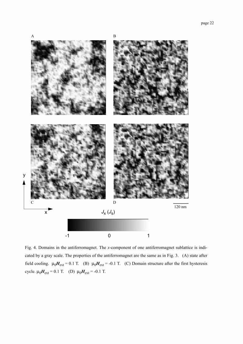
The approach to a steady state solution is illustrated in Fig. 4. In this figure, domain configurations

at different points along the magnetization curve are shown after field cooling using gray scales to

indicate the orientation of one antiferromagnet sublattice. The magnetization of one sublattice of the

antiferromagnet parallel to the x-axis is indicated by a gray scale (left = black, right = white). The

external field in (A) is µ0Hext=0.1T. Note the formation of large domains with diameters of several

hundred nanometers. This is consistent with the thermal annealing and cooling at high field which

favours formation of uniform domains with a minimum of domain boundary walls.

page 9

The domain configuration in the antiferromagnet at µ0Hext=-0.1T after the reversal of the ferro-

magnet is shown in Fig. 4 (B). The large domains seen in (A) break up into a number of smaller

domains. This represents a higher energy configuration than in (A) because of the increase in

energy involved in creating domain walls.

The domain configuration is shown in (C) for the system after it is brought back to the field

µ0Hext=0.1T as the first loop is completed. The domains are larger than in (B), corresponding to a

lower total energy since the number of domain walls is reduced. Note however that a number of

antiferromagnetic grains did not reverse back to their original orientation just after field cooling.

Consequently the domains in the antiferromagnet are somewhat smaller on average than in (A),

and the total energy is also higher.

It is interesting that even though this is a zero temperature process, the original field cooled config-

uration will never again appear as the field is cycled further. The reversed ferromagnet configura-

tion for the second cycle µ0Hext=-0.1T point is shown in (D). The steady state configuration is not

yet achieved and the high energy state of (D) is different from that in the first cycle shown in (B).

The origin of this athermal behavior is in the nature of how the antiferromagnet orders. As pointed

out above, the antiferromagnet is affected not by the applied field directly, but instead through

exchange coupling to the ferromagnet. During the demagnetization and magnetization branches of

a cycle, the ferromagnet locally aligns in such a way as to minimize competing energies due to the

applied field and exchange energies through coupling with the antiferromagnet. The random

anisotropy axes of the antiferromagnet force the ferromagnet to adopt an equilibrium configuration

that varies spatially. From the point of view of the antiferromagnet, the orientation of the ferromag-

net varies spatially and creates a random field whose exact configuration depends on the applied

field strength. In this way the antiferromagnet responds to a series of different spatially distributed

random fields during a magnetization loop cycle.

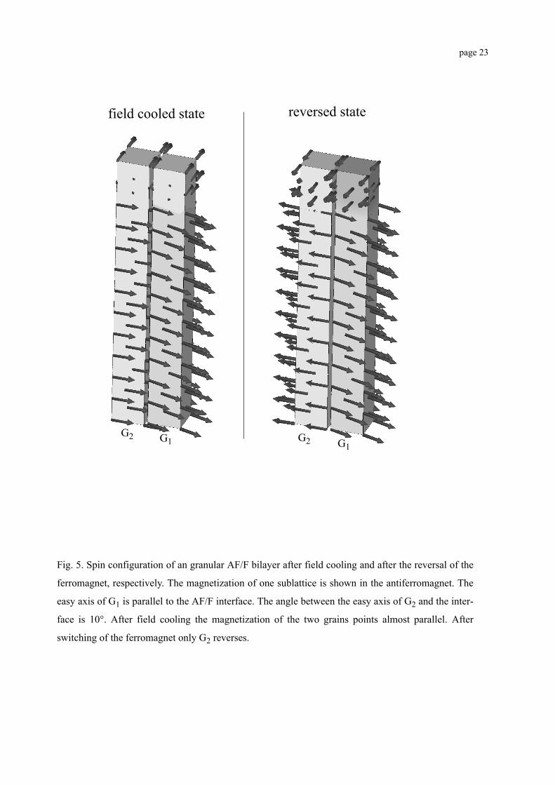
The exchange bias hysteresis loop shift persists after cycling and is due to the fraction of grains

that remain fixed during the magnetization process, and intergranular exchange energy incurred

with adjacent grains that reverse. An example is shown in Fig. 5 for two grains. Arrows in the anti-

ferromagnet identify one sublattice only for simplicity. After field cooling the ferromagnet and this

sublattice of the antiferromagnet are aligned corresponding to a low energy state. Upon reversal,

page 10

the grain on the right (G1) remains fixed, but the grain on the left (G2) switches. G1 did not switch

because its axis is aligned with a component normal to the film plane. The easy axis in G2 is paral-

lel to the film plane that allows a 180° rotation of the antiferromagnet magnetization as the ferro-

magnet is reversed. Because of the antiparallel orientation of the spins in the reversed state this

state has a larger intergranular exchange energy than the field cooled state.

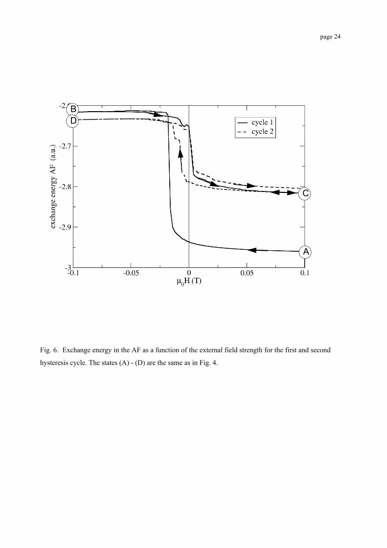
The energy involved in forming pinned domain walls between antiferromagnetic grains is respon-

sible for the exchange bias shift. After the steady state is reached, this energy can be recovered by

untwisting the wall. The intergranular energy is plotted in Fig. 6 as a function of the applied field

for several cycles. The minimum energy is always in the field cooling direction regardless of the

cycle, and takes the smallest value directly after field cooling and before cycling. The total energy

increases when the ferromagnet switches as discussed above.

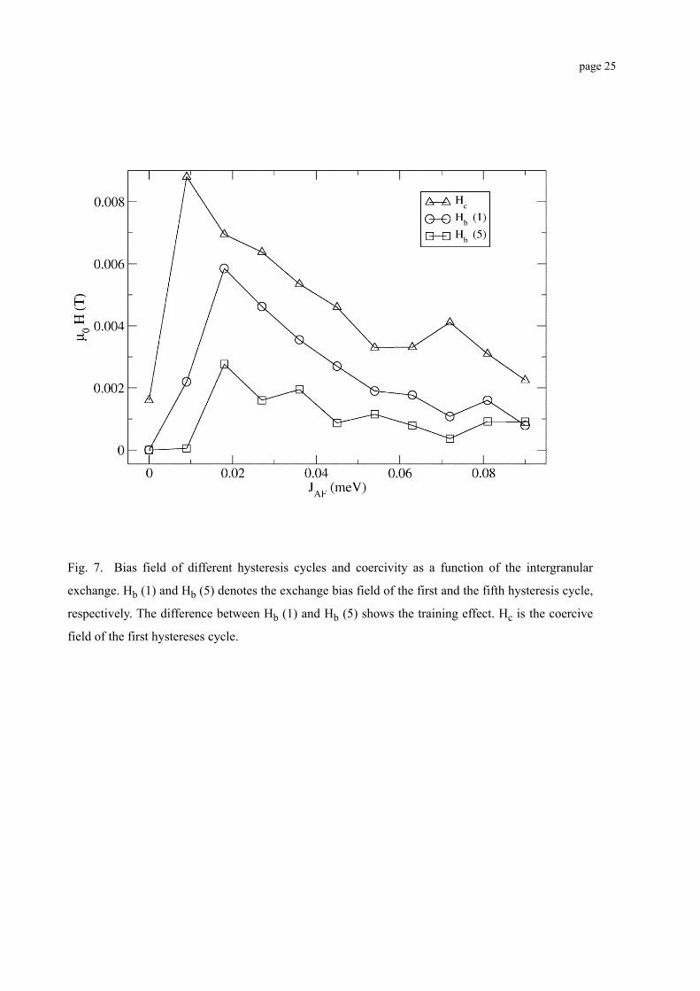
The complicated history dependence demonstrated during cycling is due to competition between

ferromagnetic and antiferromagnetic components of the grains originating in interlayer and inter-

grain exchange interactions. These dependencies are illustrated in Fig. 7 where the bias field and

coercivity are shown as a function of intergranular exchange. The coercivity is shown by triangles,

and is measured as the zero magnetization width of the first hysteresis loop. The maximum coer-

civity occurs for small nonzero values of intergranular exchange and represents the low energy

involved with irreversibly switching grains. The coercivity decreases almost linearly with increas-

ing intergranular exchange as the energy cost of reversing grains increases.

The bias field as a function of intergranular exchange for the first magnetization loop is indicated

by circles. The bias shift depends on intergranular exchange JAF in different manner than the coer-

civity because of how the bias depends upon reversible changes in the antiferromagnetic order.

Because of this, the first loop bias has a maximum for a JAF at about 0.02 meV, somewhat larger

than the value corresponding to the maximum in coercivity. The bias shift is reduced for larger JAF

as it becomes energetically less favorable to create misalignment between neighboring grains.

The bias field as a function of JAF is shown in Fig. 7 with squares for the fifth magnetization loop.

A weak maximum appears again for JAF at about 0.02 meV, but the overall magnitude of the bias is

page 11

much reduced from that of the first loop. As mentioned above, this training effect is a consequence

of how the system approaches a low energy steady state configuration.

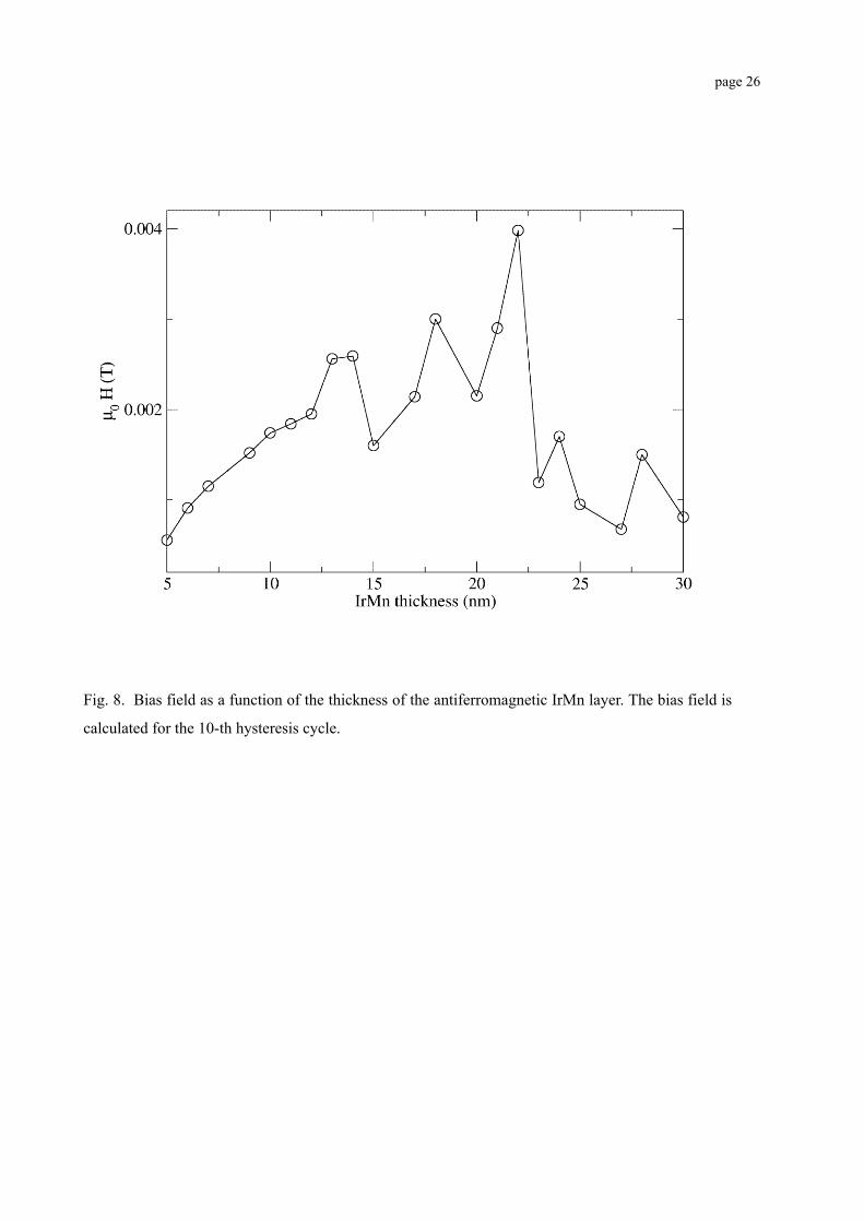
A quantity related to the intergrain exchange energy is the thickness of the antiferromagnetic film.

The contact area between grains controls the intergranular exchange energy. The intergranular

energy density therefore scales with film thickness. For this reason, the exchange terms in Eq. (1)

depend on the thickness of the antiferromagnet. The antiferromagnet thickness is therefore an

experimentally accessible parameter that affects directly the interaction between grains.

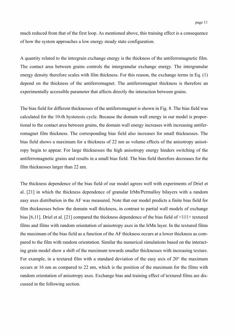
The bias field for different thicknesses of the antiferromagnet is shown in Fig. 8. The bias field was

calculated for the 10-th hysteresis cycle. Because the domain wall energy in our model is propor-

tional to the contact area between grains, the domain wall energy increases with increasing antifer-

romagnet film thickness. The corresponding bias field also increases for small thicknesses. The

bias field shows a maximum for a thickness of 22 nm as volume effects of the anisotropy anisot-

ropy begin to appear. For large thicknesses the high anisotropy energy hinders switching of the

antiferromagnetic grains and results in a small bias field. The bias field therefore decreases for the

film thicknesses larger than 22 nm.

The thickness dependence of the bias field of our model agrees well with experiments of Driel et

al. [21] in which the thickness dependence of granular IrMn/Permalloy bilayers with a random

easy axes distribution in the AF was measured. Note that our model predicts a finite bias field for

film thicknesses below the domain wall thickness, in contrast to partial wall models of exchange

bias [6,11]. Driel et al. [21] compared the thickness dependence of the bias field of <111> textured

films and films with random orientation of anisotropy axes in the IrMn layer. In the textured films

the maximum of the bias field as a function of the AF thickness occurs at a lower thickness as com-

pared to the film with random orientation. Similar the numerical simulations based on the interact-

ing grain model show a shift of the maximum towards smaller thicknesses with increasing texture.

For example, in a textured film with a standard deviation of the easy axis of 20° the maximum

occurs at 16 nm as compared to 22 nm, which is the position of the maximum for the films with

random orientation of anisotropy axes. Exchange bias and training effect of textured films are dis-

cussed in the following section.

page 12

IV. ANTIFERROMAGNETIC FILMS WITH TEXTURE

The above results assumed a flat distribution of anisotropy axes over all possible orientation

angles. This is not the best approximation of actual experimental samples where the structure of

granular materials may show on average a preferred orientation for crystalline axes. For example,

King et al. [22], conclude from x-ray diffraction patterns taken on NiFe/IrMn bilayers that the

granular IrMn layer is textured with the <111>-direction of the grains perpendicular to the inter-

face.

In terms of magnetic anisotropies, such texturing corresponds to an average angle between the easy

axis and the interface normal θ = 54.74o. In order to describe texture in our model, we have calcu-

lated bias shifts and coercivities with an angular distribution of anisotropy easy axes orientations.

A Gaussian distribution of angles θ measured between the film normal and the easy axis is

assumed:

. (3)

The width of the distribution is given by the parameter σ.

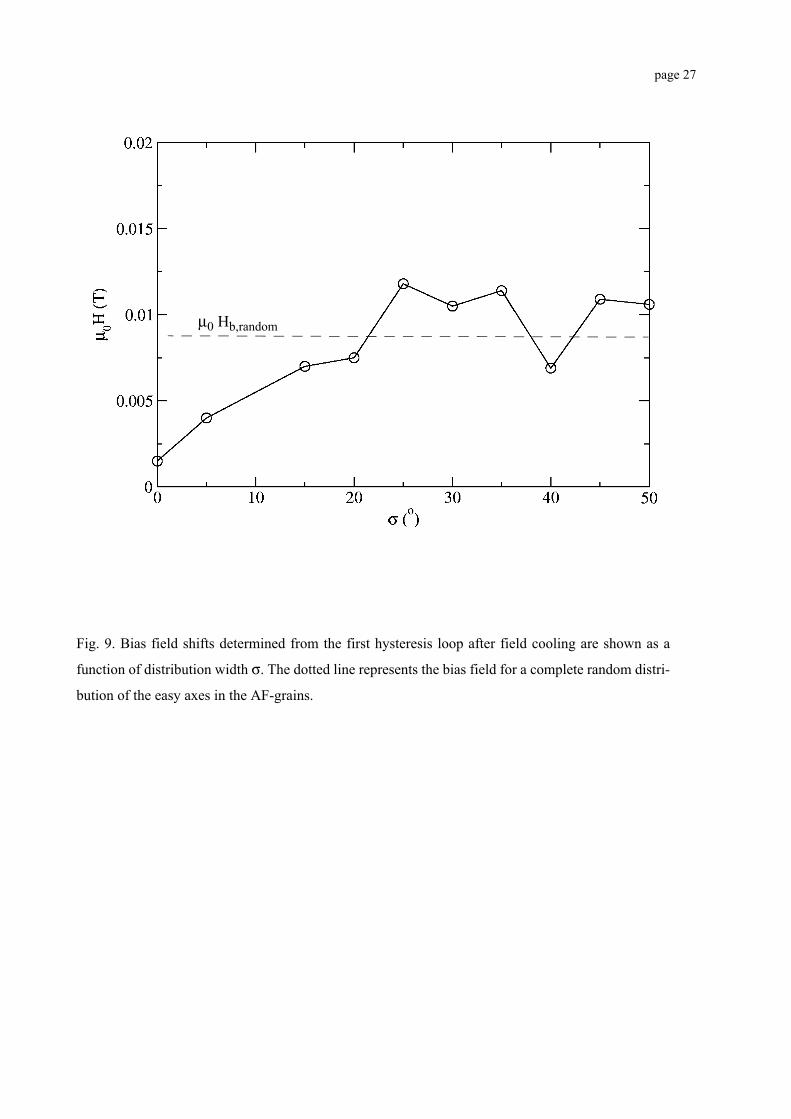
Bias field shifts determined from the first magnetization loop after field cooling are shown as a

function of distribution width σ. The following material parameters were used: JF= 0.23 meV,

JAF= 0.023 meV, JAF-F = -0.45 meV, tAF = 20 nm and tF = 10 nm. The average angle is assumed to

be θ = 54.74o. The bias shift exhibits a weak maximum for σ between 30o and 40o and remains

near a constant value of 0.01 T for σ greater than 45o.

The axes distribution has the largest effect on the bias field only when the spread in angles is small.

The angular range depends on the size and shape of the grains, and especially on the magnitude of

the intergranular exchange. A partial wall is stable only if the energy to irreversibly switch a grain

is larger than the energy of the wall. There is therefore a maximum angle through which partial

P θ( ) 12πσ

--------------e12--- θ θ–( )2

σ2-------------------–

θ( )sin=

page 13

twists between grains can form at each value of JAF. The range can be relatively narrow, as in the

example shown in Fig. 9, where this range is approximately ±20o.

In other words, only the fraction of grains with relatively well aligned axes contribute to bias shifts.

This means, for example, that bias fields for uniformly random axes distributions will in general be

less than bias fields for textured samples with all other factors being equal. This in fact what we

found upon comparing bias shifts for systems with texture, as shown in Fig. 9, to systems with axes

distributed randomly but uniformly on a sphere.

It is relevant to note that there is little dependence of the bias shift on the shape of the distribution

for such a narrow angular range. In consequence, the bias field shift calculated using a uniform dis-

tribution of axes restricted to a range of magnitude σ is little different from that calculated using a

gaussian distribution of width σ.

In contrast to the bias field, the coercive field is not as strongly affected by the width of the distri-

bution. Coercivity exists because of irreversible rotations of the ferromagnet, to which irreversible

processes in the antiferromagnet also contribute. It is interesting to examine the dependence of the

numbers of grains switched in the antiferromagnet to bias and coercive fields for different anisot-

ropy axis distribution widths. A summary is given in Table I where bias and coercive fields for dif-

ferent σ are listed together with the percentage of antiferromagnet grains switched during the

magnetization loop.

The number switched is determined at the zero field points of the first magnetization loop made

after field cooling. Switching for canted antiferromagnet sublattice magnetizations is defined in

terms of the l introduced in Fig. 1. Switching is said to occur when the component of l along the

anisotropy direction of a grain changes sign.

There is a clear correlation between the width of the distribution σ, percentage of switched grains

and the bias shift. Less clear is the relation between σ, the percentage of switched grains and the

coercive field. A key point in the bias mechanism proposed here is that switching of grains in the

antiferromagnet contributes to both bias field and coercivity observed through the ferromagnet.

However the bias shift depends exclusively on the formation of domain walls between grains.

page 14

These walls do not form unless some, but not all, antiferromagnets switch. Example percentages of

walls formed are listed in Table I for different axes distribution widths. The percentages are mea-

sured as the number of misaligned neighboring grains relative to the total number of possible mis-

alignments. Misalignment is defined for a pair if one grain has switched but other has not.

V. SUMMARY AND CONCLUSIONS

In this paper a type of partial wall model of exchange bias has been presented in which the partial

walls are formed along the interface in a granular antiferromagnetic film. The mechanism is simi-

lar to that proposed by Malozemoff except that our mechanism describes both coercivity and bias

through walls localized between grains, and applies directly to systems with interfaces compen-

sated at an atomic scale. We have shown that a relatively simple model can be used to quantify bias

and coercivity fields with predicted magnitudes on an order comparable to those observed experi-

mentally. The main conclusion is that the important mechanism governing bias in the random gran-

ular antiferromagnet is the intergrain exchange coupling. The proposed mechanism contributes to

exchange bias whenever the domain structure in the antiferromagnet changes during the reversal of

the ferromagnet. A key point is that irreversible switching in the antiferromagnet is therefore nec-

essary for bias field formation. Coercivity observed through the ferromagnet may be enhanced by

irreversible switching in the antiferromagnet, but ferromagnetic coercivity can also exist indepen-

dently.

The mechanism for bias proposed here applies only for grains which are smaller than an antiferro-

magnet wall width. One consequence is that our results are strictly valid only for intergrain

exchange coupling that is weak compared to the intragrain exchange so that a partial wall cannot

form within a grain. Furthermore, the weak intergrain exchange coupling is important for the irre-

versible switching of some grains which is a necessary component of our model. In the limit of

vanishing intergrain exchange, the finite element calculations show that it is not possible to reverse

grains in a thin antiferromagnetic film if the easy axis is not parallel to the interface.

page 15

The results of the granular partial wall model are in good agreement with calculations made using

a finite element solution which allows for nonuniform magnetization within grains. The only addi-

tional features revealed by finite element calculations are additional dependencies on grain height

and intergrain coupling in the limit of strong intergranular exchange. The grain height dependence

is in fact very important as the mechanism we propose only works for thin antiferromagnetic films.

Using finite element models for thick antiferromagnetic films, we find that the bias has a maxi-

mum at a small antiferromagnetic film thickness, and decreases to zero for very thick antiferro-

magnetic grains. The reason for this is that the anisotropy energy contained in the grains, which is

proportional to the grain volume, becomes larger than the intergranular exchange energy.

Work supported by the Austrian Science Fund, Y-132 PHY. RLS and JK also knowledge support

from the Australian Research Council.

page 16

REFERENCES

[1] W. H. Meiklejohn, C. P. Bean, Phys. Rev. 102, 1413 (1956).

[2] J. Nogués and K. Schuller, J. Magn. Magn. Mater. 192, 203 (1999).

[3] T. Ambrose, R. L. Sommer and C. L. Chien, Phys. Rev. B 56, 83 (1997).

[4] V. I. Nikitenko, V. S. Gornakov, L. M. Dedukh, Yu. P. Kabanov, and A. F. Khapikov, Phys. Rev. B 57, 8111 (1998).

[5] N. C. Koon, Phys. Rev. Lett. 78, 4865 (1997).

[6] T. C. Schulthess, W. H. Butler, Phys. Rev. Lett. 81, 4516 (1998).

[7] A. E. Berkowitz, J. H. Greiner, J. Appl. Phys. 36, 3330 (1965).

[8] L. Neel, Ann. Phys. 2, 61 (1967).

[9] H. Fujiwara, K. Zhang, T. Kai, T. Zhao, J. Magn. Mat. 235, 319 ( 2001).

[10]A. P. Malozemoff, J. Appl. Phys. 63, 3874 (1988).

[11]D. Mauri, H. C. Siegmann, P.S. Bagus und E. Kay, J. Appl. Phys. 62, 3047 (1987).

[12]A. I. Morosov, A. S. Sigov, J. Magn. Magn. Mater. 242-245, 1012 (2002).

[13]T. C. Schulthess and W. H. Butler, J. Appl. Phys. 85, 5510 (1999).

[14]U. Nowak, A. Misra, and K.D. Usadel, J. Appl. Phys. 89, 7269 (2001).

[15]D. Suess, T. Schrefl, W. Scholz, J. V. Kim, R. L. Stamps, J. Fidler, IEEE Trans. Magn., 38, 2002, in press.

[16]M. D. Stiles and R. D. McMichael, Phys. Rev. B 59, 3722 (1999).

[17]R. L. Stamps, J. Phys. D:Appl. Phys. 33, 247 (2000).

[18]J. C. Mallinson, IEEE Trans. Magn. 30, 62 (1987).

[19]A. C. Hindmarsh and L. R. Petzold, Computers in Physics 9, 148 (1995).

[20]D. Hinzke and U. Nowak, Phys. Rev. B 58, 265 (1998).

[21]J. van Driel, F. R. de Boer, K.-M. H. Lenssen and R. Coehoorn, J. Appl. Phys. 88, 975, 2000.

[22]J P King, J N Chapman, M F Gillies, J C S Kools, J Phys D: Appl Phys, 34, 528, (2001).

page 17

TABLE

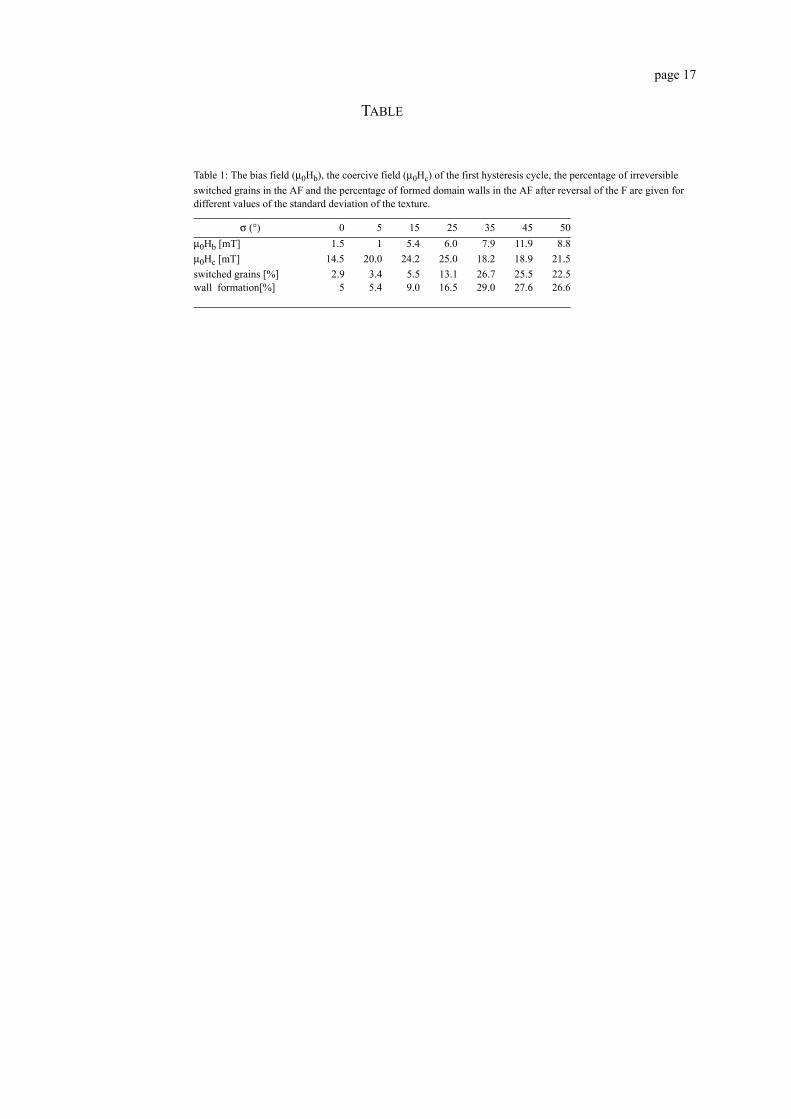
Table 1: The bias field (µ0Hb), the coercive field (µ0Hc) of the first hysteresis cycle, the percentage of irreversible switched grains in the AF and the percentage of formed domain walls in the AF after reversal of the F are given for different values of the standard deviation of the texture.

σ (°) 0 5 15 25 35 45 50µ0Hb [mT] 1.5 1 5.4 6.0 7.9 11.9 8.8µ0Hc [mT] 14.5 20.0 24.2 25.0 18.2 18.9 21.5switched grains [%] 2.9 3.4 5.5 13.1 26.7 25.5 22.5wall formation[%] 5 5.4 9.0 16.5 29.0 27.6 26.6

page 18

FIGURES

page 19

t = a + b

l = a - b a

b

(a) (b)

(c)

t1

l1

t2

l2

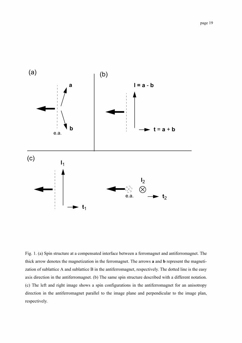
Fig. 1. (a) Spin structure at a compensated interface between a ferromagnet and antiferromagnet. The

thick arrow denotes the magnetization in the ferromagnet. The arrows a and b represent the magneti-

zation of sublattice A and sublattice B in the antiferromagnet, respectively. The dotted line is the easy

axis direction in the antiferromagnet. (b) The same spin structure described with a different notation.

(c) The left and right image shows a spin configurations in the antiferromagnet for an anisotropy

direction in the antiferromagnet parallel to the image plane and perpendicular to the image plan,

respectively.

e.a.

e.a.

page 20

F

fe

in

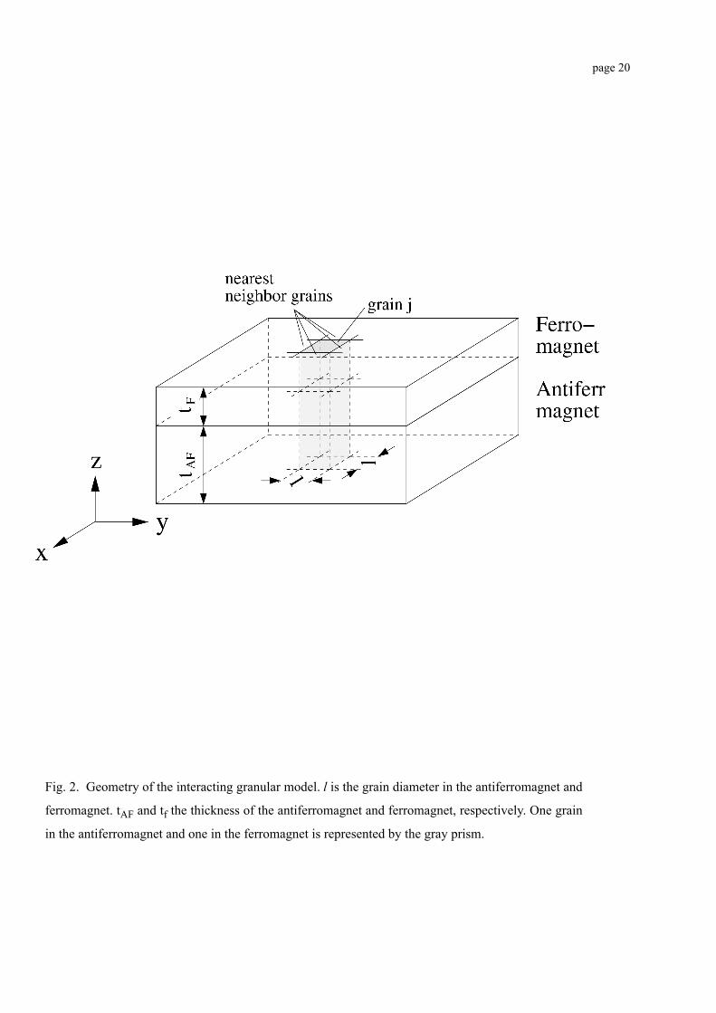
ig. 2. Geometry of the interacting granular model. l is the grain diameter in the antiferromagnet and

rromagnet. tAF and tf the thickness of the antiferromagnet and ferromagnet, respectively. One grain

the antiferromagnet and one in the ferromagnet is represented by the gray prism.

page 21

Fig. 3. Calculated hysteresis loops for a IrMn/Permalloy bilayer. The IrMn thickness and the grain

size is 20 nm and 10 nm, respectively. The thickness of the ferromagnet is 10 nm. The interface is

completely compensated. The bias field decreases with the number of hysteresis cycles.

page 22

Fig. 4. Domains in the antiferromagnet. The x-component of one antiferromagnet sublattice is indi-

cated by a gray scale. The properties of the antiferromagnet are the same as in Fig. 3. (A) state after

field cooling. µ0Hext = 0.1 T. (B) µ0Hext = -0.1 T. (C) Domain structure after the first hysteresis

cycle. µ0Hext = 0.1 T. (D) µ0Hext = -0.1 T.

120 nm

A B

C D

x

y

Jx (Js)

-1 0 1

page 23

Fig. 5. Spin configuration of an granular AF/F bilayer after field cooling and after the reversal of the

ferromagnet, respectively. The magnetization of one sublattice is shown in the antiferromagnet. The

easy axis of G1 is parallel to the AF/F interface. The angle between the easy axis of G2 and the inter-

face is 10°. After field cooling the magnetization of the two grains points almost parallel. After

switching of the ferromagnet only G2 reverses.

field cooled state reversed state

G2 G2G1 G1

page 24

Fig. 6. Exchange energy in the AF as a function of the external field strength for the first and second

hysteresis cycle. The states (A) - (D) are the same as in Fig. 4.

A

C

BD

page 25

Fig. 7. Bias field of different hysteresis cycles and coercivity as a function of the intergranular

exchange. Hb (1) and Hb (5) denotes the exchange bias field of the first and the fifth hysteresis cycle,

respectively. The difference between Hb (1) and Hb (5) shows the training effect. Hc is the coercive

field of the first hystereses cycle.

page 26

Fig. 8. Bias field as a function of the thickness of the antiferromagnetic IrMn layer. The bias field is

calculated for the 10-th hysteresis cycle.

page 27

Fig. 9. Bias field shifts determined from the first hysteresis loop after field cooling are shown as a

function of distribution width σ. The dotted line represents the bias field for a complete random distri-

bution of the easy axes in the AF-grains.

µ0 Hb,random