Embed Size (px)
Citation preview
Highlights
We propose a growth cycle accounting procedure to estimate the long-run elasticity between growth and finance.
This procedure links long-run growth to the duration and growth rate of expansions and recessions.
The elasticity between financial and economic growth rates is positive for a complete business cycle, even if high financial growth makes recessions more severe.
This elasticity may turn negative if one considers the persistent effects of financial growth on the expansion of the subsequent cycle.
Excess Finance and Growth: Don't Lose Sight of Expansions !
No 2015-31 – December Working Paper
Thomas Grjebine & Fabien Tripier
CEPII Working Paper Excess Finance and Growth: Don’t Lose Sight of Expansions !
Abstract Accompanying the great recession, a recent empirical literature casts doubt on the existence of a positive relationship between economic and financial growth pointing out the economic costs of excessive financial growth. We show however that if one considers the complete growth cycle, that is by including expansions into a growth cycle accounting procedure, the elasticity between financial and economic growth rates is positive for most financial series, even if high financial growth makes recessions more severe. This elasticity should be however adjusted downward, and may even turn negative, if one considers the persistent effects of financial growth on the expansion of the subsequent cycle. This effect can explain the pattern of economic growth observed during and after financial bubbles.
KeywordsGrowth, Business Cycles, Finance, Financial Cycles, Bubbles.
JELE32, E44.
CEPII (Centre d’Etudes Prospectives et d’Informations Internationales) is a French institute dedicated to producing independent, policy-oriented economic research helpful to understand the international economic environment and challenges in the areas of trade policy, competitiveness, macroeconomics, international finance and growth.
CEPII Working PaperContributing to research in international economics
© CEPII, PARIS, 2015
All rights reserved. Opinions expressed in this publication are those of the author(s) alone.
Editorial Director: Sébastien Jean
Production: Laure Boivin
No ISSN: 1293-2574
CEPII113, rue de Grenelle75007 Paris+33 1 53 68 55 00
www.cepii.frPress contact: [email protected]
Working Paper
CEPII Working Paper Excess Finance and Growth: Don’t Lose Sight of Expansions !
Excess Finance and Growth: Don’t Lose Sight of Expansions !
Thomas Grjebine,∗ and Fabien Tripier†
"How long has it been since the American economy enjoyed reasonable growth, from a reasonable
unemployment rate, in a financially sustainable way? The answer is that is has been really quite a
long time, certainly more than half a generation". Summers (2015)
"We may be an economy that needs bubbles just to achieve something near full employment".
Krugman (2013)
1. Introduction
The "Secular Stagnation" debate launched by Summers (2013) and Krugman (2013) has recently revived
the attention on the difficulties to conciliate economic growth with financial stability. They raise in
particular the question of what would have been growth during the last thirty years in developed economies
without financial and housing bubbles. This debate highlights the complexity of the interactions between
economic growth and finance, which has been alternatively pointed out as a key driver of economic growth
and a major source of amplification of economic crisis. This paper proposes a new empirical methodology,
labeled growth cycle accounting, which provides an unified framework to estimate and compare these
different effects. Even if high financial growth makes recessions more severe, the elasticity between
finance and growth for a complete business cycle is positive because of the key role played by expansions.
This positive elasticity should however be adjusted downward by the excessive development of finance
inherited from previous expansions. Hence, don’t lose sight of expansions!
∗CEPII ([email protected])†Univ. Lille 1 - CLERSE & CEPII ([email protected])
3
CEPII Working Paper Excess Finance and Growth: Don’t Lose Sight of Expansions !
If the two faces of finance, key driver of economic growth and major source of instability are well
known, quite surprisingly, they are based on stylized facts established in distinct frameworks, with separate
data and empirical tools. A large empirical literature on long-run growth has been developed in the tradition
of King and Levine (1993) after the precursory contributions of Goldsmith (1969) and McKinnon (1973).
The starting point of this literature is to regress long-run growth for a panel of country on a set of variables
among which one of them measures the initial state of development of the financial sector and the other
are control variables. This literature concluded on the existence of a positive and significant relationship
between average growth and various measures of financial development, see Levine (1997), even if recent
studies have challenged the robustness of this conclusion as Cecchetti and Kharroubi (2012), Rousseau
and Wachtel (2011, 2015) or Arcand et al. (2015). To take into account the time-varying behavior of the
financial sector, these studies estimate dynamic panels using window of several years (generally five years)
to eliminate business cycle fluctuations.
Another recent literature focuses precisely on business cycle fluctuations to identify the links between
financial development and economic crisis. Actually, they do not consider all business cycle fluctuations,
but they focus instead on the recessions’ characteristics, that is the probability of occurrence, the severity,
and the duration. Drehmann et al. (2012) show that financial cycle peaks are very closely associated with
financial crises and business cycle recessions are much deeper when they coincide with the contraction
phase of the financial cycle; Claessens et al. (2012) that the duration and amplitude of recessions are
higher when they occur with financial disruptions; Jordà et al. (2013) that the severity of recessions is
amplified by the intensity of financial development; and Schularick and Taylor (2012) that the credit ratio
is a good predictor of financial crisis1. In this literature, less attention is given to economic expansions,
which however determine the long-run growth when cumulated over the cycles of an economy.
To sum up, the literature on growth does not consider the specificity of business cycle phases1See also Borio et al. (2013) who develop measures of potential output and output gaps in which financial factors play a
central role.
4
CEPII Working Paper Excess Finance and Growth: Don’t Lose Sight of Expansions !
while the literature on recessions does not take into account the economic growth process associated
with the expansion phases. In this article, we fill the gap between these two strands of the literature
by providing a unified empirical framework, which we call a growth cycle accounting. This framework
allows to decompose the long-run elasticity between finance and growth as the sum of business cycle
elasticities. If this methodology is not suitable to identify causal relationships, as actually most previous
quoted references, it aims at identifying the regular pattern of interactions between economic and financial
growth both in the short- and the long-run. Our paper complements recent attempts in the literature to
balance the various interactions between finance and growth. Ranciere et al. (2006) develop a setup to
decompose the effects of financial liberalization on economic growth and on the incidence of crises. To
do so, they introduce crisis events into standard growth regressions augmented with financial variables.
This setup allows to compare the direct effect of financial liberalization on growth, which is close to the
one identified by Levine (1997) and others, and the indirect effect, which is negative and results from
the occurrence of financial crises2. In a similar manner, Bonfiglioli (2008) studies the effects of financial
globalization on investment and productivity growth by controlling for indirect effects on banking and
currency crisis.
The key point of our approach is that we do not split series into trend and cyclical components
by removing a trend from original series to get the classical cycle. Instead, we study the growth cycle
which is defined by the analysis of turning points (known as peaks and troughs) between expansion and
recession phases.3 The interest of this set-up is to link the long-run economic growth to the properties
of business cycles. Indeed, the long-run growth of an economy is equal to the average growth observed
2Rancière and Tornell (2015) develop a two-sector model consistent with these empirical facts in which financial liberalization
may increase growth, but leads to more crises and costly bailouts.3Gadea Rivas and Perez-Quiros (2015) study the relations between credit and growth both during expansion and recession
phases, as we do, but with a different objective. The authors’ objective is to assess the ability of credit-based indicators to
forecast efficiently the recessions. They show the poor performances of credit-based indicators in out of sample prediction
of crisis because of the procyclical behavior of credit, which increases during expansion.
5

CEPII Working Paper Excess Finance and Growth: Don’t Lose Sight of Expansions !
for all growth cycles of this economy. Then, it is possible to get insights for long-run economic growth by
analysing the properties of growth cycles – it is not the case for classical cycles which are by construction
independent on the trend of long-run growth. Therefore, instead of looking directly at the relationship
between long-run growth and finance, we investigate the relationship between growth cycles and finance
and then draw some conclusions for long-run growth. To do that, we show that the elasticity between
long-run growth and finance can be expressed as the sum of elasticities associated with the growth cycle
properties – hence, the label growth cycle accounting proposed for this methodology. The finance-growth
elasticity in the long-run can be viewed as the cumulative of finance-growth interactions within each
cycle through two channels: (i) the growth channel, associated with the difference in the growth rates
between the expansion and recession phases, and (ii) the duration channel, associated with the difference
in the durations of the expansion and recession phases. The procedure allows to assess the statistical
significativity of each channel and to quantify their relative importances to provide a global picture of
the finance-growth interactions. The growth cycle accounting procedure is also of interest to study the
interactions between financial and the volatility of economic growth.
The application of the growth cycle accounting methodology requires an empirical measure for
finance. The recent empirical literature uses measures of financial activities around the peaks of economic
activity to assess their interactions with economic growth during the recessions, see Drehmann et al.
(2012), Claessens et al. (2012), Schularick and Taylor (2012), and Jordà et al. (2013). Because we want
to balance these interactions with what happens during expansions, we follow these authors and consider
measures of financial activities at the peaks of business cycles. More precisely, we consider the growth rate
of financial series during the expansion phase for each growth cycle taken in deviation with the mean of
growth observed for all business cycles, as in Jordà et al. (2013), and label this measure "excess finance".
To take into account the persistent effects of financial growth during one growth cycle on the subsequent
cycles, we also include in our study the initial value of the financial series at the beginning of each growth
6
CEPII Working Paper Excess Finance and Growth: Don’t Lose Sight of Expansions !
cycle. The growth cycle accounting procedure is applied to a panel of 25 countries over the period 1970-
2015. Business cycles are defined by the identification of turning points in the real GDP per capita for
each country. We take house prices as the benchmark for the financial series. Results are then compared
with other series related to the housing sector, namely the price to rent and price to income series and
with series related to the credit market, namely real credit and credit to GDP ratio for the private sector
as a whole or only for households.
Following Arcand et al. (2015), we control for endogeneity of our regression models using the esti-
mators developed by Rigobon (2003) and Lewbel (2012) that allow to identify causal relationships through
heteroskedasticity. In the presence of heteroskedasticity in the regression’s residual, this methodology al-
lows identifying causal relationships even in the absence of external instruments. We show that our results
are robust to controlling for endogeneity with this technique.
Our first result is that the long-run elasticity between economic and excess finance is positive. For
example, for house prices, the elasticity is equal to 14.7%4. This elasticity is the sum of the elasticities
linked to the growth channel (12.4%) and the duration channel (1.9%). Looking at the growth channel,
the elasticity is positive during the expansion (20.1%) and turns negative during the recession phase (-
7.7%).5 This result is close to that of Ranciere et al. (2006) and Bonfiglioli (2008) who conclude that
the direct positive effect of financial development on growth outweighs the indirect and negative effect
associated with crisis occurrence. However, this result does not take into account the persistent effects
of excess finance on subsequent cycles trough the initial value of financial series. Actually, we show that
the long-run elasticity between economic growth and the initial value of financial series is negative for all
series. This result is of importance because is suggests that positive elasticity within business cycles should
be adjusted downward by persistence effects between growth cycles. This situation can be interpreted as
4 This number should be interpreted as follows: a 1% excess finance is associated in the data with a variation of 0.14
points of percentage of annual growth in the long run.5The sum of these two elasticities is the value of the growth channel (12.4%).
7
CEPII Working Paper Excess Finance and Growth: Don’t Lose Sight of Expansions !
a hysteresis phenomenon – see Blanchard et al. (2015) and Galí (2015) for recent contributions on the
importance of the concept of hysteresis to understand the full consequences of recessions. We use our
regression results to simulate the pattern of economic growth associated with financial bubbles defined as
the alternation of highly positive and negative financial growth rates with persistent effects. Our results
show that financial bubbles are characterized by a long phase of expansion together with high economic
growth. They are ended by a more severe recession, as already well documented in the literature, but are
also followed by a depressed growth cycle characterized by low economic growth and a short expansion
phase.
The rest of the paper proceeds as follows. In Section 2, we describe the growth cycle accounting
procedure. We show in particular that the finance-growth elasticity in the long-run can be viewed as the
cumulative of finance-growth interactions within each cycle through two channels, the growth channel and
the duration channel. We show implications for volatility and we present the case of financial bubbles.
In Section 3, we present our empirical methodology. In Section 4, we present the results, both for the
regressions and the growth cycle accounting procedure. We also propose simulations of GDP patterns
depending on variations in excess finance. Finally, as robustness, we present the results for seven other
measures of excess finance.
2. The Growth Cycle Accounting Procedure
This section describes the growth cycle accounting procedure.
2.1. Growth Cycle
We consider a panel of n countries indexed by i = 1, ..., n and t = 1, ..., Ti where t is a quarter and Ti
the number of observations of the series for the country i. In the time domain, the real GDP per capita
is denoted Yi,t, which quarterly annual growth rate is denoted gi,t ≡ log (Yi,t/Yi,t−4).
To implement the growth cycle accounting procedure, the series should be defined in the dimension
8

CEPII Working Paper Excess Finance and Growth: Don’t Lose Sight of Expansions !
of economic cycles and not only in the time domain. For each country i, we observe c = 1, ..., Ci cycles.
For each cycle c, s = 1, ..., τc stands for the quarter of the cycle and τc for the duration of the cycle. The
cycle c can itself be decomposed into two business cycle phases: the expansion and the recession. In the
remainder, we use the following notation: xph refers to the value of the series x for the business cycle
phase ph, which can take two values ph = {ex, re} where ex stands for expansion and re for recession.
The duration of the growth cycle satisfies τc = τ exc + τ rec where τ exc is the duration of the expansion phase
and τ rec the duration of the recession phase. The peak of a typical business cycle is reached as of time
τ exc , which is the end of the expansion phase and the beginning of the recession phase, one quarter after.
The trough of the cycle corresponds to the period (τ exc + τ rec ) , which is the end of the recession and the
start of the next cycle, one quarter after. The phase ph represents the share πph = τ phc /τc of the duration
of the cycle c.
πph ≡ τ phcτ exc + τ rec
, for ph = {ex, re} (1)
In the cycle dimension, Yi,c,s denotes the real GDP per capita observed during the quarter s of the cycle
c in country i, which quarterly annual growth rate is denoted gi,c,s ≡ log (Yi,c,s/Yi,c,s−4).
The average growth rate of the real GDP for the panel of countries is denoted g and defined as
g ≡ 1n
n∑i=1
gi (2)
where gi denotes the average growth for the economy i. In the time domain, the average growth of a
country is calculated as gi ≡ (1/Ti)∑Tit=1 gi,c without taking into account the business cycle. The interest
of the cycle dimension, is to take into account potential differences between expansion and recession
business cycle phases. To do so, the average growth rate of the country i, namely gi, is calculated as the
average of growth rates for each cycle c, which is denoted gi,c, using the formula
gi ≡1Ci
Ci∑c=1
gi,c (3)
where gi,c can be expressed as the average of the growth rates during the expansion and recession phases,
respectively denoted gexi,c and grei,c, weighted by the share of each business cycle phase in the full duration
9
CEPII Working Paper Excess Finance and Growth: Don’t Lose Sight of Expansions !
of the cycle, namely πex and πre respectively, that is
gi,c ≡ πexi,cgexi,c + πrei,cg
rei,c (4)
where the averages of growth rates for each business cycle phase are defined as follows.
gexi,c ≡1τ exi,c
τexi,c∑s=1
gexi,c,s, and grei,c ≡1τ rei,c
τi,c∑s=τex
i,c+1grei,c,s (5)
These definitions of growth are used hereafter to compute the elasticity of growth with respect to financial
series.
2.2. Financial Properties of Growth Cycles
As for the real GDP per capita, we define financial series in the cycle dimension: Fi,c,s denotes the value
of the financial series F measured for the quarter s of the cycle c in country i. We do not consider herein
the specific cycles of the financial series. Then, the timing of expansion and recession of business cycle
phases is the same as for the real GDP per capita. Actually, we are interested by the properties of growth
cycles in terms of financial activities. For each financial series considered, the state of financial activies is
defined by its excess growth during the expansion phase
φexi,c ≡log
(Fi,c,τex
i,c/Fi,c,0
)τ exi,c
− φ̃ex (6)
which is the quarterly average growth rate of F during the expansion phase in deviation with φ̃ex, the
average of growth rates for all the cycles of all the countries of the panel, namely
φ̃ex ≡ 1n
n∑i=1
1Ci
Ci∑c=1
log(Fi,c,τex
i,c/Fi,c,0
)τ exi,c
(7)
We then use this definition of excess finance to measure the links between financial and growth cycle.
10
CEPII Working Paper Excess Finance and Growth: Don’t Lose Sight of Expansions !
2.3. The Finance-Growth Elasticities
The semi-elasticity of long-run growth rate g with respect to the measure of excess finance φex is given
by the following first order partial derivative
εgφex ≡∂g
∂φex(8)
Since both g and φex are the log of "gross" growth rates of real GDP per capita and the financial series,
εgφex is the semi-elasticity between these two rates and the elasticity between these two "gross" rates. For
simplicity, we use the term elasticity for εgφex in the remainder while keeping in mind that it concerns the
"gross" rates of series. Using (1), (2) and (3), the long-run growth rate is
g = 1n
n∑i=1
1Ci
Ci∑c=1
(πexi,cg
exi,c + πrei,cg
rei,c
)(9)
where the number of countries n and of cycles by countries Ci are independant on the value of financial
series. Then, using (9), the elasticity εgφex defined by (8) is equal to
εgφex = 1n
n∑i=1
1Ci
Ci∑c=1
∂gexi,c∂φex
τ exi,cτ exi,c + τ rei,c
+∂grei,c∂φex
τ exi,cτ exi,c + τ rei,c
+(∂τ exi,c∂φex
τ rei,c −∂τ rei,c∂φex
τ exi,c
)gexi,c − grei,c(τ exi,c + τ rei,c
)2
(10)
where ∂gphi,c/∂φex are the elasticities of growth with respect to excess finance for each business cycle phase
ph = {ex, re} of the growth cycle. Using (5) these partial derivatives are
∂gexi,c∂φex
= 1τ exi,c
τexi,c∑s=1
∂gexi,c,s∂φex
, and∂grei,c∂φex
= 1τ rei,c
τi,c∑s=τex
i,c+1
∂grei,c,s∂φex
(11)
since the durations are assumed to be constant when the partial derivatives of gphi,c with respect to φex
are computed for ph = {ex, re}. We use two kinds of regression to quantify the terms present in the
equation (10) of the long-run elasticity. First regressions consider the growth rate during business cycle
phases as a dependent variable and the second regressions consider the duration of business cycle phases
as a dependent variable.
Growth regressions are estimated with the standard OLS estimator using the following specification
gphi,c,s = cphg + fphg,i + αphg φex + γphg X
gi,c,s + εi,c,∫ (12)
11
CEPII Working Paper Excess Finance and Growth: Don’t Lose Sight of Expansions !
for each phase ph = {ex, re} . In this regression, cphg is the constant term, fphg,i a country-fixed effect, Xgi,c,s
is a set of controls for both business cycles and growth, and αphg the coefficient of interest that measures
the elasticity between growth and excess finance during the business cycle phase ph = {ex, re}. Using,
(12) the elasticity of growth with respect to excess finance during the business cycle phase ph writes
∂gphi,c∂φex
= 1τ phi,c
τphi,c∑s=1
αphg = αphg (13)
for ph = {ex, re} .
Duration regressions are estimated with the Accelerated Failure-Time (AFT) specification of the
Weibull model developed for duration data with covariates. Assuming that the duration τ ph of the
business cycle phase ph = {ex, re} has a Weibull distribution, the logarithm of duration τ ph can be
estimated using the following specification
log(τ phi,c
)= cphτ + fphτ,i + αphτ φ
ex + γphg Xτi,c + zphi,c (14)
where zphi,c has an extreme-value distribution scaled by the inverse of the shape parameter of the Weibull
distribution, denoted pph. In this regression, cphτ is the constant term, fphτ,i a country-fixed effect, Xτi,c,s is
a set of controls for both business cycles and growth, and αphτ the coefficient of interest. Using (14), the
(semi-)elasticity of the duration of the business cycle phase ph with respect to excess finance is
∂τ phi,c∂φex
= αphτ τphi,c (15)
for ph = {ex, re}.
The elasticity defined by (10) becomes
εgφex = 1n
n∑i=1
1Ci
Ci∑c=1
αexg(
τ exi,cτ exi,c + τ rei,c
)+ αreg
(τ exi,c
τ exi,c + τ rei,c
)+ (αexτ − αreτ )
τ exi,c τrei,c(
τ exi,c + τ rei,c)2
(gexi,c − grei,c
)(16)
given the outcomes of the regressions (13) and (15), details are provided in the appendix A. Then, since
12
CEPII Working Paper Excess Finance and Growth: Don’t Lose Sight of Expansions !
the regression coefficients do not depend on the country i or the cycle c, the equation (16) becomes
εgφex = αexg1n
n∑i=1
1Ci
Ci∑c=1
πexi,c + αreg1n
n∑i=1
1Ci
Ci∑c=1
πrei,c + αexτ1n
n∑i=1
1Ci
Ci∑c=1
σexi,c + αreτ1n
n∑i=1
1Ci
Ci∑c=1
σexi,c (17)
The new variable σi,c is defined as follows
σi,c ≡ πexi,cπrei,c
(gexi,c − grei,c
)(18)
This variable provides a measure the gap in growth rates between the two business cycle phases, namely
(gexi,c − grei,c), weighted by the relative duration of business cycle phases, πexi,c and πrei,c. Considering the
historical mean of πexi,c, πrei,c, and σi,c for all cycles of the panel, the elasticity given by (17) becomes
εgφex = αexg × π̃ex + αreg × π̃re︸ ︷︷ ︸Growth Channel
+ (αexτ − αreτ )× σ̃︸ ︷︷ ︸Duration Channel
(19)
where x̃ denotes the historical mean of the series xi,c for x = {πex, πre, σ}.
The long-run elasticity of growth with respect to excess finance is the sum of three elements which
are directly associated with business cycle properties. The sum of the first two elements constitutes the
growth channel since it depends on the elasticities of growth during business cycle phases with respect to
excess finance, namely αexg and αreg , which are weighted by the relative shares of expansions and recessions
in the business cycle duration, namely π̃ex and π̃re. The third element constitutes the duration channel
since it depends on the elasticities of business cycle phase durations with respect to excess finance, namely
αexτ and αreτ , and the weighted gap in the growth rates, which is measured by σ̃. The duration channel
does not exist if at least one of these three conditions is satisfied
1. the duration of business cycle phases are not correlated with excess finance: αexτ = αreτ = 0;
2. the duration of business cycle phases are correlated with excess finance, but the elasticity is the same
for the two business cycle phases: (αexτ − αreτ ) = 0;
3. the duration of business cycle phases are correlated with excess finance, with different elasticities for
the two business cycle phases, but the weighted gap in growth rates between the two business cycle
phases is nil: σ̃ = 0.
13
CEPII Working Paper Excess Finance and Growth: Don’t Lose Sight of Expansions !
2.4. Implications for Volatility
The growth cycle accounting approach can also be used to study the implications of the properties of
business cycles on the volatility of the economy. We measure the volatility by the variance of the quarterly
annual growth of real GDP per capita, which is denoted var (g) for all the panel and defined as follows
var (g) ≡ 1n
n∑i=1
var (gi) (20)
where var (gi) is the variance of growth gi for each country i of the panel. Using the definition (3) of
growth in country i, the variance var (gi) is equal to
var (gi) ≡ var 1Ci
Ci∑c=1
gi,c
= 1Ci
Ci∑c=1
var (gi,c) +∑c 6=c′
cov (gi,c, gi,c′) (21)
that is the average value of variances observed for all cycles c of country i, namely var (gi,c), plus the
covariance of growth rates between cycles, namely cov (gi,c, gi,c′) for c 6= c′. As done in the previous
section for the average of growth, see (4), the variance of growth can be decomposed into contributions
of each business cycle phase as follows
var (gi,c) = πexi,cvar(gexi,c)
+ πrei,cvar(grei,c)
+ πexi,cπrei,c
(gexi,c − grei,c
)2(22)
Details are provided in the appendix B. The variance of growth during the cycle c in country i is the
sum of (i) the variances of growth during each business cycle phase, namely var(gphi,c)for ph = {ex, re},
weighted by the relative duration of business cycle phases, namely πphi,c for ph = {ex, re}, and of (ii) the
squared-gap of growth rates between expansion and recession phases, namely(gexi,c − grei,c
)2, also weighted
by the relative duration of business cycle phases, namely πexi,cπrei,c.
As for the average growth, regressions are estimated for the standard deviation of growth with an
OLS estimator using the following specification
sd(gphi,c)
= cphsd + fphsd,i + αphsdφex + γsdXτ
i,c + ε̃i,c (23)
14

CEPII Working Paper Excess Finance and Growth: Don’t Lose Sight of Expansions !
for each phase ph = {ex, re} . Notice that, following the tradition in the literature regressions are estimated
for the standard deviation of growth and not for the variance. In this regression, cphsd is the constant term,
fphsd,i a country-fixed effect, Xτi,c is a set of controls for both business cycles and growth, and αphsd the
coefficient of interest. The semi-elasticity of the standard deviation of growth during the business cycle
phase ph with respect to excess finance is deduced from regression (23) as
∂sd(gphi,c)
∂φex= αphsd (24)
Then, using (20), (21), (22), and (24), the semi-elasticity of the variance of growth with respect to excess
finance can be decomposed as follows
∂var (g)∂φex
= αexsd ×2n
n∑i=1
1Ci
Ci∑c=1
πexi,csd(gexi,c)
+ αresd ×2n
n∑i=1
1Ci
Ci∑c=1
πrei,csd(grei,c)
︸ ︷︷ ︸Volatility Channel
(25)
+(αexg − αreg
)×
n∑i=1
1Ci
Ci∑c=1
πexi,cπrei,c2
(gexi,c − grei,c
)︸ ︷︷ ︸
Growth Channel
+ (αexτ − αreτ )×n∑i=1
1Ci
Ci∑c=1
πexi,cπrei,c
[var
(gexi,c)− var
(grei,c)
+(gexi,c − grei,c
)2 (1− 2πexi,c
)]︸ ︷︷ ︸
Duration Channel
Details are provided in the appendix C. The volatility channel is associated with the variances of growth for
each phase of the business cycles. It is the weighted average of semi-elasticities of the standard deviation
of growth during each business cycle phase, namely αphsd for ph = {ex, re}, weighted by the relative
duration of business cycle phases, namely πphi,c for ph = {ex, re}. Even if these semi-elasticities are nil,
that is αexsd = αresd = 0, the variance of growth may be linked to excess finance through the two other
channels associated with the properties of business cycles: the growth channel and the duration channel.
The growth channel is associated with the volatility of the economy induced by the switch between two
business cycle phases characterized by different average growth rates. Indeed, this channel does not exist
if the growth rates are equal in the two business cycle phases, gexi,c = grei,c, or have the same elasticity
with respect to excess finance, αexg = αreg . The duration channel is associated with the volatility of the
15

CEPII Working Paper Excess Finance and Growth: Don’t Lose Sight of Expansions !
economy induced by the frequency of switch between the two business cycle phases. This channel does
not exist if the variance and the mean of growth rates are identical in the two business cycle phases, that
is both var(gexi,c)
= var(grei,c)and gexi,c = grei,c, or the elasticities of the business cycle phases with respect
to excess finance are equal, αexT = αreT .
To quantify the relative importance of these three channels for all the panel of countries, we use the
results of the regressions (12), (14), and (23) to get numerical values of the coefficients αphg , αphT , and
αphvar, respectively, for ph = {ex, re}. Historical data are used to compute the average values of the terms
that multiplied these regression coefficients in (26).
2.5. Persistent Effects of Excess Finance and The Case of Financial Bubbles
In the previous sections, the interactions between economic growth and financial growth were considered
within the same business cycle. However, current economic growth may also be related with past financial
growth through persistent effects. We now take into account this phenomenon, which may be important
to understand the consequences of financial bubbles.
Financial bubble is a very large concept to describe situations in which market prices diverge lastingly
from their fundamental or equilibrium values in such a way that market corrections should occur to restore
market equilibrium. In our data, financial growth is defined for financial series that try to capture such
divergence, as the price-to-rent ratio and credit-to-ouput. However, it is hard to distinguish in the data the
fluctuations of theses series that result from structural shifts of the economy from those that result from
purely bubble/speculative behaviors. Nevertheless, our methodology can be informative to characterize
the pattern of economic growth associated with a financial bubble. Once again, we do not measure here
the causal impact of a financial bubble on economic growth, but we identify the joint behavior of economic
16
CEPII Working Paper Excess Finance and Growth: Don’t Lose Sight of Expansions !
and financial growth during business cycles. A financial bubble during the cycle c̃ is defined as follows
φexc =
ε
−ε
0
, if c = c̃
, if c = c̃+ 1
otherwise
(26)
where ε is the size of the bubble. The symmetry of financial growth during cycles c̃ and (c̃+ 1) ensures
the full adjustment of the bubble for future cycles c > (c̃+ 1). In addition to the negative financial growth
during the cycle (c̃+ 1), the value of the financial series at the begining of this cycle is also impacted by
the bubble since
φ0c̃+1 = φ0
c̃ + φexc̃ (27)
where φ0c̃is the inital value of the financial series, that is for the quarter 0 of the cycle c̃. If economic
growth during the cycle c̃ + 1 is correlated with φ0c̃, it means that financial growth during the previous
cycle, namely φexc̃, has persistent effects for subsequent cycles. This situation can be interpreted as a
hysteresis phenomenon.
Hysteresis is a popular concept to depict situations in which the consequences of an action persist
even when this action is finished. In previous sections, the action considered was an excess in the growth
rate of financial series. The various measures of elasticity provided tried to capture the links between
this excess development of finance and the business cycle during which this excess occurred. However,
this excess can also have links with future cycles due to the hysteresis phenomenon. For example, an
excessive growth of house prices during a cycle can lead to a high house price level at the beginning of
the new cycle. In this case, even if housing prices are constant during this new cycle, the consequences
of the previous cycle are still present through the initial value of housing prices. To take into account this
possibility, we systemically consider in our regressions (12), (14), and (23) the initial value of the financial
series φ0i,c ≡ Fi,c,0 among the controls Xg
i,c,s and Xτi,c.
The elasticity of growth with respect to a financial bubble B during cycle c is then defined as the
17
CEPII Working Paper Excess Finance and Growth: Don’t Lose Sight of Expansions !
sum of the elasticities of economic growth with respect to a positive and a negative financial growth rates,
augmented with the elasticity with respect the inital condition of the financial series.
εgB ≡ ε∂g
∂φex+ ε
∂g
∂φ0︸ ︷︷ ︸Persistent Effect
−ε ∂g
∂φex(28)
Our previous regressions can be used to compute each of these terms. For long-run economic growth,
the first and third terms cancel naturally each other because financial growth is symmetric and only the
persistent effect (namely the second term) remains. However, the interest of our methodology is to show
the implications for business cycles, notably in terms of durations of business cycle phases.
3. Data
This section presents the financial and macroeconomic series used to apply the growth cycle accounting
procedure.
Financial Series. House price series are taken from the International House Price Database published
by the Federal Reserve Bank of Dallas. Series are quoted in real terms and begin in first quarter 1975.
Price to income ratios and Price to rent ratios are extracted from OECD Housing Prices Database. Price
to income ratios are defined as the nominal house price divided by nominal disposable income per head.
Price to rent ratio is the nominal house price divided by rent price. These quarterly series are available
for the period 1970Q1-2014Q2. For credit series, we use BIS database entitled "Long series on credit to
private non-financial sectors" which provides a measure of the total credit distributed to the non-financial
corporations in nominal terms at the quarterly frequency for a large set of countries over the last decades.
The definition of total credit used by the BIS is large and encompasses the credit provided by domestic
banks and all other sectors of the economy including the non-residents. Credit is measured both as an
index in real terms and as a ratio of GDP. The first measure is referred to as "Real Credit" and the
second as "Credit to GDP" in the remainder of the paper. We use also the BIS database to build series
18
CEPII Working Paper Excess Finance and Growth: Don’t Lose Sight of Expansions !
of Credit to Households. This variable is measured both as an index in real terms and as a ratio of GDP
(respectively "Households Credit" and "Households Credit to GDP"). All the variables used in this paper
are described in Table B.13.
Excess Finance. Following Jordà et al. (2013), we construct a measure of excess finance build-up during
the previous boom: the rate of change in the series of finance, in deviation from its mean, and calculated
from the previous trough to the subsequent peak. We use real house prices as the main specification
for measuring "excess finance". As noticed by Jordà et al. (2014), housing finance has come to play a
central role in the modern macroeconomy. Results are robust using other measures of excess housing
developments such as price-to-income ratios or price-to-rent ratios. We use also measures of excess credit
such as Real Credit, Credit to GDP, Real Households Credit, Households Credit to GDP, or a qualitative
measure such as the financial reform index. Table B.1 provides the descriptive statistics of excess finance
for our set of financial series.
Peaks and troughs. We apply the algorithm of Harding and Pagan (2002)6 to identify local maxima
(peaks) and minima (troughs) in the log-levels of real GDP per capita in each country of our panel. A
cycle is composed of two phases: the expansion phase starts after a trough and ends at the peak which
initiates the recession phases up to the next trough. The parameters of the algorithm are fixed such that
a full cycle and each of its phase must last at least 4 quarters and 2 quarters, respectively. We identify in
our series 249 peaks and 228 troughs. We only consider complete business cycles, that is a business cycle
with an expansion and a recession. We thus keep 228 GDP cycles. Table B.2 provides the descriptive
statistics of growth cycles.
6This algorithm constitutes a quarterly implementation of the original algorithm of Bry and Boschan (1971) for monthly
series.
19
CEPII Working Paper Excess Finance and Growth: Don’t Lose Sight of Expansions !
4. Results
We first present in this section the results for the regressions and the growth cycle accounting procedure.
We then propose simulations of GDP patterns depending on variations in excess finance. Finally, as
robustness, we present the results for seven other measures of excess financial growth.
4.1. Regression results
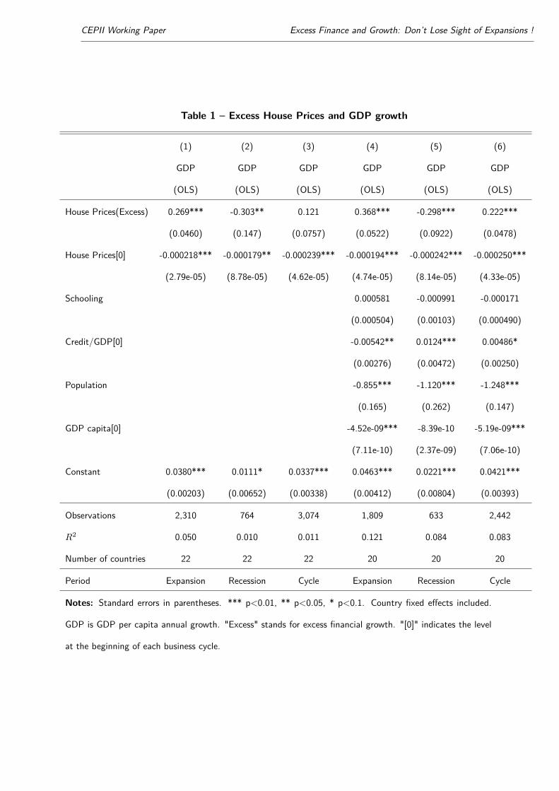
GDP growth. Table 1 shows elasticity between House Prices (Excess) and real GDP growth. We start
with no controls in the first columns and add controls moving to the right in the table. For a house
price excess of 1%, GDP increases by 0.269 points of percentage during expansions (column (1)). As
expected, the intensity of the housing boom during the expansion phase is closely associated with the
severity of the recession phase. A 1% excess in house prices growth during the expansion is associated
with a reduction of GDP growth by 0.303 points of percentage (column (2)). We control these results
using the traditional determinants of long-run growth used in the literature, among them the state of
development of the country at the beginning of each business cycle, the state of development of the
financial sector measured with the credit to GDP ratio at the beginning of each business cycle, population
growth and the average years of schooling of population aged 25 and over (see in particular Levine (1997)
or more recently Cecchetti and Kharroubi (2012)). Results confirm the positive elasticity during the
expansion and the negative elasticity during the recession (columns (4) and (5)). Excess financial growth
and economic growth move together both during expansions and recessions, but in opposite direction.
For the expansion phases, this is consistent with the well-known procyclical behaviour of finance and, for
the recession phases, it confirms the recent results reported by Drehmann et al. (2012), Claessens et al.
(2012) and Jordà et al. (2013).
Table 1 shows another interesting result on the interactions between finance and growth when it
comes to the initial condition. The coefficient of the initial value of house prices is negative for the two
20
CEPII Working Paper Excess Finance and Growth: Don’t Lose Sight of Expansions !
business cycle phases, the expansion and recession (columns (1)-(2)). This result seems in contradiction
with the literature on long-run growth which tries precisely to show that the initial state of financial
development is a good predictor for future economic growth, see Levine (1997). However, we consider
a very specific initial condition, namely the value of house prices at the end of the previous cycle, which
is the inheritance of the previous cycle. Then, starting a new cycle with a high level of house prices
is associated with a low economic growth, not only during the new expansion phase, but also during
the next recession. This effect holds even if we introduce the controls for economic growth in columns
(4)-(5). This result can be related with the concept of "Debt Supercycle" developed by Rogoff (2015)
according to which the inheritance of excessive development of finance in the past can lead to long-lasting
low economic growth (see also Lo and Rogoff (2015)). This result could also be linked to the notion of
deleveraging crisis formalized by Eggertsson and Krugman (2012). They present a new Keynesian model
of debt-driven slumps – that is, situations in which an overhang of debt on the part of some agents, who
are forced into rapid deleveraging, is depressing aggregate demand.
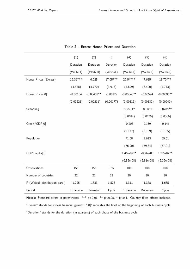
Duration. In Table 2, we employ the Weibull regression model to investigate the role of "excess finance"
as a determinant of the duration of the different phases of business cycles (Section 2.3). In line with the
literature, results of our regressions first show a positive duration dependence (P(Weibull distribution
parameter)> 1) (columns (1) to (6)), which implies that an expansion (recession) is more likely to end
the longer it lasts (see in particular Claessens et al. (2012)). We then show that large excess house prices
are associated with a longer duration of expansions (column (1)) while they are not significantly correlated
with the duration of the recession in the case of excess house prices (column (2)). These results are robust
using the controls (columns (4) and (5)). The coefficient of the initial value of house prices is negative and
significantly different from zero (column (2)) but it is no longer significant when controls are introduced
(column (5).
To our knowledge, the identification of a link between finance and expansion duration is a new
21
CEPII Working Paper Excess Finance and Growth: Don’t Lose Sight of Expansions !
Table 1 – Excess House Prices and GDP growth
(1) (2) (3) (4) (5) (6)
GDP GDP GDP GDP GDP GDP
(OLS) (OLS) (OLS) (OLS) (OLS) (OLS)
House Prices(Excess) 0.269*** -0.303** 0.121 0.368*** -0.298*** 0.222***
(0.0460) (0.147) (0.0757) (0.0522) (0.0922) (0.0478)
House Prices[0] -0.000218*** -0.000179** -0.000239*** -0.000194*** -0.000242*** -0.000250***
(2.79e-05) (8.78e-05) (4.62e-05) (4.74e-05) (8.14e-05) (4.33e-05)
Schooling 0.000581 -0.000991 -0.000171
(0.000504) (0.00103) (0.000490)
Credit/GDP[0] -0.00542** 0.0124*** 0.00486*
(0.00276) (0.00472) (0.00250)
Population -0.855*** -1.120*** -1.248***
(0.165) (0.262) (0.147)
GDP capita[0] -4.52e-09*** -8.39e-10 -5.19e-09***
(7.11e-10) (2.37e-09) (7.06e-10)
Constant 0.0380*** 0.0111* 0.0337*** 0.0463*** 0.0221*** 0.0421***
(0.00203) (0.00652) (0.00338) (0.00412) (0.00804) (0.00393)
Observations 2,310 764 3,074 1,809 633 2,442
R2 0.050 0.010 0.011 0.121 0.084 0.083
Number of countries 22 22 22 20 20 20
Period Expansion Recession Cycle Expansion Recession Cycle
Notes: Standard errors in parentheses. *** p<0.01, ** p<0.05, * p<0.1. Country fixed effects included.
GDP is GDP per capita annual growth. "Excess" stands for excess financial growth. "[0]" indicates the level
at the beginning of each business cycle.
CEPII Working Paper Excess Finance and Growth: Don’t Lose Sight of Expansions !
contribution to the literature. This result was previously suggested by Terrones et al. (2009) which show
with summary statistics that duration of the expansion is longer for business cycles with financial crisis with
no clear predictions for the economic growth. Jordà et al. (2013) suggest also with descriptive statistics
that the duration of expansion is longer for expansions with high excess credit than for expansions with
low excess credit. The literature on the links between financial cycles and business cycles do not focus on
the duration of expansions. They study recessions and recoveries. For instance, Claessens et al. (2012)
examine how the growth of asset prices prior to the recession correlates with the recession’s duration. In
their regressions, the increase in house prices prior to the recession is significantly positively related with
the recession’s duration, while equity price growth does not have a significant correlation. They do not
study the duration of expansions since the amplitude of a recovery is measured over a fixed period of four
quarters. Further research would be needed to explain the positive link between finance and expansion
duration. In Section 5, we propose alternative explanations of this correlation.
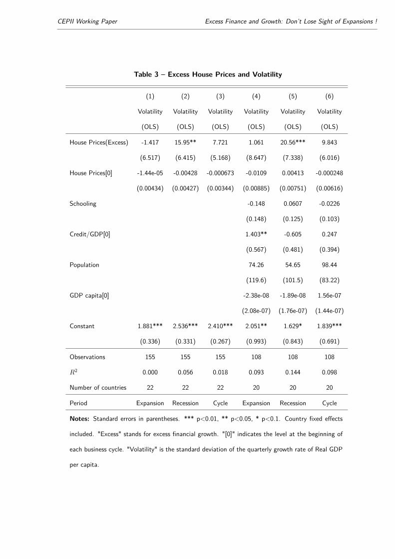
Volatility. In Table 3, we measure the links between excess house prices and the volatility of real GDP
per capita. We use as a measure of volatility the standard deviation of the quarterly growth rate of real
GDP per capita. A higher value of excess finance is associated with a higher volatility during the recession
phase (column (2)). Results during the recession phase remain significant using the controls (column
(5)). This result echoes that of Cecchetti (2008) that finds that housing booms increase the volatility
of growth. However, the absence of significant coefficients for the expansion phase for both the excess
growth and the initial value of house prices may seem surprising given the large literature devoted to
the issue of macroeconomic (in)stability associated with financial development. It is worth remembering
here that we consider the volatility of growth within business cycle phases, which is only one of the three
channels of interactions between excess finance and growth volatility, see Section 2.
It is interesting to notice that results on GDP growth, duration or volatility do not depend on the
period considered. In particular, results do not change when splitting the sample into two periods, before
23
CEPII Working Paper Excess Finance and Growth: Don’t Lose Sight of Expansions !
Table 2 – Excess House Prices and Duration
(1) (2) (3) (4) (5) (6)
Duration Duration Duration Duration Duration Duration
(Weibull) (Weibull) (Weibull) (Weibull) (Weibull) (Weibull)
House Prices (Excess) 19.39*** 6.025 17.65*** 20.54*** 7.685 18.70***
(4.588) (4.770) (3.913) (5.699) (6.400) (4.773)
House Prices[0] -0.00164 -0.00458** -0.00179 -0.00640** -0.00524 -0.00595**
(0.00223) (0.00211) (0.00177) (0.00315) (0.00332) (0.00249)
Schooling -0.0911* -0.0695 -0.0785**
(0.0484) (0.0470) (0.0366)
Credit/GDP[0] -0.208 0.139 -0.146
(0.177) (0.189) (0.135)
Population 71.08 9.613 55.01
(76.20) (59.64) (57.01)
GDP capita[0] 1.46e-07** -8.96e-08 1.22e-07**
(6.55e-08) (5.81e-08) (5.35e-08)
Observations 155 155 155 108 108 108
Number of countries 22 22 22 20 20 20
P (Weibull distribution para.) 1.225 1.333 1.528 1.311 1.368 1.685
Period Expansion Recession Cycle Expansion Recession Cycle
Notes: Standard errors in parentheses. *** p<0.01, ** p<0.05, * p<0.1. Country fixed effects included.
"Excess" stands for excess financial growth. "[0]" indicates the level at the beginning of each business cycle.
"Duration" stands for the duration (in quarters) of each phase of the business cycle.
CEPII Working Paper Excess Finance and Growth: Don’t Lose Sight of Expansions !
and after 1990 (see Table B.12 in the Appendix).
Endogeneity. The previous regressions show significant correlation between excess finance and growth
even if we control for country fixed-effects and other determinants of economic growth as originally done by
King and Levine (1993). However, as emphasized by Beck (2008), OLS estimators may not be consistent
because of the omitted variable bias, the reverse causation from growth to excess finance, and measurement
issues of variables. Instrumental Variables (IV) have been extensively used in the growth-finance literature
to overcome the biases of OLS estimators notably by instrumenting financial depth with legal origin in
cross-country analysis (Levine (1998), Levine (1999)) or by using lagged variables as internal instruments
in dynamic panel analysis (Beck et al. (2000)). In this paper, we follow the strategy recently proposed by
Arcand et al. (2015) who use an identification strategy based on the presence of heteroskedasticity in the
regression’s residual. The interest of this methodology originally developed by Rigobon (2003) and Lewbel
(2012) is to improve the identification of causal relationships even in the absence of external instruments7.
To explain the identification strategy, we follow the exposition of Lewbel (2012) and its application
in the finance-growth literature by Arcand et al. (2015). Let Y1 and Y2 be observed endogenous variables,
with Y1 the GDP growth and Y2 the excess finance, X a vector of explanatory variables, and ε = (ε1, ε2)
unobserved errors. The standard growth regression is specified as follows
Y1 = β1X + γ1Y2 + ε1 (29)
where an endogeneity issue arises because of reverse causation from growth to excess finance according
to
Y2 = β2X + γ2Y1 + ε2 (30)
7As explained by Beck (2008), the challenge with external instruments "is to identify the economic mechanisms through
which the instrumental variables influence the endogenous variable – financial development – while at the same time assuring
that the instruments are not correlated with growth directly."
25
CEPII Working Paper Excess Finance and Growth: Don’t Lose Sight of Expansions !
Table 3 – Excess House Prices and Volatility
(1) (2) (3) (4) (5) (6)
Volatility Volatility Volatility Volatility Volatility Volatility
(OLS) (OLS) (OLS) (OLS) (OLS) (OLS)
House Prices(Excess) -1.417 15.95** 7.721 1.061 20.56*** 9.843
(6.517) (6.415) (5.168) (8.647) (7.338) (6.016)
House Prices[0] -1.44e-05 -0.00428 -0.000673 -0.0109 0.00413 -0.000248
(0.00434) (0.00427) (0.00344) (0.00885) (0.00751) (0.00616)
Schooling -0.148 0.0607 -0.0226
(0.148) (0.125) (0.103)
Credit/GDP[0] 1.403** -0.605 0.247
(0.567) (0.481) (0.394)
Population 74.26 54.65 98.44
(119.6) (101.5) (83.22)
GDP capita[0] -2.38e-08 -1.89e-08 1.56e-07
(2.08e-07) (1.76e-07) (1.44e-07)
Constant 1.881*** 2.536*** 2.410*** 2.051** 1.629* 1.839***
(0.336) (0.331) (0.267) (0.993) (0.843) (0.691)
Observations 155 155 155 108 108 108
R2 0.000 0.056 0.018 0.093 0.144 0.098
Number of countries 22 22 22 20 20 20
Period Expansion Recession Cycle Expansion Recession Cycle
Notes: Standard errors in parentheses. *** p<0.01, ** p<0.05, * p<0.1. Country fixed effects
included. "Excess" stands for excess financial growth. "[0]" indicates the level at the beginning of
each business cycle. "Volatility" is the standard deviation of the quarterly growth rate of Real GDP
per capita.
CEPII Working Paper Excess Finance and Growth: Don’t Lose Sight of Expansions !
The exogenous regressors X should satisfy here the minimal assumption that E (εX) = 0. Lewbel (2012)
demonstrated that the structural model parameters, namely the β, remain unidentified under the standard
homoskedasticity assumption that E (εε′|X) is constant. However, the structural model parameters
may be identified given some heteroskedasticity, in particular if cov(X, ε2
j
)6= 0, for j = 1, 2, and
cov (Z, ε1ε2) 6= 0 for an observed Z, where Z can be a subset of X. Arcand et al. (2015) suggest to use
Xε2 as an instrument for Y2.8
Table 4 reports the estimates of the models of Tables 1 (columns (4), (5), and (6)) and 3 (columns
(4), (5), (6)) using identification through heteroskedasticity (Rigobon (2003), Lewbel (2012))9. As in
the OLS estimations of Table 1, we find a positive relationship between House Prices (Excess) and GDP
growth during the expansion (column (1)) and a negative one during the recession (column (2)). As
in Table 3, we find that a higher value of excess finance is associated with a higher volatility during
the recession phase (column (5)). The coefficients associated with House Prices (Excess) are precisely
estimated, suggesting that cov (X, ε22) is not close to zero and the Hansen’s J test fails to reject the
overidentifying restrictions at the 5% confidence level.
4.2. Growth Cycle Accounting
Regression results show several interactions between excess finance and the characteristics of the expan-
sions and recessions, namely their growth rates, durations, and volatilities. This section uses the growth
cycle accounting procedure to determine the implications of these interactions on the long-run economic
growth and volatility. To do so, we apply the formulas presented in Section 2 for the estimates of the
coefficients αphx which are significantly different form zero at the 10% level, otherwise the zero value is
8This is a good instrument because the assumption that cov(X, ε1ε2) = 0 guarantees that Xε2 is uncorrelated with ε1,
and the presence of heteroskedasticity (cov(X, ε22) 6= 0) guarantees that Xε2 is correlated with ε2 and thus with Y2. Using
the stata function ivreg2h.do, we use the instrument (Z − E (Z)) ε2 as originally suggested by Lewbel (2012).9We cannot use the same methodology for the Weibull regression model we use in Table 2. In this section, we thus choose
to focus on controlling the endogeneity of the OLS regressions.
27
CEPII Working Paper Excess Finance and Growth: Don’t Lose Sight of Expansions !
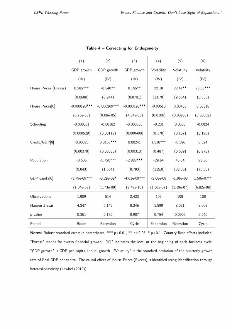
Table 4 – Correcting for Endogeneity
(1) (2) (3) (4) (5) (6)
GDP growth GDP growth GDP growth Volatility Volatility Volatility
(IV) (IV) (IV) (IV) (IV) (IV)
House Prices (Excess) 0.285*** -0.540** 0.155** 22.10 22.41** 25.05***
(0.0608) (0.244) (0.0701) (13.79) (9.564) (8.835)
House Prices[0] -0.000190*** -0.000269*** -0.000198*** -0.00613 0.00455 0.00318
(5.76e-05) (9.08e-05) (4.84e-05) (0.0106) (0.00953) (0.00682)
Schooling -0.000351 -0.00182 -0.000533 -0.231 0.0535 -0.0824
(0.000529) (0.00112) (0.000480) (0.170) (0.137) (0.120)
Credit/GDP[0] -0.00323 0.0150*** 0.00241 1.510*** -0.596 0.324
(0.00378) (0.00535) (0.00313) (0.487) (0.689) (0.278)
Population -0.606 -5.720*** -2.888*** -29.64 45.54 23.36
(0.843) (1.564) (0.793) (115.0) (82.33) (78.55)
GDP capita[0] -3.79e-09*** -3.29e-09* -4.63e-09*** -2.08e-08 -1.86e-08 1.58e-07**
(1.04e-09) (1.73e-09) (9.49e-10) (1.02e-07) (1.19e-07) (6.82e-08)
Observations 1,909 514 2,423 108 108 108
Hansen J Stat. 4.347 6.145 0.346 1.899 8.031 3.068
p-value 0.361 0.189 0.987 0.754 0.0905 0.546
Period Boom Recession Cycle Expansion Recession Cycle
Notes: Robust standard errors in parentheses. *** p<0.01, ** p<0.05, * p<0.1. Country fixed effects included.
"Excess" stands for excess financial growth. "[0]" indicates the level at the beginning of each business cycle.
"GDP growth" is GDP per capita annual growth. "Volatility" is the standard deviation of the quarterly growth
rate of Real GDP per capita. The causal effect of House Prices (Excess) is identified using identification through
heteroskedasticity (Lewbel (2012)).
CEPII Working Paper Excess Finance and Growth: Don’t Lose Sight of Expansions !
imposed, where ph = {ex, re} and x = {g, T, sd}.
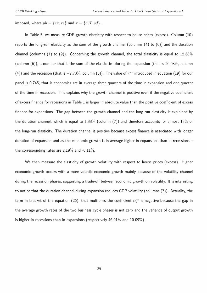
In Table 5, we measure GDP growth elasticity with respect to house prices (excess). Column (10)
reports the long-run elasticity as the sum of the growth channel (columns (4) to (6)) and the duration
channel (columns (7) to (9)). Concerning the growth channel, the total elasticity is equal to 12.38%
(column (6)), a number that is the sum of the elasticities during the expansion (that is 20.08%, column
(4)) and the recession (that is −7.70%, column (5)). The value of π̃ex introduced in equation (19) for our
panel is 0.745, that is economies are in average three quarters of the time in expansion and one quarter
of the time in recession. This explains why the growth channel is positive even if the negative coefficient
of excess finance for recessions in Table 1 is larger in absolute value than the positive coefficient of excess
finance for expansions. The gap between the growth channel and the long-run elasticity is explained by
the duration channel, which is equal to 1.88% (column (7)) and therefore accounts for almost 13% of
the long-run elasticity. The duration channel is positive because excess finance is associated with longer
duration of expansion and as the economic growth is in average higher in expansions than in recessions –
the corresponding rates are 2.19% and -0.11%.
We then measure the elasticity of growth volatility with respect to house prices (excess). Higher
economic growth occurs with a more volatile economic growth mainly because of the volatility channel
during the recession phases, suggesting a trade-off between economic growth on volatility. It is interesting
to notice that the duration channel during expansion reduces GDP volatility (columns (7)). Actuallty, the
term in bracket of the equation (26), that multiplies the coefficient αexτ is negative because the gap in
the average growth rates of the two business cycle phases is not zero and the variance of output growth
is higher in recessions than in expansions (respectively 46.91% and 10.09%).
29
CEPII Working Paper Excess Finance and Growth: Don’t Lose Sight of Expansions !
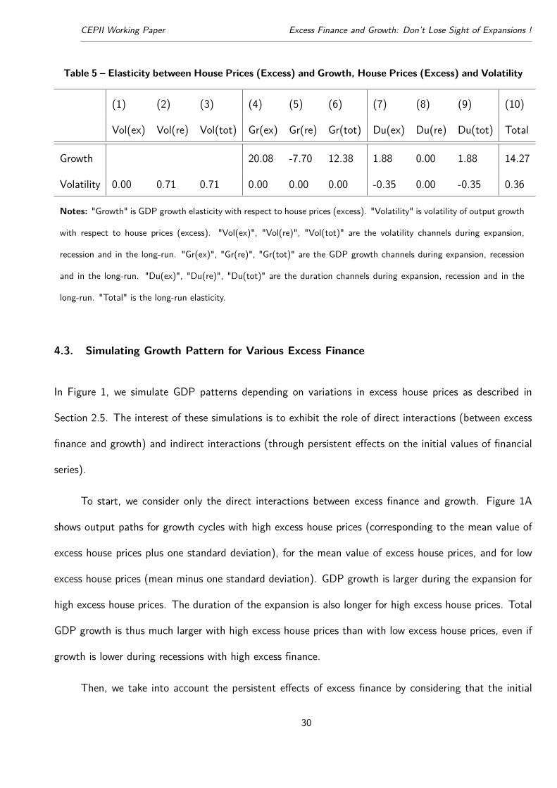
Table 5 – Elasticity between House Prices (Excess) and Growth, House Prices (Excess) and Volatility
(1) (2) (3) (4) (5) (6) (7) (8) (9) (10)
Vol(ex) Vol(re) Vol(tot) Gr(ex) Gr(re) Gr(tot) Du(ex) Du(re) Du(tot) Total
Growth 20.08 -7.70 12.38 1.88 0.00 1.88 14.27
Volatility 0.00 0.71 0.71 0.00 0.00 0.00 -0.35 0.00 -0.35 0.36
Notes: "Growth" is GDP growth elasticity with respect to house prices (excess). "Volatility" is volatility of output growth
with respect to house prices (excess). "Vol(ex)", "Vol(re)", "Vol(tot)" are the volatility channels during expansion,
recession and in the long-run. "Gr(ex)", "Gr(re)", "Gr(tot)" are the GDP growth channels during expansion, recession
and in the long-run. "Du(ex)", "Du(re)", "Du(tot)" are the duration channels during expansion, recession and in the
long-run. "Total" is the long-run elasticity.
4.3. Simulating Growth Pattern for Various Excess Finance
In Figure 1, we simulate GDP patterns depending on variations in excess house prices as described in
Section 2.5. The interest of these simulations is to exhibit the role of direct interactions (between excess
finance and growth) and indirect interactions (through persistent effects on the initial values of financial
series).
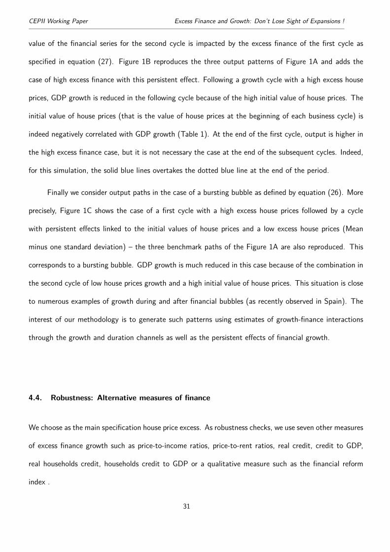
To start, we consider only the direct interactions between excess finance and growth. Figure 1A
shows output paths for growth cycles with high excess house prices (corresponding to the mean value of
excess house prices plus one standard deviation), for the mean value of excess house prices, and for low
excess house prices (mean minus one standard deviation). GDP growth is larger during the expansion for
high excess house prices. The duration of the expansion is also longer for high excess house prices. Total
GDP growth is thus much larger with high excess house prices than with low excess house prices, even if
growth is lower during recessions with high excess finance.
Then, we take into account the persistent effects of excess finance by considering that the initial
30
CEPII Working Paper Excess Finance and Growth: Don’t Lose Sight of Expansions !
value of the financial series for the second cycle is impacted by the excess finance of the first cycle as
specified in equation (27). Figure 1B reproduces the three output patterns of Figure 1A and adds the
case of high excess finance with this persistent effect. Following a growth cycle with a high excess house
prices, GDP growth is reduced in the following cycle because of the high initial value of house prices. The
initial value of house prices (that is the value of house prices at the beginning of each business cycle) is
indeed negatively correlated with GDP growth (Table 1). At the end of the first cycle, output is higher in
the high excess finance case, but it is not necessary the case at the end of the subsequent cycles. Indeed,
for this simulation, the solid blue lines overtakes the dotted blue line at the end of the period.
Finally we consider output paths in the case of a bursting bubble as defined by equation (26). More
precisely, Figure 1C shows the case of a first cycle with a high excess house prices followed by a cycle
with persistent effects linked to the initial values of house prices and a low excess house prices (Mean
minus one standard deviation) – the three benchmark paths of the Figure 1A are also reproduced. This
corresponds to a bursting bubble. GDP growth is much reduced in this case because of the combination in
the second cycle of low house prices growth and a high initial value of house prices. This situation is close
to numerous examples of growth during and after financial bubbles (as recently observed in Spain). The
interest of our methodology is to generate such patterns using estimates of growth-finance interactions
through the growth and duration channels as well as the persistent effects of financial growth.
4.4. Robustness: Alternative measures of finance
We choose as the main specification house price excess. As robustness checks, we use seven other measures
of excess finance growth such as price-to-income ratios, price-to-rent ratios, real credit, credit to GDP,
real households credit, households credit to GDP or a qualitative measure such as the financial reform
index .
31

CEPII Working Paper Excess Finance and Growth: Don’t Lose Sight of Expansions !
Figure 1 – SIMULATION OF OUTPUT PATHS FOR VARIATIONS IN EXCESS HOUSE PRICES
0.5
11.
5
0 20 40 60 80
Mean(M) M+1sdM-1sd
(A) Output Paths for +/- one SD of House Prices
0.2
.4.6
.81
0 10 20 30 40 50
Mean(M) M+1sdM+1sd(C1),+persistence(C2) M-1sd
(B) Output Paths with Hysteresis
0.2
.4.6
.81
0 10 20 30 40 50
Mean(M) M+1sdM+1sd(C1),M-1sd+persistence(C2) M-1sd
(C) Output Paths with Hysteresis and Bursting Bubble
Notes: Figure 1A shows output paths for business cycles with high excess house prices (corresponding to the mean
value of excess house prices plus one standard deviation ("M+1sd", in blue), for the mean value of excess house
prices ("M", in black), and for low excess house prices (mean minus one standard deviation, in red). Figure 1B
reproduces the three output patterns of Figure 1A and adds the case of high excess finance with a persistent effect
in cycle 2 ("C2", Blue dash-line). Figure 1C shows the case of a first cycle ("C1") with a high excess house prices
followed by a cycle with persistent effects on the initial values of house prices and a low excess house prices (Mean
minus one standard deviation, "M-1sd+persistence(C2)", Blue dash-line) – the three benchmark paths of the Figure
1A are also reproduced. We show coefficients that are significantly different form zero at the 10% level, otherwise
the zero value is imposed.
CEPII Working Paper Excess Finance and Growth: Don’t Lose Sight of Expansions !
Regression results for seven alternative measures. The correlation between excess dinance and
GDP growth is very robust in expansion and recession for the seven alternative measures. Price-to-income
ratios (excess), price-to-rent ratios (excess), real credit (excess), credit to GDP (excess), real households
credit (excess), households credit to GDP (excess) and the financial reform index are all associated with
higher GDP growth during the expansion and lower growth during the recession (columns (1) and (2) of
Tables B.3, B.4, B.5, B.6, B.7, B.8, B.9).
Concerning duration, the seven different measures of excess finance growth indicate a strongly
positive and significant correlation between excess finance growth and the duration of the expansion
phase (columns (3) of Tables B.3, B.4, B.5, B.6, B.7, B.8, B.9). We find also a positive and significant
correlation between excess finance growth and the duration of the recession in the case of the price-to-
income ratios and credit to GDP (column (9) of Tables B.3 and B.6).
Concerning volatility, there is positive and significant correlation between excess finance and the
volatility of recession in the cases of price-to-income ratios, price-to-rent ratios, real credit and the financial
reform index (column (6) of Tables B.3, B.4, B.5, B.9). The regression is not significant in the case of
expansion (column (5) of B.3, B.4, B.5, B.9), except for credit to GDP, real households credit and
households credit to GDP where we find a negative correlation between excess finance and volatility
(column (5) of Tables B.6, B.7, B.8).
Growth Cycle Accounting for seven other measures. In Table B.10, we compute GDP growth
elasticity with respect to the eight measures of excess finance growth. Column (10) reports the long-run
elasticity as the sum of the growth channel (columns (4) to (6)) and the duration channel (columns (7)
to (9)). For seven out of the eight measures of excess finance, the long-run elasticity is positive. This
is the case for house prices, price-to income ratio, price-to-rent ratio, real credit, real households credit,
households credit to GDP and Financial reforms (the only exception is credit to GDP). For these seven
33
CEPII Working Paper Excess Finance and Growth: Don’t Lose Sight of Expansions !
measures, the elasticity for the growth channel during the expansion phases is positive, with a number
higher than the economic growth during the recession phase. The growth channel, defined as the sum of
these two elasticities, is equal to 12% for house prices, 20% for the price-to-income ratio, 19% for the
price-to-rent ratio, 18% for real credit, 16% for real households credit, 11% for households credit to GDP.
Concerning the duration channel, the elasticity is positive for all the measures of excess finance, with a
range of results going from 0.4% (financial reforms) to 3.3% (real credit). The total long-run elasticity is
positive for all the measures, except credit to GDP.
In Table B.11, we compute GDP volatility elasticity with respect to the eight measures of excess
finance growth. Contrary to GDP growth, the sign of the total elasticity depends on the measure consid-
ered. For house prices and real credit, total elasticity is positive. For the six other measures, this elasticity
is negative. It is thus not possible to conclude that higher economic growth occurs with a more volatile
economic growth.
Simulations of Growth Patterns. We simulate the patterns of output growth for various values of
excess finance using the estimation results for real credit, and households credit (see Figures A.1, A.2 and
A.3). The properties exhibited for house prices are shared with these financial series. Indeed, as for house
prices, a high value of excess finance is associated with higher growth in longer expansions during the first
cycle but growth may be reduced in the subsequent cycle if one considers persistent effects and bubble
burst (eg negative excess finance).
5. Concluding Remarks
We propose in this paper a new accounting procedure to study the interactions between excess financial
growth and economic growth. We show that the finance-growth elasticity in the long-run can be viewed as
the cumulative of finance-growth interactions within each cycle through a growth channel and a duration
channel. Our empirical analysis delivers three key properties of the interactions between finance and
34
CEPII Working Paper Excess Finance and Growth: Don’t Lose Sight of Expansions !
growth.
1. Recessions are more severe after episodes of high excess finance.
2. High excess finance occurs with a high output growth rate during a long expansion phase.
3. High initial value of financial series at the beginning of a cycle is associated with a low output growth
during the expansion and recession of this cycle.
The first property is nowadays well-known and constitutes the focus of the literature on finance and
growth, see in particular Drehmann et al. (2012), Claessens et al. (2012) and Jordà et al. (2013). The third
property is also of importance since it can be related with the concept of "Debt Supercycle" developed
by Rogoff (2015) according to which the inheritance of excessive development of finance in the past can
lead to long-lasting low economic growth. This result could also be linked to the notion of deleveraging
crisis formalized by Eggertsson and Krugman (2012). Concerning the second property, the identification
of a link between finance and expansion duration is a new contribution to the literature. It is interesting
to notice that this property suggests a different pattern from the one described by Ranciere et al. (2008)
in which financial liberalization leads to higher long-run growth but also to more crises, implying shorter
expansions. In our paper, high excess finance is accompanied by a longer duration of expansions. Several
mechanisms could explain this property. A first interpretation could be based on the procyclical behaviour
of finance as stated by the financial accelerator mechanism developed by Bernanke et al. (1999). Indeed,
an improvement of the fundamentals of the economic leads to more both growth and financial activities.
A second interpretation could be based on the "time is different" syndrome developed by Reinhart and
Rogoff (2008). A long expansion may be a favorable context for the development of beliefs at the origin of
excessive developments of financial activities. A third interpretation could be that bubbles in the expansion
phase can play as a shock absorber. An oil shock could be for example more easily absorbed in a country
when growth is fed by a bubble. Hence, we conclude that further research would be needed to investigate
the links between the duration of expansion and excess finance, in particular the sense of causality and
35

CEPII Working Paper Excess Finance and Growth: Don’t Lose Sight of Expansions !
economic mechanisms behind the relationship.
36
CEPII Working Paper Excess Finance and Growth: Don’t Lose Sight of Expansions !
References
Arcand, J.-L., Berkes, E., and Panizza, U. (2015). Too much finance? Journal of Economic Growth,
Volume 20(Issue 2).
Beck, T. (2008). The econometrics of finance and growth, volume 4608. World Bank Publications.
Beck, T., Levine, R., and Loayza, N. (2000). Finance and the sources of growth àňİ. 58.
Bernanke, B. S., Gertler, M., and Gilchrist, S. (1999). The financial accelerator in a quantitative business
cycle framework. Handbook of macroeconomics, 1:1341–1393.
Blanchard, O., Cerutti, E., and Summers, L. (2015). Inflation and Activity–Two Explorations and their
Monetary Policy Implications. Technical report, National Bureau of Economic Research.
Bonfiglioli, A. (2008). Financial integration, productivity and capital accumulation. Journal of International
Economics, 76(2):337–355.
Borio, C., Disyatat, P., and Juselius, M. (2013). Rethinking potential output : Embedding information
about the financial cycle. (404).
Bry, G. and Boschan, C. (1971). Programmed selection of cyclical turning points. In Cyclical Analysis of
Time Series: Selected Procedures and Computer Programs, pages 7–63. UMI.
Cecchetti, S. G. (2008). Measuring the macroeconomic risks posed by asset price booms. In Asset prices
and monetary policy, pages 9–43. University of Chicago Press.
Cecchetti, S. G. and Kharroubi, E. (2012). Reassessing the impact of finance on growth. (381).
Claessens, S., Kose, M. A., and Terrones, M. E. (2012). How do business and financial cycles interact?
Journal of International Economics, 87(1):178–190.
Drehmann, M., Borio, C. E. V., and Tsatsaronis, K. (2012). Characterising the financial cycle: don’t lose
sight of the medium term!
Eggertsson, G. B. and Krugman, P. (2012). Debt, deleveraging, and the liquidity trap: A fisher-minsky-koo
37
CEPII Working Paper Excess Finance and Growth: Don’t Lose Sight of Expansions !
approach*. The Quarterly Journal of Economics, page qjs023.
Gadea Rivas, M. D. and Perez-Quiros, G. (2015). the Failure To Predict the Great Recession-a View
Through the Role of Credit. Journal of the European Economic Association, 13(3):534–559.
Galí, J. (2015). Insider Outsider Labor Markets, Hysteresis and Monetary Policy. CREI, U P F Barcelona,
G S E.
Goldsmith, R. (1969). Financial structure and economic development. New Haven: Yale University Pres.
Harding, D. and Pagan, A. (2002). Dissecting the cycle: a methodological investigation. Journal of
monetary economics, 49(2):365–381.
Jordà, O., Schularick, M., and Taylor, A. M. (2014). The great mortgaging: Housing finance, crises, and
business cycles. Technical report, National Bureau of Economic Research.
Jordà, O., Schularick, M. H. P., and Taylor, A. M. (2013). Sovereigns versus Banks: Credit, Crises, and
Consequences. Technical report, National Bureau of Economic Research.
King, R. G. and Levine, R. (1993). Finance and growth: Schumpeter might be right. The Quarterly
Journal of Economics, 108(3):717–737.
Krugman, P. (2013). Secular Stagnation, Coalmines, Bubbles, and Larry Summers. New York Times,
(November 16), pages 1–6.
Levine, R. (1997). Economic Development and Financial and Agenda Growth: Views and Agenda. Jel,
35(2):688–726.
Levine, R. (1998). The legal environment, banks, and long-run economic growth. Journal of money, credit
and banking, pages 596–613.
Levine, R. (1999). Law, finance, and economic growth. Journal of financial Intermediation, 8(1):8–35.
Lewbel, A. (2012). Using heteroscedasticity to identify and estimate mismeasured and endogenous re-
gressor models. Journal of Business & Economic Statistics, 30(1):67–80.
38
CEPII Working Paper Excess Finance and Growth: Don’t Lose Sight of Expansions !
Lo, S. H. and Rogoff, K. (2015). Secular stagnation, debt overhang and other rationales for sluggish
growth, six years on. BIS Working Paper 482.
McKinnon, R. I. (1973). Money and capital in economic development. Brookings Institution Press.
Rancière, R. and Tornell, A. (2015). Financial Liberalization, Debt Mismatch, Allocative Efficiency and
Growth. American Economic Journal: Macroeconomics, forthcomin.
Ranciere, R., Tornell, A., and Westermann, F. (2006). Decomposing the effects of financial liberalization:
Crises vs. growth. Journal of Banking and Finance, 30(12):3331–3348.
Ranciere, R., Tornell, A., and Westermann, F. (2008). Systemic crises and growth. The Quarterly Journal
of Economics, 123(1):359–406.
Reinhart, C. M. and Rogoff, K. (2008). This time is different: Eight centuries of financial folly. Princeton
Univ Pr.
Rigobon, R. (2003). Identification through heteroskedasticity. Review of Economics and Statistics,
85(4):777–792.
Rogoff, K. (2015). Debt supercycle, not secular stagnation. Vox: CEPRâĂŹs Policy Portal.
Rousseau, P. L. and Wachtel, P. (2011). What is happening to the impact of financial deepening on
economic growth? Economic Inquiry, 49(1):276–288.
Rousseau, P. L. and Wachtel, P. (2015). Episodes of Financial Deepening: Credit Booms or Growth
Generators? Peter L. Rousseau and Paul Wachtel March 2015. (March):1–27.
Schularick, M. and Taylor, A. M. (2012). Credit Booms Gone Bust: Monetary Policy, Leverage Cycles,
and Financial Crises, 1870-2008. The American Economic Review, 102(2):1029–1061.
Summers, L. (2013). Why stagnation might prove to be the new normal. The Financial Times, December
1.
Summers, L. H. (2015). Reflections on Secular Stagnation.
39

CEPII Working Paper Excess Finance and Growth: Don’t Lose Sight of Expansions !
Terrones, M. E., Scott, A., Kannan, P., and Others (2009). From recession to recovery: How soon and
how strong? International Monetary Fund, World Economic Outlook, April.
40

CEPII Working Paper Excess Finance and Growth: Don’t Lose Sight of Expansions !
Appendix
A. Figures
41
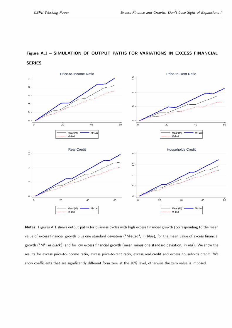
CEPII Working Paper Excess Finance and Growth: Don’t Lose Sight of Expansions !
Figure A.1 – SIMULATION OF OUTPUT PATHS FOR VARIATIONS IN EXCESS FINANCIAL
SERIES
0.2
.4.6
.81
0 20 40 60
Mean(M) M+1sdM-1sd
Price-to-Income Ratio
0.5
11.
5
0 20 40 60
Mean(M) M+1sdM-1sd
Price-to-Rent Ratio
0.5
11.
5
0 20 40 60
Mean(M) M+1sdM-1sd
Real Credit
0.5
11.
52
0 20 40 60 80
Mean(M) M+1sdM-1sd
Households Credit
Notes: Figures A.1 shows output paths for business cycles with high excess financial growth (corresponding to the mean
value of excess financial growth plus one standard deviation ("M+1sd", in blue), for the mean value of excess financial
growth ("M", in black), and for low excess financial growth (mean minus one standard deviation, in red). We show the
results for excess price-to-income ratio, excess price-to-rent ratio, excess real credit and excess households credit. We
show coefficients that are significantly different form zero at the 10% level, otherwise the zero value is imposed.
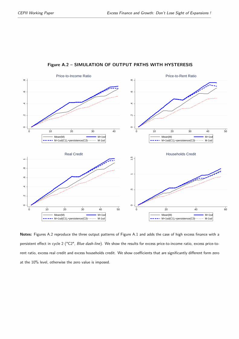
CEPII Working Paper Excess Finance and Growth: Don’t Lose Sight of Expansions !
Figure A.2 – SIMULATION OF OUTPUT PATHS WITH HYSTERESIS
0.2
.4.6
.8
0 10 20 30 40
Mean(M) M+1sdM+1sd(C1),+persistence(C2) M-1sd
Price-to-Income Ratio
0.2
.4.6
.80 10 20 30 40 50
Mean(M) M+1sdM+1sd(C1),+persistence(C2) M-1sd
Price-to-Rent Ratio
0.2
.4.6
.81
0 10 20 30 40 50
Mean(M) M+1sdM+1sd(C1),+persistence(C2) M-1sd
Real Credit
0.5
11.
5
0 20 40 60
Mean(M) M+1sdM+1sd(C1),+persistence(C2) M-1sd
Households Credit
Notes: Figures A.2 reproduce the three output patterns of Figure A.1 and adds the case of high excess finance with a
persistent effect in cycle 2 ("C2", Blue dash-line). We show the results for excess price-to-income ratio, excess price-to-
rent ratio, excess real credit and excess households credit. We show coefficients that are significantly different form zero
at the 10% level, otherwise the zero value is imposed.
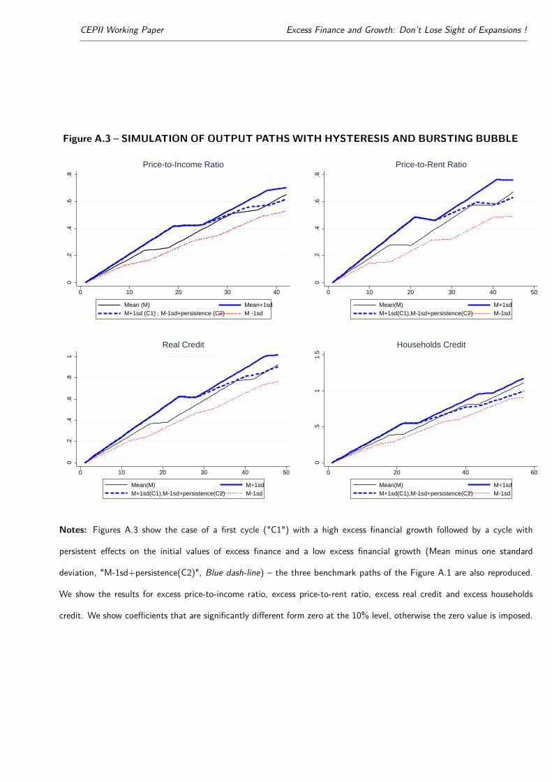
CEPII Working Paper Excess Finance and Growth: Don’t Lose Sight of Expansions !
Figure A.3 – SIMULATION OF OUTPUT PATHS WITH HYSTERESIS AND BURSTING BUBBLE
0.2
.4.6
.8
0 10 20 30 40
Mean (M) Mean+1sdM+1sd (C1) ; M-1sd+persistence (C2) M -1sd
Price-to-Income Ratio
0.2
.4.6
.8
0 10 20 30 40 50
Mean(M) M+1sdM+1sd(C1),M-1sd+persistence(C2) M-1sd
Price-to-Rent Ratio
0.2
.4.6
.81
0 10 20 30 40 50
Mean(M) M+1sdM+1sd(C1),M-1sd+persistence(C2) M-1sd
Real Credit
0.5
11.
5
0 20 40 60
Mean(M) M+1sdM+1sd(C1),M-1sd+persistence(C2) M-1sd
Households Credit
Notes: Figures A.3 show the case of a first cycle ("C1") with a high excess financial growth followed by a cycle with
persistent effects on the initial values of excess finance and a low excess financial growth (Mean minus one standard
deviation, "M-1sd+persistence(C2)", Blue dash-line) – the three benchmark paths of the Figure A.1 are also reproduced.
We show the results for excess price-to-income ratio, excess price-to-rent ratio, excess real credit and excess households
credit. We show coefficients that are significantly different form zero at the 10% level, otherwise the zero value is imposed.
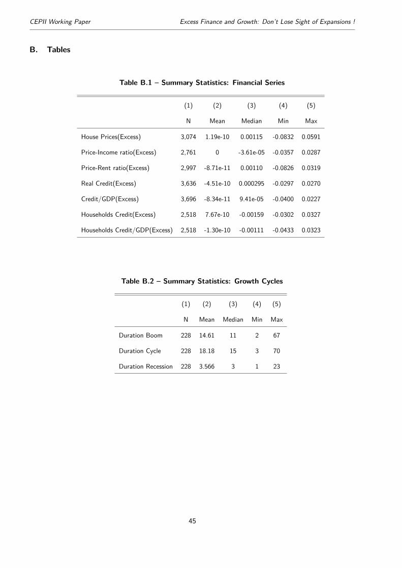
CEPII Working Paper Excess Finance and Growth: Don’t Lose Sight of Expansions !
B. Tables
Table B.1 – Summary Statistics: Financial Series
(1) (2) (3) (4) (5)
N Mean Median Min Max
House Prices(Excess) 3,074 1.19e-10 0.00115 -0.0832 0.0591
Price-Income ratio(Excess) 2,761 0 -3.61e-05 -0.0357 0.0287
Price-Rent ratio(Excess) 2,997 -8.71e-11 0.00110 -0.0826 0.0319
Real Credit(Excess) 3,636 -4.51e-10 0.000295 -0.0297 0.0270
Credit/GDP(Excess) 3,696 -8.34e-11 9.41e-05 -0.0400 0.0227
Households Credit(Excess) 2,518 7.67e-10 -0.00159 -0.0302 0.0327
Households Credit/GDP(Excess) 2,518 -1.30e-10 -0.00111 -0.0433 0.0323
Table B.2 – Summary Statistics: Growth Cycles
(1) (2) (3) (4) (5)
N Mean Median Min Max
Duration Boom 228 14.61 11 2 67
Duration Cycle 228 18.18 15 3 70
Duration Recession 228 3.566 3 1 23
45
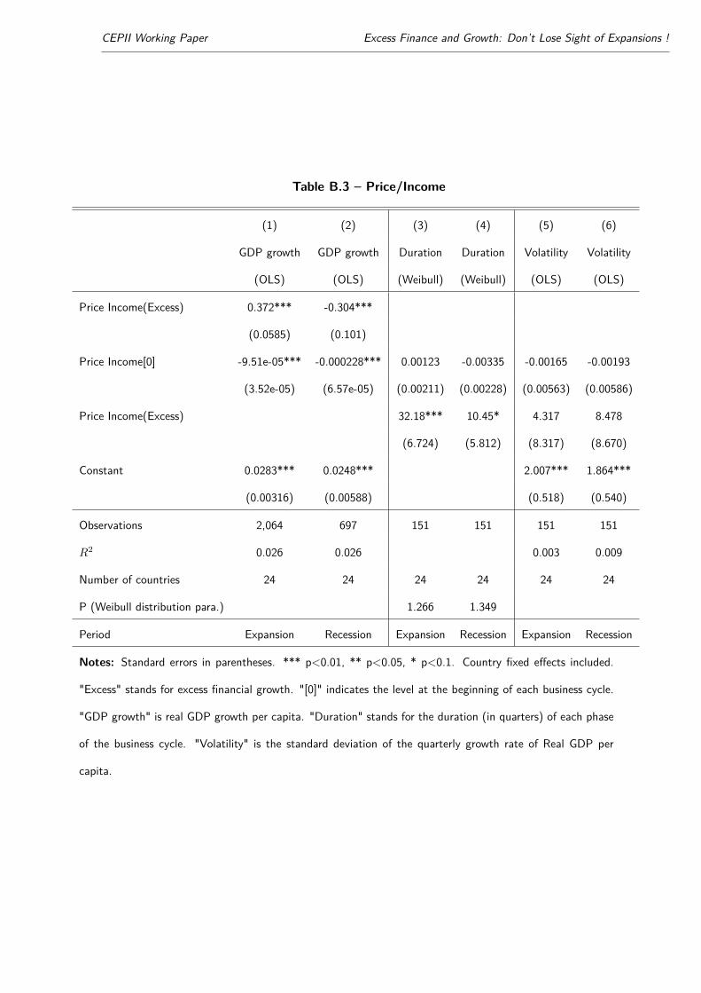
CEPII Working Paper Excess Finance and Growth: Don’t Lose Sight of Expansions !
Table B.3 – Price/Income
(1) (2) (3) (4) (5) (6)
GDP growth GDP growth Duration Duration Volatility Volatility
(OLS) (OLS) (Weibull) (Weibull) (OLS) (OLS)
Price Income(Excess) 0.372*** -0.304***
(0.0585) (0.101)
Price Income[0] -9.51e-05*** -0.000228*** 0.00123 -0.00335 -0.00165 -0.00193
(3.52e-05) (6.57e-05) (0.00211) (0.00228) (0.00563) (0.00586)
Price Income(Excess) 32.18*** 10.45* 4.317 8.478
(6.724) (5.812) (8.317) (8.670)
Constant 0.0283*** 0.0248*** 2.007*** 1.864***
(0.00316) (0.00588) (0.518) (0.540)
Observations 2,064 697 151 151 151 151
R2 0.026 0.026 0.003 0.009
Number of countries 24 24 24 24 24 24
P (Weibull distribution para.) 1.266 1.349
Period Expansion Recession Expansion Recession Expansion Recession
Notes: Standard errors in parentheses. *** p<0.01, ** p<0.05, * p<0.1. Country fixed effects included.
"Excess" stands for excess financial growth. "[0]" indicates the level at the beginning of each business cycle.
"GDP growth" is real GDP growth per capita. "Duration" stands for the duration (in quarters) of each phase
of the business cycle. "Volatility" is the standard deviation of the quarterly growth rate of Real GDP per
capita.
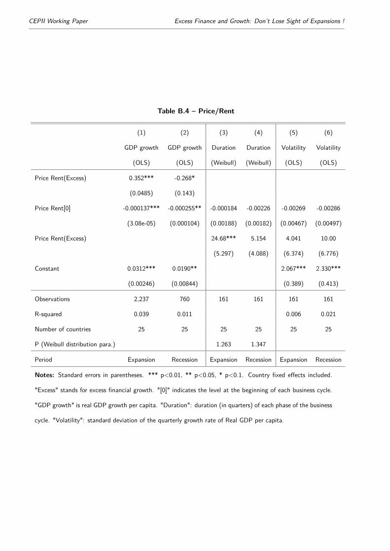
CEPII Working Paper Excess Finance and Growth: Don’t Lose Sight of Expansions !
Table B.4 – Price/Rent
(1) (2) (3) (4) (5) (6)
GDP growth GDP growth Duration Duration Volatility Volatility
(OLS) (OLS) (Weibull) (Weibull) (OLS) (OLS)
Price Rent(Excess) 0.352*** -0.268*
(0.0485) (0.143)
Price Rent[0] -0.000137*** -0.000255** -0.000184 -0.00226 -0.00269 -0.00286
(3.08e-05) (0.000104) (0.00188) (0.00182) (0.00467) (0.00497)
Price Rent(Excess) 24.68*** 5.154 4.041 10.00
(5.297) (4.088) (6.374) (6.776)
Constant 0.0312*** 0.0190** 2.067*** 2.330***
(0.00246) (0.00844) (0.389) (0.413)
Observations 2,237 760 161 161 161 161
R-squared 0.039 0.011 0.006 0.021
Number of countries 25 25 25 25 25 25
P (Weibull distribution para.) 1.263 1.347
Period Expansion Recession Expansion Recession Expansion Recession
Notes: Standard errors in parentheses. *** p<0.01, ** p<0.05, * p<0.1. Country fixed effects included.
"Excess" stands for excess financial growth. "[0]" indicates the level at the beginning of each business cycle.
"GDP growth" is real GDP growth per capita. "Duration": duration (in quarters) of each phase of the business
cycle. "Volatility": standard deviation of the quarterly growth rate of Real GDP per capita.
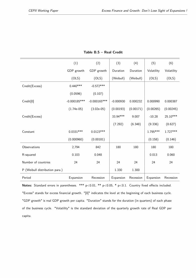
CEPII Working Paper Excess Finance and Growth: Don’t Lose Sight of Expansions !
Table B.5 – Real Credit
(1) (2) (3) (4) (5) (6)
GDP growth GDP growth Duration Duration Volatility Volatility
(OLS) (OLS) (Weibull) (Weibull) (OLS) (OLS)
Credit(Excess) 0.440*** -0.572***
(0.0596) (0.107)
Credit[0] -0.000185*** -0.000165*** -0.000930 0.000232 0.000990 0.000387
(1.74e-05) (3.02e-05) (0.00193) (0.00171) (0.00265) (0.00245)
Credit(Excess) 33.94*** 9.007 -10.28 25.10***
(7.292) (6.348) (9.336) (8.627)
Constant 0.0331*** 0.0123*** 1.795*** 1.727***
(0.000960) (0.00181) (0.158) (0.146)
Observations 2,794 842 180 180 180 180
R-squared 0.103 0.048 0.013 0.060
Number of countries 24 24 24 24 24 24
P (Weibull distribution para.) 1.330 1.300
Period Expansion Recession Expansion Recession Expansion Recession
Notes: Standard errors in parentheses. *** p<0.01, ** p<0.05, * p<0.1. Country fixed effects included.
"Excess" stands for excess financial growth. "[0]" indicates the level at the beginning of each business cycle.
"GDP growth" is real GDP growth per capita. "Duration" stands for the duration (in quarters) of each phase
of the business cycle. "Volatility" is the standard deviation of the quarterly growth rate of Real GDP per
capita.

CEPII Working Paper Excess Finance and Growth: Don’t Lose Sight of Expansions !
Table B.6 – Credit/GDP
(1) (2) (3) (4) (5) (6)
GDP growth GDP growth Duration Duration Volatility Volatility
(OLS) (OLS) (Weibull) (Weibull) (OLS) (OLS)
Credit/GDP(Excess) 0.136** -0.714***
(0.0646) (0.108)
Credit/GDP[0] -0.0157*** -0.0113*** 0.00179 0.0200 0.211 -0.121
(0.00133) (0.00230) (0.119) (0.0957) (0.205) (0.198)
Credit/GDP(Excess) 38.46*** 12.70** -17.94* 14.71*
(7.077) (6.243) (9.182) (8.847)
Constant 0.0420*** 0.0166*** 1.574*** 1.863***
(0.00159) (0.00282) (0.251) (0.241)
Observations 2,828 868 186 186 186 186
R-squared 0.062 0.058 0.040 0.025
Number of countries 24 24 24 24 24 24
P (Weibull distribution para.) 1.301 1.306
Period Expansion Recession Expansion Recession Expansion Recession
Notes: Standard errors in parentheses. *** p<0.01, ** p<0.05, * p<0.1. Country fixed effects included.
"Excess" stands for excess financial growth. "[0]" indicates the level at the beginning of each business cycle.
"GDP growth" is real GDP growth per capita. "Duration" stands for the duration (in quarters) of each phase
of the business cycle. "Volatility" is the standard deviation of the quarterly growth rate of Real GDP per
capita.
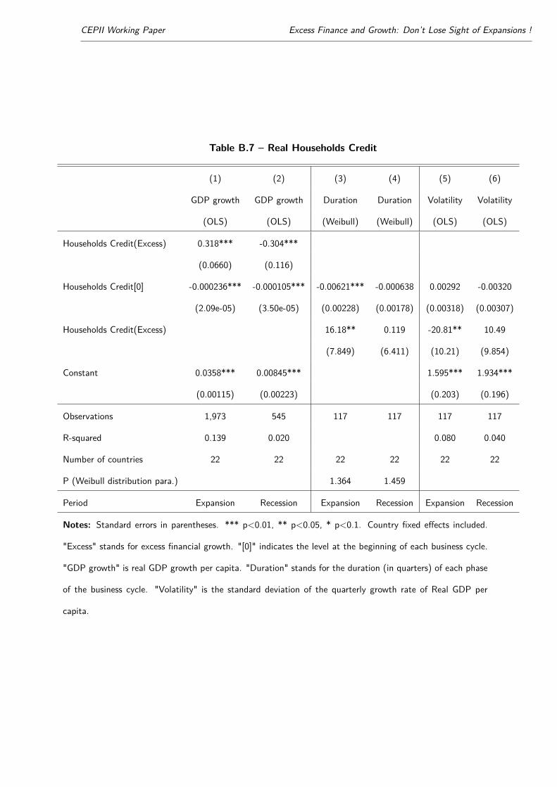
CEPII Working Paper Excess Finance and Growth: Don’t Lose Sight of Expansions !
Table B.7 – Real Households Credit
(1) (2) (3) (4) (5) (6)
GDP growth GDP growth Duration Duration Volatility Volatility
(OLS) (OLS) (Weibull) (Weibull) (OLS) (OLS)
Households Credit(Excess) 0.318*** -0.304***
(0.0660) (0.116)
Households Credit[0] -0.000236*** -0.000105*** -0.00621*** -0.000638 0.00292 -0.00320
(2.09e-05) (3.50e-05) (0.00228) (0.00178) (0.00318) (0.00307)
Households Credit(Excess) 16.18** 0.119 -20.81** 10.49
(7.849) (6.411) (10.21) (9.854)
Constant 0.0358*** 0.00845*** 1.595*** 1.934***
(0.00115) (0.00223) (0.203) (0.196)
Observations 1,973 545 117 117 117 117
R-squared 0.139 0.020 0.080 0.040
Number of countries 22 22 22 22 22 22
P (Weibull distribution para.) 1.364 1.459
Period Expansion Recession Expansion Recession Expansion Recession
Notes: Standard errors in parentheses. *** p<0.01, ** p<0.05, * p<0.1. Country fixed effects included.
"Excess" stands for excess financial growth. "[0]" indicates the level at the beginning of each business cycle.
"GDP growth" is real GDP growth per capita. "Duration" stands for the duration (in quarters) of each phase
of the business cycle. "Volatility" is the standard deviation of the quarterly growth rate of Real GDP per
capita.

CEPII Working Paper Excess Finance and Growth: Don’t Lose Sight of Expansions !
Table B.8 – Households Credit/GDP
(1) (2) (3) (4) (5) (6)
GDP growth GDP growth Duration Duration Volatility Volatility
(OLS) (OLS) (Weibull) (Weibull) (OLS) (OLS)
Households Credit/GDP(Excess) 0.264*** -0.349***
(0.0694) (0.119)
Households Credit/GDP[0] -0.0459*** -0.0138** -0.130 0.106 0.738 -0.866
(0.00382) (0.00623) (0.316) (0.239) (0.609) (0.595)
Households Credit/GDP(Excess) 34.92*** 4.596 -23.40** 1.055
(8.361) (6.681) (10.22) (9.976)
Constant 0.0447*** 0.00894*** 1.412*** 2.127***
(0.00177) (0.00315) (0.303) (0.296)
Observations 1,973 545 117 117 117 117
R-squared 0.104 0.020 0.087 0.025
Number of countries 22 22 22 22 22 22
P (Weibull distribution para.) 1.325 1.460
Period Expansion Recession Expansion Recession Expansion Recession
Notes: Standard errors in parentheses. *** p<0.01, ** p<0.05, * p<0.1. Country fixed effects included.
"Excess" stands for excess financial growth. "[0]" indicates the level at the beginning of each business cycle.
"GDP growth" is real GDP growth per capita. "Duration" stands for the duration (in quarters) of each phase of
the business cycle. "Volatility" is the standard deviation of the quarterly growth rate of Real GDP per capita.
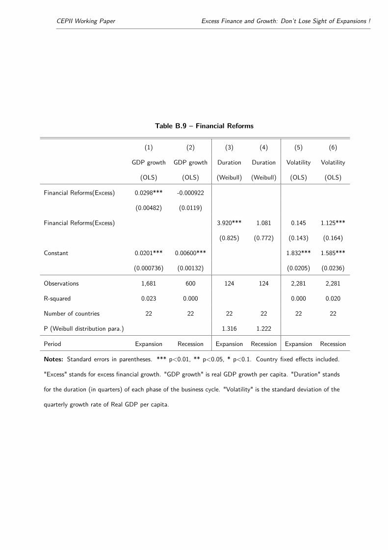
CEPII Working Paper Excess Finance and Growth: Don’t Lose Sight of Expansions !
Table B.9 – Financial Reforms
(1) (2) (3) (4) (5) (6)
GDP growth GDP growth Duration Duration Volatility Volatility
(OLS) (OLS) (Weibull) (Weibull) (OLS) (OLS)
Financial Reforms(Excess) 0.0298*** -0.000922
(0.00482) (0.0119)
Financial Reforms(Excess) 3.920*** 1.081 0.145 1.125***
(0.825) (0.772) (0.143) (0.164)
Constant 0.0201*** 0.00600*** 1.832*** 1.585***
(0.000736) (0.00132) (0.0205) (0.0236)
Observations 1,681 600 124 124 2,281 2,281
R-squared 0.023 0.000 0.000 0.020
Number of countries 22 22 22 22 22 22
P (Weibull distribution para.) 1.316 1.222
Period Expansion Recession Expansion Recession Expansion Recession
Notes: Standard errors in parentheses. *** p<0.01, ** p<0.05, * p<0.1. Country fixed effects included.
"Excess" stands for excess financial growth. "GDP growth" is real GDP growth per capita. "Duration" stands
for the duration (in quarters) of each phase of the business cycle. "Volatility" is the standard deviation of the
quarterly growth rate of Real GDP per capita.
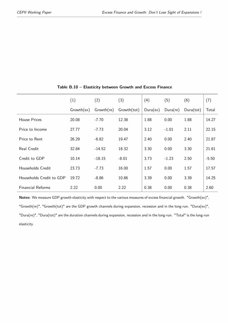
CEPII Working Paper Excess Finance and Growth: Don’t Lose Sight of Expansions !
Table B.10 – Elasticity between Growth and Excess Finance
(1) (2) (3) (4) (5) (6) (7)
Growth(ex) Growth(re) Growth(tot) Dura(ex) Dura(re) Dura(tot) Total
House Prices 20.08 -7.70 12.38 1.88 0.00 1.88 14.27
Price to Income 27.77 -7.73 20.04 3.12 -1.01 2.11 22.15
Price to Rent 26.29 -6.82 19.47 2.40 0.00 2.40 21.87
Real Credit 32.84 -14.52 18.32 3.30 0.00 3.30 21.61
Credit to GDP 10.14 -18.15 -8.01 3.73 -1.23 2.50 -5.50
Households Credit 23.73 -7.73 16.00 1.57 0.00 1.57 17.57
Households Credit to GDP 19.72 -8.86 10.86 3.39 0.00 3.39 14.25
Financial Reforms 2.22 0.00 2.22 0.38 0.00 0.38 2.60
Notes: We measure GDP growth elasticity with respect to the various measures of excess financial growth. "Growth(ex)",
"Growth(re)", "Growth(tot)" are the GDP growth channels during expansion, recession and in the long-run. "Dura(ex)",
"Dura(re)", "Dura(tot)" are the duration channels during expansion, recession and in the long-run. "Total" is the long-run
elasticity.
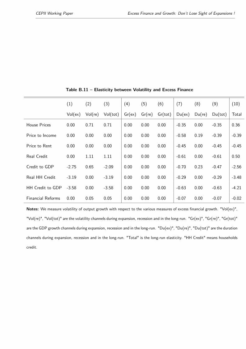
CEPII Working Paper Excess Finance and Growth: Don’t Lose Sight of Expansions !
Table B.11 – Elasticity between Volatility and Excess Finance
(1) (2) (3) (4) (5) (6) (7) (8) (9) (10)
Vol(ex) Vol(re) Vol(tot) Gr(ex) Gr(re) Gr(tot) Du(ex) Du(re) Du(tot) Total
House Prices 0.00 0.71 0.71 0.00 0.00 0.00 -0.35 0.00 -0.35 0.36
Price to Income 0.00 0.00 0.00 0.00 0.00 0.00 -0.58 0.19 -0.39 -0.39
Price to Rent 0.00 0.00 0.00 0.00 0.00 0.00 -0.45 0.00 -0.45 -0.45
Real Credit 0.00 1.11 1.11 0.00 0.00 0.00 -0.61 0.00 -0.61 0.50
Credit to GDP -2.75 0.65 -2.09 0.00 0.00 0.00 -0.70 0.23 -0.47 -2.56
Real HH Credit -3.19 0.00 -3.19 0.00 0.00 0.00 -0.29 0.00 -0.29 -3.48
HH Credit to GDP -3.58 0.00 -3.58 0.00 0.00 0.00 -0.63 0.00 -0.63 -4.21
Financial Reforms 0.00 0.05 0.05 0.00 0.00 0.00 -0.07 0.00 -0.07 -0.02
Notes: We measure volatility of output growth with respect to the various measures of excess financial growth. "Vol(ex)",
"Vol(re)", "Vol(tot)" are the volatility channels during expansion, recession and in the long-run. "Gr(ex)", "Gr(re)", "Gr(tot)"
are the GDP growth channels during expansion, recession and in the long-run. "Du(ex)", "Du(re)", "Du(tot)" are the duration
channels during expansion, recession and in the long-run. "Total" is the long-run elasticity. "HH Credit" means households
credit.
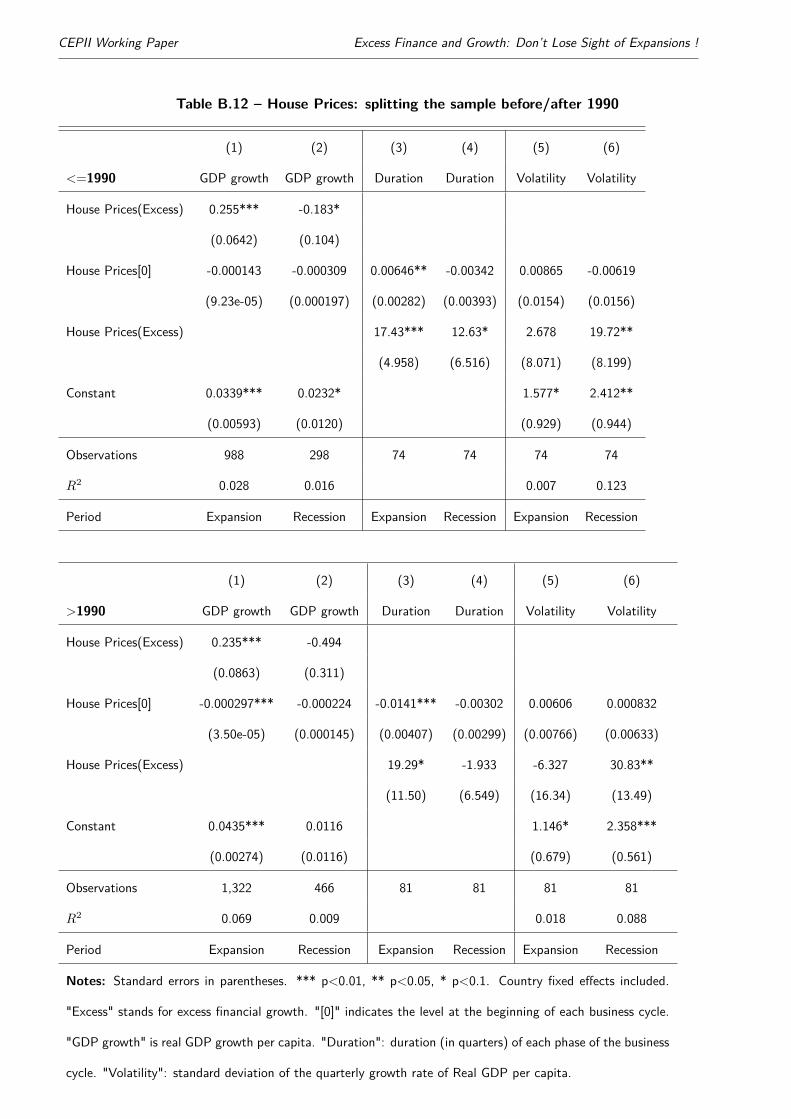
CEPII Working Paper Excess Finance and Growth: Don’t Lose Sight of Expansions !
Table B.12 – House Prices: splitting the sample before/after 1990
(1) (2) (3) (4) (5) (6)
<=1990 GDP growth GDP growth Duration Duration Volatility Volatility
House Prices(Excess) 0.255*** -0.183*
(0.0642) (0.104)
House Prices[0] -0.000143 -0.000309 0.00646** -0.00342 0.00865 -0.00619
(9.23e-05) (0.000197) (0.00282) (0.00393) (0.0154) (0.0156)
House Prices(Excess) 17.43*** 12.63* 2.678 19.72**
(4.958) (6.516) (8.071) (8.199)
Constant 0.0339*** 0.0232* 1.577* 2.412**
(0.00593) (0.0120) (0.929) (0.944)
Observations 988 298 74 74 74 74
R2 0.028 0.016 0.007 0.123
Period Expansion Recession Expansion Recession Expansion Recession
(1) (2) (3) (4) (5) (6)
>1990 GDP growth GDP growth Duration Duration Volatility Volatility
House Prices(Excess) 0.235*** -0.494
(0.0863) (0.311)
House Prices[0] -0.000297*** -0.000224 -0.0141*** -0.00302 0.00606 0.000832
(3.50e-05) (0.000145) (0.00407) (0.00299) (0.00766) (0.00633)
House Prices(Excess) 19.29* -1.933 -6.327 30.83**
(11.50) (6.549) (16.34) (13.49)
Constant 0.0435*** 0.0116 1.146* 2.358***
(0.00274) (0.0116) (0.679) (0.561)
Observations 1,322 466 81 81 81 81
R2 0.069 0.009 0.018 0.088
Period Expansion Recession Expansion Recession Expansion Recession
Notes: Standard errors in parentheses. *** p<0.01, ** p<0.05, * p<0.1. Country fixed effects included.
"Excess" stands for excess financial growth. "[0]" indicates the level at the beginning of each business cycle.
"GDP growth" is real GDP growth per capita. "Duration": duration (in quarters) of each phase of the business
cycle. "Volatility": standard deviation of the quarterly growth rate of Real GDP per capita.

CEPII Working Paper Excess Finance and Growth: Don’t Lose Sight of Expansions !
TableB.13–Variables
defin
ition
s
Variables
(Abbreviation)
Sources
Variabledescrip
tion
Totalc
redit(
Totalc
redit)
BISLo
ngserie
son
credit
to
thepriva
teno
n-fin
ancia
lsec-
tor
Creditto
non-fin
ancia
lpriv
atesector
(Borrowing
sector:Pri-
vate
non-fin
ancia
lsectorthatisresidentinthee
cono
my,Lend
-
ingsector:Allsectors),Na
tionalc
urrency,Q
uarte
rly.
Households
Credit
(Hou
se-
holdsCredit)
BISLo
ngserie
son
credit
to
thepriva
teno
n-fin
ancia
lsec-
tor
Creditto
non-fin
ancia
lpriv
ates
ector−
Creditto
Non-fin
ancia
l
Corporations,N
ationalc
urrency,Q
uarte
rly.
Gross
domestic
prod
uct
(GDP)
OEC
D,
Quarte
rlyNa
tional
Accoun
ts
Natio
nalc
urrency,
volumeestim
ates,OEC
Dreferenceyear,
annu
allev
els,seasonally
adjusted,Q
uarte
rly.
Popu
latio
n(Pop
ulation)
OEC
D,Historica
lpop
ulation
data
andprojectio
ns
Popu
latio
n,15-64,
Person
s,thou
sand
s.
GDP
percapita
(GDP
per
capita)
OEC
DGD
P/Po
pulatio
n15-64,
Quarte
rly.
56
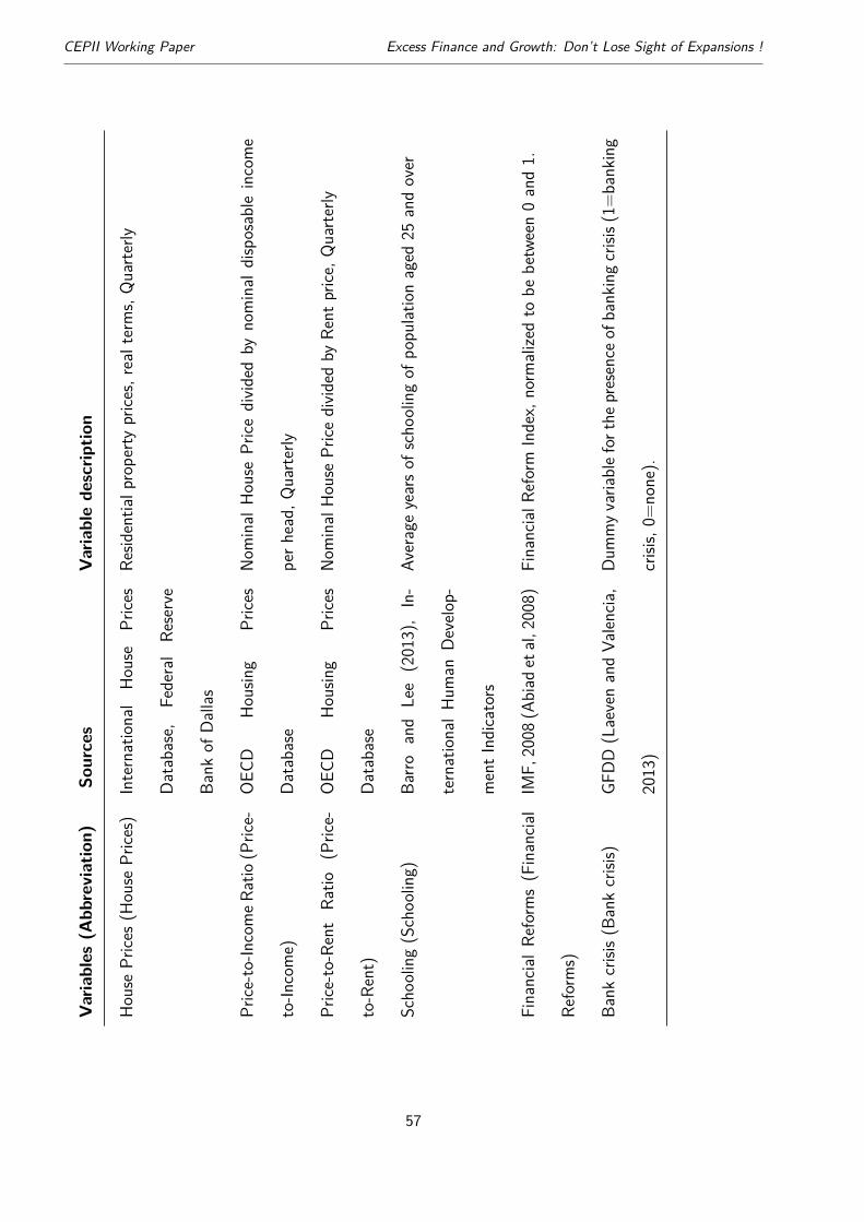
CEPII Working Paper Excess Finance and Growth: Don’t Lose Sight of Expansions !
Variables
(Abbreviation)
Sources
Variabledescrip
tion
HousePrice
s(H
ouse
Price
s)International
House
Price
s
Database,
Federal
Reserve
Bank
ofDallas
Resid
entia
lproperty
price
s,real
term
s,Quarte
rly
Price
-to-In
comeR
atio(P
rice-
to-In
come)
OEC
DHo
using
Price
s
Database
Nominal
HousePrice
divid
edby
nominal
disposable
income
perh
ead,
Quarte
rly
Price
-to-Rent
Ratio
(Pric
e-
to-Rent)
OEC
DHo
using
Price
s
Database
Nominal
HousePrice
divid
edby
Rent
price
,Quarte
rly
Scho
oling(Schoo
ling)
Barro
and
Lee
(2013),
In-
ternationalHu
man
Develo
p-
mentInd
icators
Averageyearsof
scho
olingof
popu
latio
naged
25andover
FinancialR
eforms(Financia
l
Reform
s)
IMF,
2008
(Abiad
etal,2
008)
FinancialR
eform
Index,
norm
alize
dto
bebetween0and1.
Bank
crisis(B
ankcrisis)
GFDD
(LaevenandVa
lencia
,
2013)
Dum
myvaria
blef
orthep
resenceo
fbanking
crisis(
1=banking
crisis,0=
none).
57
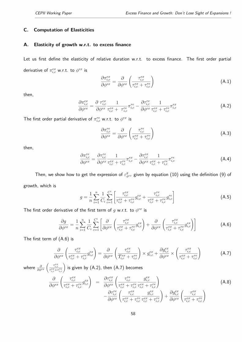
CEPII Working Paper Excess Finance and Growth: Don’t Lose Sight of Expansions !
C. Computation of Elasticities
A. Elasticity of growth w.r.t. to excess finance
Let us first define the elasticity of relative duration w.r.t. to excess finance. The first order partial
derivative of πexi,c w.r.t. to φex is∂πexi,c∂φex
= ∂
∂φex
(τ exi,c
τ exi,c + τ rei,c
)(A.1)
then,∂πexi,c∂φex
=∂ τ exi,c∂φex
1τ exi,c + τ rei,c
πrei,c −∂τ rei,c∂φex
1τ exi,c + τ rei,c
πexi,c (A.2)
The first order partial derivative of πrei,c w.r.t. to φex is
∂πrei,c∂φex
= ∂
∂φex
(τ rei,c
τ exi,c + τ rei,c
)(A.3)
then,∂πrei,c∂φex
=∂τ rei,c∂φex
1τ exi,c + τ rei,c
πexi,c −∂τ exi,c∂φex
1τ exi,c + τ rei,c
πrei,c (A.4)
Then, we show how to get the expression of εgφex given by equation (10) using the definition (9) of
growth, which is
g = 1n
n∑i=1
1Ci
Ci∑c=1
[τ exi,c
τ exi,c + τ rei,cgexi,c +
τ rei,cτ exi,c + τ rei,c
grei,c
](A.5)
The first order derivative of the first term of g w.r.t. to φex is
∂g
∂φex= 1n
n∑i=1
1Ci
Ci∑c=1
[∂
∂φex
(τ exi,c
τ exi,c + τ rei,cgexi,c
)+ ∂
∂φex
(τ exi,c
τ exi,c + τ rei,cgexi,c
)](A.6)
The first term of (A.6) is
∂
∂φex
(τ exi,c
τ exi,c + τ rei,cgexi,c
)= ∂
∂φex
(τ exi,c
T exi,c + τ rei,c
)× gexi,c +
∂gexi,c∂φex
×(
τ exi,cτ exi,c + τ rei,c
)(A.7)
where ∂∂φex
(τex
i,c
τexi,c+τre
i,c
)is given by (A.2), then (A.7) becomes
∂
∂φex
(τ exi,c
τ exi,c + τ rei,cgexi,c
)=
∂τ exi,c∂φex
(τ rei,c
τ exi,c + τ rei,c
gexi,cτ exi,c + τ rei,c
)(A.8)
−∂τ rei,c∂φex
(τ exi,c
τ exi,c + τ rei,c
gexi,cτ exi,c + τ rei,c
)+∂gexi,c∂φex
(τ exi,c
τ exi,c + τ rei,c
)
58
CEPII Working Paper Excess Finance and Growth: Don’t Lose Sight of Expansions !
The second term of (A.6) is
∂
∂φex
(τ rei,c
τ exi,c + τ rei,cgrei,c
)= ∂
∂φex
(τ rei,c
T exi,c + τ rei,c
)× grei,c +
(τ exi,c
τ exi,c + τ rei,c
)×∂grei,c∂φex
(A.9)
where ∂∂φex
(τre
i,c
τexi,c+τre
i,c
)is given by (A.4), then (A.9) becomes
∂
∂φex
(τ rei,c
τ exi,c + τ rei,cgrei,c
)=
∂τ rei,c∂φex
(τ exi,c
τ exi,c + τ rei,c
grei,cτ exi,c + τ rei,c
)(A.10)
−∂τ exi,c∂φex
(τ rei,c
τ exi,c + τ rei,c
grei,cτ exi,c + τ rei,c
)+∂grei,c∂φex
(τ exi,c
τ exi,c + τ rei,c
)
The sum of (A.8) and (A.10) is
∂
∂φex
(τ exi,c
τ exi,c + τ rei,cgexi,c
)+ ∂
∂φex
(τ exi,c
T exi,c + τ rei,cgexi,c
)(A.11)
=∂gexi,c∂φex
(τ exi,c
τ exi,c + τ rei,c
)+∂grei,c∂φex
(τ exi,c
τ exi,c + τ rei,c
)+(∂τ exi,c∂φex
τ rei,c −∂τ rei,c∂φex
τ exi,c
)gexi,c − grei,c(τ exi,c + τ rei,c
)2
that is the term in the sum defined by equation (10). Using (13) and (15), (A.11) becomes
∂
∂φex
(τ exi,c
τ exi,c + τ rei,cgexi,c
)+ ∂
∂φex
(τ exi,c
T exi,c + τ rei,cgexi,c
)(A.12)
= αexg
(τ exi,c
τ exi,c + τ rei,c
)+ αreg
(τ exi,c
τ exi,c + τ rei,c
)+ (αexτ − αreτ )
τ exi,c τrei,c(
τ exi,c + τ rei,c)2
(gexi,c − grei,c
)
Introducing this expression into (A.6) gives
∂g
∂φex= αexg ×
1n
n∑i=1
1Ci
Ci∑c=1
(τ exi,c
τ exi,c + τ rei,c
)+ αreg ×
1n
n∑i=1
1Ci
Ci∑c=1
[(τ rei,c
τ exi,c + T rei,c
)](A.13)
+ (αexτ − αreτ )× 1n
n∑i=1
1Ci
Ci∑c=1
τ exi,c τrei,c(
τ exi,c + τ rei,c)2
(gexi,c − grei,c
)using the definition of πphi,c = τ phi,c /
(τ exi,c + τ rei,c
)and σi,c = πexi,cπ
rei,c
(gexi,c − grei,c
), it becomes
∂g
∂φex= αexg ×
1n
n∑i=1
1Ci
Ci∑c=1
πexi,c + αreg ×1n
n∑i=1
1Ci
Ci∑c=1
πrei,c (A.14)
+ (αexτ − αreτ )× 1n
n∑i=1
1Ci
Ci∑c=1
σi,c
and, finally, using the x̃ symbol to denote historical mean of series x, it is
∂g
∂φex= αexg × π̃ex + αreg × π̃re + (αexT − αreτ )× σ̃ (A.15)
59
CEPII Working Paper Excess Finance and Growth: Don’t Lose Sight of Expansions !
B. Definition of the Variance of Growth
The variance of growth during the cycle c in country i is defined as follows
var (gi,c) ≡1τi,c
τi,c∑s=1
(gi,c,s − g̃i,c)2 (B.1)
Using the definition of business cycle phases, it is
var (gi,c) = 1τi,c
τexi,c∑s=1
(gi,c,s − g̃i,c)2 +τi,c∑
s=1+τexi,c
(gi,c,s − g̃i,c)2
(B.2)
Introducing the average values of growth rate per business cycle phases ph, namely gphi,c for ph = {ex, re},
it becomes
var (gi,c) = 1τi,c
τexi,c∑s=1
[(gi,c,∫ − gexi,c
)+(gexi,c − g̃i,c
)]2+
τi,c∑s=1+τex
i,c
[(gi,c,s − grei,c
)+(grei,c − g̃i,c
)]2 (B.3)
The first term of (B.3) is
τexi,c∑s=1
[(gi,c,s − gexi,c
)+(gexi,c − g̃i,c
)]2=
τexi,c∑s=1
[(gi,c,s − gexi,c
)2+(gexi,c − g̃i,c
)2+ 2
(gi,c,s − gexi,c
) (gexi,c − g̃i,c
)](B.4)
then,
τexi,c∑s=1
[(gi,c,s − gexi,c
)+(gexi,c − g̃i,c
)]2(B.5)
= τ exi,c
1τ exi,c
τexi,c∑s=1
(gi,c,s − gexi,c
)2
︸ ︷︷ ︸=var(gex
i,c)
+2(gexi,c − g̃i,c
) 1τ exi,c
τexi,c∑s=1
gi,c,s︸ ︷︷ ︸=gex
i,c
+(gexi,c − g̃i,c
)2− 2gexi,c
(gexi,c − g̃i,c
)
and finallyτex
i,c∑s=1
[(gi,c,s − gexi,c
)+(gexi,c − g̃i,c
)]2= τ exi,cvar
(gexi,c)
+ τ exi,c(gexi,c − g̃i,c
)2(B.6)
The second term of (B.3) is
τi,c∑s=1+τex
i,c
[(gi,c,s − grei,c
)+(grei,c − g̃i,c
)]2= τ rei,cvar
(grei,c)
+ τ rei,c(grei,c − g̃i,c
)2(B.7)
60

CEPII Working Paper Excess Finance and Growth: Don’t Lose Sight of Expansions !
following similar calculus. Using (B.6) and (B.7), (B.3) becomes
var (gi,c) = 1τi,c
[τ exi,cvar
(gexi,c)
+ τ exi,c(gexi,c − g̃i,c
)2+ τ rei,cvar
(grei,c)
+ τ rei,c(grei,c − g̃i,c
)2]
(B.8)
Then, introducing the variables πph, it becomes
var (gi,c) = πexi,cvar(gexi,c)
+ πrei,cvar(grei,c)
+ πexi,c(gexi,c − g̃i,c
)2+ πrei,c
(grei,c − g̃i,c
)2(B.9)
The last step is to suppress g̃i,c form this expression, using
g̃i,c ≡ πexi,cgexi,c + πrei,cg
rei,c (B.10)
then
var (gi,c) = πexi,cvar(gexi,c)
+πrei,cvar(grei,c)
+πexi,c((
1− πexi,c)gexi,c − πrei,cgrei,c
)2+πrei,c
((1− πrei,c
)grei,c − πexi,cgexi,c
)2
(B.11)
since πrei,c + πexi,c = 1, it becomes
var (gi,c) = πexi,cvar(gexi,c)
+ πrei,cvar(grei,c)
+ πexi,c(πrei,c
)2 (gexi,c − grei,c
)2+ πrei,c
(πexi,c
)2 (grei,c − gexi,c
)2(B.12)
and finally,
var (gi,c) = πexi,cvar(gexi,c)
+ πrei,cvar(grei,c)
+ πexi,cπrei,c
(gexi,c − grei,c
)2(B.13)
C. Elasticity of the Variance of Growth w.r.t. Excess Finance
The first order partial derivative of var (gi,c) w.r.t. to φex is
∂var (gi,c)∂φex
=∂πexi,c∂φex
var(gexi,c)
+ πexi,c∂var
(gexi,c)
∂φex+∂πrei,c∂φex
var(grei,c)
+ πrei,c∂var
(grei,c)
∂φex(C.1)
+
∂(πexi,cπ
rei,c
)∂φex
(gexi,c − grei,c
)2+ πexi,cπ
rei,c
∂(gexi,c − grei,c
)2
∂φex
The first order partial derivative of var
(gphi,c)w.r.t. to φex is
∂var(gphi,c)
∂φex= 2
dsd(gphi,c)
∂φexsd(gphi,c)
(C.2)
61
CEPII Working Paper Excess Finance and Growth: Don’t Lose Sight of Expansions !
using the definition of the variance: var(gphi,c)≡ sd
(gphi,c)2. The first order partial derivative of πexi,c w.r.t.
to φex is given by (A.2), which becomes
∂πexi,c∂φex
= 1τ exi,c + τ rei,c
(αexτ
τ exi,c τrei,c
τ exi,c + τ rei,c− αreτ
τ rei,cτexi,c
τ exi,c + τ rei,c
)(C.3)
using (15), and then,∂πexi,c∂φex
= πexi,cπrei,c (αexτ − αreτ ) (C.4)
The first order partial derivative of πrei,c w.r.t. to φex is is given by (A.4), which becomes
∂πrei,c∂φex
= 1τ exi,c + τ rei,c
(αreτ
τ rei,cτexi,c
τ exi,c + τ rei,c− αexτ
τ exi,c τrei,c
τ exi,c + τ rei,c
)(C.5)
using (15), and then,∂πrei,c∂φex
= πexi,cπrei,c (αreτ − αexτ ) (C.6)
or equivalently,∂πrei,c∂φex
= −πexi,cπrei,c (αexτ − αreτ ) = −∂πexi,c∂φex
(C.7)
The first order partial derivative of(πexi,cπ
rei,c
)w.r.t. to φex is
∂(πexi,cπ
rei,c
)∂φex
=∂πexi,c∂φex
πrei,c +∂πrei,c∂φex
πexi,c (C.8)
using (C.7) and πrei,c = 1− πexi,c, it becomes
∂(πexi,cπ
rei,c
)∂φex
=∂πexi,c∂φex
(1− 2πexi,c
)(C.9)
and using (C.4)∂(πexi,cπ
rei,c
)∂φex
= πexi,cπrei,c
(1− 2πexi,c
)(αexτ − αreτ ) (C.10)
The first order partial derivative of(gexi,c − grei,c
)2w.r.t. to φex is
∂(gexi,c − grei,c
)2
∂φex= 2
(∂gexi,c∂φex
−∂grei,c∂φex
)(gexi,c − grei,c
)(C.11)
62
CEPII Working Paper Excess Finance and Growth: Don’t Lose Sight of Expansions !
Using (13), it becomes∂(gexi,c − grei,c
)2
∂φex= 2
(αexg − αreg
) (gexi,c − grei,c
)(C.12)
Finally, (C.1) becomes
∂var (gi,c)∂φex
= πexi,c × 2dsd
(gexi,c)
∂φexsd(gexi,c)
+ πrei,c × 2dsd
(grei,c)
∂φexsd(grei,c)
(C.13)
+πexi,cπrei,cvar(gexi,c)
(αexτ − αreτ )− πexi,cπrei,cvar(grei,c)
(αexτ − αreτ )
+(gexi,c − grei,c
)2πexi,cπ
rei,c
(1− 2πexi,c
)(αexτ − αreτ ) + πexi,cπ
rei,c2
(gexi,c − grei,c
) (αexg − αreg
)
using (C.4), (C.6), and (C.12), and then
∂var (gi,c)∂φex
= πexi,c × 2dsd
(gexi,c)
∂φexsd(gexi,c)
+ πrei,c × 2dsd
(grei,c)
∂φexsd(grei,c)
(C.14)
+πexi,cπrei,c[var
(gexi,c)− var
(grei,c)
+(gexi,c − grei,c
)2 (1− 2πexi,c
)](αexτ − αreτ )
+ + πexi,cπrei,c2
(gexi,c − grei,c
) (αexg − αreg
)
Using (22), it becomes
∂var (gi,c)∂φex
= πexi,c × 2αexsdsd(gexi,c)
+ πrei,c × 2αresdsd(grei,c)
+ πexi,cπrei,c2
(gexi,c − grei,c
) (αexg − αreg
)(C.15)
+πexi,cπrei,c[var
(gexi,c)− var
(grei,c)
+(gexi,c − grei,c
)2 (1− 2πexi,c
)](αexτ − αreτ )
The last step is to take the historical average of this first order partial derivative to get equation 22
assuming here that the covariance cov (gi,c, gi,c′) is not related to φex consistently with the next Section
D.
D. Definition of the Covariance of Growth
Using the definitions (4) and (5), growth during the cycle c in country i is
gi,c ≡1
τ exi,c + τ rei,c
τexi,c∑s=1
gexi,c,s +τi,c∑
s=τexi,c+1
grei,c,s
(D.1)
The covariance between gi,c and gi,c′ is defined as
cov (gi,c, gi,c′) ≡ E [(gi,c − E (gi,c)) (gi,c′ − E (gi,c′))] (D.2)
63
CEPII Working Paper Excess Finance and Growth: Don’t Lose Sight of Expansions !
where the expected value for growth is
E (gi,c) = E 1τ exi,c + τ rei,c
τ exi,c (cexg + F exg,i + αexg φ
ex)
+τex
i,c∑∫=1
γphg Xgi,c,s +
τexi,c∑s=1
εi,c,s
+ τ rei,c(creg + F re
g,i + αreg φex)
+τi,c∑
s=τexi,c+1
γreg Xgi,c,s +
τi,c∑∫=τex
i,c+1εi,c,s
using the regressions (12). Then, the gap between gi,c and its expected value is the weigthed sum of
shocks
gi,c − E (gi,c) = 1τ exi,c + τ rei,c
τexi,c∑s=1
εi,c,s +τi,c∑
s=τexi,c+1
εi,c,∫
(D.3)
The covariance defined by (D.2) is then
cov (gi,c, gi,c′) = E
1τ exi,c + τ rei,c
τexi,c∑∫=1
εi,c,s + 1τ exi,c + τ rei,c
τi,c∑s=τex
i,c+1εi,c,∫
×
1τ exi,c′ + τ rei,c′
τexi,c′∑s=1
εi,c′,s + 1τ exi,c′ + τ rei,c′
τi,c′∑s=τex
i,c′ +1εi,c′,s
and
cov (gi,c, gi,c′) (D.4)
= E
1τ exi,c + τ rei,c
1τ exi,c′ + τ rei,c′
τexi,c∑s=1
εi,c,s
τexi,c′∑∫=1
εi,c′,s + 1τ exi,c + τ rei,c
1τ exi,c′ + τ rei,c′
τexi,c∑s=1
εi,c,∫
τi,c′∑s=τex
i,c′ +1εi,c′,s
+
1τ exi,c + τ rei,c
1τ exi,c′ + τ rei,c′
τi,c∑s=τex
i,c+1εi,c,s
T exi,c′∑s=1
εi,c′,s + 1τ exi,c′ + τ rei,c′
1τ exi,c + τ rei,c
τi,c∑s=T ex
i,c +1εi,c,s
τi,c′∑s=τex
i,c′ +1εi,c′,s
Since residuals εi,c,s are assumed to be iid with a zero mean, they satisfy E (εi,c,∫ ) = E (εi,c′,s) = 0 with
cov (εi,c,s, εi,c′,s) = 0, which imply cov (gi,c, gi,c′) = 0 in (D.2).
64