Embed Size (px)
Citation preview

March, 2002 EditionCopyright © Research Systems, Inc.All Rights Reserved
Excerpts From:
Working withImages in IDL
Restricted Rights NoticeThe IDL® software program and the accompanying procedures, functions, and documenta-tion described herein are sold under license agreement. Their use, duplication, and disclo-sure are subject to the restrictions stated in the license agreement. Research Systems, Inc.,reserves the right to make changes to this document at any time and without notice.
Limitation of WarrantyResearch Systems, Inc. makes no warranties, either express or implied, as to any matter notexpressly set forth in the license agreement, including without limitation the condition ofthe software, merchantability, or fitness for any particular purpose.
Research Systems, Inc. shall not be liable for any direct, consequential, or other damagessuffered by the Licensee or any others resulting from use of the IDL software package or itsdocumentation.
Permission to Reproduce this ManualIf you are a licensed user of this product, Research Systems, Inc. grants you a limited, non-transferable license to reproduce this particular document provided such copies are for youruse only and are not sold or distributed to third parties. All such copies must contain the titlepage and this notice page in their entirety.
AcknowledgmentsIDL® is a registered trademark of Research Systems Inc., registered in the United States Patent and Trademark Office, forthe computer program described herein. Software ≡ Vision™ is a trademark of Research Systems, Inc.
Numerical Recipes™ is a trademark of Numerical Recipes Software. Numerical Recipes routines are used by permission.
GRG2™ is a trademark of Windward Technologies, Inc. The GRG2 software for nonlinear optimization is used by permis-sion.
NCSA Hierarchical Data Format (HDF) Software Library and UtilitiesCopyright © 1988-1998 The Board of Trustees of the University of IllinoisAll rights reserved.
CDF LibraryCopyright © 1999National Space Science Data CenterNASA/Goddard Space Flight Center
NetCDF LibraryCopyright © 1993-1996 University Corporation for Atmospheric Research/Unidata
HDF EOS LibraryCopyright © 1996 Hughes and Applied Research Corporation
This software is based in part on the work of the Independent JPEG Group.
This product contains StoneTable™, by StoneTablet Publishing. All rights to StoneTable™ and its documentation areretained by StoneTablet Publishing, PO Box 12665, Portland OR 97212-0665. Copyright © 1992-1997 StoneTablet Publish-ing
WASTE text engine © 1993-1996 Marco Piovanelli
Portions of this software are copyrighted by INTERSOLV, Inc., 1991-1998.
Other trademarks and registered trademarks are the property of the respective trademark holders.
imgdispl.fm Page 1 Wednesday, March 6, 2002 5:29 PM
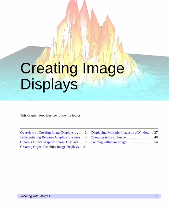
Creating ImageDisplays
This chapter describes the following topics:
Overview of Creating Image Displays . . . . . 2Differentiating Between Graphics Systems . 4
Creating Direct Graphics Image Displays . . 7Creating Object Graphics Image Displays . 21
Displaying Multiple Images in a Window . . 37Zooming in on an Image . . . . . . . . . . . . . . . 48
Panning within an Image . . . . . . . . . . . . . . . 54
Working with Images 1
2 Creating Image Displays
imgdispl.fm Page 2 Wednesday, March 6, 2002 5:29 PM
Overview of Creating Image Displays
To understand how to display an image, you must understand IDL’s graphics systems,window coordinate systems, and the types of images you can display. IDL has twotypes of graphics systems, Direct and Object. Direct Graphics displays directly to awindow. Object Graphics uses object-oriented programming to display withininstances of window objects. For more information, see “Differentiating BetweenGraphics Systems” on page 4
One of IDL’s three window coordinate systems controls the placement of the imagewithin Direct and Object Graphics displays. These window coordinate systems aredata, device, and normalized. Data coordinates are the same as device coordinates forimages. Device coordinates are based on the pixel locations of an image. Normalizedcoordinates range from zero and one and are based on the width and height of theimage. See “Understanding Windows and Related Device Coordinates” on page 5 formore information.
IDL can display four types of images; binary, grayscale, indexed, and RGB. IDLtreats binary and grayscale images as a subsets of indexed images. How the image isdisplayed depends on its type. Binary images have only two values, 0 and 1.Grayscale images represent intensities and use a normal grayscale color table.Indexed images use an associated color table. RGB images contain their own colorinformation in layers known as bands or channels.Any of these images can bedisplayed with Direct Graphics, see “Creating Direct Graphics Image Displays” onpage 7, or Object Graphics, see “Creating Object Graphics Image Displays” onpage 21.
Multiple images can also be displayed in the same. The location of the imagesdepends on the window coordinate system. For more information, see “DisplayingMultiple Images in a Window” on page 37.
You can magnify specific areas of an image by changing the display show just thatregion. This magnification is known as zooming in on the image. By zooming in onan area, you can visualize each pixel that make up a feature or a boundary. See“Zooming in on an Image” on page 48 for more information.
When you zoom in on a feature within an image, you may want to move along thefeature at that magnification. The movement is known as panning. For moreinformation on panning, see “Panning within an Image” on page 54.
Overview of Creating Image Displays Working with Images
Creating Image Displays 3
imgdispl.fm Page 3 Wednesday, March 6, 2002 5:29 PM
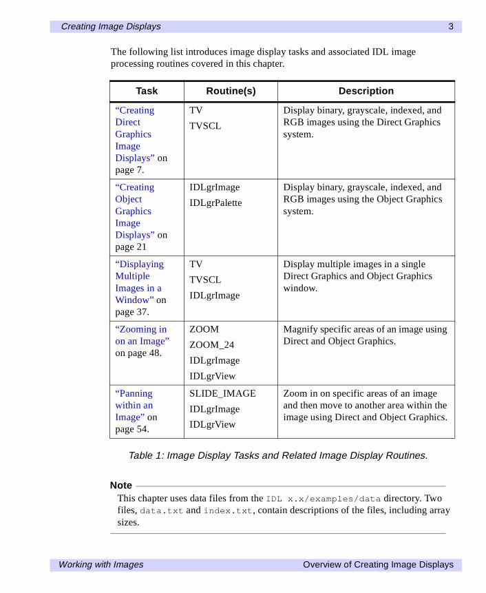
The following list introduces image display tasks and associated IDL imageprocessing routines covered in this chapter.
NoteThis chapter uses data files from the IDL x.x/examples/data directory. Twofiles, data.txt and index.txt, contain descriptions of the files, including arraysizes.
Task Routine(s) Description
“CreatingDirectGraphicsImageDisplays” onpage 7.
TV
TVSCL
Display binary, grayscale, indexed, andRGB images using the Direct Graphicssystem.
“CreatingObjectGraphicsImageDisplays” onpage 21
IDLgrImage
IDLgrPalette
Display binary, grayscale, indexed, andRGB images using the Object Graphicssystem.
“DisplayingMultipleImages in aWindow” onpage 37.
TV
TVSCL
IDLgrImage
Display multiple images in a singleDirect Graphics and Object Graphicswindow.
“Zooming inon an Image”on page 48.
ZOOM
ZOOM_24
IDLgrImage
IDLgrView
Magnify specific areas of an image usingDirect and Object Graphics.
“Panningwithin anImage” onpage 54.
SLIDE_IMAGE
IDLgrImage
IDLgrView
Zoom in on specific areas of an imageand then move to another area within theimage using Direct and Object Graphics.
Table 1: Image Display Tasks and Related Image Display Routines.
Working with Images Overview of Creating Image Displays
4 Creating Image Displays
imgdispl.fm Page 4 Wednesday, March 6, 2002 5:29 PM
Differentiating Between Graphics Systems
IDL supports two distinct graphics modes: Direct Graphics and Object Graphics.Direct Graphics rely on the concept of a current graphics device; IDL commands likeTV or PLOT create displays directly on the current graphics device. Object Graphicsuse an object-oriented programmer’ interface to create graphic objects, which mustthen be drawn, explicitly, to a destination of the programmer’s choosing.
Direct Graphics
The important aspects of Direct Graphics are:
• Direct Graphics use a graphics device (X for X-windows systems displays,WIN for Microsoft Windows displays, MAC for Macintosh displays, PS forPostScript files, etc.). You switch between graphics devices using theSET_PLOT command, and control the features of the current graphics deviceusing the DEVICE command.
• Commands like TV, PLOT, XYOUTS, MAP_SET, etc. all draw their outputdirectly on the current graphics device.
• Once a direct-mode graphic is drawn to the graphics device, it cannot bealtered or re-used. This means that if you wish to recreate the graphic on adifferent device, you must reissue the IDL commands to create the graphic.
• When you add a new item to an existing direct-mode graphic (using a routinelike OPLOT or XYOUTS), the new item is drawn in front of the existingitems.
Object Graphics
The important aspects of Object Graphics are:
• Object graphics are device independent. There is no concept of a currentgraphics device when using object-mode graphics; any graphics object can bedisplayed on any physical device for which a destination object can be created.
• Object graphics are object-oriented. Graphic objects are meant to be createdand reused; you may create a set of graphic objects, modify their attributes,draw them to a window on your computer screen, modify their attributes again,then draw them to a printer device without reissuing all of the IDL commandsused to create the objects. Graphics objects also encapsulate functionality; thismeans that individual objects include method routines that providefunctionality specific to the individual object.
Differentiating Between Graphics Systems Working with Images
Creating Image Displays 5
imgdispl.fm Page 5 Wednesday, March 6, 2002 5:29 PM
• Object graphics are rendered in three dimensions. Rendering implies manyoperations not needed when drawing Direct Graphics, including calculation ofnormal vectors for lines and surfaces, lighting considerations, and generalobject overhead. As a result, the time needed to render a given object—asurface, say—will often be longer than the time taken to draw the analogousimage in Direct Graphics.
• Object Graphics use a programmer’s interface. Unlike Direct Graphics, whichare well suited for both programming and interactive, ad hoc use, ObjectGraphics are designed to be used in programs that are compiled and run. Whileit is still possible to create and use graphics objects directly from the IDLcommand line, the syntax and naming conventions make it more convenient tobuild a program offline than to create graphics objects on the fly.
• Because Object Graphics persist in memory, there is a greater need for theprogrammer to be cognizant of memory issues and memory leakage. Efficientdesign—remembering to destroy unused object references and cleaning up—will avert most problems, but even the best designs can be memory-intensive iflarge numbers of graphic objects (or large datasets) are involved.
Understanding Windows and Related Device Coordinates
Images are displayed within a window (Direct Graphics) or within an instance of awindow object (Object Graphics). In Direct Graphics, the WINDOW procedure isused to initialize the coordinates system for the image display. In Object Graphics,the IDLgrWindow, IDLgrView, and IDLgrModel objects are used to initialize thecoordinate system for the image display.
A coordinate system determines how and where the image appears within thewindow. You can specify coordinates to IDL using one of the following coordinatesystems:
• Data Coordinates - This system usually spans the window with a rangeidentical to the range of the data. The system can have two or three dimensionsand can be linear, logarithmic, or semi-logarithmic.
• Device Coordinates - This coordinate system is the physical coordinate systemof the selected device. Device coordinates are integers, ranging from (0, 0) atthe bottom-left corner to (Vx –1, Vy –1) at the upper-right corner of the display.Vx and Vy are the number of columns and rows of the device (a display windowfor example).
Working with Images Differentiating Between Graphics Systems
6 Creating Image Displays
imgdispl.fm Page 6 Wednesday, March 6, 2002 5:29 PM
NoteFor images, the data coordinates are the same as the device coordinates. Thedevices coordinates of an image are directly related to the pixel (data) locationswithin an image.
• Normal Coordinates - The normalized coordinate system ranges from zero toone over columns and rows of the device.
Differentiating Between Graphics Systems Working with Images
Creating Image Displays 7
imgdispl.fm Page 7 Wednesday, March 6, 2002 5:29 PM
Creating Direct Graphics Image Displays
The procedure used to display an image in Direct Graphics depends upon the type ofimage to be displayed. Binary, grayscale, and indexed images are two-dimensionalarrays. In Direct Graphics, these images are displayed with the TV or TVSCLprocedures. The TV procedure displays the image in its original form. The TVSCLprocedure displays the image scaled to range from 0 up to 255 depending on thecolors available to IDL. Three dimensional RGB images are displayed with the TVprocedure.
Examples of creating such displays are shown in the following sections:
• “Displaying Binary Images with Direct Graphics”.
• “Displaying Grayscale Images with Direct Graphics” on page 10.
• “Displaying Indexed Images with Direct Graphics” on page 12.
• “Displaying RGB Images with Direct Graphics” on page 16.
Displaying Binary Images with Direct Graphics
Binary images are composed of pixels having one of two values, usually zero or one.With most color tables, pixels having values of zero or one are displayed with almostthe same color, especially with a normal grayscale color table. Thus, a binary imageis usually shown in a scaled display to show the zeros as black and the ones as white.
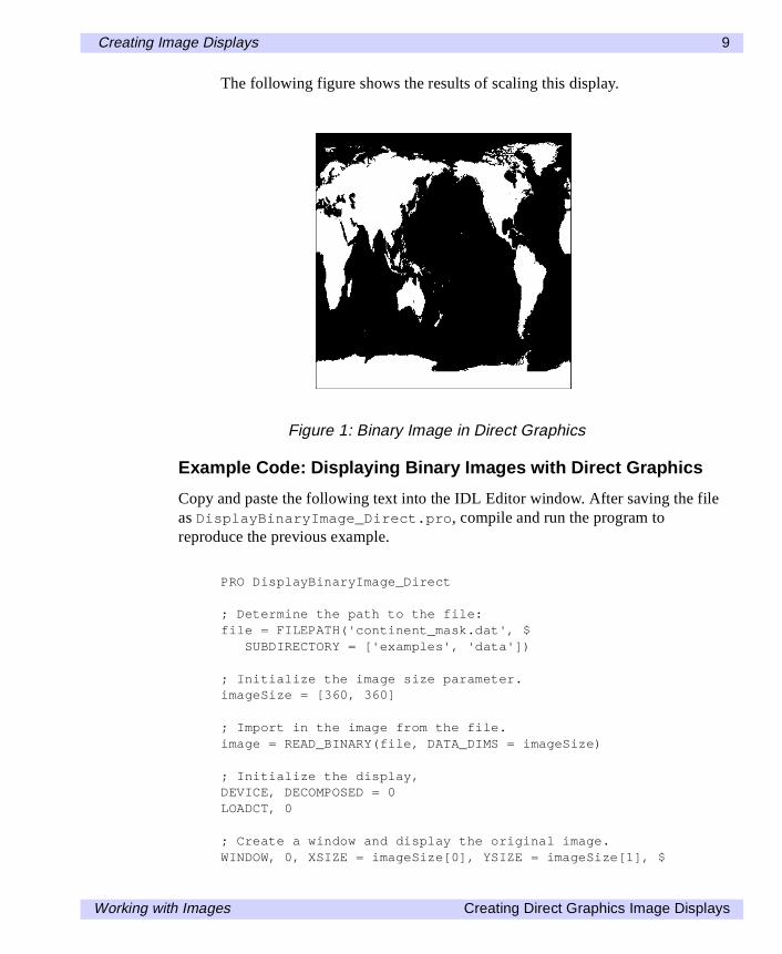
The following example imports a binary image of the world from thecontinent_mask.dat binary file. In this image, the oceans are zeros (black) andthe continents are ones (white). This type of image can be used to mask out (omit)data over the oceans. The image contains byte data values and is 360 pixels by 360pixels.
For code that you can copy and paste into an Editor window, see “Example Code:Displaying Binary Images with Direct Graphics” on page 9 or complete the followingsteps for a detailed description of the process.
1. Determine the path to the continent_mask.dat file:
file = FILEPATH('continent_mask.dat', $SUBDIRECTORY = ['examples', 'data'])
2. Initialize the image size parameter:
imageSize = [360, 360]
Working with Images Creating Direct Graphics Image Displays
8 Creating Image Displays
imgdispl.fm Page 8 Wednesday, March 6, 2002 5:29 PM
3. Use READ_BINARY to import the image from the file:
image = READ_BINARY(file, DATA_DIMS = imageSize)
4. If you are running IDL on a TrueColor display, set the DECOMPOSEDkeyword to the DEVICE command to zero before your first color table relatedroutine is used within an IDL session or program. See “How Colors areAssociated with Indexed and RGB Images” on page 84 for more information.
DEVICE, DECOMPOSED = 0
5. Load a grayscale color table:
LOADCT, 0
6. Create a window and display the original image with the TV procedure:
WINDOW, 0, XSIZE = imageSize[0], YSIZE = imageSize[1], $TITLE = 'A Binary Image, Not Scaled'
TV, image
The resulting window should be all black (blank). The binary image containszeros and ones, which are almost the same color (black). Binary images shouldbe displayed with the TVSCL procedure in order to scale the ones to white.
7. Create another window and display the scaled binary image:
WINDOW, 1, XSIZE = imageSize[0], YSIZE = imageSize[1], $TITLE = 'A Binary Image, Scaled'
TVSCL, image
Creating Direct Graphics Image Displays Working with Images
Creating Image Displays 9
imgdispl.fm Page 9 Wednesday, March 6, 2002 5:29 PM
The following figure shows the results of scaling this display.
Example Code: Displaying Binary Images with Direct Graphics
Copy and paste the following text into the IDL Editor window. After saving the fileas DisplayBinaryImage_Direct.pro, compile and run the program toreproduce the previous example.
PRO DisplayBinaryImage_Direct
; Determine the path to the file:file = FILEPATH('continent_mask.dat', $
SUBDIRECTORY = ['examples', 'data'])
; Initialize the image size parameter.imageSize = [360, 360]
; Import in the image from the file.image = READ_BINARY(file, DATA_DIMS = imageSize)
; Initialize the display,DEVICE, DECOMPOSED = 0LOADCT, 0
; Create a window and display the original image.WINDOW, 0, XSIZE = imageSize[0], YSIZE = imageSize[1], $
Figure 1: Binary Image in Direct Graphics
Working with Images Creating Direct Graphics Image Displays
10 Creating Image Displays
imgdispl.fm Page 10 Wednesday, March 6, 2002 5:29 PM
TITLE = 'A Binary Image, Not Scaled'TV, image
; Create another window and display the image scaled; to range from 0 up to 255.WINDOW, 1, XSIZE = imageSize[0], YSIZE = imageSize[1], $
TITLE = 'A Binary Image, Scaled'TVSCL, image
END
Displaying Grayscale Images with Direct Graphics
Features within grayscale images are created by pixels that have varying intensities.Pixel values range from least intense (black) to the most instance (white). Since agrayscale image is composed of pixels of varying intensities, it is best displayed witha color table that progresses linearly from black to white. Although IDL has severalsuch predefined color tables, the grayscale color table (B-W LINEAR), is the mostfitting choice when displaying grayscale images.
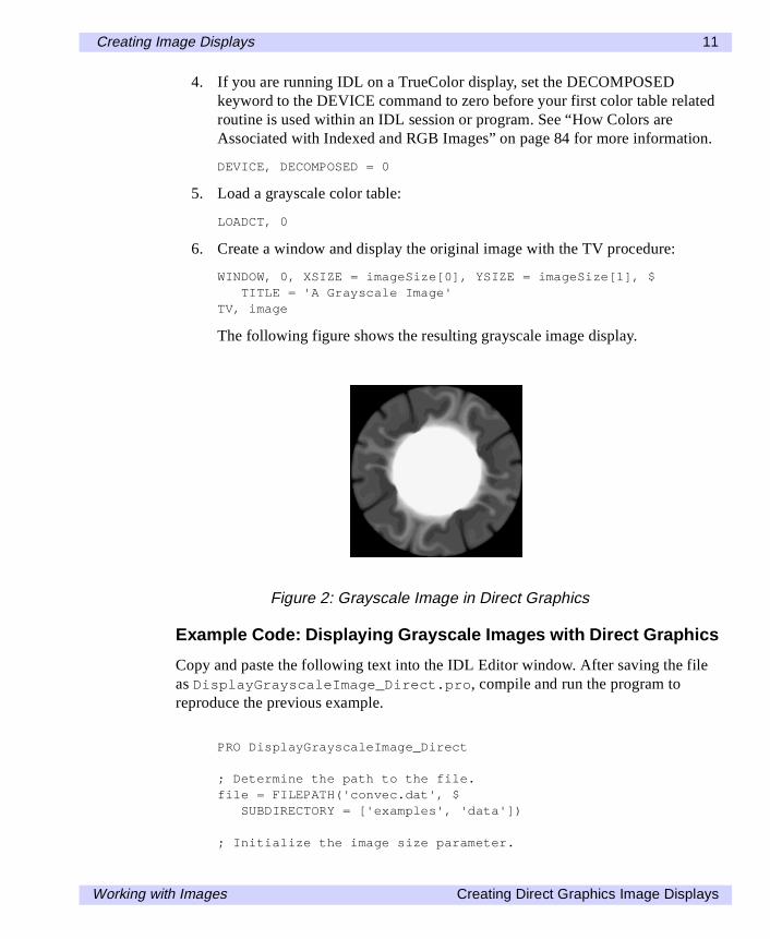
The following example imports a grayscale image from the convec.dat binary file.This grayscale image shows the convection of the Earth’s mantle. The image containsbyte data values and is 248 pixels by 248 pixels. Since the data type is byte, thisimage does not need to by scaled before display. If the data was of any type other thanbyte and the data values were not within the range of 0 up to 255, the display wouldneed to scale the image in order to show its intensities.
For code that you can copy and paste into an Editor window, see “Example Code:Displaying Grayscale Images with Direct Graphics” on page 11 or complete thefollowing steps for a detailed description of the process.
1. Determine the path to the convec.dat file:
file = FILEPATH('convec.dat', $SUBDIRECTORY = ['examples', 'data'])
2. Initialize the image size parameter:
imageSize = [248, 248]
3. Using READ_BINARY, import the image from the file:
image = READ_BINARY(file, DATA_DIMS = imageSize)
Creating Direct Graphics Image Displays Working with Images
Creating Image Displays 11
imgdispl.fm Page 11 Wednesday, March 6, 2002 5:29 PM
4. If you are running IDL on a TrueColor display, set the DECOMPOSEDkeyword to the DEVICE command to zero before your first color table relatedroutine is used within an IDL session or program. See “How Colors areAssociated with Indexed and RGB Images” on page 84 for more information.
DEVICE, DECOMPOSED = 0
5. Load a grayscale color table:
LOADCT, 0
6. Create a window and display the original image with the TV procedure:
WINDOW, 0, XSIZE = imageSize[0], YSIZE = imageSize[1], $TITLE = 'A Grayscale Image'
TV, image
The following figure shows the resulting grayscale image display.
Example Code: Displaying Grayscale Images with Direct Graphics
Copy and paste the following text into the IDL Editor window. After saving the fileas DisplayGrayscaleImage_Direct.pro, compile and run the program toreproduce the previous example.
PRO DisplayGrayscaleImage_Direct
; Determine the path to the file.file = FILEPATH('convec.dat', $
SUBDIRECTORY = ['examples', 'data'])
; Initialize the image size parameter.
Figure 2: Grayscale Image in Direct Graphics
Working with Images Creating Direct Graphics Image Displays
12 Creating Image Displays
imgdispl.fm Page 12 Wednesday, March 6, 2002 5:29 PM
imageSize = [248, 248]
; Import in the image from the file.image = READ_BINARY(file, DATA_DIMS = imageSize)
; Initialize the display.DEVICE, DECOMPOSED = 0LOADCT, 0
; Create a window and display the image.WINDOW, 0, XSIZE = imageSize[0], YSIZE = imageSize[1], $
TITLE = 'A Grayscale Image'TV, image
END
Displaying Indexed Images with Direct Graphics
An indexed image contains up to 256 colors, typically defined by a color tableassociated with the image. The value of each pixel relates to a color within theassociated color table. Combinations of the primary colors (red, green, and blue)make up the colors within the color table. Indexed images are usually stored in imagefiles, instead of binary files, since they typically contain related color information (anassociated color table). You can query an image file to determine if it contains anindexed image.
The following example imports an indexed image from the avhrr.png image file.This indexed image is a satellite photograph of the world. Most indexed images rangein value from 0 up to 255 because of the range of the associated color table.Therefore, most indexed images do not require scaled displays.
For code that you can copy and paste into an Editor window, see “Example Code:Displaying Indexed Images with Direct Graphics” on page 15 or complete thefollowing steps for a detailed description of the process.
1. Determine the path to the avhrr.png file:
file = FILEPATH('avhrr.png', $SUBDIRECTORY = ['examples', 'data'])
2. Use QUERY_IMAGE to query the file to determine image parameters:
queryStatus = QUERY_IMAGE(file, imageInfo)
Creating Direct Graphics Image Displays Working with Images
Creating Image Displays 13
imgdispl.fm Page 13 Wednesday, March 6, 2002 5:29 PM
3. Output the results of the file query:
PRINT, 'Query Status = ', queryStatusHELP, imageInfo, /STRUCTURE
The following text appears in the Output Log:
Query Status = 1** Structure <141d0b0>, 7 tags, length=36, refs=1:
CHANNELS LONG 1DIMENSIONS LONG Array[2]HAS_PALETTE INT 1IMAGE_INDEX LONG 0NUM_IMAGES LONG 1PIXEL_TYPE INT 1TYPE STRING 'PNG'
4. Set the image size parameter from the query information:
imageSize = imageInfo.dimensions
The HAS_PALETTE tag has a value of 1. Thus, the image has a palette (colortable), which is also contained within the file. The color table is made up of itsthree primary components (the red component, the green component, and theblue component).
5. Use READ_IMAGE to import the image and its associated color table fromthe file:
image = READ_IMAGE(file, red, green, blue)
6. If you are running IDL on a TrueColor display, set the DECOMPOSEDkeyword to the DEVICE command to zero before your first color table relatedroutine is used within an IDL session or program. See “How Colors areAssociated with Indexed and RGB Images” on page 84 for more information.
DEVICE, DECOMPOSED = 0
7. Load the red, green, and blue components of the image’s associated colortable:
TVLCT, red, green, blue
8. Create a window and display the original image with the TV procedure:
WINDOW, 0, XSIZE = imageSize[0], YSIZE = imageSize[1], $TITLE = 'An Indexed Image'
TV, image
Working with Images Creating Direct Graphics Image Displays
14 Creating Image Displays
imgdispl.fm Page 14 Wednesday, March 6, 2002 5:29 PM
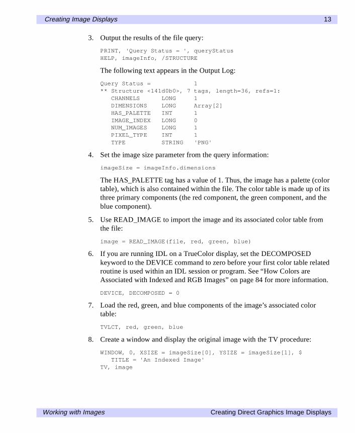
9. Use the XLOADCT utility to display the associated color table:
XLOADCT
Click on the Done button of XLOADCT to exit out of the utility.
The following figure shows the resulting indexed image and its color table.
The data values within the image are indexed to specific colors within thetable. You can change the color table associated with this image to show howan indexed images is dependent upon its related color table.
10. Change the current color table to the EOS B pre-defined color table:
LOADCT, 27
11. Redisplay the image to show the color table change:
TV, image
NoteThis step is not always necessary to redisplay the image. On some computers, thedisplay will update automatically when the current color table is changed.
Figure 3: Indexed Image and Associated Color Table in Direct Graphics
Creating Direct Graphics Image Displays Working with Images
Creating Image Displays 15
imgdispl.fm Page 15 Wednesday, March 6, 2002 5:29 PM
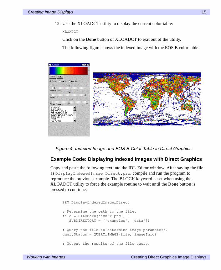
12. Use the XLOADCT utility to display the current color table:
XLOADCT
Click on the Done button of XLOADCT to exit out of the utility.
The following figure shows the indexed image with the EOS B color table.
Example Code: Displaying Indexed Images with Direct Graphics
Copy and paste the following text into the IDL Editor window. After saving the fileas DisplayIndexedImage_Direct.pro, compile and run the program toreproduce the previous example. The BLOCK keyword is set when using theXLOADCT utility to force the example routine to wait until the Done button ispressed to continue.
PRO DisplayIndexedImage_Direct
; Determine the path to the file.file = FILEPATH('avhrr.png', $
SUBDIRECTORY = ['examples', 'data'])
; Query the file to determine image parameters.queryStatus = QUERY_IMAGE(file, imageInfo)
; Output the results of the file query.
Figure 4: Indexed Image and EOS B Color Table in Direct Graphics
Working with Images Creating Direct Graphics Image Displays
16 Creating Image Displays
imgdispl.fm Page 16 Wednesday, March 6, 2002 5:29 PM
PRINT, 'Query Status = ', queryStatusHELP, imageInfo, /STRUCTURE
; Set image size parameter.imageSize = imageInfo.dimensions
; Import in the image and its associated color table; from the file.image = READ_IMAGE(file, red, green, blue)
; Initialize the display.DEVICE, DECOMPOSED = 0TVLCT, red, green, blue
; Create a window and display the image.WINDOW, 0, XSIZE = imageSize[0], YSIZE = imageSize[1], $
TITLE = 'An Indexed Image'TV, image
; Use the XLOADCT utility to display the color table.XLOADCT, /BLOCK
; Change the color table to the EOS B pre-defined color; table.LOADCT, 27
; Redisplay the image with the EOS B color table.TV, image
; Use the XLOADCT utility to display the current color; table.XLOADCT, /BLOCK
END
Displaying RGB Images with Direct Graphics
RGB images are three-dimensional arrays made up of width, height, and threechannels of color information. In Direct Graphics, these images are displayed withthe TV procedure. The TRUE keyword to TV is set according to the interleaving ofthe RGB image. With RGB images, the interleaving, or arrangement of the channelswithin the image file, dictates the setting of the TRUE keyword. If the image is:
• pixel interleaved (3, w, h), TRUE is set to 1.
• line interleaved (w, 3, h), TRUE is set to 2.
Creating Direct Graphics Image Displays Working with Images
Creating Image Displays 17
imgdispl.fm Page 17 Wednesday, March 6, 2002 5:29 PM
• image interleaved (w, h, 3), TRUE is set to 3.
You can determine if an image file contains an RGB image by querying the file. TheCHANNELS tag of the resulting query structure will equal 3 if the file’s image isRGB. The query does not determine which interleaving is used in the image, but thearray returned in DIMENSIONS tag of the query structure can be used to determinethe type of interleaving.
Unlike indexed images (two dimensional arrays with an associated color table), RGBimages contain their own color information. However, if you are using a PseudoColordisplay, your RGB images must be converted to indexed images to be displayedwithin IDL. See “How Colors are Associated with Indexed and RGB Images” onpage 84 for more information on RGB images and PseudoColor displays.
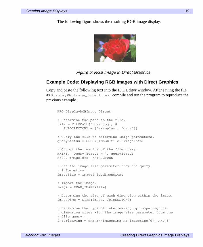
The following example queries and imports a pixel-interleaved RGB image from therose.jpg image file. This RGB image is a close-up photograph of a red rose. It ispixel interleaved.
For code that you can copy and paste into an Editor window, see “Example Code:Displaying RGB Images with Direct Graphics” on page 19 or complete the followingsteps for a detailed description of the process.
1. Determine the path to the rose.jpg file:
file = FILEPATH('rose.jpg', $SUBDIRECTORY = ['examples', 'data'])
2. Use QUERY_IMAGE to query the file to determine image parameters:
queryStatus = QUERY_IMAGE(file, imageInfo)
3. Output the results of the file query:
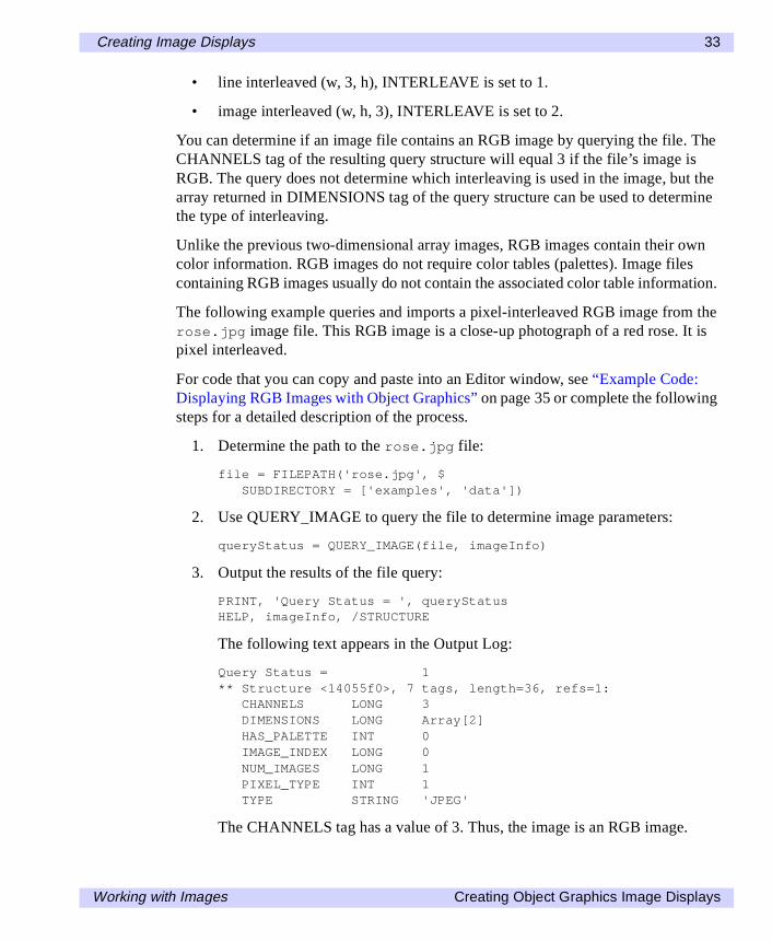
PRINT, 'Query Status = ', queryStatusHELP, imageInfo, /STRUCTURE
The following text appears in the Output Log:
Query Status = 1** Structure <14055f0>, 7 tags, length=36, refs=1:
CHANNELS LONG 3DIMENSIONS LONG Array[2]HAS_PALETTE INT 0IMAGE_INDEX LONG 0NUM_IMAGES LONG 1PIXEL_TYPE INT 1TYPE STRING 'JPEG'
The CHANNELS tag has a value of 3. Thus, the image is an RGB image.
Working with Images Creating Direct Graphics Image Displays
18 Creating Image Displays
imgdispl.fm Page 18 Wednesday, March 6, 2002 5:29 PM
4. Set the image size parameter from the query information:
imageSize = imageInfo.dimensions
The type of interleaving can be determined from the image size parameter andactual size of each dimension of the image. To determine the size of eachdimension, you must first import the image.
5. Use READ_IMAGE to import the image from the file:
image = READ_IMAGE(file)
6. Determine the size of each dimension within the image:
imageDims = SIZE(image, /DIMENSIONS)
7. Determine the type of interleaving by comparing the dimension sizes to theimage size parameter from the file query:
interleaving = WHERE((imageDims NE imageSize[0]) AND $(imageDims NE imageSize[1])) + 1
8. Output the results of the interleaving computation:
PRINT, 'Type of Interleaving = ', interleaving
The following text appears in the Output Log:
Type of Interleaving = 1
The image is pixel interleaved. If the resulting value was 2, the image wouldhave been line interleaved. If the resulting value was 3, the image would havebeen image interleaved.
9. If you are running IDL on a TrueColor display, set the DECOMPOSEDkeyword to the DEVICE command to one before your first RGB image isdisplayed within an IDL session or program. See “How Colors are Associatedwith Indexed and RGB Images” for more information:
DEVICE, DECOMPOSED = 1
10. Create a window and display the image with the TV procedure:
WINDOW, 0, XSIZE = imageSize[0], YSIZE = imageSize[1], $TITLE = 'An RGB Image'
TV, image, TRUE = interleaving[0]
Creating Direct Graphics Image Displays Working with Images
Creating Image Displays 19
imgdispl.fm Page 19 Wednesday, March 6, 2002 5:29 PM
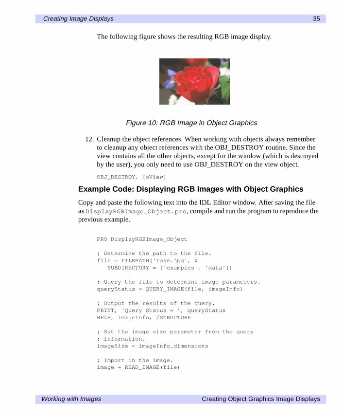
The following figure shows the resulting RGB image display.
Example Code: Displaying RGB Images with Direct Graphics
Copy and paste the following text into the IDL Editor window. After saving the fileas DisplayRGBImage_Direct.pro, compile and run the program to reproduce theprevious example.
PRO DisplayRGBImage_Direct
; Determine the path to the file.file = FILEPATH('rose.jpg', $
SUBDIRECTORY = ['examples', 'data'])
; Query the file to determine image parameters.queryStatus = QUERY_IMAGE(file, imageInfo)
; Output the results of the file query.PRINT, 'Query Status = ', queryStatusHELP, imageInfo, /STRUCTURE
; Set the image size parameter from the query; information.imageSize = imageInfo.dimensions
; Import the image.image = READ_IMAGE(file)
; Determine the size of each dimension within the image.imageDims = SIZE(image, /DIMENSIONS)
; Determine the type of interleaving by comparing the; dimension sizes with the image size parameter from the; file query.interleaving = WHERE((imageDims NE imageSize[0]) AND $
Figure 5: RGB Image in Direct Graphics
Working with Images Creating Direct Graphics Image Displays
20 Creating Image Displays
imgdispl.fm Page 20 Wednesday, March 6, 2002 5:29 PM
(imageDims NE imageSize[1])) + 1
; Output the results of the interleaving computation.PRINT, 'Type of Interleaving = ', interleaving
; Initialize display.DEVICE, DECOMPOSED = 1
; Create a window and display the image with the TV; procedure and its TRUE keyword.WINDOW, 0, XSIZE = imageSize[0], YSIZE = imageSize[1], $
TITLE = 'An RGB Image'TV, image, TRUE = interleaving[0]
END
Creating Direct Graphics Image Displays Working with Images
Creating Image Displays 21
imgdispl.fm Page 21 Wednesday, March 6, 2002 5:29 PM
Creating Object Graphics Image Displays
In Object Graphics, binary, grayscale, indexed, and RGB images are contained inimage objects. The image object is contained within a model object, which is a part ofa view object. The view object is displayed within a window object with the Drawmethod to that window object. For some types of images, their data values must bescaled with the BYTSCL function before displaying the image in a window object.When the scaling is required depends on the type of image to be displayed.
This section includes the following examples:
• “Displaying Binary Images with Object Graphics”.
• “Displaying Grayscale Images with Object Graphics” on page 24.
• “Displaying Indexed Images with Object Graphics” on page 27.
• “Displaying RGB images with Object Graphics” on page 32.
Displaying Binary Images with Object Graphics
Binary images are composed of pixels having one of two values, usually 0 or 1.These values are usually zero and one. With most color tables, pixels having valuesof zero and one are displayed with almost the same color, especially with a normalgrayscale color table. Thus, a binary image is usually scaled to display the zeros asblack and the ones as white.
The following example imports a binary image of the world from thecontinent_mask.dat binary file. In this image, the oceans are zeros (black) andthe continents are ones (white). This type of image can be used to mask out (omit)data over the oceans. The image contains byte data values and is 360 pixels by 360pixels.
For code that you can copy and paste into an Editor window, see “Example Code:Displaying Binary Images with Object Graphics” on page 23 or complete thefollowing steps for a detailed description of the process.
1. Determine the path to the continent_mask.dat file:
file = FILEPATH('continent_mask.dat', $SUBDIRECTORY = ['examples', 'data'])
2. Initialize the image size parameter:
imageSize = [360, 360]
Working with Images Creating Object Graphics Image Displays
22 Creating Image Displays
imgdispl.fm Page 22 Wednesday, March 6, 2002 5:29 PM
3. Use READ_BINARY to import the image from the file:
image = READ_BINARY(file, DATA_DIMS = imageSize)
4. Initialize the display objects:
oWindow = OBJ_NEW('IDLgrWindow', RETAIN = 2, $DIMENSIONS = imageSize, $TITLE = 'A Binary Image, Not Scaled')
oView = OBJ_NEW('IDLgrView', $VIEWPLANE_RECT = [0., 0., imageSize])
oModel = OBJ_NEW('IDLgrModel')
5. Initialize the image object:
oImage = OBJ_NEW('IDLgrImage', image)
6. Add the image object to the model, which is added to the view, then display theview in the window:
oModel -> Add, oImageoView -> Add, oModeloWindow -> Draw, oView
The resulting window should be all black (blank). The binary image containszeros and ones, which are almost the same color (black). A binary imageshould be scaled prior to displaying in order to show the ones as white.
7. Initialize another window:
oWindow = OBJ_NEW('IDLgrWindow', RETAIN = 2, $DIMENSIONS = imageSize, $TITLE = 'A Binary Image, Scaled')
8. Update the image object with a scaled version of the image:
oImage -> SetProperty, DATA = BYTSCL(image)
9. Display the view in the window:
oWindow -> Draw, oView
Creating Object Graphics Image Displays Working with Images
Creating Image Displays 23
imgdispl.fm Page 23 Wednesday, March 6, 2002 5:29 PM
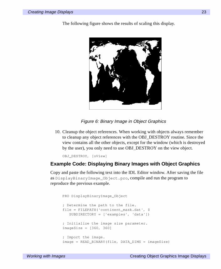
The following figure shows the results of scaling this display.
10. Cleanup the object references. When working with objects always rememberto cleanup any object references with the OBJ_DESTROY routine. Since theview contains all the other objects, except for the window (which is destroyedby the user), you only need to use OBJ_DESTROY on the view object.
OBJ_DESTROY, [oView]
Example Code: Displaying Binary Images with Object Graphics
Copy and paste the following text into the IDL Editor window. After saving the fileas DisplayBinaryImage_Object.pro, compile and run the program toreproduce the previous example.
PRO DisplayBinaryImage_Object
; Determine the path to the file.file = FILEPATH('continent_mask.dat', $
SUBDIRECTORY = ['examples', 'data'])
; Initialize the image size parameter.imageSize = [360, 360]
; Import the image.image = READ_BINARY(file, DATA_DIMS = imageSize)
Figure 6: Binary Image in Object Graphics
Working with Images Creating Object Graphics Image Displays
24 Creating Image Displays
imgdispl.fm Page 24 Wednesday, March 6, 2002 5:29 PM
; Initialize display objects.oWindow = OBJ_NEW('IDLgrWindow', RETAIN = 2, $
DIMENSIONS = imageSize, $TITLE = 'A Binary Image, Not Scaled')
oView = OBJ_NEW('IDLgrView', $VIEWPLANE_RECT = [0., 0., imageSize])
oModel = OBJ_NEW('IDLgrModel')
; Initialize image object.oImage = OBJ_NEW('IDLgrImage', image)
; Add the image to the model, which is added to the; view, and then display the view in the window.oModel -> Add, oImageoView -> Add, oModeloWindow -> Draw, oView
; Initialize another window.oWindow = OBJ_NEW('IDLgrWindow', RETAIN = 2, $
DIMENSIONS = imageSize, $TITLE = 'A Binary Image, Scaled')
; Update the image object with a scaled version of the; image.oImage -> SetProperty, DATA = BYTSCL(image)
; Display the view in the window.oWindow -> Draw, oView
; Cleanup object references.OBJ_DESTROY, [oView]
END
Displaying Grayscale Images with Object Graphics
Features within grayscale images are created by pixels that have varying intensities.Pixel values range from least intense (black) to the most instance (white). Since agrayscale image is composed of pixels of varying intensities, it is best displayed witha color table that progresses linearly from black to white. IDL provides several pre-defined color tables that progress linearly from black to white, but the bestrepresentation of a grayscale image is still the normal grayscale color table, which isthe default palette for IDL Object Graphics.
Creating Object Graphics Image Displays Working with Images
Creating Image Displays 25
imgdispl.fm Page 25 Wednesday, March 6, 2002 5:29 PM
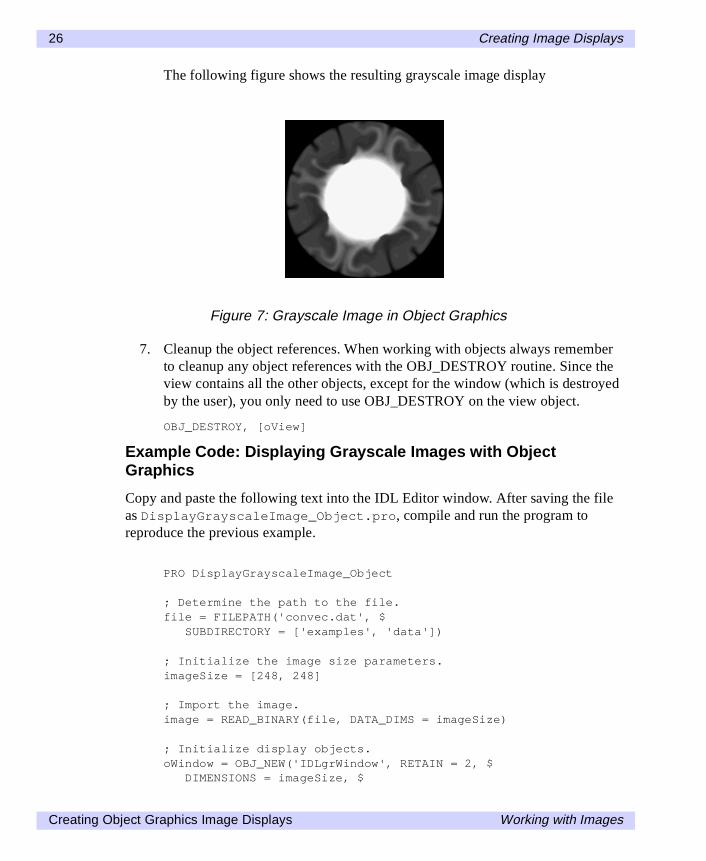
The following example imports a grayscale image from the convec.dat binary file.This grayscale image shows the convection of the Earth’s mantle. The image containsbyte data values and is 248 pixels by 248 pixels. Since the data type is byte, thisimage does not need to by scaled before display. If the data was of any type other thanbyte and the data values were not within the range of 0 up to 255, the display wouldneed to scale the image in order to show its intensities.
For code that you can copy and paste into an Editor window, see “Example Code:Displaying Grayscale Images with Object Graphics” on page 26 or complete thefollowing steps for a detailed description of the process.
1. Determine the path to the convec.dat file:
file = FILEPATH('convec.dat', $SUBDIRECTORY = ['examples', 'data'])
2. Initialize the image size parameter:
imageSize = [248, 248]
3. Using READ_BINARY, import the image from the file:
image = READ_BINARY(file, DATA_DIMS = imageSize)
4. Initialize the display objects:
oWindow = OBJ_NEW('IDLgrWindow', RETAIN = 2, $DIMENSIONS = imageSize, $TITLE = 'A Grayscale Image')
oView = OBJ_NEW('IDLgrView', $VIEWPLANE_RECT = [0., 0., imageSize])
oModel = OBJ_NEW('IDLgrModel')
5. Initialize the image object:
oImage = OBJ_NEW('IDLgrImage', image, /GREYSCALE)
6. Add the image object to the model, which is added to the view, then display theview in the window:
oModel -> Add, oImageoView -> Add, oModeloWindow -> Draw, oView
Working with Images Creating Object Graphics Image Displays
26 Creating Image Displays
imgdispl.fm Page 26 Wednesday, March 6, 2002 5:29 PM
The following figure shows the resulting grayscale image display
7. Cleanup the object references. When working with objects always rememberto cleanup any object references with the OBJ_DESTROY routine. Since theview contains all the other objects, except for the window (which is destroyedby the user), you only need to use OBJ_DESTROY on the view object.
OBJ_DESTROY, [oView]
Example Code: Displaying Grayscale Images with ObjectGraphics
Copy and paste the following text into the IDL Editor window. After saving the fileas DisplayGrayscaleImage_Object.pro, compile and run the program toreproduce the previous example.
PRO DisplayGrayscaleImage_Object
; Determine the path to the file.file = FILEPATH('convec.dat', $
SUBDIRECTORY = ['examples', 'data'])
; Initialize the image size parameters.imageSize = [248, 248]
; Import the image.image = READ_BINARY(file, DATA_DIMS = imageSize)
; Initialize display objects.oWindow = OBJ_NEW('IDLgrWindow', RETAIN = 2, $
DIMENSIONS = imageSize, $
Figure 7: Grayscale Image in Object Graphics
Creating Object Graphics Image Displays Working with Images
Creating Image Displays 27
imgdispl.fm Page 27 Wednesday, March 6, 2002 5:29 PM
TITLE = 'A Grayscale Image')oView = OBJ_NEW('IDLgrView', $
VIEWPLANE_RECT = [0., 0., imageSize])oModel = OBJ_NEW('IDLgrModel')
; Initialize image object.oImage = OBJ_NEW('IDLgrImage', image, $
/GREYSCALE)
; Add the image object to the model, which is added to; the view, then display the view in the window.oModel -> Add, oImageoView -> Add, oModeloWindow -> Draw, oView
; Cleanup object references.OBJ_DESTROY, [oView]
END
Displaying Indexed Images with Object Graphics
An indexed image contains up to 256 colors, typically defined by a color tableassociated with the image. The value of each pixel relates to a color within theassociated color table. Combinations of the primary colors (red, green, and blue)make up the colors within the color table. Indexed images are usually stored in imagefiles, instead of binary files, since they typically contain related color information (anassociated color table). You can query an image file to determine if it contains anindexed image.
The following example imports an indexed image from the avhrr.png image file.This indexed image is a satellite photograph of the world. Most indexed images rangein value from 0 up to 255 because of the range of the associated color table.Therefore, most indexed images do not require scaled displays.
For code that you can copy and paste into an Editor window, see “Example Code:Displaying Indexed Images with Object Graphics” on page 31 or complete thefollowing steps for a detailed description of the process.
1. Determine the path to the avhrr.png file:
file = FILEPATH('avhrr.png', $SUBDIRECTORY = ['examples', 'data'])
2. Use QUERY_IMAGE to query the file to determine image parameters:
queryStatus = QUERY_IMAGE(file, imageInfo)
Working with Images Creating Object Graphics Image Displays
28 Creating Image Displays
imgdispl.fm Page 28 Wednesday, March 6, 2002 5:29 PM
3. Output the results of the file query:
PRINT, 'Query Status = ', queryStatusHELP, imageInfo, /STRUCTURE
The following text appears in the Output Log:
Query Status = 1** Structure <141d0b0>, 7 tags, length=36, refs=1:
CHANNELS LONG 1DIMENSIONS LONG Array[2]HAS_PALETTE INT 1IMAGE_INDEX LONG 0NUM_IMAGES LONG 1PIXEL_TYPE INT 1TYPE STRING 'PNG'
4. Set the image size parameter from the query information:
imageSize = imageInfo.dimensions
The HAS_PALETTE tag has a value of 1. Thus, the image has a palette (colortable), which is also contained within the file. The color table is made up of itsthree primary components (the red component, the green component, and theblue component).
5. Use READ_IMAGE to import the image and its associated color table fromthe file:
image = READ_IMAGE(file, red, green, blue)
6. Initialize the display objects:
oWindow = OBJ_NEW('IDLgrWindow', RETAIN = 2, $DIMENSIONS = imageSize, TITLE = 'An Indexed Image')
oView = OBJ_NEW('IDLgrView', $VIEWPLANE_RECT = [0., 0., imageSize])
oModel = OBJ_NEW('IDLgrModel')
7. Initialize the image’s palette object:
oPalette = OBJ_NEW('IDLgrPalette', red, green, blue)
8. Initialize the image object with the resulting palette object:
oImage = OBJ_NEW('IDLgrImage', image, $PALETTE = oPalette)
Creating Object Graphics Image Displays Working with Images
Creating Image Displays 29
imgdispl.fm Page 29 Wednesday, March 6, 2002 5:29 PM
9. Add the image object to the model, which is added to the view, then display theview in the window:
oModel -> Add, oImageoView -> Add, oModeloWindow -> Draw, oView
10. Use the colorbar object to display the associated color table in anotherwindow:
oCbWindow = OBJ_NEW('IDLgrWindow', RETAIN = 2, $DIMENSIONS = [256, 48], $TITLE = 'Original Color Table')
oCbView = OBJ_NEW('IDLgrView', $VIEWPLANE_RECT = [0., 0., 256., 48.])
oCbModel = OBJ_NEW('IDLgrModel')oColorbar = OBJ_NEW('IDLgrColorbar', PALETTE = oPalette, $
DIMENSIONS = [256, 16], SHOW_AXIS = 1)oCbModel -> Add, oColorbaroCbView -> Add, oCbModeloCbWindow -> Draw, oCbView
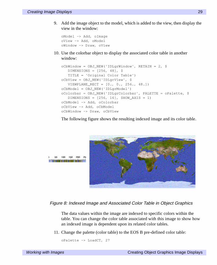
The following figure shows the resulting indexed image and its color table.
The data values within the image are indexed to specific colors within thetable. You can change the color table associated with this image to show howan indexed image is dependent upon its related color tables.
11. Change the palette (color table) to the EOS B pre-defined color table:
oPalette -> LoadCT, 27
Figure 8: Indexed Image and Associated Color Table in Object Graphics
Working with Images Creating Object Graphics Image Displays
30 Creating Image Displays
imgdispl.fm Page 30 Wednesday, March 6, 2002 5:29 PM
12. Redisplay the image in another window to show the palette change:
oWindow = OBJ_NEW('IDLgrWindow', RETAIN = 2, $DIMENSIONS = imageSize, TITLE = 'An Indexed Image')
oWindow -> Draw, oView
13. Redisplay the colorbar in another window to show the palette change:
oCbWindow = OBJ_NEW('IDLgrWindow', RETAIN = 2, $DIMENSIONS = [256, 48], $TITLE = 'EOS B Color Table')
oCbWindow -> Draw, oCbView
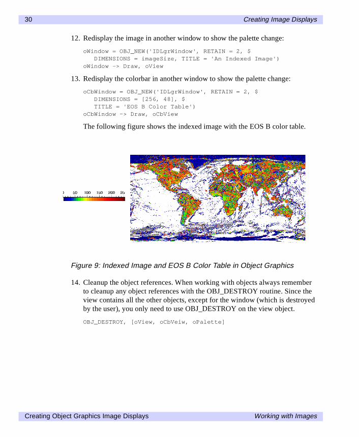
The following figure shows the indexed image with the EOS B color table.
14. Cleanup the object references. When working with objects always rememberto cleanup any object references with the OBJ_DESTROY routine. Since theview contains all the other objects, except for the window (which is destroyedby the user), you only need to use OBJ_DESTROY on the view object.
OBJ_DESTROY, [oView, oCbVeiw, oPalette]
Figure 9: Indexed Image and EOS B Color Table in Object Graphics
Creating Object Graphics Image Displays Working with Images
Creating Image Displays 31
imgdispl.fm Page 31 Wednesday, March 6, 2002 5:29 PM
Example Code: Displaying Indexed Images with Object Graphics
Copy and paste the following text into the IDL Editor window. After saving the fileas DisplayIndexedImage_Object.pro, compile and run the program toreproduce the previous example.
PRO DisplayIndexedImage_Object
; Determine the path to the file.file = FILEPATH('avhrr.png', $
SUBDIRECTORY = ['examples', 'data'])
; Query the file to determine image parameters.queryStatus = QUERY_IMAGE(file, imageInfo)
; Output the results of the query.PRINT, 'Query Status = ', queryStatusHELP, imageInfo, /STRUCTURE
; Set the image size parameter.imageSize = imageInfo.dimensions
; Import in the image.image = READ_IMAGE(file, red, green, blue)
; Initialize the display objects.oWindow = OBJ_NEW('IDLgrWindow', RETAIN = 2, $
DIMENSIONS = imageSize, TITLE = 'An Indexed Image')oView = OBJ_NEW('IDLgrView', $
VIEWPLANE_RECT = [0., 0., imageSize])oModel = OBJ_NEW('IDLgrModel')
; Initialize the image's palette object.oPalette = OBJ_NEW('IDLgrPalette', red, green, blue)
; Initialize the image object with the resulting; palette object.oImage = OBJ_NEW('IDLgrImage', image, $
PALETTE = oPalette)
; Add the image object to the model, which is added to; the view, then display the view in the window.oModel -> Add, oImageoView -> Add, oModeloWindow -> Draw, oView
; Use the colorbar object to display the associated; color table in another window.
Working with Images Creating Object Graphics Image Displays
32 Creating Image Displays
imgdispl.fm Page 32 Wednesday, March 6, 2002 5:29 PM
oCbWindow = OBJ_NEW('IDLgrWindow', RETAIN = 2, $DIMENSIONS = [256, 48], $TITLE = 'Original Color Table')
oCbView = OBJ_NEW('IDLgrView', $VIEWPLANE_RECT = [0., 0., 256., 48.])
oCbModel = OBJ_NEW('IDLgrModel')oColorbar = OBJ_NEW('IDLgrColorbar', PALETTE = oPalette, $
DIMENSIONS = [256, 16], SHOW_AXIS = 1)oCbModel -> Add, oColorbaroCbView -> Add, oCbModeloCbWindow -> Draw, oCbView
; Change the palette (color table) to the EOS B; pre-defined color table.oPalette -> LoadCT, 27
; Redisplay the image with the other color table in; another window.oWindow = OBJ_NEW('IDLgrWindow', RETAIN = 2, $
DIMENSIONS = imageSize, TITLE = 'An Indexed Image')oWindow -> Draw, oView
; Redisplay the colorbar with the other color table; in another window.oCbWindow = OBJ_NEW('IDLgrWindow', RETAIN = 2, $
DIMENSIONS = [256, 48], $TITLE = 'EOS B Color Table')
oCbWindow -> Draw, oCbView
; Cleanup object references.OBJ_DESTROY, [oView, oCbView, oPalette]
END
Displaying RGB images with Object Graphics
RGB images are three-dimensional arrays. In Object Graphics, an RGB image iscontained within an image object. An image object is contained within a modelobject, which is a part of a view object. The view object is displayed within a windowobject with the Draw method to that window object.
The INTERLEAVE keyword to the Init method of the image object is used whendisplaying an RGB image. With RGB images, the interleaving, or arrangement of thechannels within the image file, dictates the setting of the INTERLEAVE keyword. Ifthe image is:
• pixel interleaved (3, w, h), INTERLEAVE is set to 0.
Creating Object Graphics Image Displays Working with Images
Creating Image Displays 33
imgdispl.fm Page 33 Wednesday, March 6, 2002 5:29 PM
• line interleaved (w, 3, h), INTERLEAVE is set to 1.
• image interleaved (w, h, 3), INTERLEAVE is set to 2.
You can determine if an image file contains an RGB image by querying the file. TheCHANNELS tag of the resulting query structure will equal 3 if the file’s image isRGB. The query does not determine which interleaving is used in the image, but thearray returned in DIMENSIONS tag of the query structure can be used to determinethe type of interleaving.
Unlike the previous two-dimensional array images, RGB images contain their owncolor information. RGB images do not require color tables (palettes). Image filescontaining RGB images usually do not contain the associated color table information.
The following example queries and imports a pixel-interleaved RGB image from therose.jpg image file. This RGB image is a close-up photograph of a red rose. It ispixel interleaved.
For code that you can copy and paste into an Editor window, see “Example Code:Displaying RGB Images with Object Graphics” on page 35 or complete the followingsteps for a detailed description of the process.
1. Determine the path to the rose.jpg file:
file = FILEPATH('rose.jpg', $SUBDIRECTORY = ['examples', 'data'])
2. Use QUERY_IMAGE to query the file to determine image parameters:
queryStatus = QUERY_IMAGE(file, imageInfo)
3. Output the results of the file query:
PRINT, 'Query Status = ', queryStatusHELP, imageInfo, /STRUCTURE
The following text appears in the Output Log:
Query Status = 1** Structure <14055f0>, 7 tags, length=36, refs=1:
CHANNELS LONG 3DIMENSIONS LONG Array[2]HAS_PALETTE INT 0IMAGE_INDEX LONG 0NUM_IMAGES LONG 1PIXEL_TYPE INT 1TYPE STRING 'JPEG'
The CHANNELS tag has a value of 3. Thus, the image is an RGB image.
Working with Images Creating Object Graphics Image Displays
34 Creating Image Displays
imgdispl.fm Page 34 Wednesday, March 6, 2002 5:29 PM
4. Set the image size parameter from the query information:
imageSize = imageInfo.dimensions
The type of interleaving can be determined from the image size parameter andactual size of each dimension of the image. To determine the size of eachdimension, you must first import the image.
5. Use READ_IMAGE to import the image from the file:
image = READ_IMAGE(file)
6. Determine the size of each dimension within the image:
imageDims = SIZE(image, /DIMENSIONS)
7. Determine the type of interleaving by comparing the dimension sizes to theimage size parameter from the file query:
interleaving = WHERE((imageDims NE imageSize[0]) AND $(imageDims NE imageSize[1]))
8. Output the results of the interleaving computation:
PRINT, 'Type of Interleaving = ', interleaving
The following text appears in the Output Log:
Type of Interleaving = 0
The image is pixel interleaved. If the resulting value was 1, the image wouldhave been line interleaved. If the resulting value was 2, the image would havebeen image interleaved.
9. Initialize the display objects:
oWindow = OBJ_NEW('IDLgrWindow', RETAIN = 2, $DIMENSIONS = imageSize, TITLE = 'An RGB Image')
oView = OBJ_NEW('IDLgrView', $VIEWPLANE_RECT = [0., 0., imageSize])
oModel = OBJ_NEW('IDLgrModel')
10. Initialize the image object:
oImage = OBJ_NEW('IDLgrImage', image, $INTERLEAVE = interleaving[0])
11. Add the image object to the model, which is added to the view, then display theview in the window:
oModel -> Add, oImageoView -> Add, oModeloWindow -> Draw, oView
Creating Object Graphics Image Displays Working with Images
Creating Image Displays 35
imgdispl.fm Page 35 Wednesday, March 6, 2002 5:29 PM
The following figure shows the resulting RGB image display.
12. Cleanup the object references. When working with objects always rememberto cleanup any object references with the OBJ_DESTROY routine. Since theview contains all the other objects, except for the window (which is destroyedby the user), you only need to use OBJ_DESTROY on the view object.
OBJ_DESTROY, [oView]
Example Code: Displaying RGB Images with Object Graphics
Copy and paste the following text into the IDL Editor window. After saving the fileas DisplayRGBImage_Object.pro, compile and run the program to reproduce theprevious example.
PRO DisplayRGBImage_Object
; Determine the path to the file.file = FILEPATH('rose.jpg', $
SUBDIRECTORY = ['examples', 'data'])
; Query the file to determine image parameters.queryStatus = QUERY_IMAGE(file, imageInfo)
; Output the results of the query.PRINT, 'Query Status = ', queryStatusHELP, imageInfo, /STRUCTURE
; Set the image size parameter from the query; information.imageSize = imageInfo.dimensions
; Import in the image.image = READ_IMAGE(file)
Figure 10: RGB Image in Object Graphics
Working with Images Creating Object Graphics Image Displays
36 Creating Image Displays
imgdispl.fm Page 36 Wednesday, March 6, 2002 5:29 PM
; Determine the size of each dimension within the image.imageDims = SIZE(image, /DIMENSIONS)
; Determine the type of interleaving by comparing; dimension size and the size of the image.interleaving = WHERE((imageDims NE imageSize[0]) AND $
(imageDims NE imageSize[1]))
; Output the results of the interleaving computation.PRINT, 'Type of Interleaving = ', interleaving
; Initialize the display objects.oWindow = OBJ_NEW('IDLgrWindow', RETAIN = 2, $
DIMENSIONS = imageSize, TITLE = 'An RGB Image')oView = OBJ_NEW('IDLgrView', $
VIEWPLANE_RECT = [0., 0., imageSize])oModel = OBJ_NEW('IDLgrModel')
; Initialize the image object.oImage = OBJ_NEW('IDLgrImage', image, $
INTERLEAVE = interleaving[0])
; Add the image object to the model, which is added to; the view, then display the view in the window.oModel -> Add, oImageoView -> Add, oModeloWindow -> Draw, oView
; Cleanup object references.OBJ_DESTROY, [oView]
END
Creating Object Graphics Image Displays Working with Images
Creating Image Displays 37
imgdispl.fm Page 37 Wednesday, March 6, 2002 5:29 PM
Displaying Multiple Images in a Window
How multiple images are displayed in a single window depends upon which graphicssystem is being used to display the images. Direct Graphics uses location inputarguments for the TV procedure to position images in a window, see “DisplayingMultiple Images in Direct Graphics” for more information. Object Graphics used theLOCATION keyword to the Init method of the image object to position images in awindow, see “Displaying Multiple Images in Object Graphics” on page 42 for moreinformation.
Displaying Multiple Images in Direct Graphics
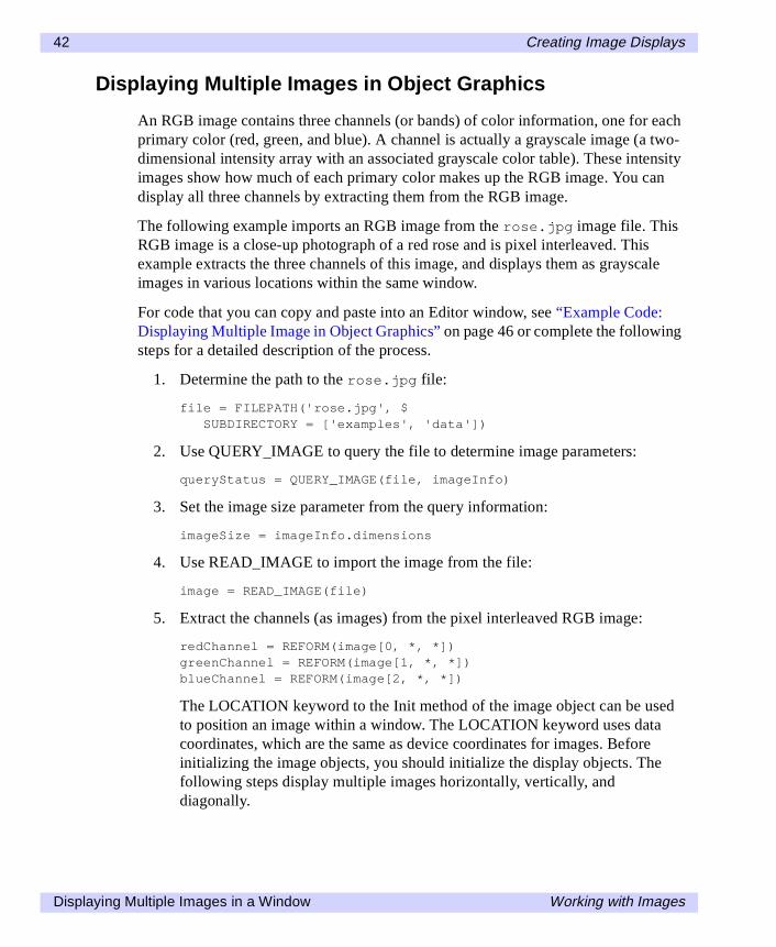
An RGB image contains three channels (or bands) of color information, one for eachprimary color (red, green, and blue). A channel is actually a grayscale image (a two-dimensional intensity array with an associated grayscale color table). These intensityimages show how much of each primary color makes up the RGB image. You candisplay all three channels by extracting them from the RGB image.
The following example imports an RGB image from the rose.jpg image file. ThisRGB image is a close-up photograph of a red rose and is pixel interleaved. Thisexample extracts the three channels of this image, and displays them as grayscaleimages in various locations within the same window.
For code that you can copy and paste into an Editor window, see “Example Code:Displaying Multiple Image in Direct Graphics” on page 40 or complete the followingsteps for a detailed description of the process.
1. Determine the path to the rose.jpg file:
file = FILEPATH('rose.jpg', $SUBDIRECTORY = ['examples', 'data'])
2. Use QUERY_IMAGE to query the file to determine image parameters:
queryStatus = QUERY_IMAGE(file, imageInfo)
3. Set the image size parameter from the query information:
imageSize = imageInfo.dimensions
4. Use READ_IMAGE to import the image from the file:
image = READ_IMAGE(file)
Working with Images Displaying Multiple Images in a Window
38 Creating Image Displays
imgdispl.fm Page 38 Wednesday, March 6, 2002 5:29 PM
5. Extract the channels (as images) from the pixel interleaved RGB image:
redChannel = REFORM(image[0, *, *])greenChannel = REFORM(image[1, *, *])blueChannel = REFORM(image[2, *, *])
6. If you are running IDL on a TrueColor display, set the DECOMPOSEDkeyword to the DEVICE command to zero before your first color table relatedroutine is used within an IDL session or program. See “How Colors areAssociated with Indexed and RGB Images” for more information.
DEVICE, DECOMPOSED = 0
7. Since the channels are grayscale images, load a grayscale color table:
LOADCT, 0
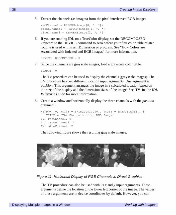
The TV procedure can be used to display the channels (grayscale images). TheTV procedure has two different location input arguments. One argument isposition. This argument arranges the image in a calculated location based onthe size of the display and the dimension sizes of the image. See TV in the IDLReference Guide for more information.
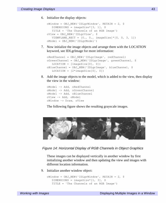
8. Create a window and horizontally display the three channels with the positionargument:
WINDOW, 0, XSIZE = 3*imageSize[0], YSIZE = imageSize[1], $TITLE = 'The Channels of an RGB Image'
TV, redChannel, 0TV, greenChannel, 1TV, blueChannel, 2
The following figure shows the resulting grayscale images.
The TV procedure can also be used with its x and y input arguments. Thesearguments define the location of the lower left corner of the image. The valuesof these arguments are in device coordinates by default. However, you can
Figure 11: Horizontal Display of RGB Channels in Direct Graphics
Displaying Multiple Images in a Window Working with Images
Creating Image Displays 39
imgdispl.fm Page 39 Wednesday, March 6, 2002 5:29 PM
provide data or normalized coordinates when the DATA or NORMALkeyword is set. See TV in the IDL Reference Guide for more information.
9. Create a window and vertically display the three channels with the x and yarguments:
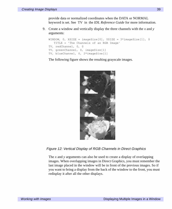
WINDOW, 0, XSIZE = imageSize[0], YSIZE = 3*imageSize[1], $TITLE = 'The Channels of an RGB Image'
TV, redChannel, 0, 0TV, greenChannel, 0, imageSize[1]TV, blueChannel, 0, 2*imageSize[1]
The following figure shows the resulting grayscale images.
The x and y arguments can also be used to create a display of overlappingimages. When overlapping images in Direct Graphics, you must remember thelast image placed in the window will be in front of the previous images. So ifyou want to bring a display from the back of the window to the front, you mustredisplay it after all the other displays.
Figure 12: Vertical Display of RGB Channels in Direct Graphics
Working with Images Displaying Multiple Images in a Window
40 Creating Image Displays
imgdispl.fm Page 40 Wednesday, March 6, 2002 5:29 PM
10. Create another window:
WINDOW, 2, XSIZE = 2*imageSize[0], YSIZE = 2*imageSize[1], $TITLE = 'The Channels of an RGB Image'
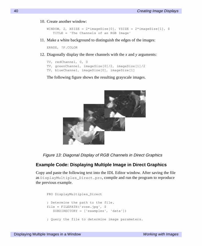
11. Make a white background to distinguish the edges of the images:
ERASE, !P.COLOR
12. Diagonally display the three channels with the x and y arguments:
TV, redChannel, 0, 0TV, greenChannel, imageSize[0]/2, imageSize[1]/2TV, blueChannel, imageSize[0], imageSize[1]
The following figure shows the resulting grayscale images.
Example Code: Displaying Multiple Image in Direct Graphics
Copy and paste the following text into the IDL Editor window. After saving the fileas DisplayMultiples_Direct.pro, compile and run the program to reproducethe previous example.
PRO DisplayMultiples_Direct
; Determine the path to the file.file = FILEPATH('rose.jpg', $
SUBDIRECTORY = ['examples', 'data'])
; Query the file to determine image parameters.
Figure 13: Diagonal Display of RGB Channels in Direct Graphics
Displaying Multiple Images in a Window Working with Images
Creating Image Displays 41
imgdispl.fm Page 41 Wednesday, March 6, 2002 5:29 PM
queryStatus = QUERY_IMAGE(file, imageInfo)
; Set the image size parameter from the query; information.imageSize = imageInfo.dimensions
; Import the image.image = READ_IMAGE(file)
; Extract the channels (as images) from the RGB image.redChannel = REFORM(image[0, *, *])greenChannel = REFORM(image[1, *, *])blueChannel = REFORM(image[2, *, *])
; Initialize displays.DEVICE, DECOMPOSED = 0LOADCT, 0
; Create a window and horizontally display the channels.WINDOW, 0, XSIZE = 3*imageSize[0], YSIZE = imageSize[1], $
TITLE = 'The Channels of an RGB Image'TV, redChannel, 0TV, greenChannel, 1TV, blueChannel, 2
; Create another window and vertically display the; channels.WINDOW, 1, XSIZE = imageSize[0], YSIZE = 3*imageSize[1], $
TITLE = 'The Channels of an RGB Image'TV, redChannel, 0, 0TV, greenChannel, 0, imageSize[1]TV, blueChannel, 0, 2*imageSize[1]
; Create another window.WINDOW, 2, XSIZE = 2*imageSize[0], YSIZE = 2*imageSize[1], $
TITLE = 'The Channels of an RGB Image'
; Make a white background.ERASE, !P.COLOR
; Diagonally display the channels.TV, redChannel, 0, 0TV, greenChannel, imageSize[0]/2, imageSize[1]/2TV, blueChannel, imageSize[0], imageSize[1]
END
Working with Images Displaying Multiple Images in a Window
42 Creating Image Displays
imgdispl.fm Page 42 Wednesday, March 6, 2002 5:29 PM
Displaying Multiple Images in Object Graphics
An RGB image contains three channels (or bands) of color information, one for eachprimary color (red, green, and blue). A channel is actually a grayscale image (a two-dimensional intensity array with an associated grayscale color table). These intensityimages show how much of each primary color makes up the RGB image. You candisplay all three channels by extracting them from the RGB image.
The following example imports an RGB image from the rose.jpg image file. ThisRGB image is a close-up photograph of a red rose and is pixel interleaved. Thisexample extracts the three channels of this image, and displays them as grayscaleimages in various locations within the same window.
For code that you can copy and paste into an Editor window, see “Example Code:Displaying Multiple Image in Object Graphics” on page 46 or complete the followingsteps for a detailed description of the process.
1. Determine the path to the rose.jpg file:
file = FILEPATH('rose.jpg', $SUBDIRECTORY = ['examples', 'data'])
2. Use QUERY_IMAGE to query the file to determine image parameters:
queryStatus = QUERY_IMAGE(file, imageInfo)
3. Set the image size parameter from the query information:
imageSize = imageInfo.dimensions
4. Use READ_IMAGE to import the image from the file:
image = READ_IMAGE(file)
5. Extract the channels (as images) from the pixel interleaved RGB image:
redChannel = REFORM(image[0, *, *])greenChannel = REFORM(image[1, *, *])blueChannel = REFORM(image[2, *, *])
The LOCATION keyword to the Init method of the image object can be usedto position an image within a window. The LOCATION keyword uses datacoordinates, which are the same as device coordinates for images. Beforeinitializing the image objects, you should initialize the display objects. Thefollowing steps display multiple images horizontally, vertically, anddiagonally.
Displaying Multiple Images in a Window Working with Images
Creating Image Displays 43
imgdispl.fm Page 43 Wednesday, March 6, 2002 5:29 PM
6. Initialize the display objects:
oWindow = OBJ_NEW('IDLgrWindow', RETAIN = 2, $DIMENSIONS = imageSize*[3, 1], $TITLE = 'The Channels of an RGB Image')
oView = OBJ_NEW('IDLgrView', $VIEWPLANE_RECT = [0., 0., imageSize]*[0, 0, 3, 1])
oModel = OBJ_NEW('IDLgrModel')
7. Now initialize the image objects and arrange them with the LOCATIONkeyword, see IDLgrImage for more information:
oRedChannel = OBJ_NEW('IDLgrImage', redChannel)oGreenChannel = OBJ_NEW('IDLgrImage', greenChannel, $
LOCATION = [imageSize[0], 0])oBlueChannel = OBJ_NEW('IDLgrImage', blueChannel, $
LOCATION = [2*imageSize[0], 0])
8. Add the image objects to the model, which is added to the view, then displaythe view in the window:
oModel -> Add, oRedChanneloModel -> Add, oGreenChanneloModel -> Add, oBlueChanneloView -> Add, oModeloWindow -> Draw, oView
The following figure shows the resulting grayscale images.
These images can be displayed vertically in another window by firstinitializing another window and then updating the view and images withdifferent location information.
9. Initialize another window object:
oWindow = OBJ_NEW('IDLgrWindow', RETAIN = 2, $DIMENSIONS = imageSize*[1, 3], $TITLE = 'The Channels of an RGB Image')
Figure 14: Horizontal Display of RGB Channels in Object Graphics
Working with Images Displaying Multiple Images in a Window
44 Creating Image Displays
imgdispl.fm Page 44 Wednesday, March 6, 2002 5:29 PM
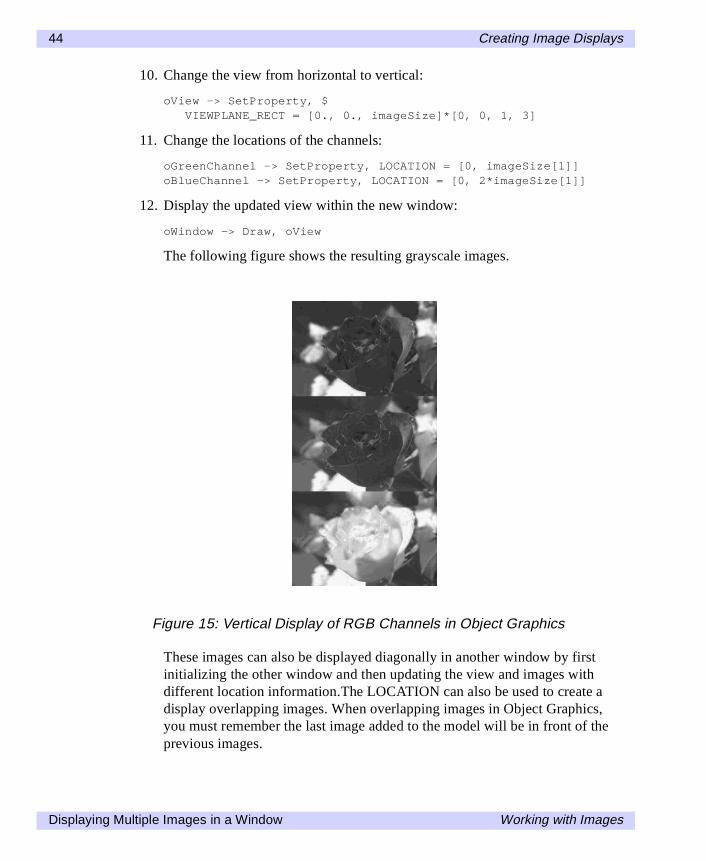
10. Change the view from horizontal to vertical:
oView -> SetProperty, $VIEWPLANE_RECT = [0., 0., imageSize]*[0, 0, 1, 3]
11. Change the locations of the channels:
oGreenChannel -> SetProperty, LOCATION = [0, imageSize[1]]oBlueChannel -> SetProperty, LOCATION = [0, 2*imageSize[1]]
12. Display the updated view within the new window:
oWindow -> Draw, oView
The following figure shows the resulting grayscale images.
These images can also be displayed diagonally in another window by firstinitializing the other window and then updating the view and images withdifferent location information.The LOCATION can also be used to create adisplay overlapping images. When overlapping images in Object Graphics,you must remember the last image added to the model will be in front of theprevious images.
Figure 15: Vertical Display of RGB Channels in Object Graphics
Displaying Multiple Images in a Window Working with Images
Creating Image Displays 45
imgdispl.fm Page 45 Wednesday, March 6, 2002 5:29 PM
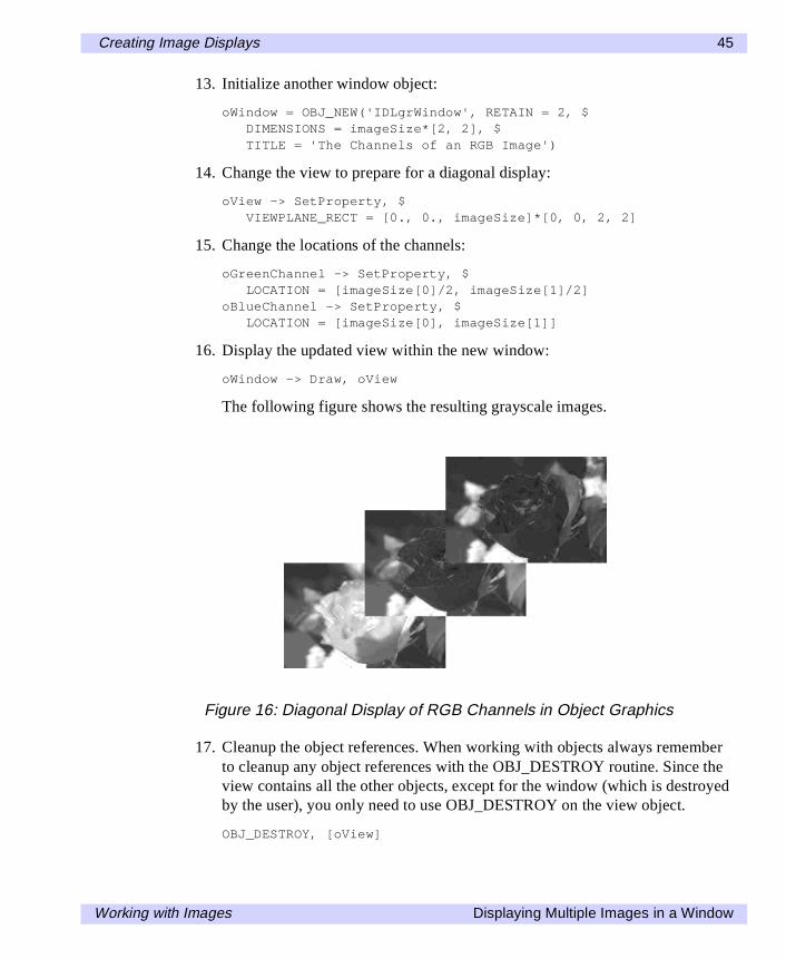
13. Initialize another window object:
oWindow = OBJ_NEW('IDLgrWindow', RETAIN = 2, $DIMENSIONS = imageSize*[2, 2], $TITLE = 'The Channels of an RGB Image')
14. Change the view to prepare for a diagonal display:
oView -> SetProperty, $VIEWPLANE_RECT = [0., 0., imageSize]*[0, 0, 2, 2]
15. Change the locations of the channels:
oGreenChannel -> SetProperty, $LOCATION = [imageSize[0]/2, imageSize[1]/2]
oBlueChannel -> SetProperty, $LOCATION = [imageSize[0], imageSize[1]]
16. Display the updated view within the new window:
oWindow -> Draw, oView
The following figure shows the resulting grayscale images.
17. Cleanup the object references. When working with objects always rememberto cleanup any object references with the OBJ_DESTROY routine. Since theview contains all the other objects, except for the window (which is destroyedby the user), you only need to use OBJ_DESTROY on the view object.
OBJ_DESTROY, [oView]
Figure 16: Diagonal Display of RGB Channels in Object Graphics
Working with Images Displaying Multiple Images in a Window
46 Creating Image Displays
imgdispl.fm Page 46 Wednesday, March 6, 2002 5:29 PM
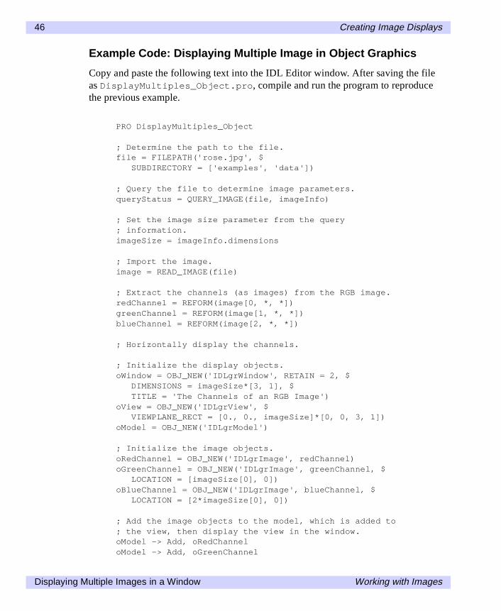
Example Code: Displaying Multiple Image in Object Graphics
Copy and paste the following text into the IDL Editor window. After saving the fileas DisplayMultiples_Object.pro, compile and run the program to reproducethe previous example.
PRO DisplayMultiples_Object
; Determine the path to the file.file = FILEPATH('rose.jpg', $
SUBDIRECTORY = ['examples', 'data'])
; Query the file to determine image parameters.queryStatus = QUERY_IMAGE(file, imageInfo)
; Set the image size parameter from the query; information.imageSize = imageInfo.dimensions
; Import the image.image = READ_IMAGE(file)
; Extract the channels (as images) from the RGB image.redChannel = REFORM(image[0, *, *])greenChannel = REFORM(image[1, *, *])blueChannel = REFORM(image[2, *, *])
; Horizontally display the channels.
; Initialize the display objects.oWindow = OBJ_NEW('IDLgrWindow', RETAIN = 2, $
DIMENSIONS = imageSize*[3, 1], $TITLE = 'The Channels of an RGB Image')
oView = OBJ_NEW('IDLgrView', $VIEWPLANE_RECT = [0., 0., imageSize]*[0, 0, 3, 1])
oModel = OBJ_NEW('IDLgrModel')
; Initialize the image objects.oRedChannel = OBJ_NEW('IDLgrImage', redChannel)oGreenChannel = OBJ_NEW('IDLgrImage', greenChannel, $
LOCATION = [imageSize[0], 0])oBlueChannel = OBJ_NEW('IDLgrImage', blueChannel, $
LOCATION = [2*imageSize[0], 0])
; Add the image objects to the model, which is added to; the view, then display the view in the window.oModel -> Add, oRedChanneloModel -> Add, oGreenChannel
Displaying Multiple Images in a Window Working with Images
Creating Image Displays 47
imgdispl.fm Page 47 Wednesday, March 6, 2002 5:29 PM
oModel -> Add, oBlueChanneloView -> Add, oModeloWindow -> Draw, oView
; Vertically display the channels.
; Initialize another window object.oWindow = OBJ_NEW('IDLgrWindow', RETAIN = 2, $
DIMENSIONS = imageSize*[1, 3], $TITLE = 'The Channels of an RGB Image')
; Change the view from horizontal to vertical.oView -> SetProperty, $
VIEWPLANE_RECT = [0., 0., imageSize]*[0, 0, 1, 3]
; Change the locations of the channels.oGreenChannel -> SetProperty, $
LOCATION = [0, imageSize[1]]oBlueChannel -> SetProperty, $
LOCATION = [0, 2*imageSize[1]]
; Display the updated view in the new window.oWindow -> Draw, oView
; Diagonally display the channels.
; Initialize another window object.oWindow = OBJ_NEW('IDLgrWindow', RETAIN = 2, $
DIMENSIONS = imageSize*[2, 2], $TITLE = 'The Channels of an RGB Image')
; Change the view from vertical to diagonal.oView -> SetProperty, $
VIEWPLANE_RECT = [0., 0., imageSize]*[0, 0, 2, 2]
; Change the locations of the channels.oGreenChannel -> SetProperty, $
LOCATION = [imageSize[0]/2, imageSize[1]/2]oBlueChannel -> SetProperty, $
LOCATION = [imageSize[0], imageSize[1]]
; Display the updated view in the new window.oWindow -> Draw, oView
; Cleanup object references.OBJ_DESTROY, [oView]
END
Working with Images Displaying Multiple Images in a Window
48 Creating Image Displays
imgdispl.fm Page 48 Wednesday, March 6, 2002 5:29 PM
Zooming in on an Image
Enlarging on a specific section of an image is known as zooming in on an image.How zooming is performed within IDL depends on the graphics system. In DirectGraphics, you can use the ZOOM procedure to zoom in on a specific section of animage, see “Zooming in on a Direct Graphics Image Display” for more information.If you are working with RGB images, you can use the ZOOM_24 procedure.
In Object Graphics, the VIEWPLANE_RECT keyword is used to change the viewobject. The entire image is still contained within the image object while the view ischanged to only show specific areas of the image object, see “Zooming in on a ObjectGraphics Image Display” on page 50 for more information.
Zooming in on a Direct Graphics Image Display
The following example imports a grayscale image from the convec.dat binary file.This grayscale image shows the convection of the Earth’s mantle. The image containsbyte data values and is 248 pixels by 248 pixels. The ZOOM procedure, which is aDirect Graphics routine, is used to zoom in on the lower left corner of the image.
For code that you can copy and paste into an Editor window, see “Example Code:Zooming in Direct Graphics” on page 50 or complete the following steps for adetailed description of the process.
1. Determine the path to the convec.dat file:
file = FILEPATH('convec.dat', $SUBDIRECTORY = ['examples', 'data'])
2. Initialize the image size parameter:
imageSize = [248, 248]
3. Import the image from the file:
image = READ_BINARY(file, DATA_DIMS = imageSize)
4. If you are running IDL on a TrueColor display, set the DECOMPOSEDkeyword to the DEVICE command to zero before your first color table relatedroutine is used within an IDL session or program. See “How Colors areAssociated with Indexed and RGB Images” for more information.
DEVICE, DECOMPOSED = 0
5. Load a grayscale color table:
LOADCT, 0
Zooming in on an Image Working with Images
Creating Image Displays 49
imgdispl.fm Page 49 Wednesday, March 6, 2002 5:29 PM
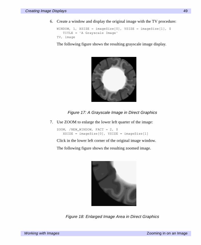
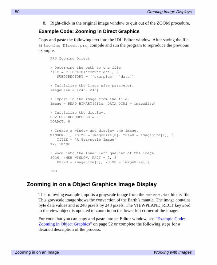
6. Create a window and display the original image with the TV procedure:
WINDOW, 1, XSIZE = imageSize[0], YSIZE = imageSize[1], $TITLE = 'A Grayscale Image'
TV, image
The following figure shows the resulting grayscale image display.
7. Use ZOOM to enlarge the lower left quarter of the image:
ZOOM, /NEW_WINDOW, FACT = 2, $XSIZE = imageSize[0], YSIZE = imageSize[1]
Click in the lower left corner of the original image window.
The following figure shows the resulting zoomed image.
Figure 17: A Grayscale Image in Direct Graphics
Figure 18: Enlarged Image Area in Direct Graphics
Working with Images Zooming in on an Image
50 Creating Image Displays
imgdispl.fm Page 50 Wednesday, March 6, 2002 5:29 PM
8. Right-click in the original image window to quit out of the ZOOM procedure.
Example Code: Zooming in Direct Graphics
Copy and paste the following text into the IDL Editor window. After saving the fileas Zooming_Direct.pro, compile and run the program to reproduce the previousexample.
PRO Zooming_Direct
; Determine the path to the file.file = FILEPATH('convec.dat', $
SUBDIRECTORY = ['examples', 'data'])
; Initialize the image size parameter.imageSize = [248, 248]
; Import in the image from the file.image = READ_BINARY(file, DATA_DIMS = imageSize)
; Initialize the display.DEVICE, DECOMPOSED = 0LOADCT, 0
; Create a window and display the image.WINDOW, 1, XSIZE = imageSize[0], YSIZE = imageSize[1], $
TITLE = 'A Grayscale Image'TV, image
; Zoom into the lower left quarter of the image.ZOOM, /NEW_WINDOW, FACT = 2, $
XSIZE = imageSize[0], YSIZE = imageSize[1]
END
Zooming in on a Object Graphics Image Display
The following example imports a grayscale image from the convec.dat binary file.This grayscale image shows the convection of the Earth’s mantle. The image containsbyte data values and is 248 pixels by 248 pixels. The VIEWPLANE_RECT keywordto the view object is updated to zoom in on the lower left corner of the image.
For code that you can copy and paste into an Editor window, see “Example Code:Zooming in Object Graphics” on page 52 or complete the following steps for adetailed description of the process.
Zooming in on an Image Working with Images
Creating Image Displays 51
imgdispl.fm Page 51 Wednesday, March 6, 2002 5:29 PM
1. Determine the path to the convec.dat file:
file = FILEPATH('convec.dat', $SUBDIRECTORY = ['examples', 'data'])
2. Initialize the image size parameter:
imageSize = [248, 248]
3. Import the image from the file:
image = READ_BINARY(file, DATA_DIMS = imageSize)
4. Initialize the display objects:
oWindow = OBJ_NEW('IDLgrWindow', RETAIN = 2, $DIMENSIONS = imageSize, $TITLE = 'A Grayscale Image')
oView = OBJ_NEW('IDLgrView', $VIEWPLANE_RECT = [0., 0., imageSize])
oModel = OBJ_NEW('IDLgrModel')
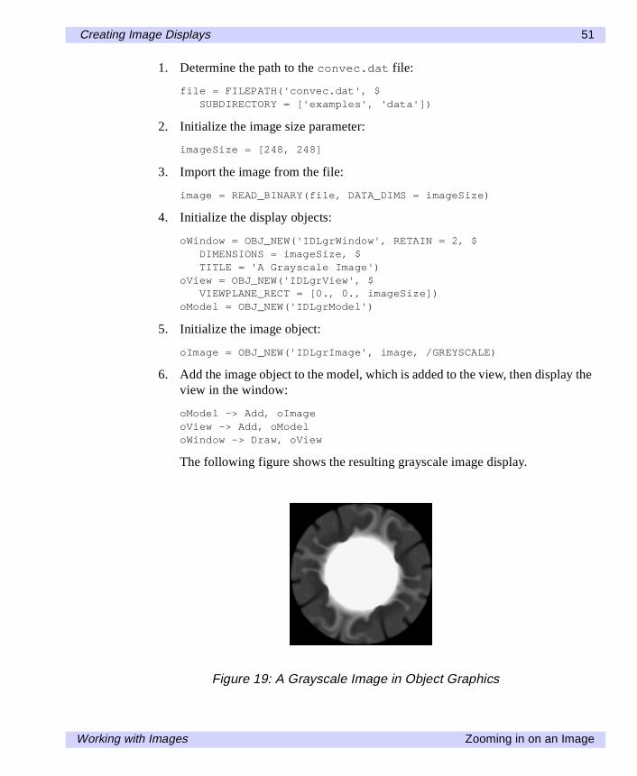
5. Initialize the image object:
oImage = OBJ_NEW('IDLgrImage', image, /GREYSCALE)
6. Add the image object to the model, which is added to the view, then display theview in the window:
oModel -> Add, oImageoView -> Add, oModeloWindow -> Draw, oView
The following figure shows the resulting grayscale image display.
Figure 19: A Grayscale Image in Object Graphics
Working with Images Zooming in on an Image
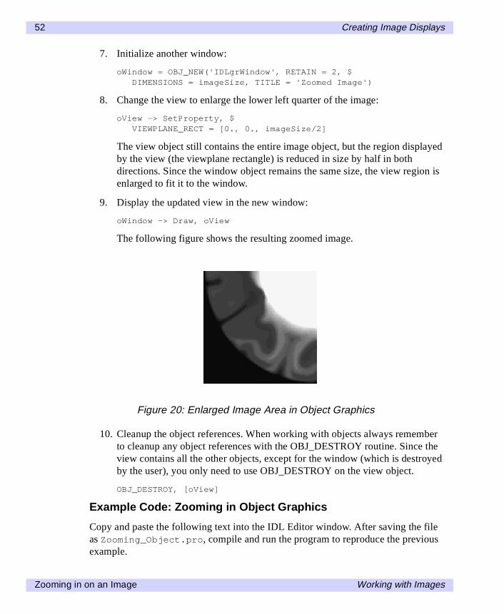
52 Creating Image Displays
imgdispl.fm Page 52 Wednesday, March 6, 2002 5:29 PM
7. Initialize another window:
oWindow = OBJ_NEW('IDLgrWindow', RETAIN = 2, $DIMENSIONS = imageSize, TITLE = 'Zoomed Image')
8. Change the view to enlarge the lower left quarter of the image:
oView -> SetProperty, $VIEWPLANE_RECT = [0., 0., imageSize/2]
The view object still contains the entire image object, but the region displayedby the view (the viewplane rectangle) is reduced in size by half in bothdirections. Since the window object remains the same size, the view region isenlarged to fit it to the window.
9. Display the updated view in the new window:
oWindow -> Draw, oView
The following figure shows the resulting zoomed image.
10. Cleanup the object references. When working with objects always rememberto cleanup any object references with the OBJ_DESTROY routine. Since theview contains all the other objects, except for the window (which is destroyedby the user), you only need to use OBJ_DESTROY on the view object.
OBJ_DESTROY, [oView]
Example Code: Zooming in Object Graphics
Copy and paste the following text into the IDL Editor window. After saving the fileas Zooming_Object.pro, compile and run the program to reproduce the previousexample.
Figure 20: Enlarged Image Area in Object Graphics
Zooming in on an Image Working with Images
Creating Image Displays 53
imgdispl.fm Page 53 Wednesday, March 6, 2002 5:29 PM
PRO Zooming_Object
; Determine the path to the file.file = FILEPATH('convec.dat', $
SUBDIRECTORY = ['examples', 'data'])
; Initialize the image size parameter.imageSize = [248, 248]
; Import in the image from the file.image = READ_BINARY(file, DATA_DIMS = imageSize)
; Initialize display objects.oWindow = OBJ_NEW('IDLgrWindow', RETAIN = 2, $
DIMENSIONS = imageSize, $TITLE = 'A Grayscale Image')
oView = OBJ_NEW('IDLgrView', $VIEWPLANE_RECT = [0., 0., imageSize])
oModel = OBJ_NEW('IDLgrModel')
; Initialize image object.oImage = OBJ_NEW('IDLgrImage', image, /GREYSCALE)
; Add the image object to the model, which is added to; the view, then display the view in the window.oModel -> Add, oImageoView -> Add, oModeloWindow -> Draw, oView
; Initialize another window.oWindow = OBJ_NEW('IDLgrWindow', RETAIN = 2, $
DIMENSIONS = imageSize, TITLE = 'Enlarged Area')
; Change view to zoom into the lower left quarter of; the image.oView -> SetProperty, $
VIEWPLANE_RECT = [0., 0., imageSize/2]
; Display updated view in new window.oWindow -> Draw, oView
; Cleanup object references.OBJ_DESTROY, [oView]
END
Working with Images Zooming in on an Image
54 Creating Image Displays
imgdispl.fm Page 54 Wednesday, March 6, 2002 5:29 PM
Panning within an Image
Panning involves moving an area of focus from one section of an image to othersections. How panning is performed within IDL depends on the graphics system. InDirect Graphics, you can use the SLIDE_IMAGE procedure to pan with sliders in anapplication that contains the image, see “Panning in Direct Graphics” for moreinformation.
In Object Graphics, the VIEWPLANE_RECT keyword is used to change the viewobject. The entire image is still contained within the image object, but the view ischanged to pan over specific areas of the image object, see “Panning in ObjectGraphics” on page 56 for more information.
Panning in Direct Graphics
The following example imports a grayscale image from the nyny.dat binary file.This grayscale image is an aerial view of New York City. The image contains bytedata values and is 768 pixels by 512 pixels. You can use the SLIDE_IMAGEprocedure to zoom in on the image and pan over it.
For code that you can copy and paste into an Editor window, see “Example Code:Panning in Direct Graphics” on page 55 or complete the following steps for a detaileddescription of the process.
1. Determine the path to the convec.dat file:
file = FILEPATH('nyny.dat', $SUBDIRECTORY = ['examples', 'data'])
2. Initialize the image size parameter:
imageSize = [768, 512]
3. Import the image from the file:
image = READ_BINARY(file, DATA_DIMS = imageSize)
4. If you are running IDL on a TrueColor display, set the DECOMPOSEDkeyword to the DEVICE command to zero before your first color table relatedroutine is used within an IDL session or program. See “How Colors areAssociated with Indexed and RGB Images” for more information.
DEVICE, DECOMPOSED = 0
5. Load a grayscale color table:
LOADCT, 0
Panning within an Image Working with Images
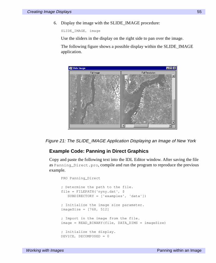
Creating Image Displays 55
imgdispl.fm Page 55 Wednesday, March 6, 2002 5:29 PM
6. Display the image with the SLIDE_IMAGE procedure:
SLIDE_IMAGE, image
Use the sliders in the display on the right side to pan over the image.
The following figure shows a possible display within the SLIDE_IMAGEapplication.
Example Code: Panning in Direct Graphics
Copy and paste the following text into the IDL Editor window. After saving the fileas Panning_Direct.pro, compile and run the program to reproduce the previousexample.
PRO Panning_Direct
; Determine the path to the file.file = FILEPATH('nyny.dat', $
SUBDIRECTORY = ['examples', 'data'])
; Initialize the image size parameter.imageSize = [768, 512]
; Import in the image from the file.image = READ_BINARY(file, DATA_DIMS = imageSize)
; Initialize the display.DEVICE, DECOMPOSED = 0
Figure 21: The SLIDE_IMAGE Application Displaying an Image of New York
Working with Images Panning within an Image
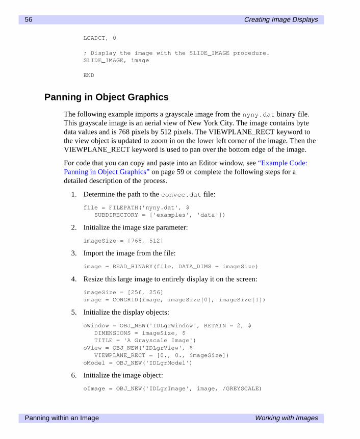
56 Creating Image Displays
imgdispl.fm Page 56 Wednesday, March 6, 2002 5:29 PM
LOADCT, 0
; Display the image with the SLIDE_IMAGE procedure.SLIDE_IMAGE, image
END
Panning in Object Graphics
The following example imports a grayscale image from the nyny.dat binary file.This grayscale image is an aerial view of New York City. The image contains bytedata values and is 768 pixels by 512 pixels. The VIEWPLANE_RECT keyword tothe view object is updated to zoom in on the lower left corner of the image. Then theVIEWPLANE_RECT keyword is used to pan over the bottom edge of the image.
For code that you can copy and paste into an Editor window, see “Example Code:Panning in Object Graphics” on page 59 or complete the following steps for adetailed description of the process.
1. Determine the path to the convec.dat file:
file = FILEPATH('nyny.dat', $SUBDIRECTORY = ['examples', 'data'])
2. Initialize the image size parameter:
imageSize = [768, 512]
3. Import the image from the file:
image = READ_BINARY(file, DATA_DIMS = imageSize)
4. Resize this large image to entirely display it on the screen:
imageSize = [256, 256]image = CONGRID(image, imageSize[0], imageSize[1])
5. Initialize the display objects:
oWindow = OBJ_NEW('IDLgrWindow', RETAIN = 2, $DIMENSIONS = imageSize, $TITLE = 'A Grayscale Image')
oView = OBJ_NEW('IDLgrView', $VIEWPLANE_RECT = [0., 0., imageSize])
oModel = OBJ_NEW('IDLgrModel')
6. Initialize the image object:
oImage = OBJ_NEW('IDLgrImage', image, /GREYSCALE)
Panning within an Image Working with Images
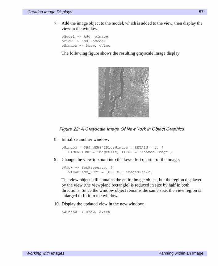
Creating Image Displays 57
imgdispl.fm Page 57 Wednesday, March 6, 2002 5:29 PM
7. Add the image object to the model, which is added to the view, then display theview in the window:
oModel -> Add, oImageoView -> Add, oModeloWindow -> Draw, oView
The following figure shows the resulting grayscale image display.
8. Initialize another window:
oWindow = OBJ_NEW('IDLgrWindow', RETAIN = 2, $DIMENSIONS = imageSize, TITLE = 'Zoomed Image')
9. Change the view to zoom into the lower left quarter of the image:
oView -> SetProperty, $VIEWPLANE_RECT = [0., 0., imageSize/2]
The view object still contains the entire image object, but the region displayedby the view (the viewplane rectangle) is reduced in size by half in bothdirections. Since the window object remains the same size, the view region isenlarged to fit it to the window.
10. Display the updated view in the new window:
oWindow -> Draw, oView
Figure 22: A Grayscale Image Of New York in Object Graphics
Working with Images Panning within an Image
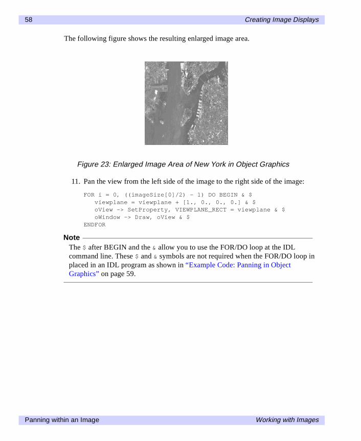
58 Creating Image Displays
imgdispl.fm Page 58 Wednesday, March 6, 2002 5:29 PM
The following figure shows the resulting enlarged image area.
11. Pan the view from the left side of the image to the right side of the image:
FOR i = 0, ((imageSize[0]/2) - 1) DO BEGIN & $viewplane = viewplane + [1., 0., 0., 0.] & $oView -> SetProperty, VIEWPLANE_RECT = viewplane & $oWindow -> Draw, oView & $
ENDFOR
NoteThe $ after BEGIN and the & allow you to use the FOR/DO loop at the IDLcommand line. These $ and & symbols are not required when the FOR/DO loop inplaced in an IDL program as shown in “Example Code: Panning in ObjectGraphics” on page 59.
Figure 23: Enlarged Image Area of New York in Object Graphics
Panning within an Image Working with Images
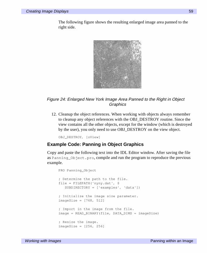
Creating Image Displays 59
imgdispl.fm Page 59 Wednesday, March 6, 2002 5:29 PM
The following figure shows the resulting enlarged image area panned to theright side.
12. Cleanup the object references. When working with objects always rememberto cleanup any object references with the OBJ_DESTROY routine. Since theview contains all the other objects, except for the window (which is destroyedby the user), you only need to use OBJ_DESTROY on the view object.
OBJ_DESTROY, [oView]
Example Code: Panning in Object Graphics
Copy and paste the following text into the IDL Editor window. After saving the fileas Panning_Object.pro, compile and run the program to reproduce the previousexample.
PRO Panning_Object
; Determine the path to the file.file = FILEPATH('nyny.dat', $
SUBDIRECTORY = ['examples', 'data'])
; Initialize the image size parameter.imageSize = [768, 512]
; Import in the image from the file.image = READ_BINARY(file, DATA_DIMS = imageSize)
; Resize the image.imageSize = [256, 256]
Figure 24: Enlarged New York Image Area Panned to the Right in ObjectGraphics
Working with Images Panning within an Image
60 Creating Image Displays
imgdispl.fm Page 60 Wednesday, March 6, 2002 5:29 PM
image = CONGRID(image, imageSize[0], imageSize[1])
; Initialize display objects.oWindow = OBJ_NEW('IDLgrWindow', RETAIN = 2, $
DIMENSIONS = imageSize, $TITLE = 'A Grayscale Image')
oView = OBJ_NEW('IDLgrView', $VIEWPLANE_RECT = [0., 0., imageSize])
oModel = OBJ_NEW('IDLgrModel')
; Initialize image object.oImage = OBJ_NEW('IDLgrImage', image, /GREYSCALE)
; Add the image object to the model, which is added to; the view, then display the view in the window.oModel -> Add, oImageoView -> Add, oModeloWindow -> Draw, oView
; Initialize another window.oWindow = OBJ_NEW('IDLgrWindow', RETAIN = 2, $
DIMENSIONS = imageSize, $TITLE = 'Panning Enlarged Image')
; Change view to zoom into the lower left quarter of; the image.viewplane = [0., 0., imageSize/2]oView -> SetProperty, VIEWPLANE_RECT = viewplane
; Display updated view in new window.oWindow -> Draw, oView
; Pan the view from the left side of the image to the; right side of the image.FOR i = 0, ((imageSize[0]/2) - 1) DO BEGIN
viewplane = viewplane + [1., 0., 0., 0.]oView -> SetProperty, VIEWPLANE_RECT = viewplaneoWindow -> Draw, oView
ENDFOR
; Cleanup object references.OBJ_DESTROY, [oView]
END
Panning within an Image Working with Images
Working with Color
This chapter describes the following topics:
Overview of Working with Color . . . . . . . . 62Loading Pre-defined Color Tables . . . . . . . 68
Modifying and Converting Color Tables . . 71Converting Between Image Types . . . . . . . 89
Highlighting Features with a Color Table . . 97Showing Variations in Uniform Areas . . . . 108
Applying Color Annotations to Images . . . 116
Working with Images 61
62 Working with Color
Overview of Working with Color
An overview of color systems, display devices, image types, and IDL’s interactionwith these elements provide a basis for understanding how to effectively extractinformation from your images.
Color Systems
Although numerous ways of specifying and measuring color exist, most colorsystems are three-dimensional in nature, relying on three values to define eachindividual color. Common color systems include RGB (red, green, and blue), HSV(hue, saturation, and value), HLS (hue, lightness, and saturation), and CMY (cyan,magenta, and yellow).
Computer display devices typically rely on the RGB color system. In IDL, the RGBcolor system is implemented with a three-dimensional coordinate system with thered, green, and blue dimensions ranging from 0 to 255 (the range of a byte data type).Each individual color definition consists of three numbers; a red value, a green value,and a blue value.
The following figure shows that each displayable color corresponds to a locationwithin a three-dimensional color cube. The origin, (0, 0, 0), where each colorcoordinate is 0, is black. The point at (255, 255, 255) is white and represents anadditive mixture of the full intensity of each of the three colors. Points along the maindiagonal—where the intensities of each of the three primary colors are equal—are
Overview of Working with Color Working with Images
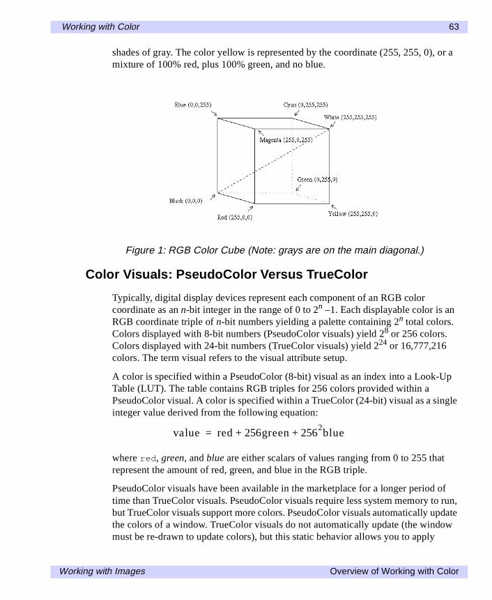
Working with Color 63
shades of gray. The color yellow is represented by the coordinate (255, 255, 0), or amixture of 100% red, plus 100% green, and no blue.
Color Visuals: PseudoColor Versus TrueColor
Typically, digital display devices represent each component of an RGB colorcoordinate as an n-bit integer in the range of 0 to 2n –1. Each displayable color is anRGB coordinate triple of n-bit numbers yielding a palette containing 2n total colors.Colors displayed with 8-bit numbers (PseudoColor visuals) yield 28 or 256 colors.Colors displayed with 24-bit numbers (TrueColor visuals) yield 224 or 16,777,216colors. The term visual refers to the visual attribute setup.
A color is specified within a PseudoColor (8-bit) visual as an index into a Look-UpTable (LUT). The table contains RGB triples for 256 colors provided within aPseudoColor visual. A color is specified within a TrueColor (24-bit) visual as a singleinteger value derived from the following equation:
where red, green, and blue are either scalars of values ranging from 0 to 255 thatrepresent the amount of red, green, and blue in the RGB triple.
PseudoColor visuals have been available in the marketplace for a longer period oftime than TrueColor visuals. PseudoColor visuals require less system memory to run,but TrueColor visuals support more colors. PseudoColor visuals automatically updatethe colors of a window. TrueColor visuals do not automatically update (the windowmust be re-drawn to update colors), but this static behavior allows you to apply
Figure 1: RGB Color Cube (Note: grays are on the main diagonal.)
value red 256green 2562blue+ +=
Working with Images Overview of Working with Color
64 Working with Color
different colors to different windows. With PseudoColor visuals, every IDL windowmust use the same colors.
The type of visual (PseudoColor or TrueColor) IDL uses by default depends more onyour computer system than IDL. On X Windows systems, IDL tries to set aTrueColor visual before a PseudoColor visual. If a TrueColor visual is not providedby the computer system, then IDL will set a PseudoColor visual. Also on X Windowssystems, the visual can be specified with the PSEUDO and TRUE keywords to theDEVICE command before the first window is opened within the IDL session. OnWindows and Macintosh systems, the type of visual depends upon the system setting.
NoteThis chapter assumes a TrueColor display is used. If a PseudoColor display willprovide a different behavior, this change in behavior will be noted.
How Colors are Associated with Indexed and RGB Images
Common images are either indexed or RGB (red, green, and blue). An indexed imageis a two-dimensional array of values ranging from 0 to 255. Indexed images areusually stored as byte data. A two-dimensional array of a different data type can bemade into an indexed image by scaling it to range from 0 to 255 with the BYTSCLfunction. See BYTSCL in the IDL Reference Guide for more information.
An indexed image does not explicitly contain any color information. Its pixel valuesrepresent indices into a color Look-Up Table (LUT). Colors are applied by usingthese indices to look up the corresponding RGB triple in the LUT. In some cases, thepixel values of an indexed image reflect the relative intensity of each pixel. In othercases, each pixel value is simply an index, in which case the image is usuallyintended to be associated with a specific LUT.
An RGB (red, green, and blue) image is a three-dimensional byte array, which doesmaintain its own color information. In an RGB image, each pixel is represented bythree values (a triple) to define its color. Computers commonly store scannedphotographs as RGB images. The color information is stored in three sections of athird dimension of the image. These sections are known as color channels, colorbands, or color layers. One channel represents the amount of red in the image (the redchannel), one channel represents the amount of green in the image (the greenchannel), and one channel represents the amount of blue in the images (the bluechannel).
Overview of Working with Color Working with Images
Working with Color 65
Color interleaving is a term used to describe which of the dimensions of an RGBimage contain the three color channel values. Three types of color interleaving aresupported by IDL:
• Pixel interleaving - the color information is contained in the first dimension,(3, n, m).
• Line interleaving - the color information is contained in the second dimension,(n, 3, m).
• Image interleaving - the color information is contained in the third dimension,(n, m, 3).
For PseudoColor visuals and indexed images, the LUT (usually just known as a colortable or color palette) is used to associate the value of a pixel with a color triple.Given 8-bit pixels (found in many PseudoColor visuals), a color table containing28 = 256 elements is required. The color table element with an index of i specifies thecolor for pixels with a value of i. Since indexed images do not maintain their owncolor information, these images are usually associated with color tables to providecolor information. Some indexed images are even saved to image files with anassociated color table.
Within IDL, a color table is represented by either a 3 by 256 byte array or three bytevectors of 256 elements each. In other words, a color table contains 256 RGB triples.The first component (column) in the 3 by 256 array is the red values of each triple,the second component is the green values, and the third component is the blue values.This array or these vectors can be created or changed to provide different color tableswithin IDL. IDL provides 41 pre-defined color tables.
PseudoColor visuals are only associated with indexed images and color tables. Youcan display RGB images on PseudoColor visuals with IDL by using theCOLOR_QUAN function. This function creates a color table for displaying the RGBimage and then maps this image to the new palette. See “Converting RGB Images toIndexed Images” on page 93 and COLOR_QUAN in the IDL Reference Guide for moreinformation.
Color tables were derived for PseudoColor visuals. TrueColor visuals (by default) donot typically utilize color tables. You can use color tables on TrueColor visuals ofIDL by setting the DECOMPOSED keyword to the DEVICE routine to a value ofzero (DEVICE, DECOMPOSED = 0). IDL must be instructed (by the user) to applycolor tables on TrueColor visuals. If you do not want a color table applied to awindow within a TrueColor visuals (when displaying an RGB image for example),set the DECOMPOSED keyword to one (DEVICE, DECOMPOSED = 1). You can use
Working with Images Overview of Working with Color
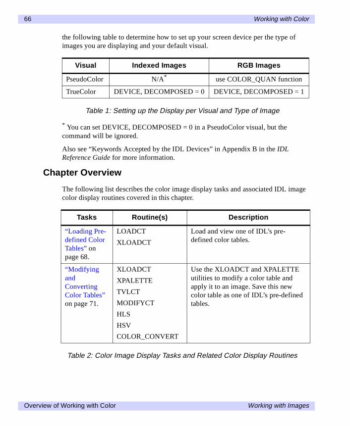
66 Working with Color
the following table to determine how to set up your screen device per the type ofimages you are displaying and your default visual.
* You can set DEVICE, DECOMPOSED = 0 in a PseudoColor visual, but thecommand will be ignored.
Also see “Keywords Accepted by the IDL Devices” in Appendix B in the IDLReference Guide for more information.
Chapter Overview
The following list describes the color image display tasks and associated IDL imagecolor display routines covered in this chapter.
Visual Indexed Images RGB Images
PseudoColor N/A* use COLOR_QUAN function
TrueColor DEVICE, DECOMPOSED = 0 DEVICE, DECOMPOSED = 1
Table 1: Setting up the Display per Visual and Type of Image
Tasks Routine(s) Description
“Loading Pre-defined ColorTables” onpage 68.
LOADCT
XLOADCT
Load and view one of IDL’s pre-defined color tables.
“ModifyingandConvertingColor Tables”on page 71.
XLOADCT
XPALETTE
TVLCT
MODIFYCT
HLS
HSV
COLOR_CONVERT
Use the XLOADCT and XPALETTEutilities to modify a color table andapply it to an image. Save this newcolor table as one of IDL’s pre-definedtables.
Table 2: Color Image Display Tasks and Related Color Display Routines
Overview of Working with Color Working with Images
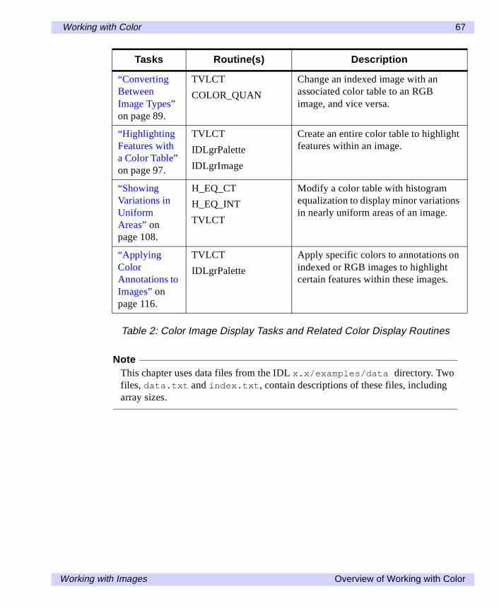
Working with Color 67
NoteThis chapter uses data files from the IDL x.x/examples/data directory. Twofiles, data.txt and index.txt, contain descriptions of these files, includingarray sizes.
“ConvertingBetweenImage Types”on page 89.
TVLCT
COLOR_QUAN
Change an indexed image with anassociated color table to an RGBimage, and vice versa.
“HighlightingFeatures witha Color Table”on page 97.
TVLCT
IDLgrPalette
IDLgrImage
Create an entire color table to highlightfeatures within an image.
“ShowingVariations inUniformAreas” onpage 108.
H_EQ_CT
H_EQ_INT
TVLCT
Modify a color table with histogramequalization to display minor variationsin nearly uniform areas of an image.
“ApplyingColorAnnotations toImages” onpage 116.
TVLCT
IDLgrPalette
Apply specific colors to annotations onindexed or RGB images to highlightcertain features within these images.
Tasks Routine(s) Description
Table 2: Color Image Display Tasks and Related Color Display Routines
Working with Images Overview of Working with Color
68 Working with Color
Loading Pre-defined Color Tables
Although you can define your own color tables, IDL provides 41 pre-defined colortables. You can access these tables through the LOADCT routine. Each color tablecontained within this routine is specified through an index value ranging from 0 to40.
TipIf you are running IDL on a TrueColor display, set DEVICE, DECOMPOSED = 0before your first color table related routine is used within an IDL session orprogram. See “How Colors are Associated with Indexed and RGB Images” onpage 64 for more information.
1. View a list of IDL’s tables and their related indices by calling LOADCTwithout an argument:
LOADCT
The following list is displayed in the Output Log:
% Compiled module: LOADCT.% Compiled module: FILEPATH.0-B-W LIMEAR 14-STEPS 28-Hardcandy1-BLUE/WHITE 15-STERN SPECIAL 29-Nature2-GRN-RED-BLU-WHT 16-Haze 30-Ocean3-RED TEMPERATURE 17-Blue-Pastel-Red 31-Peppermint4-BLU/GRN/RED/YEL 18-Pastels 32-Plasma5-STD GAMMA-II 19-Hue Sat Lightness 1 33-Blue-Red6-PRISM 20-Hue Sat Lightness 2 34-Rainbow7-RED-PURPLE 21-Hue Sat Value 1 35-Blue Waves8-GREEN/WHITE LINEAR 22-Hue Sat Value 2 36-Volcano9-GRN/WHT EXPOMENTIAL 23-Purple-Red+Stripes 37-Waves10-GREEN-PINK 24-Beach 38-Rainbow1811-BLUE_RED 25-Mac Style 39-Rainbow+white12-16 LEVEL 26-Eos A 40-Rainbow+black13-RAINBOW 27-Eos B
When running LOADCT without an argument, it will prompt you to enter thenumber of one of the above color tables at the IDL command line.
Loading Pre-defined Color Tables Working with Images
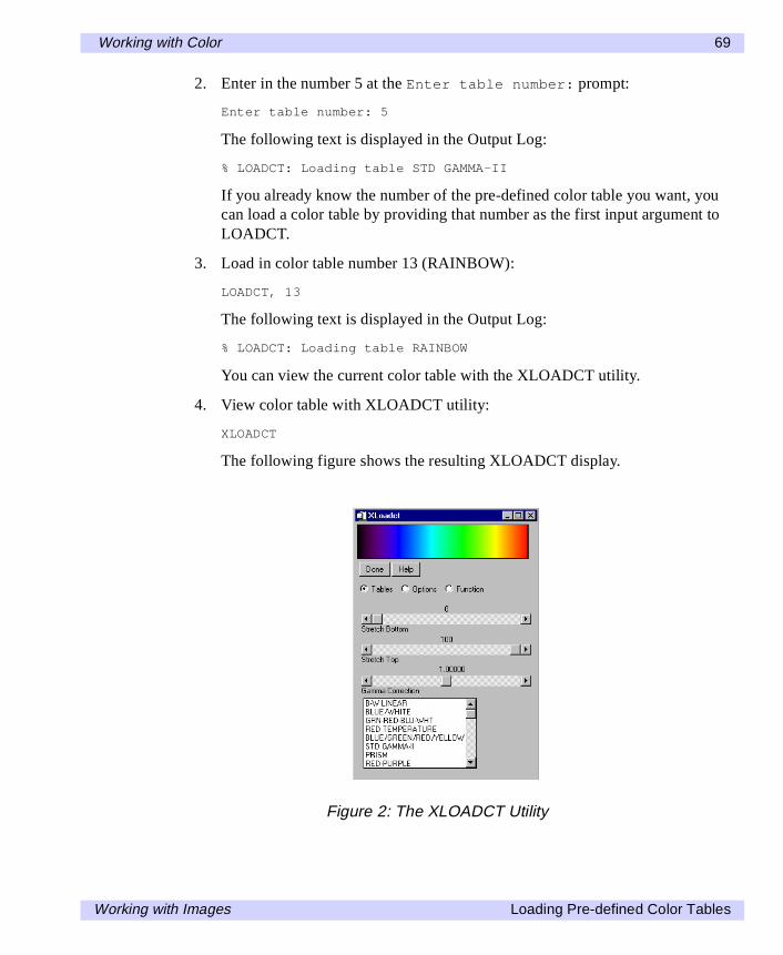
Working with Color 69
2. Enter in the number 5 at the Enter table number: prompt:
Enter table number: 5
The following text is displayed in the Output Log:
% LOADCT: Loading table STD GAMMA-II
If you already know the number of the pre-defined color table you want, youcan load a color table by providing that number as the first input argument toLOADCT.
3. Load in color table number 13 (RAINBOW):
LOADCT, 13
The following text is displayed in the Output Log:
% LOADCT: Loading table RAINBOW
You can view the current color table with the XLOADCT utility.
4. View color table with XLOADCT utility:
XLOADCT
The following figure shows the resulting XLOADCT display.
Figure 2: The XLOADCT Utility
Working with Images Loading Pre-defined Color Tables
70 Working with Color
This utility is designed to individually display each pre-defined color table.When the Done button is pressed, the selected color table automaticallybecomes IDL’s current color table. IDL maintains a color table onPseudoColor displays or when the DECOMPOSED keyword to the DEVICEcommand is set to zero (DEVICE, DECOMPOSED = 0) on TrueColor displays.XLOADCT also allows you to make adjustments to the current color table.Among other options, you can stretch the bottom, stretch the top, or apply agamma correction factor. See the next section, “Modifying and ConvertingColor Tables” on page 71, for more information.
Loading Pre-defined Color Tables Working with Images
Working with Color 71
Modifying and Converting Color Tables
IDL contains two graphical user interface (GUI) utilities for modifying a color table,XLOADCT and XPALETTE. “Using the XLOADCT Utility” (below) and “Usingthe XPALETTE Utility” on page 81 describe how to use these utilities to modifycolor tables. See “Highlighting Features with a Color Table” on page 97 for moreinformation on how to programmatically (without a GUI utility) modify and design acolor table. Then the “Using the MODIFYCT Routine” on page 87 section showshow to add the changed color table from XLOADCT and XPALETTE to IDL’s list ofpre-defined color tables.
The following examples are based on the default RGB (red, green, and blue) colorsystem. IDL also contains routines that allow you to use other color systemsincluding hue, saturation, and value (HSV) and hue, lightness, and saturation (HLS).These routines and color systems are explained in “Converting to Other ColorSystems” on page 88.
Using the XLOADCT Utility
The XLOADCT utility allows you to load one of IDL’s 41 pre-defined color tablesand change that color table if necessary. The following example shows how to useXLOADCT to load a color table and then change that table to highlight specificfeatures of an image. The indexed image used in this example is a computerizedtomography (CT) scan of a human thoracic cavity and is contained (without a defaultcolor table) within the ctscan.dat file in IDL’s examples/data directory.
For code that you can copy and paste into an IDL Editor window, see “ExampleCode: Using the XLOADCT Utility” on page 79 or complete the following steps fora detailed description of the process.
1. Determine the path to the ctscan.dat binary file:
ctscanFile = FILEPATH('ctscan.dat', $SUBDIRECTORY = ['examples', 'data'])
2. Initialize the image size parameter:
ctscanSize = [256, 256]
3. Import in the image from the file:
ctscanImage = READ_BINARY(ctscanFile, $DATA_DIMS = ctscanSize)
Working with Images Modifying and Converting Color Tables
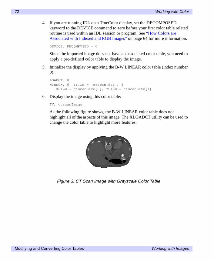
72 Working with Color
4. If you are running IDL on a TrueColor display, set the DECOMPOSEDkeyword to the DEVICE command to zero before your first color table relatedroutine is used within an IDL session or program. See “How Colors areAssociated with Indexed and RGB Images” on page 64 for more information.
DEVICE, DECOMPOSED = 0
Since the imported image does not have an associated color table, you need toapply a pre-defined color table to display the image.
5. Initialize the display by applying the B-W LINEAR color table (index number0):
LOADCT, 0WINDOW, 0, TITLE = 'ctscan.dat', $
XSIZE = ctscanSize[0], YSIZE = ctscanSize[1]
6. Display the image using this color table:
TV, ctscanImage
As the following figure shows, the B-W LINEAR color table does nothighlight all of the aspects of this image. The XLOADCT utility can be used tochange the color table to highlight more features.
Figure 3: CT Scan Image with Grayscale Color Table
Modifying and Converting Color Tables Working with Images
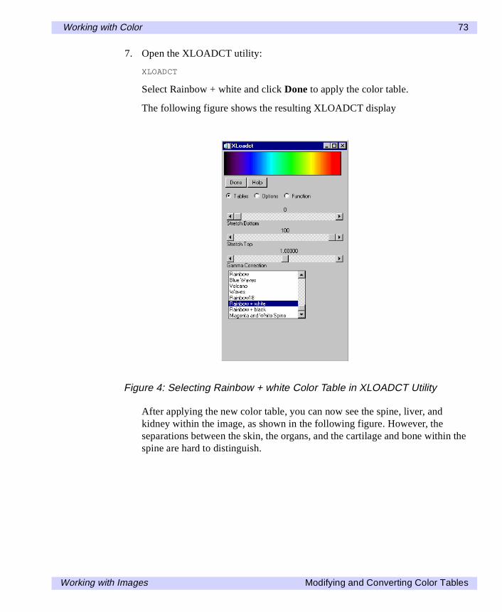
Working with Color 73
7. Open the XLOADCT utility:
XLOADCT
Select Rainbow + white and click Done to apply the color table.
The following figure shows the resulting XLOADCT display
After applying the new color table, you can now see the spine, liver, andkidney within the image, as shown in the following figure. However, theseparations between the skin, the organs, and the cartilage and bone within thespine are hard to distinguish.
Figure 4: Selecting Rainbow + white Color Table in XLOADCT Utility
Working with Images Modifying and Converting Color Tables
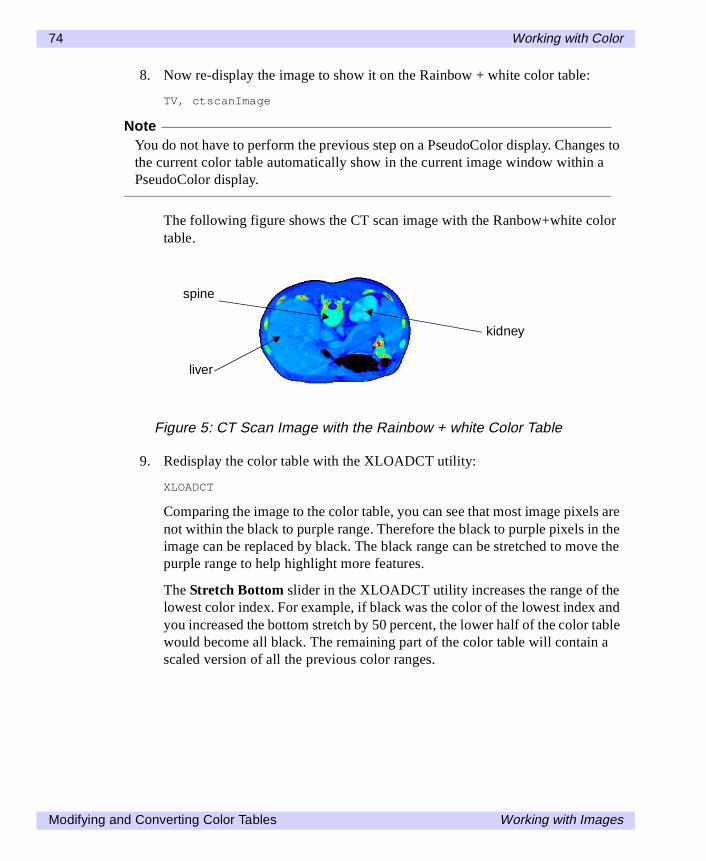
74 Working with Color
8. Now re-display the image to show it on the Rainbow + white color table:
TV, ctscanImage
NoteYou do not have to perform the previous step on a PseudoColor display. Changes tothe current color table automatically show in the current image window within aPseudoColor display.
The following figure shows the CT scan image with the Ranbow+white colortable.
9. Redisplay the color table with the XLOADCT utility:
XLOADCT
Comparing the image to the color table, you can see that most image pixels arenot within the black to purple range. Therefore the black to purple pixels in theimage can be replaced by black. The black range can be stretched to move thepurple range to help highlight more features.
The Stretch Bottom slider in the XLOADCT utility increases the range of thelowest color index. For example, if black was the color of the lowest index andyou increased the bottom stretch by 50 percent, the lower half of the color tablewould become all black. The remaining part of the color table will contain ascaled version of all the previous color ranges.
Figure 5: CT Scan Image with the Rainbow + white Color Table
spine
liver
kidney
Modifying and Converting Color Tables Working with Images
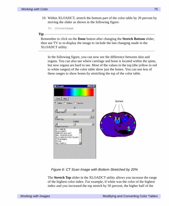
Working with Color 75
10. Within XLOADCT, stretch the bottom part of the color table by 20 percent bymoving the slider as shown in the following figure:
TV, ctscanImage
TipRemember to click on the Done button after changing the Stretch Bottom slider,then use TV to re-display the image to include the last changing made in theXLOADCT utility.
In the following figure, you can now see the difference between skin andorgans. You can also see where cartilage and bone is located within the spine,but now organs are hard to see. Most of the values in the top (the yellow to redto white ranges) of the color table show just the bones. You can use less ofthese ranges to show bones by stretching the top of the color table.
The Stretch Top slider in the XLOADCT utility allows you increase the rangeof the highest color index. For example, if white was the color of the highestindex and you increased the top stretch by 50 percent, the higher half of the
Figure 6: CT Scan Image with Bottom Stretched by 20%
bones
Working with Images Modifying and Converting Color Tables
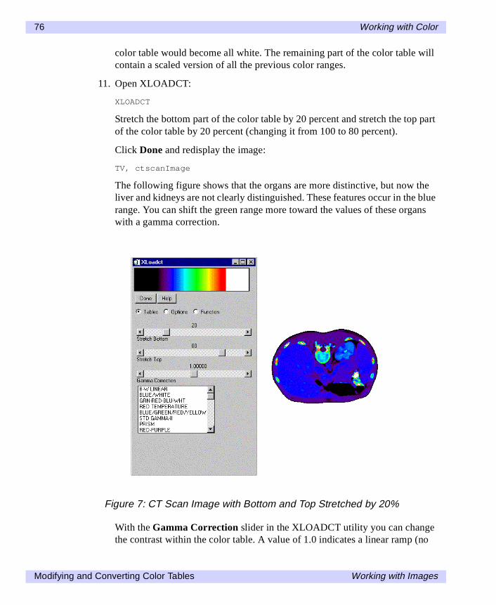
76 Working with Color
color table would become all white. The remaining part of the color table willcontain a scaled version of all the previous color ranges.
11. Open XLOADCT:
XLOADCT
Stretch the bottom part of the color table by 20 percent and stretch the top partof the color table by 20 percent (changing it from 100 to 80 percent).
Click Done and redisplay the image:
TV, ctscanImage
The following figure shows that the organs are more distinctive, but now theliver and kidneys are not clearly distinguished. These features occur in the bluerange. You can shift the green range more toward the values of these organswith a gamma correction.
With the Gamma Correction slider in the XLOADCT utility you can changethe contrast within the color table. A value of 1.0 indicates a linear ramp (no
Figure 7: CT Scan Image with Bottom and Top Stretched by 20%
Modifying and Converting Color Tables Working with Images
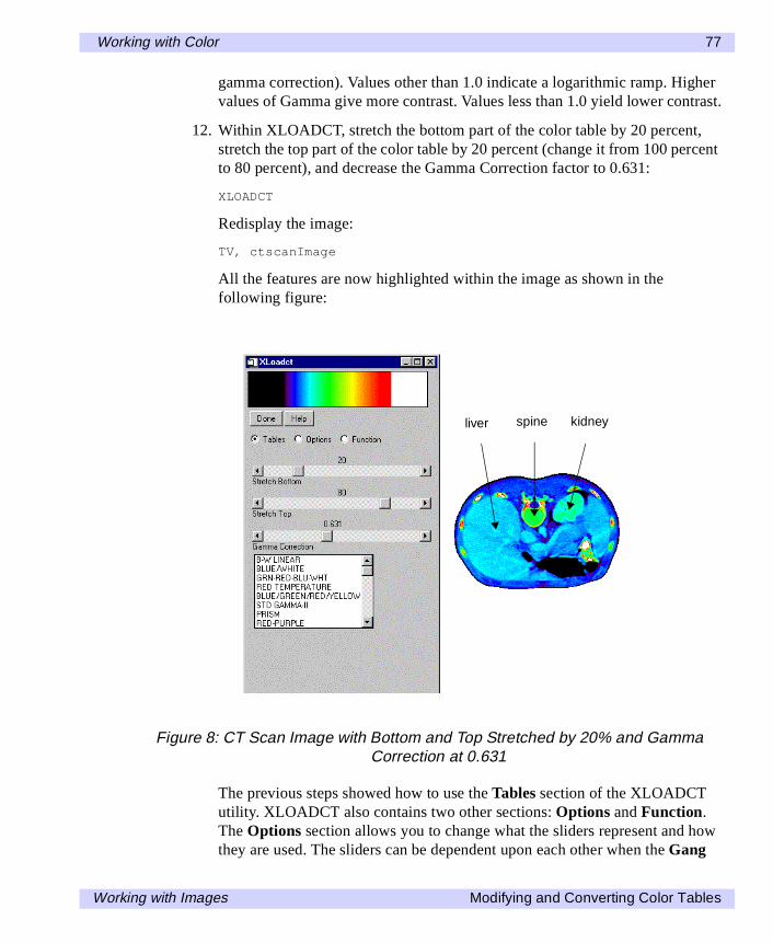
Working with Color 77
gamma correction). Values other than 1.0 indicate a logarithmic ramp. Highervalues of Gamma give more contrast. Values less than 1.0 yield lower contrast.
12. Within XLOADCT, stretch the bottom part of the color table by 20 percent,stretch the top part of the color table by 20 percent (change it from 100 percentto 80 percent), and decrease the Gamma Correction factor to 0.631:
XLOADCT
Redisplay the image:
TV, ctscanImage
All the features are now highlighted within the image as shown in thefollowing figure:
The previous steps showed how to use the Tables section of the XLOADCTutility. XLOADCT also contains two other sections: Options and Function.The Options section allows you to change what the sliders represent and howthey are used. The sliders can be dependent upon each other when the Gang
Figure 8: CT Scan Image with Bottom and Top Stretched by 20% and GammaCorrection at 0.631
liver spine kidney
Working with Images Modifying and Converting Color Tables
78 Working with Color
option is selected. When either the Stretch Bottom or Stretch Top sliders aremoved, the other ones reset to their default values (0 or 100, respectively). Thetop of the color table can be chopped off (the range of the Stretch Top is nowblack instead of the color at the original highest index) with the Chop option.The slider can also be changed to control intensity instead of index locationwith the Intensity option. The Stretch Bottom slider will darken the colortable and the Stretch Top slider will brighten the color table.
The Function section allows you to place control points which you can use tochange the color table with respect to the other colors in that table. The colortable function is shown as a straight line increasing from the lowest index (0)to the highest index (255). The x-axis ranges from 0 to 255 and the y-axisranges from 0 to 255. Moving a control point in the x-direction has the sameeffects as the previous sliders. Moving a control point in the y-directionchanges the color of that index to another color within the color table. Forexample, if a control point is red at an index of 128 and the color table is greenat an index of 92, when the control point is moved in the y-direction to anindex of 92, the color at that x-location will become green. To understand howthe Function section work, you can use it to highlight just the bones with theCT scan image.
13. Open XLOADCT:
XLOADCT
Select the Rainbow + white color table.
Switch to the Function section by selecting that option.
Select the Add Control Point button, and drag this new center control pointone half of the way to the right and one quarter of the way down as shown inthe following figure.
Click Done and redisplay the image:
TV, ctscanImage
Modifying and Converting Color Tables Working with Images
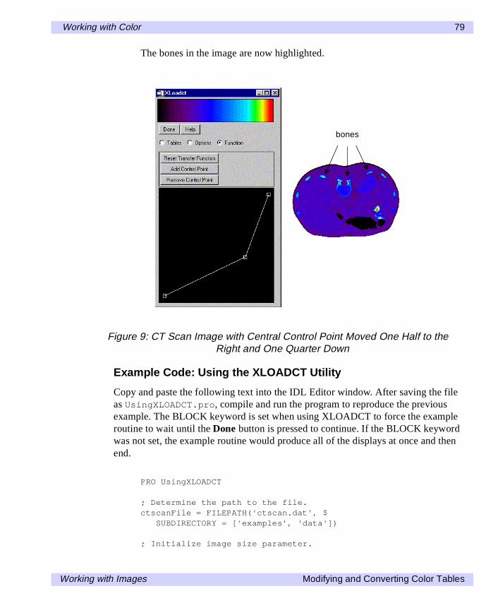
Working with Color 79
The bones in the image are now highlighted.
Example Code: Using the XLOADCT Utility
Copy and paste the following text into the IDL Editor window. After saving the fileas UsingXLOADCT.pro, compile and run the program to reproduce the previousexample. The BLOCK keyword is set when using XLOADCT to force the exampleroutine to wait until the Done button is pressed to continue. If the BLOCK keywordwas not set, the example routine would produce all of the displays at once and thenend.
PRO UsingXLOADCT
; Determine the path to the file.ctscanFile = FILEPATH('ctscan.dat', $
SUBDIRECTORY = ['examples', 'data'])
; Initialize image size parameter.
Figure 9: CT Scan Image with Central Control Point Moved One Half to theRight and One Quarter Down
bones
Working with Images Modifying and Converting Color Tables
80 Working with Color
ctscanSize = [256, 256]
; Import in the image from the file.ctscanImage = READ_BINARY(ctscanFile, $
DATA_DIMS = ctscanSize)
; Initialize display.DEVICE, DECOMPOSED = 0LOADCT, 0WINDOW, 0, TITLE = 'ctscan.dat', $
XSIZE = ctscanSize[0], YSIZE = ctscanSize[1]
; Display image.TV, ctscanImage
; Select and display the "Rainbow + white" color; tableXLOADCT, /BLOCKTV, ctscanImage
; Increase "Stretch Bottom" by 20%.XLOADCT, /BLOCKTV, ctscanImage
; Increase "Stretch Bottom" by 20% and decrease; "Stretch Top" by 20% (to 80%).XLOADCT, /BLOCKTV, ctscanImage
; Increase "Stretch Bottom" by 20%, decrease "Stretch; Top" by 20% (to 80%), and decrease "Gamma Correction"; to 0.631.XLOADCT, /BLOCKTV, ctscanImage
; Switch to "Function" section, select "Add Control; Point" and drag this center control point one quarter; of the way up and one quarter of the way left.XLOADCT, /BLOCKTV, ctscanImage
END
Modifying and Converting Color Tables Working with Images
Working with Color 81
Using the XPALETTE Utility
Another utility, XPALETTE, can be used to change a specific color table entry orrange of entries. This example uses a single color (orange) to highlight pixels withinthe spine of the CT scan image. Then, starting with the entry that was changed toorange, a range of entries is selected and replaced with a ramp from orange to whiteto highlight the bones within this image.
For code that you can copy and paste into an IDL Editor window, see “ExampleCode: Using the XPALETTE Utility” on page 85 or complete the following steps fora detailed description of the process.
1. Determine the path to the ctscan.dat binary file:
ctscanFile = FILEPATH('ctscan.dat', $SUBDIRECTORY = ['examples', 'data'])
2. Initialize the image size parameter:
ctscanSize = [256, 256]
3. Import in the image from the file:
ctscanImage = READ_BINARY(ctscanFile, $DATA_DIMS = ctscanSize)
4. If you are running IDL on a TrueColor display, set the DECOMPOSEDkeyword to the DEVICE command to zero before your first color table relatedroutine is used within an IDL session or program. See “How Colors areAssociated with Indexed and RGB Images” on page 64 for more information.
DEVICE, DECOMPOSED = 0
5. Display the image from the ctscan.dat file with the B-W LINEAR colortable:
LOADCT, 0WINDOW, 0, TITLE = 'ctscan.dat', $
XSIZE = ctscanSize[0], YSIZE = ctscanSize[1]TV, ctscanImage
Working with Images Modifying and Converting Color Tables
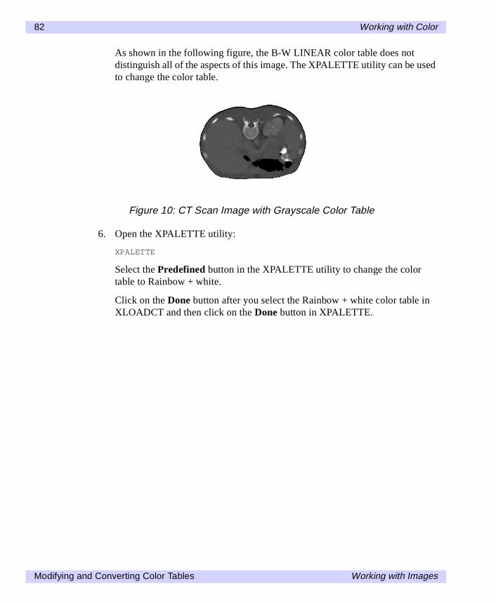
82 Working with Color
As shown in the following figure, the B-W LINEAR color table does notdistinguish all of the aspects of this image. The XPALETTE utility can be usedto change the color table.
6. Open the XPALETTE utility:
XPALETTE
Select the Predefined button in the XPALETTE utility to change the colortable to Rainbow + white.
Click on the Done button after you select the Rainbow + white color table inXLOADCT and then click on the Done button in XPALETTE.
Figure 10: CT Scan Image with Grayscale Color Table
Modifying and Converting Color Tables Working with Images
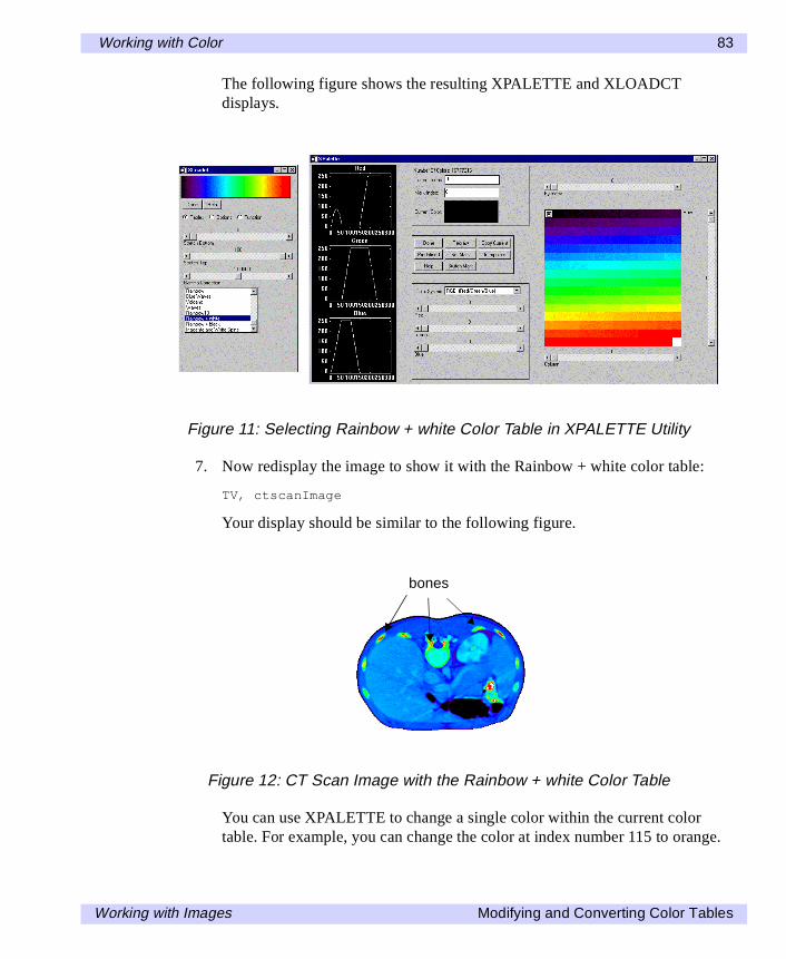
Working with Color 83
The following figure shows the resulting XPALETTE and XLOADCTdisplays.
7. Now redisplay the image to show it with the Rainbow + white color table:
TV, ctscanImage
Your display should be similar to the following figure.
You can use XPALETTE to change a single color within the current colortable. For example, you can change the color at index number 115 to orange.
Figure 11: Selecting Rainbow + white Color Table in XPALETTE Utility
Figure 12: CT Scan Image with the Rainbow + white Color Table
bones
Working with Images Modifying and Converting Color Tables
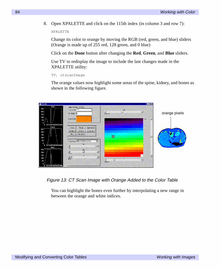
84 Working with Color
8. Open XPALETTE and click on the 115th index (in column 3 and row 7):
XPALETTE
Change its color to orange by moving the RGB (red, green, and blue) sliders(Orange is made up of 255 red, 128 green, and 0 blue)
Click on the Done button after changing the Red, Green, and Blue sliders.
Use TV to redisplay the image to include the last changes made in theXPALETTE utility:
TV, ctscanImage
The orange values now highlight some areas of the spine, kidney, and bones asshown in the following figure.
You can highlight the bones even further by interpolating a new range inbetween the orange and white indices.
Figure 13: CT Scan Image with Orange Added to the Color Table
orange pixels
Modifying and Converting Color Tables Working with Images
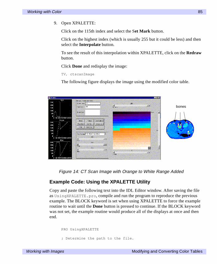
Working with Color 85
9. Open XPALETTE:
Click on the 115th index and select the Set Mark button.
Click on the highest index (which is usually 255 but it could be less) and thenselect the Interpolate button.
To see the result of this interpolation within XPALETTE, click on the Redrawbutton.
Click Done and redisplay the image:
TV, ctscanImage
The following figure displays the image using the modified color table.
Example Code: Using the XPALETTE Utility
Copy and paste the following text into the IDL Editor window. After saving the fileas UsingXPALETTE.pro, compile and run the program to reproduce the previousexample. The BLOCK keyword is set when using XPALETTE to force the exampleroutine to wait until the Done button is pressed to continue. If the BLOCK keywordwas not set, the example routine would produce all of the displays at once and thenend.
PRO UsingXPALETTE
; Determine the path to the file.
Figure 14: CT Scan Image with Orange to White Range Added
bones
Working with Images Modifying and Converting Color Tables
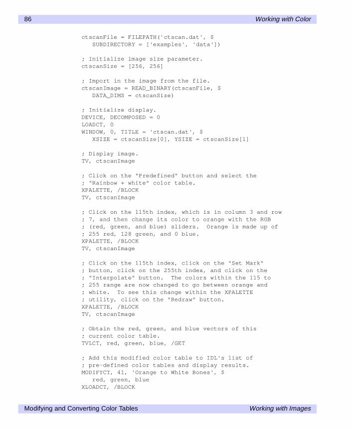
86 Working with Color
ctscanFile = FILEPATH('ctscan.dat', $SUBDIRECTORY = ['examples', 'data'])
; Initialize image size parameter.ctscanSize = [256, 256]
; Import in the image from the file.ctscanImage = READ_BINARY(ctscanFile, $
DATA_DIMS = ctscanSize)
; Initialize display.DEVICE, DECOMPOSED = 0LOADCT, 0WINDOW, 0, TITLE = 'ctscan.dat', $
XSIZE = ctscanSize[0], YSIZE = ctscanSize[1]
; Display image.TV, ctscanImage
; Click on the "Predefined" button and select the; "Rainbow + white" color table.XPALETTE, /BLOCKTV, ctscanImage
; Click on the 115th index, which is in column 3 and row; 7, and then change its color to orange with the RGB; (red, green, and blue) sliders. Orange is made up of; 255 red, 128 green, and 0 blue.XPALETTE, /BLOCKTV, ctscanImage
; Click on the 115th index, click on the "Set Mark"; button, click on the 255th index, and click on the; "Interpolate" button. The colors within the 115 to; 255 range are now changed to go between orange and; white. To see this change within the XPALETTE; utility, click on the "Redraw" button.XPALETTE, /BLOCKTV, ctscanImage
; Obtain the red, green, and blue vectors of this; current color table.TVLCT, red, green, blue, /GET
; Add this modified color table to IDL's list of; pre-defined color tables and display results.MODIFYCT, 41, 'Orange to White Bones', $
red, green, blueXLOADCT, /BLOCK
Modifying and Converting Color Tables Working with Images
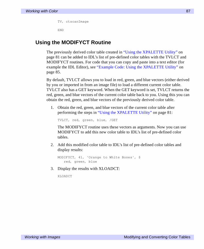
Working with Color 87
TV, ctscanImage
END
Using the MODIFYCT Routine
The previously derived color table created in “Using the XPALETTE Utility” onpage 81 can be added to IDL’s list of pre-defined color tables with the TVLCT andMODIFYCT routines. For code that you can copy and paste into a text editor (forexample the IDL Editor), see “Example Code: Using the XPALETTE Utility” onpage 85.
By default, TVLCT allows you to load in red, green, and blue vectors (either derivedby you or imported in from an image file) to load a different current color table.TVLCT also has a GET keyword. When the GET keyword is set, TVLCT returns thered, green, and blue vectors of the current color table back to you. Using this you canobtain the red, green, and blue vectors of the previously derived color table.
1. Obtain the red, green, and blue vectors of the current color table afterperforming the steps in “Using the XPALETTE Utility” on page 81:
TVLCT, red, green, blue, /GET
The MODIFYCT routine uses these vectors as arguments. Now you can useMODIFYCT to add this new color table to IDL’s list of pre-defined colortables.
2. Add this modified color table to IDL’s list of pre-defined color tables anddisplay results:
MODIFYCT, 41, 'Orange to White Bones', $red, green, blue
3. Display the results with XLOADCT:
XLOADCT
Working with Images Modifying and Converting Color Tables
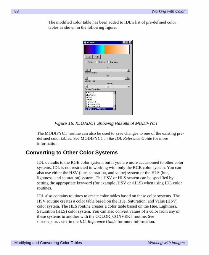
88 Working with Color
The modified color table has been added to IDL’s list of pre-defined colortables as shown in the following figure.
The MODIFYCT routine can also be used to save changes to one of the existing pre-defined color tables. See MODIFYCT in the IDL Reference Guide for moreinformation.
Converting to Other Color Systems
IDL defaults to the RGB color system, but if you are more accustomed to other colorsystems, IDL is not restricted to working with only the RGB color system. You canalso use either the HSV (hue, saturation, and value) system or the HLS (hue,lightness, and saturation) system. The HSV or HLS system can be specified bysetting the appropriate keyword (for example /HSV or /HLS) when using IDL colorroutines.
IDL also contains routines to create color tables based on these color systems. TheHSV routine creates a color table based on the Hue, Saturation, and Value (HSV)color system. The HLS routine creates a color table based on the Hue, Lightness,Saturation (HLS) color system. You can also convert values of a color from any ofthese systems to another with the COLOR_CONVERT routine. SeeCOLOR_CONVERT in the IDL Reference Guide for more information.
Figure 15: XLOADCT Showing Results of MODIFYCT
Modifying and Converting Color Tables Working with Images
Working with Color 89
Converting Between Image Types
Sometimes an image must be converted from indexed to RGB or RGB to indexed. Animage may be imported into IDL as an indexed image (from a PNG file for example)and you may need to export it as an RGB image (to a JPEG file for example). Ofcourse, the opposite may also occur: importing an RGB image and exporting it as anindexed image. See “How Colors are Associated with Indexed and RGB Images” onpage 64 for more information on indexed and RGB images.
Converting Indexed Images to RGB Images
The convec.dat file is a binary file containing an indexed image. The file containsan indexed image of the convection of the earth’s mantle. This file does not contain arelated color table. The following example applies a color table to this image and thenconverts the image and table to an RGB image (which contains its own colorinformation).
For code that you can copy and paste into an IDL Editor window, see “ExampleCode: Converting Indexed Images to RGB Images” on page 91 or complete thefollowing steps for a detailed description of the process.
1. Determine the path to the convec.dat binary file:
convecFile = FILEPATH('convec.dat', $SUBDIRECTORY = ['examples', 'data'])
2. Initialize the image size parameter:
convecSize = [248, 248]
3. Import in the image from the file:
convecImage = READ_BINARY(convecFile, $DATA_DIMS = convecSize)
4. If you are running IDL on a TrueColor display, set the DECOMPOSEDkeyword to the DEVICE command to zero before your first color table relatedroutine is used within an IDL session or program. See “How Colors areAssociated with Indexed and RGB Images” on page 64 for more information.
DEVICE, DECOMPOSED = 0
The EOS B color table is applied to highlight the features of this image.
Working with Images Converting Between Image Types
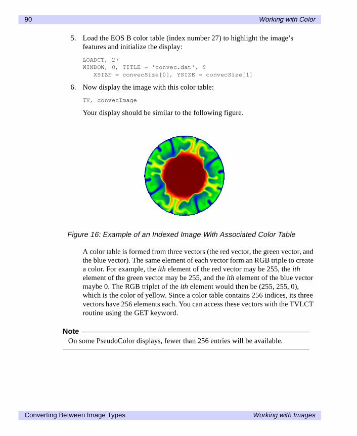
90 Working with Color
5. Load the EOS B color table (index number 27) to highlight the image’sfeatures and initialize the display:
LOADCT, 27WINDOW, 0, TITLE = 'convec.dat', $
XSIZE = convecSize[0], YSIZE = convecSize[1]
6. Now display the image with this color table:
TV, convecImage
Your display should be similar to the following figure.
A color table is formed from three vectors (the red vector, the green vector, andthe blue vector). The same element of each vector form an RGB triple to createa color. For example, the ith element of the red vector may be 255, the ithelement of the green vector may be 255, and the ith element of the blue vectormaybe 0. The RGB triplet of the ith element would then be (255, 255, 0),which is the color of yellow. Since a color table contains 256 indices, its threevectors have 256 elements each. You can access these vectors with the TVLCTroutine using the GET keyword.
NoteOn some PseudoColor displays, fewer than 256 entries will be available.
Figure 16: Example of an Indexed Image With Associated Color Table
Converting Between Image Types Working with Images
Working with Color 91
7. Access the values of the applied color table by setting the GET keyword to theTVLCT routine.
TVLCT, red, green, blue, /GET
This color table (color information) can be stored within the image byconverting it to an RGB image. For this example, the RGB image will be pixelinterleaved to be written to a JPEG file.
TipIf the original indexed image contains values of a data type other than byte, youshould byte-scale the image (with the BYTSCL routine) before using the followingmethod.
Before converting the indexed image into an RGB image, the resulting three-dimensional array must be initialized.
8. Initialize the data type and the dimensions of the resulting RGB image:
imageRGB = BYTARR(3, convecSize[0], convecSize[1])
Each channel of the resulting RGB image can be derived from the red, green,and blue vectors of the color table and the original indexed image.
9. Use the red, green, and blue vectors of the color table and the original indexedimage to form a single three-channelled image:
imageRGB[0, *, *] = red[convecImage]imageRGB[1, *, *] = green[convecImage]imageRGB[2, *, *] = blue[convecImage]
10. Write the resulting RGB image out to a JPEG file.
WRITE_JPEG, 'convecImage.jpg', imageRGB, TRUE = 1, $QUALITY = 100.
The TRUE keyword is set to 1 because the resulting RGB image is pixelinterleaved. See WRITE_JPEG for more information.
Example Code: Converting Indexed Images to RGB Images
Copy and paste the following text into the IDL Editor window. After saving the fileas IndexedToRGB.pro, compile and run the program to reproduce the previousexample.
PRO IndexedToRGB
Working with Images Converting Between Image Types
92 Working with Color
; Determine the path to the file.convecFile = FILEPATH('convec.dat', $
SUBDIRECTORY = ['examples', 'data'])
; Initialize the image size parameter.convecSize = [248, 248]
; Import in the image from the file.convecImage = READ_BINARY(convecFile, $
DATA_DIMS = convecSize)
; Initialize display.DEVICE, DECOMPOSED = 0LOADCT, 27WINDOW, 0, TITLE = 'convec.dat', $
XSIZE = convecSize[0], YSIZE = convecSize[1]
; Display image.TV, convecImage
; Obtain the red, green, and blue vectors that form the; current color table.TVLCT, red, green, blue, /GET
; Initialize the resulting RGB image.imageRGB = BYTARR(3, convecSize[0], convecSize[1])
; Derive each color image from the vectors of the; current color table.imageRGB[0, *, *] = red[convecImage]imageRGB[1, *, *] = green[convecImage]imageRGB[2, *, *] = blue[convecImage]
; Write the resulting RGB image out to a JPEG file.WRITE_JPEG, 'convec.jpg', imageRGB, TRUE = 1, $
QUALITY = 100.
END
Converting Between Image Types Working with Images
Working with Color 93
Converting RGB Images to Indexed Images
The elev_t.jpg file contains a pixel interleaved RGB image, which has its owncolor information. This example converts the image to an indexed image with anassociated color table.
For code that you can copy and paste into an IDL Editor window, see “ExampleCode: Converting RGB Images to Indexed Images” on page 95 or complete thefollowing steps for a detailed description of the process.
1. Determine the path to the elev_t.jpg file:
elev_tFile = FILEPATH('elev_t.jpg', $SUBDIRECTORY = ['examples', 'data'])
2. Import in the image from the elev_t.jpg file into IDL:
READ_JPEG, elev_tFile, elev_tImage
3. Determine the size of the imported image:
elev_tSize = SIZE(elev_tImage, /DIMENSIONS)
4. If you are running IDL on a TrueColor display, set the DECOMPOSEDkeyword to the DEVICE command to one before your first RGB image isdisplayed within an IDL session or program. See “How Colors are Associatedwith Indexed and RGB Images” on page 64 for more information:
DEVICE, DECOMPOSED = 1
5. Initialize the display:
WINDOW, 0, TITLE = 'elev_t.jpg', $XSIZE = elev_tSize[1], YSIZE = elev_tSize[2]
6. Display the imported image:
TV, elev_tImage, TRUE = 1
Working with Images Converting Between Image Types
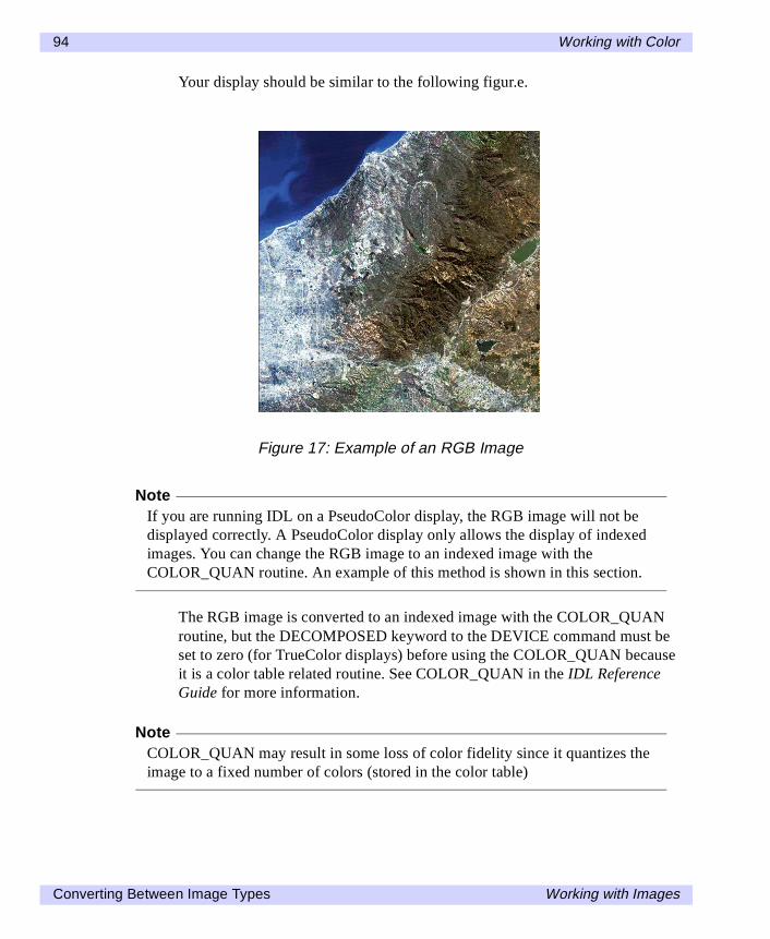
94 Working with Color
Your display should be similar to the following figur.e.
NoteIf you are running IDL on a PseudoColor display, the RGB image will not bedisplayed correctly. A PseudoColor display only allows the display of indexedimages. You can change the RGB image to an indexed image with theCOLOR_QUAN routine. An example of this method is shown in this section.
The RGB image is converted to an indexed image with the COLOR_QUANroutine, but the DECOMPOSED keyword to the DEVICE command must beset to zero (for TrueColor displays) before using the COLOR_QUAN becauseit is a color table related routine. See COLOR_QUAN in the IDL ReferenceGuide for more information.
NoteCOLOR_QUAN may result in some loss of color fidelity since it quantizes theimage to a fixed number of colors (stored in the color table)
Figure 17: Example of an RGB Image
Converting Between Image Types Working with Images
Working with Color 95
7. If you are running IDL on a TrueColor display, set the DECOMPOSEDkeyword to the DEVICE command to zero before your first color table relatedroutine is used within an IDL session or program. See “How Colors areAssociated with Indexed and RGB Images” on page 64 for more information.
DEVICE, DECOMPOSED = 0
8. Convert the RGB image to an indexed image with an associated color table:
imageIndexed = COLOR_QUAN(elev_tImage, 1, red, green, $blue)
9. Write the resulting indexed image and its associated color table out to a PNGfile:
WRITE_PNG, 'elev_t.png', imageIndexed, red, green, blue
Example Code: Converting RGB Images to Indexed Images
Copy and paste the following text into the IDL Editor window. After saving the fileas RGBToIndexed.pro, compile and run the program to reproduce the previousexample.
PRO RGBToIndexed
; Determine path to the "elev_t.jpg" file.elev_tFile = FILEPATH('elev_t.jpg', $
SUBDIRECTORY = ['examples', 'data'])
; Import image from file into IDL.READ_JPEG, elev_tFile, elev_tImage
; Determine the size of the imported image.elev_tSize = SIZE(elev_tImage, /DIMENSIONS)
; Initialize display.DEVICE, DECOMPOSED = 1WINDOW, 0, TITLE = 'elev_t.jpg', $
XSIZE = elev_tSize[1], YSIZE = elev_tSize[2]
; Display image.TV, elev_tImage, TRUE = 1
; Convert RGB image to indexed image with associated; color table.DEVICE, DECOMPOSED = 0imageIndexed = COLOR_QUAN(elev_tImage, 1, red, green, $
blue)
Working with Images Converting Between Image Types
96 Working with Color
; Write resulting image and its color table to a PNG; file.WRITE_PNG, 'elev_t.png', imageIndexed, red, green, blue
END
Converting Between Image Types Working with Images
Working with Color 97
Highlighting Features with a Color Table
For indexed images, entire color tables can be derived to highlight specific features.Color tables are usually designed to vary within certain ranges to show dramaticchanges within an image. Some color tables are designed to highlight features withdrastic color change in adjacent ranges (for example setting 0 through 20 to black andsetting 21 through 40 to white). Regardless, some features within an image may notbe significantly highlighted by IDL’s 41 pre-defined color tables.
NoteColor tables are associated with indexed images. RGB images already contain theirown color information. If you want to derive a color table for an RGB image, youshould convert it to an indexed image with the COLOR_QUAN routine. You shouldalso set COLOR_QUAN’s CUBE keyword to 6 to insure the resulting indexedimage is an intensity representation of the original RGB image. See COLOR_QUANin the IDL Reference Guide for more information
Highlighting Features with Color in Direct Graphics
The data in the mineral.png file in the examples/data directory comes with itsown color table. The following example will apply this related color table, then a pre-defined color table, and finally derive a new color table to highlight specific features.
For code that you can copy and paste into an IDL Editor window, see “ExampleCode: Highlighting Features with Color in Direct Graphics” on page 101 or completethe following steps for a detailed description of the process.
1. Determine the path to the mineral.png file:
mineralFile = FILEPATH(‘mineral.png', $SUBDIRECTORY = [‘examples', ‘data'])
2. Import the image from the minernal.png file into IDL:
mineralImage = READ_PNG(mineralFile, red, green, blue)
The image's associated color table is contained within the resulting red, green,and blue vectors.
3. Determine the size of the imported image:
mineralSize = SIZE(mineralImage, /DIMENSIONS)
Working with Images Highlighting Features with a Color Table
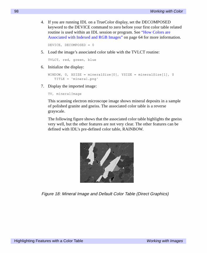
98 Working with Color
4. If you are running IDL on a TrueColor display, set the DECOMPOSEDkeyword to the DEVICE command to zero before your first color table relatedroutine is used within an IDL session or program. See “How Colors areAssociated with Indexed and RGB Images” on page 64 for more information.
DEVICE, DECOMPOSED = 0
5. Load the image’s associated color table with the TVLCT routine:
TVLCT, red, green, blue
6. Initialize the display:
WINDOW, 0, XSIZE = mineralSize[0], YSIZE = mineralSize[1], $TITLE = 'mineral.png'
7. Display the imported image:
TV, mineralImage
This scanning electron microscope image shows mineral deposits in a sampleof polished granite and gneiss. The associated color table is a reversegrayscale.
The following figure shows that the associated color table highlights the gneissvery well, but the other features are not very clear. The other features can bedefined with IDL’s pre-defined color table, RAINBOW.
Figure 18: Mineral Image and Default Color Table (Direct Graphics)
Highlighting Features with a Color Table Working with Images
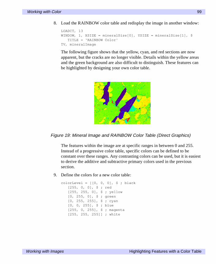
Working with Color 99
8. Load the RAINBOW color table and redisplay the image in another window:
LOADCT, 13WINDOW, 1, XSIZE = mineralSize[0], YSIZE = mineralSize[1], $
TITLE = ‘RAINBOW Color'TV, mineralImage
The following figure shows that the yellow, cyan, and red sections are nowapparent, but the cracks are no longer visible. Details within the yellow areasand the green background are also difficult to distinguish. These features canbe highlighted by designing your own color table.
The features within the image are at specific ranges in between 0 and 255.Instead of a progressive color table, specific colors can be defined to beconstant over these ranges. Any contrasting colors can be used, but it is easiestto derive the additive and subtractive primary colors used in the previoussection.
9. Define the colors for a new color table:
colorLevel = [[0, 0, 0], $ ; black[255, 0, 0], $ ; red[255, 255, 0], $ ; yellow[0, 255, 0], $ ; green[0, 255, 255], $ ; cyan[0, 0, 255], $ ; blue[255, 0, 255], $ ; magenta[255, 255, 255]] ; white
Figure 19: Mineral Image and RAINBOW Color Table (Direct Graphics)
Working with Images Highlighting Features with a Color Table
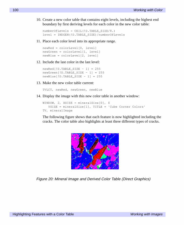
100 Working with Color
10. Create a new color table that contains eight levels, including the highest endboundary by first deriving levels for each color in the new color table:
numberOfLevels = CEIL(!D.TABLE_SIZE/8.)level = INDGEN(!D.TABLE_SIZE)/numberOfLevels
11. Place each color level into its appropriate range.
newRed = colorLevel[0, level]newGreen = colorLevel[1, level]newBlue = colorLevel[2, level]
12. Include the last color in the last level:
newRed[!D.TABLE_SIZE - 1] = 255newGreen[!D.TABLE_SIZE - 1] = 255newBlue[!D.TABLE_SIZE - 1] = 255
13. Make the new color table current:
TVLCT, newRed, newGreen, newBlue
14. Display the image with this new color table in another window:
WINDOW, 2, XSIZE = mineralSize[0], $YSIZE = mineralSize[1], TITLE = 'Cube Corner Colors'
TV, mineralImage
The following figure shows that each feature is now highlighted including thecracks. The color table also highlights at least three different types of cracks.
Figure 20: Mineral Image and Derived Color Table (Direct Graphics)
Highlighting Features with a Color Table Working with Images
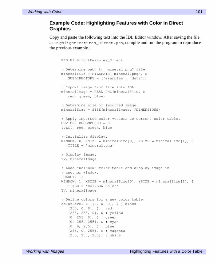
Working with Color 101
Example Code: Highlighting Features with Color in DirectGraphics
Copy and paste the following text into the IDL Editor window. After saving the fileas HighlightFeatures_Direct.pro, compile and run the program to reproducethe previous example.
PRO HighlightFeatures_Direct
; Determine path to "mineral.png" file.mineralFile = FILEPATH('mineral.png', $
SUBDIRECTORY = ['examples', 'data'])
; Import image from file into IDL.mineralImage = READ_PNG(mineralFile, $
red, green, blue)
; Determine size of imported image.mineralSize = SIZE(mineralImage, /DIMENSIONS)
; Apply imported color vectors to current color table.DEVICE, DECOMPOSED = 0TVLCT, red, green, blue
; Initialize display.WINDOW, 0, XSIZE = mineralSize[0], YSIZE = mineralSize[1], $
TITLE = 'mineral.png'
; Display image.TV, mineralImage
; Load "RAINBOW" color table and display image in; another window.LOADCT, 13WINDOW, 1, XSIZE = mineralSize[0], YSIZE = mineralSize[1], $
TITLE = 'RAINBOW Color'TV, mineralImage
; Define colors for a new color table.colorLevel = [[0, 0, 0], $ ; black
[255, 0, 0], $ ; red[255, 255, 0], $ ; yellow[0, 255, 0], $ ; green[0, 255, 255], $ ; cyan[0, 0, 255], $ ; blue[255, 0, 255], $ ; magenta[255, 255, 255]] ; white
Working with Images Highlighting Features with a Color Table
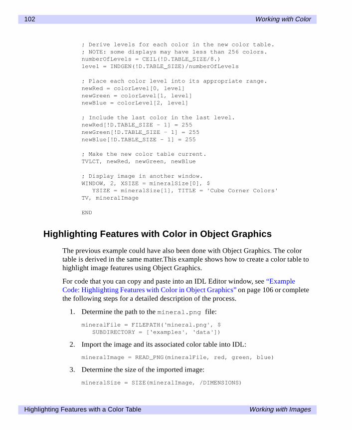
102 Working with Color
; Derive levels for each color in the new color table.; NOTE: some displays may have less than 256 colors.numberOfLevels = CEIL(!D.TABLE_SIZE/8.)level = INDGEN(!D.TABLE_SIZE)/numberOfLevels
; Place each color level into its appropriate range.newRed = colorLevel[0, level]newGreen = colorLevel[1, level]newBlue = colorLevel[2, level]
; Include the last color in the last level.newRed[!D.TABLE_SIZE - 1] = 255newGreen[!D.TABLE_SIZE - 1] = 255newBlue[!D.TABLE_SIZE - 1] = 255
; Make the new color table current.TVLCT, newRed, newGreen, newBlue
; Display image in another window.WINDOW, 2, XSIZE = mineralSize[0], $
YSIZE = mineralSize[1], TITLE = 'Cube Corner Colors'TV, mineralImage
END
Highlighting Features with Color in Object Graphics
The previous example could have also been done with Object Graphics. The colortable is derived in the same matter.This example shows how to create a color table tohighlight image features using Object Graphics.
For code that you can copy and paste into an IDL Editor window, see “ExampleCode: Highlighting Features with Color in Object Graphics” on page 106 or completethe following steps for a detailed description of the process.
1. Determine the path to the mineral.png file:
mineralFile = FILEPATH(‘mineral.png', $SUBDIRECTORY = [‘examples', ‘data'])
2. Import the image and its associated color table into IDL:
mineralImage = READ_PNG(mineralFile, red, green, blue)
3. Determine the size of the imported image:
mineralSize = SIZE(mineralImage, /DIMENSIONS)
Highlighting Features with a Color Table Working with Images
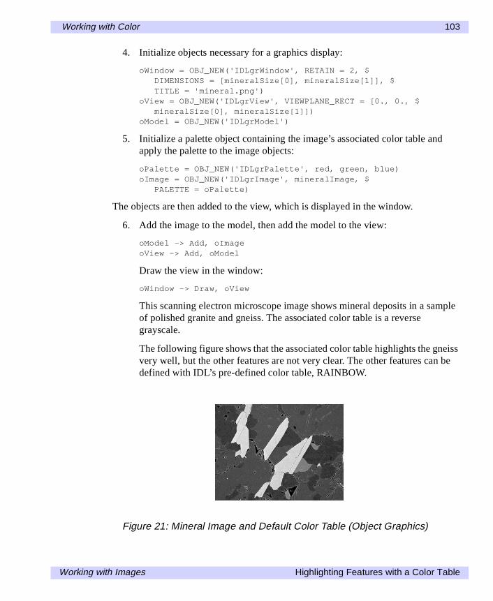
Working with Color 103
4. Initialize objects necessary for a graphics display:
oWindow = OBJ_NEW('IDLgrWindow', RETAIN = 2, $DIMENSIONS = [mineralSize[0], mineralSize[1]], $TITLE = 'mineral.png')
oView = OBJ_NEW('IDLgrView', VIEWPLANE_RECT = [0., 0., $mineralSize[0], mineralSize[1]])
oModel = OBJ_NEW('IDLgrModel')
5. Initialize a palette object containing the image’s associated color table andapply the palette to the image objects:
oPalette = OBJ_NEW('IDLgrPalette', red, green, blue)oImage = OBJ_NEW('IDLgrImage', mineralImage, $
PALETTE = oPalette)
The objects are then added to the view, which is displayed in the window.
6. Add the image to the model, then add the model to the view:
oModel -> Add, oImageoView -> Add, oModel
Draw the view in the window:
oWindow -> Draw, oView
This scanning electron microscope image shows mineral deposits in a sampleof polished granite and gneiss. The associated color table is a reversegrayscale.
The following figure shows that the associated color table highlights the gneissvery well, but the other features are not very clear. The other features can bedefined with IDL’s pre-defined color table, RAINBOW.
Figure 21: Mineral Image and Default Color Table (Object Graphics)
Working with Images Highlighting Features with a Color Table
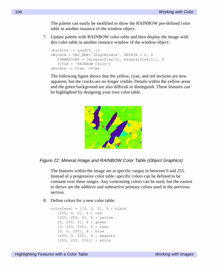
104 Working with Color
The palette can easily be modified to show the RAINBOW pre-defined colortable in another instance of the window object.
7. Update palette with RAINBOW color table and then display the image withthis color table in another instance window of the window object:
oPalette -> LoadCT, 13oWindow = OBJ_NEW('IDLgrWindow', RETAIN = 2, $
DIMENSIONS = [mineralSize[0], mineralSize[1]], $TITLE = 'RAINBOW Color')
oWindow -> Draw, oView
The following figure shows that the yellow, cyan, and red sections are nowapparent, but the cracks are no longer visible. Details within the yellow areasand the green background are also difficult to distinguish. These features canbe highlighted by designing your own color table.
The features within the image are at specific ranges in between 0 and 255.Instead of a progressive color table, specific colors can be defined to beconstant over these ranges. Any contrasting colors can be used, but the easiestto derive are the additive and subtractive primary colors used in the previoussection.
8. Define colors for a new color table:
colorLevel = [[0, 0, 0], $ ; black[255, 0, 0], $ ; red[255, 255, 0], $ ; yellow[0, 255, 0], $ ; green[0, 255, 255], $ ; cyan[0, 0, 255], $ ; blue[255, 0, 255], $ ; magenta[255, 255, 255]] ; white
Figure 22: Mineral Image and RAINBOW Color Table (Object Graphics)
Highlighting Features with a Color Table Working with Images
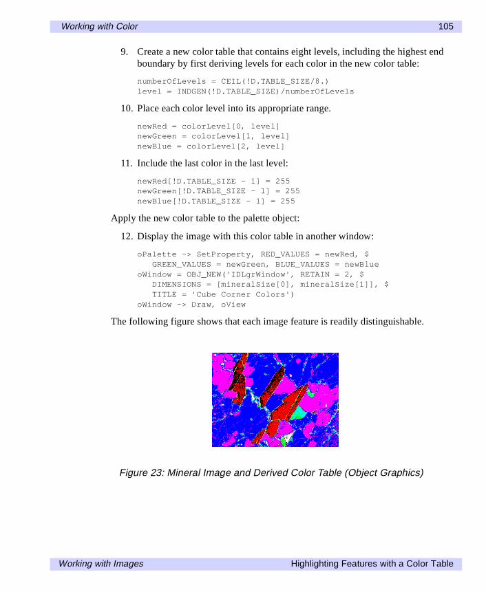
Working with Color 105
9. Create a new color table that contains eight levels, including the highest endboundary by first deriving levels for each color in the new color table:
numberOfLevels = CEIL(!D.TABLE_SIZE/8.)level = INDGEN(!D.TABLE_SIZE)/numberOfLevels
10. Place each color level into its appropriate range.
newRed = colorLevel[0, level]newGreen = colorLevel[1, level]newBlue = colorLevel[2, level]
11. Include the last color in the last level:
newRed[!D.TABLE_SIZE - 1] = 255newGreen[!D.TABLE_SIZE - 1] = 255newBlue[!D.TABLE_SIZE - 1] = 255
Apply the new color table to the palette object:
12. Display the image with this color table in another window:
oPalette -> SetProperty, RED_VALUES = newRed, $GREEN_VALUES = newGreen, BLUE_VALUES = newBlue
oWindow = OBJ_NEW('IDLgrWindow', RETAIN = 2, $DIMENSIONS = [mineralSize[0], mineralSize[1]], $TITLE = 'Cube Corner Colors')
oWindow -> Draw, oView
The following figure shows that each image feature is readily distinguishable.
Figure 23: Mineral Image and Derived Color Table (Object Graphics)
Working with Images Highlighting Features with a Color Table
106 Working with Color
13. Clean-up object references. When working with objects always remember toclean-up any object references with the OBJ_DESTROY routine. Since theview contains all the other objects, except for the window (which is destroyedby the user), you only need to use OBJ_DESTROY on the view and the paletteobject:
OBJ_DESTROY, [oView, oPalette]
Example Code: Highlighting Features with Color in ObjectGraphics
Copy and paste the following text into the IDL Editor window. After saving the fileas HighlightFeatures_Object.pro, compile and run the program to reproducethe previous example.
PRO HighlightFeatures_Object
; Determine path to "mineral.png" file.mineralFile = FILEPATH('mineral.png', $
SUBDIRECTORY = ['examples', 'data'])
; Import image from file into IDL.mineralImage = READ_PNG(mineralFile, $
red, green, blue)
; Determine size of imported image.mineralSize = SIZE(mineralImage, /DIMENSIONS)
; Initialize objects.; Initialize display.oWindow = OBJ_NEW('IDLgrWindow', RETAIN = 2, $
DIMENSIONS = [mineralSize[0], mineralSize[1]], $TITLE = 'mineral.png')
oView = OBJ_NEW('IDLgrView', VIEWPLANE_RECT = [0., 0., $mineralSize[0], mineralSize[1]])
oModel = OBJ_NEW('IDLgrModel'); Initialize palette and image.oPalette = OBJ_NEW('IDLgrPalette', red, green, blue)oImage = OBJ_NEW('IDLgrImage', mineralImage, $
PALETTE = oPalette)
; Add image to model, then model to view, and draw final; view in window.oModel -> Add, oImageoView -> Add, oModeloWindow -> Draw, oView
Highlighting Features with a Color Table Working with Images
Working with Color 107
; Update palette with RAINBOW color table and then; display image in another instance of the window object.oPalette -> LoadCT, 13oWindow = OBJ_NEW('IDLgrWindow', RETAIN = 2, $
DIMENSIONS = [mineralSize[0], mineralSize[1]], $TITLE = 'RAINBOW Color')
oWindow -> Draw, oView
; Define colors for a new color table.colorLevel = [[0, 0, 0], $ ; black
[255, 0, 0], $ ; red[255, 255, 0], $ ; yellow[0, 255, 0], $ ; green[0, 255, 255], $ ; cyan[0, 0, 255], $ ; blue[255, 0, 255], $ ; magenta[255, 255, 255]] ; white
; Derive levels for each color in the new color table.; NOTE: some displays may have less than 256 colors.numberOfLevels = CEIL(!D.TABLE_SIZE/8.)level = INDGEN(!D.TABLE_SIZE)/numberOfLevels
; Place each color level into its appropriate range.newRed = colorLevel[0, level]newGreen = colorLevel[1, level]newBlue = colorLevel[2, level]
; Include the last color in the last level.newRed[!D.TABLE_SIZE - 1] = 255newGreen[!D.TABLE_SIZE - 1] = 255newBlue[!D.TABLE_SIZE - 1] = 255
; Update palette with new color table and then; display image in another instance of the window object.oPalette -> SetProperty, RED_VALUES = newRed, $
GREEN_VALUES = newGreen, BLUE_VALUES = newBlueoWindow = OBJ_NEW('IDLgrWindow', RETAIN = 2, $
DIMENSIONS = [mineralSize[0], mineralSize[1]], $TITLE = 'Cube Corner Colors')
oWindow -> Draw, oView
; Clean-up object references.OBJ_DESTROY, [oView, oPalette]
END
Working with Images Highlighting Features with a Color Table
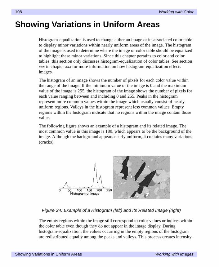
108 Working with Color
Showing Variations in Uniform Areas
Histogram-equalization is used to change either an image or its associated color tableto display minor variations within nearly uniform areas of the image. The histogramof the image is used to determine where the image or color table should be equalizedto highlight these minor variations. Since this chapter pertains to color and colortables, this section only discusses histogram-equalization of color tables. See sectionxxx in chapter xxx for more information on how histogram-equalization effectsimages.
The histogram of an image shows the number of pixels for each color value withinthe range of the image. If the minimum value of the image is 0 and the maximumvalue of the image is 255, the histogram of the image shows the number of pixels foreach value ranging between and including 0 and 255. Peaks in the histogramrepresent more common values within the image which usually consist of nearlyuniform regions. Valleys in the histogram represent less common values. Emptyregions within the histogram indicate that no regions within the image contain thosevalues.
The following figure shows an example of a histogram and its related image. Themost common value in this image is 180, which appears to be the background of theimage. Although the background appears nearly uniform, it contains many variations(cracks).
The empty regions within the image still correspond to color values or indices withinthe color table even though they do not appear in the image display. Duringhistogram-equalization, the values occurring in the empty regions of the histogramare redistributed equally among the peaks and valleys. This process creates intensity
Figure 24: Example of a Histogram (left) and Its Related Image (right)
Showing Variations in Uniform Areas Working with Images
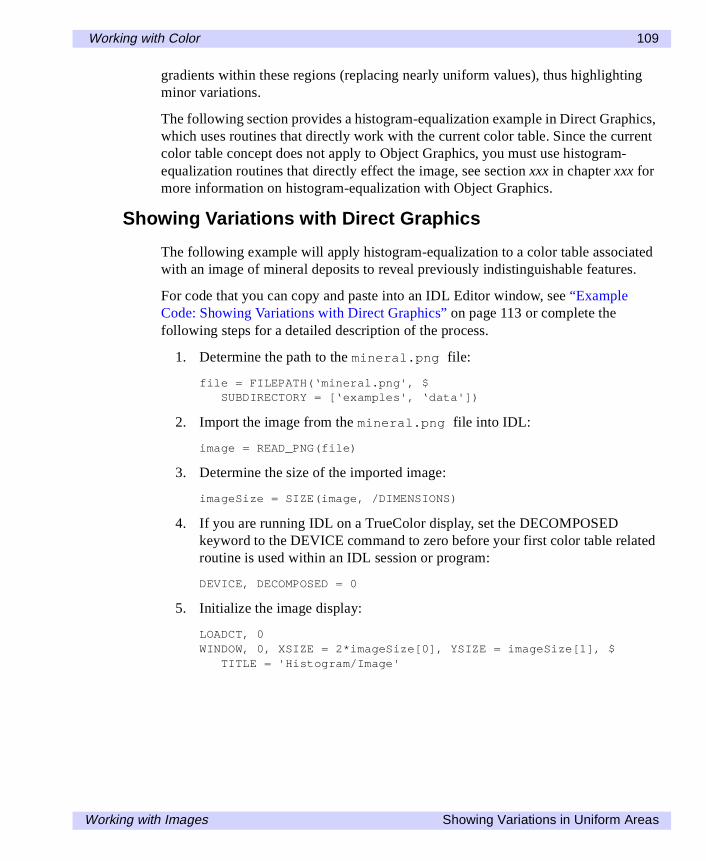
Working with Color 109
gradients within these regions (replacing nearly uniform values), thus highlightingminor variations.
The following section provides a histogram-equalization example in Direct Graphics,which uses routines that directly work with the current color table. Since the currentcolor table concept does not apply to Object Graphics, you must use histogram-equalization routines that directly effect the image, see section xxx in chapter xxx formore information on histogram-equalization with Object Graphics.
Showing Variations with Direct Graphics
The following example will apply histogram-equalization to a color table associatedwith an image of mineral deposits to reveal previously indistinguishable features.
For code that you can copy and paste into an IDL Editor window, see “ExampleCode: Showing Variations with Direct Graphics” on page 113 or complete thefollowing steps for a detailed description of the process.
1. Determine the path to the mineral.png file:
file = FILEPATH(‘mineral.png', $SUBDIRECTORY = [‘examples', ‘data'])
2. Import the image from the mineral.png file into IDL:
image = READ_PNG(file)
3. Determine the size of the imported image:
imageSize = SIZE(image, /DIMENSIONS)
4. If you are running IDL on a TrueColor display, set the DECOMPOSEDkeyword to the DEVICE command to zero before your first color table relatedroutine is used within an IDL session or program:
DEVICE, DECOMPOSED = 0
5. Initialize the image display:
LOADCT, 0WINDOW, 0, XSIZE = 2*imageSize[0], YSIZE = imageSize[1], $
TITLE = 'Histogram/Image'
Working with Images Showing Variations in Uniform Areas
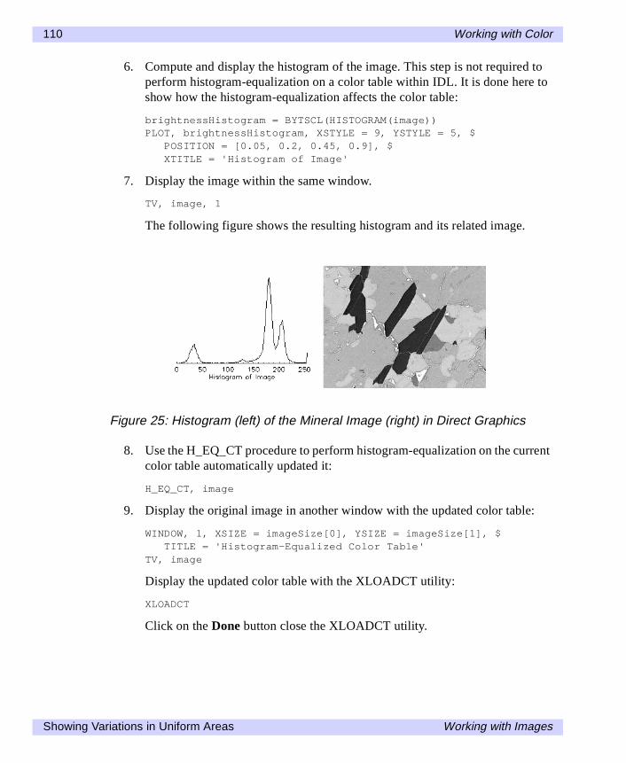
110 Working with Color
6. Compute and display the histogram of the image. This step is not required toperform histogram-equalization on a color table within IDL. It is done here toshow how the histogram-equalization affects the color table:
brightnessHistogram = BYTSCL(HISTOGRAM(image))PLOT, brightnessHistogram, XSTYLE = 9, YSTYLE = 5, $
POSITION = [0.05, 0.2, 0.45, 0.9], $XTITLE = 'Histogram of Image'
7. Display the image within the same window.
TV, image, 1
The following figure shows the resulting histogram and its related image.
8. Use the H_EQ_CT procedure to perform histogram-equalization on the currentcolor table automatically updated it:
H_EQ_CT, image
9. Display the original image in another window with the updated color table:
WINDOW, 1, XSIZE = imageSize[0], YSIZE = imageSize[1], $TITLE = 'Histogram-Equalized Color Table'
TV, image
Display the updated color table with the XLOADCT utility:
XLOADCT
Click on the Done button close the XLOADCT utility.
Figure 25: Histogram (left) of the Mineral Image (right) in Direct Graphics
Showing Variations in Uniform Areas Working with Images
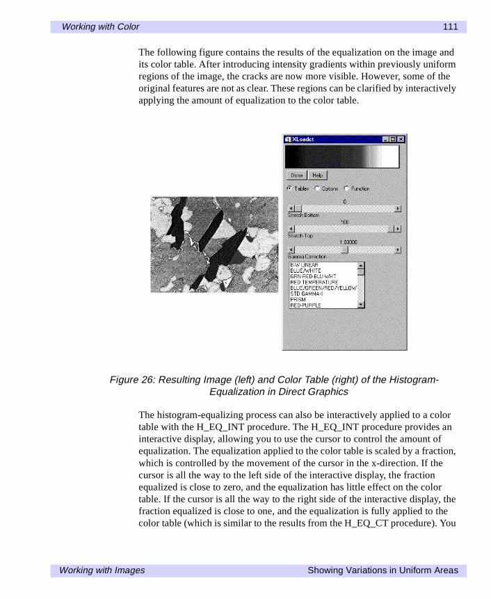
Working with Color 111
The following figure contains the results of the equalization on the image andits color table. After introducing intensity gradients within previously uniformregions of the image, the cracks are now more visible. However, some of theoriginal features are not as clear. These regions can be clarified by interactivelyapplying the amount of equalization to the color table.
The histogram-equalizing process can also be interactively applied to a colortable with the H_EQ_INT procedure. The H_EQ_INT procedure provides aninteractive display, allowing you to use the cursor to control the amount ofequalization. The equalization applied to the color table is scaled by a fraction,which is controlled by the movement of the cursor in the x-direction. If thecursor is all the way to the left side of the interactive display, the fractionequalized is close to zero, and the equalization has little effect on the colortable. If the cursor is all the way to the right side of the interactive display, thefraction equalized is close to one, and the equalization is fully applied to thecolor table (which is similar to the results from the H_EQ_CT procedure). You
Figure 26: Resulting Image (left) and Color Table (right) of the Histogram-Equalization in Direct Graphics
Working with Images Showing Variations in Uniform Areas
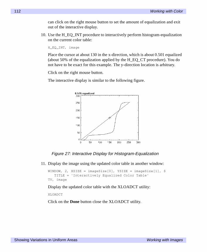
112 Working with Color
can click on the right mouse button to set the amount of equalization and exitout of the interactive display.
10. Use the H_EQ_INT procedure to interactively perform histogram-equalizationon the current color table:
H_EQ_INT, image
Place the cursor at about 130 in the x-direction, which is about 0.501 equalized(about 50% of the equalization applied by the H_EQ_CT procedure). You donot have to be exact for this example. The y-direction location is arbitrary.
Click on the right mouse button.
The interactive display is similar to the following figure.
11. Display the image using the updated color table in another window:
WINDOW, 2, XSIZE = imageSize[0], YSIZE = imageSize[1], $TITLE = 'Interactively Equalized Color Table'
TV, image
Display the updated color table with the XLOADCT utility:
XLOADCT
Click on the Done button close the XLOADCT utility.
Figure 27: Interactive Display for Histogram-Equalization
Showing Variations in Uniform Areas Working with Images
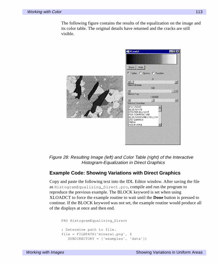
Working with Color 113
The following figure contains the results of the equalization on the image andits color table. The original details have returned and the cracks are stillvisible.
Example Code: Showing Variations with Direct Graphics
Copy and paste the following text into the IDL Editor window. After saving the fileas HistogramEqualizing_Direct.pro, compile and run the program toreproduce the previous example. The BLOCK keyword is set when usingXLOADCT to force the example routine to wait until the Done button is pressed tocontinue. If the BLOCK keyword was not set, the example routine would produce allof the displays at once and then end.
PRO HistogramEqualizing_Direct
; Determine path to file.file = FILEPATH('mineral.png', $
SUBDIRECTORY = ['examples', 'data'])
Figure 28: Resulting Image (left) and Color Table (right) of the InteractiveHistogram-Equalization in Direct Graphics
Working with Images Showing Variations in Uniform Areas
114 Working with Color
; Import image from file into IDL.image = READ_PNG(file)
; Determine size of imported image.imageSize = SIZE(image, /DIMENSIONS)
;Initialize IDL on a TrueColor display to use; color-related routines.DEVICE, DECOMPOSED = 0
; Initialize the image display.LOADCT, 0WINDOW, 0, XSIZE = 2*imageSize[0], YSIZE = imageSize[1], $
TITLE = 'Histogram/Image'
; Compute and scale histogram of image.brightnessHistogram = BYTSCL(HISTOGRAM(image))
; Display histogram plot.PLOT, brightnessHistogram, XSTYLE = 9, YSTYLE = 5, $
POSITION = [0.05, 0.2, 0.45, 0.9], $XTITLE = 'Histogram of Image'
; Display image.TV, image, 1
; Histogram-equalize the color table.H_EQ_CT, image
; Display image and updated color table in another; window.WINDOW, 1, XSIZE = imageSize[0], YSIZE = imageSize[1], $
TITLE = 'Histogram-Equalized Color Table'TV, image
; Display the updated color table with the XLOADCT; utility.XLOADCT, /BLOCK
; Interactively histogram-equalize the color table. The; H_EQ_INT routine provides an interactive display to; allow you to select the amount of equalization. Place; the cursor at about 130 in the x-direction, which is; about 0.501 equalized. The y-direction is arbitrary.; Click on the right mouse button.; NOTE: you do not have to be exact for this example.H_EQ_INT, image
Showing Variations in Uniform Areas Working with Images
Working with Color 115
; Display image and updated color table in another; window.WINDOW, 2, XSIZE = imageSize[0], YSIZE = imageSize[1], $
TITLE = 'Interactively Equalized Color Table'TV, image
; Display the updated color table with the XLOADCT; utility.XLOADCT, /BLOCK
END
Working with Images Showing Variations in Uniform Areas
116 Working with Color
Applying Color Annotations to Images
Many images are annotated to explain certain features or highlight specific details.Color annotations are more noticeable than plain black or white annotations. InDirect Graphics, how color annotations are applied depends on the type of image(indexed or RGB) displayed. With indexed images, annotation colors are derivedfrom the image’s associated color table. With RGB images, annotation colors areindependent of the RGB image in Direct Graphics. Annotation colors and images areseparated within Object Graphics regardless of the image type.
Applying Color Annotations to Indexed Images in DirectGraphics
Indexed images are usually associated with color tables. With Direct Graphics, theserelated color tables are used for all the colors shown within a display. Color tables aremade up of up to 256 color triples (red, green, and blue values of each color withinthe table). If you want to apply a specific color to data or to an annotation, you mustchange the red, green, and blue values at a specific index within the color table.
Color annotations are usually applied to label each color level within the image or toallow color comparisons. This section shows how to label each color level on anindexed image in Direct Graphics. As an example, an image of average worldtemperature is imported from the worldtmp.png file. This file does not contain acolor table associated with this image, so a pre-defined color table will be applied.This table provides the colors for the polygons and text used to make a colorbar forthis image. Each polygon uses the color of each level in the table. The text representsthe average temperature (in Celsius) of each level.
For code that you can copy and paste into an IDL Editor window, see “ExampleCode: Applying Color Annotations to Indexed Images in Direct Graphics” onpage 120 or complete the following steps for a detailed description of the process.
1. Determine the path to the worldtmp.png file:
worldtmpFile = FILEPATH('worldtmp.png', $SUBDIRECTORY = ['examples', 'demo', 'demodata'])
2. Import the image from the worldtmp.png file into IDL:
worldtmpImage = READ_PNG(worldtmpFile)
3. Determine the size of the imported image:
worldtmpSize = SIZE(worldtmpImage, /DIMENSIONS)
Applying Color Annotations to Images Working with Images
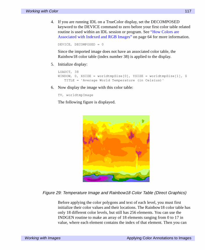
Working with Color 117
4. If you are running IDL on a TrueColor display, set the DECOMPOSEDkeyword to the DEVICE command to zero before your first color table relatedroutine is used within an IDL session or program. See “How Colors areAssociated with Indexed and RGB Images” on page 64 for more information.
DEVICE, DECOMPOSED = 0
Since the imported image does not have an associated color table, theRainbow18 color table (index number 38) is applied to the display.
5. Initialize display:
LOADCT, 38WINDOW, 0, XSIZE = worldtmpSize[0], YSIZE = worldtmpSize[1], $
TITLE = 'Average World Temperature (in Celsius)'
6. Now display the image with this color table:
TV, worldtmpImage
The following figure is displayed.
Before applying the color polygons and text of each level, you must firstinitialize their color values and their locations. The Rainbow18 color table hasonly 18 different color levels, but still has 256 elements. You can use theINDGEN routine to make an array of 18 elements ranging from 0 to 17 invalue, where each element contains the index of that element. Then you can
Figure 29: Temperature Image and Rainbow18 Color Table (Direct Graphics)
Working with Images Applying Color Annotations to Images
118 Working with Color
use the BYTSCL routine to scale these values to range from 0 to 255. Theresulting array contains the initial color value (from 0 to 255) of the associatedrange (from 0 to 17, equalling 18 elements).
7. Initialize the color level parameter:
fillColor = BYTSCL(INDGEN(18))
8. Initialize the average temperature of each level, which directly depends on theinitial color value of each range. Temperature is 0.20833 (5/24th) of the colorvalue. You can use this relationship to calculate the temperature and thenconvert it to a string variable to be used as text:
temperature = STRTRIM(FIX((5.*fillColor)/42.), 2)
NoteWhen the fillColor variable in the previous statement is multiplied by the floating-point value of 5 (denoted by the decimal after the number), the elements of the arrayare converted from byte values to floating-point values. These elements are thenconverted to integer values with the FIX routine so the decimal part will not bedisplayed. The STRTRIM routine converts the integer values to string values to bedisplayed as text. The second argument to STRTRIM is set to 2 to note the leadingand trailing blank characters should be trimmed away when the integer values areconverted to string values.
With the polygon color and text now defined, you can determine theirlocations. You can use the POLYFILL routine to draw each polygon and theXYOUTS routine to display each element of text. The process is repetitivefrom level to level, so a FOR/DO loop is used to display the entire colorbar.Since each polygon and text is drawn individually within the loop, you onlyneed to determine the location of a single polygon and an array of offsets foreach step in the loop. The following two steps describe this process.
9. Initialize the polygon and the text location parameters. Each polygon is 25pixels in width and 18 pixels in height. The offset will move the y-location 18pixels every time a new polygon is displayed:
x = [5., 30., 30., 5., 5.]y = [5., 5., 23., 23., 5.] + 5.offset = 18.*FINDGEN(19) + 5.
Applying Color Annotations to Images Working with Images
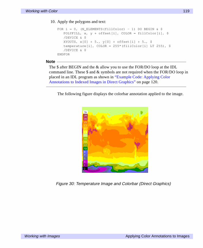
Working with Color 119
10. Apply the polygons and text:
FOR i = 0, (N_ELEMENTS(fillColor) - 1) DO BEGIN & $POLYFILL, x, y + offset[i], COLOR = fillColor[i], $/DEVICE & $XYOUTS, x[0] + 5., y[0] + offset[i] + 5., $temperature[i], COLOR = 255*(fillColor[i] LT 255), $/DEVICE & $
ENDFOR
NoteThe $ after BEGIN and the & allow you to use the FOR/DO loop at the IDLcommand line. These $ and & symbols are not required when the FOR/DO loop inplaced in an IDL program as shown in “Example Code: Applying ColorAnnotations to Indexed Images in Direct Graphics” on page 120.
The following figure displays the colorbar annotation applied to the image.
Figure 30: Temperature Image and Colorbar (Direct Graphics)
Working with Images Applying Color Annotations to Images
120 Working with Color
Example Code: Applying Color Annotations to Indexed Images inDirect Graphics
Copy and paste the following text into the IDL Editor window. After saving the fileas ApplyColorbar_Indexed_Direct.pro, compile and run the program toreproduce the previous example.
PRO ApplyColorbar_Indexed_Direct
; Determine path to "worldtmp.png" file.worldtmpFile = FILEPATH('worldtmp.png', $
SUBDIRECTORY = ['examples', 'demo', 'demodata'])
; Import image from file into IDL.worldtmpImage = READ_PNG(worldtmpFile)
; Determine size of imported image.worldtmpSize = SIZE(worldtmpImage, /DIMENSIONS)
; Initialize display.DEVICE, DECOMPOSED = 0LOADCT, 38WINDOW, 0, XSIZE = worldtmpSize[0], $
YSIZE = worldtmpSize[1], $TITLE = 'Average World Temperature (in Celsius)'
; Display image.TV, worldtmpImage
; Initialize color level parameter.fillColor = BYTSCL(INDGEN(18))
; Initialize text variable.temperature = STRTRIM(FIX((5.*fillColor)/42.), 2)
; Initialize polygon and text location parameters.x = [5., 30., 30., 5., 5.]y = [5., 5., 23., 23., 5.] + 5.offset = 18.*FINDGEN(19) + 5.
; Apply polygons and text.FOR i = 0, (N_ELEMENTS(fillColor) - 1) DO BEGIN
POLYFILL, x, y + offset[i], COLOR = fillColor[i], $/DEVICEXYOUTS, x[0] + 5., y[0] + offset[i] + 5., $temperature[i], COLOR = 255*(fillColor[i] LT 255), $/DEVICE
Applying Color Annotations to Images Working with Images
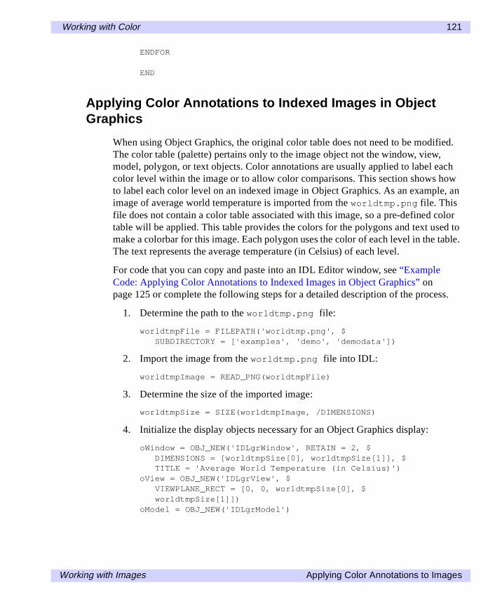
Working with Color 121
ENDFOR
END
Applying Color Annotations to Indexed Images in ObjectGraphics
When using Object Graphics, the original color table does not need to be modified.The color table (palette) pertains only to the image object not the window, view,model, polygon, or text objects. Color annotations are usually applied to label eachcolor level within the image or to allow color comparisons. This section shows howto label each color level on an indexed image in Object Graphics. As an example, animage of average world temperature is imported from the worldtmp.png file. Thisfile does not contain a color table associated with this image, so a pre-defined colortable will be applied. This table provides the colors for the polygons and text used tomake a colorbar for this image. Each polygon uses the color of each level in the table.The text represents the average temperature (in Celsius) of each level.
For code that you can copy and paste into an IDL Editor window, see “ExampleCode: Applying Color Annotations to Indexed Images in Object Graphics” onpage 125 or complete the following steps for a detailed description of the process.
1. Determine the path to the worldtmp.png file:
worldtmpFile = FILEPATH('worldtmp.png', $SUBDIRECTORY = ['examples', 'demo', 'demodata'])
2. Import the image from the worldtmp.png file into IDL:
worldtmpImage = READ_PNG(worldtmpFile)
3. Determine the size of the imported image:
worldtmpSize = SIZE(worldtmpImage, /DIMENSIONS)
4. Initialize the display objects necessary for an Object Graphics display:
oWindow = OBJ_NEW('IDLgrWindow', RETAIN = 2, $DIMENSIONS = [worldtmpSize[0], worldtmpSize[1]], $TITLE = 'Average World Temperature (in Celsius)')
oView = OBJ_NEW('IDLgrView', $VIEWPLANE_RECT = [0, 0, worldtmpSize[0], $worldtmpSize[1]])
oModel = OBJ_NEW('IDLgrModel')
Working with Images Applying Color Annotations to Images
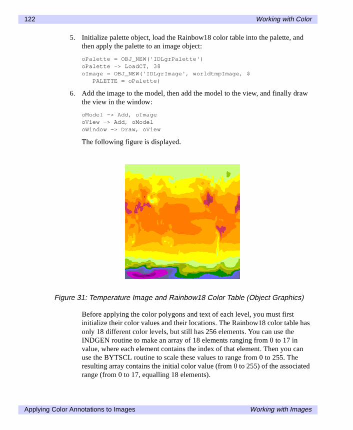
122 Working with Color
5. Initialize palette object, load the Rainbow18 color table into the palette, andthen apply the palette to an image object:
oPalette = OBJ_NEW('IDLgrPalette')oPalette -> LoadCT, 38oImage = OBJ_NEW('IDLgrImage', worldtmpImage, $
PALETTE = oPalette)
6. Add the image to the model, then add the model to the view, and finally drawthe view in the window:
oModel -> Add, oImageoView -> Add, oModeloWindow -> Draw, oView
The following figure is displayed.
Before applying the color polygons and text of each level, you must firstinitialize their color values and their locations. The Rainbow18 color table hasonly 18 different color levels, but still has 256 elements. You can use theINDGEN routine to make an array of 18 elements ranging from 0 to 17 invalue, where each element contains the index of that element. Then you canuse the BYTSCL routine to scale these values to range from 0 to 255. Theresulting array contains the initial color value (from 0 to 255) of the associatedrange (from 0 to 17, equalling 18 elements).
Figure 31: Temperature Image and Rainbow18 Color Table (Object Graphics)
Applying Color Annotations to Images Working with Images
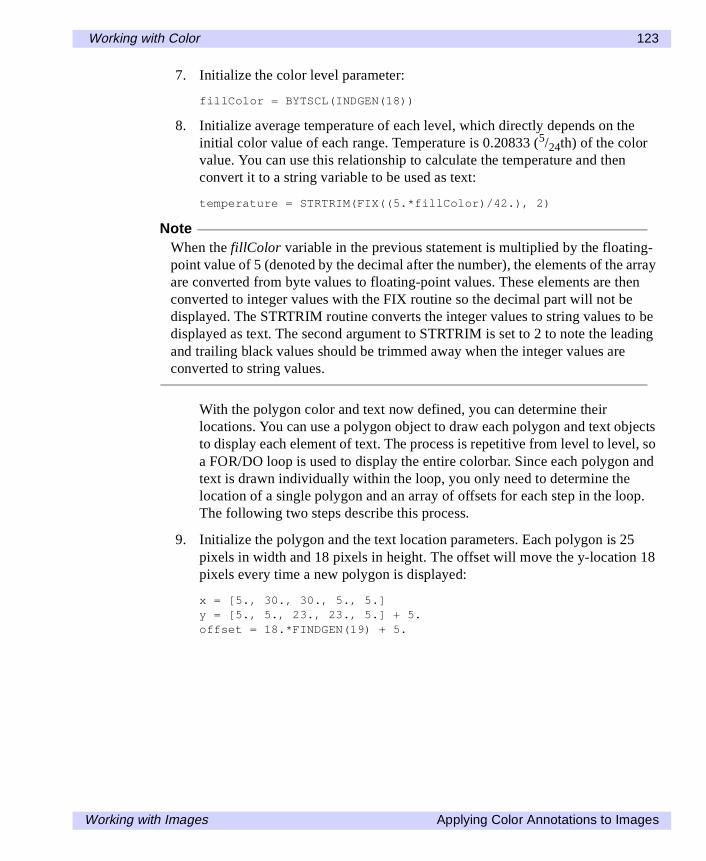
Working with Color 123
7. Initialize the color level parameter:
fillColor = BYTSCL(INDGEN(18))
8. Initialize average temperature of each level, which directly depends on theinitial color value of each range. Temperature is 0.20833 (5/24th) of the colorvalue. You can use this relationship to calculate the temperature and thenconvert it to a string variable to be used as text:
temperature = STRTRIM(FIX((5.*fillColor)/42.), 2)
NoteWhen the fillColor variable in the previous statement is multiplied by the floating-point value of 5 (denoted by the decimal after the number), the elements of the arrayare converted from byte values to floating-point values. These elements are thenconverted to integer values with the FIX routine so the decimal part will not bedisplayed. The STRTRIM routine converts the integer values to string values to bedisplayed as text. The second argument to STRTRIM is set to 2 to note the leadingand trailing black values should be trimmed away when the integer values areconverted to string values.
With the polygon color and text now defined, you can determine theirlocations. You can use a polygon object to draw each polygon and text objectsto display each element of text. The process is repetitive from level to level, soa FOR/DO loop is used to display the entire colorbar. Since each polygon andtext is drawn individually within the loop, you only need to determine thelocation of a single polygon and an array of offsets for each step in the loop.The following two steps describe this process.
9. Initialize the polygon and the text location parameters. Each polygon is 25pixels in width and 18 pixels in height. The offset will move the y-location 18pixels every time a new polygon is displayed:
x = [5., 30., 30., 5., 5.]y = [5., 5., 23., 23., 5.] + 5.offset = 18.*FINDGEN(19) + 5.
Working with Images Applying Color Annotations to Images
124 Working with Color
10. Initialize the polygon and text objects:
oPolygon = OBJARR(18)oText = OBJARR(18)FOR i = 0, (N_ELEMENTS(oPolygon) - 1) DO BEGIN & $
oPolygon[i] = OBJ_NEW('IDLgrPolygon', x, $y + offset[i], COLOR = fillColor[i], $PALETTE = oPalette) & $oText[i] = OBJ_NEW('IDLgrText', temperature[i], $LOCATIONS = [x[0] + 3., y[0] + offset[i] + 3.], $COLOR = 255*(fillColor[i] LT 255), $PALETTE = oPalette) & $
ENDFOR
NoteThe $ after BEGIN and the & allow you to use the FOR/DO loop at the IDLcommand line. These $ and & symbols are not required when the FOR/DO loop inplaced in an IDL program as shown in “Example Code: Applying ColorAnnotations to Indexed Images in Object Graphics” on page 125.
11. Add the polygons and text to the model, then add the model to the view, andfinally redraw the view in the window:
oModel -> Add, oPolygonoModel -> Add, oTextoWindow -> Draw, oView
Applying Color Annotations to Images Working with Images
Working with Color 125
The following figure displays the colorbar annotation applied to the image.
12. Clean-up object references. When working with objects always remember toclean-up any object references with the OBJ_DESTROY routine. Since theview contains all the other objects, except for the window (which is destroyedby the user), you only need to use OBJ_DESTROY on the view and the paletteobjects:
OBJ_DESTROY, [oView, oPalette]
Example Code: Applying Color Annotations to Indexed Images inObject Graphics
Copy and paste the following text into the IDL Editor window. After saving the fileas ApplyColorbar_Indexed_Object.pro, compile and run the program toreproduce the previous example.
PRO ApplyColorbar_Indexed_Object
; Determine path to "worldtmp.png" file.worldtmpFile = FILEPATH('worldtmp.png', $
SUBDIRECTORY = ['examples', 'demo', 'demodata'])
; Import image from file into IDL.worldtmpImage = READ_PNG(worldtmpFile)
Figure 32: Temperature Image and Colorbar (Object Graphics
Working with Images Applying Color Annotations to Images
126 Working with Color
; Determine size of imported image.worldtmpSize = SIZE(worldtmpImage, /DIMENSIONS)
; Initialize objects.; Initialize display.oWindow = OBJ_NEW('IDLgrWindow', RETAIN = 2, $
DIMENSIONS = [worldtmpSize[0], worldtmpSize[1]], $TITLE = 'Average World Temperature (in Celsius)')
oView = OBJ_NEW('IDLgrView', $VIEWPLANE_RECT = [0, 0, worldtmpSize[0], $worldtmpSize[1]])
oModel = OBJ_NEW('IDLgrModel'); Initialize palette and image.oPalette = OBJ_NEW('IDLgrPalette')oPalette -> LoadCT, 38oImage = OBJ_NEW('IDLgrImage', worldtmpImage, $
PALETTE = oPalette)
; Add image to model, which is added to view, and then; display view in window.oModel -> Add, oImageoView -> Add, oModeloWindow -> Draw, oView
; Initialize color level parameter.fillColor = BYTSCL(INDGEN(18))
; Initialize text variable.temperature = STRTRIM(FIX((5*fillColor)/42), 2)
; Initialize polygon and text location parameters.x = [5., 30., 30., 5., 5.]y = [5., 5., 23., 23., 5.] + 5.offset = 18.*FINDGEN(19) + 5.
; Initialize polygon and text objects.oPolygon = OBJARR(18)oText = OBJARR(18)FOR i = 0, (N_ELEMENTS(oPolygon) - 1) DO BEGIN
oPolygon[i] = OBJ_NEW('IDLgrPolygon', x, $y + offset[i], COLOR = fillColor[i], $PALETTE = oPalette)oText[i] = OBJ_NEW('IDLgrText', temperature[i], $LOCATIONS = [x[0] + 3., y[0] + offset[i] + 3.], $COLOR = 255*(fillColor[i] LT 255), $PALETTE = oPalette)
ENDFOR
; Add polygons and text to model and then re-display
Applying Color Annotations to Images Working with Images
Working with Color 127
; view in window.oModel -> Add, oPolygonoModel -> Add, oTextoWindow -> Draw, oView
; Clean-up object references.OBJ_DESTROY, [oView, oPalette]
END
Applying Color Annotations to RGB Images in DirectGraphics
RGB images contain their own color information. Color tables do not apply to RGBimages. With Direct Graphics the color of the annotations on an RGB image do notdepend on a color table.
TipIf you are running IDL on a PseudoColor display, use the COLOR_QUAN routineto convert the RGB image to an indexed image with an associated color table todisplay the image and see the previous section, “Applying Color Annotations toIndexed Images in Direct Graphics” on page 116.
If you want to apply a specific color to data or an annotation, you must provide theTrueColor index for that color. The TrueColor index ranges from 0 to 16,777,216.You can derive a TrueColor index from its red, green, and blue values:
red = 255green = 128blue = 0trueColorIndex = red + (256L*green) + ((256L^2)*blue)PRINT, trueColorIndex
33023
where red, green, and blue are either scalars or vectors of values ranging from 0 to255 and representing the amount of red, green, and blue in the resulting color. The Lafter the numbers defines that number as a longword integer data type. The abovered, green, and blue combination creates the color of orange, which has a TrueColorindex of 33,023.
In this example, a color spectrum of additive and subtractive primary colors will bedrawn on an RGB image for comparison with the colors in an image. Theglowing_gas.jpg file contains an RGB image of an expanding shell of glowing
Working with Images Applying Color Annotations to Images
128 Working with Color
gas surrounding a hot, massive star in our Milky Way Galaxy. This image contains allthe colors of this spectrum.
For code that you can copy and paste into an IDL Editor window, see “ExampleCode: Applying Color Annotations to Indexed Images in Direct Graphics” onpage 120 or complete the following steps for a detailed description of the process.
1. Determine the path to the glowing_gas.jpg file:
cosmicFile = FILEPATH('glowing_gas.jpg', $SUBDIRECTORY = ['examples', 'data'])
2. Import the image from the glowing_gas.jpg file into IDL:
READ_JPEG, cosmicFile, cosmicImage
3. Determine the size of the imported image. The image contained within this fileis pixel-interleaved (the color information is contained within the firstdimension). You can use the SIZE routine to determine the other dimensions ofthis image:
cosmicSize = SIZE(cosmicImage, /DIMENSIONS)
4. If you are running IDL on a TrueColor display, set the DECOMPOSEDkeyword to the DEVICE command to one before your first RGB image isdisplayed within an IDL session or program. See “How Colors are Associatedwith Indexed and RGB Images” on page 64 for more information:
DEVICE, DECOMPOSED = 1
5. Use the dimensions determined in the previous step to initialize the display:
WINDOW, 0, XSIZE = cosmicSize[1], YSIZE = cosmicSize[2], $TITLE = ‘glowing_gas.jpg'
6. Now display the image with the TRUE keyword set to 1 since the image ispixel interleaved:
TV, cosmicImage, TRUE = 1
The following figure shows that the image contains all of the colors of theadditive and subtractive primary spectrum. In the following steps, a colorbar
Applying Color Annotations to Images Working with Images
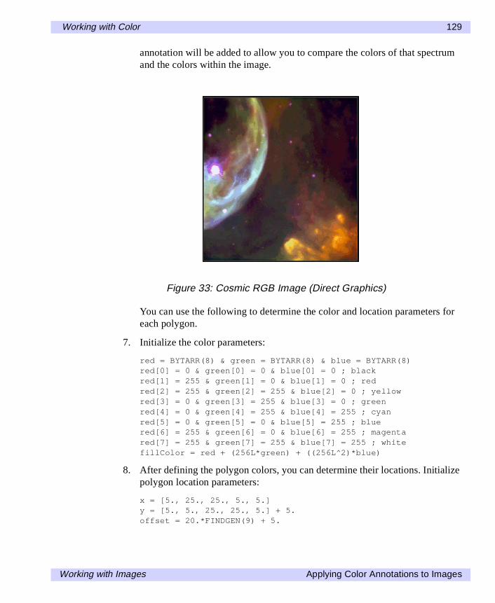
Working with Color 129
annotation will be added to allow you to compare the colors of that spectrumand the colors within the image.
You can use the following to determine the color and location parameters foreach polygon.
7. Initialize the color parameters:
red = BYTARR(8) & green = BYTARR(8) & blue = BYTARR(8)red[0] = 0 & green[0] = 0 & blue[0] = 0 ; blackred[1] = 255 & green[1] = 0 & blue[1] = 0 ; redred[2] = 255 & green[2] = 255 & blue[2] = 0 ; yellowred[3] = 0 & green[3] = 255 & blue[3] = 0 ; greenred[4] = 0 & green[4] = 255 & blue[4] = 255 ; cyanred[5] = 0 & green[5] = 0 & blue[5] = 255 ; bluered[6] = 255 & green[6] = 0 & blue[6] = 255 ; magentared[7] = 255 & green[7] = 255 & blue[7] = 255 ; whitefillColor = red + (256L*green) + ((256L^2)*blue)
8. After defining the polygon colors, you can determine their locations. Initializepolygon location parameters:
x = [5., 25., 25., 5., 5.]y = [5., 5., 25., 25., 5.] + 5.offset = 20.*FINDGEN(9) + 5.
Figure 33: Cosmic RGB Image (Direct Graphics)
Working with Images Applying Color Annotations to Images
130 Working with Color
The x and y variables pertain to the x and y locations (in pixel units) of eachbox of color. The offset maintains the spacing (in pixel units) of each box.Since the image is made up of mostly a black background, the x border of thecolorbar is also determined to draw a white border around the polygons.
9. Initialize location of colorbar border:
x_border = [x[0] + offset[0], x[1] + offset[7], $x[2] + offset[7], x[3] + offset[0], x[4] + offset[0]]
The y border is already defined by the y variable.
These parameters are used with POLYFILL and PLOTS to draw the boxes ofthe color spectrum and the colorbar border. Each polygon is 20 pixels wide and20 pixels high. The offset will move the y-location 20 pixels every time a newpolygon is displayed.
10. Apply the polygons and border. You can use the POLYFILL routine to draweach polygon. The process is repetitive from level to level, so a FOR/DO loopis used to display the entire colorbar. Since each polygon is drawn individuallywithin the loop, you only need to determine the location of a single polygonand an array of offsets for each step in the loop:
FOR i = 0, (N_ELEMENTS(fillColor) - 1) DO POLYFILL, $x + offset[i], y, COLOR = fillColor[i], /DEVICE
PLOTS, x_border, y, COLOR = fillColor[7], /DEVICE
Applying Color Annotations to Images Working with Images
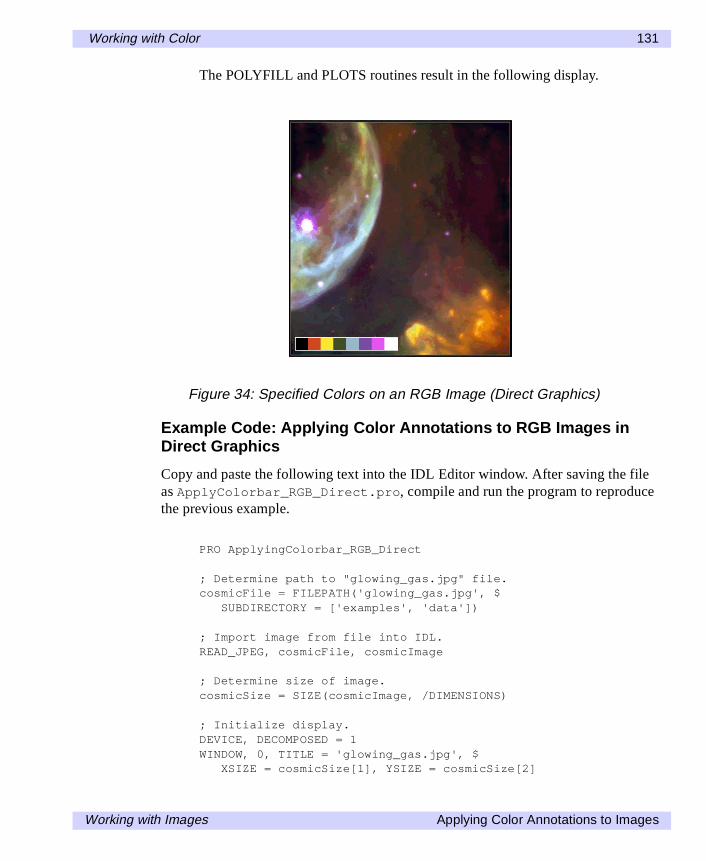
Working with Color 131
The POLYFILL and PLOTS routines result in the following display.
Example Code: Applying Color Annotations to RGB Images inDirect Graphics
Copy and paste the following text into the IDL Editor window. After saving the fileas ApplyColorbar_RGB_Direct.pro, compile and run the program to reproducethe previous example.
PRO ApplyingColorbar_RGB_Direct
; Determine path to "glowing_gas.jpg" file.cosmicFile = FILEPATH('glowing_gas.jpg', $
SUBDIRECTORY = ['examples', 'data'])
; Import image from file into IDL.READ_JPEG, cosmicFile, cosmicImage
; Determine size of image.cosmicSize = SIZE(cosmicImage, /DIMENSIONS)
; Initialize display.DEVICE, DECOMPOSED = 1WINDOW, 0, TITLE = 'glowing_gas.jpg', $
XSIZE = cosmicSize[1], YSIZE = cosmicSize[2]
Figure 34: Specified Colors on an RGB Image (Direct Graphics)
Working with Images Applying Color Annotations to Images
132 Working with Color
; Diplay image.TV, cosmicImage, TRUE = 1
; Initialize color parameters.red = BYTARR(8) & green = BYTARR(8) & blue = BYTARR(8)red[0] = 0 & green[0] = 0 & blue[0] = 0 ; blackred[1] = 255 & green[1] = 0 & blue[1] = 0 ; redred[2] = 255 & green[2] = 255 & blue[2] = 0 ; yellowred[3] = 0 & green[3] = 255 & blue[3] = 0 ; greenred[4] = 0 & green[4] = 255 & blue[4] = 255 ; cyanred[5] = 0 & green[5] = 0 & blue[5] = 255 ; bluered[6] = 255 & green[6] = 0 & blue[6] = 255 ; magentared[7] = 255 & green[7] = 255 & blue[7] = 255 ; whitefillColor = red + (256L*green) + ((256L^2)*blue)
; Initialize polygon location parameters.x = [5., 25., 25., 5., 5.]y = [5., 5., 25., 25., 5.] + 5.offset = 20.*FINDGEN(9) + 5.
; Initialize location of colorbar border.x_border = [x[0] + offset[0], x[1] + offset[7], $
x[2] + offset[7], x[3] + offset[0], x[4] + offset[0]]
; Apply polygons and border.FOR i = 0, (N_ELEMENTS(fillColor) - 1) DO POLYFILL, $
x + offset[i], y, COLOR = fillColor[i], /DEVICEPLOTS, x_border, y, /DEVICE, COLOR = fillColor[7]
END
Applying Color Annotations to RGB Images in ObjectGraphics
When using Object Graphics, colors can be defined just by their red, green, and bluevalues. The TrueColor index conversion equation is not required for Object Graphics.In this example, a color spectrum of additive and subtractive primary colors will bedrawn on an RGB image for comparison with the colors in that image. Theglowing_gas.jpg file contains an RGB image of an expanding shell of glowinggas surrounding a hot, massive star in our Milky Way Galaxy. This image contains allthe colors of this spectrum.
For code that you can copy and paste into an IDL Editor window, see “ExampleCode: Applying Color Annotations to RGB Images in Object Graphics” on page 136or complete the following steps for a detailed description of the process.
Applying Color Annotations to Images Working with Images
Working with Color 133
1. Determine the path to the glowing_gas.jpg file:
cosmicFile = FILEPATH('glowing_gas.jpg', $SUBDIRECTORY = ['examples', 'data'])
2. Import the image from the glowing_gas.jpg file into IDL:
READ_JPEG, cosmicFile, cosmicImage
3. Determine the size of the imported image. The image contained within this fileis pixel-interleaved (the color information is contained within the firstdimension). You can use the SIZE routine to determine the other dimensions ofthis image:
cosmicSize = SIZE(cosmicImage, /DIMENSIONS)
4. Initialize the display objects required for an Object Graphics display:
oWindow = OBJ_NEW('IDLgrWindow', RETAIN = 2, $DIMENSIONS = [cosmicSize[1], cosmicSize[2]], $TITLE = 'glowing_gas.jpeg')
oView = OBJ_NEW('IDLgrView', $VIEWPLANE_RECT = [0., 0., cosmicSize[1], $cosmicSize[2]])
oModel = OBJ_NEW('IDLgrModel')
5. Initialize the image object. The INTERLEAVE keyword is set to 0 because theRGB image is pixel-interleaved:
oImage = OBJ_NEW('IDLgrImage', cosmicImage, $INTERLEAVE = 0, DIMENSIONS = [cosmicSize[1], $cosmicSize[2]])
6. Add the image to the model, then add the model to the view, and finally drawthe view in the window:
oModel -> Add, oImageoView -> Add, oModeloWindow -> Draw, oView
The following image contains all of the colors of the additive and subtractiveprimary spectrum. A colorbar annotation can be added to compare the colors
Working with Images Applying Color Annotations to Images
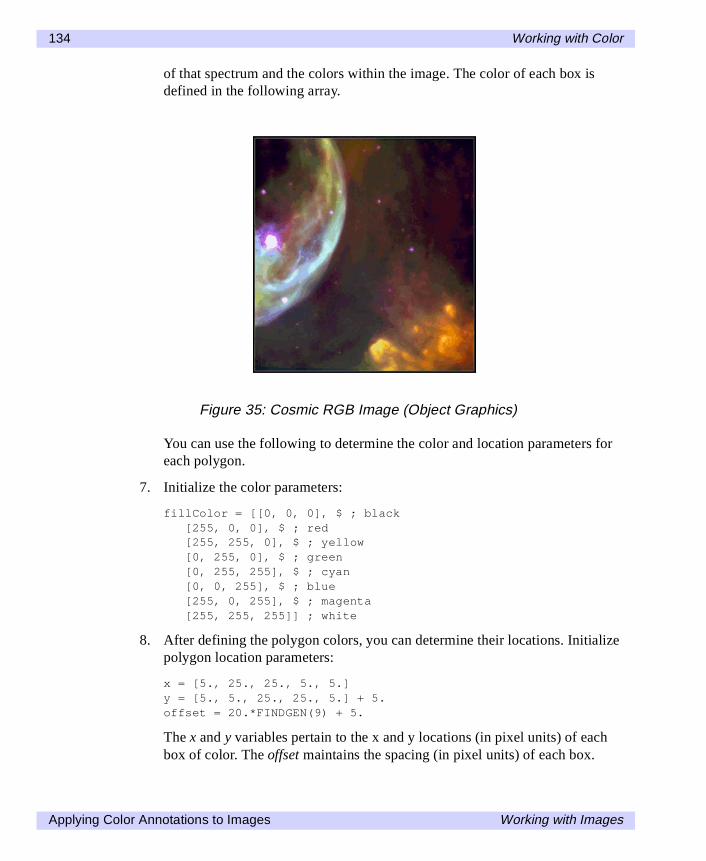
134 Working with Color
of that spectrum and the colors within the image. The color of each box isdefined in the following array.
You can use the following to determine the color and location parameters foreach polygon.
7. Initialize the color parameters:
fillColor = [[0, 0, 0], $ ; black[255, 0, 0], $ ; red[255, 255, 0], $ ; yellow[0, 255, 0], $ ; green[0, 255, 255], $ ; cyan[0, 0, 255], $ ; blue[255, 0, 255], $ ; magenta[255, 255, 255]] ; white
8. After defining the polygon colors, you can determine their locations. Initializepolygon location parameters:
x = [5., 25., 25., 5., 5.]y = [5., 5., 25., 25., 5.] + 5.offset = 20.*FINDGEN(9) + 5.
The x and y variables pertain to the x and y locations (in pixel units) of eachbox of color. The offset maintains the spacing (in pixel units) of each box.
Figure 35: Cosmic RGB Image (Object Graphics)
Applying Color Annotations to Images Working with Images
Working with Color 135
Since the image is made up of mostly a black background, the x border of thecolorbar is also determined to draw a white border around the polygons.
9. Initialize location of colorbar border:
x_border = [x[0] + offset[0], x[1] + offset[7], $x[2] + offset[7], x[3] + offset[0], x[4] + offset[0]]
The y border is already defined by the y variable.
These parameters are used when initializing the polygon and polyline objectsThese objects will be used draw the boxes of the color spectrum and thecolorbar border. Each polygon is 20 pixels wide and 20 pixels high. The offsetwill move the y-location 20 pixels every time a new polygon is displayed.
10. Initialize the polygon objects. The process is repetitive from level to level, so aFOR/DO loop will be used to display the entire colorbar. Since each polygon isdrawn individually within the loop, you only need to determine the location ofa single polygon and an array of offsets for each step in the loop:
oPolygon = OBJARR(8)FOR i = 0, (N_ELEMENTS(oPolygon) - 1) DO oPolygon[i] = $
OBJ_NEW('IDLgrPolygon', x + offset[i], y, $COLOR = fillColor[*, i])
11. The colorbar border is produced with a polyline object. This polyline objectrequires a z variable to define it slightly above the polygons and image. The zvariable is required to place the polyline in front of the polygons. Initializepolyline (border) object:
z = [0.001, 0.001, 0.001, 0.001, 0.001]oPolyline = OBJ_NEW('IDLgrPolyline', x_border, y, z, $
COLOR = [255, 255, 255])
12. The polygon and polyline objects can now be added to the model and thendisplayed (re-drawn) in the window. Add the polygons and polyline to themodel, then add the model to the view, and finally redraw the view in thewindow:
oModel -> Add, oPolygonoModel -> Add, oPolylineoWindow -> Draw, oView
Working with Images Applying Color Annotations to Images
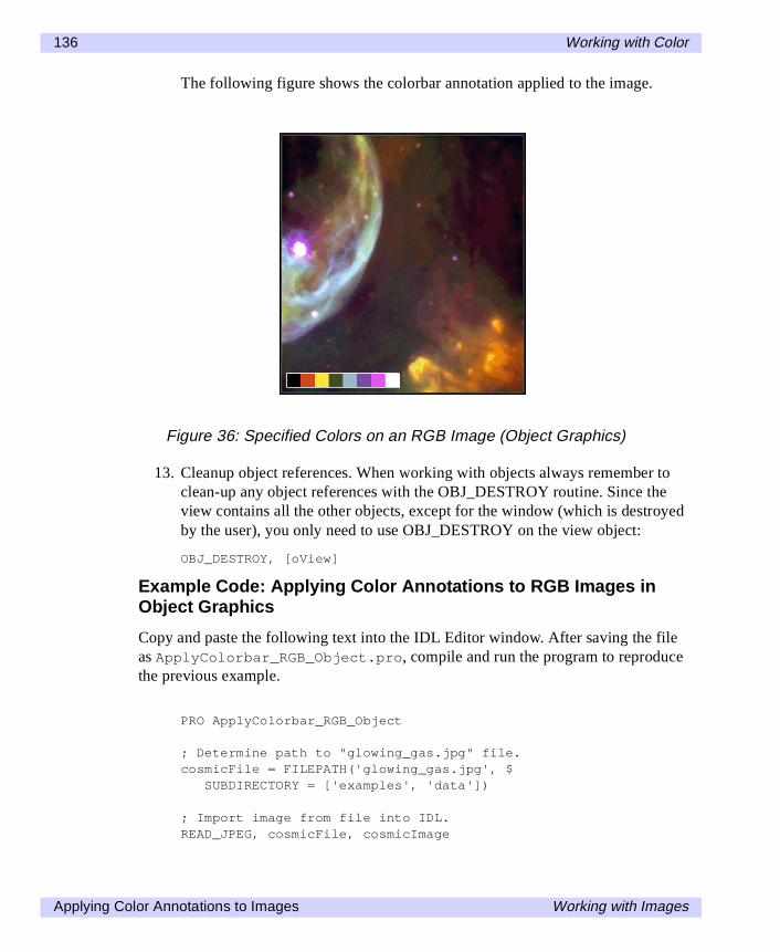
136 Working with Color
The following figure shows the colorbar annotation applied to the image.
13. Cleanup object references. When working with objects always remember toclean-up any object references with the OBJ_DESTROY routine. Since theview contains all the other objects, except for the window (which is destroyedby the user), you only need to use OBJ_DESTROY on the view object:
OBJ_DESTROY, [oView]
Example Code: Applying Color Annotations to RGB Images inObject Graphics
Copy and paste the following text into the IDL Editor window. After saving the fileas ApplyColorbar_RGB_Object.pro, compile and run the program to reproducethe previous example.
PRO ApplyColorbar_RGB_Object
; Determine path to "glowing_gas.jpg" file.cosmicFile = FILEPATH('glowing_gas.jpg', $
SUBDIRECTORY = ['examples', 'data'])
; Import image from file into IDL.READ_JPEG, cosmicFile, cosmicImage
Figure 36: Specified Colors on an RGB Image (Object Graphics)
Applying Color Annotations to Images Working with Images
Working with Color 137
; Determine size of image.cosmicSize = SIZE(cosmicImage, /DIMENSIONS)
; Initialize objects.; Initialize display.oWindow = OBJ_NEW('IDLgrWindow', RETAIN = 2, $
DIMENSIONS = [cosmicSize[1], cosmicSize[2]], $TITLE = 'glowing_gas.jpg')
oView = OBJ_NEW('IDLgrView', $VIEWPLANE_RECT = [0., 0., cosmicSize[1], $cosmicSize[2]])
oModel = OBJ_NEW('IDLgrModel'); Initialize image.oImage = OBJ_NEW('IDLgrImage', cosmicImage, $
INTERLEAVE = 0, DIMENSIONS = [cosmicSize[1], $cosmicSize[2]])
; Add image to model, which is added to view, and then; display view in window.oModel -> Add, oImageoView -> Add, oModeloWindow -> Draw, oView
; Initialize color parameter.fillColor = [[0, 0, 0], $ ; black
[255, 0, 0], $ ; red[255, 255, 0], $ ; yellow[0, 255, 0], $ ; green[0, 255, 255], $ ; cyan[0, 0, 255], $ ; blue[255, 0, 255], $ ; magenta[255, 255, 255]] ; white
; Initialize polygon location parameters.x = [5., 25., 25., 5., 5.]y = [5., 5., 25., 25., 5.] + 5.offset = 20.*FINDGEN(9) + 5.
; Initialize location of colorbar border.x_border = [x[0] + offset[0], x[1] + offset[7], $
x[2] + offset[7], x[3] + offset[0], x[4] + offset[0]]
; Initialize polygon objects.oPolygon = OBJARR(8)FOR i = 0, (N_ELEMENTS(oPolygon) - 1) DO oPolygon[i] = $
OBJ_NEW('IDLgrPolygon', x + offset[i], y, $COLOR = fillColor[*, i])
; Initialize polyline (border) object.
Working with Images Applying Color Annotations to Images
138 Working with Color
z = [0.001, 0.001, 0.001, 0.001, 0.001]oPolyline = OBJ_NEW('IDLgrPolyline', x_border, y, z, $
COLOR = [255, 255, 255])
; Add polgons and polyline to model and then re-display; view in window.oModel -> Add, oPolygonoModel -> Add, oPolylineoWindow -> Draw, oView
; Clean-up object references.OBJ_DESTROY, [oView]
END
Applying Color Annotations to Images Working with Images