Excel on Steroids Tips Booklet - Ningapi.ning.com/files/bKgApL8YprvhAANHDOVBfRiariL0M0... · Excel on Steroids Tips Booklet | 1 ... Navigating pg 2 PivotTable pg 3 Functions pg 4

Excel on Steroids Tips Booklet

EXCLUSIVE TO PASTEL BUSINESS INTELLEGENCE CUSTOMERS

Excel on Steroids Tips Booklet | 1

CONTENTS

Toolbars pg 2

Navigating pg 2

PivotTable pg 3

Functions pg 4

Charts pg 8

Filtering pg 8

Formatting pg 9

Conditional Formatting pg 11

Shortcuts pg 13

Page Setup pg 13

Hyperlinks pg 15

Excel Options pg 15

Sorting pg 15

Subtotals pg 16

The power of Excel with its immense functionality can be quite daunting to many business users. The Excel onSteroids tips booklet has 50 carefully selected gems to help you perform those “everyday Excel” tasks moreefficiently. Over 7000 companies currently using the Pastel Business Intelligence Centre Module have contributedover the years to ensure we accumulate tips and tricks appropriate to using Excel as a powerful business reportingtool. We hope you enjoy it.

To take your Excel skills to the next level, go http://www.pastel.co.za/auditor/academy.asp to find out about theExcel on Steroids workshops.

TOOLBARS

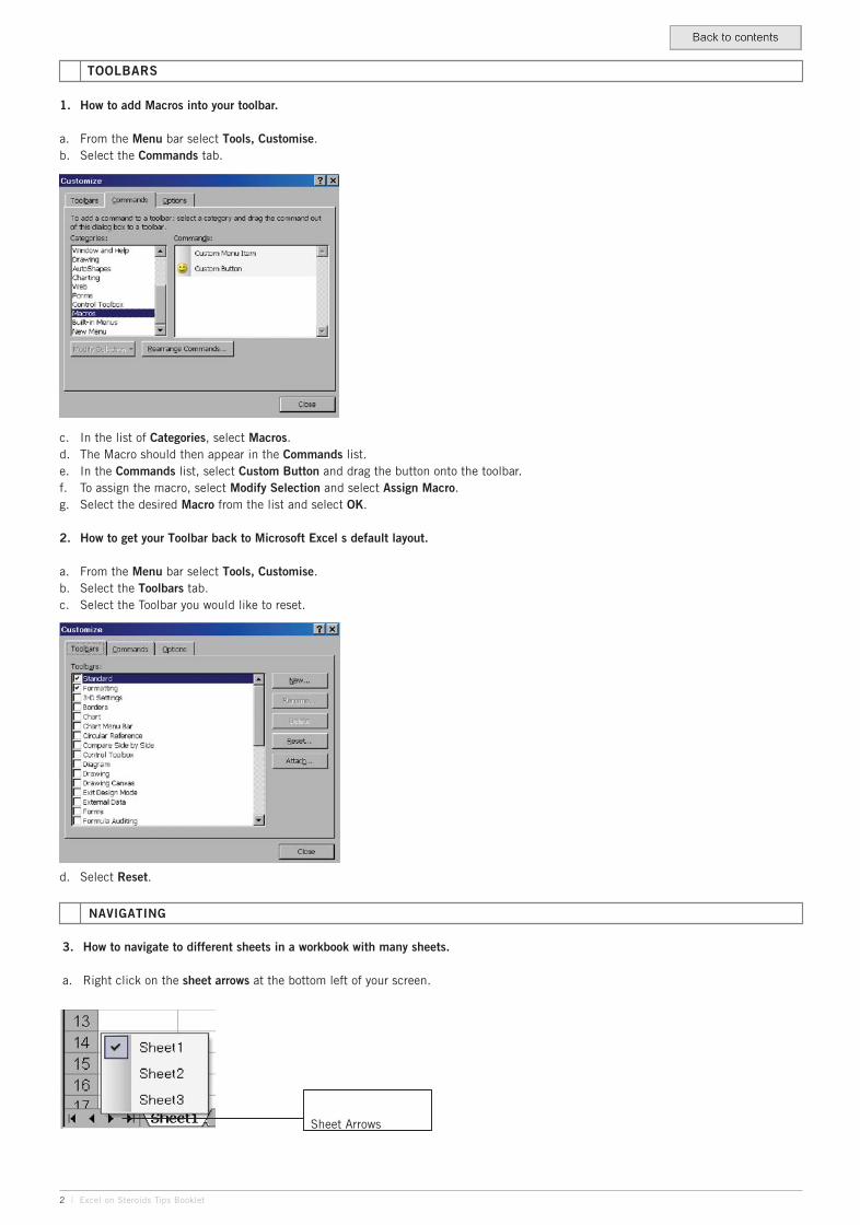
1. How to add Macros into your toolbar.

a. From the Menu bar select Tools, Customise.b. Select the Commands tab.

c. In the list of Categories, select Macros.d. The Macro should then appear in the Commands list.e. In the Commands list, select Custom Button and drag the button onto the toolbar.f. To assign the macro, select Modify Selection and select Assign Macro.g. Select the desired Macro from the list and select OK.

2. How to get your Toolbar back to Microsoft Excel s default layout.

a. From the Menu bar select Tools, Customise.b. Select the Toolbars tab.c. Select the Toolbar you would like to reset.

d. Select Reset.

Sheet Arrows

2 | Excel on Steroids Tips Booklet

NAVIGATING

3. How to navigate to different sheets in a workbook with many sheets.

a. Right click on the sheet arrows at the bottom left of your screen.

b. A list of the sheets in the file will be displayed.c. Left click on the sheet name you would like to navigate to.

4. There are two ways to quickly select a row

a. Select the row number.OR

b. Select any cell in that row and press Shift+Space bar.

PIVOTTABLE

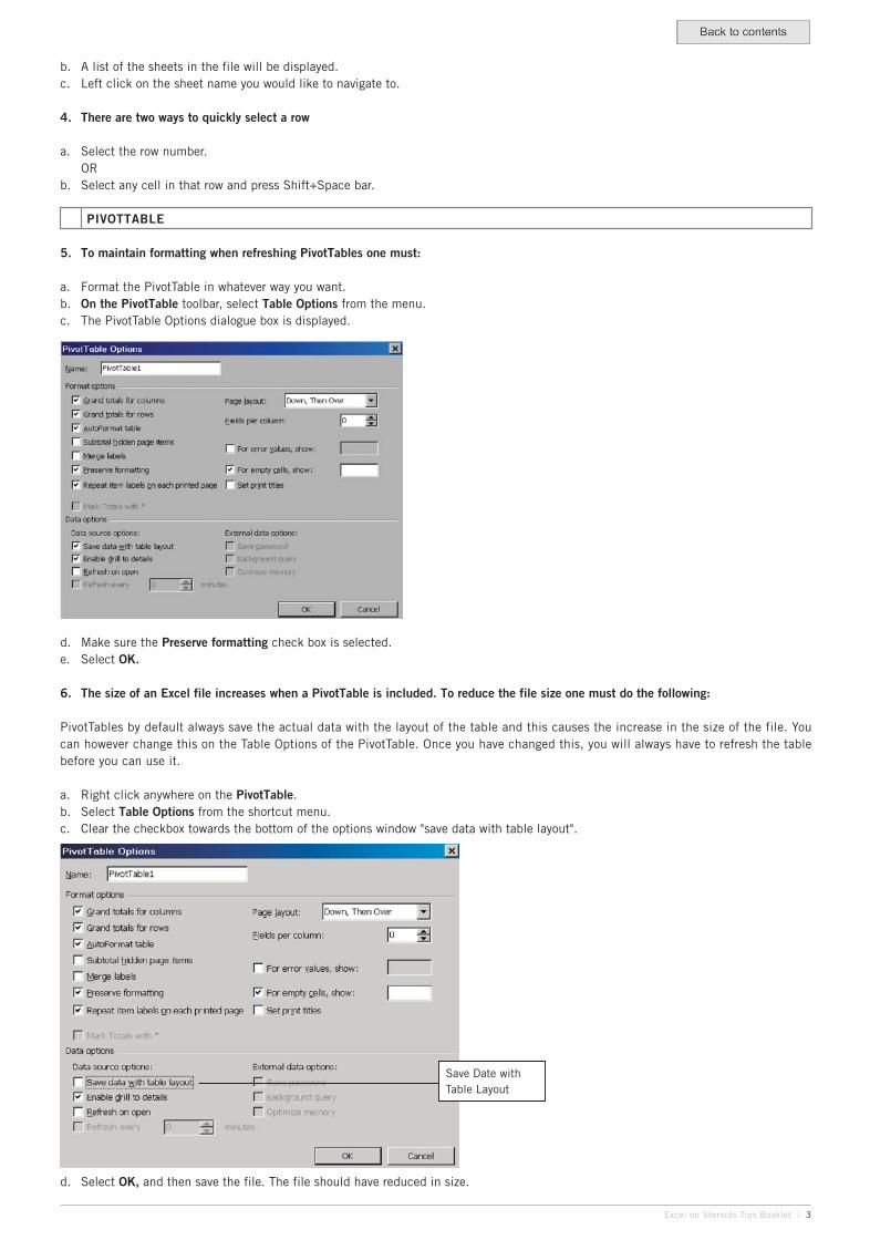
5. To maintain formatting when refreshing PivotTables one must:

a. Format the PivotTable in whatever way you want.b. On the PivotTable toolbar, select Table Options from the menu.c. The PivotTable Options dialogue box is displayed.

d. Make sure the Preserve formatting check box is selected.e. Select OK.

6. The size of an Excel file increases when a PivotTable is included. To reduce the file size one must do the following:

PivotTables by default always save the actual data with the layout of the table and this causes the increase in the size of the file. Youcan however change this on the Table Options of the PivotTable. Once you have changed this, you will always have to refresh the tablebefore you can use it.

a. Right click anywhere on the PivotTable.b. Select Table Options from the shortcut menu.c. Clear the checkbox towards the bottom of the options window "save data with table layout".

Save Date withTable Layout


d. Select OK, and then save the file. The file should have reduced in size.

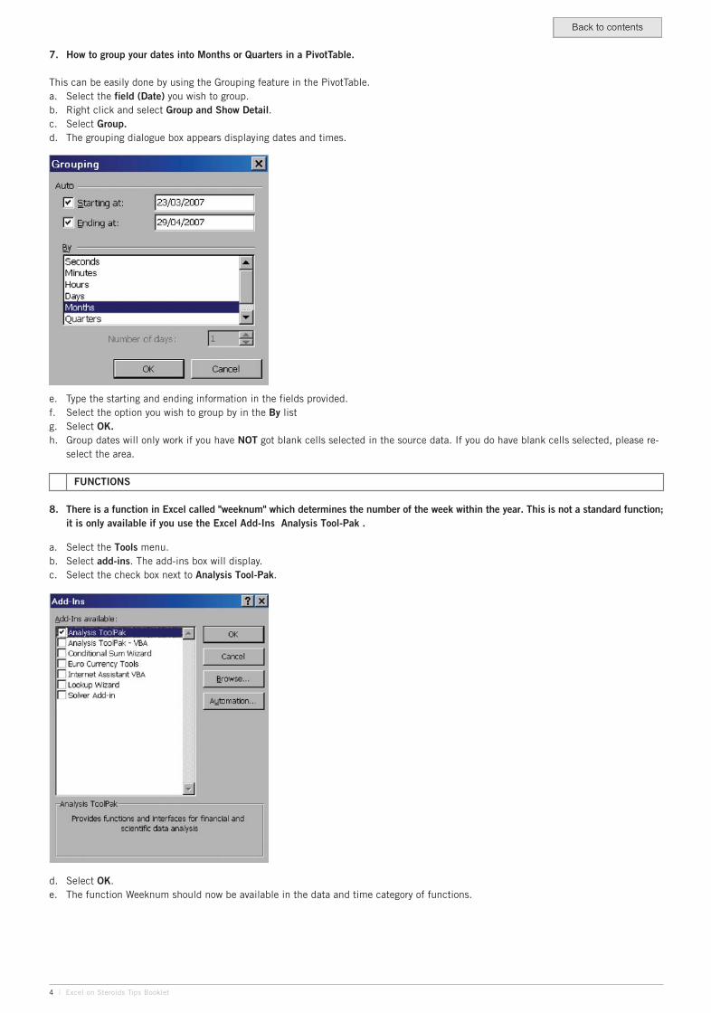
7. How to group your dates into Months or Quarters in a PivotTable.

This can be easily done by using the Grouping feature in the PivotTable.a. Select the field (Date) you wish to group.b. Right click and select Group and Show Detail.c. Select Group.d. The grouping dialogue box appears displaying dates and times.

e. Type the starting and ending information in the fields provided.f. Select the option you wish to group by in the By listg. Select OK.h. Group dates will only work if you have NOT got blank cells selected in the source data. If you do have blank cells selected, please re- select the area.

FUNCTIONS

8. There is a function in Excel called "weeknum" which determines the number of the week within the year. This is not a standard function; it is only available if you use the Excel Add-Ins Analysis Tool-Pak .

a. Select the Tools menu.b. Select add-ins. The add-ins box will display.c. Select the check box next to Analysis Tool-Pak.


d. Select OK.e. The function Weeknum should now be available in the data and time category of functions.

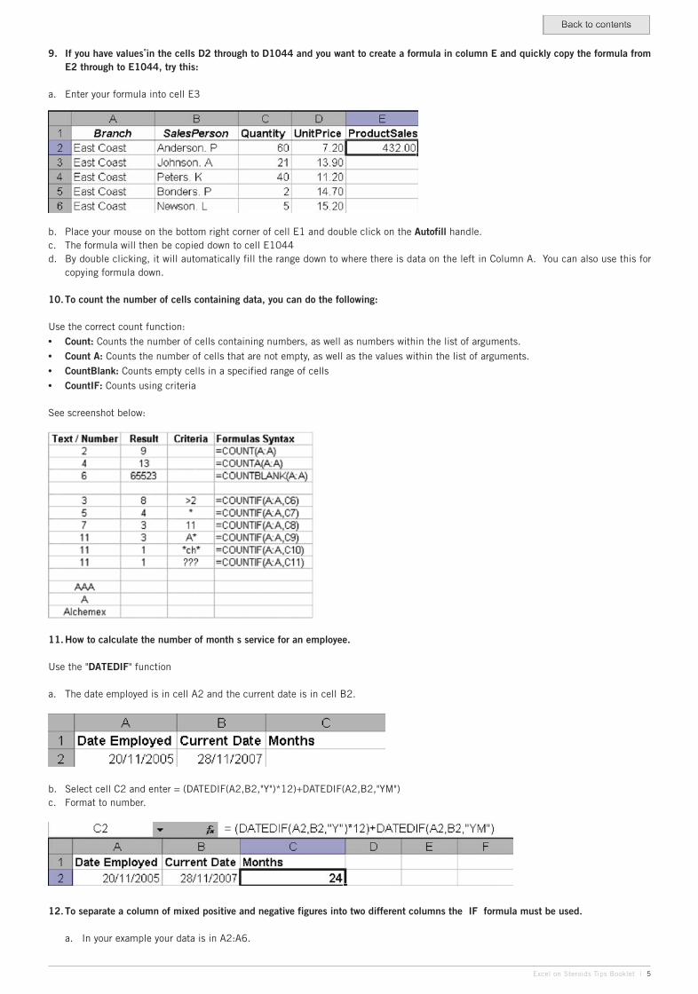
b. Place your mouse on the bottom right corner of cell E1 and double click on the Autofill handle.c. The formula will then be copied down to cell E1044d. By double clicking, it will automatically fill the range down to where there is data on the left in Column A. You can also use this for copying formula down.

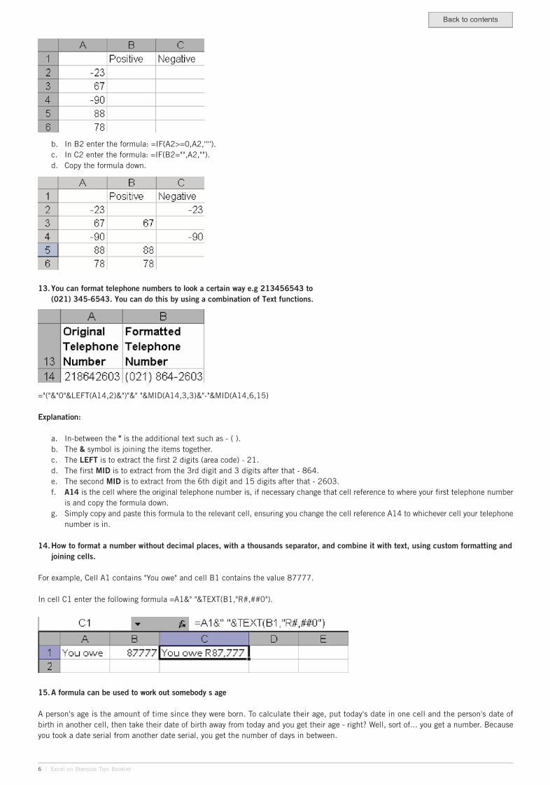
10.To count the number of cells containing data, you can do the following:

Use the correct count function:• Count: Counts the number of cells containing numbers, as well as numbers within the list of arguments.• Count A: Counts the number of cells that are not empty, as well as the values within the list of arguments.• CountBlank: Counts empty cells in a specified range of cells• CountIF: Counts using criteria

See screenshot below:

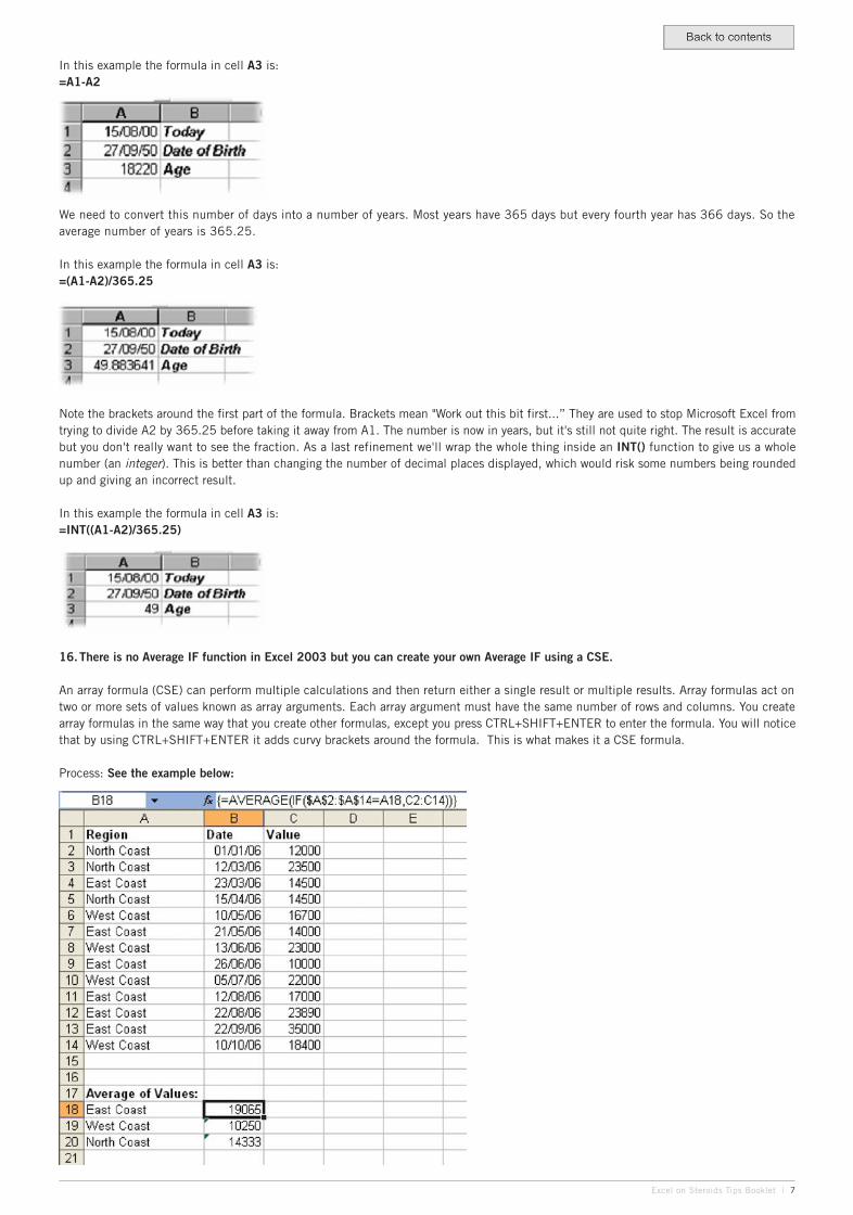
11.How to calculate the number of month s service for an employee.

Use the "DATEDIF" function

a. The date employed is in cell A2 and the current date is in cell B2.

b. Select cell C2 and enter = (DATEDIF(A2,B2,"Y")*12)+DATEDIF(A2,B2,"YM")c. Format to number.

12.To separate a column of mixed positive and negative figures into two different columns the IF formula must be used.

a. In your example your data is in A2:A6.

9. If you have values˚in the cells D2 through to D1044 and you want to create a formula in column E and quickly copy the formula from E2 through to E1044, try this:

a. Enter your formula into cell E3


13.You can format telephone numbers to look a certain way e.g 213456543 to (021) 345-6543. You can do this by using a combination of Text functions.

="("&"0"&LEFT(A14,2)&")"&" "&MID(A14,3,3)&"-"&MID(A14,6,15)

Explanation:

a. In-between the " is the additional text such as - ( ).b. The & symbol is joining the items together.c. The LEFT is to extract the first 2 digits (area code) - 21.d. The first MID is to extract from the 3rd digit and 3 digits after that - 864.e. The second MID is to extract from the 6th digit and 15 digits after that - 2603.f. A14 is the cell where the original telephone number is, if necessary change that cell reference to where your first telephone number

is and copy the formula down.g. Simply copy and paste this formula to the relevant cell, ensuring you change the cell reference A14 to whichever cell your telephone

number is in.

14.How to format a number without decimal places, with a thousands separator, and combine it with text, using custom formatting and joining cells.

For example, Cell A1 contains "You owe" and cell B1 contains the value 87777.

In cell C1 enter the following formula =A1&" "&TEXT(B1,"R#,##0").

15.A formula can be used to work out somebody s age

A person's age is the amount of time since they were born. To calculate their age, put today's date in one cell and the person's date ofbirth in another cell, then take their date of birth away from today and you get their age - right? Well, sort of... you get a number. Becauseyou took a date serial from another date serial, you get the number of days in between.


b. In B2 enter the formula: =IF(A2>=0,A2,'''').c. In C2 enter the formula: =IF(B2="",A2,"").d. Copy the formula down.

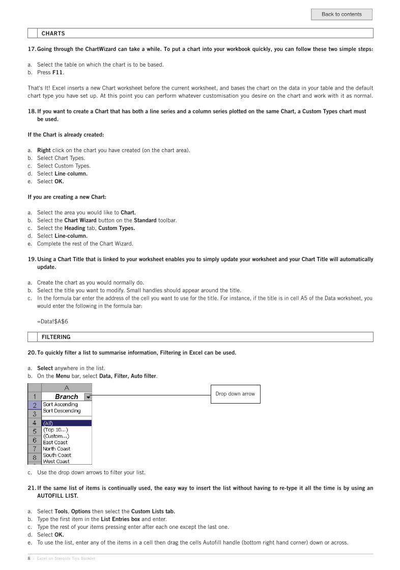
16.There is no Average IF function in Excel 2003 but you can create your own Average IF using a CSE.

An array formula (CSE) can perform multiple calculations and then return either a single result or multiple results. Array formulas act ontwo or more sets of values known as array arguments. Each array argument must have the same number of rows and columns. You createarray formulas in the same way that you create other formulas, except you press CTRL+SHIFT+ENTER to enter the formula. You will noticethat by using CTRL+SHIFT+ENTER it adds curvy brackets around the formula. This is what makes it a CSE formula.

Process: See the example below:


In this example the formula in cell A3 is:=A1-A2

We need to convert this number of days into a number of years. Most years have 365 days but every fourth year has 366 days. So theaverage number of years is 365.25.

In this example the formula in cell A3 is:=(A1-A2)/365.25

Note the brackets around the first part of the formula. Brackets mean "Work out this bit first...” They are used to stop Microsoft Excel fromtrying to divide A2 by 365.25 before taking it away from A1. The number is now in years, but it's still not quite right. The result is accuratebut you don't really want to see the fraction. As a last refinement we'll wrap the whole thing inside an INT() function to give us a wholenumber (an integer). This is better than changing the number of decimal places displayed, which would risk some numbers being roundedup and giving an incorrect result.

In this example the formula in cell A3 is:=INT((A1-A2)/365.25)

CHARTS

17.Going through the ChartWizard can take a while. To put a chart into your workbook quickly, you can follow these two simple steps:

a. Select the table on which the chart is to be based.b. Press F11.

That's It! Excel inserts a new Chart worksheet before the current worksheet, and bases the chart on the data in your table and the defaultchart type you have set up. At this point you can perform whatever customisation you desire on the chart and work with it as normal.

18. If you want to create a Chart that has both a line series and a column series plotted on the same Chart, a Custom Types chart must be used.

If the Chart is already created:

a. Right click on the chart you have created (on the chart area).b. Select Chart Types.c. Select Custom Types.d. Select Line-column.e. Select OK.

If you are creating a new Chart:

a. Select the area you would like to Chart.b. Select the Chart Wizard button on the Standard toolbar.c. Select the Heading tab, Custom Types.d. Select Line-column.e. Complete the rest of the Chart Wizard.

19.Using a Chart Title that is linked to your worksheet enables you to simply update your worksheet and your Chart Title will automatically update.

a. Create the chart as you would normally do.b. Select the title you want to modify. Small handles should appear around the title.c. In the formula bar enter the address of the cell you want to use for the title. For instance, if the title is in cell A5 of the Data worksheet, you would enter the following in the formula bar:

=Data!$A$6

FILTERING

20.To quickly filter a list to summarise information, Filtering in Excel can be used.

a. Select anywhere in the list.b. On the Menu bar, select Data, Filter, Auto filter.

c. Use the drop down arrows to filter your list.

21. If the same list of items is continually used, the easy way to insert the list without having to re-type it all the time is by using an AUTOFILL LIST.

a. Select Tools, Options then select the Custom Lists tab.b. Type the first item in the List Entries box and enter.c. Type the rest of your items pressing enter after each one except the last one.d. Select OK.e. To use the list, enter any of the items in a cell then drag the cells Autofill handle (bottom right hand corner) down or across.

Drop down arrow


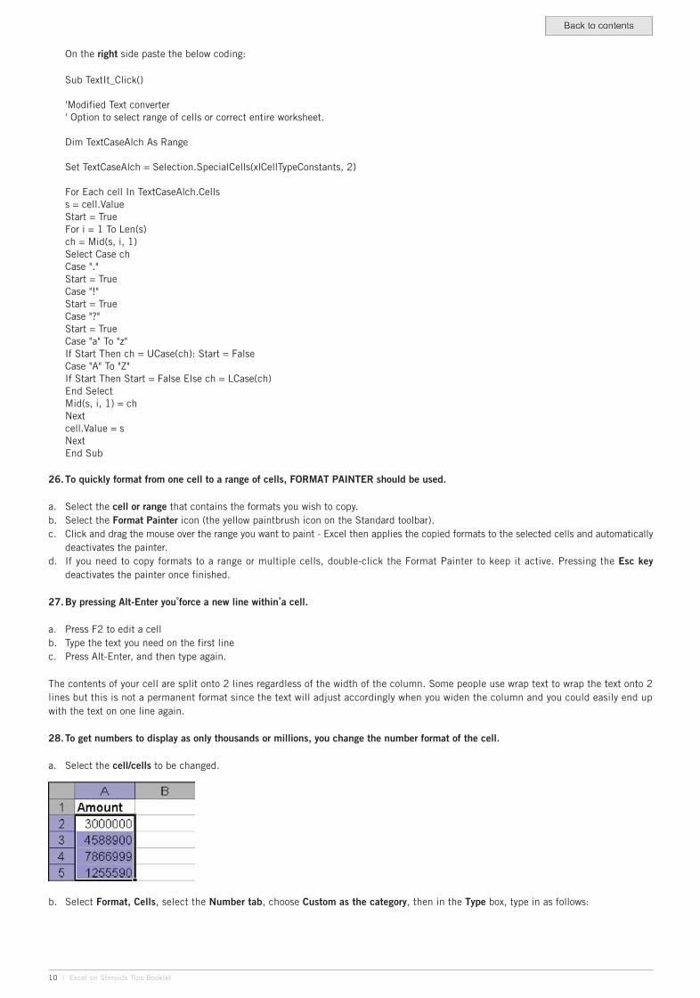
d. Select Finish.

25.To change a font type to Sentence case in Microsoft Excel, VB code must be inserted to the worksheet.

a. Open the required workbook.b. Right click on any worksheet.c. Select View Code.d. On the left, select This workbook.

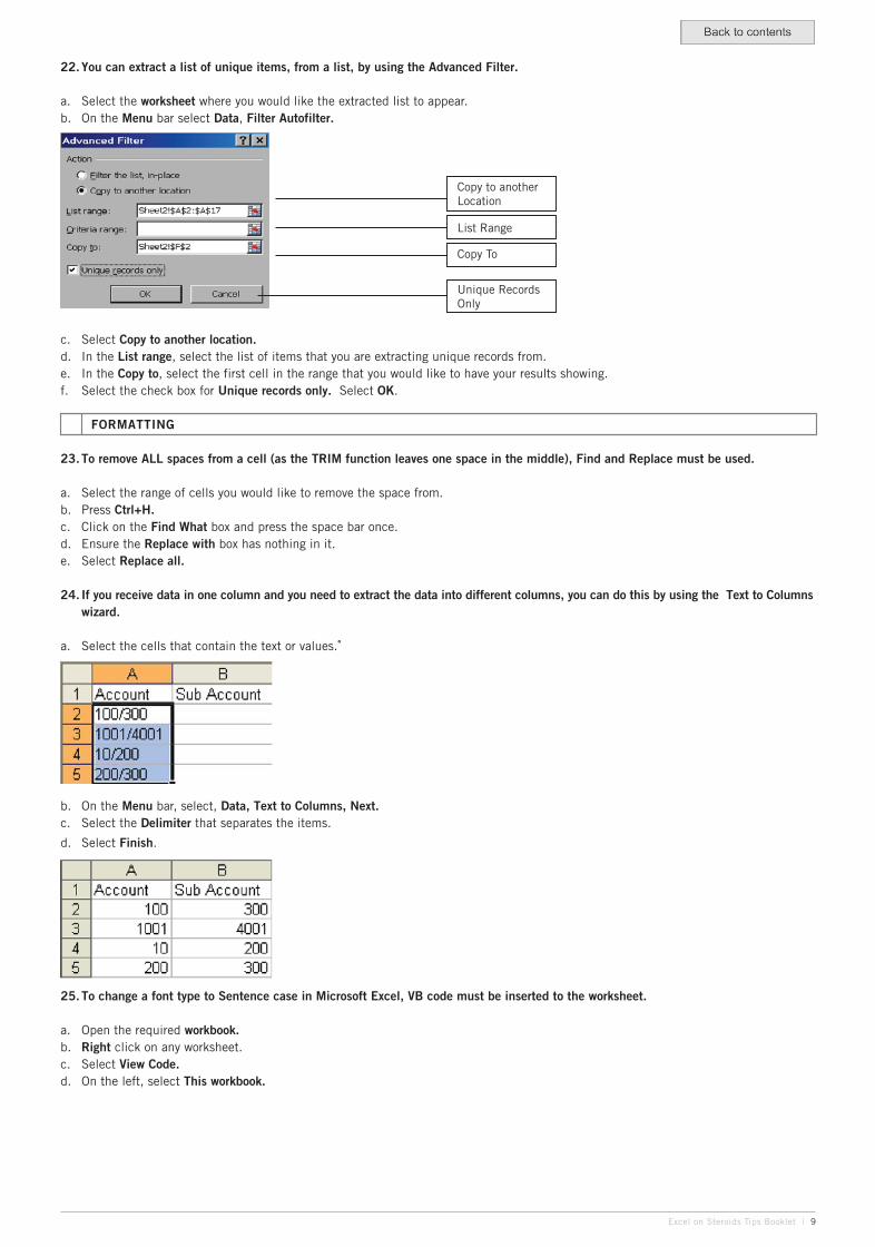
22.You can extract a list of unique items, from a list, by using the Advanced Filter.

a. Select the worksheet where you would like the extracted list to appear.b. On the Menu bar select Data, Filter Autofilter.

c. Select Copy to another location.d. In the List range, select the list of items that you are extracting unique records from.e. In the Copy to, select the first cell in the range that you would like to have your results showing.f. Select the check box for Unique records only. Select OK.

FORMATTING

23.To remove ALL spaces from a cell (as the TRIM function leaves one space in the middle), Find and Replace must be used.

a. Select the range of cells you would like to remove the space from.b. Press Ctrl+H.c. Click on the Find What box and press the space bar once.d. Ensure the Replace with box has nothing in it.e. Select Replace all.

24. If you receive data in one column and you need to extract the data into different columns, you can do this by using the Text to Columns wizard.

a. Select the cells that contain the text or values.˚

b. On the Menu bar, select, Data, Text to Columns, Next.c. Select the Delimiter that separates the items.

Copy to anotherLocation

List Range

Copy To

Unique RecordsOnly


On the right side paste the below coding:

Sub TextIt_Click()

'Modified Text converter' Option to select range of cells or correct entire worksheet.

Dim TextCaseAlch As Range

Set TextCaseAlch = Selection.SpecialCells(xlCellTypeConstants, 2)

For Each cell In TextCaseAlch.Cellss = cell.ValueStart = TrueFor i = 1 To Len(s)ch = Mid(s, i, 1)Select Case chCase "."Start = TrueCase "!"Start = TrueCase "?"Start = TrueCase "a" To "z"If Start Then ch = UCase(ch): Start = FalseCase "A" To "Z"If Start Then Start = False Else ch = LCase(ch)End SelectMid(s, i, 1) = chNextcell.Value = sNextEnd Sub

26.To quickly format from one cell to a range of cells, FORMAT PAINTER should be used.

a. Select the cell or range that contains the formats you wish to copy.b. Select the Format Painter icon (the yellow paintbrush icon on the Standard toolbar).c. Click and drag the mouse over the range you want to paint - Excel then applies the copied formats to the selected cells and automatically deactivates the painter.d. If you need to copy formats to a range or multiple cells, double-click the Format Painter to keep it active. Pressing the Esc key deactivates the painter once finished.

27.By pressing Alt-Enter you˚force a new line within˚a cell.

a. Press F2 to edit a cellb. Type the text you need on the first linec. Press Alt-Enter, and then type again.

The contents of your cell are split onto 2 lines regardless of the width of the column. Some people use wrap text to wrap the text onto 2lines but this is not a permanent format since the text will adjust accordingly when you widen the column and you could easily end upwith the text on one line again.

28.To get numbers to display as only thousands or millions, you change the number format of the cell.

a. Select the cell/cells to be changed.

b. Select Format, Cells, select the Number tab, choose Custom as the category, then in the Type box, type in as follows:


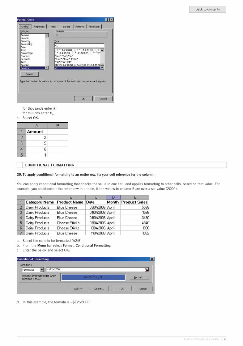
for thousands enter #,for millions enter #,,

c. Select OK.

CONDITIONAL FORMATTING

29.To apply conditional formatting to an entire row, fix your cell reference for the column.

You can apply conditional formatting that checks the value in one cell, and applies formatting to other cells, based on that value. Forexample, you could colour the entire row in a table, if the values in column E are over a set value (2000).

a. Select the cells to be formatted (A2:E).b. From the Menu bar select Format, Conditional Formatting.c. Enter the below and select OK:

d. In this example, the formula is =$E2>2000.


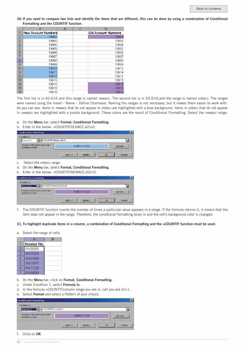
c. Select the oldacc range.d. On the Menu bar, select Format, Conditional Formatting.e. Enter in the below: =COUNTIF(NEWACC,D2)=0.

f. The COUNTIF function counts the number of times a particular value appears in a range. If the formula returns 0, it means that the item does not appear in the range. Therefore, the conditional formatting kicks in and the cell's background color is changed.

31.To highlight duplicate items in a column, a combination of Conditional Formatting and the =COUNTIF function must be used.

a. Select the range of cells.

b. On the Menu bar, click on Format, Conditional Formatting.c. Under Condition 1, select Formula Is.d. In the formula =COUNTIF(column range you are in, cell you are in)>1.e. Select Format and select a Pattern of your choice.

f. Click on OK.

The first list is in A2:A16 and this range is named newacc. The second list is in D2:D16,and the range is named oldacc. The rangeswere named using the Insert - Name – Define Command. Naming the ranges is not necessary, but it makes them easier to work with.As you can see, items in newacc that do not appear in oldacc are highlighted with a blue background. Items in oldacc that do not appearin newacc are highlighted with a purple background. These colors are the result of Conditional Formatting. Select the newacc range.

a. On the Menu bar, select Format, Conditional Formatting.b. Enter in the below: =COUNTIF(OLDACC,A2)=0.


30. If you need to compare two lists and identify the items that are different, this can be done by using a combination of Conditional Formatting and the COUNTIF function.

SHORTCUTS

32. If you have a number of open workbooks and you want to close them all, this can be done by using the Shift key.

a. Hold down the Shift key as you select File on the Menu bar.b. You will notice that there is a Close All option.c. Choose this, and all your workbooks are closed.d. You will, of course, be prompted to save changes on each open workbook, if necessary.

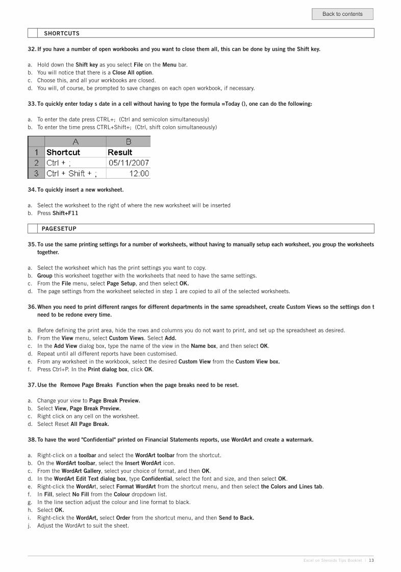
33.To quickly enter today s date in a cell without having to type the formula =Today (), one can do the following:

a. To enter the date press CTRL+; (Ctrl and semicolon simultaneously)b. To enter the time press CTRL+Shift+; (Ctrl, shift colon simultaneously)

34.To quickly insert a new worksheet.

a. Select the worksheet to the right of where the new worksheet will be insertedb. Press Shift+F11

PAGESETUP

35.To use the same printing settings for a number of worksheets, without having to manually setup each worksheet, you group the worksheets together.

a. Select the worksheet which has the print settings you want to copy.b. Group this worksheet together with the worksheets that need to have the same settings.c. From the File menu, select Page Setup, and then select OK.d. The page settings from the worksheet selected in step 1 are copied to all of the selected worksheets.

36.When you need to print different ranges for different departments in the same spreadsheet, create Custom Views so the settings don t need to be redone every time.

a. Before defining the print area, hide the rows and columns you do not want to print, and set up the spreadsheet as desired.b. From the View menu, select Custom Views. Select Add.c. In the Add View dialog box, type the name of the view in the Name box, and then select OK.d. Repeat until all different reports have been customised.e. From any worksheet in the workbook, select the desired Custom View from the Custom View box.f. Press Ctrl+P. In the Print dialog box, click OK.

37.Use the Remove Page Breaks Function when the page breaks need to be reset.

a. Change your view to Page Break Preview.b. Select View, Page Break Preview.c. Right click on any cell on the worksheet.d. Select Reset All Page Break.

38.To have the word "Confidential" printed on Financial Statements reports, use WordArt and create a watermark.

a. Right-click on a toolbar and select the WordArt toolbar from the shortcut.b. On the WordArt toolbar, select the Insert WordArt icon.c. From the WordArt Gallery, select your choice of format, and then OK.d. In the WordArt Edit Text dialog box, type Confidential, select the font and size, and then select OK.e. Right-click the WordArt, select Format WordArt from the shortcut menu, and then select the Colors and Lines tab.f. In Fill, select No Fill from the Colour dropdown list.g. In the line section adjust the colour and line format to black.h. Select OK.i. Right-click the WordArt, select Order from the shortcut menu, and then Send to Back.j. Adjust the WordArt to suit the sheet.


39.To apply the same Header and Footer to some of the worksheets on a workbook, Group (select) the required sheets together andthen create the Header and Footer .

a. Select the worksheets - if the worksheets are adjacent to one another, select the sheet tab of the first sheet in the range, hold the Shift key then select the last sheet in the range.b. If the sheets are not adjacent to one another then select the first sheet, hold the Ctrl key, select all other sheet tabs of the sheets you wish to apply the header and footer to.c. Select File, Page Setup, Header and Footer.d. Apply the header and footer.e. To ungroup the sheets, hold the shift key then click on the first sheet tab within the group.

40.When you click on a cell which contains a very long formula, it often takes up more than 2 lines of text in the formula bar and it hides the first rows of your spreadsheet. To overcome this, insert a blank row at the top of the worksheet and increase the row height.

a. To insert a blank row – Right click on Row 1, then select Insert, Rows.b. Increase the row height of the new row by selecting, Format, Row, Height, then type in a high number e.g.50

41.To display two worksheets in a workbook on the screen, at the same time, in order to make it easier to complete work - do the following:

a. Open the workbook; activate one of the worksheets you need to display.b. Select Window, New Window.c. The workbook will open a second time. In this workbook activate the second sheet you need to display.d. Now select Window, Arrange Windows.e. Tick the check box "Windows of active workbook", choose the display you want e.g. tiled, vertical etc.f. Select OK.

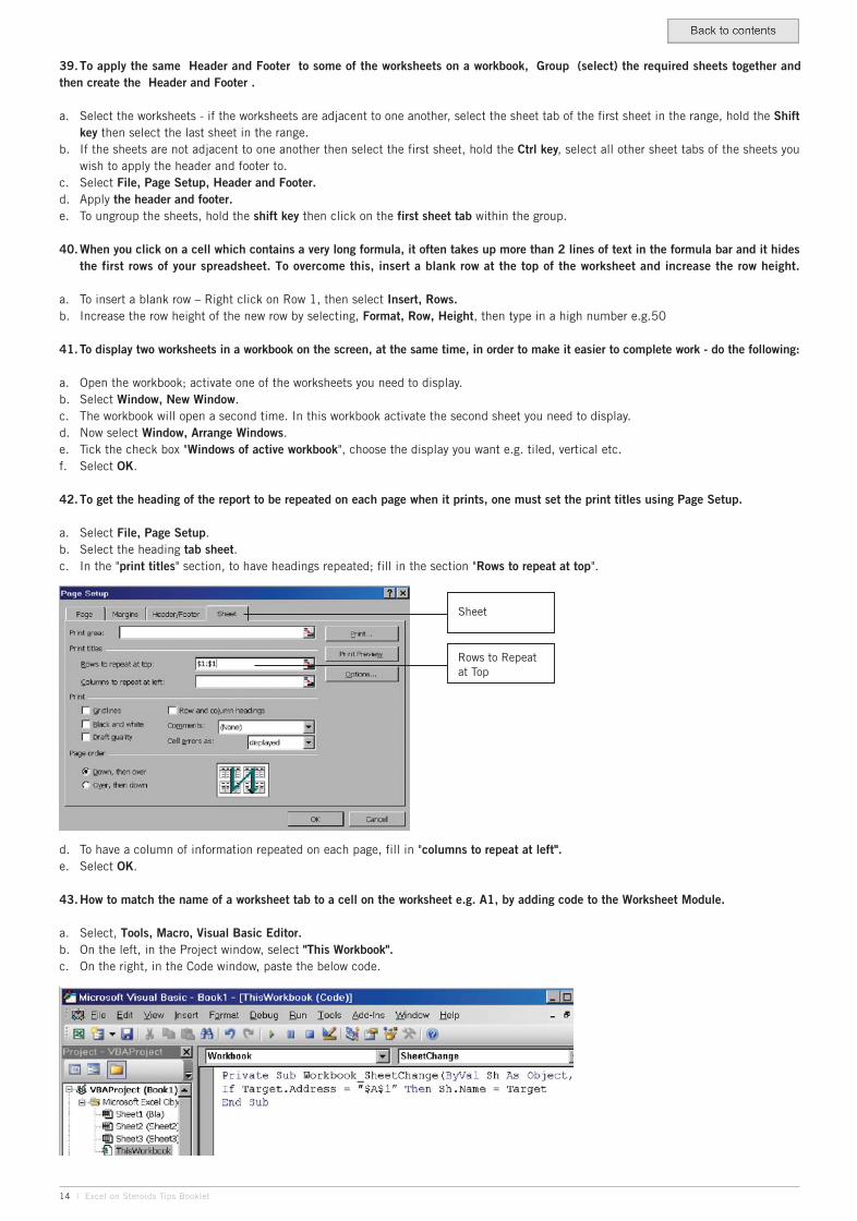
42.To get the heading of the report to be repeated on each page when it prints, one must set the print titles using Page Setup.

a. Select File, Page Setup.b. Select the heading tab sheet.c. In the "print titles" section, to have headings repeated; fill in the section "Rows to repeat at top".

d. To have a column of information repeated on each page, fill in "columns to repeat at left".e. Select OK.

43.How to match the name of a worksheet tab to a cell on the worksheet e.g. A1, by adding code to the Worksheet Module.

a. Select, Tools, Macro, Visual Basic Editor.b. On the left, in the Project window, select "This Workbook".c. On the right, in the Code window, paste the below code.

Sheet

Rows to Repeatat Top


Private Sub Workshop_SheetChange(ByVal Sh As Object, ByVal Target As Range)If Target.Address = "$A$1" Then Sh.Name = TargetEnd Sub

d. Select File, Close and Return to Microsoft Excel.

HYPERLINKS

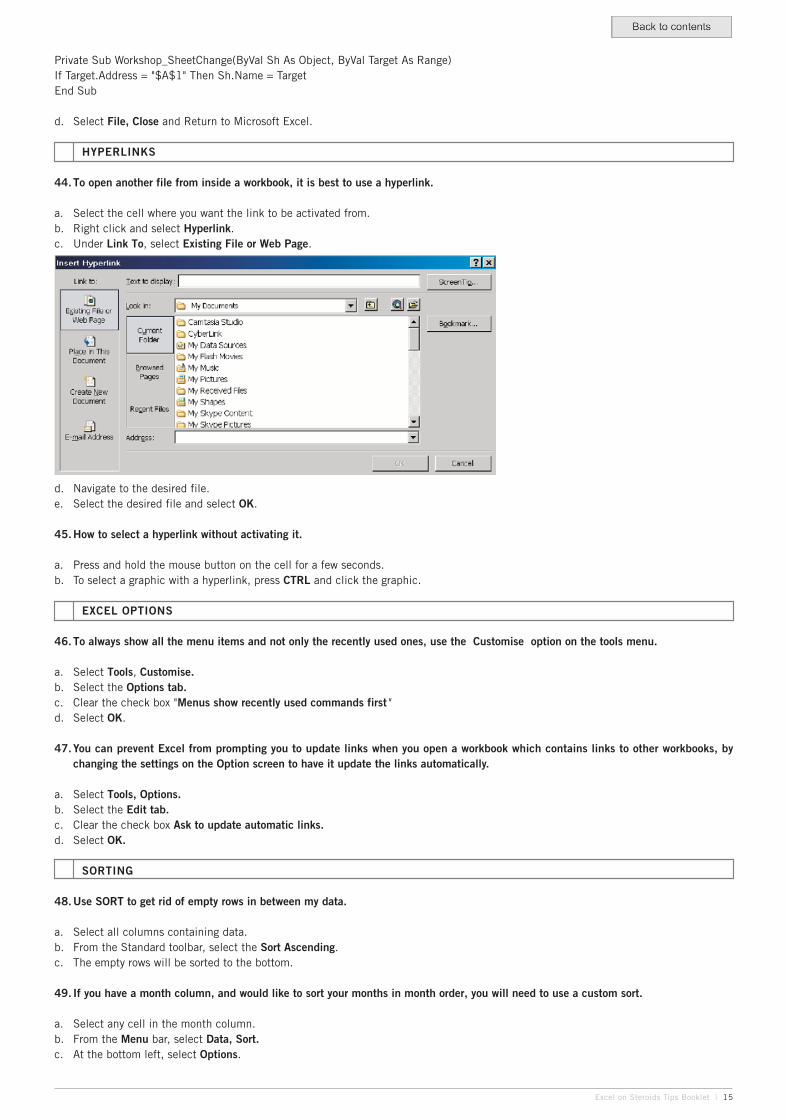
44.To open another file from inside a workbook, it is best to use a hyperlink.

a. Select the cell where you want the link to be activated from.b. Right click and select Hyperlink.c. Under Link To, select Existing File or Web Page.

d. Navigate to the desired file.e. Select the desired file and select OK.

45.How to select a hyperlink without activating it.

a. Press and hold the mouse button on the cell for a few seconds.b. To select a graphic with a hyperlink, press CTRL and click the graphic.

EXCEL OPTIONS

46.To always show all the menu items and not only the recently used ones, use the Customise option on the tools menu.

a. Select Tools, Customise.b. Select the Options tab.c. Clear the check box "Menus show recently used commands first"d. Select OK.

47.You can prevent Excel from prompting you to update links when you open a workbook which contains links to other workbooks, by changing the settings on the Option screen to have it update the links automatically.

a. Select Tools, Options.b. Select the Edit tab.c. Clear the check box Ask to update automatic links.d. Select OK.

SORTING

48.Use SORT to get rid of empty rows in between my data.

a. Select all columns containing data.b. From the Standard toolbar, select the Sort Ascending.c. The empty rows will be sorted to the bottom.

49. If you have a month column, and would like to sort your months in month order, you will need to use a custom sort.

a. Select any cell in the month column.b. From the Menu bar, select Data, Sort.c. At the bottom left, select Options.


d. Select the months as your First key sort order.e. Select OK.

SUBTOTALS

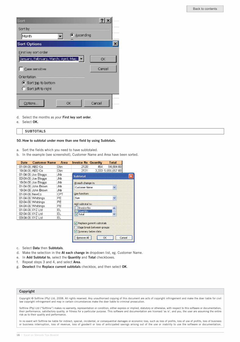
50.How to subtotal under more than one field by using Subtotals.

a. Sort the fields which you need to have subtotaled.b. In the example (see screenshot), Customer Name and Area have been sorted.

c. Select Data then Subtotals.d. Make the selection in the At each change in dropdown list, eg. Customer Name.e. In Add Subtotal to, select the Quantity and Total checkboxes.f. Repeat steps 3 and 4, and select Area.g. Deselect the Replace current subtotals checkbox, and then select OK.


Copyright

Copyright © Softline (Pty) Ltd, 2008. All rights reserved. Any unauthorised copying of this document are acts of copyright infringement and make the doer liable for civillaw copyright infringement and may in certain circumstances make the doer liable to criminal prosecution.

Softline (Pty) Ltd (“Softline”) makes no warranty, representation or condition, either express or implied, statutory or otherwise, with respect to this software or documentation,their performance, satisfactory quality, or fitness for a particular purpose. This software and documentation are licensed ‘as is’, and you, the user are assuming the entirerisk as to their quality and performance.

In no event will Softline be liable for indirect, special, incidental, or consequential damages or economic loss, such as loss of profits, loss of use of profits, loss of businessor business interruption, loss of revenue, loss of goodwill or loss of anticipated savings arising out of the use or inability to use the software or documentation.

Documents

Excel on Steroids Tips Booklet - Ningapi.ning.com/files/bKgApL8YprvhAANHDOVBfRiariL0M0... · Excel on Steroids Tips Booklet | 1 ... Navigating pg 2 PivotTable pg 3 Functions pg 4