Excel Advanced 07 - GCU · 2019-01-30 · Vertical LOOKUP (VLOOKUP) ... Excel is a spreadsheet application used for storing number and text data and for performing numerical calculations

Excel Advanced Using a Computer for Numerical Calculations

Microsoft Office 2007

MMiiccrroossoofftt EExxcceell AAddvvaanncceedd

2 © ICT Skills Glasgow Caledonian University

Contents: When/If Things Go Wrong .................................................................................................... 4

To rectify problems such as a wrongly entered menu command: ............................... 4

To close a window/dialogue box: .................................................................................. 4

Using Help ......................................................................................................................... 4

What is Excel? .................................................................................................................... 5

What is Data? .................................................................................................................... 6

Qualitative or Categorical Data (Nominal, Ordinal) ...................................................... 6

Quantitative Data (Discreet,Continuous) ...................................................................... 6

Starting Excel and Entering Data ........................................................................................... 7

Saving a Spreadsheet ........................................................................................................ 7

Closing a Spreadsheet ....................................................................................................... 7

Opening a Spreadsheet ..................................................................................................... 8

Editing and Inserting Data ............................................................................................. 8

Conditional Formatting ................................................................................................. 8

Naming Sheets ............................................................................................................... 9

Sorting data ..................................................................................................................... 10

Filtering Data ................................................................................................................... 10

The Filter Command .................................................................................................... 11

Using the Custom AutoFilter ....................................................................................... 11

Comparison Operators ................................................................................................ 13

Parsing Data .................................................................................................................... 13

Functions and Formula ........................................................................................................ 15

Cell Referencing ........................................................................................................... 15

Sum Function/Formula .................................................................................................... 16

Average Function/Formula ............................................................................................. 16

Conditional (Logical) Function/Formula .......................................................................... 17

IF .................................................................................................................................. 17

COUNTIF ...................................................................................................................... 18

LOOK UP Function ........................................................................................................... 20

Vertical LOOKUP (VLOOKUP) ....................................................................................... 20

VLOOKUP Errors .......................................................................................................... 22

SUBTOTALS ...................................................................................................................... 22


© ICT Skills 3 Glasgow Caledonian University

Charts and Graphs ............................................................................................................... 24

Chart Types and Uses ...................................................................................................... 24

Column/Bar Charts ...................................................................................................... 24

Line Charts ................................................................................................................... 24

Pie Charts ..................................................................................................................... 24

XY Scatter Charts ......................................................................................................... 24

Creating a Chart ............................................................................................................... 25

Moving and Resizing a Chart ........................................................................................... 26

Inserting/Modifying a Chart Title .................................................................................... 27

Formatting a Series Title and Axis Labels ........................................................................ 28

Modifying Charts ............................................................................................................. 29

Formatting Charts ............................................................................................................ 31

PivotTables .......................................................................................................................... 32

These notes are designed for you to work through at your own pace.

These notes do not explain every feature of the application therefore you are expected to make use of the Help facility.

If you have any comments or queries, please contact the ICT Skills Unit:

Room: M015, ground floor, George Moore building

Email: [email protected]

Tel: 0141 273 1373



When you have completed these notes you should be able to:

• Format Data

• Sort Data

• Filter Data

• Parse Data

• Use Excel’s Function

• Create Charts

• Format Charts

• Insert PivotTables

The following notes will introduce some of the features and functionality within Excel. They do not cover all aspects of the application. This booklet is aimed at students who are already familiar with the content of the Spreadsheets booklet.

When/If Things Go Wrong Before you start using Excel, remember that when/if an error occurs try the following to rectify the situation:

To rectify problems such as a wrongly entered menu command:

Use the Undo option by clicking on the Undo command in the Quick Access Toolbar.

To close a window/dialogue box:

Click on the close command at the top right‐hand side of the window or dialogue box.

If all else fails, exit from Excel (select the Office Button and click on the Exit Excel option) and start again.

Using Help

If there is a command or feature of Excel you would like to use but do not know how to, use the Help facility within the application. This provides instructions and advice on using all of the features of the software. To use Help, simply click on the Help command and then click on one of the options displayed or type in a help phrase. You will then be given a list of phrases which are nearest matches to your question. Select the topic you require from the list.

Note: This icon denotes important information – read it carefully.

Tasks This icon denotes a task which should be carried out to help you gain the skills required.



What is Excel?

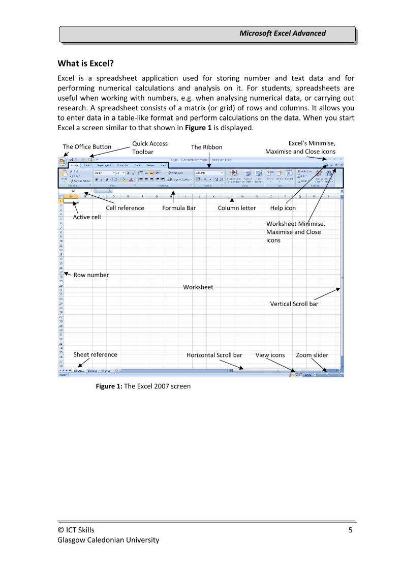
Excel is a spreadsheet application used for storing number and text data and for performing numerical calculations and analysis on it. For students, spreadsheets are useful when working with numbers, e.g. when analysing numerical data, or carrying out research. A spreadsheet consists of a matrix (or grid) of rows and columns. It allows you to enter data in a table‐like format and perform calculations on the data. When you start Excel a screen similar to that shown in Figure 1 is displayed.

Figure 1: The Excel 2007 screen

Quick Access Toolbar

Cell reference Formula Bar Column letter

The RibbonThe Office Button Excel’s Minimise, Maximise and Close icons

Worksheet Minimise, Maximise and Close icons

Help icon Active cell

Row number

Sheet reference

Worksheet

Zoom slider View icons Horizontal Scroll bar

Vertical Scroll bar



What is Data?

Data is essentially information and can be either quantitative or qualitative.

Qualitative or Categorical Data (Nominal, Ordinal)

This data is non numeric and can be gathered from questionnaires, interviews and written documentation. The data are merely labels or categories. The two main types are:

Nominal Data: The type of categorical data in which objects fall into unordered categories. Some examples are: gender, hair colour, smoking status and so on.

Ordinal Data: The type of data in which the order is important. This data can be ranked or have a value in a scale. In a questionnaire you could be asked to rate your response from 1 ‐5 with 1 being the lowest and 5 being the highest.

Quantitative Data (Discreet,Continuous)

This data is numerical data which can be measured based on some quantitative trait on a scale and can be analysed statistically. The results are set of numbers. The two main types are:

Discreet Data: This data has values which are distinct and separate. Discreet data could be the number of students in a class.

Continuous Data: This data can be counted, ordered or measured. Continuous data could be your height, weight etc.

There are 3 basic types of data which can be entered into cells:

(a) Numbers – in Excel a number can only contain the following characters: 0 1 2…9 + ‐ ( ) , £ . %

Note: When entered, numbers are right‐aligned i.e. they are aligned to the right of the cell. The , £ . % characters are left aligned unless they are accompanied by numbers.

(b) Text or labels – text can include any character from the keyboard and is used for entering sheet, row and column headings and descriptions.

Note: When entered, text is left‐aligned i.e. it is aligned to the left of the cell.

(c) Formulae – these allow calculations to be performed based on the values stored in the cells. Any formula must be prefixed by the ‘=’ sign e.g. if you were to add the contents of the two cells B3 and C4 together, the formula would be entered as =B3+C4. Excel provides some standard formulae e.g. SUM, Average, STDEV, etc. called functions which are entered using menus and Wizards (see later for instructions on how to use them). When a formula is entered in a cell, the result of the calculation is displayed on the sheet, while the formula itself is displayed in the Formula Bar.



Starting Excel and Entering Data Excel is opened from the Start menu (displayed on the Taskbar at the bottom of the screen). After clicking the Start button, select Programs then Microsoft Office then Microsoft Office Excel 2007. This should open and display a blank worksheet ready for data to be entered, see Figure 1 below.

To enter data, select the appropriate cell (using the mouse or arrow keys), and type the data. Then press the ENTER key, or any arrow key (to move to a new column or row), or click on the in the Formula Bar (which appears once you start typing into a cell).

Saving a Spreadsheet

To save a spreadsheet for the first time, click the Office Button and choose Save As. The Save As dialogue box will appear prompting you to choose a file name and location (i.e. the drive and folder).

Further saves will use the same file name and ‘overwrite’ the previously saved version. To re‐save a document simply click on the Save command from the Quick Access Toolbar, see Figure 2 below.

Figure 2: The Save command in the Quick Access Toolbar

Closing a Spreadsheet

After saving a spreadsheet, it will still be displayed on the screen. To close it select the Office Button and choose Close. This closes the spreadsheet but not Excel. To close Excel, select the Office Button and choose Exit Excel, or click on the close command at the top right hand side of the application .

Task 1

Open Excel and enter the following data into a new spreadsheet:

Adjust column widths if necessary. If you are unsure of how to do this please refer to the Spreadsheets booklet.



Opening a Spreadsheet

To open a previously saved spreadsheet, select the Office Button and choose Open. Select the name and location (i.e. the drive/folder) of the stored file and click on the Open button.

Editing and Inserting Data

The contents or the appearance of a spreadsheet can be changed using a few simple commands. To edit the contents of a spreadsheet move to and select the appropriate cell, either by double clicking in it or single click it and go to the Formula Bar to edit as appropriate. Data can be inserted by clicking on, or moving to, the appropriate cell and typing the data (see Spreadsheets booklet if unsure).

Conditional Formatting

In Excel data can be difficult to immediately understand. Conditional formatting allows you to apply formatting which will change the appearance of one or more cells or the data within a cell if it meets specified criteria. This will make the data stand out visually and enables patterns and trends to be identified. To apply conditional formatting select the cell or range of cells you wish to apply formatting to. Then from the Home tab select the Style group and Conditional Formatting command. A Conditional Formatting drop‐down menu will appear with options for formatting, see Figure 3 below.

Task 3

Make the following changes to your spreadsheet:

James Brown – should read John Brown; Gordon Smith – date of birth should read 29/09/1980

Add the following to the spreadsheet beneath the existing data:

Task 2

Save the spreadsheet to your user workspace (H: drive), or USB drive calling it ICT Student Data.

Close the ICT Student Data spreadsheet.



Figure 3: Conditional Formatting menu

From the drop‐down menu choose the option you wish. For example if the pass mark for the ICT Skills module was 32 out of 40 and we wished to see all pass marks in green and those below in red you can apply conditional formatting to do this. Firstly highlight the cells in the Mark column. Click the Conditional Formatting command and a drop‐down menu will appear. Choose the Highlight Cell Rules option, a further menu will appear, choose the Between option. The Between dialogue box will appear. Type the values in the fields and choose the conditional formatting you wish to apply. If you do not see the colours you wish choose Custom Format… from the drop‐down menu. Click OK. Now apply conditional formatting to the cells so that any cells containing a value below 32 appear in red.

Note: To remove or modify a conditional formatting select the data which has conditional formatting applied and from the Home tab, Styles group, click on the Conditional Formatting command. From the drop‐down menu that appears choose Manage Rules…. You will then see all rules applied to the data and you can choose to modify or remove any of the rules.

Naming Sheets

Sheets are named by default as Sheet1, Sheet2 and Sheet3. To change the name of a sheet, simply double click on the sheet tab at the bottom of the screen (it should then be highlighted) and then type a new name.

Task 5

Change the name of Sheet1 to ICT Data 2008. Re‐save the spreadsheet.

Task 4

Open the ICT Student Data spreadsheet. Apply conditional formatting to show the text orange if a student has passed and blue if they have failed.

Conditional Formatting command drop‐down menu and further options



Column Sort drop‐down list

Header Row selector

Sorting data

Data in rows or columns can be sorted either alphabetically or numerically, in ascending or descending order. To sort data, firstly select all cells that contain the data to be sorted (not just the column or the row data has to be ordered by), then from the Data tab, Sort & Filter group click on the Sort command, see Figure 4 below.

Figure 4: Sort & Filter group in the Data tab.

Figure 5: Sort dialogue box.

The Sort dialogue box will appear. You can specify whether or not the data you have selected has a header row by checking the option, see Figure 5 above. Choose a column heading to sort by from the Sort drop‐down menu, then values and sort order from the respective drop‐down menus. When you are happy with the options selected, click OK to perform the sort.

Note: When performing a sort, you must select all data to be sorted, e.g. select numbers and formulae as well as labels if sorting alphabetically – for example if you have student information in various columns, but wish to sort by Matric No you need to ensure that all columns are highlighted, not just Column A. This way the correct details will remain with the correct student.

Note: Remember if the data has not been sorted correctly, you can use the Undo option to get the data back to its original form and try again.

Filtering Data

When working in Excel you can choose to filter data to create a data subset which displays only information which meets criteria specified by you. The data in the other rows will be hidden. You can filter by text, number, date, etc. For example if you wished to show only students who had passed the ICT Skills module you could filter this information into a subset. After data has been filtered it can be copied, edited, charted etc. There are two main tools available for filtering data these are, the Filter Command and the Custom AutoFilter.

Task 6

Sort the data alphabetically by Course Code. Re‐save the ICT Student Data spreadsheet.



The Filter Command

Select a cell and then from the Data tab select the Filter command from the Sort and Filter group (see Figure 6 below).

Figure 6: The Data tab showing the Sort & Filter group and the Filter command

Filter arrows will appear at the top of the columns. Choose which column you wish to filter by and click the Filter arrow . A drop‐down menu will appear giving all of the sorting and filtering options (see Figure 7 below). The sorting options are at the top of the drop‐down menu and the filtering ones are at the bottom. By default all of the options in the filtering section will be selected, that is they will have a tick in the check box. To choose your own filter criteria, remove the default settings by clicking on the Select All check box at the top. All of the ticks will be removed from the check boxes. Then choose the criteria you wish to filter by. You could, for example, choose to display only those students who are in level one.

Note: You can also filter by using the Sort and Filter command in the Editing group of the Home tab.

Figure 7: Filter arrows

Using the Custom AutoFilter

You can also specify or customise the values you wish to filter by. To do this, select a cell in your workbook, then from the Data tab, Sort and Filter group choose the Filter

Task 7

Use the Filter command to filter the data to show a subset containing only students who have passed the ICT Skills module.

Data tab

Filter arrows

Drop‐down menu with options

Filtering options and the Select All option

Filter commandSort & Filter group



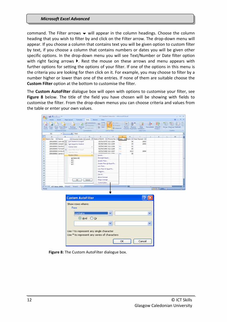
command. The Filter arrows will appear in the column headings. Choose the column heading that you wish to filter by and click on the Filter arrow. The drop‐down menu will appear. If you choose a column that contains text you will be given option to custom filter by text, if you choose a column that contains numbers or dates you will be given other specific options. In the drop‐down menu you will see Text/Number or Date filter option with right facing arrows . Rest the mouse on these arrows and menu appears with further options for setting the options of your filter. If one of the options in this menu is the criteria you are looking for then click on it. For example, you may choose to filter by a number higher or lower than one of the entries. If none of them are suitable choose the Custom Filter option at the bottom to customise the filter.

The Custom AutoFilter dialogue box will open with options to customise your filter, see Figure 8 below. The title of the field you have chosen will be showing with fields to customise the filter. From the drop‐down menus you can choose criteria and values from the table or enter your own values.

Figure 8: The Custom AutoFilter dialogue box.



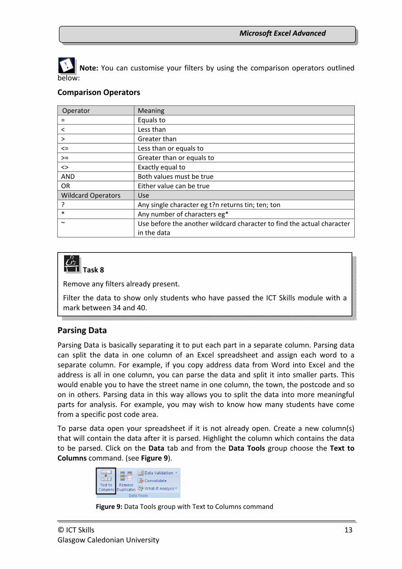
Note: You can customise your filters by using the comparison operators outlined below:

Comparison Operators

Operator Meaning = Equals to < Less than > Greater than <= Less than or equals to >= Greater than or equals to <> Exactly equal to AND Both values must be true OR Either value can be true Wildcard Operators Use ? Any single character eg t?n returns tin; ten; ton * Any number of characters eg* ~ Use before the another wildcard character to find the actual character

in the data

Parsing Data

Parsing Data is basically separating it to put each part in a separate column. Parsing data can split the data in one column of an Excel spreadsheet and assign each word to a separate column. For example, if you copy address data from Word into Excel and the address is all in one column, you can parse the data and split it into smaller parts. This would enable you to have the street name in one column, the town, the postcode and so on in others. Parsing data in this way allows you to split the data into more meaningful parts for analysis. For example, you may wish to know how many students have come from a specific post code area.

To parse data open your spreadsheet if it is not already open. Create a new column(s) that will contain the data after it is parsed. Highlight the column which contains the data to be parsed. Click on the Data tab and from the Data Tools group choose the Text to Columns command. (see Figure 9).

Figure 9: Data Tools group with Text to Columns command

Task 8

Remove any filters already present.

Filter the data to show only students who have passed the ICT Skills module with a mark between 34 and 40.



The Convert Text to Columns Wizard – Step 1 of 3 will open.

Figure 10: The Text to Columns Wizard dialogue box

Step 1: The Wizard will tell you if it has identified a delimiter for the data. A delimiter is a

data separator. Common delimiters are * (a star); , (a comma); ; (a semi‐colon); : (colon) etc. You will be given a preview of your data, click on Next.

Step 2: You will then identify the delimiter, by checking the appropriate box (that is put a tick √ in it). The Data Preview section will show you where the separation will take place. Click Next.

Step 3: You can then set the Data format for your information. Choose the appropriate data type.

Step 4: Click Finish. Your data will be entered in the current and the new column(s) created for it. If you have not created anough columns to fir the data is it going to warn you with a message saying “Do you want to replace the contents of the destination cells?”.

Task 9

Make sure the data is not filtered. Parse the Name data in the spreadsheet to ensure that First Name and Surname are in two separate columns.

Name the new column First Name, rename the column next to it Surname



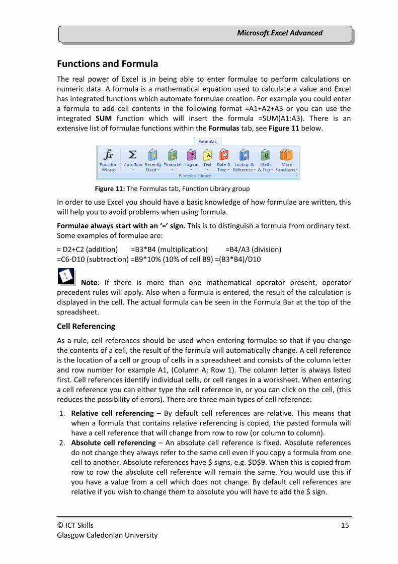
Functions and Formula The real power of Excel is in being able to enter formulae to perform calculations on numeric data. A formula is a mathematical equation used to calculate a value and Excel has integrated functions which automate formulae creation. For example you could enter a formula to add cell contents in the following format =A1+A2+A3 or you can use the integrated SUM function which will insert the formula =SUM(A1:A3). There is an extensive list of formulae functions within the Formulas tab, see Figure 11 below.

Figure 11: The Formulas tab, Function Library group

In order to use Excel you should have a basic knowledge of how formulae are written, this will help you to avoid problems when using formula.

Formulae always start with an ‘=’ sign. This is to distinguish a formula from ordinary text. Some examples of formulae are:

= D2+C2 (addition) =B3*B4 (multiplication) =B4/A3 (division) =C6‐D10 (subtraction) =B9*10% (10% of cell B9) =(B3*B4)/D10

Note: If there is more than one mathematical operator present, operator precedent rules will apply. Also when a formula is entered, the result of the calculation is displayed in the cell. The actual formula can be seen in the Formula Bar at the top of the spreadsheet.

Cell Referencing

As a rule, cell references should be used when entering formulae so that if you change the contents of a cell, the result of the formula will automatically change. A cell reference is the location of a cell or group of cells in a spreadsheet and consists of the column letter and row number for example A1, (Column A; Row 1). The column letter is always listed first. Cell references identify individual cells, or cell ranges in a worksheet. When entering a cell reference you can either type the cell reference in, or you can click on the cell, (this reduces the possibility of errors). There are three main types of cell reference:

1. Relative cell referencing – By default cell references are relative. This means that when a formula that contains relative referencing is copied, the pasted formula will have a cell reference that will change from row to row (or column to column).

2. Absolute cell referencing – An absolute cell reference is fixed. Absolute references do not change they always refer to the same cell even if you copy a formula from one cell to another. Absolute references have $ signs, e.g. $D$9. When this is copied from row to row the absolute cell reference will remain the same. You would use this if you have a value from a cell which does not change. By default cell references are relative if you wish to change them to absolute you will have to add the $ sign.



3. Mixed cell referencing ‐ A mixed cell reference has either an absolute column and a relative row, or an absolute row and a relative column. $A1 is an example of a mixed reference where the column will not change but the row number will.

Sum Function/Formula

The SUM formula as mentioned earlier can be used to add the content of cells in either columns or rows. To use the SUM formula, move the cursor to the cell which will contain the result of the addition then type in the formula, for example =A1+B1+C1. This formula would add together the contents of cell A1, B1 and C1 and return the answer in the designated cell. To use the SUM function within Excel, choose the cell which will contain

the results of the addition and click on the AutoSum command from the Formulas tab, Function Library group, see Figure 11 below. Excel will suggest which cells have to be added together by showing the selection in a broken line and entering the formula in the cell. If the suggestion is correct press ENTER . If not, type in the correct range of cells separated by a colon, e.g. A5:A10 or B10:F10, or highlight the range using the mouse. The SUM function will be displayed as =SUM(A5:A10).

Average Function/Formula

When working with data you may also wish to find out the average number in a data set. For example it may be useful to find out the average mark scored by students who have undertaken the ICT Skills module. To do this you can either type the formula in the cell you wish to contain the answer, or you can use the AVERAGE function which is found in

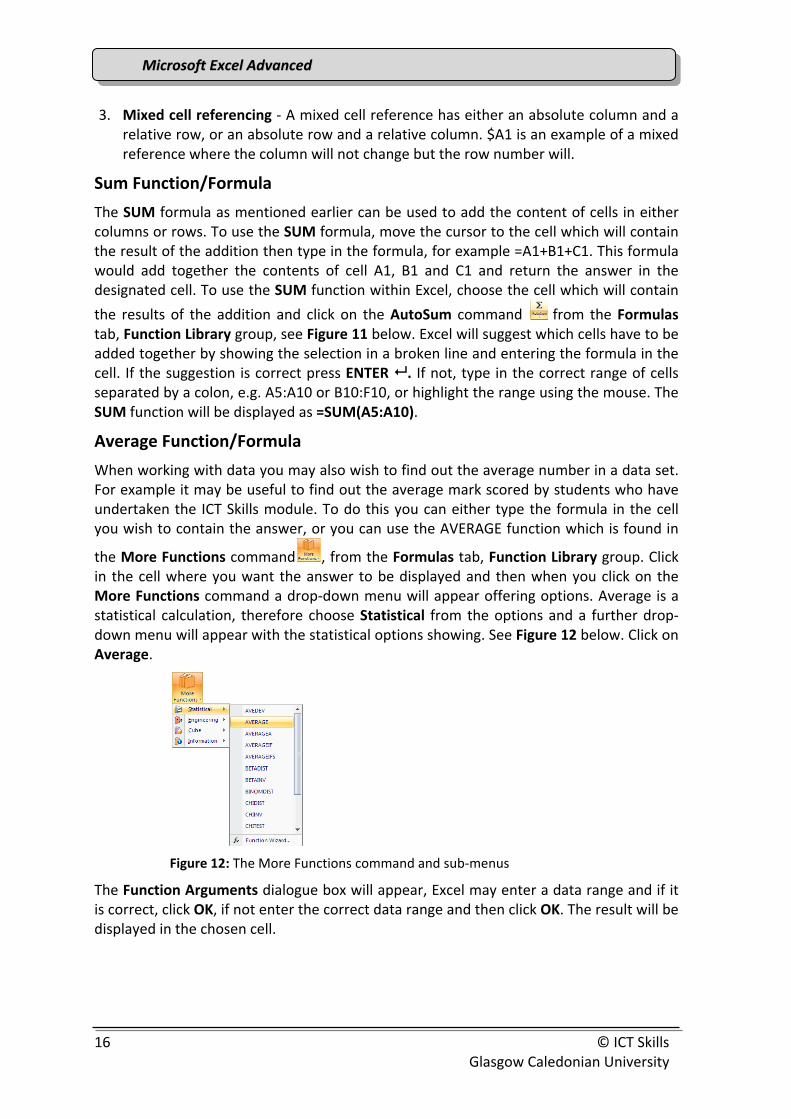
the More Functions command , from the Formulas tab, Function Library group. Click in the cell where you want the answer to be displayed and then when you click on the More Functions command a drop‐down menu will appear offering options. Average is a statistical calculation, therefore choose Statistical from the options and a further drop‐down menu will appear with the statistical options showing. See Figure 12 below. Click on Average.

Figure 12: The More Functions command and sub‐menus

The Function Arguments dialogue box will appear, Excel may enter a data range and if it is correct, click OK, if not enter the correct data range and then click OK. The result will be displayed in the chosen cell.



Figure 13: The Function Arguments dialogue box

Conditional (Logical) Function/Formula

These are formula which use the IF; AND; OR; NOT operators to test whether a condition is true or false.

• IF: returns one value if the condition is true and another if it is false

• AND: If all of the conditions are true then TRUE will be returned. If one or more of the conditions are false then FALSE will be returned.

• OR: If any of the conditions are true then TRUE will be returned.

• NOT: If the condition is true NOT returns FALSE; If the condition is false NOT returns TRUE.

Once the true or false condition is determined a corresponding value will be returned. For example if you wanted to check if a student had scored enough to pass a module you could use a conditional formula to compare the value in the cell with the pass mark. If the mark is equal to or above the pass mark then you could display the value you wish to return for that (PASS), if it is false you could display another value (FAIL).

You can structure a conditional formula in a number of ways by using the operators listed above. One of the most common conditional formulae is the IF formula.

IF

The IF formula is used within Excel to test whether the contents of a cell meet certain criteria specified by you, and then return a value on that basis. This formula has three main parts:

1. LOGICAL_ TEST: This is what the formula is using to decide which value to return

2. VALUE_ IF_ TRUE: This value will be returned if the condition is met (is TRUE)

3. VALUE_ IF_ FALSE: This value will be returned if the condition is not met (is FALSE)

An IF formula therefore would consist of the following:

=IF(logical_test, value_if_true, value_if_false)

Task 10

Use the Average function to calculate the Average mark of students on the ICT Skills module in the emptied cell.

The data range will be entered or displayed in this field.



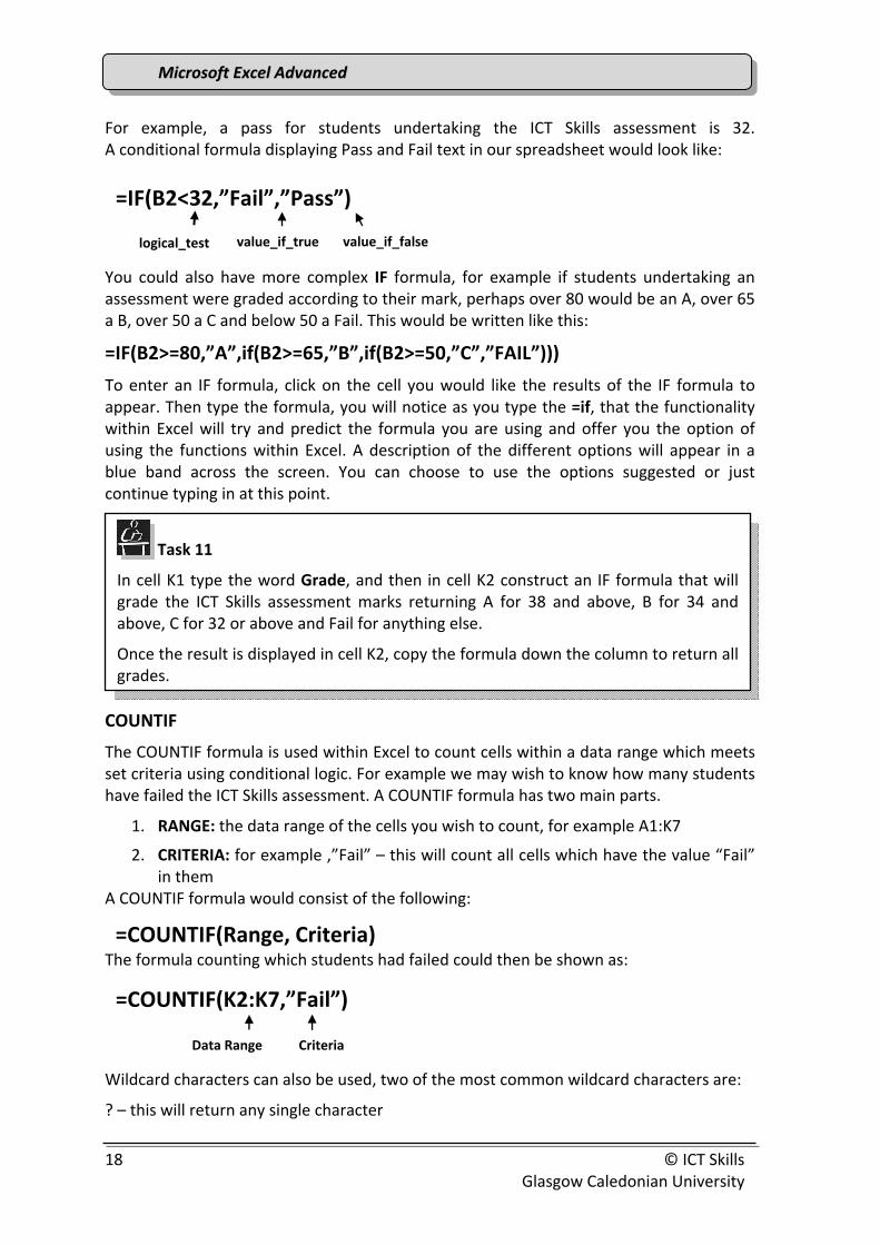
For example, a pass for students undertaking the ICT Skills assessment is 32. A conditional formula displaying Pass and Fail text in our spreadsheet would look like:

You could also have more complex IF formula, for example if students undertaking an assessment were graded according to their mark, perhaps over 80 would be an A, over 65 a B, over 50 a C and below 50 a Fail. This would be written like this:

=IF(B2>=80,”A”,if(B2>=65,”B”,if(B2>=50,”C”,”FAIL”)))

To enter an IF formula, click on the cell you would like the results of the IF formula to appear. Then type the formula, you will notice as you type the =if, that the functionality within Excel will try and predict the formula you are using and offer you the option of using the functions within Excel. A description of the different options will appear in a blue band across the screen. You can choose to use the options suggested or just continue typing in at this point.

COUNTIF

The COUNTIF formula is used within Excel to count cells within a data range which meets set criteria using conditional logic. For example we may wish to know how many students have failed the ICT Skills assessment. A COUNTIF formula has two main parts.

1. RANGE: the data range of the cells you wish to count, for example A1:K7

2. CRITERIA: for example ,”Fail” – this will count all cells which have the value “Fail” in them

A COUNTIF formula would consist of the following:

=COUNTIF(Range, Criteria) The formula counting which students had failed could then be shown as:

Wildcard characters can also be used, two of the most common wildcard characters are:

? – this will return any single character

=COUNTIF(K2:K7,”Fail”)

Data Range Criteria

Task 11

In cell K1 type the word Grade, and then in cell K2 construct an IF formula that will grade the ICT Skills assessment marks returning A for 38 and above, B for 34 and above, C for 32 or above and Fail for anything else.

Once the result is displayed in cell K2, copy the formula down the column to return all grades.

=IF(B2<32,”Fail”,”Pass”)

logical_test value_if_true value_if_false



* ‐ this will return a sequence of characters.

To use COUNTIF, place the cursor in the cell in which you wish the results to show and type in the formula. Alternately click on the Formulas tab, Function Library group and More Functions command. A drop‐down menu with options will appear. COUNTIF is a statistical function so click on this option. A further drop‐down menu appears, choose the COUNTIF function, see Figure 14 below.

Figure 14: More Functions Command, with drop‐down menus

The Function Arguments dialogue box will appear as shown in Figure 15 below.

Figure 15: The Function Arguments dialogue box.

Enter the data range in the Range field, this will be in the format A1:B7 and the criteria of the cells you wish to count in the Criteria field. This can be a number, a range of numbers or letter(s) or wildcard characters. Then click on OK. The count should now appear in the cell selected by you.

Task 12

In an empty cell on the spreadsheet create a COUNTIF formula which will count the number of students from the BAAC course code who have undertaken the ICT Skills Assessment.



LOOK UP Function

You can use Excel to “look up” and then return a value in a list or in a table. After the value has been looked up it can be used for calculations. This can be useful to ensure the accuracy and validity of information and eliminate data entry errors. There are different ways of looking up values in a list and displaying the results. The two most popular functions are, the VLOOKUP where the V stands for vertical and HLOOKUP where the H stands for horizontal. Both work in much the same way therefore just the VLOOKUP function will be described.

Vertical LOOKUP (VLOOKUP)

The VLOOKUP formula, searches the values in the vertical columns of a list or table for a specified value, column by column from the left side. This data is then copied and can be returned elsewhere in the worksheet/book. There are four basic arguments in this function:

=VLOOKUP(lookup_value,table_array,col_index_num,[range_lookup]) 1. LOOK UP VALUE: Identifies the value to be looked up, this could be a number, a

string of text or an actual cell reference. In the lookup_value section enter the value that you wish to look up. You can do this by either clicking on the cell which contains the value, or typing the value in.

2. THE TABLE ARRAY: The cell range containing the data. This is normally in the format A1:D10, it is recommended that when you use a cell range that you make the cell references absolute by inserting the $ sign in front of them (see the description on p 15).

3. THE COL_INDEX_NUM: An index number to identify the column (or the row in case of HLOOKUP) from which the value will come. This is the column within the table which contains the data you are looking for.

4. THE RANGE LOOKUP: This is a non compulsory option. A range lookup specifies whether there is an exact match or an approximate match for the search. If you wish an EXACT match you must put FALSE in this section. If you wish an APPROXIMATE match to be found (the largest value that is less than the lookup_value) then TRUE should be entered.

To look up a value you must firstly click in the destination cell. That is the cell in which you wish the result of your lookup to be displayed. Then from the Formula tab choose the Lookup and Reference command. When you click on this a drop‐down list displaying the various functions will show. Choose the VLOOKUP option, see Figure 16 below.

Figure 16: the Lookup and Reference command and drop‐down menu



The Function Arguments dialogue box will appear as in Figure 17 below. Enter the function arguments as required. Then click on OK.

Figure 17: Function Arguments dialogue box

For example, from the table we have currently created you could use a VLOOKUP function and look up the Matric no of a student from the table and return their course code. To do this you would:

1. Open your workbook if it is not already open.

2. Type the label(s) for your lookup. In this case it would be:

a. Enter a Matric no (cell A9)

b. Course Code (cell A10)

3. Use the VLOOKUP function in the destination cell (B10) and enter all of the arguments. Press Enter or click OK

The formula you would enter in cell B10 would be:

=VLOOKUP(B9,A1:K7,4,FALSE) Or the arguments you would enter in the Function Arguments dialogue box would be:

• Lookup_ value: B9 (Excel will go to cell B9 for the value entered there)

• Table_array: A1:K7, (the cell range of the table)

• Col_index_num: 4 (the column number which contains the data you would like returned)

• Range_lookup: False (an exact match for your lookup value must be found. For this particular example we would require an exact match, for many others an approximate would be required)

Note: You will receive #N/A answer in your cell until you enter a matriculation number in cell B9.



VLOOKUP Errors

If you find once you have entered your formula that you have an error indication in your returns (#N/A) check the validity of the data you have entered. Common reasons for error messages are:

Exact and approximate values. If you specify that you wish the function to return an exact value and that exact value does not exist this may then lead to an error.

Missing Data: If you use a value that does not exist then you will be given an error message. When the formula searched the table for the value it was missing, an error message was then generated.

Unsorted Data: When you use a VLOOKUP function the value will be looked up from a sorted list, if the list is not sorted this may cause an error message to be generated.

Custom/worksheet function used that is not available: If you have created the lookup formula using a customised function it may not be available on all versions of the application. If you then use another computer which does not have the updated functionality you may not be able to access it.

SUBTOTALS

The subtotal function can be used to perform calculations on data that has been sorted and filtered. When data is sorted and filtered (see p.10 to p.12) it appears to limit the data available, however any calculations carried out on this data will include hidden rows. The subtotal function will insert totals into groups of data but will only calculate the visible cells, hidden cells will be ignored. You can subtotal a sorted/filtered list so that only the visible cells are added or you can use the other subtotal functions to perform calculations such as those listed in the table below.

Function Use AVERAGE Calculates the arithmetic mean of a group. COUNT Counts the number of entries in a group. MAX Returns the maximum value in a group. MIN Returns the minimum value in a group. PRODUCT Multiplies values in a group. STDDEV Estimates standard deviation of the samples of a group. STDDEVP Calculates standard deviation of a group. SUM Calculated the sum of the values in a group. VAR Estimates the variance of the samples of a group. VARP Calculates the variance of a group.

Task 13

Type the labels, Enter a Matric No in cell A9, and Phone No in A10.

Using a VLOOKUP formula or function, search the workbook by matriculation number to return the phone number for students.



To add subtotals to a sorted/filtered list click on a cell within the list. Then from the Data tab, Outline group click on the Subtotal command, see Figure 18 below.

Figure 18: The Outline group within the Data tab

The subtotal dialogue box will appear, see Figure 19 below.

Figure 19: The Subtotal dialogue box.

The dialogue box gives options for you to choose in which column you would like the subtotals to be grouped by. You will be asked to choose a subtotal function. You may wish the subtotals to be added or averaged or to show the maximum/minimum value. A full list of functions and there use is shown in the table above. Select a function from the drop‐down list. Finally you should choose which columns this operation should be applied to by choosing from the options displayed in the list shown. Check the box which applies. You also have the option to choose to replace current subtotals, insert page breaks between subtotals and to include a summary below the data. If you do not tick the Summary below data option check box, you will not see a grand total in your spreadsheet.

Task 14

Create subtotals for students who have passed the ICT Skills module.

Display the average mark by Course Code.

Save and close the spreadsheet.

Subtotal command



Charts and Graphs A chart is a visual depiction of information. Excel contains an easy‐to‐use function to create graphs and charts which allows you to display information contained within a spreadsheet as a chart or graph. Displaying raw Excel data in a well constructed chart can make the data more understandable, meaningful and can be useful for summarising data and spotting trends.

Chart Types and Uses

There are many different types of charts and graphs including line graphs, pie charts, column charts and scatter charts, and it is vitally important that the correct chart type is chosen.

Note: Choosing the wrong chart type can lead to the data being misinterpreted.

Column/Bar Charts

These are probably the most common chart types and are used for comparing data. A column chart displays vertical columns, where each column represents one of the values/categories being compared. A sub type of the column chart is the stacked column chart and the main difference is that a stacked column chart shows the amount each category contributes to the total, as in the diagram. The bar chart is the same but instead of vertical columns it shows horizontal bars.

Line Charts Line charts are most commonly used to display trends in data, and show continuous data over a set time period. This chart displays each value/category as a point, the points are connected by lines.

Pie Charts Pie charts are often used to show values/categories as a percentage of the total. A pie chart is displayed as a circle which is broken into segments, the size of each segment is determined by it’s percentage of the total. You can determine the most important “value” within a data set using a pie chart.

XY Scatter Charts XY scatter charts can be used to plot workbook data showing relationships/comparisons between the data values. An XY scatter chart can be used to display comparisons or relationships between two data values.



Creating a Chart

A chart can be created in the worksheet you are working on or in a separate sheet of the workbook. Constructing a chart or graph involves the following steps:

1. Choose the data range (data to be charted). To select the data range, use the mouse to highlight all of the data you want to appear on the chart. If you want to select two non‐adjacent rows or columns, hold down the CTRL key when selecting the data.

2. Choose the type of chart/graph required. To do this, click the Insert tab, and on the chart type command from the Chart group, see Figure 20.

Figure 20: The Charts group of the Insert tab

3. When a chart type command is chosen a drop‐down menu for that chart type will be shown displaying all of the different types within that command, see Figure 21 below. Rest the mouse on any option for a description of the chart type. Click on the chart type you wish to use.

Figure 21: Column chart types

4. The chart will be displayed in the worksheet currently displayed (see Figure 22). If you would like the chart to show in another existing workbook or a separate sheet

click on the Move Chart command in the Chart Tools ‐ Design tab.



Figure 22: Chart contained within Spreadsheet

5. Add labels to the chart by changing the layout of the chart (more detailed explanation is given later on p.30). To do this click on the chart and then go to the Chart Tools ‐ Design tab. Click on the more button in the Chart Layouts group to see all chart layouts. Click on the Layout you want (make sure it has Chart and Axis Titles). Excel will now change the layout of the chart and will put the default titles.

6. Click on the default Chart Title and type an appropriate title for you chart in the Formula Bar. Do the same for the Axis Titles.

Moving and Resizing a Chart

When your chart is created and inserted into the current worksheet sometimes it covers the data. If this happens you can move the chart to an empty area on the worksheet. To

Task 15

Open Excel and enter the following:

Course Code Student Nos Pass Fail

BAAC 445 385 60

BSOO 358 300 58

BARM 650 548 102

BSIS 259 200 59

MSIS 300 217 83

Create a column chart showing the Pass and Fail rate for each programme. Add appropriate titles and labels. Save as Charts.xlsx

Chart Tools tabs

Chart

Axes: Y and X

Legend

Data charted, non adjacent in this example.

Move Chart command



do this, move the cursor to the chart, when the cursor changes to a four headed arrow, click on any white area within the chart and hold and drag the chart to the new location.

Sometimes when a chart is inserted into a worksheet not all of the data can be seen. If this happens the chart can be resized. The sizing handles of the chart can be found at the borders of the chart and are shown with dots. To resize the chart, move the mouse to the edges. When you do this the cursor will change to a double headed arrow. Click, hold and drag the chart frame resizing handles to the size required.

The elements of the chart can also be resized. Click any of the elements i.e. the title box, the legend box or the chart itself and drag to the required size.

Sometimes it is easier to operate with the chart if it is in a separate sheet in your workbook. You can move your chart to a new sheet by clicking on the Move Chart command in the Chart Tools – Design tab, Location group. Use the same command to move it back from a separate sheet to the sheet where the data is taken from. When you click on the Move Chart command a dialogue box will appear (see Figure 23 below). Choose the appropriate option and click OK to move the chart to the location specified.

Figure 23: Move Chart dialogue box

Inserting/Modifying a Chart Title

Once you have created your chart you may wish to insert or change the title. To do this, ensure the chart is selected and then from Chart Tools – Layout tab, Labels group choose

Task 18

Use the Autosum ∑ function to total all Passes and all Fails in the spreadsheet.

Create a pie chart from showing all passes and all fails. Move the chart to a new worksheet in your workbook.

Task 17

Resize the chart to ensure all of the data is showing. Increase the font size of the title and resize the box if needed to ensure the title is showing.

Task 16

Move the column chart to below the table.



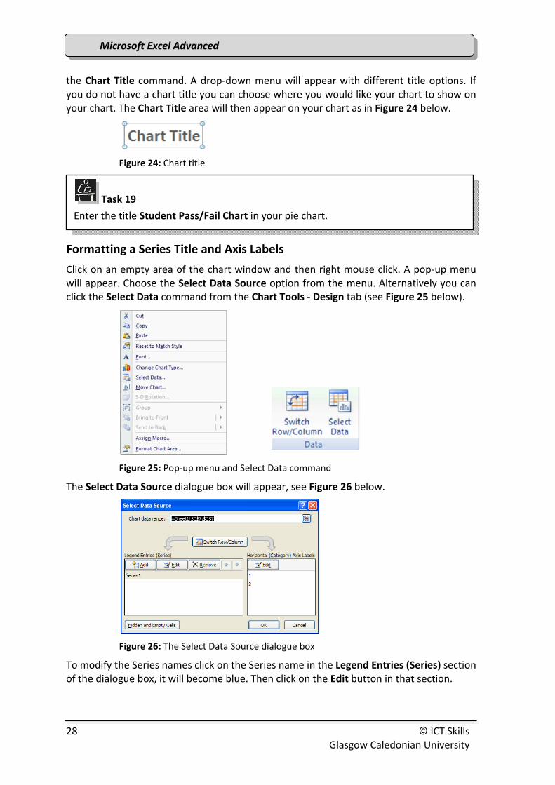
the Chart Title command. A drop‐down menu will appear with different title options. If you do not have a chart title you can choose where you would like your chart to show on your chart. The Chart Title area will then appear on your chart as in Figure 24 below.

Figure 24: Chart title

Formatting a Series Title and Axis Labels

Click on an empty area of the chart window and then right mouse click. A pop‐up menu will appear. Choose the Select Data Source option from the menu. Alternatively you can click the Select Data command from the Chart Tools ‐ Design tab (see Figure 25 below).

Figure 25: Pop‐up menu and Select Data command

The Select Data Source dialogue box will appear, see Figure 26 below.

Figure 26: The Select Data Source dialogue box

To modify the Series names click on the Series name in the Legend Entries (Series) section of the dialogue box, it will become blue. Then click on the Edit button in that section.

Task 19

Enter the title Student Pass/Fail Chart in your pie chart.



The Edit Series dialogue box will then appear (see Figure 27). In the Series name: field type the name you wish for your Series and click OK and the chart will then appear with the Series name changed.

Figure 27: Edit Series dialogue box

To modify the chart axis labels click on the Edit button in the Horizontal (Category)Axis Labels section of the Select Data Source dialogue box. The Axis Labels dialogue box will open (see Figure 28). You can now select from your worksheet the labels (all of them) that you want displayed. Click OK when you have finished and then OK to close the Select Data Source dialogue box. The chart will now show the data with the labels that you have selected.

Figure 28: Axis Labels dialogue box

Modifying Charts

The functionality within Excel allows you to customise the appearance of the chart, and to ensure the display is appealing and appropriate to the audience it is aimed at.

If you have created a chart and then feel that you have chosen the wrong chart type you can change it. To do this, ensure your chart is selected by clicking on it. The Chart Tools contextual tabs will appear, i.e. Design, Layout and Format. Click on the Chart Tools ‐ Design tab, Type group and Change Chart Type command (see Figure 29 below).

Figure 29: Chart Type commands

Task 20

Using the Select Data Source and modify the Axis Labels of your pie chart as described above to show Pass and Fail.



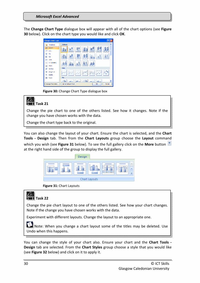
The Change Chart Type dialogue box will appear with all of the chart options (see Figure 30 below). Click on the chart type you would like and click OK.

Figure 30: Change Chart Type dialogue box

You can also change the layout of your chart. Ensure the chart is selected, and the Chart Tools ‐ Design tab. Then from the Chart Layouts group choose the Layout command

which you wish (see Figure 31 below). To see the full gallery click on the More button at the right hand side of the group to display the full gallery.

Figure 31: Chart Layouts

You can change the style of your chart also. Ensure your chart and the Chart Tools ‐ Design tab are selected. From the Chart Styles group choose a style that you would like (see Figure 32 below) and click on it to apply it.

Task 22

Change the pie chart layout to one of the others listed. See how your chart changes. Note if the change you have chosen works with the data.

Experiment with different layouts. Change the layout to an appropriate one.

Note: When you change a chart layout some of the titles may be deleted. Use Undo when this happens.

Task 21

Change the pie chart to one of the others listed. See how it changes. Note if the change you have chosen works with the data.

Change the chart type back to the original.



Figure 32: Chart Styles group

To see the full range of chart styles available click on the More button at the right hand side of the gallery. Choose the style you wish to use and click on it. Your chart style will now be changed.

Formatting Charts

The chart can also be formatted by using the commands available within the Chart Tools ‐ Format tab option (see Figure 33 below).

Figure 33: Chart Tools ‐Format tab

The different shapes within the chart can be formatted by clicking on it, i.e. a column in a column chart, segment of a pie chart, a legend etc and choosing one of the formatting options. If you wished to change the chart axes to give them more emphasis you could use the WordArt options within the WordArt Styles group. To do this click on the chart axes. A box with sizing handles will appear around the chosen axis. Click one of the

WordArt options. To see all of the WordArt commands use the More button at the end of the WordArt Styles group. Click on the command you wish to use.

The layout of the chart elements may also be changed. If you did not require a legend, but would rather include a data table in your chart you can do this. Firstly ensure the chart is selected, from the Chart Tools ‐ Layout tab, Labels group choose the Legend command (see Figure 34 below). A drop‐down menu will appear with all of the legend options available, choose None. The legend from your chart will disappear. Then choose

Task 24

Use the WordArt option to change the axes of your pie chart.

Experiment with different options and choose a suitable one.

Task 23

Change the pie chart style chosen to one of the others listed. See how your chart changes.

Experiment with different styles. Change the style to an appropriate one.



the Data Table option, a drop‐down list with all options will appear. Choose the Show Data Table option. A data table will appear at the bottom of the chart.

Figure 34: The Chart Tools ‐ Layout tab

PivotTables PivotTables are used in Excel to summarise data and present the information in report format. PivotTable reports allow large volumes of data to be split into small concise reports. When creating a PivotTable report it is important to remember that each column heading in your workbook will become a field name in the report. Column headings must therefore be appropriate. Also when creating a PivotTable report it is best to ensure your data has no blank columns or rows.

To create a PivotTable report, click in a cell in your spreadsheet, or select only the data you wish for your report. Then from the Insert tab, Tables group click on the top half of the PivotTable command (or if you click at the bottom half choose PivotTable from the menu that will appear), see Figure 35 below.

Figure 35: Table group and PivotTable command

The Create PivotTable dialogue box will open, the data source chosen earlier will be showing in the Select a table or range, Table/Range field. Choose where the PivotTable report should be displayed within the workbook with the default option being in a New Worksheet (see Figure 36 below).

Figure 36: Create PivotTable dialogue box

Click OK. Your PivotTable report layout will be created and look like Figure 37 below.

Select a table or range

Where will the PivotTable report show

Task 25

Remove the legend from your column chart, and add a data table.



Figure 37: PivotTable Report worksheet

The PivotTable Report layout will be displayed in the left hand side of the worksheet and the Pivot Table Field List pane will have opened at the right hand side. Select the fields you wish to add to your report by checking the box next to the field name in the Pivot Table Field List pane. You should notice the data appearing in your PivotTable. Excel will automatically assign the value(s) to the four smaller areas below the PivotTable Field List pane.

Excel by default assigns values to the correct areas below the PivotTable Field List pane. If, however, you wish them to be in another area you can change the area by dragging and dropping the value to the area you wish. Alternately click on the value that you wish to move and a menu will appear for you to choose the option you wish.

Note: The data in the PivotTable will change as you move the values around.

Which fields you add to your PivotTable will depend on what you would like to report on. For example, if you would like to know the number of students from each course you would add the Course Code and Student Nos fields to the PivotTable.

You can also add fields to your report to expand on it, you could perhaps create a PivotTable report which shows the average mark of the students on each programme and the average overall mark. To do this add the Programme Code and Mark fields to your PivotTable Report. Excel will assign them to the areas and add them to the PivotTable. By default the Value is SUM (∑), however you can choose another value for the field. To do this click on the field name, a pop up menu will appear (see Figure 38 below).

Task 26

Create a PivotTable Report from the Charts workbook showing pass rates for each course.

Save and close the Charts workbook.

Report Filter: The data value you wish to filter your report by.

PivotTable Tools tabs PivotTable Field List: This will contain the fields from the data source. You must check the boxes to include them in your PivotTable

Values



Figure 38: Values pop up menu

Choose Value Field Settings… from this menu, the Value Field Settings dialogue box will appear (see Figure 39 below).

Figure 39: Value Field Settings dialogue box

Excel will insert a custom name for the value, if you do not wish this name change it to the one you wish. Then choose which calculation type you would like from the menu at the bottom and click OK. The calculation will be performed on your chosen field.

If the data you have is large you may not be able to see all of the entries. To enable you to see the entries more clearly you can Pivot the information. To pivot the information you move the information from the Rows area at the bottom of the Pivot Field List pane to the Columns. This changes the layout of the information.

Task 28

Pivot the table to show Courses in the columns.

Save and close the ICT Student Data spreadsheet.

Task 27

Create a PivotTable report in the ICT Student Data spreadsheet which shows the average marks for each programme.

Documents

Excel Advanced 07 - GCU · 2019-01-30 · Vertical LOOKUP (VLOOKUP) ... Excel is a spreadsheet application used for storing number and text data and for performing numerical calculations