Excel 2010 –Tips & Tricks - pc knowledge llcpcknowledgellc.com/wp-content/uploads/2012/04/Tips_and_Tricks_10... · pc knowledge, llc Excel 2010 – Tips & Tricks Page 2 When you

Speeding Productivity

pc knowledge, llc

829 Purser Drive / Raleigh, NC 27603

(919)999‐6503

Presented by: Phil Faucette, PE

Excel2010– Tips&Tricks

pc knowledge, llc Excel 2010 – Tips & Tricks Page 1

Excel Tables

Excel Table is an exciting new feature in MS Excel™ Versions 2007/2010!

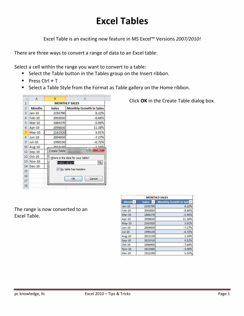
There are three ways to convert a range of data to an Excel table:

Select a cell within the range you want to convert to a table: Select the Table button in the Tables group on the Insert ribbon.

Press Ctrl + T . Select a Table Style from the Format as Table gallery on the Home ribbon.

Click OK in the Create Table dialog box.

The range is now converted to an Excel Table.


When you type in a cell adjacent to a table, Excel automatically adds it to the table and formats the top row or left column cell to match. When you add a formula to the new column and hit Enter Excel automatically fills the formula to entire Column.

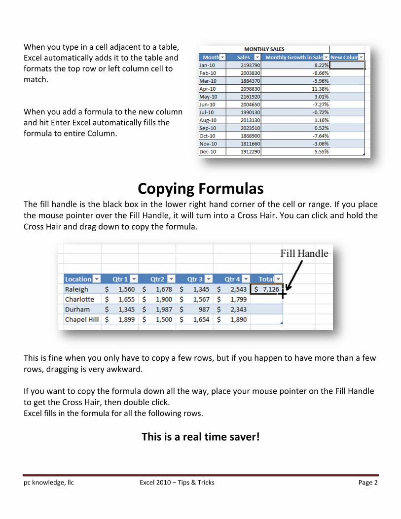
Copying Formulas The fill handle is the black box in the lower right hand corner of the cell or range. If you place the mouse pointer over the Fill Handle, it will tum into a Cross Hair. You can click and hold the Cross Hair and drag down to copy the formula.

This is fine when you only have to copy a few rows, but if you happen to have more than a few rows, dragging is very awkward.

If you want to copy the formula down all the way, place your mouse pointer on the Fill Handle to get the Cross Hair, then double click. Excel fills in the formula for all the following rows.

This is a real time saver!


Answers in a Hurry!

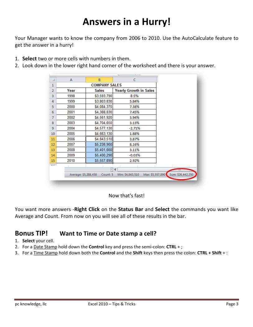
Your Manager wants to know the company from 2006 to 2010. Use the AutoCalculate feature to get the answer in a hurry!

1. Select two or more cells with numbers in them. 2. Look down in the lower right hand corner of the worksheet and there is your answer.

Now that's fast!

You want more answers ‐Right Click on the Status Bar and Select the commands you want like Average and Count. From now on you will see all of these results in the bar.

Bonus TIP! Want to Time or Date stamp a cell? 1. Select your cell. 2. For a Date Stamp hold down the Control key and press the semi‐colon: CTRL + ; 3. For a Time Stamp hold down both the Control and the Shift keys then press the colon: CTRL + Shift + :


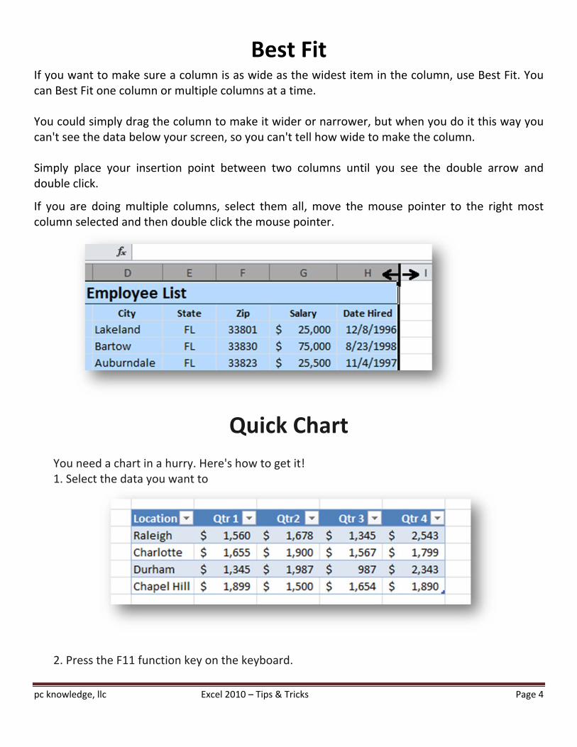
Best Fit If you want to make sure a column is as wide as the widest item in the column, use Best Fit. You can Best Fit one column or multiple columns at a time.

You could simply drag the column to make it wider or narrower, but when you do it this way you can't see the data below your screen, so you can't tell how wide to make the column.

Simply place your insertion point between two columns until you see the double arrow and double click.

If you are doing multiple columns, select them all, move the mouse pointer to the right most column selected and then double click the mouse pointer.

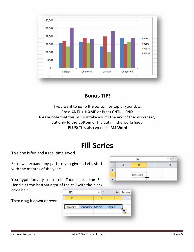
Quick Chart You need a chart in a hurry. Here's how to get it! 1. Select the data you want to

2. Press the F11 function key on the keyboard.


Bonus TIP!

If you want to go to the bottom or top of your data,

Press CNTL + HOME or Press CNTL + END Please note that this will not take you to the end of the worksheet,

but only to the bottom of the data in the worksheet. PLUS: This also works in MS Word

Fill Series

This one is fun and a real time saver!

Excel will expand any pattern you give it. Let's start with the months of the year:

You type January in a cell. Then select the Fill Handle at the bottom right of the cell with the black cross hair.

Then drag it down or over.


If you want to get 1,2,3 etc. you have to give it a pattern of 1 and 2. If you want 2,4,6,8, etc. you have to give it a pattern of 2 and 4.

Caution: A common mistake is having just a single cell pattern. Computers are dumb, you have to tell it Exactly what you want!

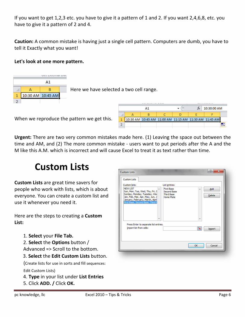
Let's look at one more pattern.

Here we have selected a two cell range.

When we reproduce the pattern we get this.

Urgent: There are two very common mistakes made here. (1) Leaving the space out between the time and AM, and (2) The more common mistake ‐ users want to put periods after the A and the M like this A.M. which is incorrect and will cause Excel to treat it as text rather than time.

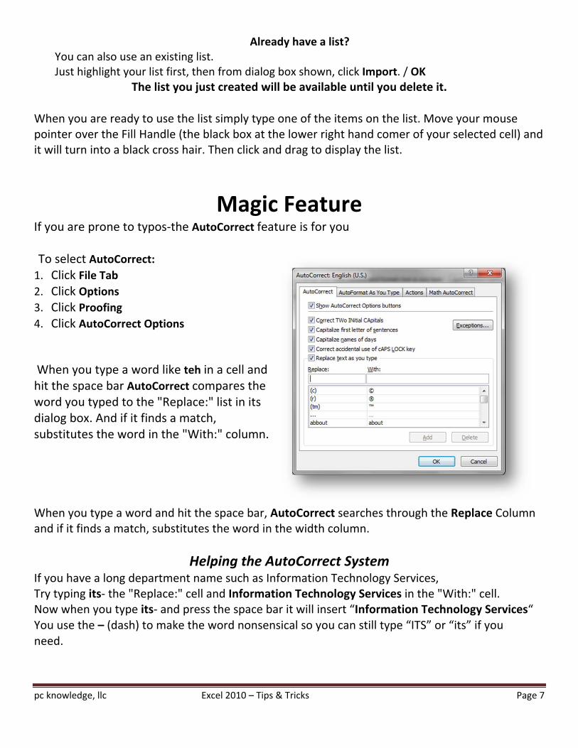
Custom Lists

Custom Lists are great time savers for people who work with lists, which is about everyone. You can create a custom list and use it whenever you need it.

Here are the steps to creating a Custom List:

1. Select your File Tab. 2. Select the Options button / Advanced => Scroll to the bottom.

3. Select the Edit Custom Lists button.

(Create lists for use in sorts and fill sequences:

Edit Custom Lists)

4. Type in your list under List Entries 5. Click ADD. / Click OK.


Already have a list? You can also use an existing list. Just highlight your list first, then from dialog box shown, click Import. / OK

The list you just created will be available until you delete it.

When you are ready to use the list simply type one of the items on the list. Move your mouse pointer over the Fill Handle (the black box at the lower right hand comer of your selected cell) and it will turn into a black cross hair. Then click and drag to display the list.

Magic Feature If you are prone to typos‐the AutoCorrect feature is for you

To select AutoCorrect: 1. Click File Tab 2. Click Options 3. Click Proofing 4. Click AutoCorrect Options

When you type a word like teh in a cell and hit the space bar AutoCorrect compares the word you typed to the "Replace:" list in its dialog box. And if it finds a match, substitutes the word in the "With:" column. When you type a word and hit the space bar, AutoCorrect searches through the Replace Column and if it finds a match, substitutes the word in the width column.

Helping the AutoCorrect System If you have a long department name such as Information Technology Services, Try typing its‐ the "Replace:" cell and Information Technology Services in the "With:" cell. Now when you type its‐ and press the space bar it will insert “Information Technology Services“ You use the – (dash) to make the word nonsensical so you can still type “ITS” or “its” if you need.


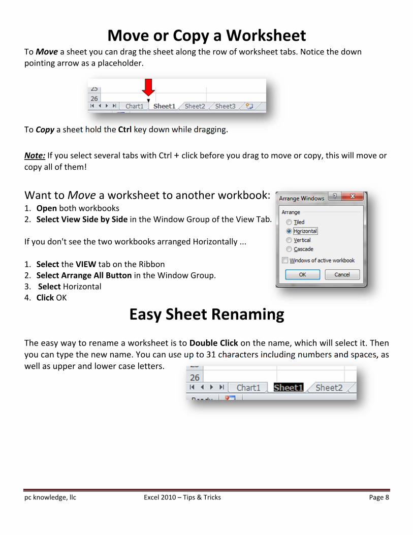
Move or Copy a Worksheet To Move a sheet you can drag the sheet along the row of worksheet tabs. Notice the down pointing arrow as a placeholder.

To Copy a sheet hold the Ctrl key down while dragging.

Note: If you select several tabs with Ctrl + click before you drag to move or copy, this will move or

copy all of them!

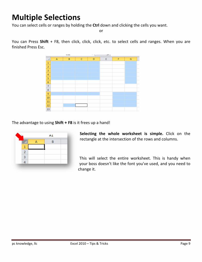
Want to Move a worksheet to another workbook: 1. Open both workbooks 2. Select View Side by Side in the Window Group of the View Tab. If you don't see the two workbooks arranged Horizontally ...

1. Select the VIEW tab on the Ribbon 2. Select Arrange All Button in the Window Group. 3. Select Horizontal 4. Click OK

Easy Sheet Renaming

The easy way to rename a worksheet is to Double Click on the name, which will select it. Then you can type the new name. You can use up to 31 characters including numbers and spaces, as well as upper and lower case letters.


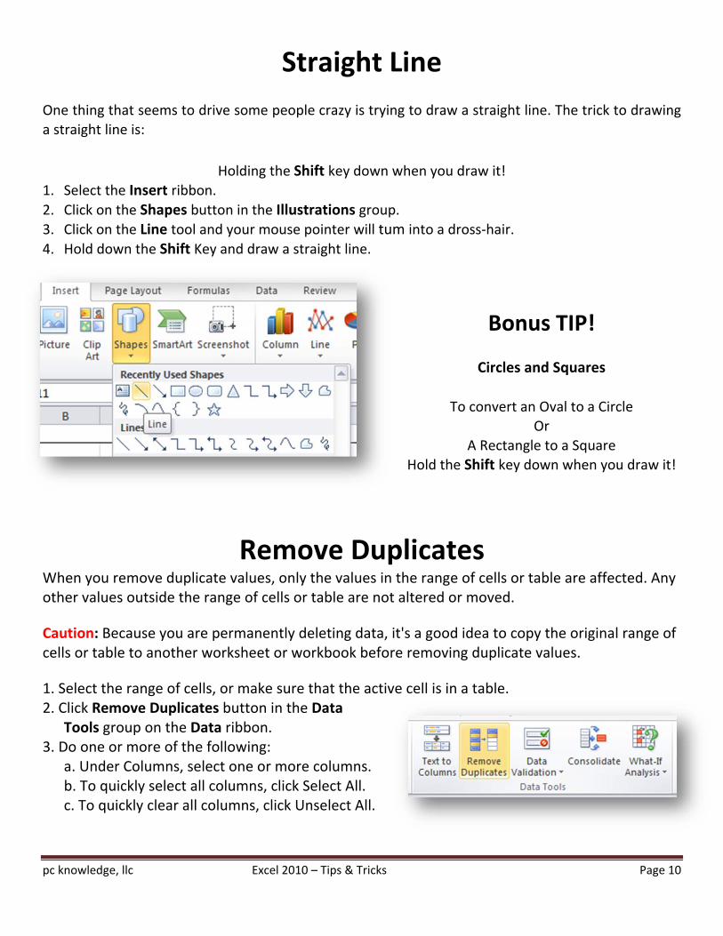
Multiple Selections You can select cells or ranges by holding the Ctrl down and clicking the cells you want.

or

You can Press Shift + F8, then click, click, click, etc. to select cells and ranges. When you are finished Press Esc.

The advantage to using Shift + F8 is it frees up a hand!

Selecting the whole worksheet is simple. Click on the rectangle at the intersection of the rows and columns.

This will select the entire worksheet. This is handy when your boss doesn't like the font you've used, and you need to change it.


Straight Line

One thing that seems to drive some people crazy is trying to draw a straight line. The trick to drawing

a straight line is:

Holding the Shift key down when you draw it! 1. Select the Insert ribbon. 2. Click on the Shapes button in the Illustrations group. 3. Click on the Line tool and your mouse pointer will tum into a dross‐hair. 4. Hold down the Shift Key and draw a straight line.

Bonus TIP!

Circles and Squares

To convert an Oval to a Circle

Or

A Rectangle to a Square

Hold the Shift key down when you draw it!

Remove Duplicates

When you remove duplicate values, only the values in the range of cells or table are affected. Any other values outside the range of cells or table are not altered or moved. Caution: Because you are permanently deleting data, it's a good idea to copy the original range of cells or table to another worksheet or workbook before removing duplicate values. 1. Select the range of cells, or make sure that the active cell is in a table. 2. Click Remove Duplicates button in the Data

Tools group on the Data ribbon. 3. Do one or more of the following:

a. Under Columns, select one or more columns. b. To quickly select all columns, click Select All. c. To quickly clear all columns, click Unselect All.


Note: If the range of cells or table contains many columns and you want to only select a few columns, you may find it easier to click Unselect All, and then under Columns, select those columns. 4. Click OK. Note: A message is displayed indicating how many duplicate values were removed and how many unique values remain, or if no duplicate values were removed.

5. Click OK.

** Please Note **

You cannot remove duplicate values from data that is outlined or that has subtotals. To remove duplicates, you must remove both the outline and the subtotals.

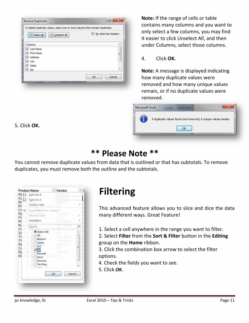
Filtering

This advanced feature allows you to slice and dice the data many different ways. Great Feature!

1. Select a cell anywhere in the range you want to filter. 2. Select Filter from the Sort & Filter button in the Editing group on the Home ribbon. 3. Click the combination box arrow to select the filter options. 4. Check the fields you want to see. 5. Click OK.


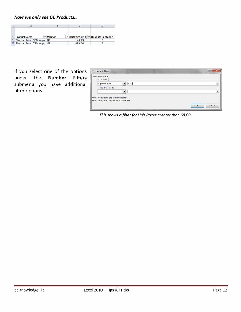
Now we only see GE Products…

If you select one of the options under the Number Filters submenu you have additional filter options.

This shows a filter for Unit Prices greater than $8.00.

Documents

Excel 2010 –Tips & Tricks - pc knowledge llcpcknowledgellc.com/wp-content/uploads/2012/04/Tips_and_Tricks_10... · pc knowledge, llc Excel 2010 – Tips & Tricks Page 2 When you