Excel 2007 Manual. Describe the components of an Excel worksheet. 3. Move within the worksheet. 4. ... Along with the new features of Microsoft Excel 2007 come several

Introduction to

Excel 2007

Technology Training Services

i

Introduction to Excel 2007

Written by Kathleen A. Moser, PhD

Technology Training Services

Revised August 2009

Maricopa County Community College District © August, 2009

The Maricopa County Community College District is an EEO/AA institution.

This training manual may be duplicated or put on the Internet for instructional purposes. Please give credit to the Maricopa Community Colleges and to the

author(s). This training manual is not to be sold for profit.

Technology Training Services Maricopa Community Colleges

2411 West 14th Street Tempe, Arizona 85281-6942 (480) 731-8287 http://www.maricopa.edu/training

ii

Technology Training Services Vision & Mission

Technology Training Services improves employee job performance at all levels by exceeding expectations in the areas of technology training, instructional design, and customer support. Technology Training Services provides leadership and support to the Maricopa Community College District as the District implements new technologies that address challenging administrative needs and educational standards. We design, develop, and deliver the highest quality in-service technology training, materials, and support to all of the employees of the Maricopa Community Colleges. To fulfill this mission we: • Provide responsive and accessible technology training on a

variety of administrative systems and desktop applications.

• Design and develop comprehensive training and reference materials.

• Provide technology training support in a variety of ways including telephone help lines, one-on-one assistance, online help, troubleshooting, consultation, and referral services.

• Support the colleges' technology training efforts by delivering on-site technology training, delivering Train-the-Trainer sessions, and providing training materials.

• Provide leadership and support to the teams implementing new technologies and administrative systems within the organization.

• Cultivate positive partnerships with our colleges to meet and exceed their training needs and expectations.

• Collaborate with organizational teams to develop strategies to meet future technology training needs.

• Chair and host the Regional Training Committee (RTC) to collaboratively develop training strategies, maintain technology training consistency, and overcome the challenging technology training needs throughout the District.

• Expand and update our knowledge and skills in the areas of technology, training, and instructional design.

Vision

Mission

iii

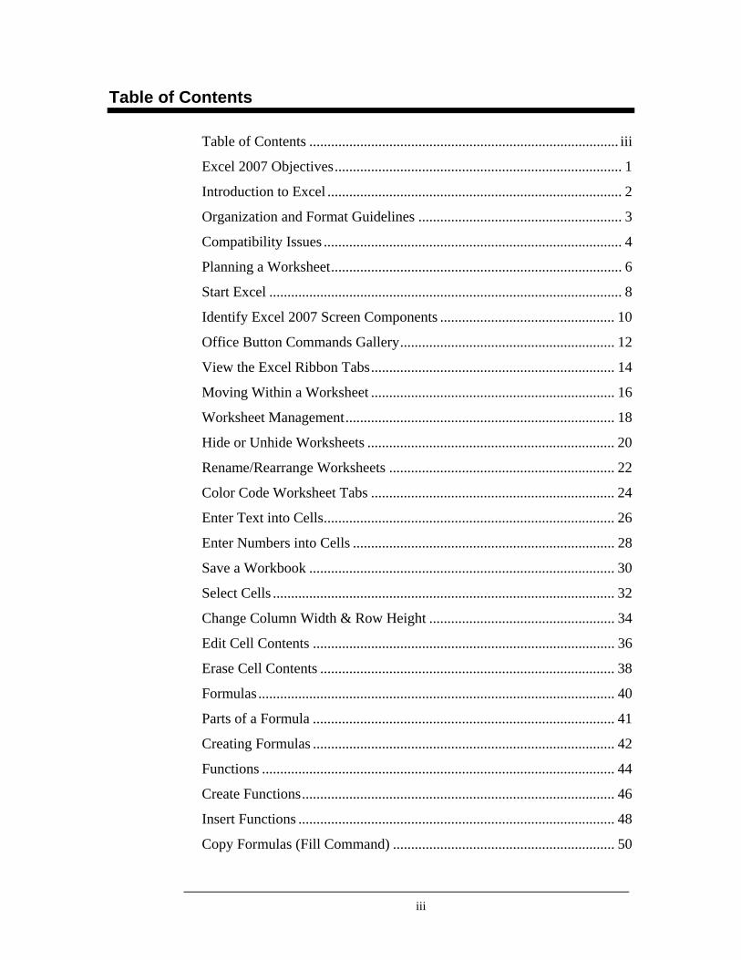
Table of Contents

Table of Contents ..................................................................................... iii

Excel 2007 Objectives ............................................................................... 1

Introduction to Excel ................................................................................. 2

Organization and Format Guidelines ........................................................ 3

Compatibility Issues .................................................................................. 4

Planning a Worksheet ................................................................................ 6

Start Excel ................................................................................................. 8

Identify Excel 2007 Screen Components ................................................ 10

Office Button Commands Gallery ........................................................... 12

View the Excel Ribbon Tabs ................................................................... 14

Moving Within a Worksheet ................................................................... 16

Worksheet Management .......................................................................... 18

Hide or Unhide Worksheets .................................................................... 20

Rename/Rearrange Worksheets .............................................................. 22

Color Code Worksheet Tabs ................................................................... 24

Enter Text into Cells ................................................................................ 26

Enter Numbers into Cells ........................................................................ 28

Save a Workbook .................................................................................... 30

Select Cells .............................................................................................. 32

Change Column Width & Row Height ................................................... 34

Edit Cell Contents ................................................................................... 36

Erase Cell Contents ................................................................................. 38

Formulas .................................................................................................. 40

Parts of a Formula ................................................................................... 41

Creating Formulas ................................................................................... 42

Functions ................................................................................................. 44

Create Functions ...................................................................................... 46

Insert Functions ....................................................................................... 48

Copy Formulas (Fill Command) ............................................................. 50

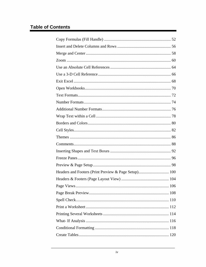
iv

Table of Contents

Copy Formulas (Fill Handle) .................................................................. 52

Insert and Delete Columns and Rows ..................................................... 56

Merge and Center .................................................................................... 58

Zoom ....................................................................................................... 60

Use an Absolute Cell References ............................................................ 64

Use a 3-D Cell Reference ........................................................................ 66

Exit Excel ................................................................................................ 68

Open Workbooks ..................................................................................... 70

Text Formats ............................................................................................ 72

Number Formats ...................................................................................... 74

Additional Number Formats .................................................................... 76

Wrap Text within a Cell .......................................................................... 78

Borders and Colors .................................................................................. 80

Cell Styles ................................................................................................ 82

Themes .................................................................................................... 86

Comments ................................................................................................ 88

Inserting Shapes and Text Boxes ............................................................ 92

Freeze Panes ............................................................................................ 96

Preview & Page Setup ............................................................................. 98

Headers and Footers (Print Preview & Page Setup) .............................. 100

Headers & Footers (Page Layout View) ............................................... 104

Page Views ............................................................................................ 106

Page Break Preview ............................................................................... 108

Spell Check ............................................................................................ 110

Print a Worksheet .................................................................................. 112

Printing Several Worksheets ................................................................. 114

What- If Analysis .................................................................................. 116

Conditional Formatting ......................................................................... 118

Create Tables ......................................................................................... 120

v

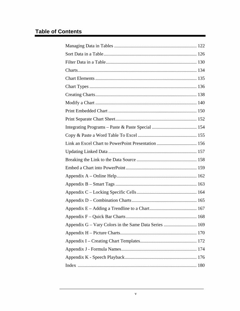
Table of Contents

Managing Data in Tables ...................................................................... 122

Sort Data in a Table ............................................................................... 126

Filter Data in a Table ............................................................................. 130

Charts ..................................................................................................... 134

Chart Elements ...................................................................................... 135

Chart Types ........................................................................................... 136

Creating Charts ...................................................................................... 138

Modify a Chart ...................................................................................... 140

Print Embedded Chart ........................................................................... 150

Print Separate Chart Sheet ..................................................................... 152

Integrating Programs – Paste & Paste Special ...................................... 154

Copy & Paste a Word Table To Excel .................................................. 155

Link an Excel Chart to PowerPoint Presentation .................................. 156

Updating Linked Data ........................................................................... 157

Breaking the Link to the Data Source ................................................... 158

Embed a Chart into PowerPoint ............................................................ 159

Appendix A – Online Help .................................................................... 162

Appendix B – Smart Tags ..................................................................... 163

Appendix C – Locking Specific Cells ................................................... 164

Appendix D – Combination Charts ....................................................... 165

Appendix E – Adding a Trendline to a Chart ........................................ 167

Appendix F – Quick Bar Charts ............................................................ 168

Appendix G – Vary Colors in the Same Data Series ............................ 169

Appendix H – Picture Charts ................................................................. 170

Appendix I – Creating Chart Templates ................................................ 172

Appendix J - Formula Names ................................................................ 174

Appendix K - Speech Playback ............................................................. 176

Index ..................................................................................................... 180

1

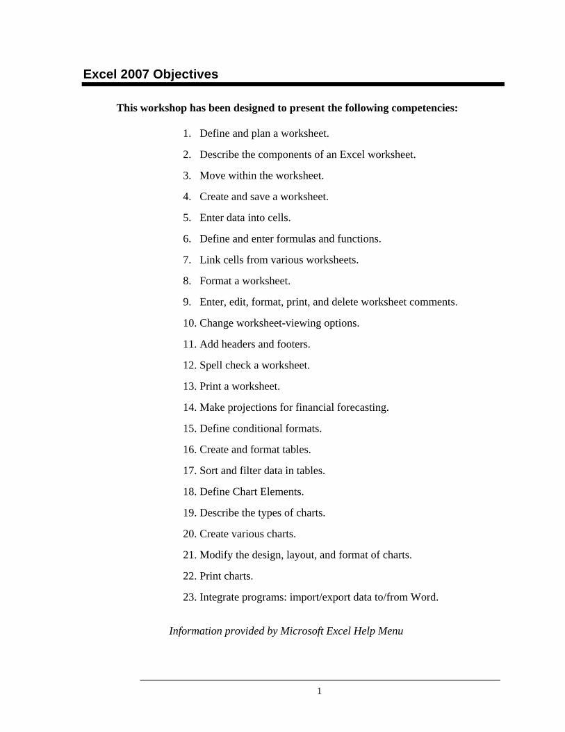
Excel 2007 Objectives

This workshop has been designed to present the following competencies:

1. Define and plan a worksheet.

2. Describe the components of an Excel worksheet.

3. Move within the worksheet.

4. Create and save a worksheet.

5. Enter data into cells.

6. Define and enter formulas and functions.

7. Link cells from various worksheets.

8. Format a worksheet.

9. Enter, edit, format, print, and delete worksheet comments.

10. Change worksheet-viewing options.

11. Add headers and footers.

12. Spell check a worksheet.

13. Print a worksheet.

14. Make projections for financial forecasting.

15. Define conditional formats.

16. Create and format tables.

17. Sort and filter data in tables.

18. Define Chart Elements.

19. Describe the types of charts.

20. Create various charts.

21. Modify the design, layout, and format of charts.

22. Print charts.

23. Integrate programs: import/export data to/from Word.

Information provided by Microsoft Excel Help Menu

2

Introduction to Excel

Microsoft Excel 2007 is a powerful tool you can use to create, organize, analyze and present data to make more informed decisions. The flat data structure of spreadsheets (data not related to other data as in Access 2007) is easy to create and easy to maintain so long as you don’t have too much information.

If data analysis is your primary goal, Excel is the program for you. The power of Excel 2007 is with numbers. You can run sophisticated what-if models and cost-benefit analyses. Conveying information visually through professional-looking charts with visual effects helps to identify key data trends.

Data is organized into rows and columns in a document called a worksheet. Several worksheets can be combined and saved in a file called a workbook. This concept is similar to a book that contains several pages. For example, a company’s annual budget is contained in a workbook that contains several worksheets; one worksheet for each quarter.

Entries in a worksheet are placed in a cell, which is the intersection of a column and a row. A cell is identified by the column letter and row number, such as A1. Worksheets can be created to track, analyze, and chart any data set up in this format. For example, expenses, sales, grades, assets, liabilities, statistics, and gas usage are the types of information that can be stored and analyzed in a worksheet.

The power of Excel 2007 is in performing what-if analysis. Once a worksheet has been created, you can test what happens to quarterly cash flow if you alter your budget to include a new employee or give your employees a 3 percent raise. You simply add or edit a value and observe as Excel’s recalculation feature automatically updates all values dependent on the numbers you are forecasting.

Microsoft Excel 2007 has several features that make it easy to manage and analyze data. To take full advantage of these features, it is important that you plan, organize, and format your data according to a few easy to follow guidelines.

Numbers!

Just like a book

What-if Analysis

3

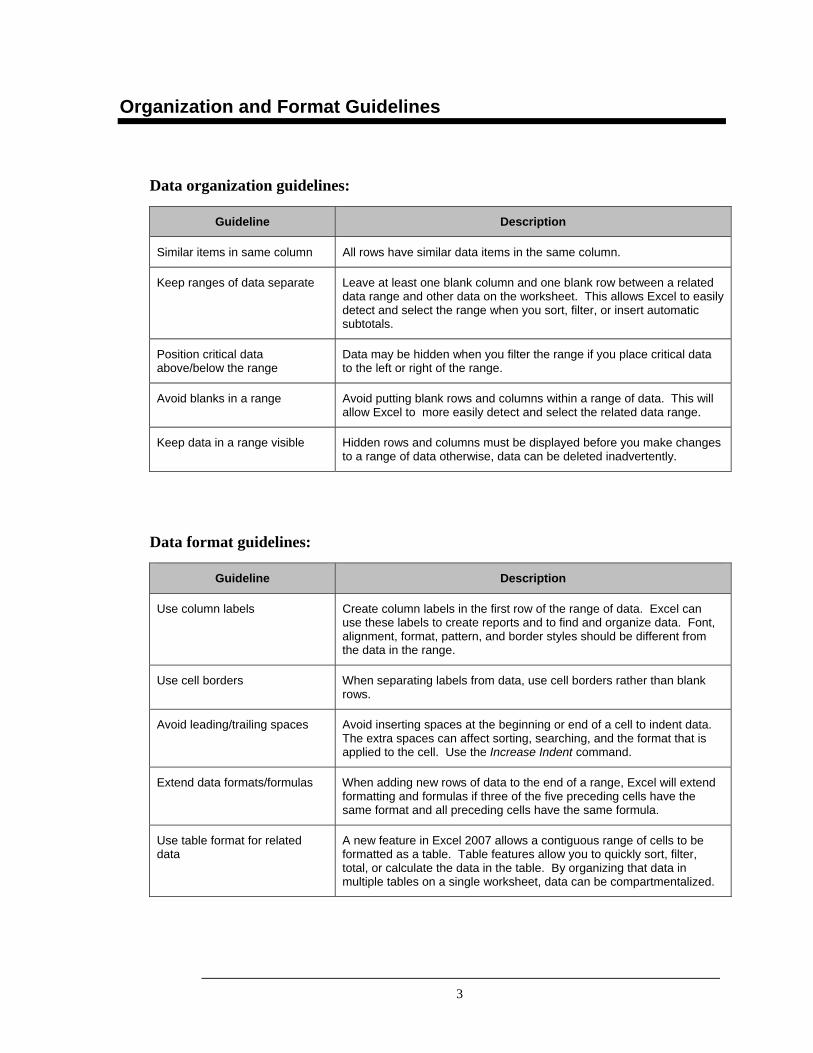
Organization and Format Guidelines

Data organization guidelines:

Guideline Description

Similar items in same column All rows have similar data items in the same column.

Keep ranges of data separate Leave at least one blank column and one blank row between a related data range and other data on the worksheet. This allows Excel to easily detect and select the range when you sort, filter, or insert automatic subtotals.

Position critical data above/below the range

Data may be hidden when you filter the range if you place critical data to the left or right of the range.

Avoid blanks in a range Avoid putting blank rows and columns within a range of data. This will allow Excel to more easily detect and select the related data range.

Keep data in a range visible Hidden rows and columns must be displayed before you make changes to a range of data otherwise, data can be deleted inadvertently.

Data format guidelines:

Guideline Description

Use column labels Create column labels in the first row of the range of data. Excel can use these labels to create reports and to find and organize data. Font, alignment, format, pattern, and border styles should be different from the data in the range.

Use cell borders When separating labels from data, use cell borders rather than blank rows.

Avoid leading/trailing spaces Avoid inserting spaces at the beginning or end of a cell to indent data. The extra spaces can affect sorting, searching, and the format that is applied to the cell. Use the Increase Indent command.

Extend data formats/formulas When adding new rows of data to the end of a range, Excel will extend formatting and formulas if three of the five preceding cells have the same format and all preceding cells have the same formula.

Use table format for related data

A new feature in Excel 2007 allows a contiguous range of cells to be formatted as a table. Table features allow you to quickly sort, filter, total, or calculate the data in the table. By organizing that data in multiple tables on a single worksheet, data can be compartmentalized.

4

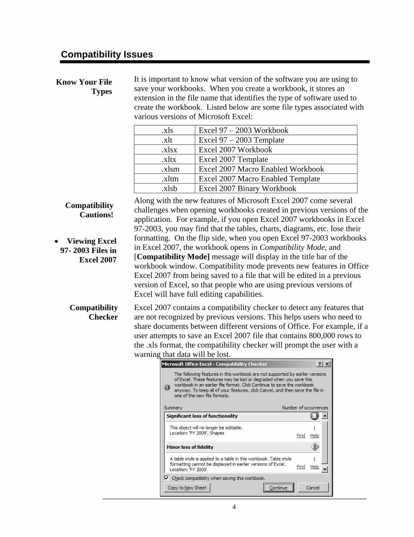
Compatibility Issues

It is important to know what version of the software you are using to save your workbooks. When you create a workbook, it stores an extension in the file name that identifies the type of software used to create the workbook. Listed below are some file types associated with various versions of Microsoft Excel:

.xls Excel 97 – 2003 Workbook .xlt Excel 97 – 2003 Template .xlsx Excel 2007 Workbook .xltx Excel 2007 Template .xlsm Excel 2007 Macro Enabled Workbook .xltm Excel 2007 Macro Enabled Template .xlsb Excel 2007 Binary Workbook

Along with the new features of Microsoft Excel 2007 come several challenges when opening workbooks created in previous versions of the application. For example, if you open Excel 2007 workbooks in Excel 97-2003, you may find that the tables, charts, diagrams, etc. lose their formatting. On the flip side, when you open Excel 97-2003 workbooks in Excel 2007, the workbook opens in Compatibility Mode, and [Compatibility Mode] message will display in the title bar of the workbook window. Compatibility mode prevents new features in Office Excel 2007 from being saved to a file that will be edited in a previous version of Excel, so that people who are using previous versions of Excel will have full editing capabilities.

Excel 2007 contains a compatibility checker to detect any features that are not recognized by previous versions. This helps users who need to share documents between different versions of Office. For example, if a user attempts to save an Excel 2007 file that contains 800,000 rows to the .xls format, the compatibility checker will prompt the user with a warning that data will be lost.

Know Your File Types

Compatibility Cautions!

• Viewing Excel 97- 2003 Files in

Excel 2007

Compatibility Checker

5

Compatibility Issues

Consider the following when sharing different Excel files types. • Save the workbook down to Excel 97 – 2003. This will allow

all individuals to be able to open the workbook and make the appropriate edits.

• Download the Office Compatibility Pack on to computers with Excel 97 – 2003 version. This will allow users to open an Excel 2007 workbook for viewing purposes.

The Office 2007 Compatibility Pack is a plug-in that allows Excel 97-2003 users to open a workbook created in Excel 2007. Some formatting may be lost when opening a 2007 workbook in a lower format. For additional information visit the website listed below. http://www.microsoft.com/downloads/details.aspx?familyid=941B3470-3AE9-4AEE-8F43-C6BB74CD1466&displaylang=en

Converting your workbook allows you to access the new and enhanced features in Office Excel 2007.

It is strongly recommended that you perform the following functions to maintain the integrity of your workbooks when upgrading to Excel 2007.

• Convert your existing workbooks to Excel 2007.

o Make a copy of the workbook created in the previous version of Excel without opening the workbook.

o Avoid using the double-click method to open a Excel 97-2003 workbook. Instead, open Excel 2007, open the Excel 97-2003 workbook, and then save the workbook as an Excel 2007 workbook.

o Create a new blank workbook, copy and paste the information from the old version into the new version.

• Save all new workbooks in Excel 2007.

File Sharing Considerations

• Viewing Excel 2007 Files in

Excel 97- 2003

File Conversion Considerations

6

Planning a Worksheet

Planning and designing your worksheet will save time when creating, organizing, and formatting your data. Determining what you want to accomplish, who will use your data and how they will view it will guide you in establishing the formats, formulas, functions, and visual effects needed in your design.

For example, if you are using the worksheet to calculate course grades, you need to develop the formulas that the worksheet will use to compute grades. Is a simple averaging of the course test scores all that is needed, or will a weighted average of test scores, extra credit work, team projects and presentations be measured? Will any data need to be grouped to show correlations? Will the worksheet transform a numerical grade to a letter grade? Will you need charts to illustrate comparisons between diverse data groups?

Sample questions to help you plan a worksheet include:

1. What is the purpose of the worksheet?

2. Are multiple worksheets needed?

3. Who will use the worksheet(s)?

4. What data is necessary?

5. How will the information be organized and formatted?

6. What calculations are needed?

7. What information is needed in order to perform those calculations?

8. Will charts be used to illustrate trends or comparisons?

9. Does the data need to be sorted or filtered to be viewed by different groups of people?

10. Are the processes recurring (weekly, monthly, quarterly, or annually)?

Planning serves a vital role in helping to avoid mistakes or recognize hidden opportunities. With a plan in place, you are more able to clarify and focus on the project's development, understand more clearly what you want to achieve, and how and when to accomplish it.

Establish goals Begin with the

End in mind

Planning Tips

7

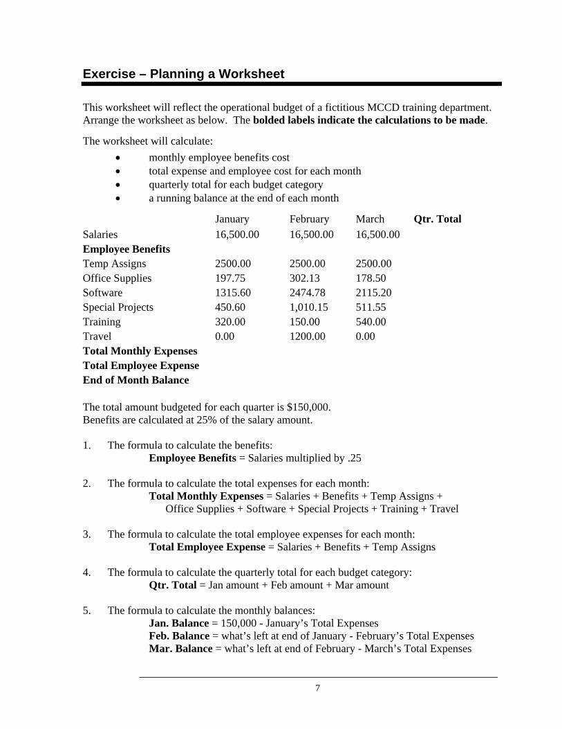
Exercise – Planning a Worksheet

This worksheet will reflect the operational budget of a fictitious MCCD training department. Arrange the worksheet as below. The bolded labels indicate the calculations to be made.

The worksheet will calculate: • monthly employee benefits cost • total expense and employee cost for each month • quarterly total for each budget category • a running balance at the end of each month

January February March Qtr. Total Salaries 16,500.00 16,500.00 16,500.00 Employee Benefits Temp Assigns 2500.00 2500.00 2500.00 Office Supplies 197.75 302.13 178.50 Software 1315.60 2474.78 2115.20 Special Projects 450.60 1,010.15 511.55 Training 320.00 150.00 540.00 Travel 0.00 1200.00 0.00 Total Monthly Expenses Total Employee Expense End of Month Balance The total amount budgeted for each quarter is $150,000. Benefits are calculated at 25% of the salary amount. 1. The formula to calculate the benefits: Employee Benefits = Salaries multiplied by .25 2. The formula to calculate the total expenses for each month: Total Monthly Expenses = Salaries + Benefits + Temp Assigns +

Office Supplies + Software + Special Projects + Training + Travel

3. The formula to calculate the total employee expenses for each month: Total Employee Expense = Salaries + Benefits + Temp Assigns 4. The formula to calculate the quarterly total for each budget category: Qtr. Total = Jan amount + Feb amount + Mar amount 5. The formula to calculate the monthly balances: Jan. Balance = 150,000 - January’s Total Expenses Feb. Balance = what’s left at end of January - February’s Total Expenses Mar. Balance = what’s left at end of February - March’s Total Expenses

8

Start Excel

When Excel is opened, it creates an empty workbook and gives the file a generic name of Book1. A workbook is like a notebook containing many sheets of paper called worksheets. Each worksheet can contain data and charts. Initially the workbook is defaulted to contain 3 worksheets. Additional sheets can be inserted as needed.

The worksheet may be thought of as a grid, which is divided into columns and rows. Alphabetic letters displayed horizontally across the top of the window designate the columns. Vertical numbers displayed down the left side of the window designate the rows. Data is entered into a cell, which is the intersection of a column with a row.

Each worksheet in Excel contains 16,384 columns and 1,048,576 rows.

At the Windows Desktop, click the start button on the Taskbar. Choose Microsoft Office Excel 2007 from the start menu. If Microsoft Excel 2007 is not pinned to the start menu the program may be launched through the All Programs option on the start menu.

At the Windows Desktop, click the start button on the Taskbar. Choose the All Programs option from the start menu. Click Microsoft Office and then click Microsoft Office Excel 2007.

You will be creating a quarterly budget report for the MCCD training department, Technology Development Center (TDC) on the previous page.

1. Click the Start button on the Taskbar to display the Start menu.

2. Point to Microsoft Excel 2007 on the start menu.

OR

3. Click the Start button on the Taskbar to display the Start menu.

4. Point to All Programs to display the program group submenu.

5. Click Microsoft Office.

6. Click Microsoft Office Excel 2007.

Workbooks and Worksheets

Starting Excel

Step to Start Excel

9

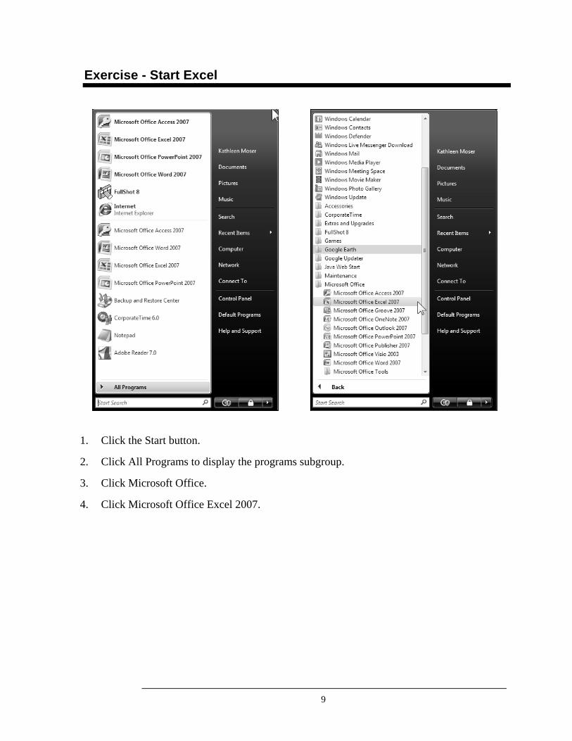
Exercise - Start Excel

1. Click the Start button.

2. Click All Programs to display the programs subgroup.

3. Click Microsoft Office.

4. Click Microsoft Office Excel 2007.

10

Identify Excel 2007 Screen Components

Microsoft Excel 2007 has a new look which is identified as a Fluent User Interface. It includes the Office Button, the Quick Access Toolbar, and the Ribbon. The features of the interface and other screen components are described below. Displays the name you give the workbook after you save it. The Office button provides a central location for commands that represent all of the things you can do with an entire workbook, such as open, close, save, print, publish, etc. It has replaced the File Menu, found in earlier versions. The Quick Access Toolbar allows you to keep a customized set of tools handy; and it always displays, regardless of what tab is selected on the Ribbon, or even when the Ribbon is minimized. The largest new component of the Fluent User interface is the Ribbon, which provides a graphical representation of tools and replaces the traditional menus and toolbars in earlier versions. As you position your mouse over each button in the Ribbon and hold your mouse still, a Screen Tip (formerly known as a Tool Tip) appears to tell you the name of the button. Marks the point at which text will be inserted when you begin typing. You will see a blinking cursor at this spot. The blue bar displayed at the bottom of the Excel spreadsheet. The status bar provides a convenient method of summing, averaging and counting a range of cells, and provides status message like ready, calculate, found etc. It now includes shortcut buttons for the worksheet views and a handy Zoom Slider to adjust the on-screen size of your worksheet. The Sheet Tabs at the bottom of the screen are used to move from worksheet to worksheet within the workbook. Clicking Sheet Tab will activate the desired worksheet. Sheet tabs can be deleted, renamed, rearranged, colored and grouped as needed. Horizontal (bottom of window) and Vertical (right side of window) Scroll Bars may be used to scroll through the worksheet. The Excel Help window contains links to categories of help topics. You can click a category link, or search for a word or phrase.

Fluent User Interface

Title Bar

Office Button

Quick Access Toolbar

Ribbon

Screen Tips

Insertion Point

Status Bar

Sheet Tabs

Scroll Bars

Excel Help

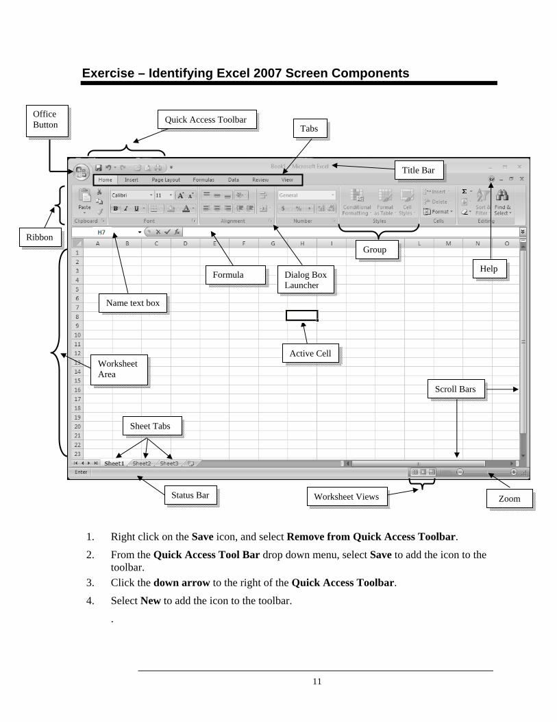
11

Exercise – Identifying Excel 2007 Screen Components

1. Right click on the Save icon, and select Remove from Quick Access Toolbar.

2. From the Quick Access Tool Bar drop down menu, select Save to add the icon to the toolbar.

3. Click the down arrow to the right of the Quick Access Toolbar.

4. Select New to add the icon to the toolbar.

.

Tabs

Status Bar Worksheet Views Zoom

Formula Help

Quick Access ToolbarOffice Button

Name text box

Active Cell

Sheet Tabs

Title Bar

Group

Worksheet Area

Ribbon

Dialog Box Launcher

Scroll Bars

12

Office Button Commands Gallery

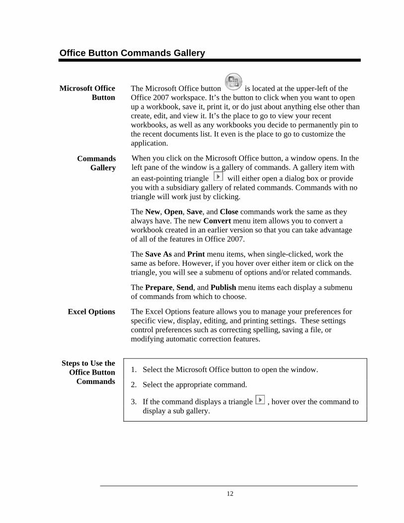
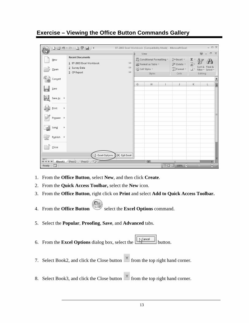
The Microsoft Office button is located at the upper-left of the Office 2007 workspace. It’s the button to click when you want to open up a workbook, save it, print it, or do just about anything else other than create, edit, and view it. It’s the place to go to view your recent workbooks, as well as any workbooks you decide to permanently pin to the recent documents list. It even is the place to go to customize the application.

When you click on the Microsoft Office button, a window opens. In the left pane of the window is a gallery of commands. A gallery item with an east-pointing triangle will either open a dialog box or provide you with a subsidiary gallery of related commands. Commands with no triangle will work just by clicking.

The New, Open, Save, and Close commands work the same as they always have. The new Convert menu item allows you to convert a workbook created in an earlier version so that you can take advantage of all of the features in Office 2007.

The Save As and Print menu items, when single-clicked, work the same as before. However, if you hover over either item or click on the triangle, you will see a submenu of options and/or related commands.

The Prepare, Send, and Publish menu items each display a submenu of commands from which to choose.

The Excel Options feature allows you to manage your preferences for specific view, display, editing, and printing settings. These settings control preferences such as correcting spelling, saving a file, or modifying automatic correction features.

1. Select the Microsoft Office button to open the window.

2. Select the appropriate command.

3. If the command displays a triangle , hover over the command to display a sub gallery.

Microsoft Office Button

Commands Gallery

Excel Options

Steps to Use the Office Button

Commands

13

Exercise – Viewing the Office Button Commands Gallery

1. From the Office Button, select New, and then click Create.

2. From the Quick Access Toolbar, select the New icon.

3. From the Office Button, right click on Print and select Add to Quick Access Toolbar.

4. From the Office Button select the Excel Options command.

5. Select the Popular, Proofing, Save, and Advanced tabs.

6. From the Excel Options dialog box, select the button.

7. Select Book2, and click the Close button from the top right hand corner.

8. Select Book3, and click the Close button from the top right hand corner.

14

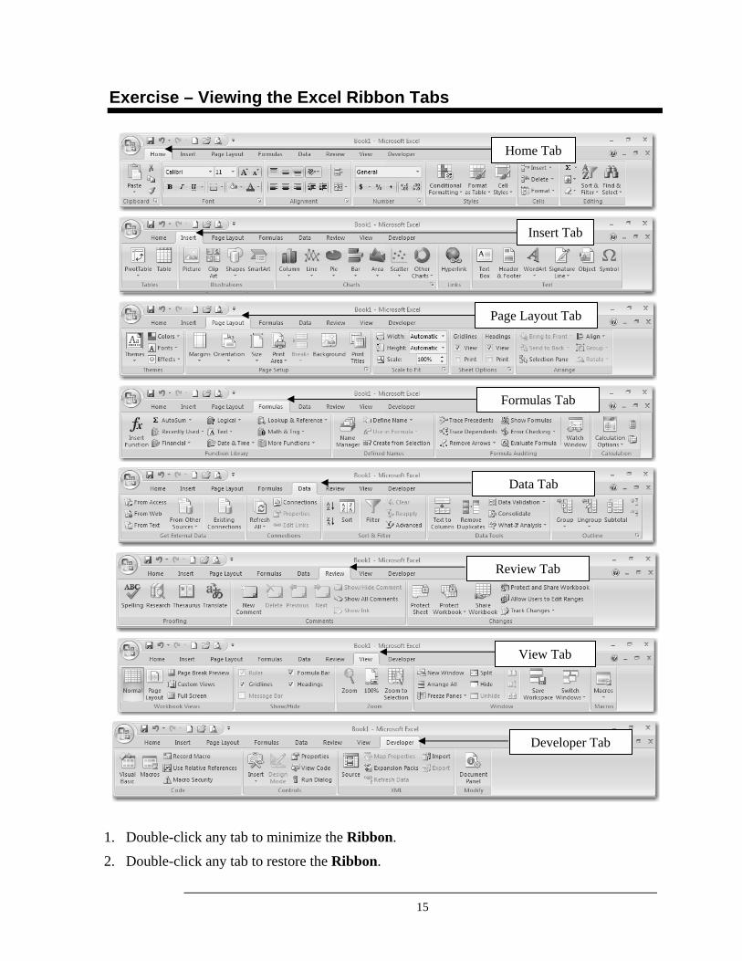
View the Excel Ribbon Tabs

The Ribbon replaces the traditional menus and toolbars found in earlier versions of Office. Tabs are used instead of menus. Commands are put in groups. Several galleries include a button to display a dialog box, which allows you to view additional options. The default display of the Ribbon includes all commands on all tabs being visible at all times. You can minimize the ribbon by double clicking a tab to hide the commands. The right-click option allows you to turn the Minimize the Ribbon feature on and off like a toggle switch from a list of choices. There are three basic components to the Ribbon: Tabs, Groups, and Commands There are seven main tabs across the top: Home, Insert, Page Layout, Formulas, Data, Review, and View. Each tab represents core tasks you do in excel. Each tab has groups that show related commands/features together. A command is a button, a menu, or a box to enter information. The Home tab is displayed by default when a new or existing workbook is opened. It includes clipboard commands such as cut, copy, and paste; text formatting commands such as font size, color, type; paragraph formatting commands such as text alignment, line spacing, borders and shading; and editing commands such as find and replace. The Insert tab includes commands for various items that are inserted into worksheets such as, tables, pictures, illustrations, links, headers and footers, text, and symbols. The Page Layout tab includes commands associated with the workbook themes, page setup and page background, and arranging objects within a worksheet. The Formulas tab includes commands associated with inserting formulas and functions into a worksheet. The Data tab includes the commands associated with importing data from external sources, sorting and filtering data using simple to complex criteria, grouping and ungrouping cell ranges, etc. The Review tab includes the proofing commands associated with spelling and grammar tools, thesaurus, language tools, etc.; comments, tracking changes, protecting and sharing worksheets and workbooks. The View tab includes commands associated with multiple ways of viewing your workbooks, showing and hiding the ruler and other tools; switching windows and viewing and recording macros. The Developer tab includes commands associated with creating and designing forms, macros and workbook security. This tab will not be discussed in this manual.

Ribbon

Minimize the Ribbon

Tabs

Groups Commands Home Tab

Insert Tab

Page Layout Tab

Formulas Tab

Data Tab

Review Tab

View Tab

Developer Tab

15

Exercise – Viewing the Excel Ribbon Tabs

1. Double-click any tab to minimize the Ribbon.

2. Double-click any tab to restore the Ribbon.

Page Layout Tab

Insert Tab

Home Tab

Formulas Tab

Data Tab

Review Tab

View Tab

Developer Tab

16

Moving Within a Worksheet

You may move the cell pointer to change the active cell with the mouse or by pressing keys on the keyboard. The Go To option on the Home tab in the Editing group on the Find & Select pull-down menu is also a way to move quickly to a specific cell in the worksheet.

Point at the cell you wish to make the active cell and click.

Click the Scroll Arrows to scroll one row or one column at a time. Click the Scroll Bar to scroll through the worksheet one screen at a time. Drag the Scroll Box along the scroll bar to move quickly through large sections of the worksheet at a time.

Press this key To get this cell

[Enter] or [Down Arrow] cell directly below (next row)

[Tab] or [Right Arrow] cell on right (next column)

[Up Arrow] cell directly above (previous row)

[Left Arrow] Cell on left (previous column)

[Ctrl+Home] Cell A1

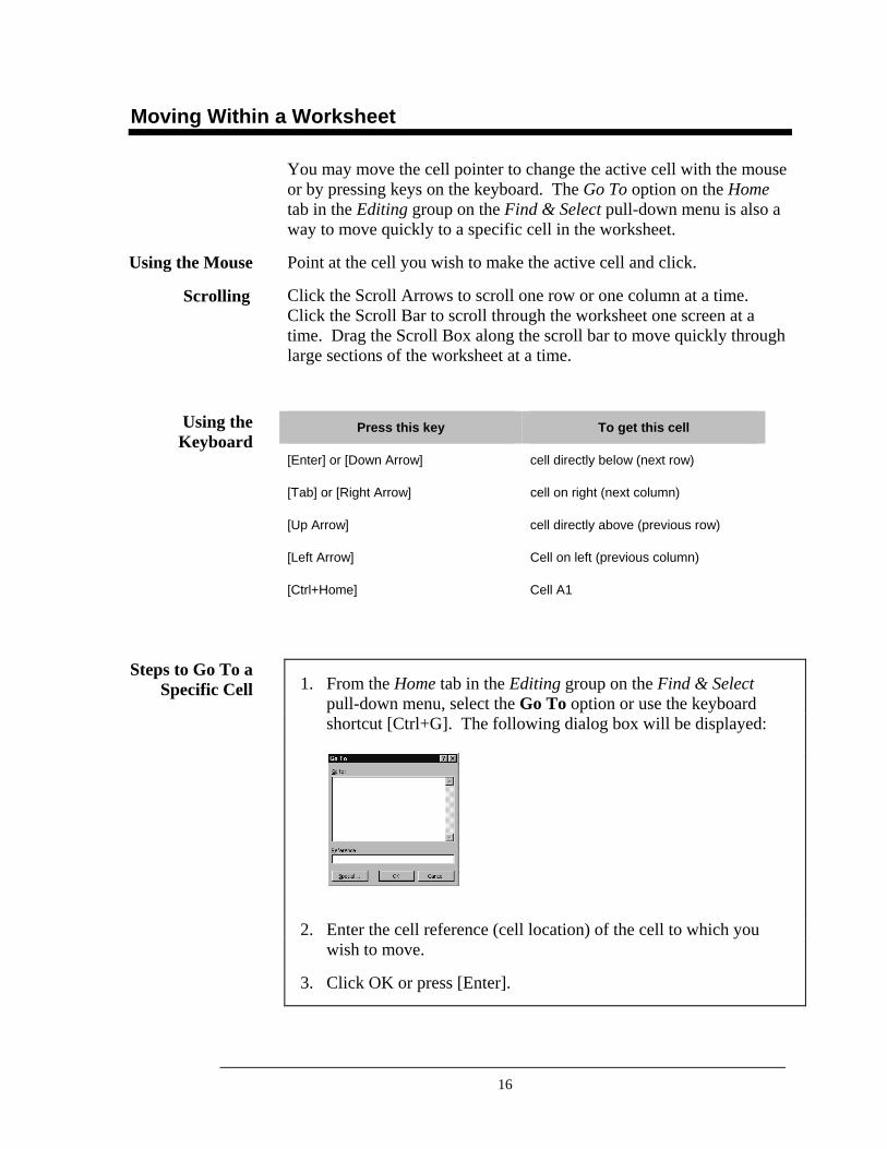
1. From the Home tab in the Editing group on the Find & Select pull-down menu, select the Go To option or use the keyboard shortcut [Ctrl+G]. The following dialog box will be displayed:

2. Enter the cell reference (cell location) of the cell to which you wish to move.

3. Click OK or press [Enter].

Using the Mouse

Scrolling

Using the Keyboard

Steps to Go To a Specific Cell

17

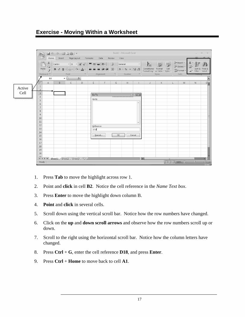
Exercise - Moving Within a Worksheet

1. Press Tab to move the highlight across row 1.

2. Point and click in cell B2. Notice the cell reference in the Name Text box.

3. Press Enter to move the highlight down column B.

4. Point and click in several cells.

5. Scroll down using the vertical scroll bar. Notice how the row numbers have changed.

6. Click on the up and down scroll arrows and observe how the row numbers scroll up or down.

7. Scroll to the right using the horizontal scroll bar. Notice how the column letters have changed.

8. Press Ctrl + G, enter the cell reference D18, and press Enter.

9. Press Ctrl + Home to move back to cell A1.

Active Cell

18

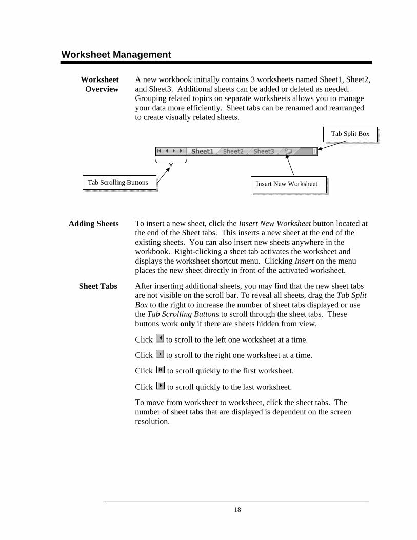
Worksheet Management

A new workbook initially contains 3 worksheets named Sheet1, Sheet2, and Sheet3. Additional sheets can be added or deleted as needed. Grouping related topics on separate worksheets allows you to manage your data more efficiently. Sheet tabs can be renamed and rearranged to create visually related sheets.

To insert a new sheet, click the Insert New Worksheet button located at the end of the Sheet tabs. This inserts a new sheet at the end of the existing sheets. You can also insert new sheets anywhere in the workbook. Right-clicking a sheet tab activates the worksheet and displays the worksheet shortcut menu. Clicking Insert on the menu places the new sheet directly in front of the activated worksheet.

After inserting additional sheets, you may find that the new sheet tabs are not visible on the scroll bar. To reveal all sheets, drag the Tab Split Box to the right to increase the number of sheet tabs displayed or use the Tab Scrolling Buttons to scroll through the sheet tabs. These buttons work only if there are sheets hidden from view.

Click to scroll to the left one worksheet at a time.

Click to scroll to the right one worksheet at a time.

Click to scroll quickly to the first worksheet.

Click to scroll quickly to the last worksheet.

To move from worksheet to worksheet, click the sheet tabs. The number of sheet tabs that are displayed is dependent on the screen resolution.

Worksheet Overview

Adding Sheets

Sheet Tabs

Tab Split Box

Tab Scrolling Buttons Insert New Worksheet

19

Exercise – Worksheet Management

1. Insert 6 new worksheets by clicking the Insert Worksheet button.

2. Practice clicking to scroll to the right one worksheet at a time.

3. Practice clicking to scroll to the left one worksheet at a time.

4. Click to scroll quickly to the last worksheet.

5. Click to scroll quickly to the first worksheet.

6. Drag the Tab Split Box to the right to increase the number of sheet tabs displayed until all sheets are displayed.

7. Activate Sheet9 by right-clicking to display the worksheet shortcut menu. Click Delete.

8. Click the Sheet6 tab. Hold down SHIFT while clicking the Sheet8 tab. Release the mouse and SHIFT key.

9. Right-click any sheet tab in the group to display the worksheet shortcut menu. Click Delete at the shortcut menu. We are back to the 5 sheets.

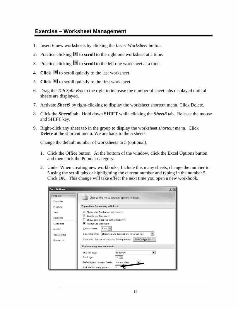
Change the default number of worksheets to 5 (optional). 1. Click the Office button. At the bottom of the window, click the Excel Options button

and then click the Popular category.

2. Under When creating new workbooks, Include this many sheets, change the number to 5 using the scroll tabs or highlighting the current number and typing in the number 5. Click OK. This change will take effect the next time you open a new workbook.

20

Hide or Unhide Worksheets

You can hide any worksheet in a workbook to remove it from view. You can also hide the workbook window of a workbook to remove it from your workspace. The data in hidden worksheets and workbook windows is not visible, but it can still be referenced from other worksheets and workbooks. You can display hidden worksheets or workbook windows as needed.

By default, all workbook windows of workbooks that you open are displayed on the taskbar, but you can hide or display them on the taskbar as needed.

To hide worksheets, you first need to select them. You have several options:

To Select Do This

A single sheet Click the sheet tab. If you don’t see the tab that you want, click the tab scrolling buttons to display the tab, and then click the tab.

Two or more adjacent sheets Click the tab for the first sheet. Then hold down SHIFT while you click the tab for the last sheet that you want to select.

Two or more nonadjacent sheets

Click the tab for the first sheet. Then hold down CTRL while you click the tabs of the other sheets that you want to select.

All sheets in a workbook Right-click a sheet tab, and then click Select All Sheets on the shortcut menu.

1. On the Home tab in the Cells group, click Format.

2. Under Visibility, click Hide & Unhide, and then click Hide Sheet.


2. Under Visibility, click Hide & Unhide, and then click Unhide Sheet.

3. In the Unhide sheet box, double-click the name of the hidden sheet that you want to display.

You can unhide only one worksheet at a time.

Invisible but not gone

Selecting Worksheets

Steps to Hide Worksheets

Steps to Unhide Worksheets

21

Exercise – Hide or Unhide Worksheets

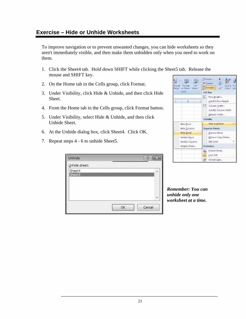
To improve navigation or to prevent unwanted changes, you can hide worksheets so they aren't immediately visible, and then make them unhidden only when you need to work on them. 1. Click the Sheet4 tab. Hold down SHIFT while clicking the Sheet5 tab. Release the

mouse and SHIFT key.


3. Under Visibility, click Hide & Unhide, and then click Hide Sheet.

4. From the Home tab in the Cells group, click Format button.

5. Under Visibility, select Hide & Unhide, and then click Unhide Sheet.

6. At the Unhide dialog box, click Sheet4. Click OK.

7. Repeat steps 4 - 6 to unhide Sheet5.

Remember: You can unhide only one worksheet at a time.

22

Rename/Rearrange Worksheets

The Sheet Tabs at the bottom of the screen are used to move from worksheet to worksheet within the workbook. You may change the default sheet names (Sheet1, Sheet2...) in order to give them more meaningful names.

To change the name of a Sheet Tab, double-click the Sheet Tab. It will select the name of the sheet. Type the new name and then press Enter. Sheet names can be up to 31 characters in length and may include spaces.

1. Double-click the Sheet Tab you wish to rename.

2. When the sheet name is selected, type the new name. The name may contain up to 31 characters and can also include spaces.

Sheet Tabs may be dragged to rearrange the order of the worksheets within the workbook. To move a worksheet in front of another worksheet, click and drag the Sheet Tab you wish to move between the tabs of its final location.

1. Select the Sheet Tab you wish to move.

2. Click and drag the Sheet Tab you wish to move between the tabs of its final location.

When you are moving a sheet, an arrow will appear to show you where the sheet will move to when you release the mouse button.

Name Sheet Tabs

Steps to Rename Sheet

Steps to Rearrange

Sheets

Tip

23

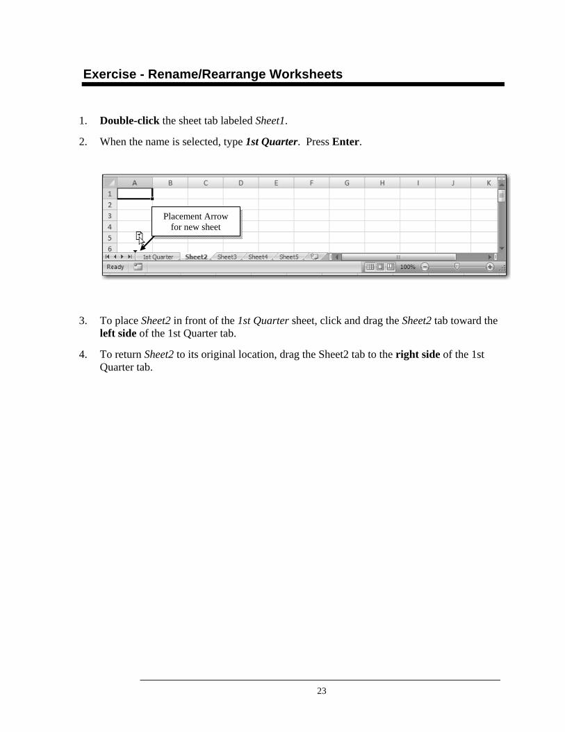
Exercise - Rename/Rearrange Worksheets

1. Double-click the sheet tab labeled Sheet1.

2. When the name is selected, type 1st Quarter. Press Enter.

3. To place Sheet2 in front of the 1st Quarter sheet, click and drag the Sheet2 tab toward the left side of the 1st Quarter tab.

4. To return Sheet2 to its original location, drag the Sheet2 tab to the right side of the 1st Quarter tab.

Placement Arrow for new sheet

24

Color Code Worksheet Tabs

Changing the color of sheet tabs can help to visually identify related worksheets or can be used to show how the workbook is organized. This way, when opening a workbook that has many worksheets, you can visually identify related sheets by color coding them with the same color scheme. The active worksheet tab displays white with the tab name underlined with the selected color. Inactive worksheets display the full color selected.

1. Right-click the worksheet tab you want to color.

2. From the short-menu, select Tab Color.

3. Select a color by clicking on a color box.

4. Click a different worksheet tab in order to see the full color added to the worksheet tab.

Organize by Color

Active Worksheet

Steps to Color Code Worksheet

Tabs

25

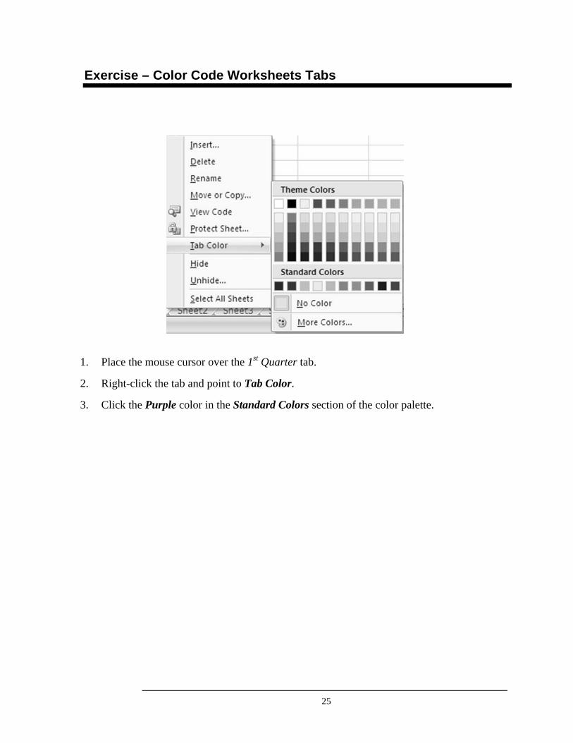
Exercise – Color Code Worksheets Tabs

1. Place the mouse cursor over the 1st Quarter tab.

2. Right-click the tab and point to Tab Color.

3. Click the Purple color in the Standard Colors section of the color palette.

26

Enter Text into Cells

To enter information into a worksheet, select a cell and begin typing. The cell contents will display in the formula bar as you type. To place the contents into the cell, press either the [Enter] key or the [Tab] key. If the [Tab] key is pressed, the information will be entered into the active cell and the cursor will automatically advance to the cell on the right (in the next column). If the [Enter] key is pressed, the information will be entered into the active cell and the cursor will automatically advance to the cell below (in the next row).

If the contents of a cell are alphanumeric (letters or a combination of letters and numbers), Excel will treat the entry as text. By default, text entries are left aligned. If numbers are included with text, Excel regards that entire entry as text. For example, a flight number TWA123 is considered text due to the nonnumeric characters included. Excel will interpret anything with nonnumeric characters as text.

Text used as a heading for a row or column is referred to as a label. Labels should be descriptive, and thus are often longer than the width of a cell. If there is a blank cell to the right of the label cell, Excel “spills over” the contents of the cell into the adjacent cell. If the adjacent cell is not blank, Excel will only display as much of the label as will fit into the cell. The rest of the cell entry is still there even though it is not visible, and it will be redisplayed if you change the width of the column. Changing column width will be discussed later.

1. Select a cell and type the information.

2. Press [Enter] to enter the contents into the cell and advance the cursor to the cell below. OR Press [Tab] to enter the contents into the cell and advance the cursor to the cell to the right.

Entering Information into

Cells

Entering Text

Labels

Steps to Enter Data into Cells

27

Exercise - Enter Text into Cells

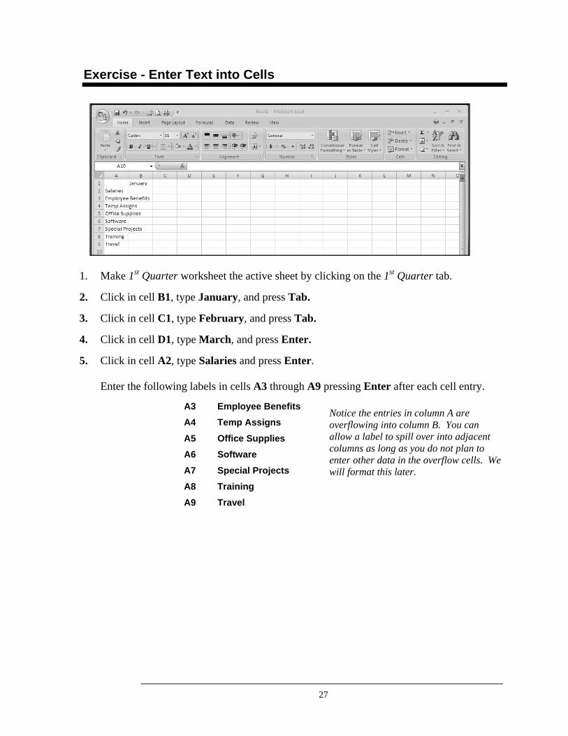
1. Make 1st Quarter worksheet the active sheet by clicking on the 1st Quarter tab.

2. Click in cell B1, type January, and press Tab.

3. Click in cell C1, type February, and press Tab.

4. Click in cell D1, type March, and press Enter.

5. Click in cell A2, type Salaries and press Enter. Enter the following labels in cells A3 through A9 pressing Enter after each cell entry.

A3 Employee Benefits A4 Temp Assigns A5 Office Supplies A6 Software A7 Special Projects A8 Training A9 Travel

Notice the entries in column A are overflowing into column B. You can allow a label to spill over into adjacent columns as long as you do not plan to enter other data in the overflow cells. We will format this later.

28

Enter Numbers into Cells

If the contents of a cell are numeric, the contents will be right aligned. When entering numbers in a worksheet, type only the integers and decimals. Do not type commas, dollar signs, or percent signs. You will learn later how to add commas, dollar signs, and percent signs by formatting the cell contents. If the number is negative, type a minus sign before the number or enclose the number in parentheses.

If numbers are being entered as text, for example a zip code or a social security number, without any nonnumeric characters, the text numbers must be preceded by an apostrophe or the format may be changed to text after entering the data. The apostrophe tells Excel that the number is actually text and is not to be used in any type of calculations. The text number entry will also be left aligned rather than the standard right-alignment that Excel uses for numbers.

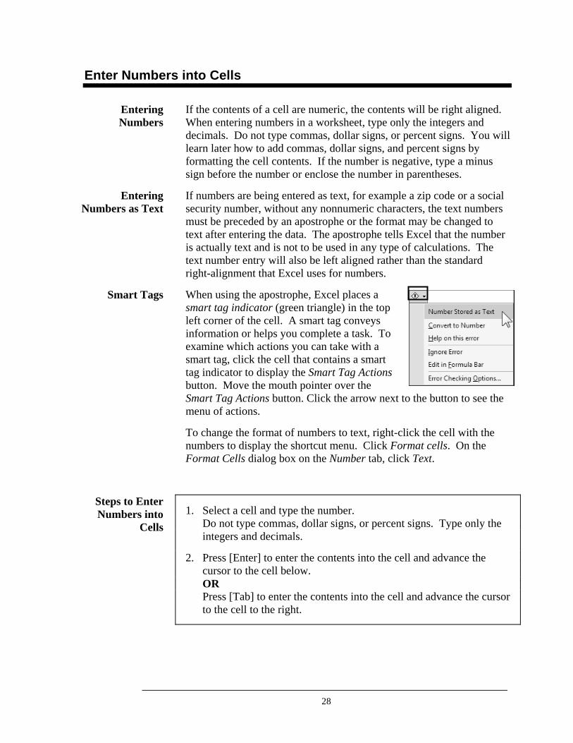
When using the apostrophe, Excel places a smart tag indicator (green triangle) in the top left corner of the cell. A smart tag conveys information or helps you complete a task. To examine which actions you can take with a smart tag, click the cell that contains a smart tag indicator to display the Smart Tag Actions button. Move the mouth pointer over the Smart Tag Actions button. Click the arrow next to the button to see the menu of actions.

To change the format of numbers to text, right-click the cell with the numbers to display the shortcut menu. Click Format cells. On the Format Cells dialog box on the Number tab, click Text.

1. Select a cell and type the number. Do not type commas, dollar signs, or percent signs. Type only the integers and decimals.

2. Press [Enter] to enter the contents into the cell and advance the cursor to the cell below. OR Press [Tab] to enter the contents into the cell and advance the cursor to the cell to the right.

Entering Numbers

Entering Numbers as Text

Smart Tags

Steps to Enter Numbers into

Cells

29

Exercise - Enter Numbers into Cells

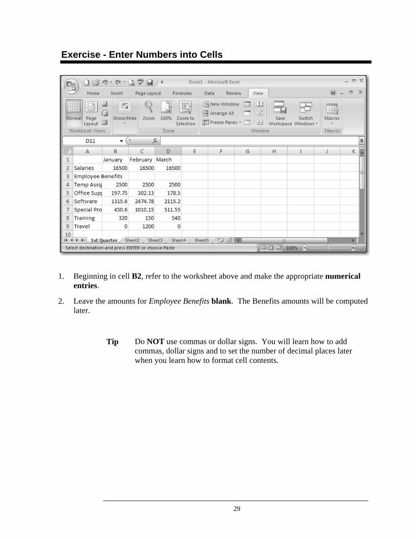
1. Beginning in cell B2, refer to the worksheet above and make the appropriate numerical

entries.

2. Leave the amounts for Employee Benefits blank. The Benefits amounts will be computed later.

Do NOT use commas or dollar signs. You will learn how to add commas, dollar signs and to set the number of decimal places later when you learn how to format cell contents.

Tip

30

Save a Workbook

To avoid the accidental loss of data, you should save your work often. There are two options for saving, Save and Save As. The Save command is used for a first-time save or if you have made revisions to a workbook and wish to replace the old version with your new revised workbook. When the Save command is selected and it is a first-time save, a dialog box will be displayed. In this dialog box, a name must be given to the workbook and a folder must be designated as the location in which to save the workbook. The dialog box will not be displayed if it is not a first-time save.

1. From the Office button, select the Save command or click the Save

icon on the Quick Access toolbar.

2. In the Save As dialog box, type a name for the workbook. Filenames can contain up to 255 alphanumeric characters including space. They cannot include: \ ? : * “ < > /.

3. Verify that you are saving to the proper drive and folder. If not, make changes: To change the drive, click Computer in the Folders list and double-click the correct drive. To change the folder, double-click on the icon for the correct folder. To create a new folder, click the New Folder button.

4. Click the Save button.

After making revisions to a workbook, you may choose Save As and give the workbook a new name to save a different version of the workbook in addition to the original. There are several Save As options with Excel 2007.

Saving Options

Steps to Save a Workbook

Save As Options

31

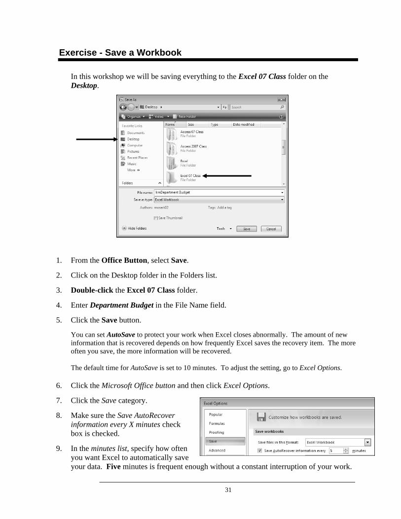
Exercise - Save a Workbook

In this workshop we will be saving everything to the Excel 07 Class folder on the Desktop.

1. From the Office Button, select Save.

2. Click on the Desktop folder in the Folders list.

3. Double-click the Excel 07 Class folder.

4. Enter Department Budget in the File Name field.

5. Click the Save button.

You can set AutoSave to protect your work when Excel closes abnormally. The amount of new information that is recovered depends on how frequently Excel saves the recovery item. The more often you save, the more information will be recovered. The default time for AutoSave is set to 10 minutes. To adjust the setting, go to Excel Options.

6. Click the Microsoft Office button and then click Excel Options.

7. Click the Save category.

8. Make sure the Save AutoRecover information every X minutes check box is checked.

9. In the minutes list, specify how often you want Excel to automatically save your data. Five minutes is frequent enough without a constant interruption of your work.

32

Select Cells

Any time cell contents need to be formatted or edited, the cells to be changed must be selected first. It is possible to select a single cell, an entire row or column, a block of cells, or all the cells in a worksheet. The selected cells will be highlighted on the screen.

In a worksheet a block of two or more cells is referred to as a range. The range reference includes the first and last cell in the range separated by a colon (:). For example, the range of cells from, and including, A1 to D9 is written as A1:D9.

The following is a summary of Excel selection methods.

Selection Method Action

Cell Range Position the mouse pointer in the first cell of the selection. Then hold the left mouse button down as you drag diagonally to the end of the block of cells to be selected, release the mouse button.

OR

Click the first cell of the range. Using the scroll bars and arrows, scroll to the end of the range. Hold down the [Shift] key as you click the last cell of the range.

Row(s) Click the row heading (number) to select an entire row.

To select multiple rows, drag the mouse pointer through the row headings.

Column(s) Click the column heading (letter) to select an entire column.

To select multiple columns, drag the mouse pointer through the column headings.

Nonadjacent Cells or Ranges

Hold down the [Ctrl] key as you click individual cells or drag through ranges of cells.

Entire Worksheet Press the keyboard shortcut, [Ctrl] +A, or click the Select All button located just above the row headings and to the left of the column headings (see screen print on next page). Select All is useful for formatting changes to the entire worksheet, such as changing the font for the entire worksheet.

Deselect Click anywhere on your worksheet.

Why Select Cells?

Selection Methods:

33

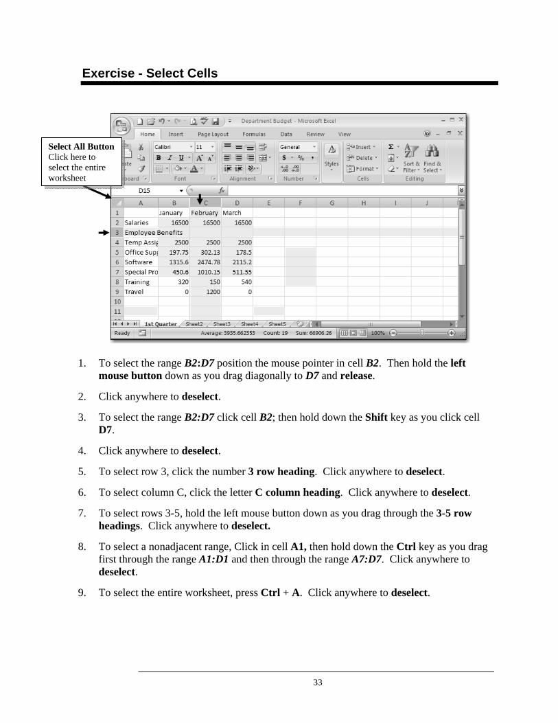
Exercise - Select Cells

1. To select the range B2:D7 position the mouse pointer in cell B2. Then hold the left mouse button down as you drag diagonally to D7 and release.

2. Click anywhere to deselect.

3. To select the range B2:D7 click cell B2; then hold down the Shift key as you click cell D7.


5. To select row 3, click the number 3 row heading. Click anywhere to deselect.

6. To select column C, click the letter C column heading. Click anywhere to deselect.

7. To select rows 3-5, hold the left mouse button down as you drag through the 3-5 row headings. Click anywhere to deselect.

8. To select a nonadjacent range, Click in cell A1, then hold down the Ctrl key as you drag first through the range A1:D1 and then through the range A7:D7. Click anywhere to deselect.

9. To select the entire worksheet, press Ctrl + A. Click anywhere to deselect.

Select All Button Click here to select the entire worksheet

34

Change Column Width & Row Height

When the contents of a cell are longer than the width of the cell, the cell’s contents will “spill” over into the cell to the immediate right. If the cell to the immediate right is empty, the overflow will be displayed in that cell. If the cell to the immediate right contains an entry, the overflow will be truncated. It will appear as if the overflowing text has been cut off. In order to redisplay the hidden contents, you will need to expand the column width.

Another occasion that columns will need to be widened is when #### signs or scientific notations (7.89e+06) are displayed in a cell. This happens when formatted numbers do not fit within the width of a cell. Excel will store the complete information, but it does not have enough room to display it. To fully display the formatted numeric information, it is necessary to widen the column.

1. For the column to be widened, position the pointer on the vertical line at the right side of the column heading until the pointer changes

to (see screen print on next page).

2. Press and drag until the column is the desired width. OR Double-click to automatically (Best Fit) widen the column to accommodate the widest entry.

Row height can also be adjusted in Excel to improve readability or to provide emphasis to information in particular rows.

1. Position the pointer on the gridline below the row number for the row to be heightened until the pointer changes to (see screen print on next page).

2. Press and drag until the row is the desired height. OR Double-click to automatically adjust (Best Fit) the height of the row to accommodate the row contents.

It is possible to increase the width of several columns at once or to increase the height of several rows at once if you select all the columns or all the rows before dragging.

Cell Spill Over

Symbols That Don't Make

Sense!

Steps to Change Column Width

Steps to Change Row Height

Tip

35

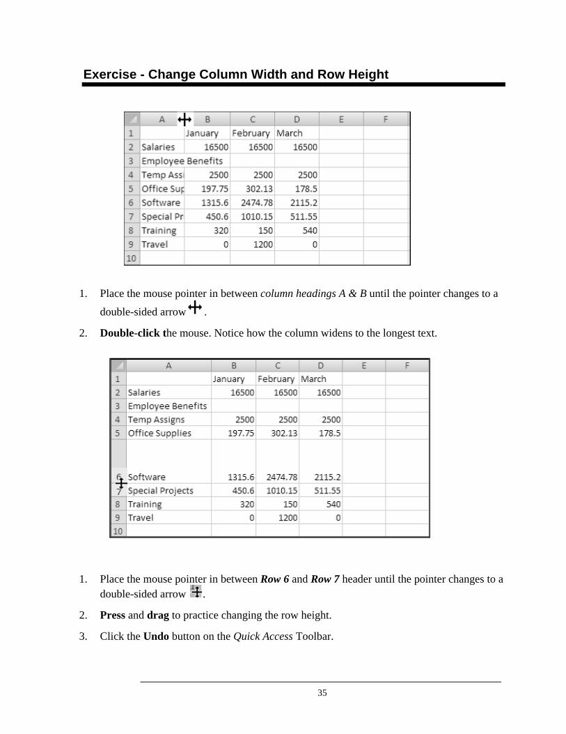
Exercise - Change Column Width and Row Height

1. Place the mouse pointer in between column headings A & B until the pointer changes to a

double-sided arrow .

2. Double-click the mouse. Notice how the column widens to the longest text.

1. Place the mouse pointer in between Row 6 and Row 7 header until the pointer changes to a

double-sided arrow .

2. Press and drag to practice changing the row height.

3. Click the Undo button on the Quick Access Toolbar.

36

Edit Cell Contents

The contents of a cell may be edited to update data or to correct a mistake. One way is to select the cell and retype the entry. When you press [Enter] the new entry will replace the old cell contents.

Another way is to select the cell and insert and/or delete characters within the entry. To do this, select the cell you wish to edit. The cell contents will be displayed in the formula bar. Click the editing I-Beam to position the cursor within the text in the formula bar and insert or delete characters as necessary. When you are finished editing the entry, press [Enter] to place the entry in the cell. If you prefer to edit within the cell rather than in the formula bar, double-click the cell to activate Edit Mode.

1. Select the cell to be edited.

2. Type the new entry. The old entry will erase as soon as you begin typing. OR Click the I-Beam within the cell contents in the formula bar and then make the necessary changes. OR Double-click the cell to activate Edit mode. Insert or delete text as necessary.

3. Press [Enter] to place the new cell contents into the cell.

If you make a mistake or change your mind while editing or formatting a worksheet, you may click the Undo button. The Undo button will reverse the last action you took.

When entering data into a cell or editing data, the data is displayed in the formula bar along with buttons that may be clicked to cancel the entry if you change your mind or enter the data into the cell (see screen print on next page).

Edit Cell Contents

Undo Button

Important

37

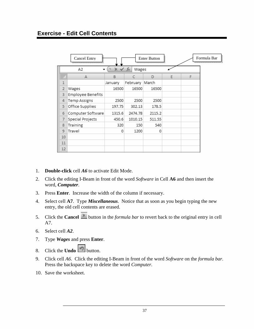
Exercise - Edit Cell Contents

1. Double-click cell A6 to activate Edit Mode.

2. Click the editing I-Beam in front of the word Software in Cell A6 and then insert the word, Computer.

3. Press Enter. Increase the width of the column if necessary.

4. Select cell A7. Type Miscellaneous. Notice that as soon as you begin typing the new entry, the old cell contents are erased.

5. Click the Cancel button in the formula bar to revert back to the original entry in cell A7.

6. Select cell A2.

7. Type Wages and press Enter.

8. Click the Undo button.

9. Click cell A6. Click the editing I-Beam in front of the word Software on the formula bar. Press the backspace key to delete the word Computer.

10. Save the worksheet.

Cancel Entry Enter Button Formula Bar

38

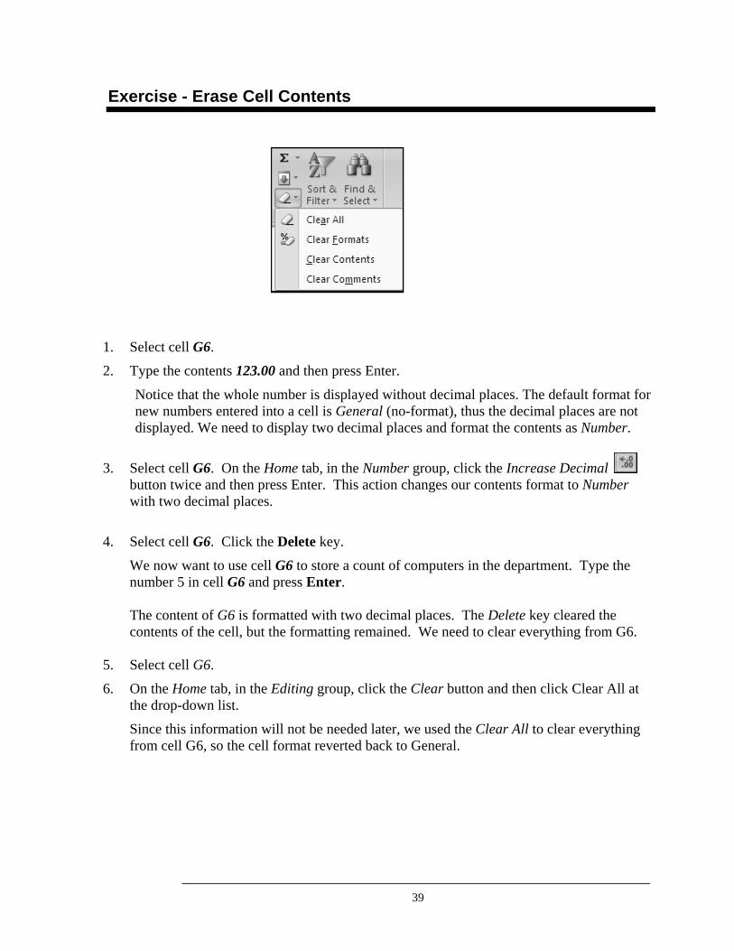
Erase Cell Contents

You can clear cells to remove the cell contents (formulas and data), formats (including number formats, conditional formats, and borders), and any attached comments. The cleared cells remain as blank or unformatted cells on the worksheet.

On the Home tab, in the Editing group, click the Clear button.

A drop-down menu is displayed showing the Clear options:

Clear Options Description

Clear All Clears all contents, formats, and comments that are contained in the selected cells.

Clear Formats Formats are cleared while contents remain in the selected cells.

Clear Contents The contents in the selected cells are cleared, leaving any formats and comments in place.

Clear Comments Clears any comments that are attached to selected cells.

You can also select the cell or range of cells and press Delete on the keyboard. Delete or Backspace clears only the contents of the cell; formats or comments applied to the cell remain in effect.

1. Select the cell or range of cells to be erased.

2. On the Home tab, in the Editing group, click the arrow next to the Clear button. A pull-down submenu will be displayed.

3. Click your selection.

If you want to remove cells from the worksheet and shift the surrounding cells to fill the space, select the cells and delete them. On the Home tab, in the Cells group, click the arrow next to Delete, and then click Delete Cells.

Steps to Erase Cell Contents

Tip

39

Exercise - Erase Cell Contents

1. Select cell G6.

2. Type the contents 123.00 and then press Enter.

Notice that the whole number is displayed without decimal places. The default format for new numbers entered into a cell is General (no-format), thus the decimal places are not displayed. We need to display two decimal places and format the contents as Number.

3. Select cell G6. On the Home tab, in the Number group, click the Increase Decimal button twice and then press Enter. This action changes our contents format to Number with two decimal places.

4. Select cell G6. Click the Delete key.

We now want to use cell G6 to store a count of computers in the department. Type the number 5 in cell G6 and press Enter. The content of G6 is formatted with two decimal places. The Delete key cleared the contents of the cell, but the formatting remained. We need to clear everything from G6.

5. Select cell G6.

6. On the Home tab, in the Editing group, click the Clear button and then click Clear All at the drop-down list.

Since this information will not be needed later, we used the Clear All to clear everything from cell G6, so the cell format reverted back to General.

40

Formulas

Formulas are equations that perform calculations on values in your worksheet. All formulas in Excel begin with the equal sign (=) as the first character. Formulas can include operators, cell references, constant values, and functions. (Functions will be discussed later.)

Operators specify the type of calculation that you want to perform on the elements of a formula. There are four types of operators: arithmetic, comparison, text concatenation, and reference.

Arithmetic operators perform basic mathematical operations such as addition, subtraction, multiplication, division, exponentiation, negation, and calculating percentages.

Comparison operators allow you to compare two values. The result is a logical value either TRUE or FALSE.

= Equal to

<> Not equal to

> Greater than

< Less than

>= Greater than or equal to

<= Less than or equal to

Use the ampersand (&) to join, or concatenate, two or more text strings to produce a single piece of text. For example, “North”&“wind” results in Northwind Combine ranges of cells for calculations with reference operators.

Operators

Arithmetic Operators

Comparison Operators

Concatenation Operators

Reference Operators

Reference Operator

Description Example

Colon (:) Range operator which produces one reference to all the cells between two references, including the two references.

B5:B15

Comma(,) Union operator, which combines multiple references into one reference.

SUM(B5:B15,D5:D9)

Space Intersection operator which produces one reference to cells common to the two references

B7:D7 C6:C8 C7

41

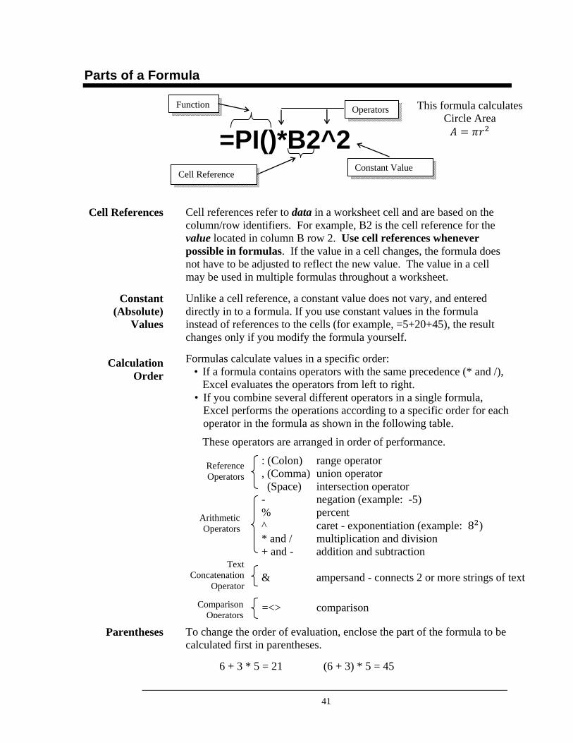
Parts of a Formula

=PI()*B2^2

Cell references refer to data in a worksheet cell and are based on the column/row identifiers. For example, B2 is the cell reference for the value located in column B row 2. Use cell references whenever possible in formulas. If the value in a cell changes, the formula does not have to be adjusted to reflect the new value. The value in a cell may be used in multiple formulas throughout a worksheet.

Unlike a cell reference, a constant value does not vary, and entered directly in to a formula. If you use constant values in the formula instead of references to the cells (for example, =5+20+45), the result changes only if you modify the formula yourself.

Formulas calculate values in a specific order: • If a formula contains operators with the same precedence (* and /),

Excel evaluates the operators from left to right. • If you combine several different operators in a single formula,

Excel performs the operations according to a specific order for each operator in the formula as shown in the following table.

These operators are arranged in order of performance.

: (Colon) range operator , (Comma) union operator (Space) intersection operator - negation (example: -5) % percent ^ caret - exponentiation (example: 8 ) * and / multiplication and division + and - addition and subtraction & ampersand - connects 2 or more strings of text =<> comparison

To change the order of evaluation, enclose the part of the formula to be calculated first in parentheses.

6 + 3 * 5 = 21 (6 + 3) * 5 = 45

Cell References

Constant (Absolute)

Values

Calculation Order

Parentheses

Function

Cell Reference Constant Value

Operators

This formula calculates Circle Area

Arithmetic Operators

Reference Operators

Text Concatenation

Operator

Comparison Operators

42

Creating Formulas

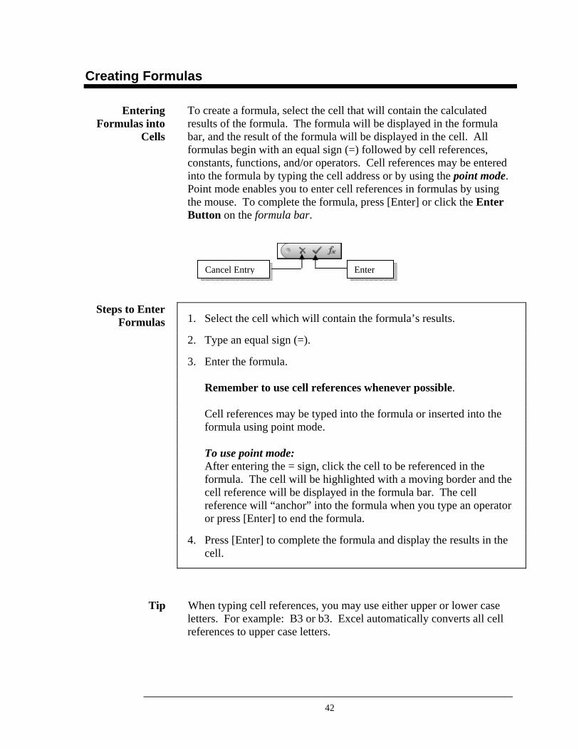
To create a formula, select the cell that will contain the calculated results of the formula. The formula will be displayed in the formula bar, and the result of the formula will be displayed in the cell. All formulas begin with an equal sign (=) followed by cell references, constants, functions, and/or operators. Cell references may be entered into the formula by typing the cell address or by using the point mode. Point mode enables you to enter cell references in formulas by using the mouse. To complete the formula, press [Enter] or click the Enter Button on the formula bar.

1. Select the cell which will contain the formula’s results.

2. Type an equal sign (=).

3. Enter the formula. Remember to use cell references whenever possible. Cell references may be typed into the formula or inserted into the formula using point mode. To use point mode: After entering the = sign, click the cell to be referenced in the formula. The cell will be highlighted with a moving border and the cell reference will be displayed in the formula bar. The cell reference will “anchor” into the formula when you type an operator or press [Enter] to end the formula.

4. Press [Enter] to complete the formula and display the results in the cell.

When typing cell references, you may use either upper or lower case letters. For example: B3 or b3. Excel automatically converts all cell references to upper case letters.

Entering Formulas into

Cells

Steps to Enter Formulas

Tip

Cancel Entry Enter

43

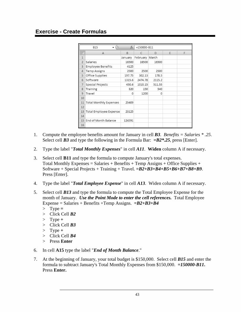
Exercise - Create Formulas

1. Compute the employee benefits amount for January in cell B3. Benefits = Salaries * .25. Select cell B3 and type the following in the Formula Bar: =B2*.25, press [Enter].

2. Type the label "Total Monthly Expenses" in cell A11. Widen column A if necessary.

3. Select cell B11 and type the formula to compute January's total expenses. Total Monthly Expenses = Salaries + Benefits + Temp Assigns + Office Supplies + Software + Special Projects + Training + Travel. =B2+B3+B4+B5+B6+B7+B8+B9. Press [Enter].

4. Type the label "Total Employee Expense" in cell A13. Widen column A if necessary.

5. Select cell B13 and type the formula to compute the Total Employee Expense for the month of January. Use the Point Mode to enter the cell references. Total Employee Expense = Salaries + Benefits +Temp Assigns. =B2+B3+B4 > Type = > Click Cell B2 > Type + > Click Cell B3 > Type + > Click Cell B4 > Press Enter

6. In cell A15 type the label "End of Month Balance."

7. At the beginning of January, your total budget is $150,000. Select cell B15 and enter the formula to subtract January's Total Monthly Expenses from $150,000. =150000-B11. Press Enter.

44

Functions

You could accomplish every calculation that you wish to perform using formulas. For example, if you have constructed a spreadsheet with 100 rows and you wish to have one column of numbers added; you could build a formula that would do this by typing each of the 100 cell references along with numerous plus (+) signs. This is time consuming and tedious although effective. A more efficient way is to use a function.

Functions are predefined formula shortcuts that perform common worksheet calculations such as adding a row or column of numbers (SUM) or finding the average of the values in a range of cells (AVERAGE).

For example, you could use the formula, =B2+B3+B4+B5+B6+B7+B8+B9 to find the total expenses for January as you did in the previous exercise or... you could use the SUM function to give you the same results as the long formula of adding each cell. Using the SUM function to calculate the total expenses for January would be written as:

=SUM(B2:B9)

A function is composed of the function name followed by the argument(s) (values upon which a function operates) enclosed in parentheses. Arguments can be a combination of numerals, other functions, cell references, or ranges. A function can contain one, none, or several arguments. If more than one argument is used, they are separated by a comma.

To type a range in a formula, type the beginning cell reference of the range followed by a colon (:) and the ending cell reference. For example, a range is entered as B2:B7.

Using Calculations

What are Functions?

Arguments

Ranges

45

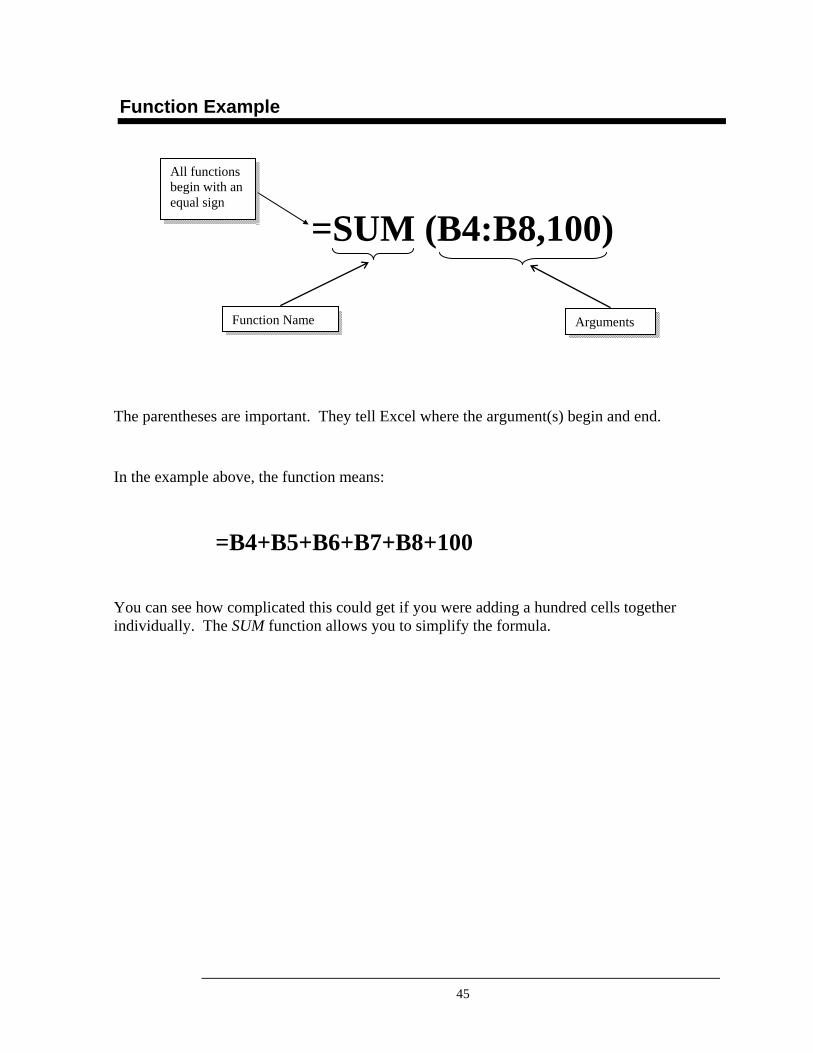
Function Example

=SUM (B4:B8,100)

The parentheses are important. They tell Excel where the argument(s) begin and end.

In the example above, the function means:

=B4+B5+B6+B7+B8+100

You can see how complicated this could get if you were adding a hundred cells together individually. The SUM function allows you to simplify the formula.

Function Name Arguments

All functions begin with an equal sign

46

Create Functions

Functions can be entered in a number of ways. Two ways are listed here, while the Function Wizard option is covered in the next section.

When typing a function, an equal (=) sign must be typed first – as with a formula. However, when using the AutoSum tool on the Home tab in the Editing group, the equal sign will be entered for you along with the SUM function name. Excel will guess at the cells that you want to SUM. If the cells are not correctly selected, you can use your mouse pointer to select the correct cells.

1. Select the cell that is to contain the results of the function.

2. Enter an equal sign, the function name, and a left parenthesis.

3. Enter the arguments by typing the cell references or cell ranges or by using the point mode. If more than one argument is used, separate them with a comma.

4. Enter the right parenthesis.

5. Press [Enter].

1. Select the cell that is to contain the results of the function. No need to enter the equal sign since the button will do it for you.

2. Click the AutoSum button on the Home tab in the Editing group. Excel makes its best guess and enters an argument. (50-50 chance it will be correct!)

3. If Excel’s guess is wrong, enter the correct argument(s) or use the point mode to select the correct cells.

4. Press [Enter].

The row and column headings are the number and letter cells on the left and top of worksheet. For the active cell(s) the row and column headings will be bolded.

Steps to Entering Functions by

Typing

Steps to Using the AutoSum

Button

Tip

47

Exercise - Creating Functions

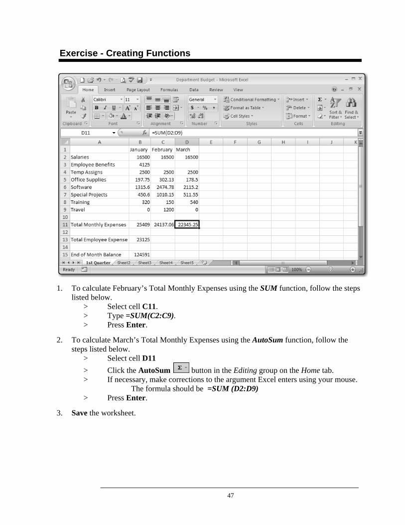
1. To calculate February’s Total Monthly Expenses using the SUM function, follow the steps listed below. > Select cell C11. > Type =SUM(C2:C9). > Press Enter.

2. To calculate March’s Total Monthly Expenses using the AutoSum function, follow the steps listed below. > Select cell D11 > Click the AutoSum button in the Editing group on the Home tab. > If necessary, make corrections to the argument Excel enters using your mouse. The formula should be =SUM (D2:D9) > Press Enter.


48

Insert Functions

There are a number of functions available in Excel. The Insert Function command allows you to choose the function you want from a list. This method is helpful when you are not sure of the exact name or format of the function you need to use.

To access the Insert Function options, click the Insert Function button

in the formula toolbar. The Insert Function dialog box will display. You can search for a function by typing in a description of what you want to do. Alternatively, you can select a category – or logical grouping – of functions. Selecting a category enables Excel to limit the search for the correct function. The Select a function section lists the functions available for the selected category. When a function is selected, a description of the calculation the function performs will be displayed beneath the Select a function window.

When using the Insert Function option, it is not necessary to type the equals sign first. The Insert Function command will do it for you.

1. Select the cell that you want to contain the results of the function.

2. Click the Insert Function button on the formula toolbar. The Insert Function dialog box will be displayed.

3. If the category is known, click it. If not, it is always safe to click ALL.

4. Scroll through the list of function names and select the desired function.

5. Click OK to display the Function Arguments dialog box.

6. Enter the argument(s).

7. Click OK.

Insert Function Command

Steps to Using the Insert Function

Command

49

Exercise – Inserting Functions

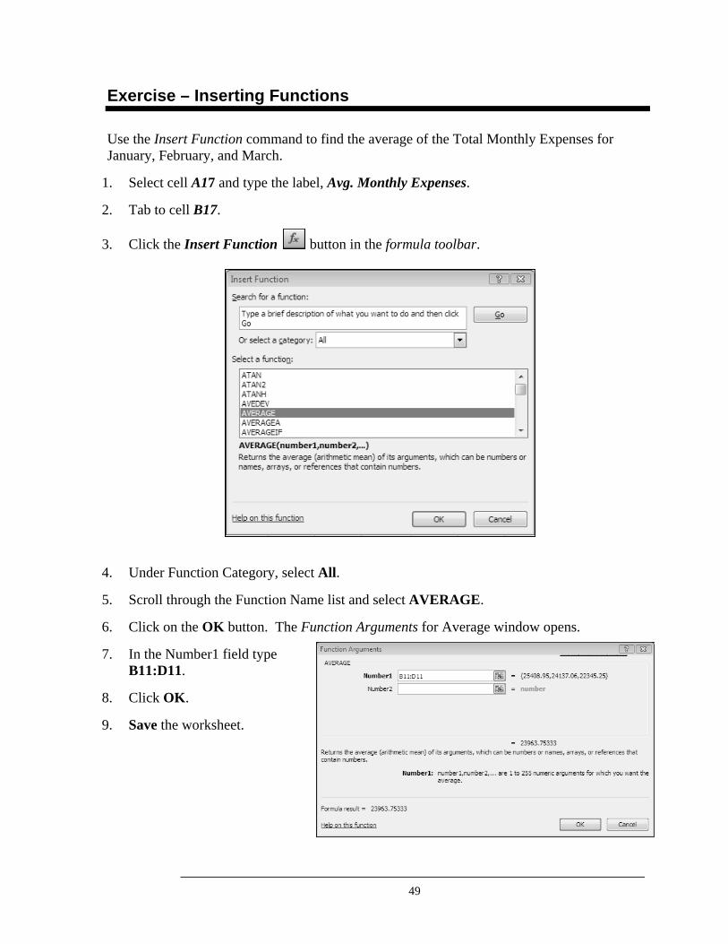
Use the Insert Function command to find the average of the Total Monthly Expenses for January, February, and March.

1. Select cell A17 and type the label, Avg. Monthly Expenses.

2. Tab to cell B17.

3. Click the Insert Function button in the formula toolbar.

4. Under Function Category, select All.

5. Scroll through the Function Name list and select AVERAGE.

6. Click on the OK button. The Function Arguments for Average window opens.

7. In the Number1 field type B11:D11.

8. Click OK.


50

Copy Formulas (Fill Command)

Formulas can be copied to other cells in order to simplify editing tasks and to expedite the building of a worksheet. Copying can be done via the Copy and Paste options on the Home tab in the Clipboard group, via the Fill command on the Home tab in the Editing group, or by using the worksheet Fill Handle.

In many cases you may create a worksheet in which several formulas are basically the same. For example, the formula to calculate the total monthly expenses for February, =SUM(C2:C9), is the same as the formula to calculate total monthly expenses for March, =SUM(D2:D9). The only difference between the two formulas is the column reference.

When formulas are copied, the cell containing the original formula is the source, and the cell(s) to which the formula is copied is called the destination. Excel uses relative references to automatically update the formula relative to the destination.

The relationship between the source cell and the reference cells is included in the formula. When the formula is copied to another cell, the relationship is also copied, and updated relative to the destination cell.

1. Select the destination cell.

2. On the Home tab in the Editing group, click the drop-down menu on

the Fill command button.

3. Click one of the choices on the short menu; Down, Right, Up, or Left.

Copying Formulas

Relative References

Steps to Use the Fill Options

51

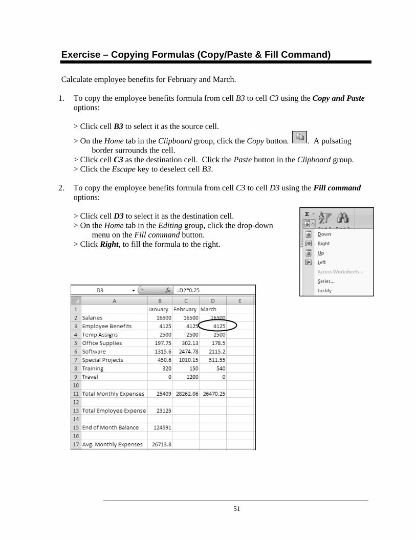
Exercise – Copying Formulas (Copy/Paste & Fill Command)

Calculate employee benefits for February and March.

1. To copy the employee benefits formula from cell B3 to cell C3 using the Copy and Paste options: > Click cell B3 to select it as the source cell.

> On the Home tab in the Clipboard group, click the Copy button. . A pulsating border surrounds the cell. > Click cell C3 as the destination cell. Click the Paste button in the Clipboard group. > Click the Escape key to deselect cell B3.

2. To copy the employee benefits formula from cell C3 to cell D3 using the Fill command options: > Click cell D3 to select it as the destination cell. > On the Home tab in the Editing group, click the drop-down menu on the Fill command button. > Click Right, to fill the formula to the right.

52

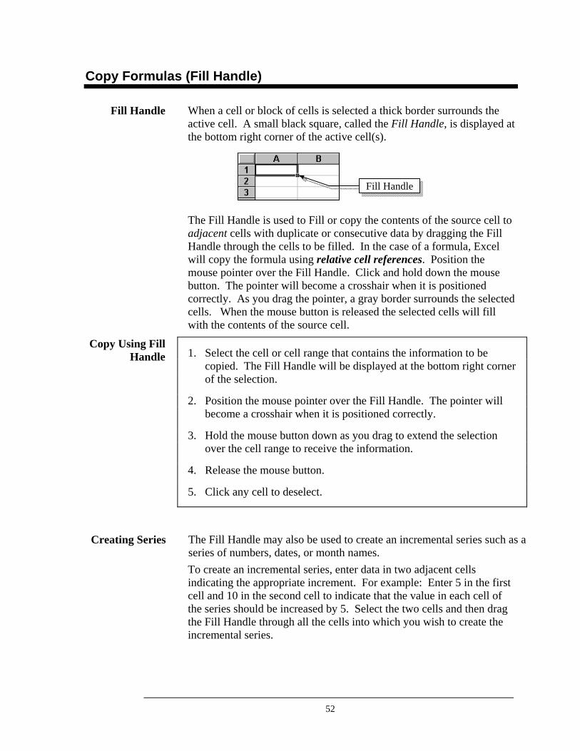
Copy Formulas (Fill Handle)

When a cell or block of cells is selected a thick border surrounds the active cell. A small black square, called the Fill Handle, is displayed at the bottom right corner of the active cell(s).

The Fill Handle is used to Fill or copy the contents of the source cell to adjacent cells with duplicate or consecutive data by dragging the Fill Handle through the cells to be filled. In the case of a formula, Excel will copy the formula using relative cell references. Position the mouse pointer over the Fill Handle. Click and hold down the mouse button. The pointer will become a crosshair when it is positioned correctly. As you drag the pointer, a gray border surrounds the selected cells. When the mouse button is released the selected cells will fill with the contents of the source cell.

1. Select the cell or cell range that contains the information to be copied. The Fill Handle will be displayed at the bottom right corner of the selection.

2. Position the mouse pointer over the Fill Handle. The pointer will become a crosshair when it is positioned correctly.

3. Hold the mouse button down as you drag to extend the selection over the cell range to receive the information.

4. Release the mouse button.

5. Click any cell to deselect.

The Fill Handle may also be used to create an incremental series such as a series of numbers, dates, or month names. To create an incremental series, enter data in two adjacent cells indicating the appropriate increment. For example: Enter 5 in the first cell and 10 in the second cell to indicate that the value in each cell of the series should be increased by 5. Select the two cells and then drag the Fill Handle through all the cells into which you wish to create the incremental series.

Fill Handle

Copy Using Fill Handle

Creating Series

Fill Handle

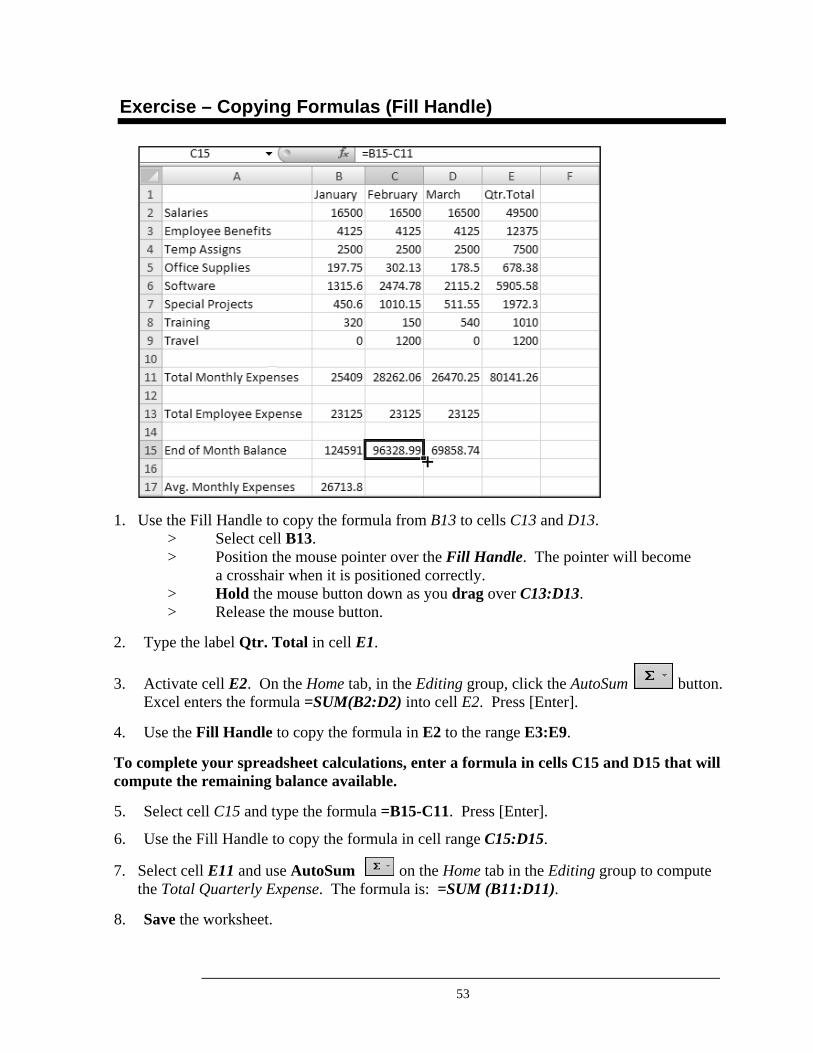
53

Exercise – Copying Formulas (Fill Handle)

1. Use the Fill Handle to copy the formula from B13 to cells C13 and D13. > Select cell B13. > Position the mouse pointer over the Fill Handle. The pointer will become a crosshair when it is positioned correctly. > Hold the mouse button down as you drag over C13:D13. > Release the mouse button.

2. Type the label Qtr. Total in cell E1.

3. Activate cell E2. On the Home tab, in the Editing group, click the AutoSum button. Excel enters the formula =SUM(B2:D2) into cell E2. Press [Enter].

4. Use the Fill Handle to copy the formula in E2 to the range E3:E9.

To complete your spreadsheet calculations, enter a formula in cells C15 and D15 that will compute the remaining balance available.

5. Select cell C15 and type the formula =B15-C11. Press [Enter].

6. Use the Fill Handle to copy the formula in cell range C15:D15.

7. Select cell E11 and use AutoSum on the Home tab in the Editing group to compute the Total Quarterly Expense. The formula is: =SUM (B11:D11).


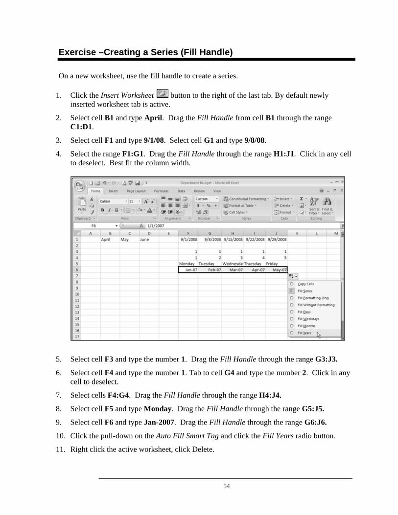
54

Exercise –Creating a Series (Fill Handle)

On a new worksheet, use the fill handle to create a series.

1. Click the Insert Worksheet button to the right of the last tab. By default newly inserted worksheet tab is active.

2. Select cell B1 and type April. Drag the Fill Handle from cell B1 through the range C1:D1.

3. Select cell F1 and type 9/1/08. Select cell G1 and type 9/8/08.

4. Select the range F1:G1. Drag the Fill Handle through the range H1:J1. Click in any cell to deselect. Best fit the column width.

5. Select cell F3 and type the number 1. Drag the Fill Handle through the range G3:J3.

6. Select cell F4 and type the number 1. Tab to cell G4 and type the number 2. Click in any cell to deselect.

7. Select cells F4:G4. Drag the Fill Handle through the range H4:J4.

8. Select cell F5 and type Monday. Drag the Fill Handle through the range G5:J5.

9. Select cell F6 and type Jan-2007. Drag the Fill Handle through the range G6:J6.

10. Click the pull-down on the Auto Fill Smart Tag and click the Fill Years radio button.

11. Right click the active worksheet, click Delete.

55

Notes

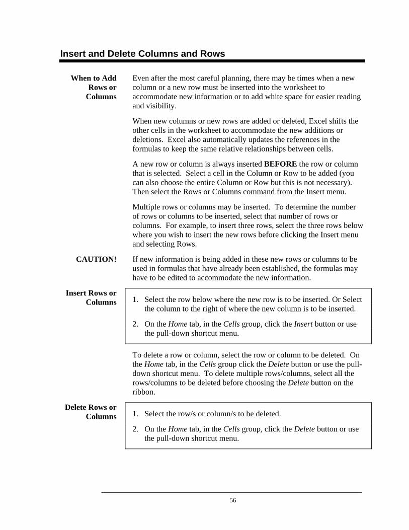
56

Insert and Delete Columns and Rows

Even after the most careful planning, there may be times when a new column or a new row must be inserted into the worksheet to accommodate new information or to add white space for easier reading and visibility.

When new columns or new rows are added or deleted, Excel shifts the other cells in the worksheet to accommodate the new additions or deletions. Excel also automatically updates the references in the formulas to keep the same relative relationships between cells.

A new row or column is always inserted BEFORE the row or column that is selected. Select a cell in the Column or Row to be added (you can also choose the entire Column or Row but this is not necessary). Then select the Rows or Columns command from the Insert menu.

Multiple rows or columns may be inserted. To determine the number of rows or columns to be inserted, select that number of rows or columns. For example, to insert three rows, select the three rows below where you wish to insert the new rows before clicking the Insert menu and selecting Rows.

If new information is being added in these new rows or columns to be used in formulas that have already been established, the formulas may have to be edited to accommodate the new information.

1. Select the row below where the new row is to be inserted. Or Select the column to the right of where the new column is to be inserted.

2. On the Home tab, in the Cells group, click the Insert button or use the pull-down shortcut menu.

To delete a row or column, select the row or column to be deleted. On the Home tab, in the Cells group click the Delete button or use the pull-down shortcut menu. To delete multiple rows/columns, select all the rows/columns to be deleted before choosing the Delete button on the ribbon.

1. Select the row/s or column/s to be deleted.

2. On the Home tab, in the Cells group, click the Delete button or use the pull-down shortcut menu.

When to Add Rows or

Columns

CAUTION!

Insert Rows or Columns

Delete Rows or Columns

57

Exercise - Inserting Rows

1. To insert a row between rows 1 and 2, click row 2. On the Home tab, in the Cells group,

click the Insert button.

2. Click cell A2. Type Employee Expenses: and press Enter.

3. To insert a row between rows 5 and 6, click row 6. On the Home tab, in the Cells group, click the Insert button.

4. Click cell A6. Type Miscellaneous Expenses: and press Enter. Best Fit the column if necessary.

5. Insert two rows above Row 1. These rows will be used next to add a title to this worksheet.

6. Click cells in the row 15 that contain formulas to observe that the formulas have changed to accommodate the new rows.


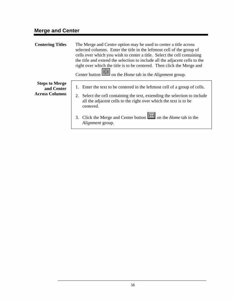
58

Merge and Center

The Merge and Center option may be used to center a title across selected columns. Enter the title in the leftmost cell of the group of cells over which you wish to center a title. Select the cell containing the title and extend the selection to include all the adjacent cells to the right over which the title is to be centered. Then click the Merge and

Center button on the Home tab in the Alignment group.

1. Enter the text to be centered in the leftmost cell of a group of cells.

2. Select the cell containing the text, extending the selection to include all the adjacent cells to the right over which the text is to be centered.

3. Click the Merge and Center button on the Home tab in the Alignment group.

Centering Titles

Steps to Merge and Center

Across Columns

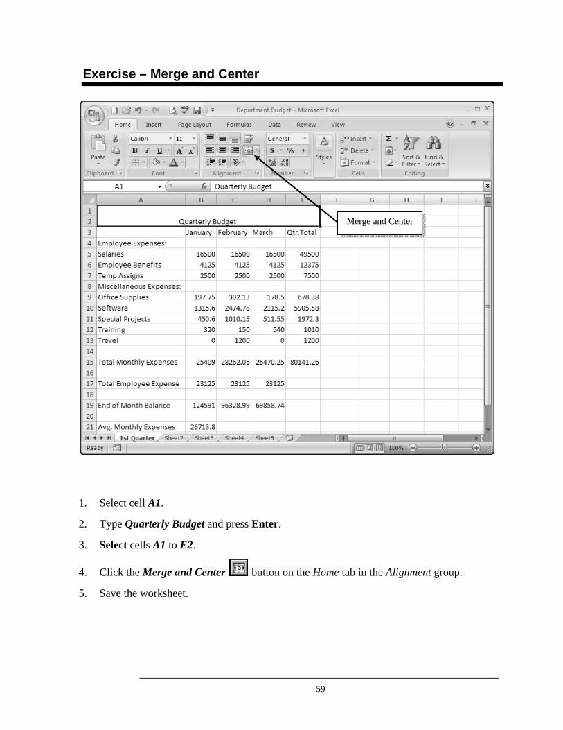
59

Exercise – Merge and Center

1. Select cell A1.

2. Type Quarterly Budget and press Enter.

3. Select cells A1 to E2.

4. Click the Merge and Center button on the Home tab in the Alignment group.


Merge and Center

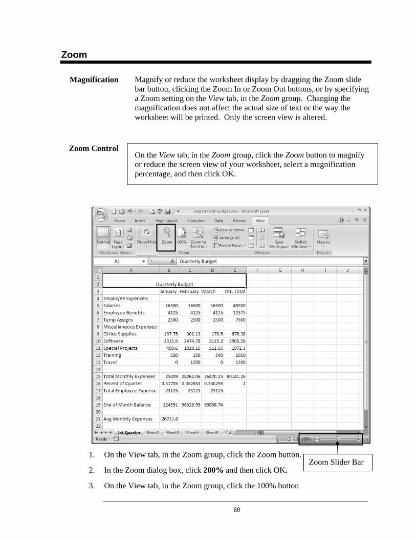
60

Zoom

Magnify or reduce the worksheet display by dragging the Zoom slide bar button, clicking the Zoom In or Zoom Out buttons, or by specifying a Zoom setting on the View tab, in the Zoom group. Changing the magnification does not affect the actual size of text or the way the worksheet will be printed. Only the screen view is altered.

On the View tab, in the Zoom group, click the Zoom button to magnify or reduce the screen view of your worksheet, select a magnification percentage, and then click OK.

1. On the View tab, in the Zoom group, click the Zoom button.

2. In the Zoom dialog box, click 200% and then click OK.

3. On the View tab, in the Zoom group, click the 100% button

Magnification

Zoom Control

Zoom Slider Bar

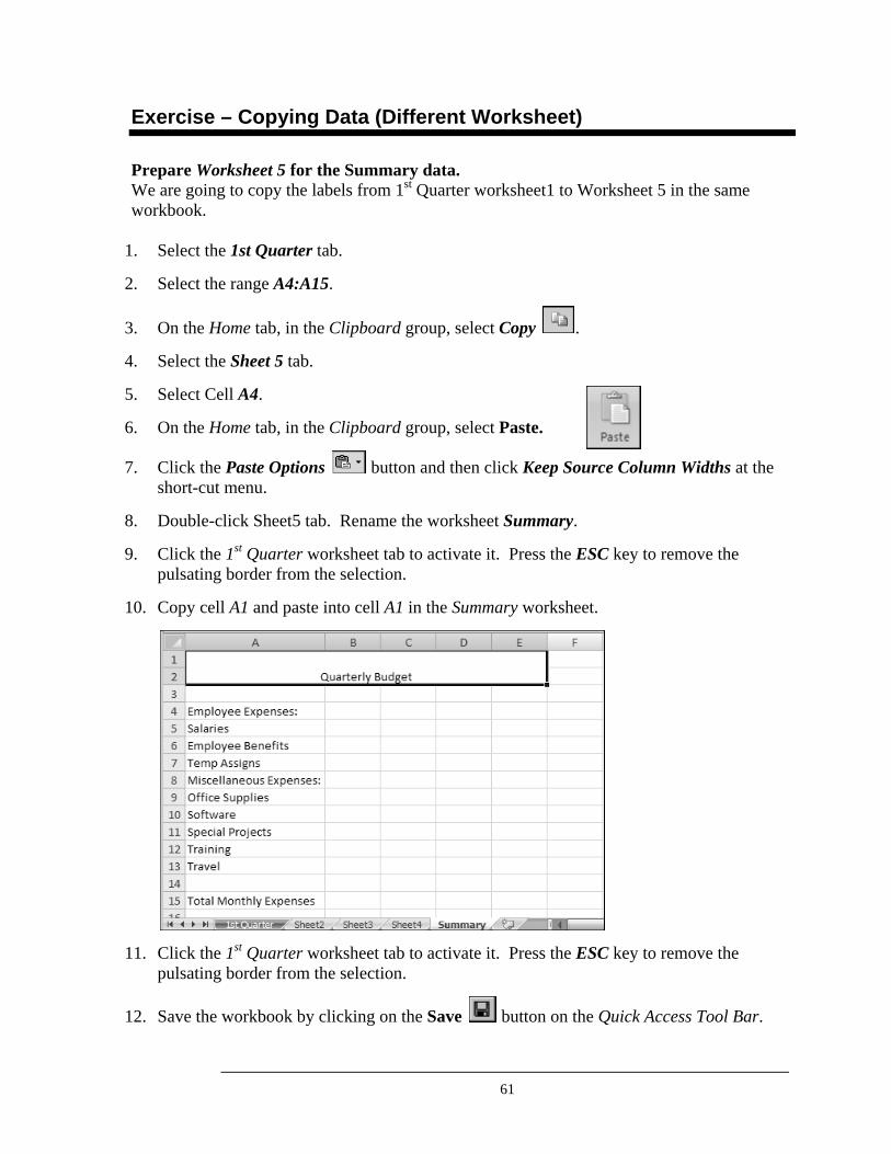
61

Exercise – Copying Data (Different Worksheet)

Prepare Worksheet 5 for the Summary data. We are going to copy the labels from 1st Quarter worksheet1 to Worksheet 5 in the same workbook.

1. Select the 1st Quarter tab.

2. Select the range A4:A15.

3. On the Home tab, in the Clipboard group, select Copy .

4. Select the Sheet 5 tab.

5. Select Cell A4.

6. On the Home tab, in the Clipboard group, select Paste.

7. Click the Paste Options button and then click Keep Source Column Widths at the short-cut menu.

8. Double-click Sheet5 tab. Rename the worksheet Summary.

9. Click the 1st Quarter worksheet tab to activate it. Press the ESC key to remove the pulsating border from the selection.

10. Copy cell A1 and paste into cell A1 in the Summary worksheet.

11. Click the 1st Quarter worksheet tab to activate it. Press the ESC key to remove the pulsating border from the selection.

12. Save the workbook by clicking on the Save button on the Quick Access Tool Bar.

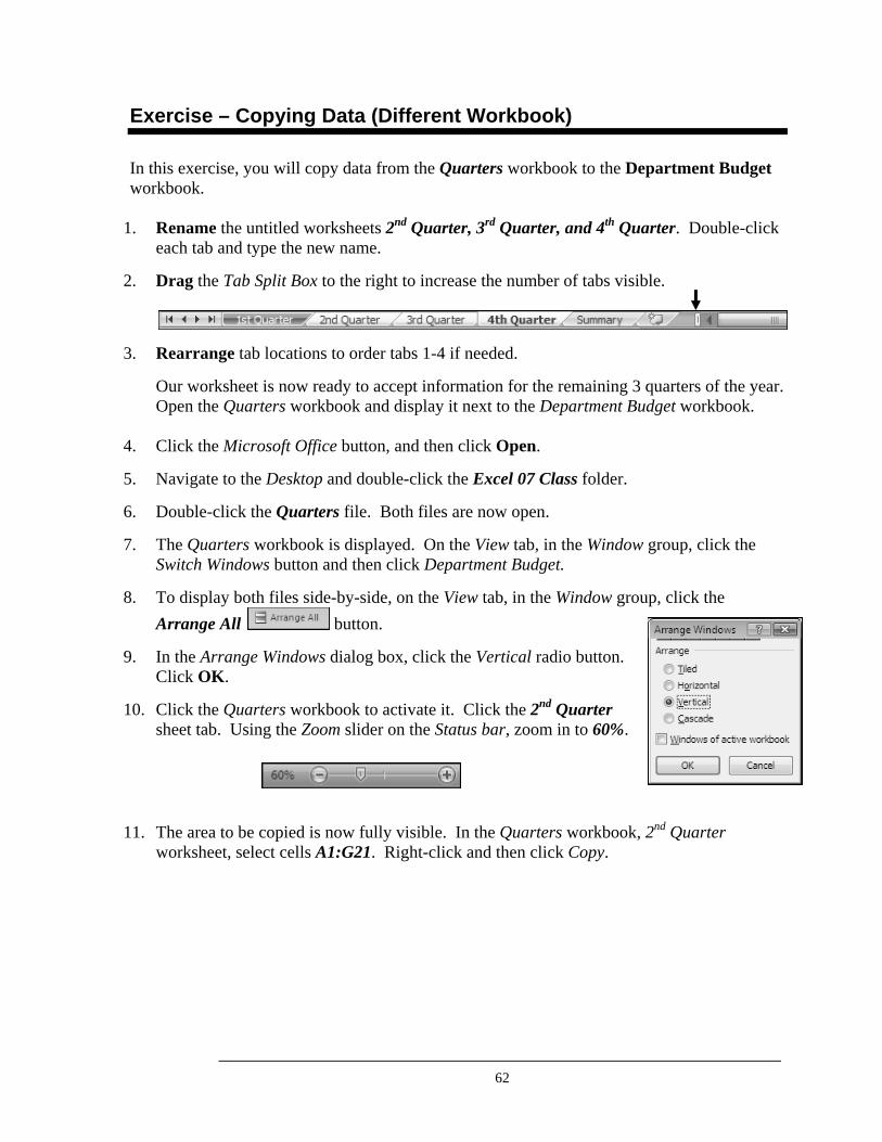
62

Exercise – Copying Data (Different Workbook)

In this exercise, you will copy data from the Quarters workbook to the Department Budget workbook.

1. Rename the untitled worksheets 2nd Quarter, 3rd Quarter, and 4th Quarter. Double-click each tab and type the new name.

2. Drag the Tab Split Box to the right to increase the number of tabs visible.

3. Rearrange tab locations to order tabs 1-4 if needed.

Our worksheet is now ready to accept information for the remaining 3 quarters of the year. Open the Quarters workbook and display it next to the Department Budget workbook.

4. Click the Microsoft Office button, and then click Open.

5. Navigate to the Desktop and double-click the Excel 07 Class folder.

6. Double-click the Quarters file. Both files are now open.

7. The Quarters workbook is displayed. On the View tab, in the Window group, click the Switch Windows button and then click Department Budget.

8. To display both files side-by-side, on the View tab, in the Window group, click the Arrange All button.

9. In the Arrange Windows dialog box, click the Vertical radio button. Click OK.

10. Click the Quarters workbook to activate it. Click the 2nd Quarter sheet tab. Using the Zoom slider on the Status bar, zoom in to 60%.

11. The area to be copied is now fully visible. In the Quarters workbook, 2nd Quarter worksheet, select cells A1:G21. Right-click and then click Copy.

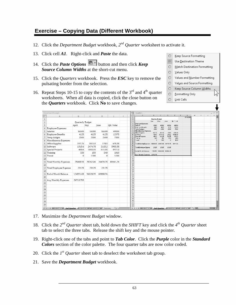
63

Exercise – Copying Data (Different Workbook)

12. Click the Department Budget workbook, 2nd Quarter worksheet to activate it.

13. Click cell A1. Right-click and Paste the data.

14. Click the Paste Options button and then click Keep Source Column Widths at the short-cut menu.

15. Click the Quarters workbook. Press the ESC key to remove the pulsating border from the selection.

16. Repeat Steps 10-15 to copy the contents of the 3rd and 4th quarter worksheets. When all data is copied, click the close button on the Quarters workbook. Click No to save changes.

17. Maximize the Department Budget window.

18. Click the 2nd Quarter sheet tab, hold down the SHIFT key and click the 4th Quarter sheet tab to select the three tabs. Release the shift key and the mouse pointer.

19. Right-click one of the tabs and point to Tab Color. Click the Purple color in the Standard Colors section of the color palette. The four quarter tabs are now color coded.

20. Click the 1st Quarter sheet tab to deselect the worksheet tab group.

21. Save the Department Budget workbook.

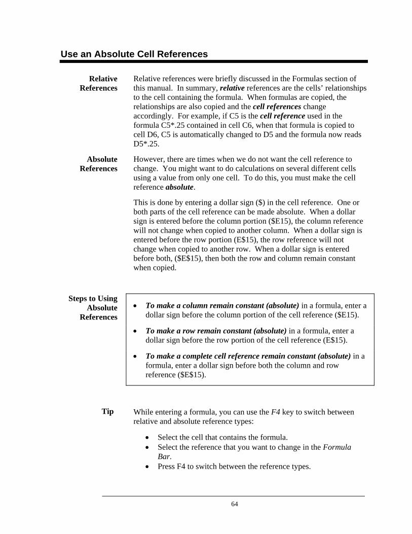
64

Use an Absolute Cell References

Relative references were briefly discussed in the Formulas section of this manual. In summary, relative references are the cells’ relationships to the cell containing the formula. When formulas are copied, the relationships are also copied and the cell references change accordingly. For example, if C5 is the cell reference used in the formula C5*.25 contained in cell C6, when that formula is copied to cell D6, C5 is automatically changed to D5 and the formula now reads D5*.25.

However, there are times when we do not want the cell reference to change. You might want to do calculations on several different cells using a value from only one cell. To do this, you must make the cell reference absolute.

This is done by entering a dollar sign ($) in the cell reference. One or both parts of the cell reference can be made absolute. When a dollar sign is entered before the column portion ($E15), the column reference will not change when copied to another column. When a dollar sign is entered before the row portion (E$15), the row reference will not change when copied to another row. When a dollar sign is entered before both, ($E$15), then both the row and column remain constant when copied.

• To make a column remain constant (absolute) in a formula, enter a dollar sign before the column portion of the cell reference ($E15).

• To make a row remain constant (absolute) in a formula, enter a dollar sign before the row portion of the cell reference (E$15).

• To make a complete cell reference remain constant (absolute) in a formula, enter a dollar sign before both the column and row reference ($E$15).

While entering a formula, you can use the F4 key to switch between relative and absolute reference types:

• Select the cell that contains the formula. • Select the reference that you want to change in the Formula

Bar. • Press F4 to switch between the reference types.

Relative References

Absolute References

Steps to Using Absolute

References

Tip

65

Exercise – Using an Absolute Cell References

Calculate the percentage of each month’s total expense of the Total Quarterly Expense. Divide the Total Quarter Expense (E15) into each month’s total. You need to have cell E15 remain constant (absolute) in all of the monthly percentage formulas.

1. Select cell A16 and enter the label Percent of Quarter.

2. Tab to cell B16 and enter the appropriate formula: =B15/$E$15. Press Enter. Remember that Total Quarterly Expense must remain absolute when the formula is copied to C16 and D16, thus use the $ sign in the cell reference. Notice the result does not look like a percentage. You will format it later.

3. Select cell B16.

4. Use the Fill Handle to auto fill cells C16:D16. Notice the Total Quarterly Expense reference (E15) stayed the same for all three months. There was no cell reference change.

5. Save the workbook.

66

Use a 3-D Cell Reference

There may be times when you will need to summarize data from different worksheets. For example, if you want to calculate the annual grand total for the Salaries expenditures, you will need to create a separate worksheet with a formula that includes a 3-D reference.

A 3-D reference refers to the same cell or range on multiple sheets. In this case the cell that contains the quarterly total for each budget category on all four worksheets will be used in the 3-D reference.

The Summary worksheet will display the result in the cell and the formula with 3-D reference will display in the formula bar.

When a cell reference from another worksheets is used in a formula, you must include the sheet reference (sheet name) with the cell reference. An exclamation point is used to separate the sheet reference from the cell reference. For example, you would refer to Cell B5 on Sheet1 as:

Sheet1! B5

If the sheet name contains spaces, single quotation marks must enclose the sheet name in the formula. For example: '1st Qtr Budget'!B5 refers to cell B5 on the worksheet named 1st Qtr Budget.

1. Find the sheet name and cell number that you want to be rolled over to another sheet. Remember the sheet and cell number or write it down.

2. Go to the sheet that will contain the new reference.

3. Select the cell that you want the cell reference to be in.

4. Type your formula and add your correct sheet name, exclamation point and your cell reference.

3-D Reference

Reference Naming

Convention

Steps to Use Cell References

Exclamation Point separates Sheet Name from Cell Reference

Sheet Name Cell Reference

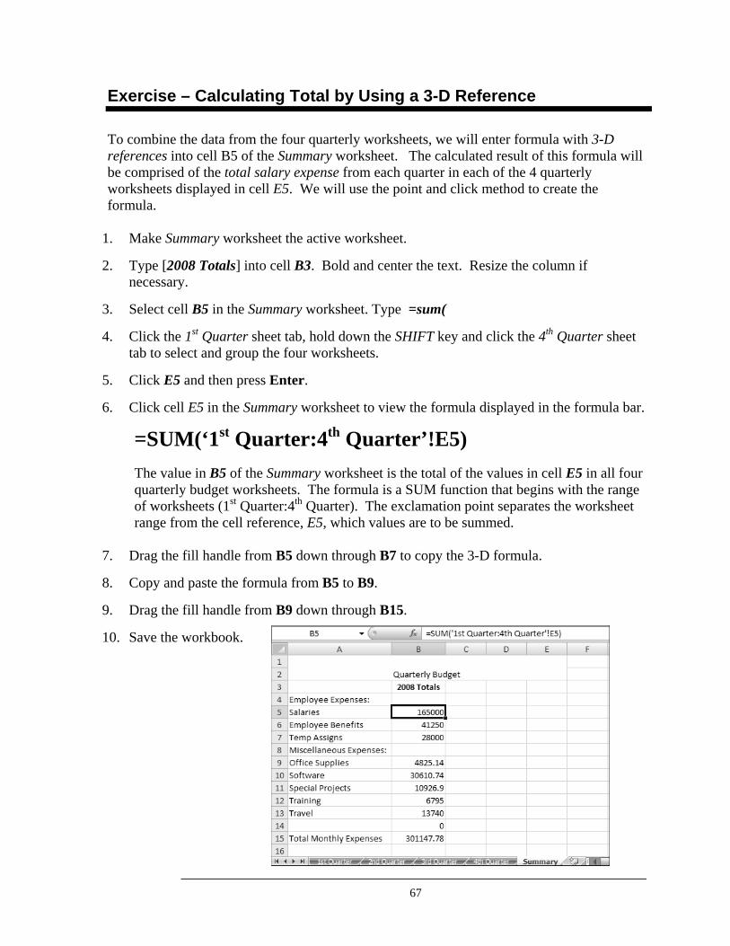
67

Exercise – Calculating Total by Using a 3-D Reference

To combine the data from the four quarterly worksheets, we will enter formula with 3-D references into cell B5 of the Summary worksheet. The calculated result of this formula will be comprised of the total salary expense from each quarter in each of the 4 quarterly worksheets displayed in cell E5. We will use the point and click method to create the formula.

1. Make Summary worksheet the active worksheet.

2. Type [2008 Totals] into cell B3. Bold and center the text. Resize the column if necessary.

3. Select cell B5 in the Summary worksheet. Type =sum(

4. Click the 1st Quarter sheet tab, hold down the SHIFT key and click the 4th Quarter sheet tab to select and group the four worksheets.

5. Click E5 and then press Enter.

6. Click cell E5 in the Summary worksheet to view the formula displayed in the formula bar.

=SUM(‘1st Quarter:4th Quarter’!E5) The value in B5 of the Summary worksheet is the total of the values in cell E5 in all four quarterly budget worksheets. The formula is a SUM function that begins with the range of worksheets (1st Quarter:4th Quarter). The exclamation point separates the worksheet range from the cell reference, E5, which values are to be summed.

7. Drag the fill handle from B5 down through B7 to copy the 3-D formula.

8. Copy and paste the formula from B5 to B9.

9. Drag the fill handle from B9 down through B15.


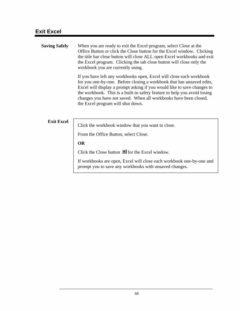
68

Exit Excel

When you are ready to exit the Excel program, select Close at the Office Button or click the Close button for the Excel window. Clicking the title bar close button will close ALL open Excel workbooks and exit the Excel program. Clicking the tab close button will close only the workbook you are currently using.

If you have left any workbooks open, Excel will close each workbook for you one-by-one. Before closing a workbook that has unsaved edits, Excel will display a prompt asking if you would like to save changes to the workbook. This is a built-in safety feature to help you avoid losing changes you have not saved. When all workbooks have been closed, the Excel program will shut down.

Click the workbook window that you want to close.

From the Office Button, select Close.

OR

Click the Close button for the Excel window.

If workbooks are open, Excel will close each workbook one-by-one and prompt you to save any workbooks with unsaved changes.

Saving Safely

Exit Excel

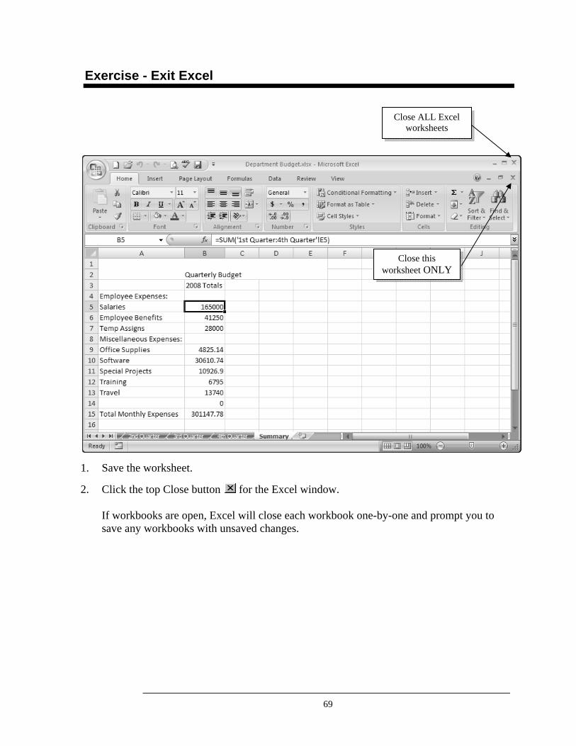
69

Exercise - Exit Excel


2. Click the top Close button for the Excel window. If workbooks are open, Excel will close each workbook one-by-one and prompt you to save any workbooks with unsaved changes.

Close ALL Excel worksheets

Close this worksheet ONLY

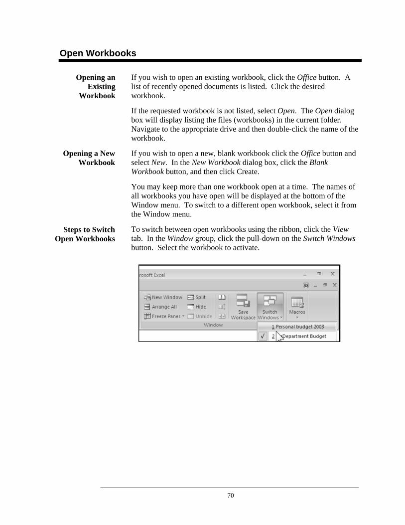
70

Open Workbooks

If you wish to open an existing workbook, click the Office button. A list of recently opened documents is listed. Click the desired workbook.

If the requested workbook is not listed, select Open. The Open dialog box will display listing the files (workbooks) in the current folder. Navigate to the appropriate drive and then double-click the name of the workbook.

If you wish to open a new, blank workbook click the Office button and select New. In the New Workbook dialog box, click the Blank Workbook button, and then click Create.

You may keep more than one workbook open at a time. The names of all workbooks you have open will be displayed at the bottom of the Window menu. To switch to a different open workbook, select it from the Window menu.

To switch between open workbooks using the ribbon, click the View tab. In the Window group, click the pull-down on the Switch Windows button. Select the workbook to activate.

Opening an Existing

Workbook

Opening a New Workbook

Steps to Switch Open Workbooks

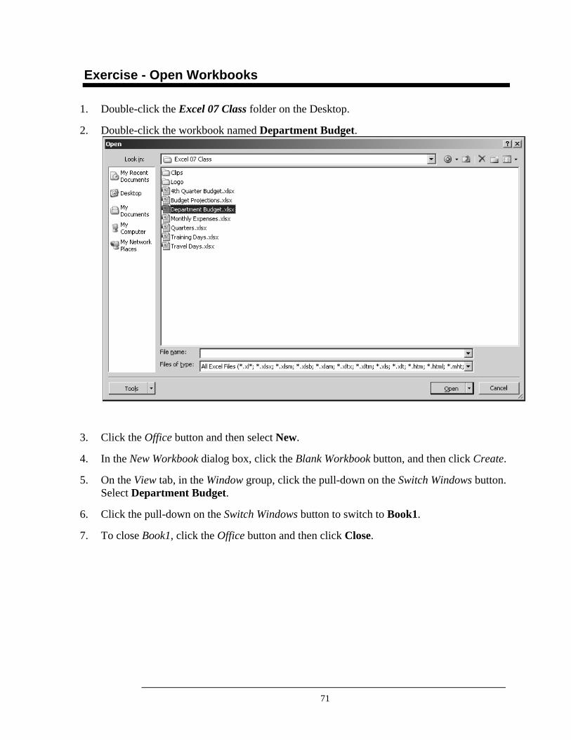
71

Exercise - Open Workbooks

1. Double-click the Excel 07 Class folder on the Desktop.

2. Double-click the workbook named Department Budget.

3. Click the Office button and then select New.

4. In the New Workbook dialog box, click the Blank Workbook button, and then click Create.

5. On the View tab, in the Window group, click the pull-down on the Switch Windows button. Select Department Budget.

6. Click the pull-down on the Switch Windows button to switch to Book1.

7. To close Book1, click the Office button and then click Close.

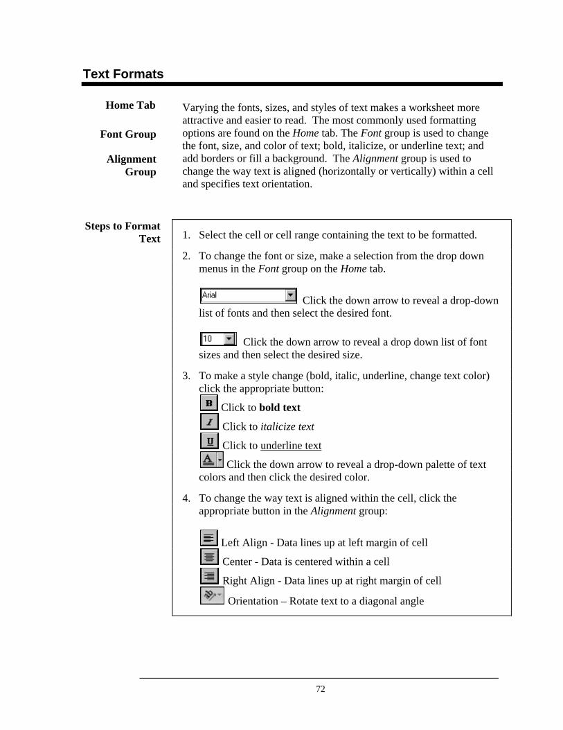
72

Text Formats

Varying the fonts, sizes, and styles of text makes a worksheet more attractive and easier to read. The most commonly used formatting options are found on the Home tab. The Font group is used to change the font, size, and color of text; bold, italicize, or underline text; and add borders or fill a background. The Alignment group is used to change the way text is aligned (horizontally or vertically) within a cell and specifies text orientation.

1. Select the cell or cell range containing the text to be formatted.

2. To change the font or size, make a selection from the drop down menus in the Font group on the Home tab.

Click the down arrow to reveal a drop-down list of fonts and then select the desired font.

Click the down arrow to reveal a drop down list of font sizes and then select the desired size.

3. To make a style change (bold, italic, underline, change text color) click the appropriate button:

Click to bold text

Click to italicize text

Click to underline text

Click the down arrow to reveal a drop-down palette of text colors and then click the desired color.

4. To change the way text is aligned within the cell, click the appropriate button in the Alignment group:

Left Align - Data lines up at left margin of cell

Center - Data is centered within a cell

Right Align - Data lines up at right margin of cell

Orientation – Rotate text to a diagonal angle

Font Group

Home Tab

Alignment Group

Steps to Format Text

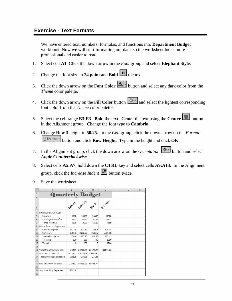
73

Exercise - Text Formats

We have entered text, numbers, formulas, and functions into Department Budget workbook. Now we will start formatting our data, so the worksheet looks more professional and easier to read.

1. Select cell A1. Click the down arrow in the Font group and select Elephant Style.

2. Change the font size to 24 point and Bold the text.

3. Click the down arrow on the Font Color button and select any dark color from the Theme color palette.

4. Click the down arrow on the Fill Color button and select the lightest corresponding font color from the Theme color palette.

5. Select the cell range B3:E3. Bold the text. Center the text using the Center button in the Alignment group. Change the font type to Cambria.

6. Change Row 3 height to 50.25. In the Cell group, click the down arrow on the Format

button and click Row Height. Type in the height and click OK.

7. In the Alignment group, click the down arrow on the Orientation button and select Angle Counterclockwise.

8. Select cells A5:A7, hold down the CTRL key and select cells A9:A13. In the Alignment

group, click the Increase Indent button twice.


74

Number Formats

If you look at your worksheet as it is displayed on the screen, you will see that your dollar amounts are not formatted properly. When you first enter numbers, they appear in the General format. They are simply numbers displayed as precisely as possible. Using buttons on the Home tab, in the Number group numbers can be formatted to include dollar signs, percent signs, and comma separators as needed, and you can also specify the number of decimal places to be displayed.

To change number formats, first select the cells containing the numbers that are to be affected. Next, click the appropriate button on the ribbon.

Adds a dollar sign $ at the beginning of the number, adds a comma in front of every third number from the left of the decimal point, and displays two decimal places. Example: $17,454.15.

Multiplies the number by 100 and adds a percent % sign at the end. Example: If .20 is entered it is displayed as 20%

Adds a comma in front of every third number from the left of the decimal point, and displays two decimal places. Example: 17,454.15

Adds the display of one decimal place each time this button is clicked.

Eliminates the display of one decimal place each time this button is clicked.

1. Select the cell or cell range that contains the number(s) to be formatted.

2. Click the appropriate button on the Formatting toolbar.

Sometimes changing the number format will cause the cell entries to become too wide to fit in the cells. For example, if you change from general to currency format, a $ sign, commas, and decimal places are added. If a numerical cell entry is too wide to fit, Excel will indicate that by displaying ####### in the cell. To redisplay the proper cell entries, increase the column width.

Formatting Numbers

Currency

Percent

Comma

Increase Decimal

Decrease Decimal

Apply Number Formats

Tip

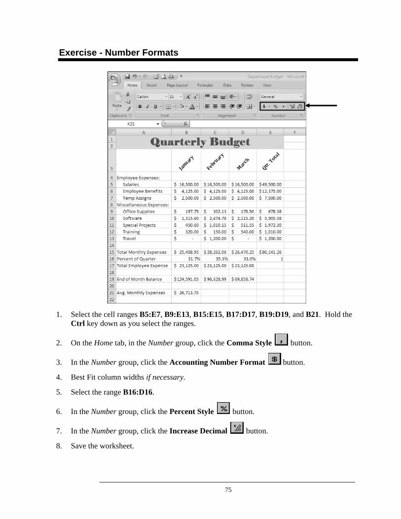
75

Exercise - Number Formats

1. Select the cell ranges B5:E7, B9:E13, B15:E15, B17:D17, B19:D19, and B21. Hold the Ctrl key down as you select the ranges.

2. On the Home tab, in the Number group, click the Comma Style button.

3. In the Number group, click the Accounting Number Format button.

4. Best Fit column widths if necessary.

5. Select the range B16:D16.

6. In the Number group, click the Percent Style button.

7. In the Number group, click the Increase Decimal button.


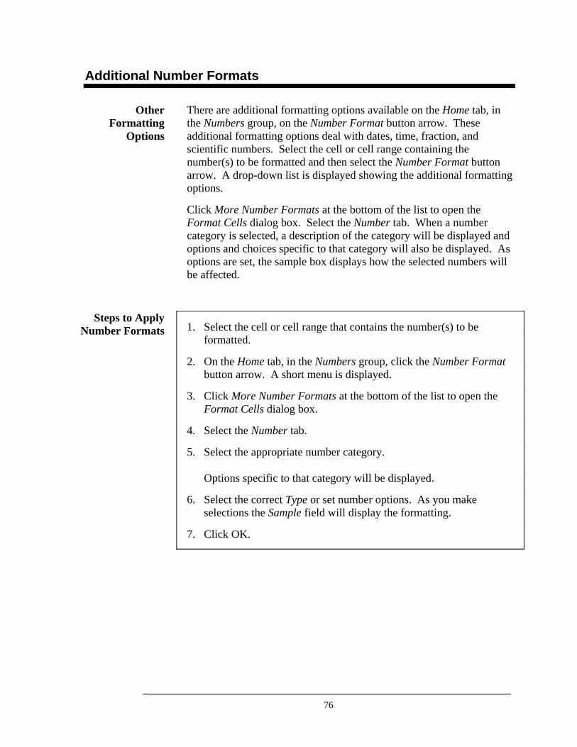
76

Additional Number Formats

There are additional formatting options available on the Home tab, in the Numbers group, on the Number Format button arrow. These additional formatting options deal with dates, time, fraction, and scientific numbers. Select the cell or cell range containing the number(s) to be formatted and then select the Number Format button arrow. A drop-down list is displayed showing the additional formatting options.

Click More Number Formats at the bottom of the list to open the Format Cells dialog box. Select the Number tab. When a number category is selected, a description of the category will be displayed and options and choices specific to that category will also be displayed. As options are set, the sample box displays how the selected numbers will be affected.

1. Select the cell or cell range that contains the number(s) to be formatted.

2. On the Home tab, in the Numbers group, click the Number Format button arrow. A short menu is displayed.

3. Click More Number Formats at the bottom of the list to open the Format Cells dialog box.

4. Select the Number tab.

5. Select the appropriate number category. Options specific to that category will be displayed.

6. Select the correct Type or set number options. As you make selections the Sample field will display the formatting.

7. Click OK.

Other Formatting

Options

Steps to Apply Number Formats

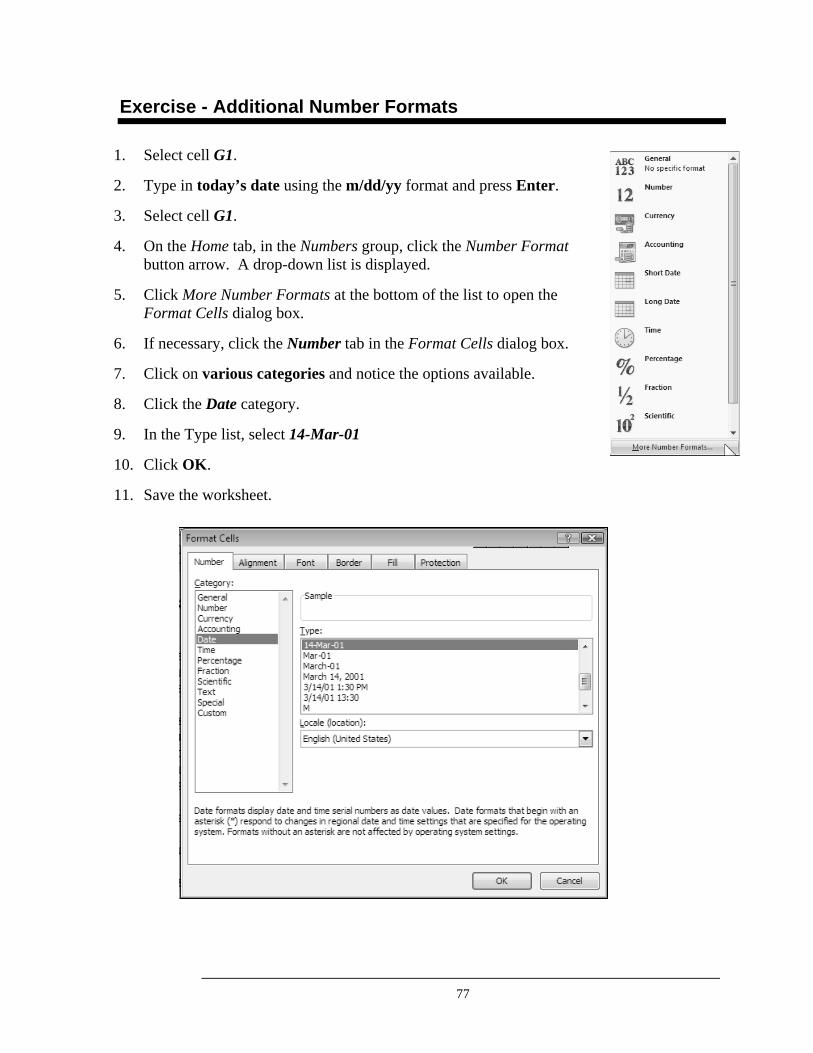
77

Exercise - Additional Number Formats

1. Select cell G1.

2. Type in today’s date using the m/dd/yy format and press Enter.

3. Select cell G1.

4. On the Home tab, in the Numbers group, click the Number Format button arrow. A drop-down list is displayed.

5. Click More Number Formats at the bottom of the list to open the Format Cells dialog box.

6. If necessary, click the Number tab in the Format Cells dialog box.

7. Click on various categories and notice the options available.

8. Click the Date category.

9. In the Type list, select 14-Mar-01

10. Click OK.


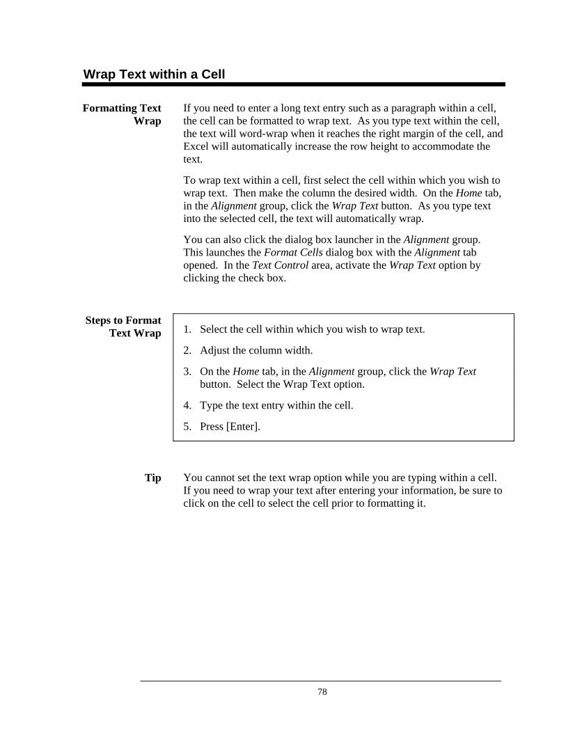
78

Wrap Text within a Cell

If you need to enter a long text entry such as a paragraph within a cell, the cell can be formatted to wrap text. As you type text within the cell, the text will word-wrap when it reaches the right margin of the cell, and Excel will automatically increase the row height to accommodate the text.

To wrap text within a cell, first select the cell within which you wish to wrap text. Then make the column the desired width. On the Home tab, in the Alignment group, click the Wrap Text button. As you type text into the selected cell, the text will automatically wrap.

You can also click the dialog box launcher in the Alignment group. This launches the Format Cells dialog box with the Alignment tab opened. In the Text Control area, activate the Wrap Text option by clicking the check box.

1. Select the cell within which you wish to wrap text.

2. Adjust the column width.

3. On the Home tab, in the Alignment group, click the Wrap Text button. Select the Wrap Text option.

4. Type the text entry within the cell.

5. Press [Enter].

You cannot set the text wrap option while you are typing within a cell. If you need to wrap your text after entering your information, be sure to click on the cell to select the cell prior to formatting it.

Formatting Text Wrap

Steps to Format Text Wrap

Tip

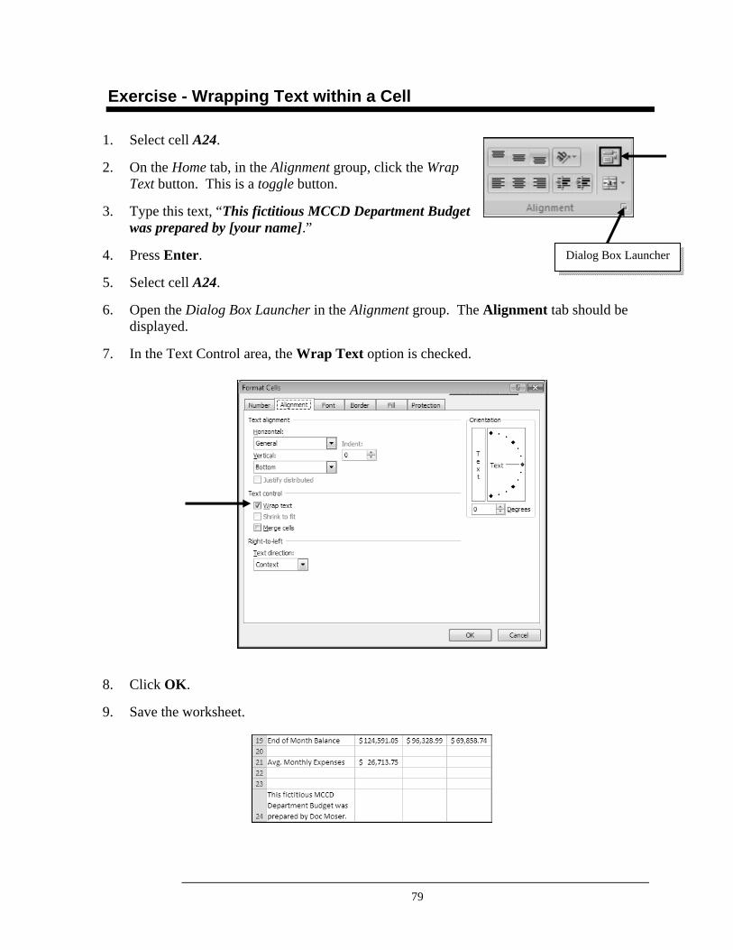
79

Exercise - Wrapping Text within a Cell

1. Select cell A24.

2. On the Home tab, in the Alignment group, click the Wrap Text button. This is a toggle button.

3. Type this text, “This fictitious MCCD Department Budget was prepared by [your name].”

4. Press Enter.

5. Select cell A24.

6. Open the Dialog Box Launcher in the Alignment group. The Alignment tab should be displayed.

7. In the Text Control area, the Wrap Text option is checked.

8. Click OK.


Dialog Box Launcher

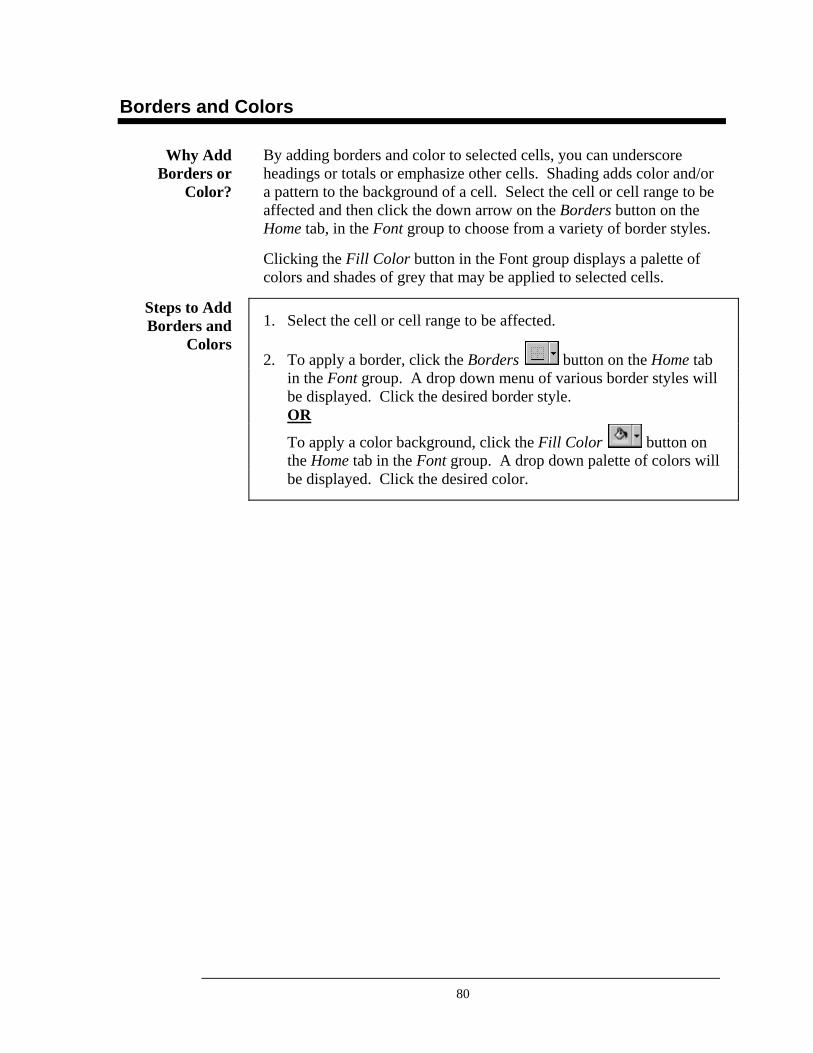
80

Borders and Colors

By adding borders and color to selected cells, you can underscore headings or totals or emphasize other cells. Shading adds color and/or a pattern to the background of a cell. Select the cell or cell range to be affected and then click the down arrow on the Borders button on the Home tab, in the Font group to choose from a variety of border styles.

Clicking the Fill Color button in the Font group displays a palette of colors and shades of grey that may be applied to selected cells.

1. Select the cell or cell range to be affected.

2. To apply a border, click the Borders button on the Home tab in the Font group. A drop down menu of various border styles will be displayed. Click the desired border style. OR

To apply a color background, click the Fill Color button on the Home tab in the Font group. A drop down palette of colors will be displayed. Click the desired color.

Why Add Borders or

Color?

Steps to Add Borders and

Colors

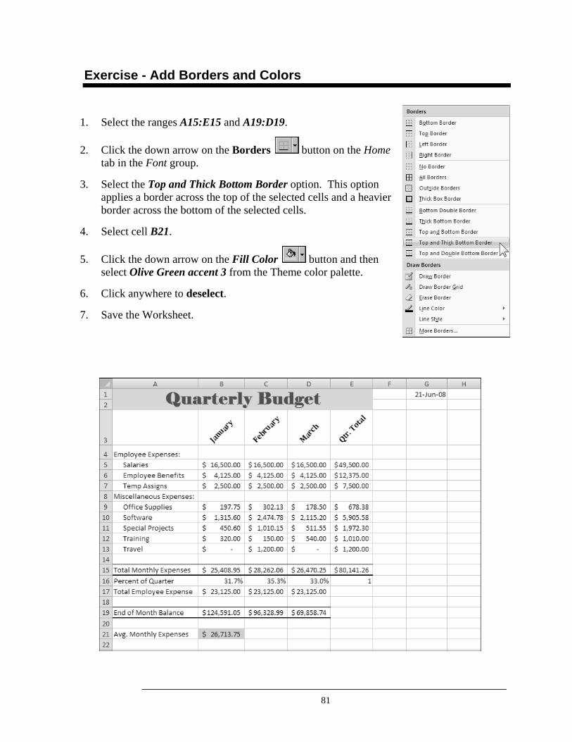
81

Exercise - Add Borders and Colors

1. Select the ranges A15:E15 and A19:D19.

2. Click the down arrow on the Borders button on the Home tab in the Font group.

3. Select the Top and Thick Bottom Border option. This option applies a border across the top of the selected cells and a heavier border across the bottom of the selected cells.

4. Select cell B21.

5. Click the down arrow on the Fill Color button and then select Olive Green accent 3 from the Theme color palette.


7. Save the Worksheet.

82

Cell Styles

Excel 2007 has several built-in cell styles that you can apply, modify, or combine to create your own custom cell style. The cell style is a set of formatting characteristics including fonts, font sizes, number formats, cell borders, and cell shading. You can also specify a cell style that locks cells to prevent others from changing specific cells such as formulas.

Cell styles are based on the workbook theme that is applied to the entire workbook. When you switch to another theme, the cell styles are updated to match the new theme.

To apply a cell style, select the cells you want to format and click any style in the Cell Styles gallery located on the Home tab, in the Styles group at the Cell Styles drop-down menu.

A new feature of Excel 2007 displays a live preview of a format when you move your mouse pointer over it. You can create your own style by clicking the New Cell Style option at the bottom of the gallery. This will display the Style dialog box. Type the name of the new style and check desired formatting options. When you click the Format button, the Format Cells dialog box appears. Click OK when you are finished setting the formatting characteristics of your new style to make the style available in the Cell Styles gallery.

To delete a custom style, open the Cell Styles gallery, right-click the style, and then click Delete.

1. Select the cells you want to format.

2. On the Home tab, in the Styles group, click Cell Styles.

3. Click the cell style you want to apply.

1. On the Home tab, in the Styles group, click Cell Styles.

2. Click New Cell Style.

3. In the Style Name box, type a name for the new style. Clear the check boxes for any formatting that you do not want to include.

4. Click Format. On the various tabs of the Format Cells dialog box, select desired formatting and then click OK.

Customize the Format Style

Based on Themes

Live Previews

Deleting a Style

Steps to Select a Predefined Style

Steps to Create a Custom Style

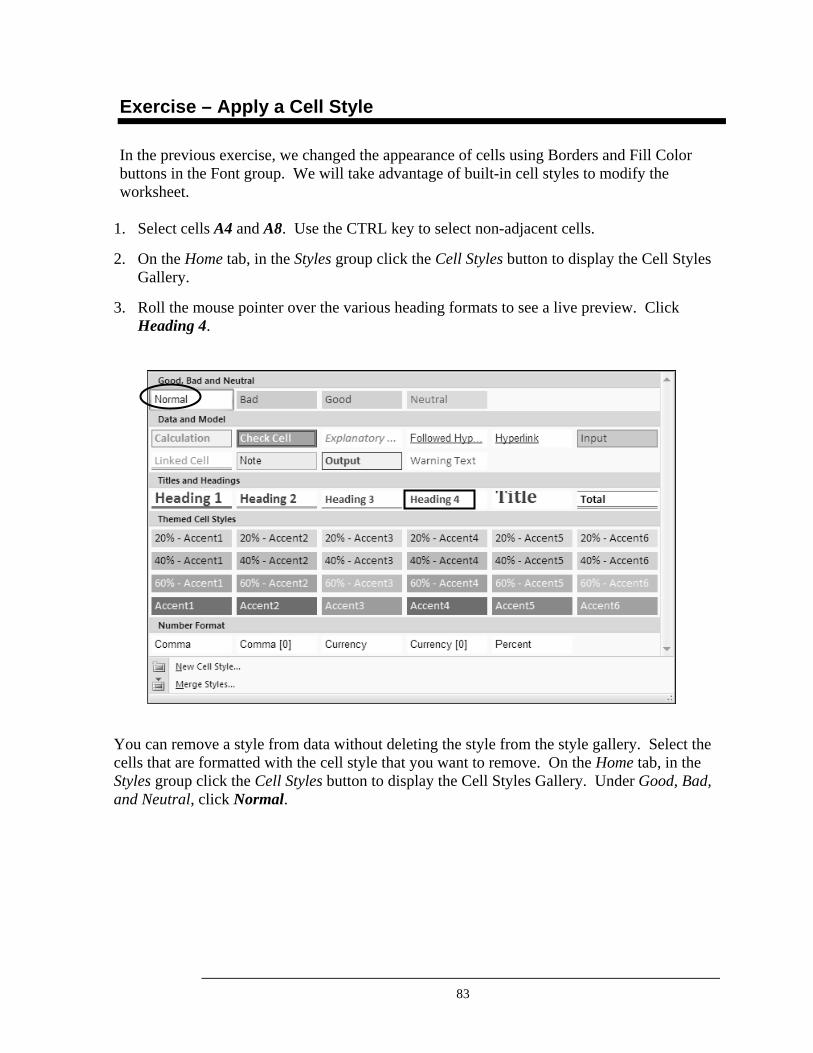
83

Exercise – Apply a Cell Style

In the previous exercise, we changed the appearance of cells using Borders and Fill Color buttons in the Font group. We will take advantage of built-in cell styles to modify the worksheet.

1. Select cells A4 and A8. Use the CTRL key to select non-adjacent cells.

2. On the Home tab, in the Styles group click the Cell Styles button to display the Cell Styles Gallery.

3. Roll the mouse pointer over the various heading formats to see a live preview. Click Heading 4.

You can remove a style from data without deleting the style from the style gallery. Select the cells that are formatted with the cell style that you want to remove. On the Home tab, in the Styles group click the Cell Styles button to display the Cell Styles Gallery. Under Good, Bad, and Neutral, click Normal.

84

Exercise – Create a Custom Cell Style

In this exercise, we will design a new style for the cells containing Total Monthly Expenses data.


2. At the bottom of the gallery window, click New Cell Style. The Style dialog box opens.

3. In the Style Name box, type Expenses. Click the Format button.

4. The Custom Lists dialog box contains several tabs. Click the Number tab. In the Category list, click Currency.

5. Click the Font tab. Change the font to Rockwell, font style is Bold, size is 11pt.

6. Click the Border tab. Click the Outline button.

7. Click the Fill tab. Click the Fill Effects button.

8. Click the radio button for Two colors,

9. Click the radio button for Horizontal shading style.

10. Click the first Variant option.

85

Exercise – Creating a Custom Cell Style

11. Click the pull-down for Color 2. Select the color that complements your title cell. Click the second to last color in the theme group.

12. Color 1 is white. You should not have to change it. If necessary, use the pull-down to change the color to white.

13. Click OK.

14. Click the Protection tab.

15. Click the Locked check box.

16. Click OK to close the Custom Lists dialog box.

17. The Style dialog box displays the modified settings for the Expenses cell style. Click OK.

18. Apply the style to Total Monthly Expenses. Select cells B15:E15.


20. Click the Expenses style.

To delete a predefined or custom cell style, display the cell styles gallery. Right-click the cell style you want to delete and then click Delete. The style is deleted from the gallery and removed from all formatted cells using the style.

86

Themes

Excel provides several predefined workbook themes which may be used to quickly format all worksheets for a professional and modern look. A combination of colors, fonts, and effects are coordinated to give your organization a branded feel. Workbook themes that are applied affect the cell styles that you can use in your worksheet. Themes are shared in Excel, Word, and PowerPoint to create a consistent look for all business publications.

The theme gallery displays the available predefined themes under the Built-In option. By changing the colors, the fonts, or the fill effects you can customize a workbook theme. Changes that you make to one or more of these components immediately affect the styles that you applied in the active workbook. If you save the changes as a customized theme, you can apply these changes to a new workbook.

1. Click the Page Layout tab, Themes group, Themes button.

2. Move the mouse pointer over the themes in the drop-down gallery to see a live preview of the various colors and fonts and then click the theme you want to apply.

1. On the Page Layout tab, in the Themes group, click Colors. At the bottom of the drop-down, click Create New Theme Colors, click the button of the color element that you want to change, and then select the new color. In the Name box, type a name for the new theme colors. Save.

2. Click Fonts. At the bottom of the drop-down, click Create New Theme Fonts. In the Heading and Body Font boxes, select the fonts for the new theme. In the Name box, type a name for the new theme fonts. Save.

3. Click Effects. Click the effect that you want to use.

1. Click the Page Layout tab, Themes group, Themes button.

2. Click Save Current Theme.

3. In the File Name box, type a name for the new theme. Save.

Predefined Styles

Customize the Theme

Steps to Select a Predefined

Theme

Steps to Create a Custom Theme

Steps to Save a New Theme

87

Exercise – Apply a Predefined Theme

1. On the Page Layout tab, in the Themes group, click the Theme button.

2. Move the mouse pointer over each of the themes in the drop-down gallery to see a live preview of the various colors and fonts applied to the worksheet.

3. Click Flow.

4. Select cell B21. On the Home tab, in the Font group, click the Fill Color button.

5. Click No Fill.


88

Comments

Using comments to add notes to a worksheet can help you make a worksheet easier to understand by providing additional information for the data it contains. Comments can be added to data cells or column headings to provide a guide for data entry. When a cell contains a comment, a red indicator appears in the corner of the cell. When you rest the mouse pointer on the cell, the comment appears. Comments can be edited, formatted, and moved, resized, copied, displayed, hidden, printed, and deleted.

1. Select the cell to contain the comment.

2. On the Review tab, in the Comments group, click New Comment.

3. Type the text of the comment in the text box.

4. Click anywhere outside the text box to close it.

Position the mouse pointer over the cell containing the comment. A pop-up window will display the comment.

1. On the Review tab, in the Comments group, click Show All Comments.

2. To hide the comments, click the Show All Comments button again.

1. Click the first cell that contains a comment that you want to review.

2. To review the next comment, on the Review tab, in the Comments group, click Next or Previous to view comments in sequence or reverse order.

1. Click the cell that contains a comment that you want to delete.

2. On the Review tab, in the Comments group, click Delete. OR

3. On the Review tab, in the Comments group, click Show/Hide Comment to display the comment.

4. Click the comment box border and then press the DELETE key.

Excel Notes are now Comments!

Add Comments to a Cell

View Comments

Steps to Display/Hide All

Comments

Review all Comments in a

Workbook

Delete a Comment

89

Exercise – Add Comments

1. Click the 1st Quarter sheet tab.

2. Select cell E9.

3. On the Review tab, in the Comments group, click New Comment.

4. In the Comment box, type, This amount does not include any Copy Center costs incurred in January.

5. Use the size handles to resize the comment box to fit the text.

6. Click cell C13.

7. In the Comments group, click New Comment.

8. In the Comment box, type, This amount includes travel to other colleges.

9. Use the size handles to resize the comment box to fit the text


11. Move your mouse over the red corner indicators to view your Comments.

12. In the Comments group, click Show All Comments. Click Show All Comments.


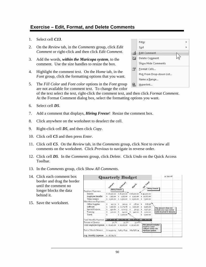
90

Exercise – Edit, Format, and Delete Comments

1. Select cell C13.

2. On the Review tab, in the Comments group, click Edit Comment or right-click and then click Edit Comment.

3. Add the words, within the Maricopa system, to the comment. Use the size handles to resize the box.

4. Highlight the comment text. On the Home tab, in the Font group, click the formatting options that you want.

5. The Fill Color and Font color options in the Font group are not available for comment text. To change the color of the text select the text, right-click the comment text, and then click Format Comment. At the Format Comment dialog box, select the formatting options you want.

6. Select cell D5.

7. Add a comment that displays, Hiring Freeze! Resize the comment box.

8. Click anywhere on the worksheet to deselect the cell.

9. Right-click cell D5, and then click Copy.

10. Click cell C5 and then press Enter.

11. Click cell C5. On the Review tab, in the Comments group, click Next to review all comments on the worksheet. Click Previous to navigate in reverse order.

12. Click cell D5. In the Comments group, click Delete. Click Undo on the Quick Access Toolbar.

13. In the Comments group, click Show All Comments.

14. Click each comment box border and drag the border until the comment no longer blocks the data behind it.


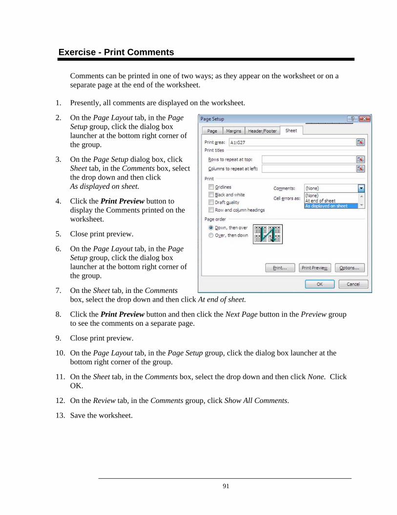
91

Exercise - Print Comments

Comments can be printed in one of two ways; as they appear on the worksheet or on a separate page at the end of the worksheet.

1. Presently, all comments are displayed on the worksheet.

2. On the Page Layout tab, in the Page Setup group, click the dialog box launcher at the bottom right corner of the group.

3. On the Page Setup dialog box, click Sheet tab, in the Comments box, select the drop down and then click As displayed on sheet.

4. Click the Print Preview button to display the Comments printed on the worksheet.

5. Close print preview.


7. On the Sheet tab, in the Comments box, select the drop down and then click At end of sheet.

8. Click the Print Preview button and then click the Next Page button in the Preview group to see the comments on a separate page.

9. Close print preview.


11. On the Sheet tab, in the Comments box, select the drop down and then click None. Click OK.

12. On the Review tab, in the Comments group, click Show All Comments.


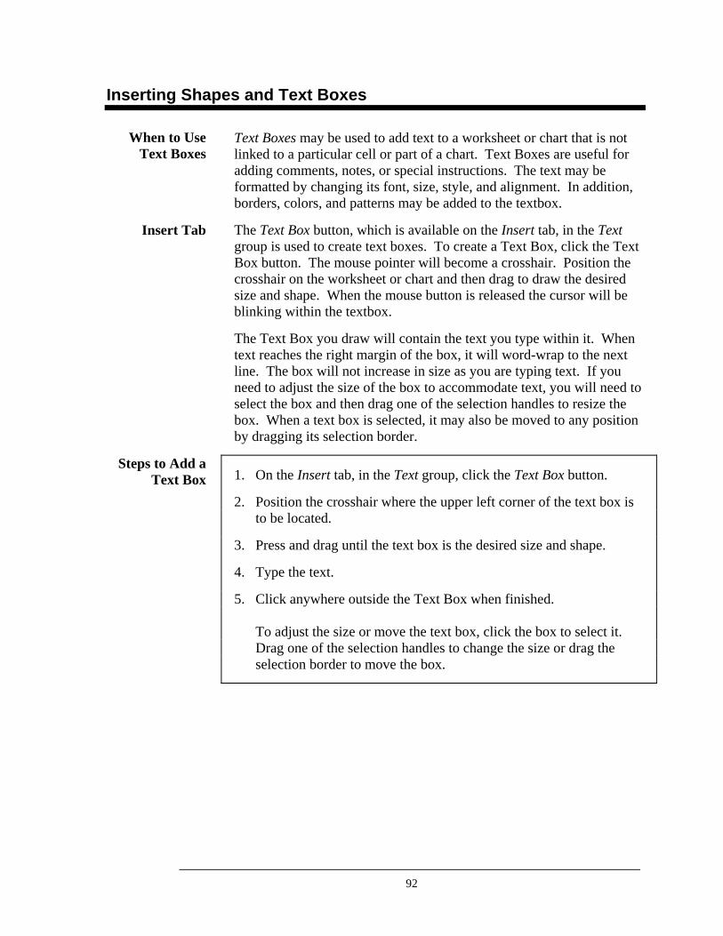
92

Inserting Shapes and Text Boxes

Text Boxes may be used to add text to a worksheet or chart that is not linked to a particular cell or part of a chart. Text Boxes are useful for adding comments, notes, or special instructions. The text may be formatted by changing its font, size, style, and alignment. In addition, borders, colors, and patterns may be added to the textbox.

The Text Box button, which is available on the Insert tab, in the Text group is used to create text boxes. To create a Text Box, click the Text Box button. The mouse pointer will become a crosshair. Position the crosshair on the worksheet or chart and then drag to draw the desired size and shape. When the mouse button is released the cursor will be blinking within the textbox.

The Text Box you draw will contain the text you type within it. When text reaches the right margin of the box, it will word-wrap to the next line. The box will not increase in size as you are typing text. If you need to adjust the size of the box to accommodate text, you will need to select the box and then drag one of the selection handles to resize the box. When a text box is selected, it may also be moved to any position by dragging its selection border.

1. On the Insert tab, in the Text group, click the Text Box button.

2. Position the crosshair where the upper left corner of the text box is to be located.

3. Press and drag until the text box is the desired size and shape.

4. Type the text.

5. Click anywhere outside the Text Box when finished. To adjust the size or move the text box, click the box to select it. Drag one of the selection handles to change the size or drag the selection border to move the box.

When to Use Text Boxes

Insert Tab

Steps to Add a Text Box

93

Exercise - Insert Text Boxes

To complete the 1st Quarter budget worksheet, you will draw an arrow and text box to insert a note about the quarterly balance.

1. Click the 1st Quarter sheet tab.

2. On the Insert tab, in the Text group, click the Text Box button.

3. Drag the crosshair to draw a text box that spans the range F19:G20.

4. Type: Good News! Ended the quarter with money left! Click outside the box when finished typing.

5. Click the text box to select it; then drag the mouse through the text to select it. On the Home tab, in the Font group, use buttons to bold the text and change the size to 12 point.

If the text box is not big enough to accommodate the text, enlarge it. Click on it to display the selection handles. Position the pointer arrow on a selection handle and then press and drag.

6. With the text box selected click the Fill color button and select a color.

7. Highlight the text. Select the Text Color button to select a color to complement the fill.

8. Right-click the textbox and then click Format Shape.

9. Click the Shadow category and then click the down-arrow on the Presets button. Select an Outer shadow. Click Close.

94

Exercise – Insert Shapes

1. On the Insert tab, in the Illustrations group, click the Shapes button.

2. Click the Arrow button. The mouse pointer switches to a crosshair.

3. Position the crosshair at the center, left edge of the text box you drew in the previous exercise.

4. Drag to the left to draw an arrow pointing to the value in Cell D19.

5. The Drawing Tools Format tab is now active. In the Shape Styles group, click Shape Outline and then point to Arrows. Click Arrow Style 5.

6. Click the Arrow. Click Shape Outline and then point to Weight. Click 3pt.

7. With the Arrow still selected, click the More button in the Shape Styles group to open Line Styles gallery. Select Intense Line Accent 2 from the bottom row.


95

Notes

96

Freeze Panes

When scrolling in large worksheets, it may be helpful to freeze the worksheet titles, so that no matter how far down or how far to the right you scroll, the worksheet titles will always be visible. You may choose to freeze horizontal or vertical titles only or to freeze both horizontal and vertical titles.

1. To freeze horizontal titles only, select the row below the titles. To freeze vertical titles only, select the column to the right of the titles. To freeze both horizontal and vertical titles, select the cell which is immediately below the horizontal titles and also immediately to the right of the vertical titles. (All rows above the selected cell and all columns to the left of the selected cell will be frozen.)

2. From the View tab, in the Window group, select Freeze Panes.

From the View tab, in the Window group, select Unfreeze Panes. (It does not matter which cell you have selected.)

Freeze Worksheet Titles

Freeze Titles

Unfreeze Titles

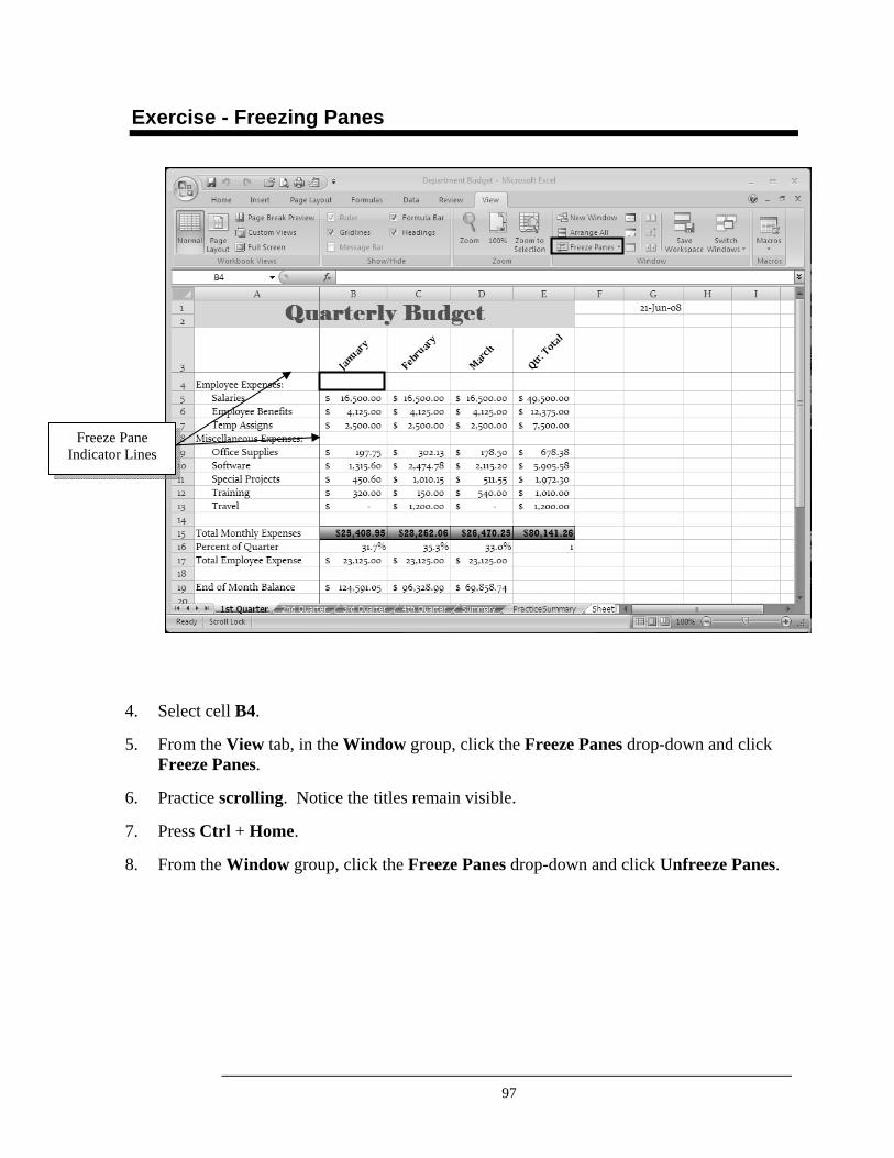
97

Exercise - Freezing Panes

4. Select cell B4.

5. From the View tab, in the Window group, click the Freeze Panes drop-down and click Freeze Panes.

6. Practice scrolling. Notice the titles remain visible.

7. Press Ctrl + Home.

8. From the Window group, click the Freeze Panes drop-down and click Unfreeze Panes.

Freeze Pane Indicator Lines

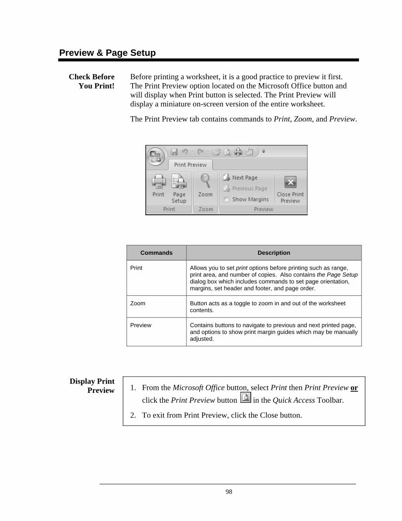
98

Preview & Page Setup

Before printing a worksheet, it is a good practice to preview it first. The Print Preview option located on the Microsoft Office button and will display when Print button is selected. The Print Preview will display a miniature on-screen version of the entire worksheet.

The Print Preview tab contains commands to Print, Zoom, and Preview.

Commands Description

Print Allows you to set print options before printing such as range, print area, and number of copies. Also contains the Page Setup dialog box which includes commands to set page orientation, margins, set header and footer, and page order.

Zoom Button acts as a toggle to zoom in and out of the worksheet contents.

Preview Contains buttons to navigate to previous and next printed page, and options to show print margin guides which may be manually adjusted.

1. From the Microsoft Office button, select Print then Print Preview or click the Print Preview button in the Quick Access Toolbar.

2. To exit from Print Preview, click the Close button.

Check Before You Print!

Display Print Preview

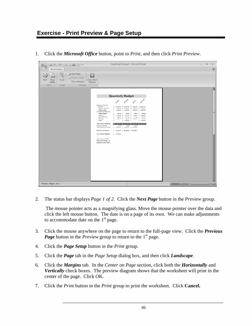
99

Exercise - Print Preview & Page Setup

1. Click the Microsoft Office button, point to Print, and then click Print Preview.

2. The status bar displays Page 1 of 2. Click the Next Page button in the Preview group.

The mouse pointer acts as a magnifying glass. Move the mouse pointer over the data and click the left mouse button. The date is on a page of its own. We can make adjustments to accommodate date on the 1st page.

3. Click the mouse anywhere on the page to return to the full-page view. Click the Previous Page button in the Preview group to return to the 1st page.

4. Click the Page Setup button in the Print group.

5. Click the Page tab in the Page Setup dialog box, and then click Landscape.

6. Click the Margins tab. In the Center on Page section, click both the Horizontally and Vertically check boxes. The preview diagram shows that the worksheet will print in the center of the page. Click OK.

7. Click the Print button in the Print group to print the worksheet. Click Cancel.

100

Headers and Footers (Print Preview & Page Setup)

Header information prints at the top of every page of a worksheet. Footer information prints at the bottom of every page. To access the header and footer dialog boxes, select Page Setup from the Print group on the Print Preview tab and then click the Header/Footer tab. To enhance the professional appearance of a worksheet, you may select from built-in headers/footers or type your own custom headers/footers .

1. On the Print Preview tab, in the Print group select Page Setup.

2. Select the Header/Footer tab.

3. Select a built-in header or footer from the header or footer drop down-list boxes. OR

4. Click the Custom Header or Custom Footer button. The header or footer dialog box will be displayed.

5. Enter the header/footer information in the Left, Center, and Right sections. Ten buttons are provided to insert special options.

Format Text button used to format the selected text in the text boxes; when using this font button, the text must be selected first; when this button is clicked, the font dialog box displays.

Page number button; inserts the code to print the page number

Number of total pages button; inserts the code to print the page number out of the total number of pages

Date button; inserts the code to print the computer's current date

Time button; inserts the code to print the computer's current time

File Path button; inserts path to the location of the file

Filename button; inserts the code to print the worksheet's filename

Sheet name , inserts the code to print the worksheet tab name

Image button; inserts an image

Format picture; change size and characteristics of the image

6. Click OK.

Headers and Footers

Steps to Create Header/Footer

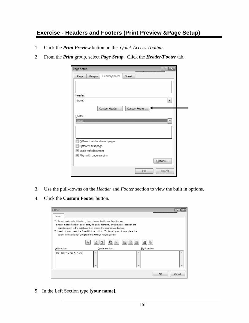
101

Exercise - Headers and Footers (Print Preview &Page Setup)

1. Click the Print Preview button on the Quick Access Toolbar.

2. From the Print group, select Page Setup. Click the Header/Footer tab.

3. Use the pull-downs on the Header and Footer section to view the built in options.

4. Click the Custom Footer button.

5. In the Left Section type [your name].

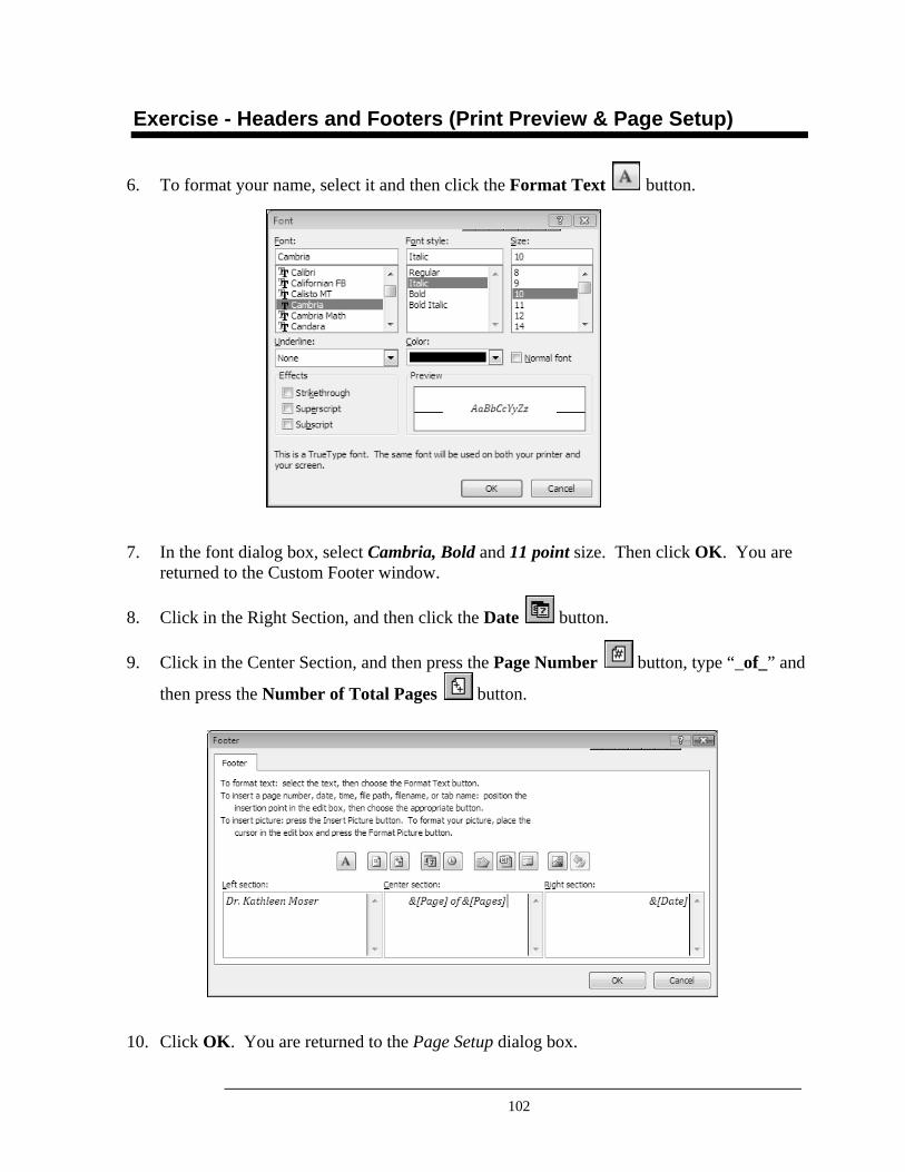
102

Exercise - Headers and Footers (Print Preview & Page Setup)

6. To format your name, select it and then click the Format Text button.

7. In the font dialog box, select Cambria, Bold and 11 point size. Then click OK. You are returned to the Custom Footer window.

8. Click in the Right Section, and then click the Date button.

9. Click in the Center Section, and then press the Page Number button, type “_of_” and

then press the Number of Total Pages button.

10. Click OK. You are returned to the Page Setup dialog box.

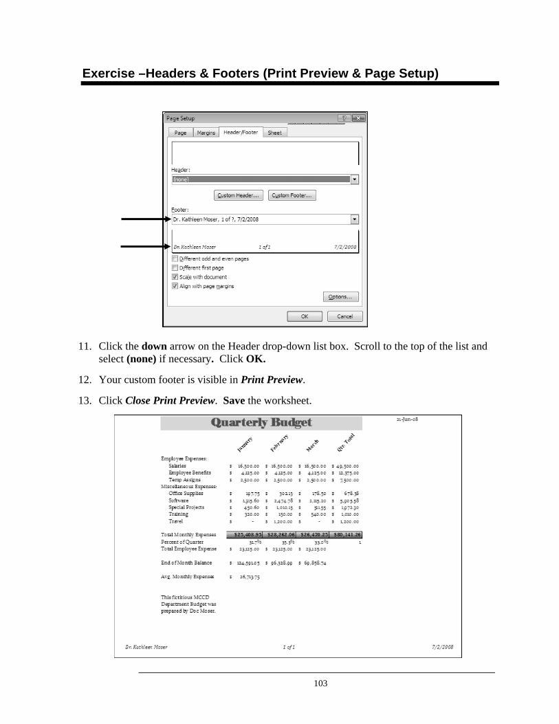
103

Exercise –Headers & Footers (Print Preview & Page Setup)

11. Click the down arrow on the Header drop-down list box. Scroll to the top of the list and

select (none) if necessary. Click OK.

12. Your custom footer is visible in Print Preview.

13. Click Close Print Preview. Save the worksheet.

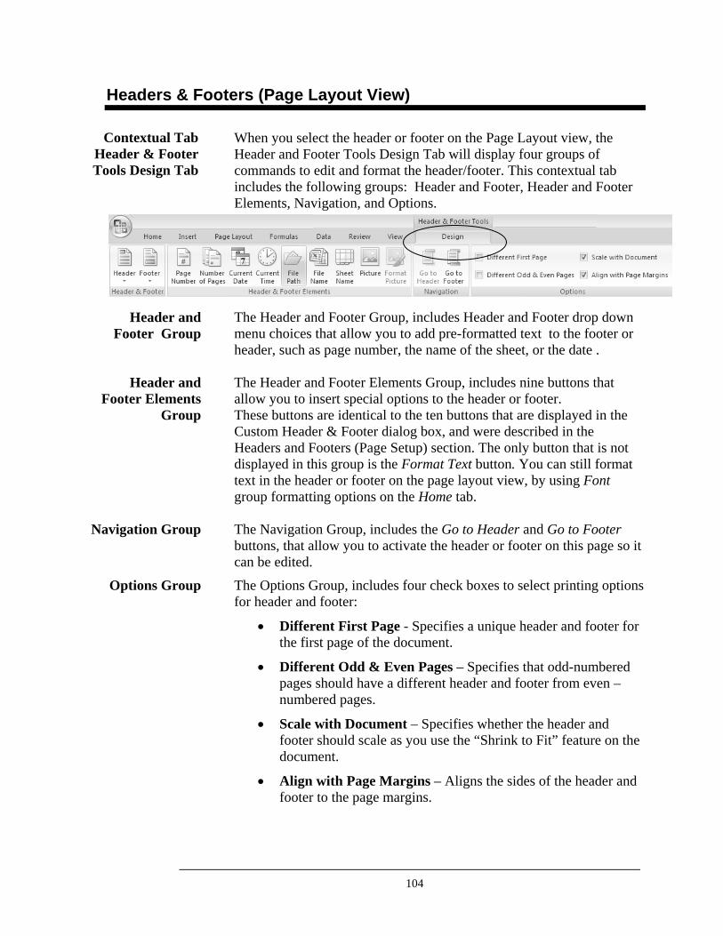
104

Headers & Footers (Page Layout View)

When you select the header or footer on the Page Layout view, the Header and Footer Tools Design Tab will display four groups of commands to edit and format the header/footer. This contextual tab includes the following groups: Header and Footer, Header and Footer Elements, Navigation, and Options. The Header and Footer Group, includes Header and Footer drop down menu choices that allow you to add pre-formatted text to the footer or header, such as page number, the name of the sheet, or the date . The Header and Footer Elements Group, includes nine buttons that allow you to insert special options to the header or footer. These buttons are identical to the ten buttons that are displayed in the Custom Header & Footer dialog box, and were described in the Headers and Footers (Page Setup) section. The only button that is not displayed in this group is the Format Text button. You can still format text in the header or footer on the page layout view, by using Font group formatting options on the Home tab. The Navigation Group, includes the Go to Header and Go to Footer buttons, that allow you to activate the header or footer on this page so it can be edited.

The Options Group, includes four check boxes to select printing options for header and footer:

• Different First Page - Specifies a unique header and footer for the first page of the document.

• Different Odd & Even Pages – Specifies that odd-numbered pages should have a different header and footer from even –numbered pages.

• Scale with Document – Specifies whether the header and footer should scale as you use the “Shrink to Fit” feature on the document.

• Align with Page Margins – Aligns the sides of the header and footer to the page margins.

Contextual Tab Header & Footer Tools Design Tab

Header and Footer Group

Header and Footer Elements

Group

Navigation Group

Options Group

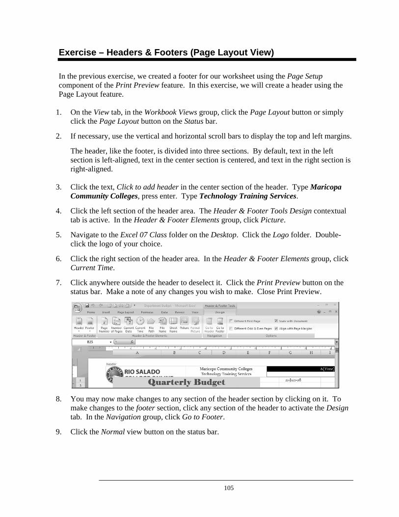
105

Exercise – Headers & Footers (Page Layout View)

In the previous exercise, we created a footer for our worksheet using the Page Setup component of the Print Preview feature. In this exercise, we will create a header using the Page Layout feature.

1. On the View tab, in the Workbook Views group, click the Page Layout button or simply click the Page Layout button on the Status bar.

2. If necessary, use the vertical and horizontal scroll bars to display the top and left margins.

The header, like the footer, is divided into three sections. By default, text in the left section is left-aligned, text in the center section is centered, and text in the right section is right-aligned.

3. Click the text, Click to add header in the center section of the header. Type Maricopa Community Colleges, press enter. Type Technology Training Services.

4. Click the left section of the header area. The Header & Footer Tools Design contextual tab is active. In the Header & Footer Elements group, click Picture.

5. Navigate to the Excel 07 Class folder on the Desktop. Click the Logo folder. Double-click the logo of your choice.

6. Click the right section of the header area. In the Header & Footer Elements group, click Current Time.

7. Click anywhere outside the header to deselect it. Click the Print Preview button on the status bar. Make a note of any changes you wish to make. Close Print Preview.

8. You may now make changes to any section of the header section by clicking on it. To make changes to the footer section, click any section of the header to activate the Design tab. In the Navigation group, click Go to Footer.

9. Click the Normal view button on the status bar.

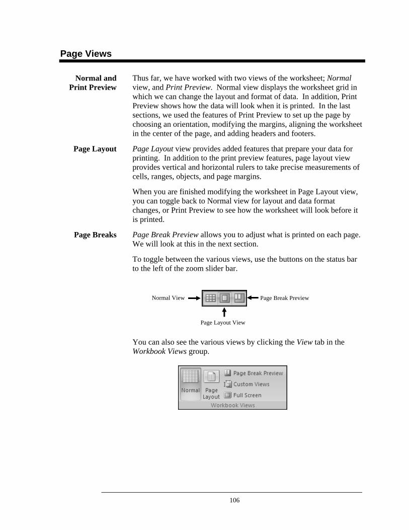
106

Page Views

Thus far, we have worked with two views of the worksheet; Normal view, and Print Preview. Normal view displays the worksheet grid in which we can change the layout and format of data. In addition, Print Preview shows how the data will look when it is printed. In the last sections, we used the features of Print Preview to set up the page by choosing an orientation, modifying the margins, aligning the worksheet in the center of the page, and adding headers and footers.

Page Layout view provides added features that prepare your data for printing. In addition to the print preview features, page layout view provides vertical and horizontal rulers to take precise measurements of cells, ranges, objects, and page margins.

When you are finished modifying the worksheet in Page Layout view, you can toggle back to Normal view for layout and data format changes, or Print Preview to see how the worksheet will look before it is printed.

Page Break Preview allows you to adjust what is printed on each page. We will look at this in the next section.

To toggle between the various views, use the buttons on the status bar to the left of the zoom slider bar.

You can also see the various views by clicking the View tab in the Workbook Views group.

Normal and Print Preview

Page Layout

Page Breaks

Normal View Page Break Preview

Page Layout View

107

Notes

108

Page Break Preview

If after you have completed your Page Setup, you still cannot get your spreadsheet to appear correctly on your page, you can try using the Page Break Preview. The Page Break Preview allows you to edit where your page(s) will end and begin. Excel will automatically adjust the size of your spreadsheet to fit on the page when you print. This will help to prevent one column or row from spilling onto the next page and wasting paper. Page Break Preview is under the View tab, Workbook Views group or on the status bar next to the zoom slider bar.

1. Click the View tab, Workbook Views group Page Break Preview button or the Page Break Preview button on the status bar next to the zoom slider bar.

2. Click on the blue page lines and adjust the pages to required size .

3. To return to normal view, click the Normal view button on the status bar.

Why Use Page Break Preview?

Steps to Use Page Break Preview

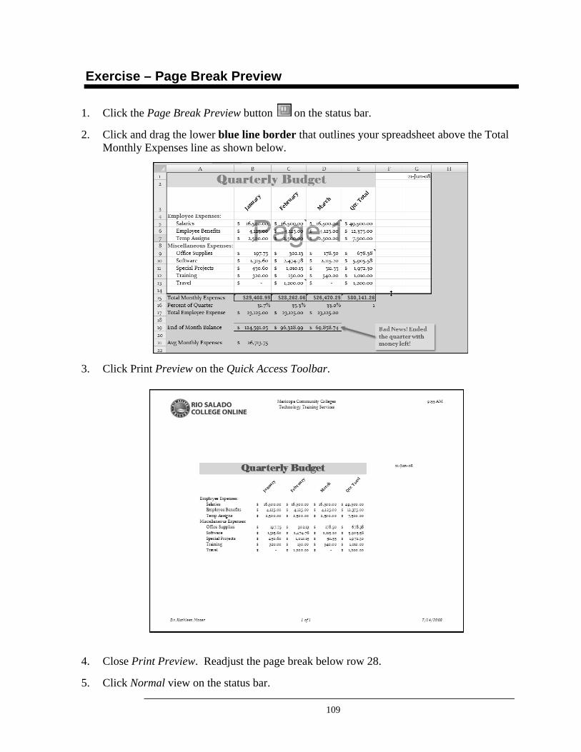
109

Exercise – Page Break Preview

1. Click the Page Break Preview button on the status bar.

2. Click and drag the lower blue line border that outlines your spreadsheet above the Total Monthly Expenses line as shown below.

3. Click Print Preview on the Quick Access Toolbar.

4. Close Print Preview. Readjust the page break below row 28.

5. Click Normal view on the status bar.

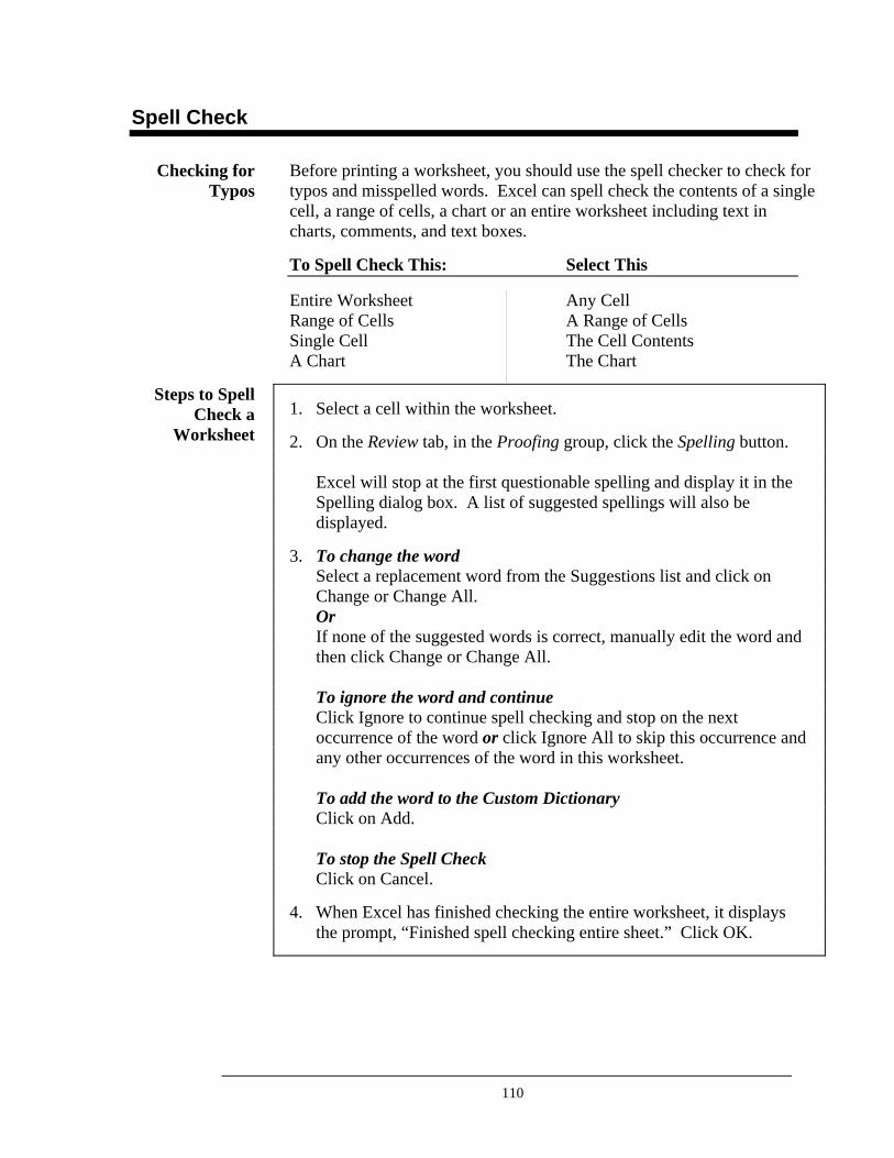
110

Spell Check

Before printing a worksheet, you should use the spell checker to check for typos and misspelled words. Excel can spell check the contents of a single cell, a range of cells, a chart or an entire worksheet including text in charts, comments, and text boxes.

To Spell Check This: Select This

Entire Worksheet Any Cell Range of Cells A Range of Cells Single Cell The Cell Contents A Chart The Chart

1. Select a cell within the worksheet.

2. On the Review tab, in the Proofing group, click the Spelling button. Excel will stop at the first questionable spelling and display it in the Spelling dialog box. A list of suggested spellings will also be displayed.

3. To change the word Select a replacement word from the Suggestions list and click on Change or Change All. Or If none of the suggested words is correct, manually edit the word and then click Change or Change All. To ignore the word and continue Click Ignore to continue spell checking and stop on the next occurrence of the word or click Ignore All to skip this occurrence and any other occurrences of the word in this worksheet. To add the word to the Custom Dictionary Click on Add. To stop the Spell Check Click on Cancel.

4. When Excel has finished checking the entire worksheet, it displays the prompt, “Finished spell checking entire sheet.” Click OK.

Checking for Typos

Steps to Spell Check a

Worksheet

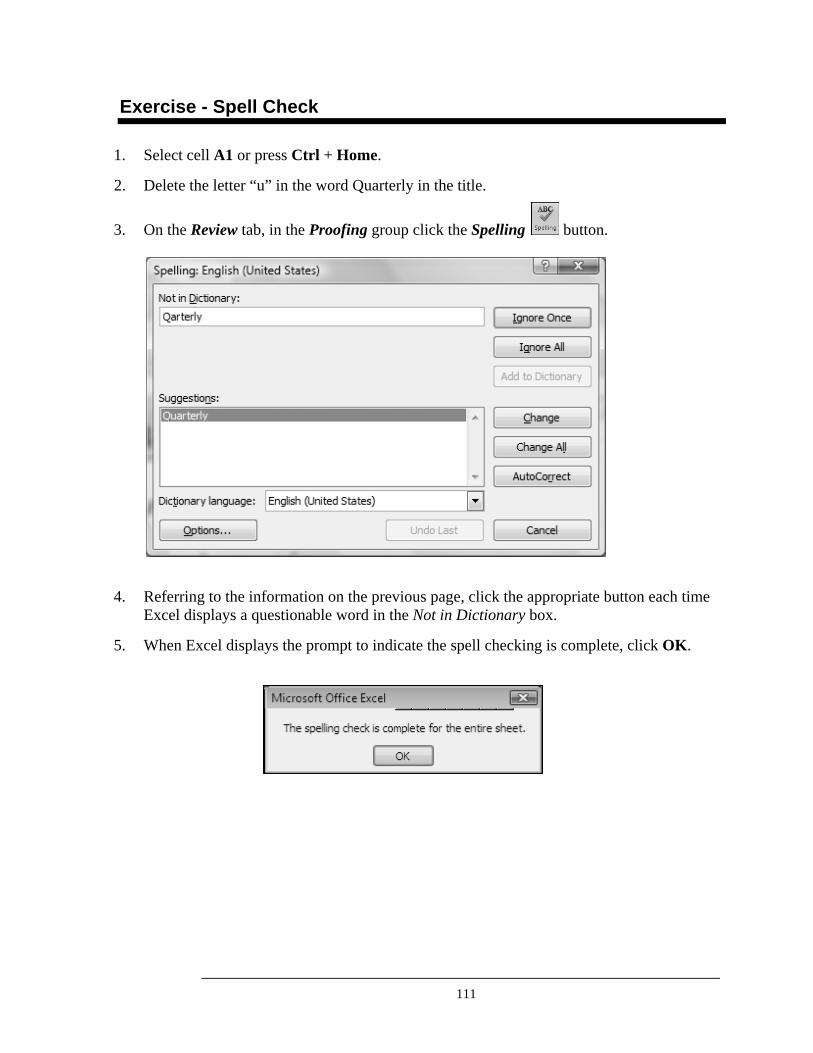
111

Exercise - Spell Check

1. Select cell A1 or press Ctrl + Home.

2. Delete the letter “u” in the word Quarterly in the title.

3. On the Review tab, in the Proofing group click the Spelling button.

4. Referring to the information on the previous page, click the appropriate button each time Excel displays a questionable word in the Not in Dictionary box.

5. When Excel displays the prompt to indicate the spell checking is complete, click OK.

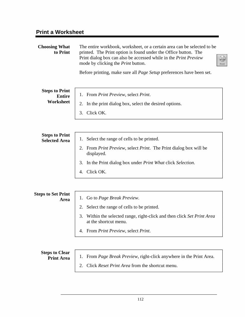
112

Print a Worksheet

The entire workbook, worksheet, or a certain area can be selected to be printed. The Print option is found under the Office button. The Print dialog box can also be accessed while in the Print Preview mode by clicking the Print button.

Before printing, make sure all Page Setup preferences have been set.

1. From Print Preview, select Print.

2. In the print dialog box, select the desired options.

3. Click OK.

1. Select the range of cells to be printed.

2. From Print Preview, select Print. The Print dialog box will be displayed.

3. In the Print dialog box under Print What click Selection.

4. Click OK.

1. Go to Page Break Preview.

2. Select the range of cells to be printed.

3. Within the selected range, right-click and then click Set Print Area at the shortcut menu.

4. From Print Preview, select Print.

1. From Page Break Preview, right-click anywhere in the Print Area.

2. Click Reset Print Area from the shortcut menu.

Choosing What to Print

Steps to Print Entire

Worksheet

Steps to Print Selected Area

Steps to Set Print Area

Steps to Clear Print Area

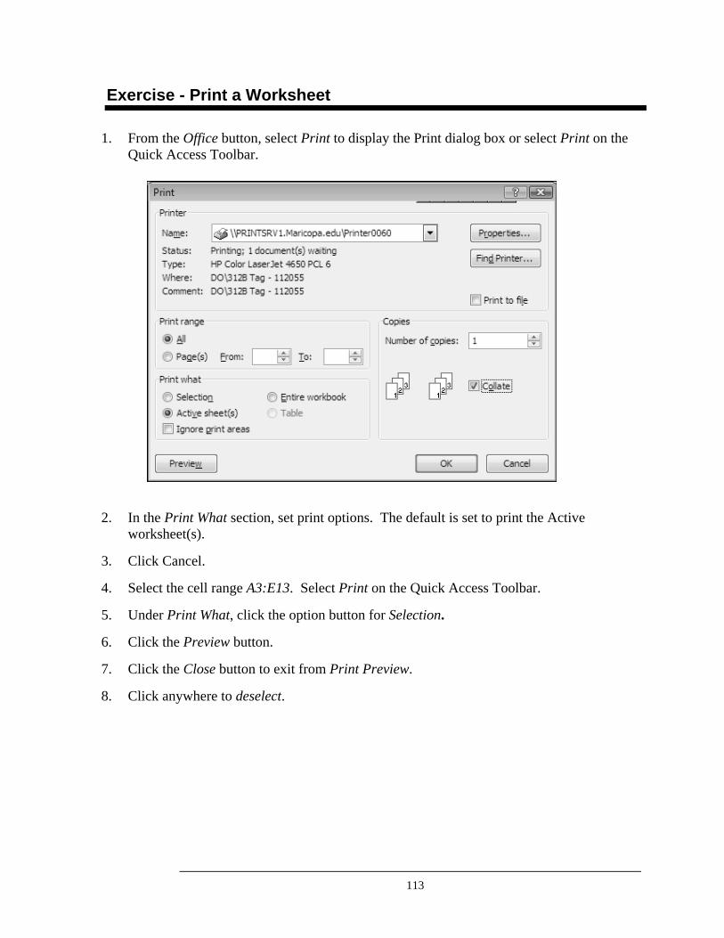
113

Exercise - Print a Worksheet

1. From the Office button, select Print to display the Print dialog box or select Print on the Quick Access Toolbar.

2. In the Print What section, set print options. The default is set to print the Active worksheet(s).

3. Click Cancel.

4. Select the cell range A3:E13. Select Print on the Quick Access Toolbar.

5. Under Print What, click the option button for Selection.

6. Click the Preview button.

7. Click the Close button to exit from Print Preview.


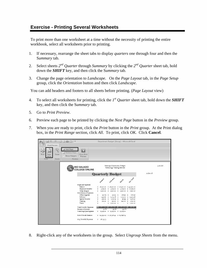
114

Exercise - Printing Several Worksheets

To print more than one worksheet at a time without the necessity of printing the entire workbook, select all worksheets prior to printing.

1. If necessary, rearrange the sheet tabs to display quarters one through four and then the Summary tab.

2. Select sheets 2nd Quarter through Summary by clicking the 2nd Quarter sheet tab, hold down the SHIFT key, and then click the Summary tab.

3. Change the page orientation to Landscape. On the Page Layout tab, in the Page Setup group, click the Orientation button and then click Landscape.

You can add headers and footers to all sheets before printing. (Page Layout view)

4. To select all worksheets for printing, click the 1st Quarter sheet tab, hold down the SHIFT key, and then click the Summary tab.

5. Go to Print Preview.

6. Preview each page to be printed by clicking the Next Page button in the Preview group.

7. When you are ready to print, click the Print button in the Print group. At the Print dialog box, in the Print Range section, click All. To print, click OK. Click Cancel.

8. Right-click any of the worksheets in the group. Select Ungroup Sheets from the menu.

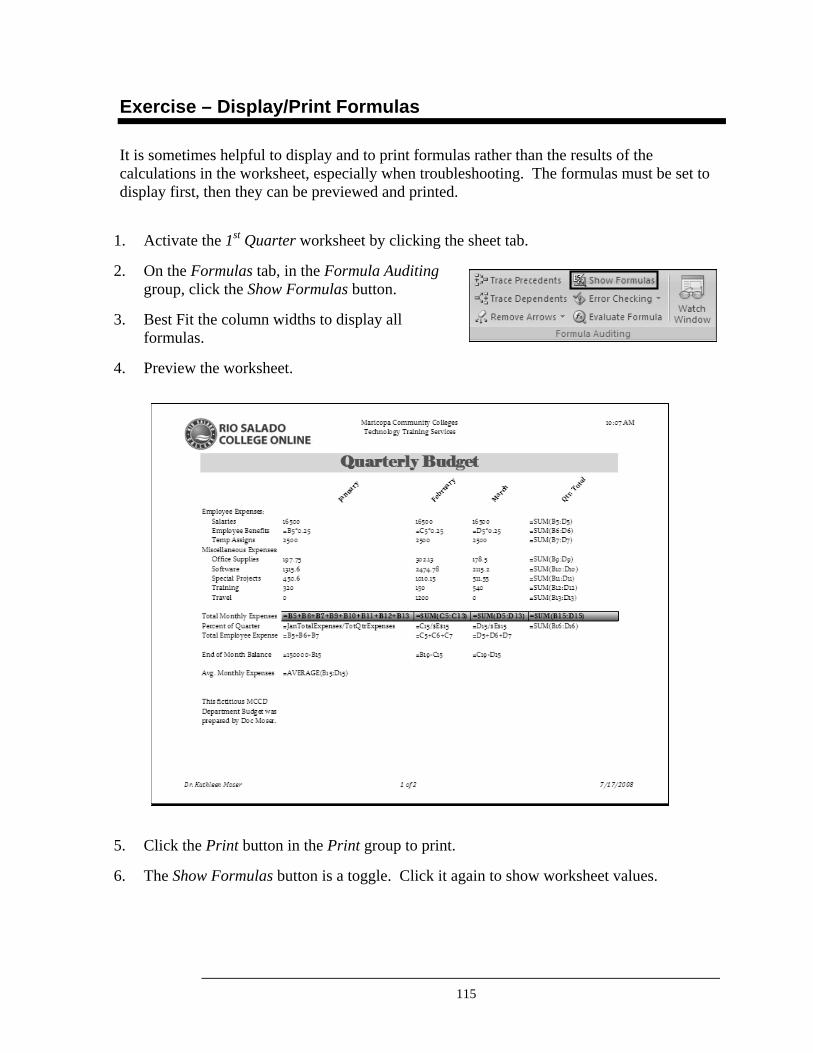
115

Exercise – Display/Print Formulas

It is sometimes helpful to display and to print formulas rather than the results of the calculations in the worksheet, especially when troubleshooting. The formulas must be set to display first, then they can be previewed and printed.

1. Activate the 1st Quarter worksheet by clicking the sheet tab.

2. On the Formulas tab, in the Formula Auditing group, click the Show Formulas button.

3. Best Fit the column widths to display all formulas.

4. Preview the worksheet.

5. Click the Print button in the Print group to print.

6. The Show Formulas button is a toggle. Click it again to show worksheet values.

116

What- If Analysis

Once your worksheet has been completed with formulas, you can use what-if scenarios to explore various results. What-if analysis is the process of changing the values in your worksheet to see how those changes will affect the outcome of your results. For example, you can calculate a best and worst case scenario for your quarterly budget by adding and subtracting expenditures in various categories. Excel will automatically recalculate and display new projected values in all cells that have formulas affected by the change.

You will want to save a copy of the worksheet before performing the projections so that the original worksheet will remain untouched. In the example above, you would preserve your budget worksheet unchanged and create a new one for the “what if” projections. To save a copy, click the Microsoft Office button and then click Save As.

1. Select the cell(s) requiring the change and enter the new value(s).

2. Excel will automatically recalculate and display the new projected values in all cells that have formulas affected by the change.

“What If” Analysis

Tip

Make Projections

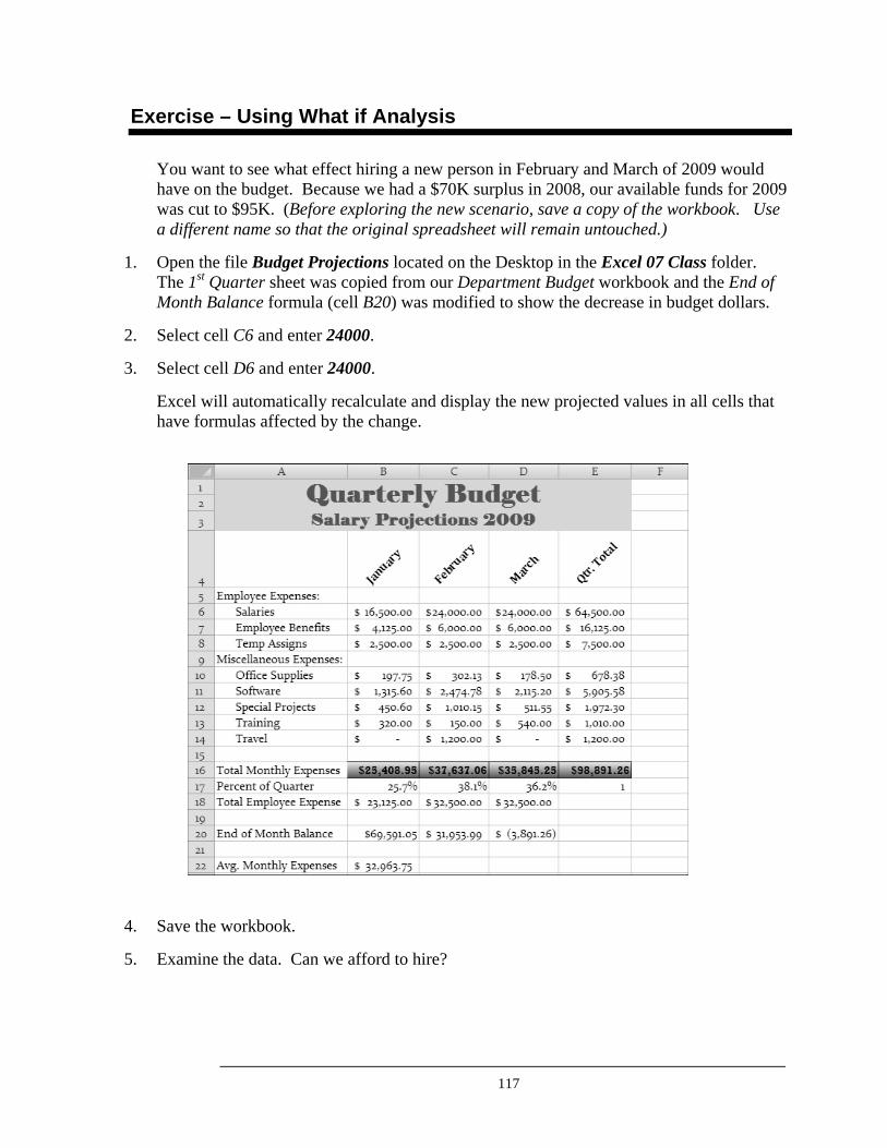
117

Exercise – Using What if Analysis

You want to see what effect hiring a new person in February and March of 2009 would have on the budget. Because we had a $70K surplus in 2008, our available funds for 2009 was cut to $95K. (Before exploring the new scenario, save a copy of the workbook. Use a different name so that the original spreadsheet will remain untouched.)

1. Open the file Budget Projections located on the Desktop in the Excel 07 Class folder. The 1st Quarter sheet was copied from our Department Budget workbook and the End of Month Balance formula (cell B20) was modified to show the decrease in budget dollars.

2. Select cell C6 and enter 24000.

3. Select cell D6 and enter 24000.

Excel will automatically recalculate and display the new projected values in all cells that have formulas affected by the change.


5. Examine the data. Can we afford to hire?

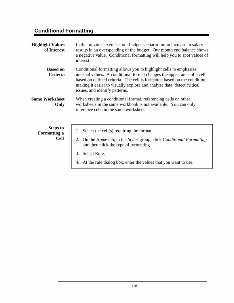
118

Conditional Formatting

In the previous exercise, our budget scenario for an increase in salary results in an overspending of the budget. Our month end balance shows a negative value. Conditional formatting will help you to spot values of interest.

Conditional formatting allows you to highlight cells to emphasize unusual values. A conditional format changes the appearance of a cell based on defined criteria. The cell is formatted based on the condition, making it easier to visually explore and analyze data, detect critical issues, and identify patterns.

When creating a conditional format, referencing cells on other worksheets in the same workbook is not available. You can only reference cells in the same worksheet.

1. Select the cell(s) requiring the format

2. On the Home tab, in the Styles group, click Conditional Formatting and then click the type of formatting.

3. Select Rule.

4. At the rule dialog box, enter the values that you want to use.

Highlight Values of Interest

Based on Criteria

Same Worksheet Only

Steps to Formatting a

Cell

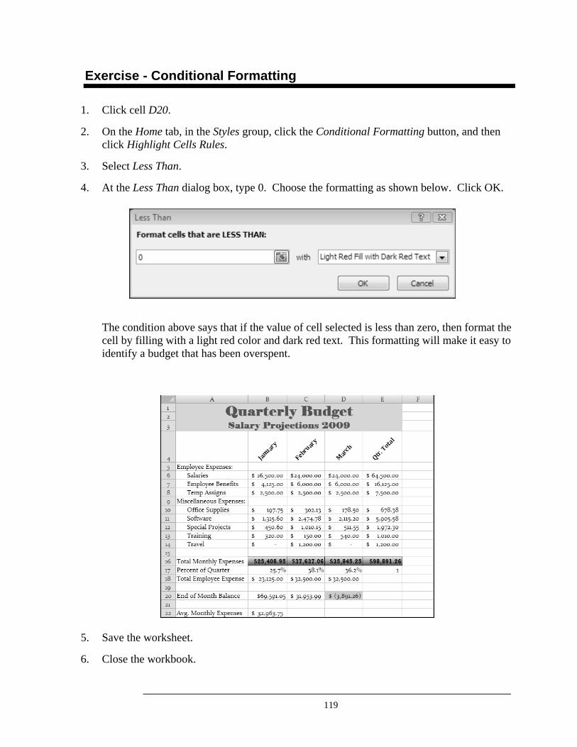
119

Exercise - Conditional Formatting

1. Click cell D20.

2. On the Home tab, in the Styles group, click the Conditional Formatting button, and then click Highlight Cells Rules.

3. Select Less Than.

4. At the Less Than dialog box, type 0. Choose the formatting as shown below. Click OK.

The condition above says that if the value of cell selected is less than zero, then format the cell by filling with a light red color and dark red text. This formatting will make it easy to identify a budget that has been overspent.


6. Close the workbook.

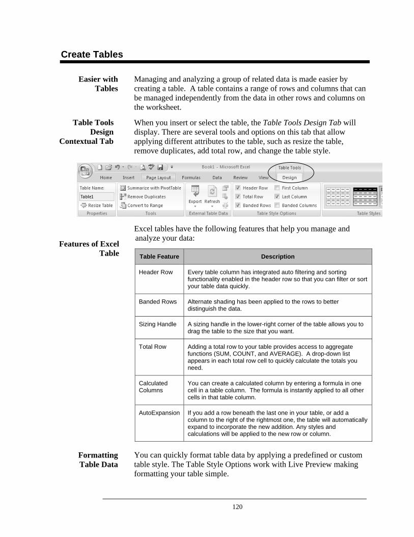
120

Create Tables

Managing and analyzing a group of related data is made easier by creating a table. A table contains a range of rows and columns that can be managed independently from the data in other rows and columns on the worksheet.

When you insert or select the table, the Table Tools Design Tab will display. There are several tools and options on this tab that allow applying different attributes to the table, such as resize the table, remove duplicates, add total row, and change the table style. Excel tables have the following features that help you manage and analyze your data:

Table Feature Description

Header Row Every table column has integrated auto filtering and sorting functionality enabled in the header row so that you can filter or sort your table data quickly.

Banded Rows Alternate shading has been applied to the rows to better distinguish the data.

Sizing Handle A sizing handle in the lower-right corner of the table allows you to drag the table to the size that you want.

Total Row Adding a total row to your table provides access to aggregate functions (SUM, COUNT, and AVERAGE). A drop-down list appears in each total row cell to quickly calculate the totals you need.

Calculated Columns

You can create a calculated column by entering a formula in one cell in a table column. The formula is instantly applied to all other cells in that table column.

AutoExpansion If you add a row beneath the last one in your table, or add a column to the right of the rightmost one, the table will automatically expand to incorporate the new addition. Any styles and calculations will be applied to the new row or column.

You can quickly format table data by applying a predefined or custom table style. The Table Style Options work with Live Preview making formatting your table simple.

Easier with Tables

Table Tools Design

Contextual Tab

Features of Excel Table

Formatting Table Data

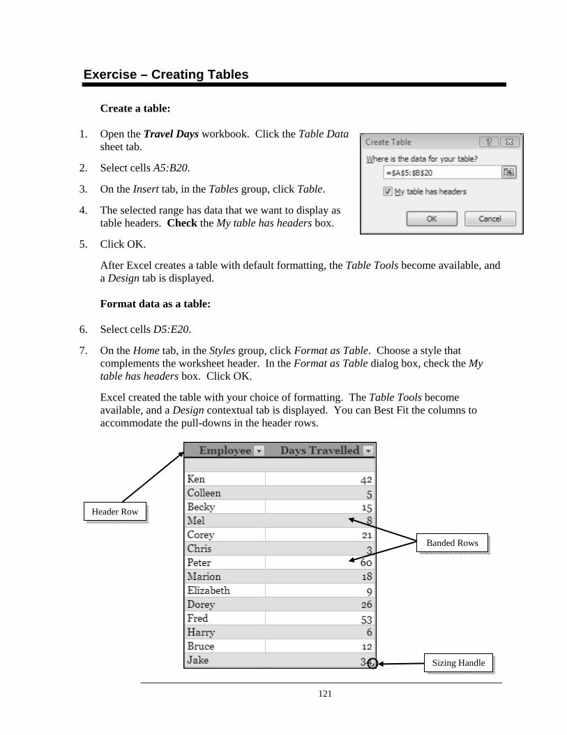
121

Exercise – Creating Tables

Create a table:

1. Open the Travel Days workbook. Click the Table Data sheet tab.

2. Select cells A5:B20.

3. On the Insert tab, in the Tables group, click Table.

4. The selected range has data that we want to display as table headers. Check the My table has headers box.

5. Click OK.

After Excel creates a table with default formatting, the Table Tools become available, and a Design tab is displayed. Format data as a table:

6. Select cells D5:E20.

7. On the Home tab, in the Styles group, click Format as Table. Choose a style that complements the worksheet header. In the Format as Table dialog box, check the My table has headers box. Click OK.

Excel created the table with your choice of formatting. The Table Tools become available, and a Design contextual tab is displayed. You can Best Fit the columns to accommodate the pull-downs in the header rows.

Header Row

Banded Rows

Sizing Handle

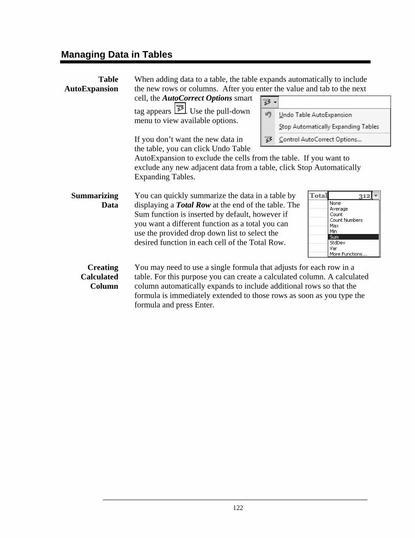
122

Managing Data in Tables

When adding data to a table, the table expands automatically to include the new rows or columns. After you enter the value and tab to the next cell, the AutoCorrect Options smart tag appears . Use the pull-down menu to view available options. If you don’t want the new data in the table, you can click Undo Table AutoExpansion to exclude the cells from the table. If you want to exclude any new adjacent data from a table, click Stop Automatically Expanding Tables. You can quickly summarize the data in a table by displaying a Total Row at the end of the table. The Sum function is inserted by default, however if you want a different function as a total you can use the provided drop down list to select the desired function in each cell of the Total Row.

You may need to use a single formula that adjusts for each row in a table. For this purpose you can create a calculated column. A calculated column automatically expands to include additional rows so that the formula is immediately extended to those rows as soon as you type the formula and press Enter.

Table AutoExpansion

Summarizing Data

Creating Calculated

Column

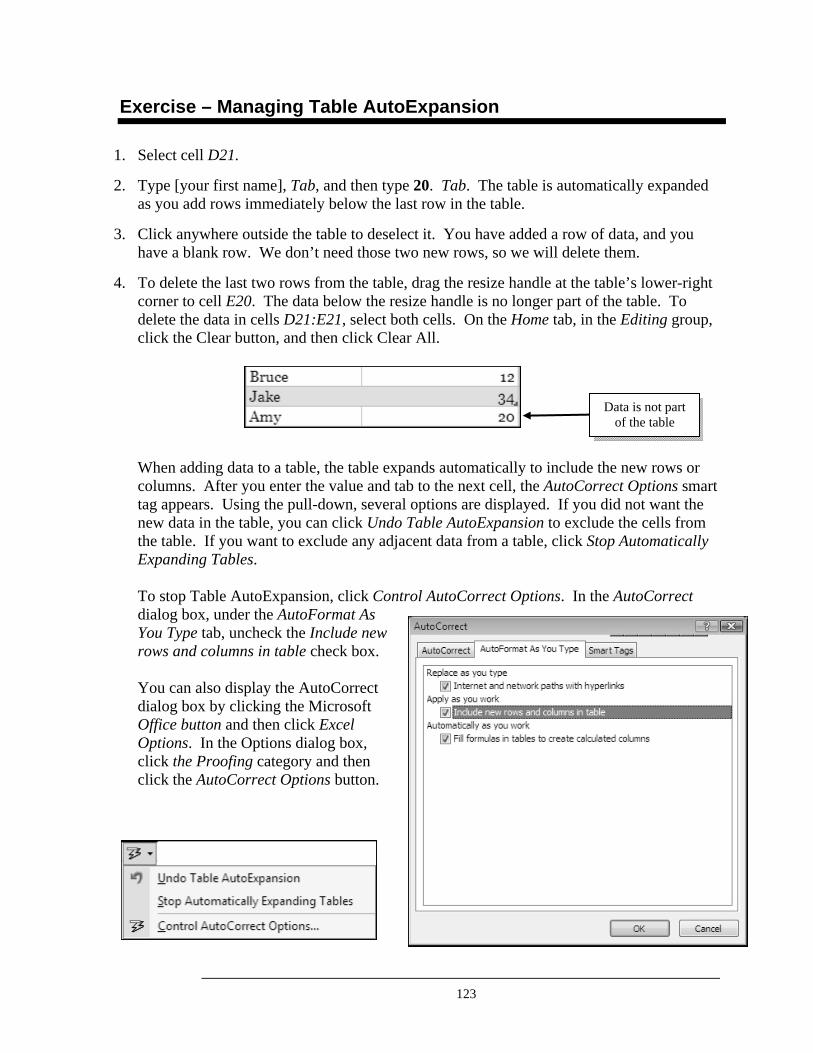
123

Exercise – Managing Table AutoExpansion

1. Select cell D21.

2. Type [your first name], Tab, and then type 20. Tab. The table is automatically expanded as you add rows immediately below the last row in the table.

3. Click anywhere outside the table to deselect it. You have added a row of data, and you have a blank row. We don’t need those two new rows, so we will delete them.

4. To delete the last two rows from the table, drag the resize handle at the table’s lower-right corner to cell E20. The data below the resize handle is no longer part of the table. To delete the data in cells D21:E21, select both cells. On the Home tab, in the Editing group, click the Clear button, and then click Clear All.

When adding data to a table, the table expands automatically to include the new rows or columns. After you enter the value and tab to the next cell, the AutoCorrect Options smart tag appears. Using the pull-down, several options are displayed. If you did not want the new data in the table, you can click Undo Table AutoExpansion to exclude the cells from the table. If you want to exclude any adjacent data from a table, click Stop Automatically Expanding Tables. To stop Table AutoExpansion, click Control AutoCorrect Options. In the AutoCorrect dialog box, under the AutoFormat As You Type tab, uncheck the Include new rows and columns in table check box. You can also display the AutoCorrect dialog box by clicking the Microsoft Office button and then click Excel Options. In the Options dialog box, click the Proofing category and then click the AutoCorrect Options button.

Data is not part of the table

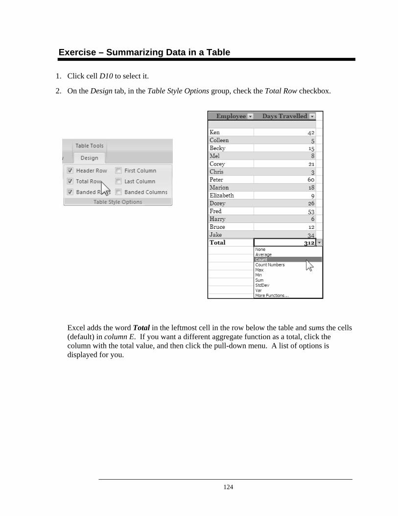
124

Exercise – Summarizing Data in a Table

1. Click cell D10 to select it.

2. On the Design tab, in the Table Style Options group, check the Total Row checkbox.

Excel adds the word Total in the leftmost cell in the row below the table and sums the cells (default) in column E. If you want a different aggregate function as a total, click the column with the total value, and then click the pull-down menu. A list of options is displayed for you.

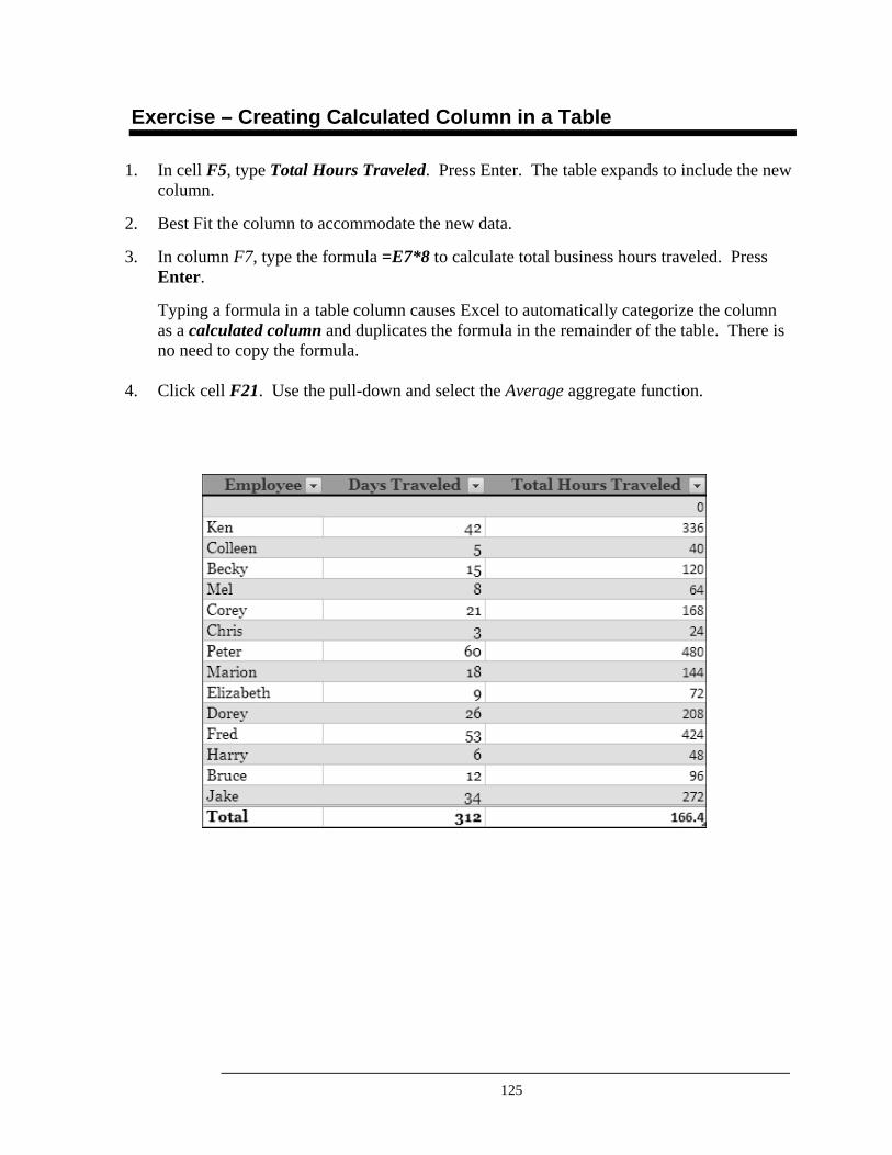
125

Exercise – Creating Calculated Column in a Table

1. In cell F5, type Total Hours Traveled. Press Enter. The table expands to include the new column.

2. Best Fit the column to accommodate the new data.

3. In column F7, type the formula =E7*8 to calculate total business hours traveled. Press Enter.

Typing a formula in a table column causes Excel to automatically categorize the column as a calculated column and duplicates the formula in the remainder of the table. There is no need to copy the formula.

4. Click cell F21. Use the pull-down and select the Average aggregate function.

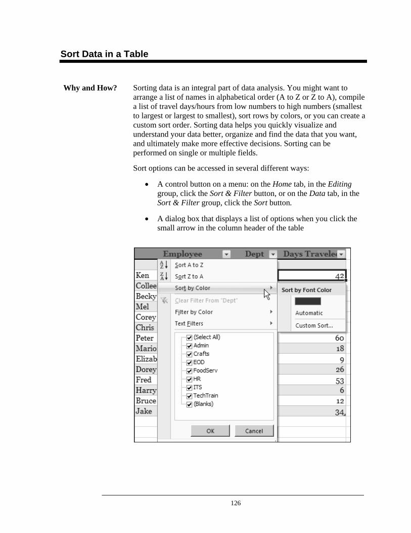
126

Sort Data in a Table

Sorting data is an integral part of data analysis. You might want to arrange a list of names in alphabetical order (A to Z or Z to A), compile a list of travel days/hours from low numbers to high numbers (smallest to largest or largest to smallest), sort rows by colors, or you can create a custom sort order. Sorting data helps you quickly visualize and understand your data better, organize and find the data that you want, and ultimately make more effective decisions. Sorting can be performed on single or multiple fields.

Sort options can be accessed in several different ways:

• A control button on a menu: on the Home tab, in the Editing group, click the Sort & Filter button, or on the Data tab, in the Sort & Filter group, click the Sort button.

• A dialog box that displays a list of options when you click the small arrow in the column header of the table

Why and How?

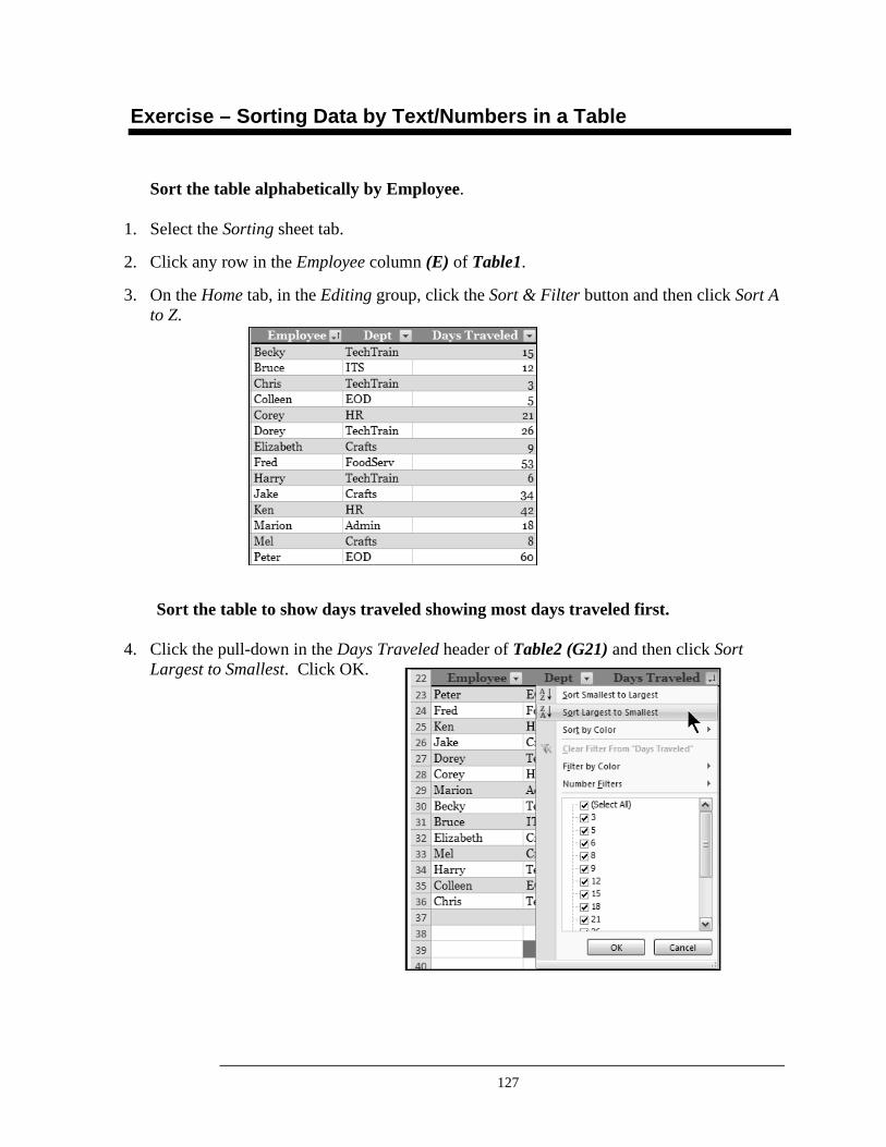
127

Exercise – Sorting Data by Text/Numbers in a Table

Sort the table alphabetically by Employee.

1. Select the Sorting sheet tab.

2. Click any row in the Employee column (E) of Table1.

3. On the Home tab, in the Editing group, click the Sort & Filter button and then click Sort A to Z.

Sort the table to show days traveled showing most days traveled first.

4. Click the pull-down in the Days Traveled header of Table2 (G21) and then click Sort Largest to Smallest. Click OK.

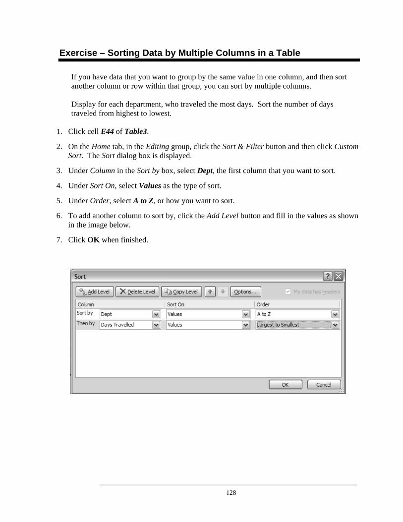
128

Exercise – Sorting Data by Multiple Columns in a Table

If you have data that you want to group by the same value in one column, and then sort another column or row within that group, you can sort by multiple columns. Display for each department, who traveled the most days. Sort the number of days traveled from highest to lowest.

1. Click cell E44 of Table3.

2. On the Home tab, in the Editing group, click the Sort & Filter button and then click Custom Sort. The Sort dialog box is displayed.

3. Under Column in the Sort by box, select Dept, the first column that you want to sort.

4. Under Sort On, select Values as the type of sort.

5. Under Order, select A to Z, or how you want to sort.

6. To add another column to sort by, click the Add Level button and fill in the values as shown in the image below.

7. Click OK when finished.

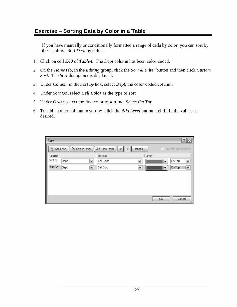
129

Exercise – Sorting Data by Color in a Table

If you have manually or conditionally formatted a range of cells by color, you can sort by these colors. Sort Dept by color.

1. Click on cell E60 of Table4. The Dept column has been color-coded.

2. On the Home tab, in the Editing group, click the Sort & Filter button and then click Custom Sort. The Sort dialog box is displayed.

3. Under Column in the Sort by box, select Dept, the color-coded column.

4. Under Sort On, select Cell Color as the type of sort.

5. Under Order, select the first color to sort by. Select On Top.

6. To add another column to sort by, click the Add Level button and fill in the values as desired.

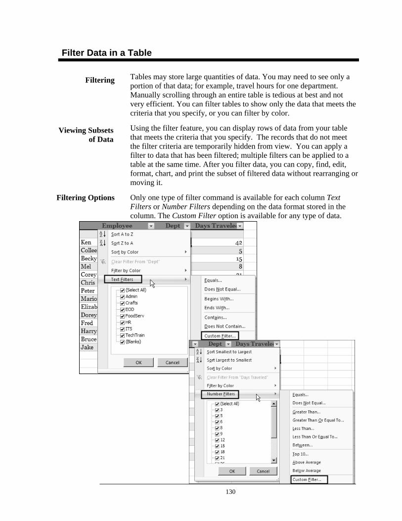
130

Filter Data in a Table

Tables may store large quantities of data. You may need to see only a portion of that data; for example, travel hours for one department. Manually scrolling through an entire table is tedious at best and not very efficient. You can filter tables to show only the data that meets the criteria that you specify, or you can filter by color.

Using the filter feature, you can display rows of data from your table that meets the criteria that you specify. The records that do not meet the filter criteria are temporarily hidden from view. You can apply a filter to data that has been filtered; multiple filters can be applied to a table at the same time. After you filter data, you can copy, find, edit, format, chart, and print the subset of filtered data without rearranging or moving it.

Only one type of filter command is available for each column Text Filters or Number Filters depending on the data format stored in the column. The Custom Filter option is available for any type of data.

.

Filtering

Viewing Subsets of Data

Filtering Options

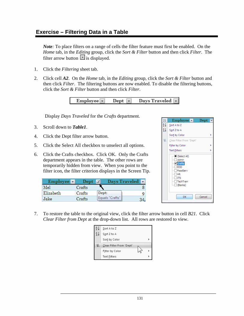
131

Exercise – Filtering Data in a Table

Note: To place filters on a range of cells the filter feature must first be enabled. On the Home tab, in the Editing group, click the Sort & Filter button and then click Filter. The filter arrow button is displayed.

1. Click the Filtering sheet tab.

2. Click cell A2. On the Home tab, in the Editing group, click the Sort & Filter button and then click Filter. The filtering buttons are now enabled. To disable the filtering buttons, click the Sort & Filter button and then click Filter.

Display Days Traveled for the Crafts department.

3. Scroll down to Table1.

4. Click the Dept filter arrow button.

5. Click the Select All checkbox to unselect all options.

6. Click the Crafts checkbox. Click OK. Only the Crafts department appears in the table. The other rows are temporarily hidden from view. When you point to the filter icon, the filter criterion displays in the Screen Tip.

7. To restore the table to the original view, click the filter arrow button in cell B21. Click Clear Filter from Dept at the drop-down list. All rows are restored to view.

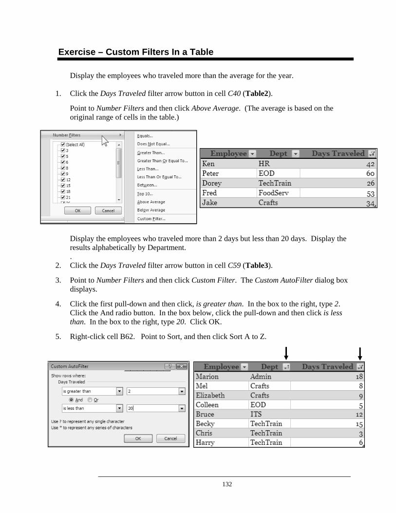
132

Exercise – Custom Filters In a Table

Display the employees who traveled more than the average for the year.

1. Click the Days Traveled filter arrow button in cell C40 (Table2).

Point to Number Filters and then click Above Average. (The average is based on the original range of cells in the table.)

Display the employees who traveled more than 2 days but less than 20 days. Display the results alphabetically by Department. .

2. Click the Days Traveled filter arrow button in cell C59 (Table3).

3. Point to Number Filters and then click Custom Filter. The Custom AutoFilter dialog box displays.

4. Click the first pull-down and then click, is greater than. In the box to the right, type 2. Click the And radio button. In the box below, click the pull-down and then click is less than. In the box to the right, type 20. Click OK.

5. Right-click cell B62. Point to Sort, and then click Sort A to Z.

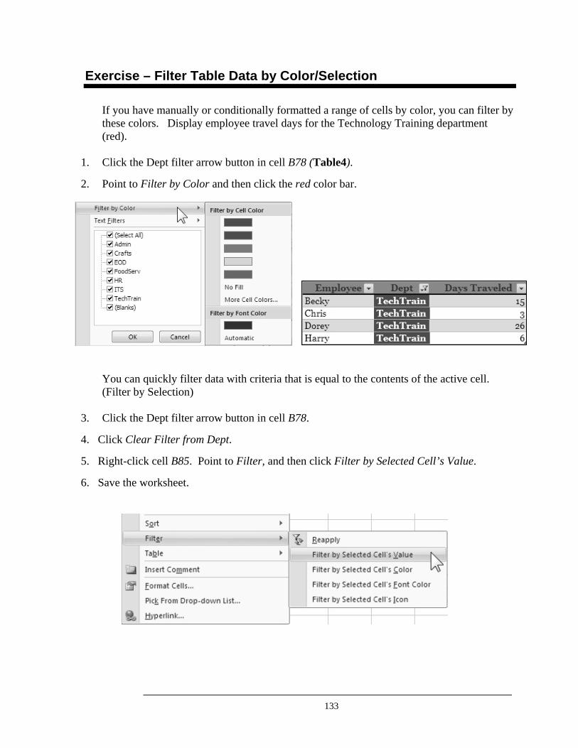
133

Exercise – Filter Table Data by Color/Selection

If you have manually or conditionally formatted a range of cells by color, you can filter by these colors. Display employee travel days for the Technology Training department (red).

1. Click the Dept filter arrow button in cell B78 (Table4).

2. Point to Filter by Color and then click the red color bar.

You can quickly filter data with criteria that is equal to the contents of the active cell. (Filter by Selection)

3. Click the Dept filter arrow button in cell B78.

4. Click Clear Filter from Dept.

5. Right-click cell B85. Point to Filter, and then click Filter by Selected Cell’s Value.


134

Charts

A chart is used to display numerical data in a graphical format allowing an easier understanding of complex data and the relationship between different sequences of data.

To create a chart in Excel 2007, numerical data on the worksheet is selected. You then plot the data by selecting a chart type located on the Insert tab, Charts group.

A chart has many elements; some displayed by default, others added as needed. You can change the display of the chart elements by moving them to other locations in the chart, resizing them, or reformatting them. Unnecessary chart elements can be removed from the chart display.

Refer to the chart on the next page and identify the following chart elements.

Chart Elements Description

Chart Area The entire area inside the Chart window, including all elements of the chart such as text, axes, titles, data points, the legend, etc.

Chart Title A specific name given to the chart

X-Axis Horizontal axis along which data categories are plotted.

Y-Axis Vertical axis along which the data values are plotted.

Axis Title Text used to label the items on the respective axis.

Data Points A bar, point, or symbol that marks a single data value; related data points makeup a chart data series.

Data Series A group of related values (data points) that share the same pattern or color.

Legend A key that identifies the data points/series.

Plot Area An area bounded by and including the two axes and all points that represent data points.

What is a Chart?

Chart Elements

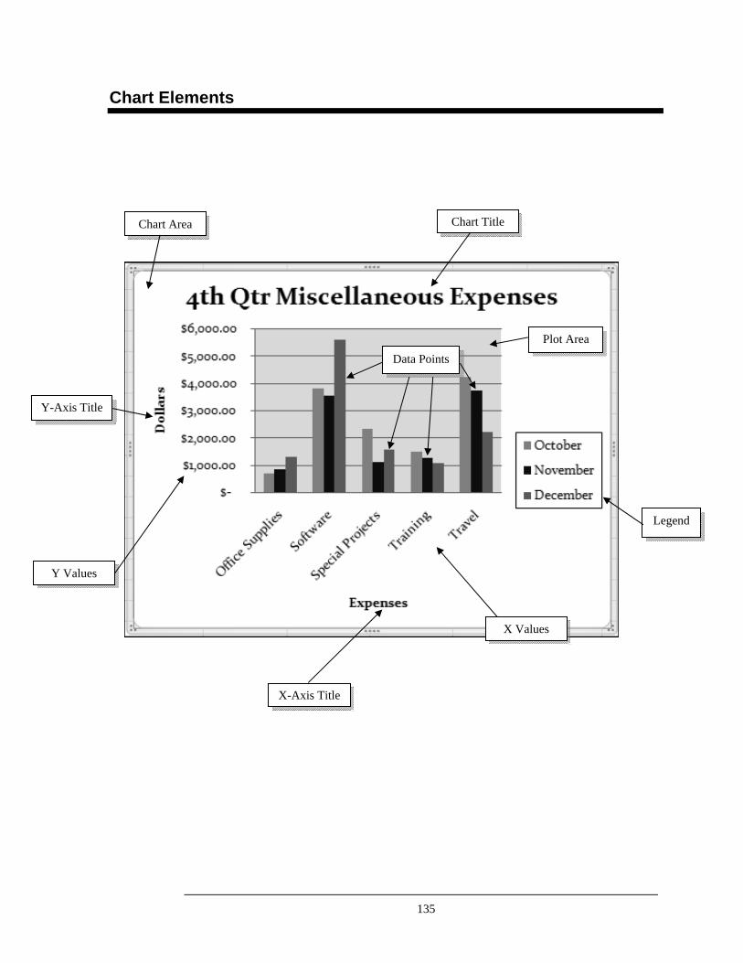
135

Chart Elements

Chart Area Chart Title

Y-Axis Title

Legend

Y Values

X-Axis Title

Plot Area Data Points

X Values

136

Chart Types

Excel has 12 chart types (including templates) from which to choose, and each chart type has a variety of formats called chart sub-types. The type of chart you select depends on how you want the data presented and what types of data you wish to emphasize. You can see a brief description and example of each chart type in Excel Help.

1. In the top right-hand corner of the screen, click the Help button.

2. In the Search text box, type Available Chart Types and then click Search.

Help Display Chart Type

Examples

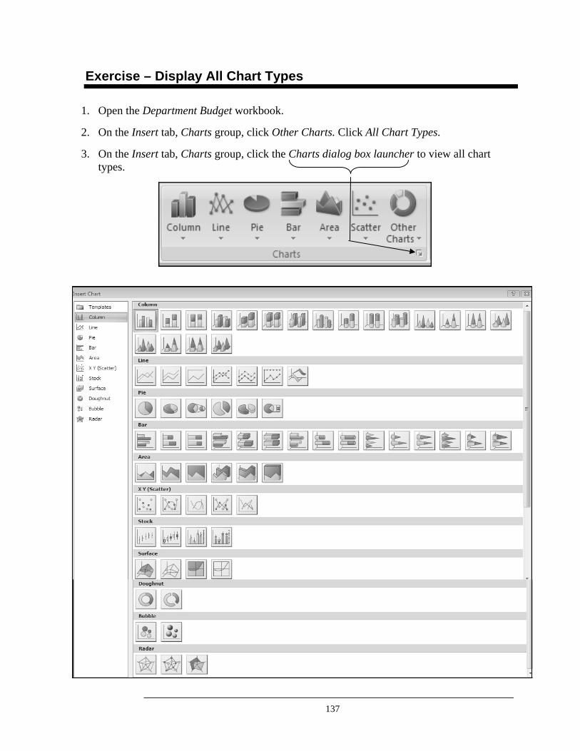
137

Exercise – Display All Chart Types

1. Open the Department Budget workbook.

2. On the Insert tab, Charts group, click Other Charts. Click All Chart Types.

3. On the Insert tab, Charts group, click the Charts dialog box launcher to view all chart types.

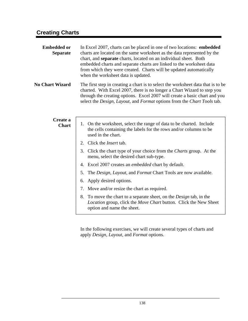
138

Creating Charts

In Excel 2007, charts can be placed in one of two locations: embedded charts are located on the same worksheet as the data represented by the chart, and separate charts, located on an individual sheet. Both embedded charts and separate charts are linked to the worksheet data from which they were created. Charts will be updated automatically when the worksheet data is updated.

The first step in creating a chart is to select the worksheet data that is to be charted. With Excel 2007, there is no longer a Chart Wizard to step you through the creating options. Excel 2007 will create a basic chart and you select the Design, Layout, and Format options from the Chart Tools tab.

1. On the worksheet, select the range of data to be charted. Include the cells containing the labels for the rows and/or columns to be used in the chart.

2. Click the Insert tab.

3. Click the chart type of your choice from the Charts group. At the menu, select the desired chart sub-type.

4. Excel 2007 creates an embedded chart by default.

5. The Design, Layout, and Format Chart Tools are now available.

6. Apply desired options.

7. Move and/or resize the chart as required.

8. To move the chart to a separate sheet, on the Design tab, in the Location group, click the Move Chart button. Click the New Sheet option and name the sheet.

In the following exercises, we will create several types of charts and apply Design, Layout, and Format options.

Embedded or Separate

No Chart Wizard

Create a Chart

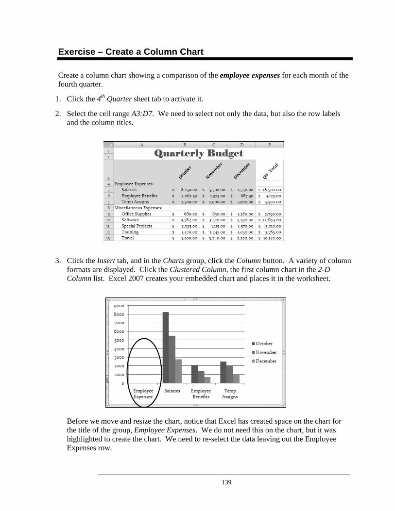
139

Exercise – Create a Column Chart

Create a column chart showing a comparison of the employee expenses for each month of the fourth quarter.

1. Click the 4th Quarter sheet tab to activate it.

2. Select the cell range A3:D7. We need to select not only the data, but also the row labels and the column titles.

3. Click the Insert tab, and in the Charts group, click the Column button. A variety of column formats are displayed. Click the Clustered Column, the first column chart in the 2-D Column list. Excel 2007 creates your embedded chart and places it in the worksheet.

Before we move and resize the chart, notice that Excel has created space on the chart for the title of the group, Employee Expenses. We do not need this on the chart, but it was highlighted to create the chart. We need to re-select the data leaving out the Employee Expenses row.

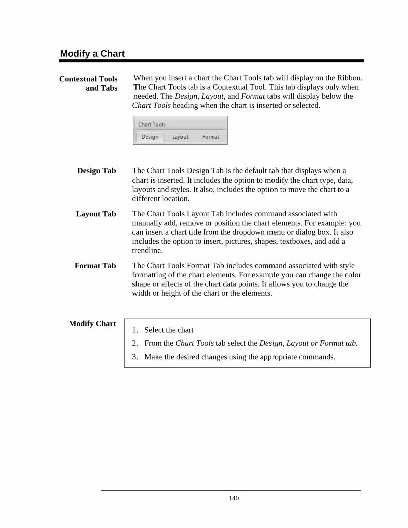
140

Modify a Chart

When you insert a chart the Chart Tools tab will display on the Ribbon. The Chart Tools tab is a Contextual Tool. This tab displays only when needed. The Design, Layout, and Format tabs will display below the Chart Tools heading when the chart is inserted or selected.

The Chart Tools Design Tab is the default tab that displays when a chart is inserted. It includes the option to modify the chart type, data, layouts and styles. It also, includes the option to move the chart to a different location.

The Chart Tools Layout Tab includes command associated with manually add, remove or position the chart elements. For example: you can insert a chart title from the dropdown menu or dialog box. It also includes the option to insert, pictures, shapes, textboxes, and add a trendline.

The Chart Tools Format Tab includes command associated with style formatting of the chart elements. For example you can change the color shape or effects of the chart data points. It allows you to change the width or height of the chart or the elements.

1. Select the chart

2. From the Chart Tools tab select the Design, Layout or Format tab.

3. Make the desired changes using the appropriate commands.

Contextual Tools and Tabs

Design Tab

Layout Tab

Format Tab

Modify Chart

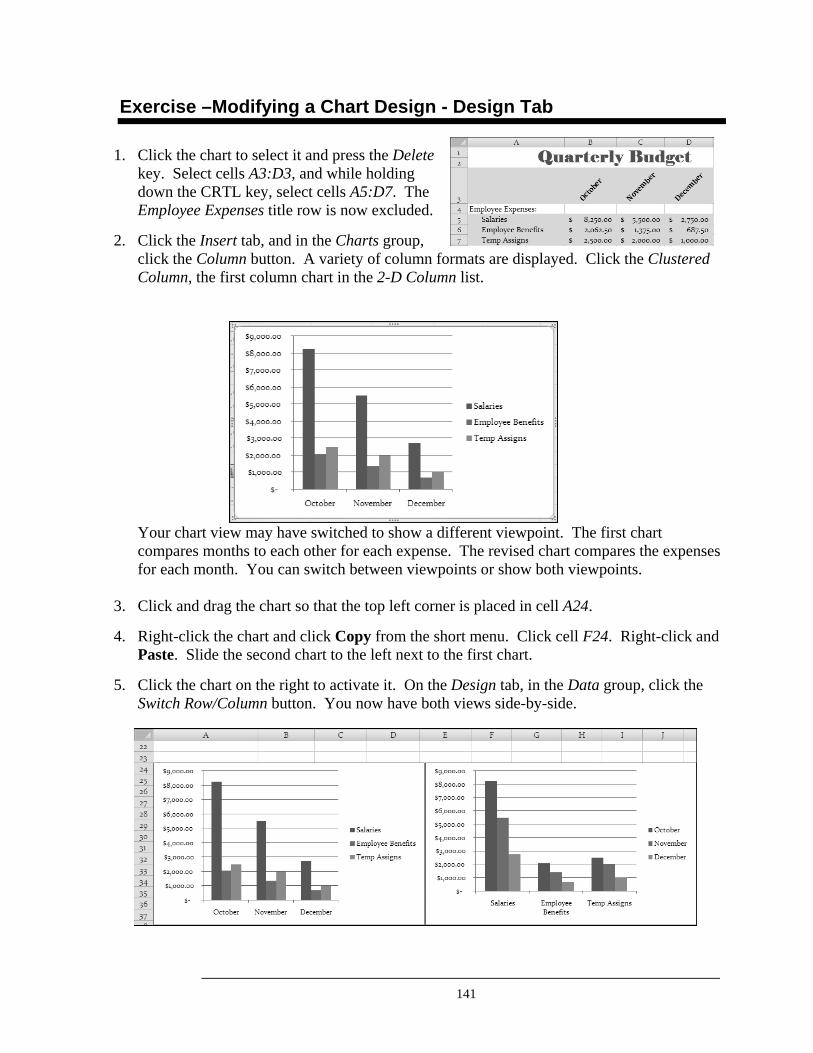
141

Exercise –Modifying a Chart Design - Design Tab

1. Click the chart to select it and press the Delete key. Select cells A3:D3, and while holding down the CRTL key, select cells A5:D7. The Employee Expenses title row is now excluded.

2. Click the Insert tab, and in the Charts group, click the Column button. A variety of column formats are displayed. Click the Clustered Column, the first column chart in the 2-D Column list.

Your chart view may have switched to show a different viewpoint. The first chart compares months to each other for each expense. The revised chart compares the expenses for each month. You can switch between viewpoints or show both viewpoints.

3. Click and drag the chart so that the top left corner is placed in cell A24.

4. Right-click the chart and click Copy from the short menu. Click cell F24. Right-click and Paste. Slide the second chart to the left next to the first chart.

5. Click the chart on the right to activate it. On the Design tab, in the Data group, click the Switch Row/Column button. You now have both views side-by-side.

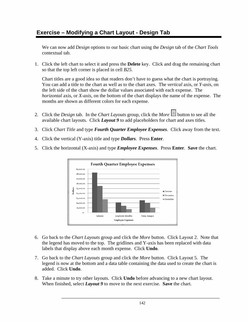
142

Exercise – Modifying a Chart Layout - Design Tab

We can now add Design options to our basic chart using the Design tab of the Chart Tools contextual tab.

1. Click the left chart to select it and press the Delete key. Click and drag the remaining chart so that the top left corner is placed in cell B25.

Chart titles are a good idea so that readers don’t have to guess what the chart is portraying. You can add a title to the chart as well as to the chart axes. The vertical axis, or Y-axis, on the left side of the chart show the dollar values associated with each expense. The horizontal axis, or X-axis, on the bottom of the chart displays the name of the expense. The months are shown as different colors for each expense.

2. Click the Design tab. In the Chart Layouts group, click the More button to see all the available chart layouts. Click Layout 9 to add placeholders for chart and axes titles.

3. Click Chart Title and type Fourth Quarter Employee Expenses. Click away from the text.

4. Click the vertical (Y-axis) title and type Dollars. Press Enter.

5. Click the horizontal (X-axis) and type Employee Expenses. Press Enter. Save the chart.

6. Go back to the Chart Layouts group and click the More button. Click Layout 2. Note that the legend has moved to the top. The gridlines and Y-axis has been replaced with data labels that display above each month expense. Click Undo.

7. Go back to the Chart Layouts group and click the More button. Click Layout 5. The legend is now at the bottom and a data table containing the data used to create the chart is added. Click Undo.

8. Take a minute to try other layouts. Click Undo before advancing to a new chart layout. When finished, select Layout 9 to move to the next exercise. Save the chart.

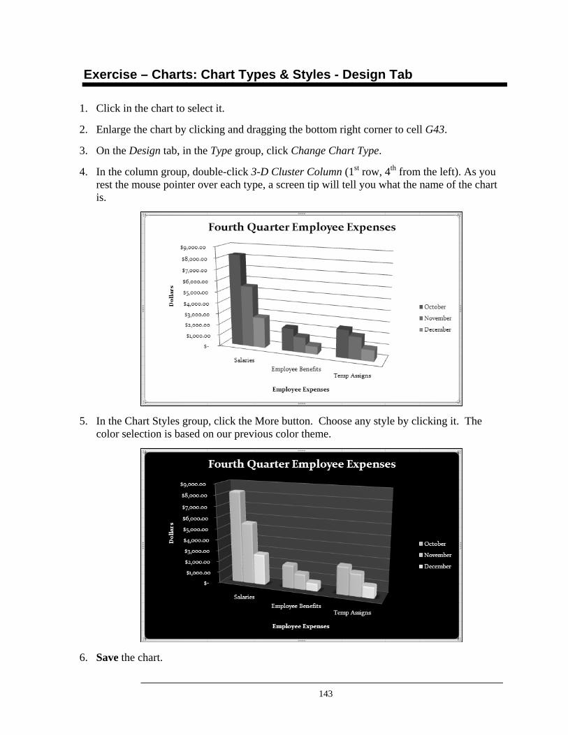
143

Exercise – Charts: Chart Types & Styles - Design Tab

1. Click in the chart to select it.

2. Enlarge the chart by clicking and dragging the bottom right corner to cell G43.

3. On the Design tab, in the Type group, click Change Chart Type.

4. In the column group, double-click 3-D Cluster Column (1st row, 4th from the left). As you rest the mouse pointer over each type, a screen tip will tell you what the name of the chart is.

5. In the Chart Styles group, click the More button. Choose any style by clicking it. The color selection is based on our previous color theme.

6. Save the chart.

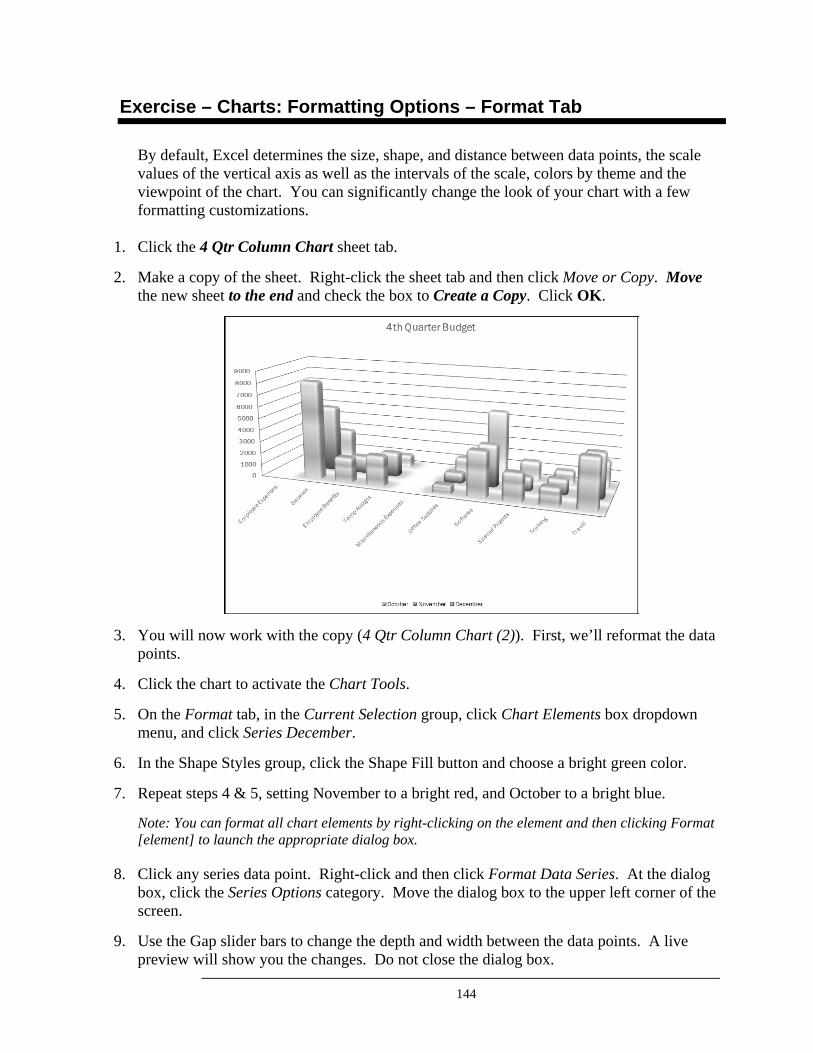
144

Exercise – Charts: Formatting Options – Format Tab

By default, Excel determines the size, shape, and distance between data points, the scale values of the vertical axis as well as the intervals of the scale, colors by theme and the viewpoint of the chart. You can significantly change the look of your chart with a few formatting customizations.

1. Click the 4 Qtr Column Chart sheet tab.

2. Make a copy of the sheet. Right-click the sheet tab and then click Move or Copy. Move the new sheet to the end and check the box to Create a Copy. Click OK.

3. You will now work with the copy (4 Qtr Column Chart (2)). First, we’ll reformat the data points.

4. Click the chart to activate the Chart Tools.

5. On the Format tab, in the Current Selection group, click Chart Elements box dropdown menu, and click Series December.

6. In the Shape Styles group, click the Shape Fill button and choose a bright green color.

7. Repeat steps 4 & 5, setting November to a bright red, and October to a bright blue.

Note: You can format all chart elements by right-clicking on the element and then clicking Format [element] to launch the appropriate dialog box.

8. Click any series data point. Right-click and then click Format Data Series. At the dialog box, click the Series Options category. Move the dialog box to the upper left corner of the screen.

9. Use the Gap slider bars to change the depth and width between the data points. A live preview will show you the changes. Do not close the dialog box.

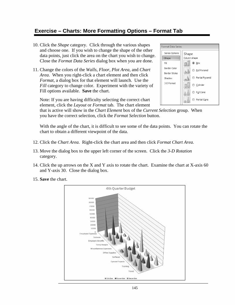
145

Exercise – Charts: More Formatting Options – Format Tab

10. Click the Shape category. Click through the various shapes and choose one. If you wish to change the shape of the other data points, just click the area on the chart you wish to change. Close the Format Data Series dialog box when you are done.

11. Change the colors of the Walls, Floor, Plot Area, and Chart Area. When you right-click a chart element and then click Format, a dialog box for that element will launch. Use the Fill category to change color. Experiment with the variety of Fill options available. Save the chart.

Note: If you are having difficulty selecting the correct chart element, click the Layout or Format tab. The chart element that is active will show in the Chart Element box of the Current Selection group. When you have the correct selection, click the Format Selection button. With the angle of the chart, it is difficult to see some of the data points. You can rotate the chart to obtain a different viewpoint of the data.

12. Click the Chart Area. Right-click the chart area and then click Format Chart Area.

13. Move the dialog box to the upper left corner of the screen. Click the 3-D Rotation category.

14. Click the up arrows on the X and Y axis to rotate the chart. Examine the chart at X-axis 60 and Y-axis 30. Close the dialog box.

15. Save the chart.

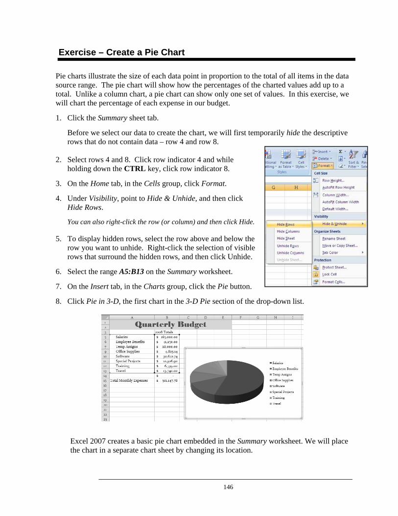
146

Exercise – Create a Pie Chart

Pie charts illustrate the size of each data point in proportion to the total of all items in the data source range. The pie chart will show how the percentages of the charted values add up to a total. Unlike a column chart, a pie chart can show only one set of values. In this exercise, we will chart the percentage of each expense in our budget.

1. Click the Summary sheet tab.

Before we select our data to create the chart, we will first temporarily hide the descriptive rows that do not contain data – row 4 and row 8.

2. Select rows 4 and 8. Click row indicator 4 and while holding down the CTRL key, click row indicator 8.

3. On the Home tab, in the Cells group, click Format.

4. Under Visibility, point to Hide & Unhide, and then click Hide Rows.

You can also right-click the row (or column) and then click Hide.

5. To display hidden rows, select the row above and below the row you want to unhide. Right-click the selection of visible rows that surround the hidden rows, and then click Unhide.

6. Select the range A5:B13 on the Summary worksheet.

7. On the Insert tab, in the Charts group, click the Pie button.

8. Click Pie in 3-D, the first chart in the 3-D Pie section of the drop-down list.

Excel 2007 creates a basic pie chart embedded in the Summary worksheet. We will place the chart in a separate chart sheet by changing its location.

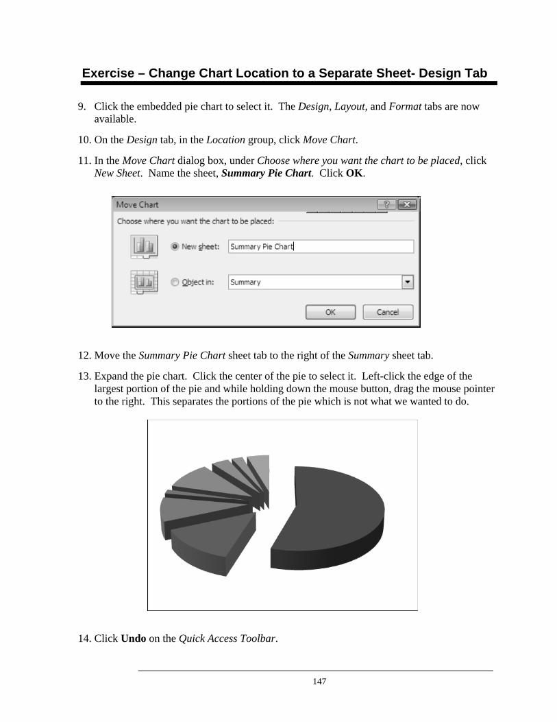
147

Exercise – Change Chart Location to a Separate Sheet- Design Tab

9. Click the embedded pie chart to select it. The Design, Layout, and Format tabs are now available.

10. On the Design tab, in the Location group, click Move Chart.

11. In the Move Chart dialog box, under Choose where you want the chart to be placed, click New Sheet. Name the sheet, Summary Pie Chart. Click OK.

12. Move the Summary Pie Chart sheet tab to the right of the Summary sheet tab.

13. Expand the pie chart. Click the center of the pie to select it. Left-click the edge of the largest portion of the pie and while holding down the mouse button, drag the mouse pointer to the right. This separates the portions of the pie which is not what we wanted to do.

14. Click Undo on the Quick Access Toolbar.

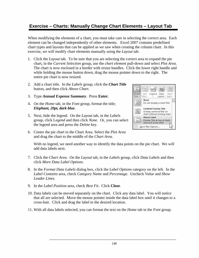
148

Exercise – Charts: Manually Change Chart Elements – Layout Tab

When modifying the elements of a chart, you must take care in selecting the correct area. Each element can be changed independently of other elements. Excel 2007 contains predefined chart types and layouts that can be applied as we saw when creating the column chart. In this exercise, we will modify chart elements manually using the Layout tab.

1. Click the Layout tab. To be sure that you are selecting the correct area to expand the pie chart, in the Current Selection group, use the chart element pull-down and select Plot Area. The chart is now enclosed in a border with resize handles. Click the lower right handle and while holding the mouse button down, drag the mouse pointer down to the right. The entire pie chart is now resized.

2. Add a chart title. In the Labels group, click the Chart Title button, and then click Above Chart.

3. Type Annual Expense Summary. Press Enter.

4. On the Home tab, in the Font group, format the title; Elephant, 20pt, dark blue.

5. Next, hide the legend. On the Layout tab, in the Labels group, click Legend and then click None. Or, you can select the legend area and press the Delete key.

6. Center the pie chart in the Chart Area. Select the Plot Area and drag the chart to the middle of the Chart Area.

With no legend, we need another way to identify the data points on the pie chart. We will add data labels next.

7. Click the Chart Area. On the Layout tab, in the Labels group, click Data Labels and then click More Data Label Options.

8. In the Format Data Labels dialog box, click the Label Options category on the left. In the Label Contains area, check Category Name and Percentage. Uncheck Value and Show Leader Lines.

9. In the Label Position area, check Best Fit. Click Close.

10. Data labels can be moved separately on the chart. Click any data label. You will notice that all are selected. Move the mouse pointer inside the data label box until it changes to a cross-hair. Click and drag the label to the desired location.

11. With all data labels selected, you can format the text on the Home tab in the Font group.

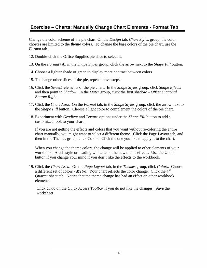
149

Exercise – Charts: Manually Change Chart Elements - Format Tab

Change the color scheme of the pie chart. On the Design tab, Chart Styles group, the color choices are limited to the theme colors. To change the base colors of the pie chart, use the Format tab.

12. Double-click the Office Supplies pie slice to select it.

13. On the Format tab, in the Shape Styles group, click the arrow next to the Shape Fill button.

14. Choose a lighter shade of green to display more contrast between colors.

15. To change other slices of the pie, repeat above steps.

16. Click the Series1 elements of the pie chart. In the Shape Styles group, click Shape Effects and then point to Shadow. In the Outer group, click the first shadow – Offset Diagonal Bottom Right.

17. Click the Chart Area. On the Format tab, in the Shape Styles group, click the arrow next to the Shape Fill button. Choose a light color to complement the colors of the pie chart.

18. Experiment with Gradient and Texture options under the Shape Fill button to add a customized look to your chart.

If you are not getting the effects and colors that you want without re-coloring the entire chart manually, you might want to select a different theme. Click the Page Layout tab, and then in the Themes group, click Colors. Click the one you like to apply it to the chart. When you change the theme colors, the change will be applied to other elements of your workbook. A cell style or heading will take on the new theme effects. Use the Undo button if you change your mind if you don’t like the effects to the workbook.

19. Click the Chart Area. On the Page Layout tab, in the Themes group, click Colors. Choose a different set of colors - Metro. Your chart reflects the color change. Click the 4th Quarter sheet tab. Notice that the theme change has had an effect on other workbook elements.

Click Undo on the Quick Access Toolbar if you do not like the changes. Save the worksheet.

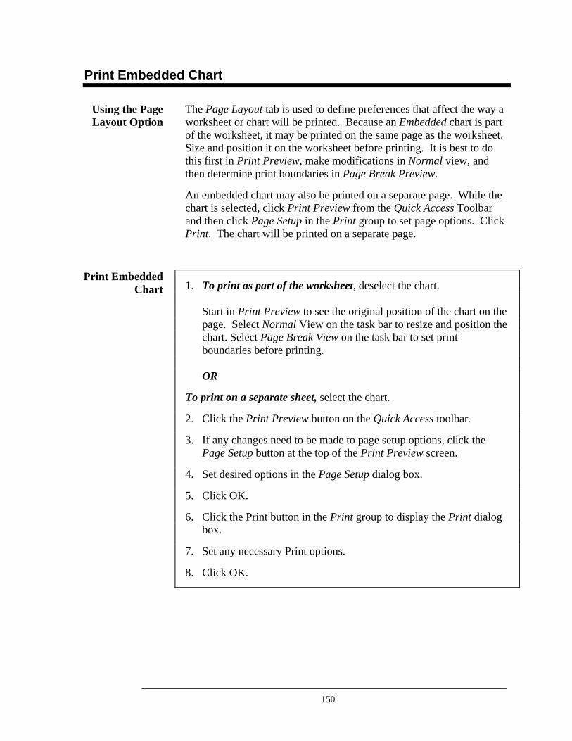
150

Print Embedded Chart

The Page Layout tab is used to define preferences that affect the way a worksheet or chart will be printed. Because an Embedded chart is part of the worksheet, it may be printed on the same page as the worksheet. Size and position it on the worksheet before printing. It is best to do this first in Print Preview, make modifications in Normal view, and then determine print boundaries in Page Break Preview.

An embedded chart may also be printed on a separate page. While the chart is selected, click Print Preview from the Quick Access Toolbar and then click Page Setup in the Print group to set page options. Click Print. The chart will be printed on a separate page.

1. To print as part of the worksheet, deselect the chart. Start in Print Preview to see the original position of the chart on the page. Select Normal View on the task bar to resize and position the chart. Select Page Break View on the task bar to set print boundaries before printing. OR

To print on a separate sheet, select the chart.

2. Click the Print Preview button on the Quick Access toolbar.

3. If any changes need to be made to page setup options, click the Page Setup button at the top of the Print Preview screen.

4. Set desired options in the Page Setup dialog box.

5. Click OK.

6. Click the Print button in the Print group to display the Print dialog box.

7. Set any necessary Print options.

8. Click OK.

Using the Page Layout Option

Print Embedded Chart

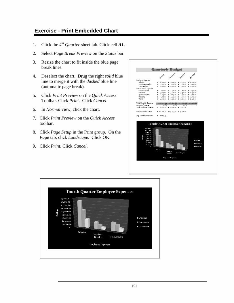
151

Exercise - Print Embedded Chart

1. Click the 4th Quarter sheet tab. Click cell A1.

2. Select Page Break Preview on the Status bar.

3. Resize the chart to fit inside the blue page break lines.

4. Deselect the chart. Drug the right solid blue line to merge it with the dashed blue line (automatic page break).

5. Click Print Preview on the Quick Access Toolbar. Click Print. Click Cancel.

6. In Normal view, click the chart.

7. Click Print Preview on the Quick Access toolbar.

8. Click Page Setup in the Print group. On the Page tab, click Landscape. Click OK.

9. Click Print. Click Cancel.

152

Print Separate Chart Sheet

Page Setup options for a separate chart sheet may be set independently from the page setup options for the worksheet containing the data plotted in the chart. By default a separate chart sheet will print in the landscape orientation filling the entire page.

Once Page Setup options have been set for the chart page, use the Print button in the Print group, Print Preview to print the chart.


2. If any changes need to be made to Page Setup options, click the Page Setup button in the Print group.

3. Set any desired Page Setup options.

4. Click OK.

5. Click the Print button in the Print group to display the Print dialog box.

6. Set any necessary Print options.

7. Click OK.

Page Setup Options

Print a Separate Chart Sheet

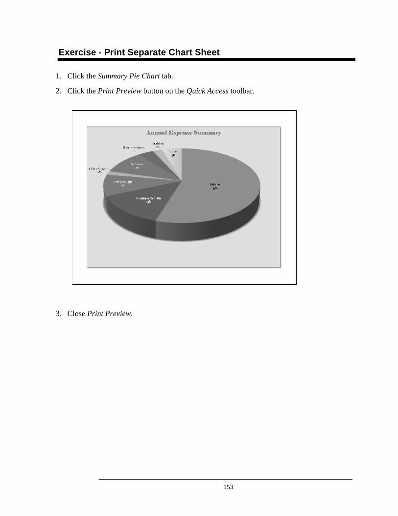
153

Exercise - Print Separate Chart Sheet

1. Click the Summary Pie Chart tab.


3. Close Print Preview.

154

Integrating Programs – Paste & Paste Special (Link/Embed/Picture)

Microsoft Office allows you to easily exchange data from one program to another. There are 2 main ways in which to integrate information between the programs: Paste and Paste Special Each MS Office program has its unique Paste Special options, but the following three options are common to all of them: Linking, Embedding, and Pasting as a Picture.

Which is the best method? It depends on your need. Each method has its pros and cons – depending on how you see it!

When you copy/ paste data between programs, the source of the data operates independently from the data’s destination. In other words, if you copied data from Word to Excel and updated the data in the Word document, the update is not reflected in the Excel spreadsheet. You would need to copy and paste the data each time a change in the source document occurred.

When data is linked, the data exists in the source program, but not as independent data in the destination program. The destination contains only a code that identifies the location of the source; it is like having a hyperlink. Since data is located only in the source program, changes made to the source data is reflected in the destination program. Links are automatically updated when the destination program is opened. Or you can update it any time by right clicking the linked object and selecting Update Link option. This is useful when: • You want your presentation automatically updated when you

change the data or charts in the Excel worksheet.

An object can be embedded in a destination program. An embedded object resides in the source program as well as the destination program. Any changes made to the source object are not reflected in the destination object. The advantage to embedding is that you can edit an embedded object in the destination program using the tools of the source program. This is useful for example, when: • You want the PowerPoint presentation to be a self-contained

package that includes your entire Excel workbook. • You want to be sure that anyone who opens your presentation can see

and edit the Excel data that is associated with the embedded object. An object can be pasted in a destination program as a Picture. For example, you can paste the Excel chart into your PowerPoint presentation as a static Microsoft Office Graphic Object. The chart is now treated as any other graphic. This is useful when: • You don’t need to format the chart or update the chart data.

Let’s Exchange Information

Best Way?

Paste Data

Link the Data

Embed the Data

Paste Data as a Picture

155

Exercise – Copy & Paste a Word Table To Excel

After creating a table in a Word document, you may realize that you would like to perform some calculations on your data. In this case to avoid mistakes or duplicating data entry, it would be best to copy and paste your Word table into the Excel program, and then create any appropriate formulas to calculate or summarize your data. After all calculations are done you can paste the table back into your word document.

1. Open the Department Budget Charts Excel file located on the Desktop in the Excel 07 Class folder.

2. Click the Integrate sheet tab to activate it.

3. Open the TechnologyHours Word document located on the Desktop in the Excel 07 Class folder.

4. Copy the Word table.

5. Click the Department Budget Charts.xlsx button on the task bar.

6. Select cell A1.

7. Click Paste button on the Home tab in the Clipboard group to paste the Word table. Although the object is a table in Word, it does not copy as a table into Excel and therefore, does not have table capabilities.

8. Now you can format this data as an Excel table, and insert any necessary formulas to perform your calculations.


10. Close the Technology Hours document.

156

Exercise – Link an Excel Chart to PowerPoint Presentation

A chart is a much better way of conveying numerical information than a slide filled with numbers! Linking allows you to copy a chart created in excel and paste it into a PowerPoint presentation. Your linked chart will automatically update when you change the data or chart in Excel worksheet, paste chart into the Power Point as a link.

1. Open the Department Budget Presentation PowerPoint file located on the Desktop in the Excel 07 Class folder.


3. Click the Link Chart sheet tab.

4. Select the chart.

5. On the Home tab in the Clipboard group, click Copy button to copy the chart.

6. Click the Department Budget Presentation.pptx button on the task bar.

7. Select the second slide.

8. On the Home tab in the Clipboard group, click the Paste button.

• The chart is inserted with a Paste Special icon in the lower-right corner.

9. Click the Paste Special icon.

10. The Chart (linked to Excel data) and the Use Destination Theme is selected by default.

• Leave these choices if you would like your chart being linked to the Excel data, or select any other method in which you would like your chart inserted.

11. Save your presentation.

157

Exercise – Updating Linked Data

12. Go back to the Department Budget Charts workbook. The Link Chart sheet is active.

13. Click cell D5. Type 20,000.00, press Enter.

14. Click cell D7. Type 1,000.00, press Enter.

Each time when you pressed enter after making changes to the data, the corresponding data points in the linked chart have been automatically updated to reflect the changes.

15. Save and Close the presentation.

16. Click cell C7. Type 4,000.00, press Enter.


18. Open the Department Budget Presentation.

19. Select the slide that contains the chart. Notice that the data does not reflect the change made in the source workbook.

20. Select the chart.

21. Click the Refresh Data button on the Chart Tools Design contextual tab, in the Data group to refresh the data. The chart now reflects the changes.

Note:

• In contrast, when you are working with linked Excel data in Word, the data will automatically update each time you open the document. The following dialog box will display, and you will need to decide if you would like to update the data in your document or not.

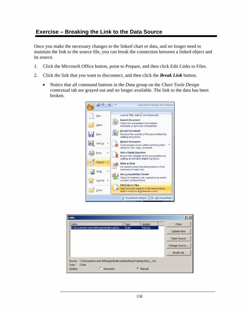
158

Exercise – Breaking the Link to the Data Source

Once you make the necessary changes to the linked chart or data, and no longer need to maintain the link to the source file, you can break the connection between a linked object and its source.

1. Click the Microsoft Office button, point to Prepare, and then click Edit Links to Files.

2. Click the link that you want to disconnect, and then click the Break Link button.

• Notice that all command buttons in the Data group on the Chart Tools Design contextual tab are grayed out and no longer available. The link to the data has been broken.

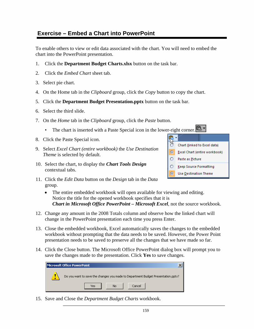
159

Exercise – Embed a Chart into PowerPoint

To enable others to view or edit data associated with the chart. You will need to embed the chart into the PowerPoint presentation.


2. Click the Embed Chart sheet tab.

3. Select pie chart.

4. On the Home tab in the Clipboard group, click the Copy button to copy the chart.

5. Click the Department Budget Presentation.pptx button on the task bar.

6. Select the third slide.

7. On the Home tab in the Clipboard group, click the Paste button.

• The chart is inserted with a Paste Special icon in the lower-right corner.

8. Click the Paste Special icon.

9. Select Excel Chart (entire workbook) the Use Destination Theme is selected by default.

10. Select the chart, to display the Chart Tools Design contextual tabs.

11. Click the Edit Data button on the Design tab in the Data group. • The entire embedded workbook will open available for viewing and editing.

Notice the title for the opened workbook specifies that it is Chart in Microsoft Office PowerPoint – Microsoft Excel, not the source workbook.

12. Change any amount in the 2008 Totals column and observe how the linked chart will change in the PowerPoint presentation each time you press Enter.

13. Close the embedded workbook, Excel automatically saves the changes to the embedded workbook without prompting that the data needs to be saved. However, the Power Point presentation needs to be saved to preserve all the changes that we have made so far.

14. Click the Close button. The Microsoft Office PowerPoint dialog box will prompt you to save the changes made to the presentation. Click Yes to save changes.

15. Save and Close the Department Budget Charts workbook.

160

Notes

161

Appendices

Additional Features in Excel 2007

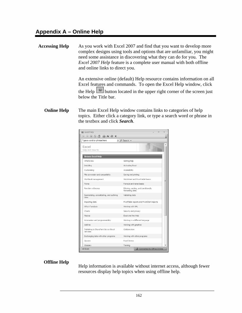
162

Appendix A – Online Help

As you work with Excel 2007 and find that you want to develop more complex designs using tools and options that are unfamiliar, you might need some assistance in discovering what they can do for you. The Excel 2007 Help feature is a complete user manual with both offline and online links to direct you. An extensive online (default) Help resource contains information on all Excel features and commands. To open the Excel Help window, click the Help button located in the upper right corner of the screen just below the Title bar.

The main Excel Help window contains links to categories of help topics. Either click a category link, or type a search word or phrase in the textbox and click Search.

Help information is available without internet access, although fewer resources display help topics when using offline help.

Accessing Help

Online Help

Offline Help

163

Appendix B – Smart Tags

Use Smart Tags to quickly perform a useful task. The type of Smart Tag you see depends on the action you are performing. Smart Tags display as purple triangles in the upper-left corner of a cell, or they can also display as a button with a drop-down arrow next to a cell. Smart Tags display when you perform an action on the spreadsheet that Excel wants to help you with. The Smart Tag will provide some helpful options to you. To use a Smart Tag in Excel, you must first perform an action that will display a Smart Tag. The types of Smart Tags and the functions they perform are listed below:

The AutoCorrect Options button first appears as a small, blue box when you rest the mouse pointer near text that was automatically corrected, and changes to a button icon when you point to it. If you find on occasion that you don't want text to be corrected, you can undo a correction or turn AutoCorrect options on or off by clicking the button and making a selection.

The Paste Options button appears just below your pasted selection after you paste text or data. When you click the button, a list appears that lets you determine how the information is pasted into your worksheet. The available options depend on the type of content you are pasting, the program you are pasting from, and the format of the text where you are pasting.

The Auto Fill Options button appears just below your filled selection after you fill text or data in a worksheet. When you click the button, a list appears to give you options for how to fill the text or data. The available options depend on the content you are filling, the program you are filling from, and the format of the text or data you are filling.

The Trace Error button appears next to the cell in which a formula error occurs, and a green triangle appears in the upper-left of the cell. When you click the arrow next to Trace Error, a list appears to give you options for error checking.

The Insert Options button appears next to your inserted cells, rows, or columns. When you click the arrow next to Insert Options, a list of formatting options appears

Save Time

How Do They Work?

AutoCorrect Options

Paste Options

AutoFill Options

Trace Error

Insert Options

164

Appendix C – Locking Specific Cells

When you share a workbook, you may want to protect data in specific workbook cells to prevent it from being accidentally or deliberately changed, moved, or deleted. You can also prevent users from changing the structure of a worksheet. A password can be used to allow users access. Protection can be removed as necessary.

By default, when you protect a worksheet, all cells are locked and no changes can be made to a locked cell. Before protecting the sheet, unlock the cells that can be modified. Adding a password to unlock cells is optional and is only intended to allow access to certain users while helping to prevent changes by others. This level of password protection does not guarantee security for sensitive data; secure the workbook itself with a password for optimal security.

1. Select the worksheet you want to protect.

2. Select any cells or ranges that you want to unlock (allow changes). On the Home tab, in the Cells group, click Format, and then click Format Cells. On the Protection tab, clear the Locked check box, and then click OK.

3. To hide formulas you do not want visible, select the cells you want to hide. On the Home tab, in the Cells group, click Format, and then click Format Cells. On the Protection tab, select the Hidden check box, and then click OK.

4. To protect the worksheet, on the Review tab, in the Changes group, click Protect Sheet. In the Protect Sheet dialog box in the Allow all users of this worksheet to list, select the actions that you want users to be able to perform. In the Password to unprotect sheet box, type a password for the sheet, click OK, and then retype the password to confirm it. (If you do not supply a password, any user can unprotect the sheet and make changes. Don’t forget your password!)

5. To remove protection from a worksheet, on the Review tab, in the Changes group, click Unprotect Sheet. Type the password if prompted.

Protect Formulas from being

changed

Passwords are Optional

Steps to Protect Worksheet

Elements

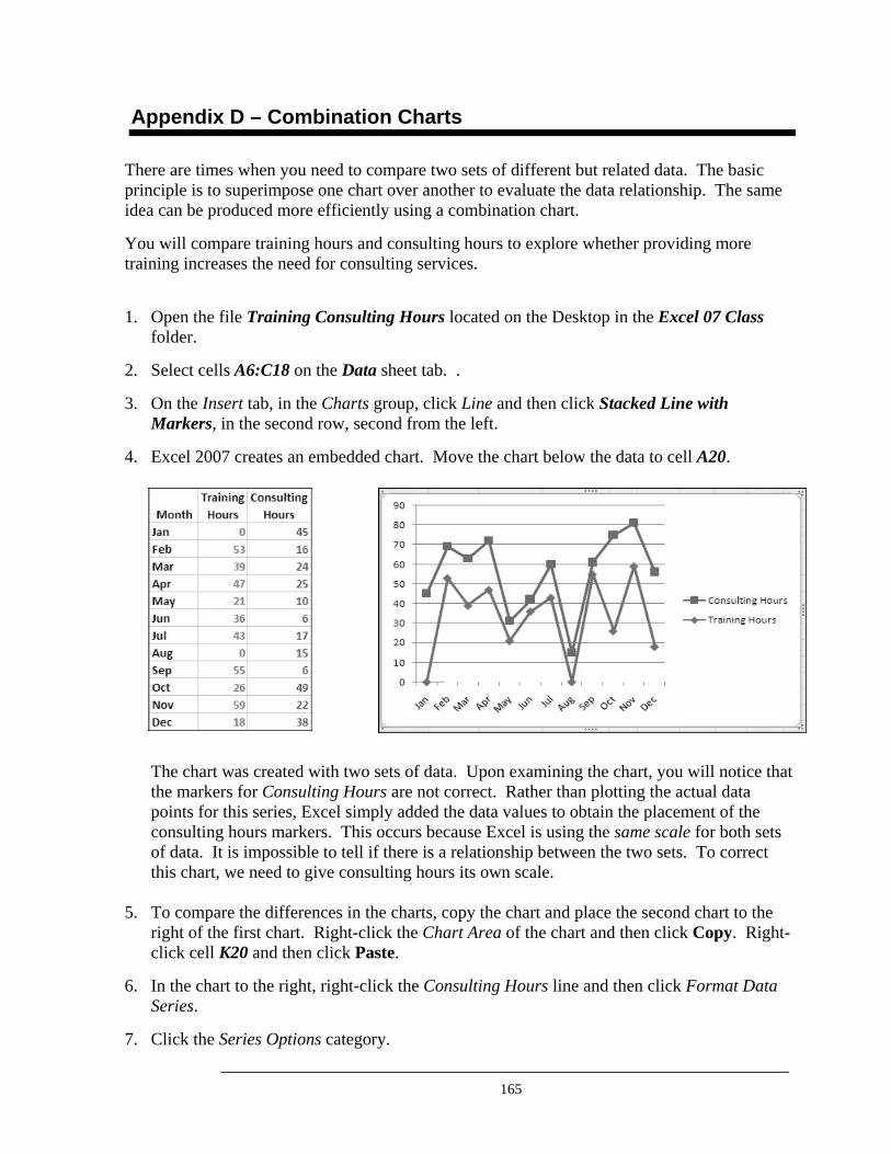
165

Appendix D – Combination Charts

There are times when you need to compare two sets of different but related data. The basic principle is to superimpose one chart over another to evaluate the data relationship. The same idea can be produced more efficiently using a combination chart.

You will compare training hours and consulting hours to explore whether providing more training increases the need for consulting services.

1. Open the file Training Consulting Hours located on the Desktop in the Excel 07 Class

folder.

2. Select cells A6:C18 on the Data sheet tab. .

3. On the Insert tab, in the Charts group, click Line and then click Stacked Line with Markers, in the second row, second from the left.

4. Excel 2007 creates an embedded chart. Move the chart below the data to cell A20.

The chart was created with two sets of data. Upon examining the chart, you will notice that the markers for Consulting Hours are not correct. Rather than plotting the actual data points for this series, Excel simply added the data values to obtain the placement of the consulting hours markers. This occurs because Excel is using the same scale for both sets of data. It is impossible to tell if there is a relationship between the two sets. To correct this chart, we need to give consulting hours its own scale.

5. To compare the differences in the charts, copy the chart and place the second chart to the right of the first chart. Right-click the Chart Area of the chart and then click Copy. Right-click cell K20 and then click Paste.

6. In the chart to the right, right-click the Consulting Hours line and then click Format Data Series.

7. Click the Series Options category.

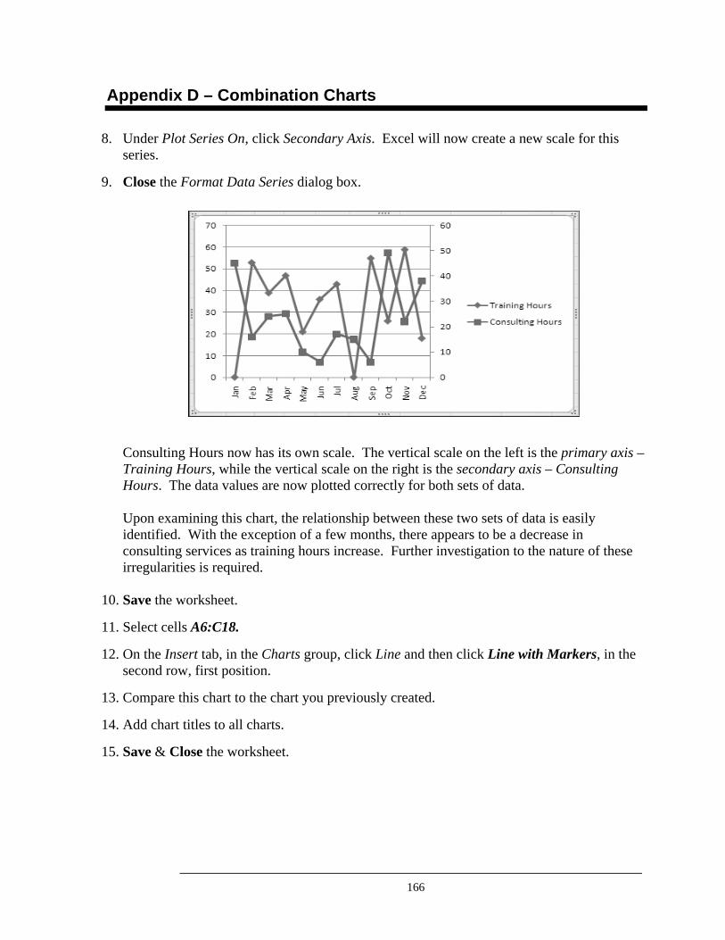
166

Appendix D – Combination Charts

8. Under Plot Series On, click Secondary Axis. Excel will now create a new scale for this series.

9. Close the Format Data Series dialog box.

Consulting Hours now has its own scale. The vertical scale on the left is the primary axis – Training Hours, while the vertical scale on the right is the secondary axis – Consulting Hours. The data values are now plotted correctly for both sets of data. Upon examining this chart, the relationship between these two sets of data is easily identified. With the exception of a few months, there appears to be a decrease in consulting services as training hours increase. Further investigation to the nature of these irregularities is required.


11. Select cells A6:C18.

12. On the Insert tab, in the Charts group, click Line and then click Line with Markers, in the second row, first position.

13. Compare this chart to the chart you previously created.

14. Add chart titles to all charts.

15. Save & Close the worksheet.

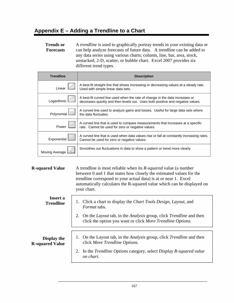
167

Appendix E – Adding a Trendline to a Chart

A trendline is used to graphically portray trends in your existing data or can help analyze forecasts of future data. A trendline can be added to any data series using various charts; column, line, bar, area, stock, unstacked, 2-D, scatter, or bubble chart. Excel 2007 provides six different trend types.

Trendline Description

Linear A best-fit straight line that shows increasing or decreasing values at a steady rate. Used with simple linear data sets.

Logarithmic A best-fit curved line used when the rate of change in the data increases or decreases quickly and then levels out. Uses both positive and negative values.

Polynomial A curved line used to analyze gains and losses. Useful for large data sets where the data fluctuates.

Power A curved line that is used to compare measurements that increases at a specific rate. Cannot be used for zero or negative values.

Exponential A curved line that is used when data values rise or fall at constantly increasing rates. Cannot be used for zero or negative values.

Moving Average Smoothes out fluctuations in data to show a pattern or trend more clearly.

A trendline is most reliable when its R-squared value (a number between 0 and 1 that states how closely the estimated values for the trendline correspond to your actual data) is at or near 1. Excel automatically calculates the R-squared value which can be displayed on your chart.

1. Click a chart to display the Chart Tools Design, Layout, and Format tabs.

2. On the Layout tab, in the Analysis group, click Trendline and then click the option you want or click More Trendline Options.

1. On the Layout tab, in the Analysis group, click Trendline and then click More Trendline Options.

2. In the Trendline Options category, select Display R-squared value on chart.

Trends or Forecasts

R-squared Value

Insert a Trendline

Display the R-squared Value

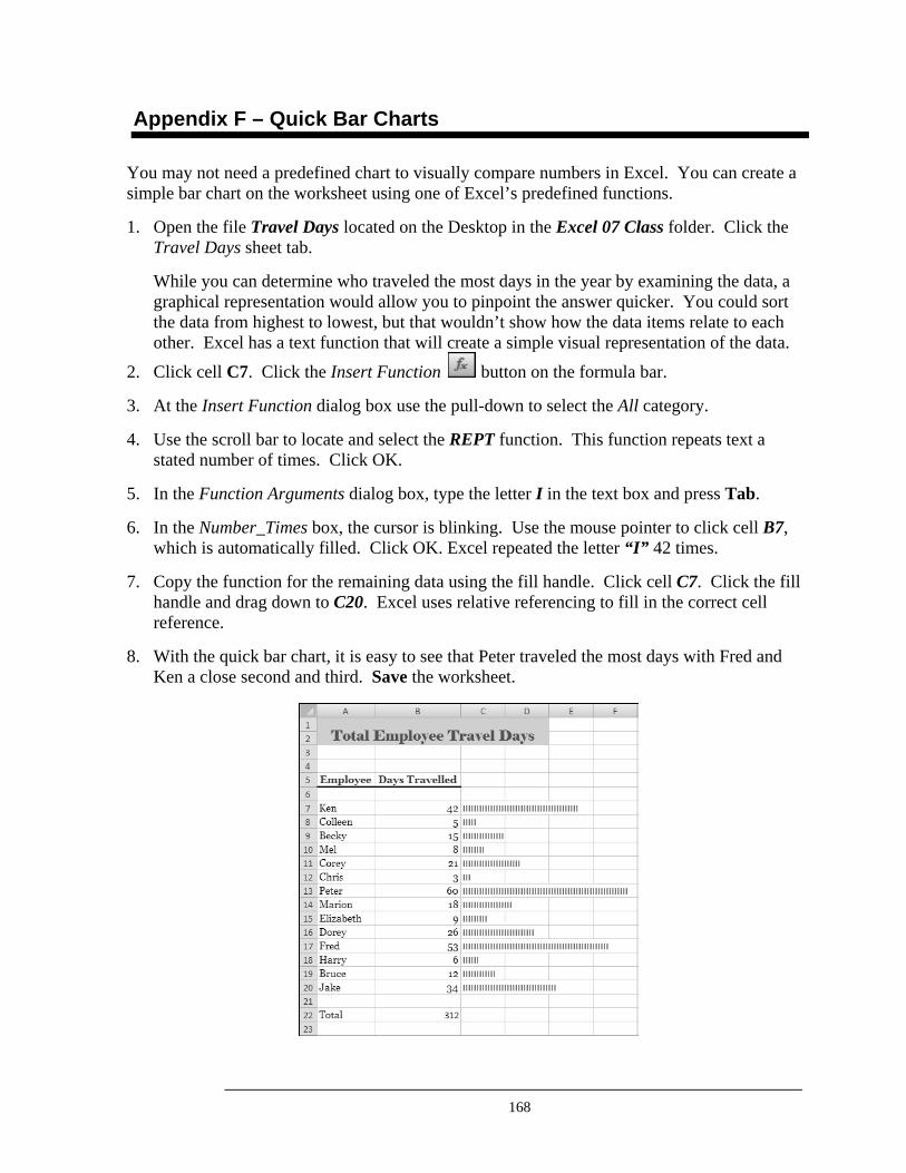
168

Appendix F – Quick Bar Charts

You may not need a predefined chart to visually compare numbers in Excel. You can create a simple bar chart on the worksheet using one of Excel’s predefined functions.

1. Open the file Travel Days located on the Desktop in the Excel 07 Class folder. Click the Travel Days sheet tab.

While you can determine who traveled the most days in the year by examining the data, a graphical representation would allow you to pinpoint the answer quicker. You could sort the data from highest to lowest, but that wouldn’t show how the data items relate to each other. Excel has a text function that will create a simple visual representation of the data.

2. Click cell C7. Click the Insert Function button on the formula bar.

3. At the Insert Function dialog box use the pull-down to select the All category.

4. Use the scroll bar to locate and select the REPT function. This function repeats text a stated number of times. Click OK.

5. In the Function Arguments dialog box, type the letter I in the text box and press Tab.

6. In the Number_Times box, the cursor is blinking. Use the mouse pointer to click cell B7, which is automatically filled. Click OK. Excel repeated the letter “I” 42 times.

7. Copy the function for the remaining data using the fill handle. Click cell C7. Click the fill handle and drag down to C20. Excel uses relative referencing to fill in the correct cell reference.

8. With the quick bar chart, it is easy to see that Peter traveled the most days with Fred and Ken a close second and third. Save the worksheet.

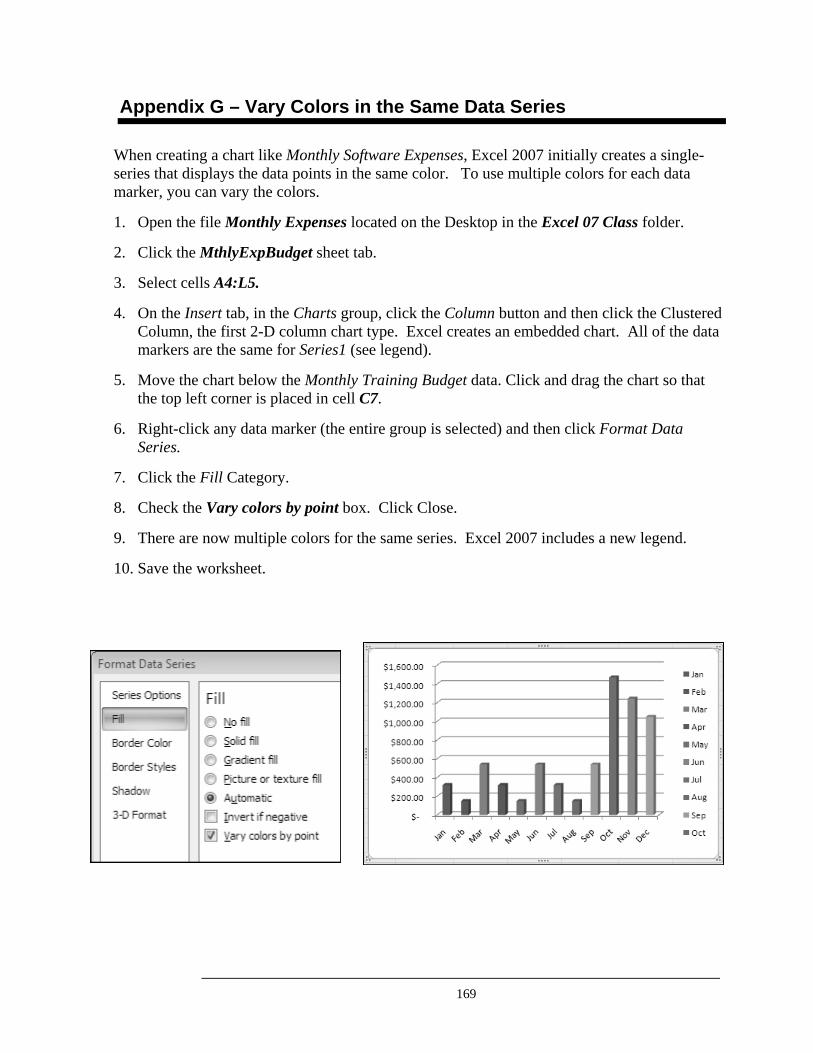
169

Appendix G – Vary Colors in the Same Data Series

When creating a chart like Monthly Software Expenses, Excel 2007 initially creates a single-series that displays the data points in the same color. To use multiple colors for each data marker, you can vary the colors.

1. Open the file Monthly Expenses located on the Desktop in the Excel 07 Class folder.

2. Click the MthlyExpBudget sheet tab.

3. Select cells A4:L5.

4. On the Insert tab, in the Charts group, click the Column button and then click the Clustered Column, the first 2-D column chart type. Excel creates an embedded chart. All of the data markers are the same for Series1 (see legend).

5. Move the chart below the Monthly Training Budget data. Click and drag the chart so that the top left corner is placed in cell C7.

6. Right-click any data marker (the entire group is selected) and then click Format Data Series.

7. Click the Fill Category.

8. Check the Vary colors by point box. Click Close.

9. There are now multiple colors for the same series. Excel 2007 includes a new legend.


170

Appendix H – Picture Charts

You can make your charts more interesting by adding images to various chart elements.

1. Open the file Monthly Expenses located on the Desktop in the Excel 07 Class folder.


3. On the Insert tab, in the Charts group, click the Column button and then click the first 3-D column chart type. Excel creates an embedded chart.

4. Move the chart below the Monthly Software Budget data. Click and drag the chart so that the top left corner is placed in cell C30.

5. Click cell G28. Change the data to 1850 and then press Enter. The column for the July software expense is updated and the chart immediately shows the change as the data point for July is taller.

6. Relocate the chart to a new worksheet. Click the chart to select it. On the Design tab in the Location group, click the Move Chart button.

7. At the Move Chart dialog box, click New Sheet and name the sheet SoftwareExpChart. Click OK.

8. Delete the legend.

9. Add a chart title. On the Layout tab, in the Labels group, click the Chart Title button and then click Above Chart.

10. Type Monthly Software Expenses and then press Enter.

11. Delete the gridlines. Click the gridline and press the Delete Key.

12. Delete the vertical axis values.

13. Add Data Labels to show the values of the data points. On the Layout tab, in the Labels group, click the Data Labels button and then click Show.

14. To add an image to the background plot area, select the Plot Area. Make sure you have the correct area by clicking the Layout tab, Current Selection group, Chart Elements box.

15. Right-click on the border surrounding the Plot Area and then click Format Plot Area. A dialog box opens.

16. In the Fill category, click Picture or texture fill. More options become available to you.

17. Under Insert from, click the File button. Navigate to the Desktop and double-click the Excel 07 Class folder. Double-click the Clips folder.

18. Click dollar sign.jpg and then Insert.

19. Slide the transparency rule to 80%. Click Close.

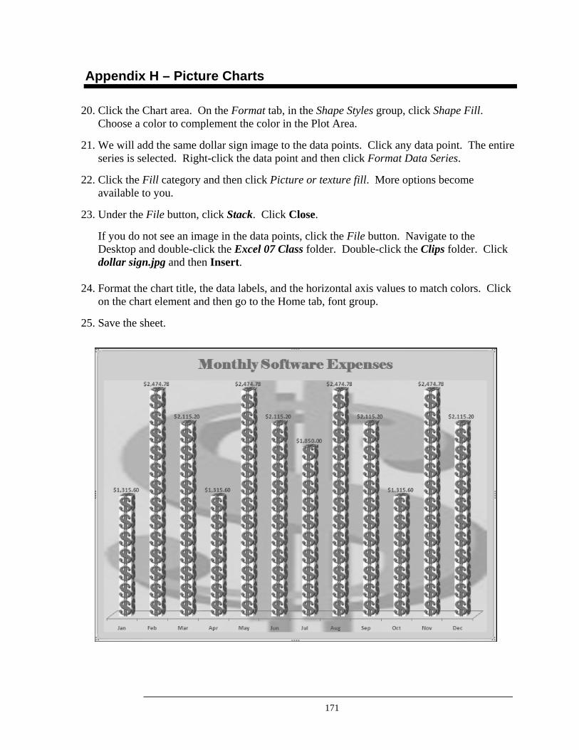
171

Appendix H – Picture Charts

20. Click the Chart area. On the Format tab, in the Shape Styles group, click Shape Fill. Choose a color to complement the color in the Plot Area.

21. We will add the same dollar sign image to the data points. Click any data point. The entire series is selected. Right-click the data point and then click Format Data Series.

22. Click the Fill category and then click Picture or texture fill. More options become available to you.

23. Under the File button, click Stack. Click Close.

If you do not see an image in the data points, click the File button. Navigate to the Desktop and double-click the Excel 07 Class folder. Double-click the Clips folder. Click dollar sign.jpg and then Insert.

24. Format the chart title, the data labels, and the horizontal axis values to match colors. Click on the chart element and then go to the Home tab, font group.

25. Save the sheet.

172

Appendix I – Creating Chart Templates

If you want to reuse a chart that you customized for your needs, you can save that chart as a template. The template will be stored in the chart templates folder (.crtx).

Once the template is stored in the charts folder, it can be used in other workbooks as any other predefined chart type. The template becomes available under Templates in both the Insert Chart dialog box (Insert tab, Charts group, dialog box launcher) and the Change Chart Type dialog box (Design tab, Type group, Change Chart Type).

1. Click the chart you want to save as a template.

2. On the Design tab, in the Type group, click Save as Template.

3. Name the template.

4. Click Save.

Customizable

Reuse in all workbooks

Steps to save a template

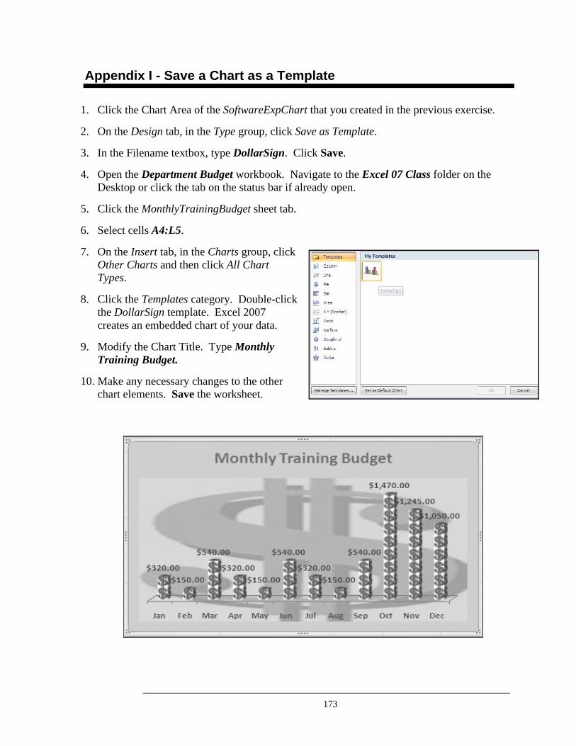
173

Appendix I - Save a Chart as a Template

1. Click the Chart Area of the SoftwareExpChart that you created in the previous exercise.

2. On the Design tab, in the Type group, click Save as Template.

3. In the Filename textbox, type DollarSign. Click Save.

4. Open the Department Budget workbook. Navigate to the Excel 07 Class folder on the Desktop or click the tab on the status bar if already open.

5. Click the MonthlyTrainingBudget sheet tab.


7. On the Insert tab, in the Charts group, click Other Charts and then click All Chart Types.

8. Click the Templates category. Double-click the DollarSign template. Excel 2007 creates an embedded chart of your data.

9. Modify the Chart Title. Type Monthly Training Budget.

10. Make any necessary changes to the other chart elements. Save the worksheet.

174

Appendix J - Formula Names

Your formulas will be much easier to understand and maintain by using names. You can define a name for a cell range, function, constant, or table. Names can be easily updated, audited, and managed.

For example, in our Department Budget worksheet, we calculated the Total Monthly Expenses for January as: =B2+B3+B4+B5+B6+B7+B8+B9. We can improve on the clarity and understanding of this formula by naming the cell range as JanuaryExpenses. Our formula becomes much more understandable as we can now state the formula as =SUM(JanuaryExpenses).

Names can be specific to either a specific worksheet or to an entire workbook. The location within which the name is recognized without qualification is its scope. All names must be unique within its scope.

By default, names use absolute cell references.

There are three ways to define a name:

Define a name by: Description

Name box on the formula bar Best used for creating a workbook level name for a selected range.

Created from selection Use existing row and column labels by using a selection of cells in the worksheet.

New name dialog box Best used for more flexibility in creating names for local worksheet level or creating a name comment.

The first character of a name must be a letter, an underscore character (_) or a backslash (\). Remaining characters can be letters, numbers, periods, and underscore characters. Spaces are not allowed as part of a name. A name can contain up to 255 characters. Excel does not distinguish between uppercase and lowercase characters in names.

Formulas more Understandable

Scope of a Name

Syntax Rules

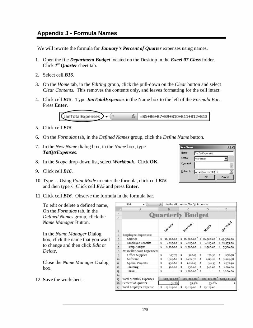
175

Appendix J - Formula Names

We will rewrite the formula for January’s Percent of Quarter expenses using names.

1. Open the file Department Budget located on the Desktop in the Excel 07 Class folder. Click 1st Quarter sheet tab.

2. Select cell B16.

3. On the Home tab, in the Editing group, click the pull-down on the Clear button and select Clear Contents. This removes the contents only, and leaves formatting for the cell intact.

4. Click cell B15. Type JanTotalExpenses in the Name box to the left of the Formula Bar. Press Enter.

5. Click cell E15.

6. On the Formulas tab, in the Defined Names group, click the Define Name button.

7. In the New Name dialog box, in the Name box, type TotQtrExpenses.

8. In the Scope drop-down list, select Workbook. Click OK.

9. Click cell B16.

10. Type =. Using Point Mode to enter the formula, click cell B15 and then type /. Click cell E15 and press Enter.

11. Click cell B16. Observe the formula in the formula bar.

To edit or delete a defined name, On the Formulas tab, in the Defined Names group, click the Name Manager Button. In the Name Manager Dialog box, click the name that you want to change and then click Edit or Delete. Close the Name Manager Dialog box.


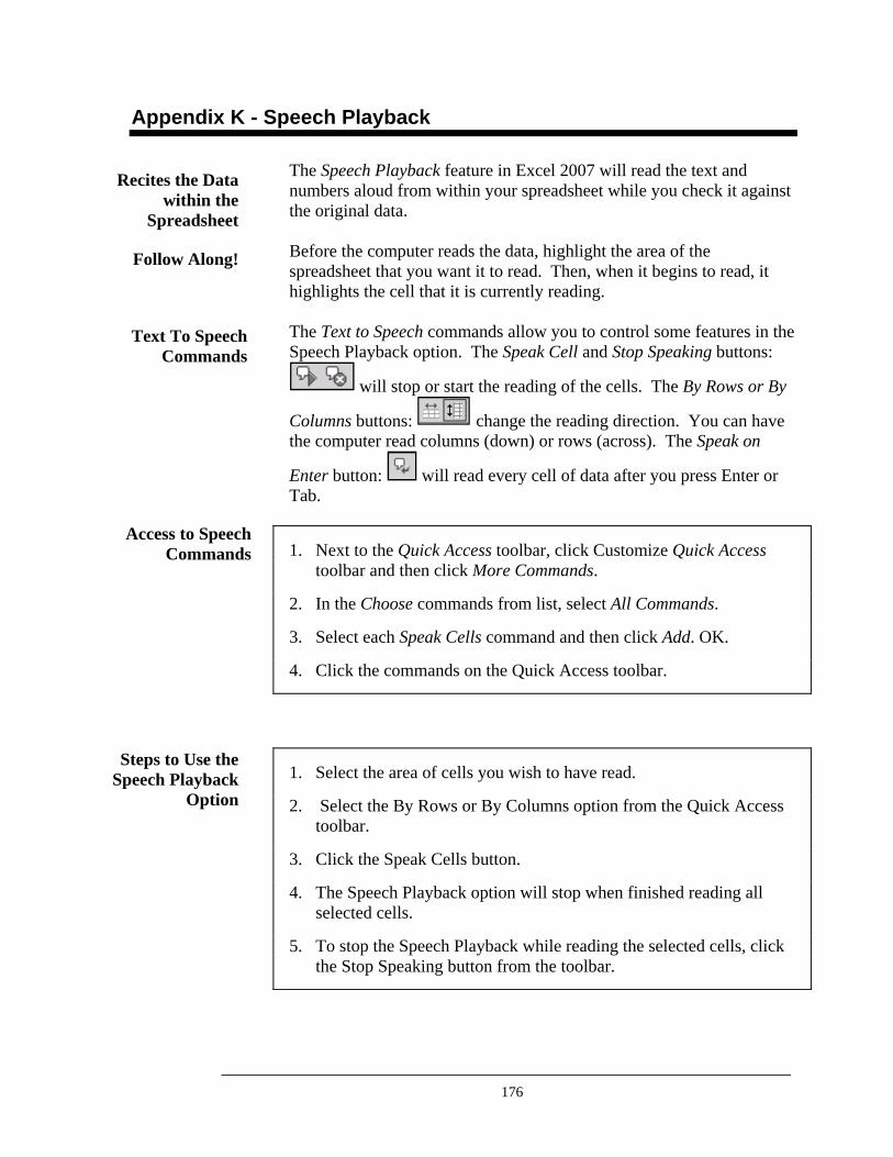
176

Appendix K - Speech Playback

The Speech Playback feature in Excel 2007 will read the text and numbers aloud from within your spreadsheet while you check it against the original data. Before the computer reads the data, highlight the area of the spreadsheet that you want it to read. Then, when it begins to read, it highlights the cell that it is currently reading. The Text to Speech commands allow you to control some features in the Speech Playback option. The Speak Cell and Stop Speaking buttons:

will stop or start the reading of the cells. The By Rows or By

Columns buttons: change the reading direction. You can have the computer read columns (down) or rows (across). The Speak on

Enter button: will read every cell of data after you press Enter or Tab.

1. Next to the Quick Access toolbar, click Customize Quick Access toolbar and then click More Commands.

2. In the Choose commands from list, select All Commands.

3. Select each Speak Cells command and then click Add. OK.

4. Click the commands on the Quick Access toolbar.

1. Select the area of cells you wish to have read.

2. Select the By Rows or By Columns option from the Quick Access toolbar.

3. Click the Speak Cells button.

4. The Speech Playback option will stop when finished reading all selected cells.

5. To stop the Speech Playback while reading the selected cells, click the Stop Speaking button from the toolbar.

Recites the Data within the

Spreadsheet

Follow Along!

Text To Speech Commands

Access to Speech Commands

Steps to Use the Speech Playback

Option

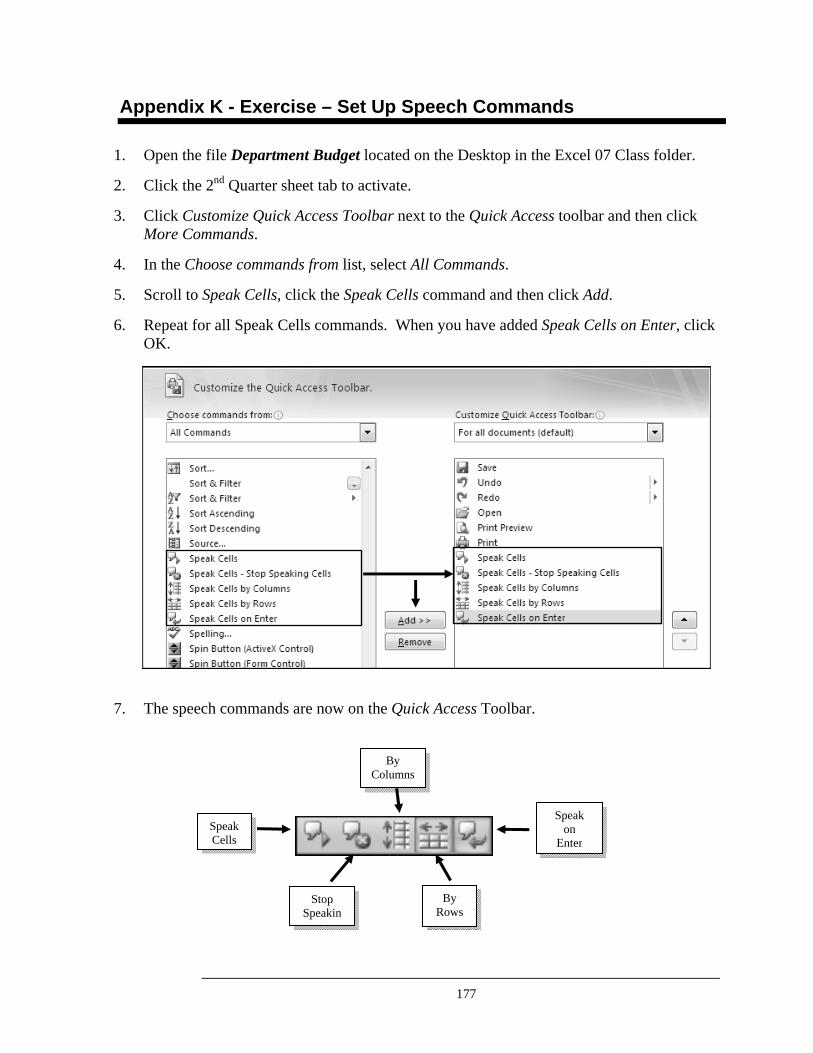
177

Appendix K - Exercise – Set Up Speech Commands

1. Open the file Department Budget located on the Desktop in the Excel 07 Class folder.

2. Click the 2nd Quarter sheet tab to activate.

3. Click Customize Quick Access Toolbar next to the Quick Access toolbar and then click More Commands.

4. In the Choose commands from list, select All Commands.

5. Scroll to Speak Cells, click the Speak Cells command and then click Add.

6. Repeat for all Speak Cells commands. When you have added Speak Cells on Enter, click OK.

7. The speech commands are now on the Quick Access Toolbar.

Stop Speakin

By Columns

Speak on

Enter Speak Cells

By Rows

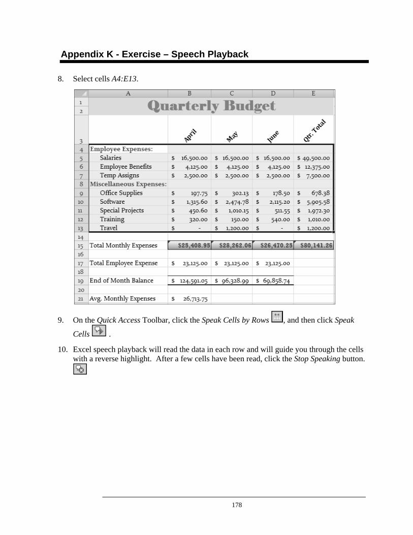
178

Appendix K - Exercise – Speech Playback

8. Select cells A4:E13.

9. On the Quick Access Toolbar, click the Speak Cells by Rows , and then click Speak

Cells .

10. Excel speech playback will read the data in each row and will guide you through the cells with a reverse highlight. After a few cells have been read, click the Stop Speaking button.

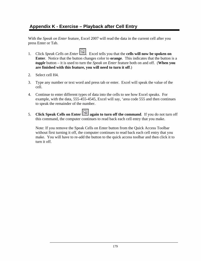
179

Appendix K - Exercise – Playback after Cell Entry

With the Speak on Enter feature, Excel 2007 will read the data in the current cell after you press Enter or Tab.

1. Click Speak Cells on Enter . Excel tells you that the cells will now be spoken on Enter. Notice that the button changes color to orange. This indicates that the button is a toggle button – it is used to turn the Speak on Enter feature both on and off. (When you are finished with this feature, you will need to turn it off.)

2. Select cell H4.

3. Type any number or text word and press tab or enter. Excel will speak the value of the cell.

4. Continue to enter different types of data into the cells to see how Excel speaks. For example, with the data, 555-455-4545, Excel will say, ‘area code 555 and then continues to speak the remainder of the number.

5. Click Speak Cells on Enter again to turn off the command. If you do not turn off this command, the computer continues to read back each cell entry that you make. Note: If you remove the Speak Cells on Enter button from the Quick Access Toolbar without first turning it off, the computer continues to read back each cell entry that you make. You will have to re-add the button to the quick access toolbar and then click it to turn it off.

180

Index

3-D Cell Reference .................................................................................. 66

Absolute Cell References ........................................................................ 64

Additional Number Formats .................................................................... 76

Appendix A – Online Help .................................................................... 162

Appendix B – Smart Tags ..................................................................... 163

Appendix C – Locking Specific Cells ................................................... 164

Appendix D – Combination Charts ....................................................... 165

Appendix E – Adding a Trendline to a Chart ........................................ 167

Appendix F – Quick Bar Charts ............................................................ 168

Appendix G – Vary Colors in the Same Data Series ............................ 169

Appendix H – Picture Charts ................................................................. 170

Appendix I – Creating Chart Templates ................................................ 172

Appendix J - Formula Names ................................................................ 174

Appendix K - Speech Playback ............................................................. 176

Borders and Colors .................................................................................. 80

Breaking the Link to the Data Source ................................................... 158

Cell Styles ................................................................................................ 82

Change Column Width & Row Height ................................................... 34

Chart Elements ...................................................................................... 135

Chart Types ........................................................................................... 136

Charts ..................................................................................................... 134

Color Code Worksheet Tabs ................................................................... 24

Combination Charts ............................................................................... 165

Comments ................................................................................................ 88

Compatibility Issues .................................................................................. 4

Conditional Formatting ......................................................................... 118

Copy & Paste a Word Table To Excel .................................................. 155

Copy Formulas (Fill Command) ............................................................. 50

Copy Formulas (Fill Handle) .................................................................. 52

Create Functions ...................................................................................... 46

181

Index

Create Tables ......................................................................................... 120

Creating Chart Templates ...................................................................... 172

Creating Charts ...................................................................................... 138

Creating Formulas ................................................................................... 42

Edit Cell Contents ................................................................................... 36

Embed a Chart into PowerPoint ............................................................ 159

Enter Numbers into Cells ........................................................................ 28

Enter Text into Cells ................................................................................ 26

Erase Cell Contents ................................................................................. 38

Exit Excel ................................................................................................ 68

Filter Data in a Table ............................................................................. 130

Formula Names ..................................................................................... 174

Formulas .................................................................................................. 40

Freeze Panes ............................................................................................ 96

Functions ................................................................................................. 44

Headers & Footers (Page Layout View) ............................................... 104

Headers and Footers (Print Preview & Page Setup) .............................. 100

Hide or Unhide Worksheets .................................................................... 20

Identify Excel 2007 Screen Components ................................................ 10

Insert and Delete Columns and Rows ..................................................... 56

Insert Functions ....................................................................................... 48

Inserting Shapes and Text Boxes ............................................................ 92

Integrating Programs – Paste & Paste Special ...................................... 154

Introduction to Excel ................................................................................. 2

Link an Excel Chart to PowerPoint Presentation .................................. 156

Locking Specific Cells .......................................................................... 164

Merge and Center .................................................................................... 58

Modify a Chart ...................................................................................... 140

Moving Within a Worksheet ................................................................... 16

Number Formats ...................................................................................... 74

182

Index

Office Button Commands Gallery ........................................................... 12

Online Help ........................................................................................... 162

Open Workbooks ..................................................................................... 70

Organization and Format Guidelines ........................................................ 3

Page Break Preview ............................................................................... 108

Page Views ............................................................................................ 106

Parts of a Formula ................................................................................... 41

Picture Charts ........................................................................................ 170

Planning a Worksheet ................................................................................ 6

Preview & Page Setup ............................................................................. 98

Print a Worksheet .................................................................................. 112

Print Embedded Chart ........................................................................... 150

Print Separate Chart Sheet ..................................................................... 152

Printing Several Worksheets ................................................................. 114

Quick Bar Charts ................................................................................... 168

Rename/Rearrange Worksheets .............................................................. 22

Save a Workbook .................................................................................... 30

Select Cells .............................................................................................. 32

Smart Tags ............................................................................................. 163

Sort Data in a Table ............................................................................... 126

Speech Playback .................................................................................... 176

Spell Check ............................................................................................ 110

Start Excel ................................................................................................. 8

Tables .................................................................................................... 120

Tables Managing Data .......................................................................... 122

Templates .............................................................................................. 172

Text Formats ............................................................................................ 72

Themes .................................................................................................... 86

Trendline ............................................................................................... 167

Updating Linked Data ........................................................................... 157

183

Index

Vary Colors in the Same Data Series .................................................... 169

View the Excel Ribbon Tabs ................................................................... 14

What- If Analysis .................................................................................. 116

Worksheet Management .......................................................................... 18

Wrap Text within a Cell .......................................................................... 78

Zoom ....................................................................................................... 60

Documents

Excel 2007 Manual. Describe the components of an Excel worksheet. 3. Move within the worksheet. 4. ... Along with the new features of Microsoft Excel 2007 come several